A Multiproduct Network Economic Model of Cybercrime

in

Financial Services

Anna Nagurney

Department of Operations and Information Management

Isenberg School of Management

University of Massachusetts

Amherst, Massachusetts 01003

September 2014; revised January 2015

Service Science (2015), 7(1), pp 70-81.

Abstract: In this paper, we propose a network economic model of cybercrime with a focus

on financial services, since such organizations are one of the principal targets of such illicit

activity. The model is a multiproduct one and constructed as a layered bipartite network

with supply price, transaction cost, and demand price functions linking the networks. A

novelty of the new model is the incorporation of average time associated with illicit product

delivery at the demand markets with the demand price functions being decreasing functions

of such times, as noted in reality. The governing equilibrium conditions are formulated as

a variational inequality problem with qualitative properties of the solution presented. An

algorithm, with nice features for computations, is then applied to two sets of numerical

examples in order to illustrate the model and computational procedure as well as the types

of interventions that can be investigated from a policy perspective to make it more difficult

for cybercriminals to obtain sensitive data.

Keywords: cybercrime, network economics, financial services, cybersecurity

1

1. Introduction

The Internet has revolutionized the way in which individuals and organizations, as well

as businesses and governments, communicate, interact, and conduct economic and social

activities. According to Internet Live Stats (2014), it is expected that there will be 3 billion

Internet users by the end of 2014 with the first billion reached only in 2005. Coupled with the

growth of the Internet as well as the multiple ways of accessing it through mobile devices, for

example, there has been a concomitant increase in cybercrime. Cybercrime is “any criminal

offense that is committed or facilitated through the use of the communication capabilities

of computers and computer systems” (Petee et al. (2010)). The Center for Strategic and

International Studies (2014) reports that the estimated annual cost to the global economy

from cybercrime is more than $400 billion with a conservative estimate being $375 billion in

losses, more than the national income of most countries.

As noted by Ablon, Libicki, and Golay (2014), the black market for cybercrime products

can be more profitable than the illegal drug trade. Links to end-users or consumers are more

direct than in the case of physical goods, and because worldwide distribution is accomplished

electronically, the requirements are negligible. A majority of the involved decision-makers,

products, and services are online-based and can be instantaneously accessed. The trans-

portation or shipment of pilfered digital goods may only require an email or download, or a

username and password to a locked site.

However, not all industries and economic sectors are affected equally by cybercrime.

According to the PriceWaterhouseCoopers 2014 Global Economic Crime Survey, 39% of

financial sector respondents said they had been victims of cybercrime, compared with only

17% in other industries, with cybercrime now the second most commonly reported economic

crime affecting financial services firms. Indeed, Wilson (2013) noted that “every minute, of

every hour, of ever day, a major financial institution is under attack.” The Ponemon Institute

(2013) determined that the average annualized cost of cybercrime for 60 organizations in

their study is $11.6 million per year, with a range of $1.3 million to $58 million. In 2012, the

average annualized cost was $8.9 million, an increase in cost of 26 percent or $2.6 million from

the results of the 2012 cyber cost study. Cyberattacks are intrusive and economically costly.

In addition, they may adversely affect a company’s most valuable asset – its reputation.

According to Sarnikar and Johnson (2009), a secure financial market system is critical

to our national economy, with statistics on incident reports collected and disseminated by

the Computer Emergency Response Team (CERT) demonstrating that a disproportionate

number of security incidents occur in the financial industry. With financial service firms

2

providing one of the critical infrastructure networks on which our economy and society

depends, it is imperative to be able to assess their vulnerabilities to cyberattacks in a rigorous,

quantifiable manner as well as to identify possible synergies associated with information

sharing. Only by capturing the complexities and the underlying behavior can one then

mitigate the risk as well as identify where to invest in order to secure the financial networks

on which so many of the financial transactions now depend.

In this paper, we lay the foundation for the development of network economics based

models for cybercrime in financial services. We use, as the basis, spatial network economic

models, presenting a new multiproduct one, in which we incorporate the critical time compo-

nent associated with transactions. For example, it is recognized (cf. Leinwand Leger (2014))

that there is a short time window during which the value of a financial product acquired

through cybercrime is positive but it decreases during the time window. As reported therein,

following the major Target breach, credit cards obtained thus initially sold for $120 each on

the black market, but, within weeks, as banks started to cancel the cards, the price dropped

to $8 and, seven months after Target learned about the breach, the cards had essentially

no value. In addition, different “brands” of credit cards can be viewed as different products

since they command different prices on the black market. For example, according to Lein-

wand Leger (2014) credit cards with the highest credit limits, such as an American Express

Platinum card, command the highest prices. A card number with a low limit might sell for

$1 or $2, while a high limit card number can sell for $15 or considerably more, as noted

above. Hacked credit card numbers of European credit cards can command prices five times

higher than U.S. cards (see Peterson (2013)). For some background on the economics of

stolen credentials and the methods used to monetize them, see Shulman (2010). Moreover,

according to Mandiant (2014), in 2013, the median number of days cyberattackers were

present on a victim network before they were discovered was 229 days, pointing to again the

critical time element associated with cybercrime and associated costs.

Our view is that financial firms produce/possess products that hackers (criminals) seek

to obtain. Both financial services firms as well as hackers are economic agents. We assume

that the firms (as well as the hackers) can be located in different regions of a country or

in different countries (cf. Perlroth and Gelles (2014)). Financial service firms may also

be interpreted as prey and the hackers as predators. Products that the criminals seek

to acquire may include: credit card numbers, email addresses and password information,

personal credentials, specific documents, etc. The financial firms are the producers of these

products whereas the hackers act as agents and “sell” these products, if they acquire them,

at the “going” market prices. There is a “price” at which the hackers acquire the financial

3

product and a price at which they sell the hacked product in the demand markets. The

former we refer to as the supply price and the latter is the demand price. In addition, we

assume that there is a transaction cost associated between each pair of financial and demand

markets for each product. These transaction costs can be generalized costs that also capture

risk associated with being “caught.” Associated with the product demand price functions is

also a time.

By constructing an appropriate computational network economic framework as a foun-

dation, numerous scenarios can then be investigated, as well as policies evaluated. Indeed,

Ablon, Liwicki, and Golay (2014) have argued in their study that an economic approach to

tackling cybercrime in warranted.

In the financial network cybercrime problem, we seek to determine the supply prices, the

demand prices, and the hacked product trade flows satisfying the equilibrium condition that,

for each financial product, the demand price is equal to the supply price plus the transaction

cost, if there is “trade” between the pair of financial and demand markets; if the demand

price is less than the supply price plus the transaction cost, then there will be no (illicit)

trade. Indeed, if the cybercriminals do not find demand markets for their acquired financial

products (since there are no consumers willing to pay the price) then there is no economic

incentive for them to acquire the financial products. To present another criminal network

analogue – consider the market for illegal drugs, with the U.S. market being one of the

largest, if not the largest one. If there is no demand for the drugs then the suppliers of

illegal drugs cannot recover their costs of production and transaction and the flows of drugs

will go to zero.

Since the framework that we utilize as the foundation for our modeling, analysis, and,

ultimately, policy-making recommendations is that of spatial economics and network equi-

librium, we now, for completeness, provide some of the historical background with the sup-

porting literature. Further background can be found in the books by Nagurney (1999, 2003,

2006) with analogues to financial networks made in the book by Nagurney and Siokos (1997).

Enke (1951) established the connection between spatial price equilibrium problems and

electronic circuit networks and showed that this analogue could then be used to compute

the spatial prices and commodity flows. Subsequently, the Nobel laureate Samuelson (1952)

and Takayama and Judge (1964, 1971) showed that the prices and commodity flows satis-

fying the spatial price equilibrium conditions could be determined, under certain symmetry

assumptions, by solving an extremal problem, in other words, a mathematical programming

problem. This theoretical advance enabled not only the qualitative study of equilibrium

4

patterns, but also opened up the possibility for the development of effective computational

procedures. Moreover, it unveiled a wealth of potential applications. Subsequent advances in

methodologies, such as variational inequality theory, have allowed for the modeling of price

and cost asymmetries as well as multiple commodities (see, e.g., Nagurney (1999)). Thus

far, spatial price equilibrium models have been used to study problems in agriculture, energy

markets, and mineral economics, as well as in finance (see, e.g., Judge and Takayama (1973)

and Nagurney (1992, 1999), and the references therein) and, more recently, in predator prey

ecological networks (cf. Nagurney and Nagurney (2012)).

The methodology that we utilize for the formulation, analysis, and computations is vari-

ational inequality theory. Altough the models that we construct are perfectly competitive

ones they are linked to game theoretic formalisms (see, e.g., Dafermos and Nagurney (1987))

and Nash equilibria. A recent survey of game theory and network security is given by Man-

shaei et al. (2011). Our perfectly competitive network economic framework utilizes time

concepts from time-based competition in supply chain networks in imperfectly competitive,

that is, oligopolistic supply chain markets (see Nagurney and Yu (2014) and Nagurney et al.

(2013, 2014)). Specifically, as discussed earlier, we have the value of the financial product

decrease in time as reflected through the price.

The paper is organized as follow. In Section 2 we present the model, along with its

qualitative properties. In Section 3 we outline the computational procedure, along with

convergence results, which we then utilize in Section 4 to compute solutions to a spectrum

of numerical examples. We summarize our results and present our conclusions in Section 5.

5

m m m

m m m

1 2 · · · n

1 2 · · · m

Demand Markets

Source Locations

?

AAAAAAAAU

QQ

QQ

QQ

QQ

QQ

Qs

��

��

��

��� ?

@@

@@

@@

@@R?

��

��

��

��

��

��

��

��

��

�+

Financial Product 1

m m m

m m m

1 2 · · · n

1 2 · · · m

Source Locations

Demand Markets

?

AAAAAAAAU

QQ

QQ

QQ

QQ

QQ

Qs

��

��

��

��� ?

@@

@@

@@

@@R?

��

��

��

��

��

��

��

��

��

�+

Financial Product o

··

··

··

·

··

··

··

·

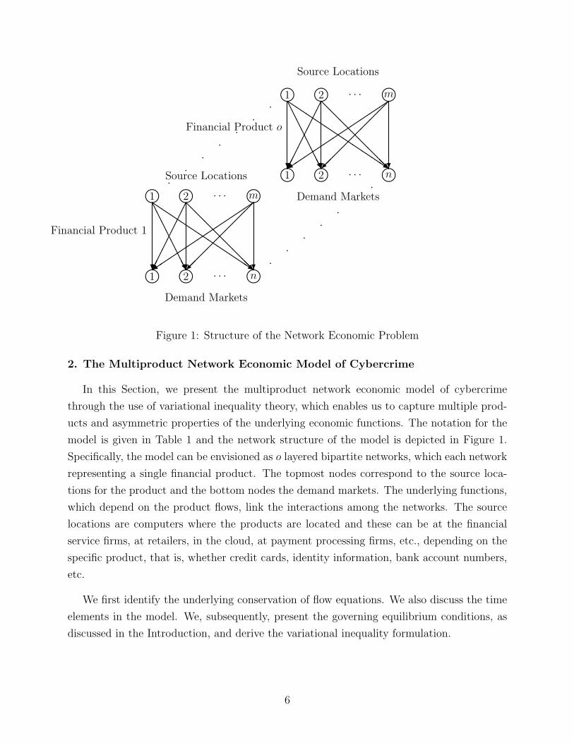
Figure 1: Structure of the Network Economic Problem

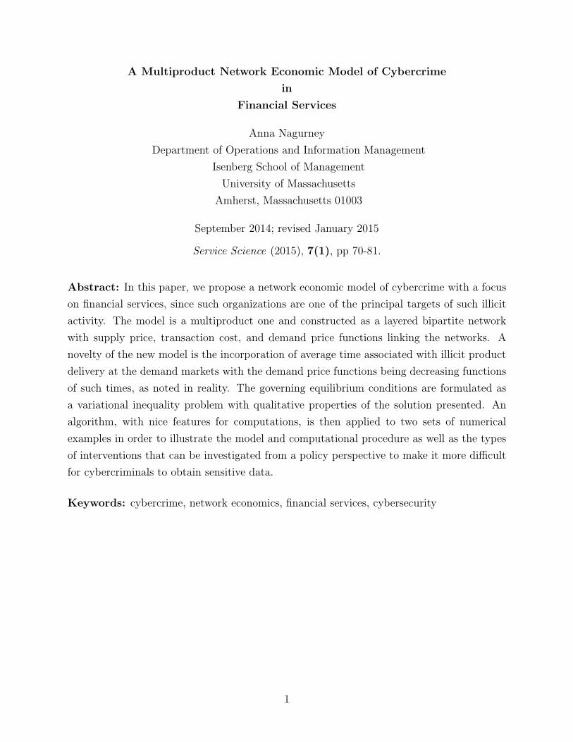
2. The Multiproduct Network Economic Model of Cybercrime

In this Section, we present the multiproduct network economic model of cybercrime

through the use of variational inequality theory, which enables us to capture multiple prod-

ucts and asymmetric properties of the underlying economic functions. The notation for the

model is given in Table 1 and the network structure of the model is depicted in Figure 1.

Specifically, the model can be envisioned as o layered bipartite networks, which each network

representing a single financial product. The topmost nodes correspond to the source loca-

tions for the product and the bottom nodes the demand markets. The underlying functions,

which depend on the product flows, link the interactions among the networks. The source

locations are computers where the products are located and these can be at the financial

service firms, at retailers, in the cloud, at payment processing firms, etc., depending on the

specific product, that is, whether credit cards, identity information, bank account numbers,

etc.

We first identify the underlying conservation of flow equations. We also discuss the time

elements in the model. We, subsequently, present the governing equilibrium conditions, as

discussed in the Introduction, and derive the variational inequality formulation.

6

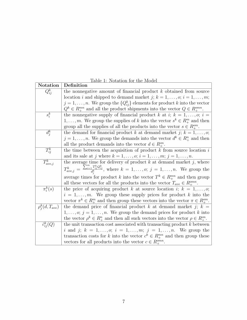
Table 1: Notation for the ModelNotation Definition

Qkij the nonnegative amount of financial product k obtained from source

location i and shipped to demand market j; k = 1, . . . , o; i = 1, . . . ,m;j = 1, . . . , n. We group the {Qk

ij} elements for product k into the vectorQk ∈ Rmn

+ and all the product shipments into the vector Q ∈ Romn+ .

ski the nonnegative supply of financial product k at i; k = 1, . . . , o; i =

1, . . . ,m. We group the supplies of k into the vector sk ∈ Rm+ and then

group all the supplies of all the products into the vector s ∈ Rom+ .

dkj the demand for financial product k at demand market j; k = 1, . . . , o;

j = 1, . . . , n. We group the demands into the vector dk ∈ Rn+ and then

all the product demands into the vector d ∈ Ron+ .

T kij the time between the acquisition of product k from source location i

and its sale at j where k = 1, . . . , o; i = 1, . . . ,m; j = 1, . . . , n.T k

ave,j the average time for delivery of product k at demand market j, where

T kave,j =

∑m

i=1T k

ijQkij

dkj

, where k = 1, . . . , o; j = 1, . . . , n. We group the

average times for product k into the vector T k ∈ Rmn+ and then group

all these vectors for all the products into the vector Tave ∈ Romn+ .

πki (s) the price of acquiring product k at source location i; k = 1, . . . , o;

i = 1, . . . ,m. We group these supply prices for product k into thevector πk ∈ Rm

+ and then group these vectors into the vector π ∈ Rom+ .

ρkj (d, Tave) the demand price of financial product k at demand market j; k =

1, . . . , o; j = 1, . . . , n. We group the demand prices for product k intothe vector ρk ∈ Rn

+ and then all such vectors into the vector ρ ∈ Ron+ .

ckij(Q) the unit transaction cost associated with transacting product k between

i and j; k = 1, . . . , o; i = 1, . . . ,m; j = 1, . . . , n. We group thetransaction costs for k into the vector ck ∈ Rmn

+ and then group thesevectors for all products into the vector c ∈ Romn

+ .

7

The conservation of flow equations are:

ski =

n∑j=1

Qkij, k = 1, . . . , o; i = 1, . . . ,m, (1)

dkj =

m∑i=1

Qkij, k = 1, . . . , o; i = 1, . . . , n, (2)

Qkij ≥ 0, k = 1, . . . , o; i = 1, . . . ,m; j = 1, . . . , n. (3)

According to (1), for each financial product, the supply (amount pilfered) at a location is

equal to the sum of the flows of the product to all the demand markets. Similarly, according

to (2), the (illicit) demand for a financial product at each demand market is equal to the

sum of the flows of that product from all source locations to the demand market. Finally,

(3) formalizes that the financial product flows are nonnegative.

In addition, we introduce the following expression, which captures time:

tkijQkij + hk

ij = T kij, k = 1, . . . , o; i = 1, . . . ,m; j = 1, . . . , n, (4)

where the hkij terms are positive and the tkij terms are nonnegative. The time expressions in

(4) capture the delay associated with the cybercrime activity and the sale of the product on

the black market. This time also, in a sense, can reflect the time associated with the financial

service firms learning about the breach. As noted in the Introduction, the value or price of

the financial product depends not only on the quantity on the black market but also the

time. Indeed according to Brian Krebs (cf. Leinwand Leger (2014)) “The most important

part of the price is the freshness, before the victim knows they’ve been breached and when

no one is canceling.” “The guarantees on the cards dwindle the older they get.” Hence,

certain financial products that are targets of cybercriminals actually have a perishability

characteristic which can be viewed as a deterioration in quality in the context of supply

chain networks (cf. Nagurney et al. (2014)).

As can be seen from Table 1, the demand price functions depend on the vector of financial

products and also on the vector (in general) of the average delivery times of the pilfered

financial products at the demand markets. Average time concepts have been used in the

context of supply chain networks with demand price functions being decreasing functions

of average times (cf. Nagurney et al. (2014)). In view of (4) and (3), we can define new

demand price functions ρkj , ∀k,∀j (cf. Table 1) as follows:

ρkj (Q) ≡ ρk

j (d, Tave), k = 1, . . . , o; j = 1, . . . , n. (5)

8

If the demand at a demand market for a product is equal to zero, we remove that demand

market from the network for that product since the corresponding time average would not

be defined.

Also, in view of (1) we can define new supply price functions πki , ∀k,∀i (cf. Table 1) as:

πki (Q) ≡ πk

i (s), k = 1, . . . , o; j = 1, . . . , n, (6)

which allow us to construct a variational inequality formulation governing the equilibrium

conditions below with nice features for computations. We assume that all the functions in

the model are continuous.

2.1 The Network Economic Equilibrium Conditions

The network economic equilibrium conditions for cybercrime have been achieved if for all

products k; k = 1, . . . , o, and for all pairs of markets (i, j); i = 1, . . . ,m; j = 1, . . . , n, the

following conditions hold:

πki (Q∗) + ck

ij(Q∗)

{= ρk

j (Q∗), if Qk

ij∗

> 0≥ ρk

j (Q∗), if Qk

ij∗

= 0,(7)

where recall that πki denotes the price of product k at source location i, ck

ij denotes the unit

transaction cost associated with k between (i, j), and ρkj is the demand price of k at demand

market j. Qkij∗

is the equilibrium flow of product k between i and j with Q∗ being the vector

of all such flows.

The equilibrium conditions (7) reflect that cybercriminals will have no incentive to acquire

a financial product at a location if the price associated with acquiring it plus the unit

transaction cost exceeds the price that they are able to get for the product at the demand

(black) market. They will acquire the product at a source location and will trade it if the

demand price for the product at the demand market is equal to the acquiring (or supply)

price plus the unit transaction cost. These are the well-known spatial price equilibrium

conditions (cf. Samuelson (1952), Takayama and Judge (1971), Florian and Los (1982),

Dafermos and Nagurney (1984), Thore (1991), Nagurney (1999) and the references therein)

adapted to the illicit cybercrime application but with the novelty of embedded times in the

demand price functions.

We define the feasible set K ≡ {Q|Q ∈ Romn+ }.

9

Theorem 1: Variatinal Inequality Formulation

A product flow pattern Q∗ ∈ K is a cybercrime network economic equilibrium if and only if

it satisfies the variational inequality problem:

o∑k=1

m∑i=1

n∑j=1

[πk

i (Q∗) + ckij(Q

∗)− ρkj (Q

∗)]× (Qk

ij −Qkij

∗) ≥ 0, ∀Q ∈ K. (8)

Proof: We first establish necessity, that is, if Q∗ ∈ K satisfies the network economic equi-

librium conditions for cybercrime given by (7) then it also satisfies variational inequality

(8).

From (7), we have that, for a fixed k and (i, j) pair:[πk

i (Q∗) + ckij(Q

∗)− ρkj (Q

∗)]×

[Qk

ij −Qkij

∗] ≥ 0, ∀Qkij ≥ 0. (9)

.

Indeed, if Qkij∗

> 0, then, according to (7), the term before the multiplication sign in (9) is

equal to zero, so the inequality holds true and, if Qkij∗

= 0, then both terms on the left-hand

side of the ≥ 0 expression in (9) are nonnegative so their product is also nonnegative.

But (9) holds for each product k and every pair (i, j); hence, summation of (9) over all

k, i, j yields:

o∑k=1

m∑i=1

n∑j=1

[πk

i (Q∗) + ckij(Q

∗)− ρkj (Q

∗)]×

[Qk

ij −Qkij

∗] ≥ 0, ∀Qkij ≥ 0,∀k, i, j, (10)

which is precisely variational inequality (8)

We now establish sufficiency, that is, a solution to variational inequality (8) also satisfies

the economic equilibrium conditions (7).

Into (8), we make the following substitution. We set: Qkij = Qk

ij∗

for all k 6= l; i 6= p;

j 6= q. (8) then collapses to:[πl

pq(Q∗) + cl

pq(Q∗)− ρl

q(Q∗)

]×

[Ql

pq −Qlpq

∗] ≥ 0, ∀Qlpq ≥ 0. (11)

From (11) we see that, if Qlpq∗

> 0, then since[Ql

pq −Qlpq∗]

may be positive, negative, or

zero, this implies that: [πl

pq(Q∗) + clpq(Q

∗)− ρlq(Q

∗)]

= 0, (12)

10

which is the first part of the cybercrime network economic equilibrium conditions (7).

On the other hand, if Qlpq∗

= 0, then we know that[πl

pq(Q∗) + cl

pq(Q∗)− ρl

q(Q∗)

]≥ 0, (13)

since Qlpq ≥ 0 by assumption of nonnegative product flows, and (13) is simply the second

part of the economic equilibrium conditions (7).

The above arguments hold for any financial product and pair of markets; hence, we have

established sufficiency. 2

We now put variational inequality problem (8) into standard form (see Nagurney (1999)):

determine X∗ ∈ K, such that

〈F (X∗), X −X∗〉 ≥ 0, ∀X ∈ K. (14)

Specifically, we define K ≡ K, X ≡ Q, and F (X) ≡ (Fkij(X)); k = 1, . . . , o; i = 1, . . . ,m;

j = 1, . . . , n, where Fkij = πki (Q) + ck

ij(Q)− ρkj (Q).

In order to compute solutions to the above described financial service firm network eco-

nomic cybersecurity models, one can avail oneself of numerous algorithms that exploit the

special network structure. For details, see Nagurney and Aronson (1988, 1989), Nagurney

and Kim (1989), Nagurney (1987, 1989, 1999, 2006) and the references therein. Before

proposing an algorithm that we will use to compute solutions to the numerical examples, we

first provide some qualitative properties of the equilibrium pattern.

2.2 Qualitative Properties

Since the feasible setK in our model is not compact, that is. closed and bounded, existence

of a solution is not guaranteed unless other conditions are satisfied from the standard theory

of variationa inequalities (see Kinderlehrer and Stampacchia (1980) and Nagurney (1999)).

We could, of course, assume that both the demands and the supplies of the financial products

are finite (although they may be very large), and, hence, the product flows will also be

bounded. If this is the case then a solution to variational inequality (8) is guaranteed since

the function F (X) that enters the equivalent variational inequality (14) is continuous under

the assumptions made earlier that the underlying functions (supply price, demand price, and

unit transaction costs) are continuous. It would then follow that there would be a unique

solution to (14) (and (8)) if the function F (X) in our model was strictly monotone, that is:

〈F (X1)− F (X2), X1 −X2〉 > 0, ∀X1, X2 ∈ K, X1 6= X2. (15)

11

Under the slightly stronger condition of strong monotonicity, that is, if

〈F (X1)− F (X2), X1 −X2〉 ≥ 0, ∀X1, X2 ∈ K, (16)

we are guaranteed both existence and uniqueness of a solution X∗ to (14).

Moreover, we know (cf. Nagurney (1999)) that if ∇F (X) is positive-definite over K then

F (X) is strongly monotone.

3. The Algorithm

For the solution of the numerical examples in the next section, we apply the Euler method,

which is an algorithm induced by the general itartve scheme of Dupuis and Nagurney (1993).

It general statement is as follows.

The Euler Method

At each iteration τ one solves the following problem:

Xτ+1 = PK(Xτ − aτF (Xτ )), (17)

where PK is the projection operator.

As shown in Dupuis and Nagurney (1993) and Nagurney and Zhang (1996), for con-

vergence of the general iterative scheme, which induces the Euler method, among other

methods, the sequence {aτ} must satisfy:∑∞

τ=0 aτ = ∞, aτ > 0, aτ → 0, as τ →∞. Specific

conditions for convergence of this scheme can be found for a variety of network-based prob-

lems, similar to those constructed in Nagurney and Zhang (1996) and the references therein;

see also Nagurney et al. (2013), Toyasaki, Daniele, and Wakolbinger (2014), and Saberi,

Nagurney, and Wolf (2014).

The realization of (17) takes on the following explicit formulae for our model.

Explicit Formulae for (17)

In particular, we have the following closed form expression for the product flows k = 1, . . . ,m;

i = 1, . . . ,m; j = 1, . . . , n:

Qkij

τ+1= max{0, Qk

ij

τ+ aτ (ρ

kj (Q

τ )− ckij(Q

τ )− πki (Qτ )}. (18)

12

Theorem 2: Convergence

In the cybercrime network economic model, assume that F (X)) is strongly monotone and

uniformly Lipschitz continuous. Then, there exists a unique equilibrium product flow pattern

Q∗ ∈ K and any sequence generated by the Euler method as given by (17), where {aτ}satisfies

∑∞τ=0 aτ = ∞, aτ > 0, aτ → 0, as τ →∞ converges to Q∗.

Proof of the above Theorem follows from Theorem 6.10 in Nagurney and Zhang (1996).

4. Numerical Examples

The Euler method was implemented in FORTRAN and run on a Linux system at the

University of Massachusetts Amherst. The algorithm was initialized with all financial prod-

uct flows equal to 1.0. The convergence criterion ε was set to 10−4, that is, the Euler method

was deemed to have converged if the absolute value of each of the successive product flows

was less than or equal to ε.

We solved two sets of examples, each with three examples. Below we describe the exam-

ples and the results obtained.

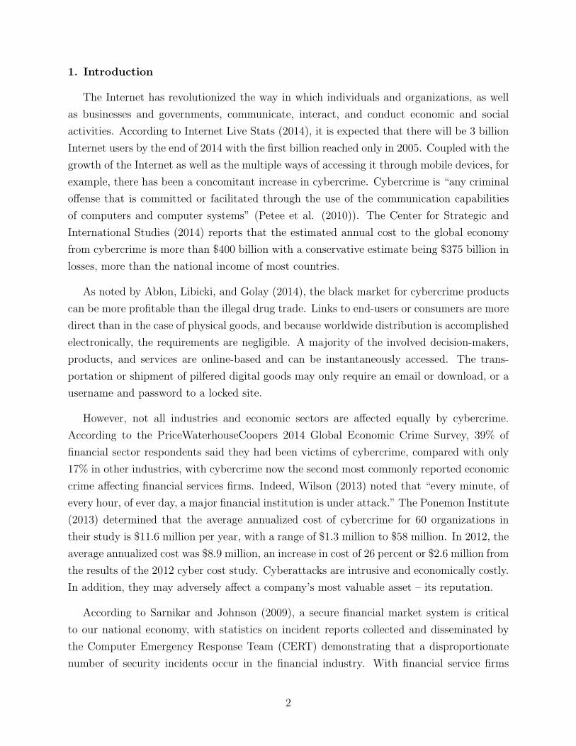
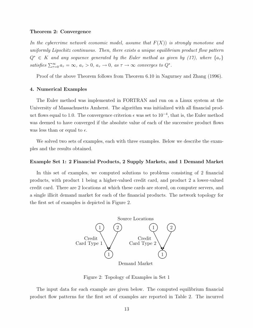
Example Set 1: 2 Financial Products, 2 Supply Markets, and 1 Demand Market

In this set of examples, we computed solutions to problems consisting of 2 financial

products, with product 1 being a higher-valued credit card, and product 2 a lower-valued

credit card. There are 2 locations at which these cards are stored, on computer servers, and

a single illicit demand market for each of the financial products. The network topology for

the first set of examples is depicted in Figure 2.

Demand Market

����1

AAAAAU

��

����

1���� ����2

CreditCard Type 1

����1

AAAAAU

��

����

1���� ����2

CreditCard Type 2

Source Locations

Figure 2: Topology of Examples in Set 1

The input data for each example are given below. The computed equilibrium financial

product flow patterns for the first set of examples are reported in Table 2. The incurred

13

equilibrium supply prices, unit transaction costs, demand prices, and average times, in turn,

are reported in Table 3.

Example 1

The data for Example 1 are below. The supply price functions are:

π11(s) = 5s1

1 + s12 + 2, π1

2(s) = 2s12 + s1

1 + 1,

π21(s) = 2s2

1 + s11 + 1, π2

2(s) = s22 + .5s1

2 + 1.

The unit transaction cost functions are:

c11(Q) = .03Q1

112+ 3Q1

11 + 1, c121(Q) = .02Q1

212+ 2Q1

21 + 2,

c211(Q) = .01Q2

112+ Q2

11 + 1, c121(Q) = .001Q2

212+ .1Q2

21 + 1,

and the demand price functions are:

ρ1(1) = −2d11 − d2

1 − .5T 1ave,1 + 500, ρ2

1(d) = −3d21 − d1

1 − .1T 2ave,1 + 300.

The time expressions are:

T 111 = .1Q1

11 + 10, T 121 = .5Q1

21 + 5,

T 211 = .1Q2

11 + 20, T 221 = .5Q2

21 + 15,

so that

T 1ave,1 =

T 111Q

111 + T 1

21Q121

d11

, T 2ave,1 =

T 211Q

211 + T 2

21Q221

d21

.

The Euler method converged to the solution reported in Tables 2 and 3 in 540 iterations.

Example 2

Example 2 was constructed from Example 1, except for the following changes. The fixed

terms in the link time functions were increased so that they are now:

T 111 = .1Q1

11 + 100, T 121 = .5Q1

21 + 50,

T 211 = .1Q2

11 + 200, T 221 = .5Q2

21 + 150.

This kind of change could reflect that it is becoming more difficult for the cybercriminals to

fence the pilfered credit card information. As a consequence, the prices drop for both financial

products at the demand market, and the average time for delivery increases substantially.

The Euler method required 539 iterations for convergence.

14

Example 3

Example 3, in turn, was constructed from Example 2 with the data identical to that in

Example 2 except for new supply price functions, which are now:

π11(s) = 5s1

1 + s12 + 200, π1

2(s) = 2s12 + s1

1 + 200,

π21(s) = 2s2

1 + s11 + 100, π2

2(s) = s22 + .5s1

2 + 100.

In particular, the fixed term components were increased substantially to investigate the

impact, from a policy or investment perspective, of making it more difficult to attack the

computer servers and have the financial information extracted from them. There is now

a slight decrease in the average times, as compared to the results for Example 2 and a

significant increase in the demand market prices for the two products.

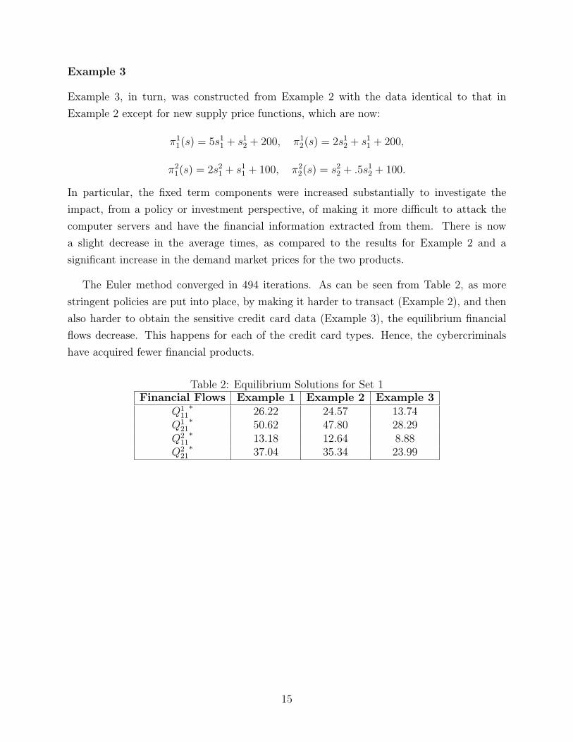
The Euler method converged in 494 iterations. As can be seen from Table 2, as more

stringent policies are put into place, by making it harder to transact (Example 2), and then

also harder to obtain the sensitive credit card data (Example 3), the equilibrium financial

flows decrease. This happens for each of the credit card types. Hence, the cybercriminals

have acquired fewer financial products.

Table 2: Equilibrium Solutions for Set 1Financial Flows Example 1 Example 2 Example 3

Q111∗

26.22 24.57 13.74Q1

21∗

50.62 47.80 28.29Q2

11∗

13.18 12.64 8.88Q2

21∗

37.04 35.34 23.99

15

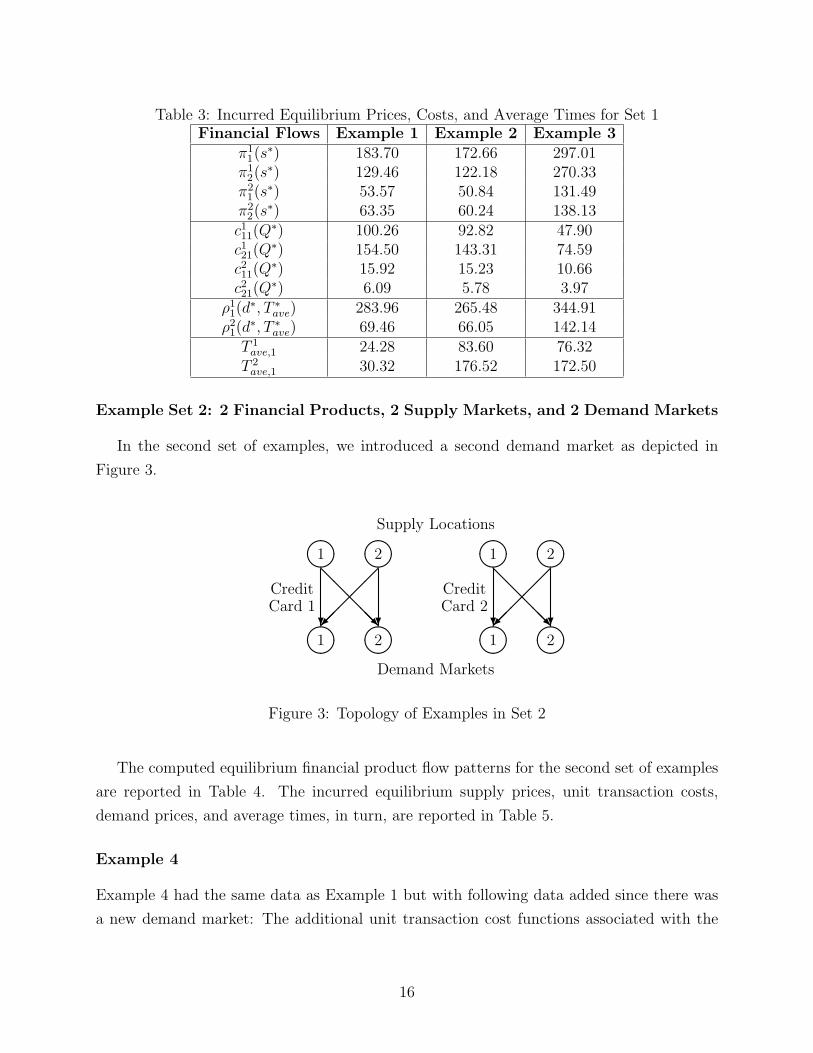
Table 3: Incurred Equilibrium Prices, Costs, and Average Times for Set 1Financial Flows Example 1 Example 2 Example 3

π11(s

∗) 183.70 172.66 297.01π1

2(s∗) 129.46 122.18 270.33

π21(s

∗) 53.57 50.84 131.49π2

2(s∗) 63.35 60.24 138.13

c111(Q

∗) 100.26 92.82 47.90c121(Q

∗) 154.50 143.31 74.59c211(Q

∗) 15.92 15.23 10.66c221(Q

∗) 6.09 5.78 3.97ρ1

1(d∗, T ∗ave) 283.96 265.48 344.91

ρ21(d

∗, T ∗ave) 69.46 66.05 142.14T 1

ave,1 24.28 83.60 76.32T 2

ave,1 30.32 176.52 172.50

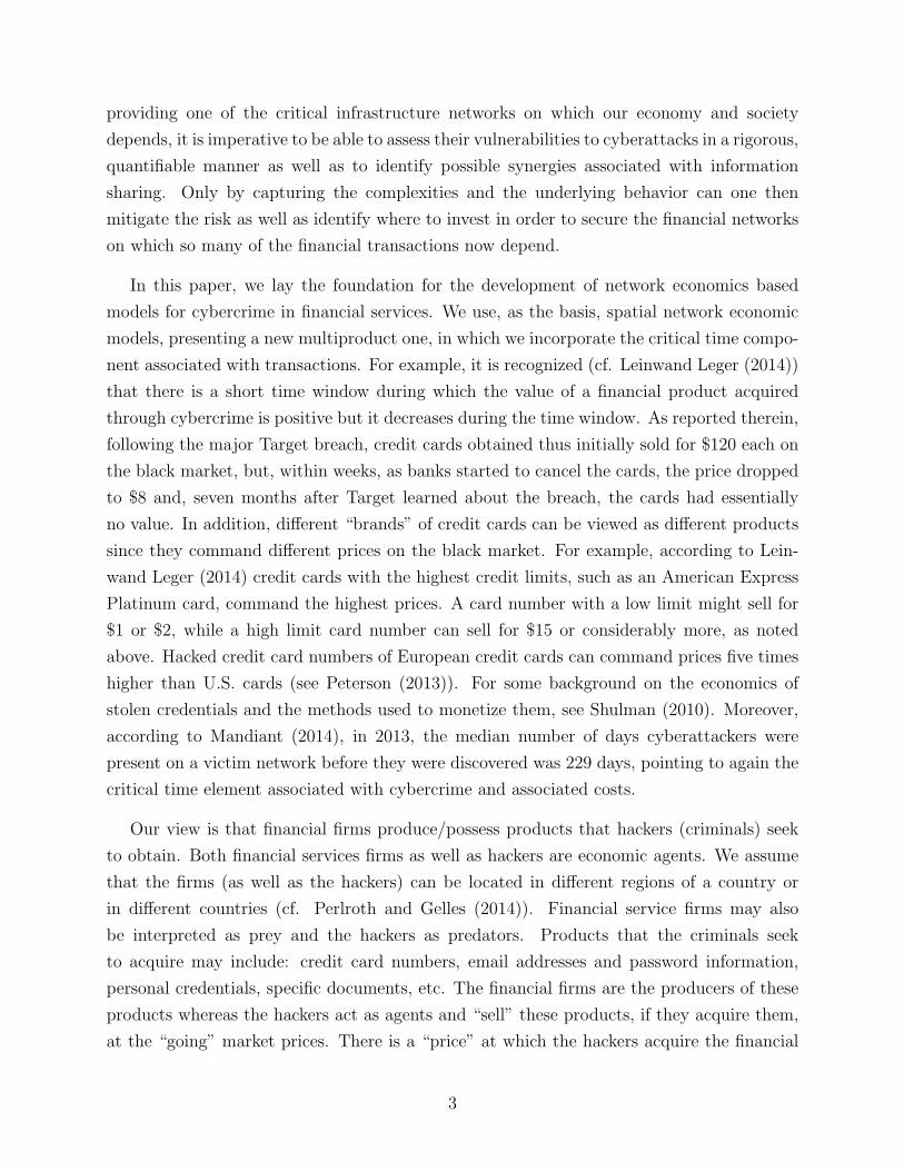
Example Set 2: 2 Financial Products, 2 Supply Markets, and 2 Demand Markets

In the second set of examples, we introduced a second demand market as depicted in

Figure 3.

Demand Markets

����1 ����

2?

@@

@@@R?

��

���

1���� ����2

CreditCard 1

����1 ����

2?

@@

@@@R?

��

���

1���� ����2

CreditCard 2

Supply Locations

Figure 3: Topology of Examples in Set 2

The computed equilibrium financial product flow patterns for the second set of examples

are reported in Table 4. The incurred equilibrium supply prices, unit transaction costs,

demand prices, and average times, in turn, are reported in Table 5.

Example 4

Example 4 had the same data as Example 1 but with following data added since there was

a new demand market: The additional unit transaction cost functions associated with the

16

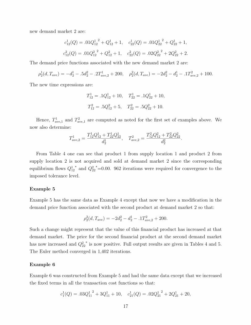
new demand market 2 are:

c112(Q) = .01Q1

122+ Q1

12 + 1, c122(Q) = .01Q1

222+ Q1

22 + 1,

c212(Q) = .01Q2

122+ Q2

12 + 1, c222(Q) = .02Q2

222+ 2Q2

22 + 2.

The demand price functions associated with the new demand market 2 are:

ρ12(d, Tave) = −d1

2 − .5d22 − .2T 1

ave,2 + 200, ρ22(d, Tave) = −2d2

2 − d12 − .1T 2

ave,2 + 100.

The new time expressions are:

T 112 = .1Q1

12 + 10, T 122 = .1Q1

22 + 10,

T 212 = .5Q2

12 + 5, T 222 = .5Q2

22 + 10.

Hence, T 1ave,1 and T 2

ave,1 are computed as noted for the first set of examples above. We

now also determine:

T 1ave,2 =

T 112Q

112 + T 1

22Q122

d12

, T 2ave,2 =

T 212Q

212 + T 2

22Q222

d22

.

From Table 4 one can see that product 1 from supply location 1 and product 2 from

supply location 2 is not acquired and sold at demand market 2 since the corresponding

equilibrium flows Q112∗

and Q222∗=0.00. 962 iterations were required for convergence to the

imposed tolerance level.

Example 5

Example 5 has the same data as Example 4 except that now we have a modification in the

demand price function associated with the second product at demand market 2 so that:

ρ22(d, Tave) = −2d2

2 − d12 − .1T 2

ave,2 + 200.

Such a change might represent that the value of this financial product has increased at that

demand market. The price for the second financial product at the second demand market

has now increased and Q222∗

is now positive. Full output results are given in Tables 4 and 5.

The Euler method converged in 1,402 iterations.

Example 6

Example 6 was constructed from Example 5 and had the same data except that we increased

the fixed terms in all the transaction cost functions so that:

c11(Q) = .03Q1

112+ 3Q1

11 + 10, c121(Q) = .02Q1

212+ 2Q1

21 + 20,

17

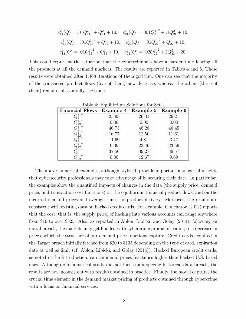
c211(Q) = .01Q2

112+ Q2

11 + 10, c121(Q) = .001Q2

212+ .1Q2

21 + 10,

c112(Q) = .01Q1

122+ Q1

12 + 10, c122(Q) = .01Q1

222+ Q1

22 + 10,

c212(Q) = .01Q2

122+ Q2

12 + 10, c222(Q) = .02Q2

222+ 2Q2

22 + 20.

This could represent the situation that the cybercriminals have a harder time fencing all

the products at all the demand markets. The results are reported in Tables 4 and 5. These

results were obtained after 1,468 iterations of the algorithm. One can see that the majority

of the transacted product flows (five of them) now decrease, whereas the others (three of

them) remain substantially the same.

Table 4: Equilibrium Solutions for Set 2Financial Flows Example 4 Example 5 Example 6

Q111∗

25.93 26.31 26.21Q1

12∗

0.00 0.00 0.00Q1

21∗

46.73 48.28 46.45Q1

22∗

16.77 12.50 11.61Q2

11∗

11.69 4.81 3.47Q2

12∗

6.09 23.46 23.59Q2

21∗

37.56 39.27 39.57Q2

22∗

0.00 12.67 9.69

The above numerical examples, although stylized, provide important managerial insights

that cybersecurity professionals may take advantage of in securing their data. In particular,

the examples show the quantified impacts of changes in the data (the supply price, demand

price, and transaction cost functions) on the equilibrium financial product flows, and on the

incurred demand prices and average times for product delivery. Moreover, the results are

consistent with existing data on hacked credit cards. For example, Goncharov (2012) reports

that the cost, that is, the supply price, of hacking into various accounts can range anywhere

from $16 to over $325. Also, as reported in Ablon, Libicki, and Golay (2014), following an

initial breach, the markets may get flooded with cybercrime products leading to a decrease in

prices, which the structure of our demand price functions capture. Credit cards acquired in

the Target breach initially fetched from $20 to $135 depending on the type of card, expiration

date as well as limit (cf. Ablon, Libicki, and Golay (2014)). Hacked European credit cards,

as noted in the Introduction, can command prices five times higher than hacked U.S. based

ones. Although our numerical study did not focus on a specific historical data breach, the

results are not inconsistent with results obtained in practice. Finally, the model captures the

crucial time element in the demand market pricing of products obtained through cybercrime

with a focus on financial services.

18

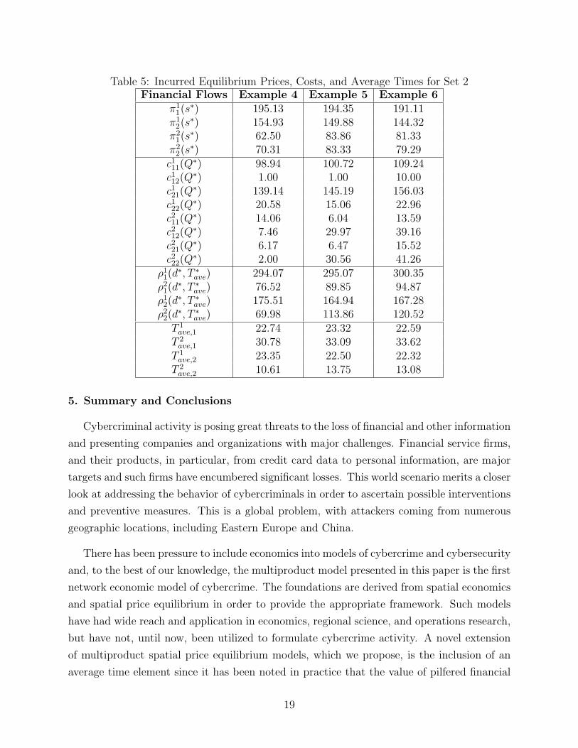
Table 5: Incurred Equilibrium Prices, Costs, and Average Times for Set 2Financial Flows Example 4 Example 5 Example 6

π11(s

∗) 195.13 194.35 191.11π1

2(s∗) 154.93 149.88 144.32

π21(s

∗) 62.50 83.86 81.33π2

2(s∗) 70.31 83.33 79.29

c111(Q

∗) 98.94 100.72 109.24c112(Q

∗) 1.00 1.00 10.00c121(Q

∗) 139.14 145.19 156.03c122(Q

∗) 20.58 15.06 22.96c211(Q

∗) 14.06 6.04 13.59c212(Q

∗) 7.46 29.97 39.16c221(Q

∗) 6.17 6.47 15.52c222(Q

∗) 2.00 30.56 41.26ρ1

1(d∗, T ∗ave) 294.07 295.07 300.35

ρ21(d

∗, T ∗ave) 76.52 89.85 94.87ρ1

2(d∗, T ∗ave) 175.51 164.94 167.28

ρ22(d

∗, T ∗ave) 69.98 113.86 120.52T 1

ave,1 22.74 23.32 22.59T 2

ave,1 30.78 33.09 33.62T 1

ave,2 23.35 22.50 22.32T 2

ave,2 10.61 13.75 13.08

5. Summary and Conclusions

Cybercriminal activity is posing great threats to the loss of financial and other information

and presenting companies and organizations with major challenges. Financial service firms,

and their products, in particular, from credit card data to personal information, are major

targets and such firms have encumbered significant losses. This world scenario merits a closer

look at addressing the behavior of cybercriminals in order to ascertain possible interventions

and preventive measures. This is a global problem, with attackers coming from numerous

geographic locations, including Eastern Europe and China.

There has been pressure to include economics into models of cybercrime and cybersecurity

and, to the best of our knowledge, the multiproduct model presented in this paper is the first

network economic model of cybercrime. The foundations are derived from spatial economics

and spatial price equilibrium in order to provide the appropriate framework. Such models

have had wide reach and application in economics, regional science, and operations research,

but have not, until now, been utilized to formulate cybercrime activity. A novel extension

of multiproduct spatial price equilibrium models, which we propose, is the inclusion of an

average time element since it has been noted in practice that the value of pilfered financial

19

products obtained through cybercrime decay over time, as the recent mega Target data

breach vividly illustrated.

We utilize variational inequality theory to formulate, analyze, and solve the model. We

provide illustrative numerical examples in which we also explore potential policy interven-

tions by:

1. making it harder to attack the locations with the financial products (that is, computer

servers) through increases in the supply price functions;

2. making it more difficult for cybercriminals to transact through increases in the trans-

action cost functions, as well as

3. evaluating alterations in the demand price functions to evaluate the impacts of greater

(or less) interest in such products at the demand markets.

Our framework is computationally tractable and enables the investigation of multiple

sensitivity analysis scenarios. The numerical examples support intuition but also provide

quantifiable results. Furthermore, given data availability, the model can be appropriately

fitted.

This framework, we believe, is just the beginning and extensions are clearly possible,

which we leave for future research - from the inclusion of multiple time periods to the

incorporation of stochastic components, as examples, plus empirical analysis. The model is

sufficiently general, yet, at the same time, the algorithm is easy to implement, so we can

foresee further applications of our framework in the future.

Acknowledgments

This research was supported, in part, by the National Science Foundation (NSF) grant

CISE #1111276, for the NeTS: Large: Collaborative Research: Network Innovation Through

Choice project awarded to the University of Massachusetts Amherst. This support is grate-

fully acknowledged. The author also acknowledges support from the Advanced Cyber Secu-

rity Center under its Prime the Pump program.

The author also acknowledges the participants at the 2013 INFORMS Annual Meeting in

Minneapolis and the Analytics Conference in Boston in 2014 for helpful comments on earlier

versions of this work. The author thanks Dr. Oz Shy of the Federal Reserve Bank of Boston

for a pointer on the monetization of underground credentials.

The author thanks the two anonymous reviewers and the Editor for helpful comments

20

and suggestions on an earlier version of this paper.

References

Ablon L, Libicki, MC, Golay, AA (2014) Markets for cybercrime tools and stolen data. Rand

National Security Division, Santa Monica, California, June.

Center for Strategic and International Studies (2014) Net losses: Estimating the global cost

of cybercrime. Santa Clara, California.

Dafermos S, Nagurney A (1984) Sensitivity analysis for the general spatial economic equi-

librium problem. Operations Research 32:1069-1086.

Dafermos S, Nagurney A (1987) Oligopolistic and competitive behavior of spatially separated

markets. Regional Science and Urban Economics 17:245-254.

Enke S (1951) Equilibrium among spatially separated markets: solution by electronic ana-

logue. Econometrica 10:40-47.

Florian M, Los M (1982) A new look at static spatial price equilibrium models. Regional

Science and Urban Economics 12:579-597.

Goncharov M (2012) Russian Underground 101. Trend Micro Incorporated, Cupertino,

California.

Internet Live Stats (2014) Internet users; http://www.internetlivestats.com/internet-users/,

retrieved September 15, 2014.

Judge GG, Takayama T, Editors (1973) Studies in economic planning over space and time.

(North-Holland, Amsterdam, The Netherlands).

Kinderleher D, Stampacchia G (1980) Introduction to variational inequalities and their ap-

plications. (Academic Press, New York).

Leinwand Leger, D (2014) How stolen credit cards are fenced on the Dark Web. USA

Today, September 3.

Mandiant (2014) M-Trends: Beyond the breach, 2014 threat report.

Manshaei MH, Zhu Q, Alpcan T, Basar T, Hubaux J-P (2011) Game theory meets network

security and privacy. EPFL Technical Report EPFL-REPORT-151965, Switzerland.

21

Nagurney A (1987) Computational comparisons of spatial price equilibrium methods. Jour-

nal of Regional Science 27:55-76.

Nagurney A (1989) The formulation and solution of large-scale multicommodity equilibrium

problems over space and time. European Journal of Operational Research 42:166-177.

Nagurney A (1992) The application of variational inequality theory to the study of spatial

equilibrium and disequilibrium. Chapter 14 in Readings in econometric theory and practice:

A volume in honor of George Judge. WE Griffiths, H Lutkepohl, and ME Bock, editors

(North-Holland, Amsterdam, The Netherlands).

Nagurney A (1999) Network economics: A variational inequality approach, revised second

edition. (Kluwer Academic Publishers, Norwell, Massachusetts).

Nagurney A, Editor (2003) Innovations in financial and economic networks. (Edward Elgar

Publishing, Cheltenham, England).

Nagurney A (2006) Supply chain network economics: Dynamics of prices, flows, and profits.

(Edward Elgar Publishing, Cheltenham, England).

Nagurney A, Aronson JE (1988) A general dynamic spatial price equilibrium model: formu-

lation, solution, and computational results. Journal of Computational and Applied Mathe-

matics 22:339-357.

Nagurney A, Aronson JE (1989) A general dynamic spatial price network equilibrium model

with gains and losses. Networks 19:751-769.

Nagurney A, Kim DS (1989) Parallel and serial variational inequality decomposition al-

gorithms for multicommodity market equilibrium problems. The International Journal of

Supercomputer Applications 3:34-59.

Nagurney A, Li D, Wolf T, Saberi D (2013) A network economic game theory model of a

service-oriented Internet with choices and quality competition. Netnomics 14(1-2): 1-25.

Nagurney A, Nagurney LS (2012) Dynamics and equilibria of ecological predator-prey net-

works as natures supply chains. Transportation Research E 48:89-99.

Nagurney A, Siokos S (1997) Financial networks: statics and dynamics. (Springer, Berlin,

Germany).

Nagurney A, Yu M (2014) A supply chain network game theoretic framework for time-

22

based competition with transportation costs and product differentiation. In Optimization

in science and engineering - In honor of the 60th birthday of Panos M. Pardalos, Th. M.

Rassias, C. A. Floudas, and S. Butenko, Editors. (Springer, New York) pp 381-400.

Nagurney A, Yu M, Masoumi AH, Nagurney LS (2013) Networks against time: Supply chain

analytics for perishable products. (Springer Business + Science Media, New York).

Nagurney A, Yu M, Floden J, Nagurney LS (2014) Supply chain network competition in

time-sensitive markets. Transportation Research E 70:112-127.

Nagurney A, Zhang D (1996) Projected dynamical systems and variational inequalities with

applications. (Kluwer Academic Publishers, Norwell, Massachusetts).

Perlroth N, Gelles D (2014) Russian hackers amass over a billion Internet passwords. The

New York Times, August 5.

Petee TA, Corzine J, Huff-Corzine L, Clifford J, Weaver G (2010) Defining “cyber-crime”:

Issues in determining the nature and scope of computer -related offenses. In Future challenges

of cybercrime, Volume 5, Proceedings of the Futures Working Group, T Finnie, T Petee, J.

Jarvis, Editors, Quantico, Virginia, pp 5-10.

Peterson A (2013) Why stolen European credit card numbers cost 5 times as much as U.S.

ones. The Washington Post, July 29.

Ponemon Institute (2013) Second annual cost of cyber crime study: benchmark study of

U.S. companies.

PriceWatersCoopers (2014) Global economic crime survey.

Saberi S, Nagurney A, Wolf T (2014) A network economic game theory model of a service-

oriented Internet with price and quality competition in both content and network provision.

Service Science 6(4):229-250.

Samuelson PA (1952) Spatial price equilibrium and linear programming. American Economic

Review 42:283-303.

Sarnikar S, Johnson DB (2009) Cyber security and the national market system. Rutgers

Business Law Journal 6:1-28.

Shulman A (2010) The underground credentials market. Computer Fraud & Security 3: 5-8.

23

Takayama T, Judge GG (1964) An intertemporal price equilibrium model. Journal of Farm

Economics 46:477-484.

Takayama T, Judge GG (1971) Spatial and temporal price and allocation models. (North-

Holland, Amsterdam, The Netherlands).

Thore S (1991) Economic logistics, The IC2 Management and Management Science Series,

3 (Quorum Books, New York).

Toyasaki F, Daniele P, Wakolbinger T (2014) A variational inequality formulation of equi-

librium models for end-of-life products with nonlinear constraints. European Journal of

Operational Research 236:340-350.

Wilson H (2013) Every minute of every day a bank is under cyber attack. The Telegraph,

October 6.

24