a modified deterministic annealing algorithm for robust image segmentation

J Math Imaging Vis (2008) 30: 308–324DOI 10.1007/s10851-007-0058-x

A Modified Deterministic Annealing Algorithm for Robust ImageSegmentation

Xu-Lei Yang · Qing Song · Yue Wang · Ai-Ze Cao ·Yi-Lei Wu

Published online: 16 January 2008© Springer Science+Business Media, LLC 2008

Abstract In this paper, we present a modified deterministicannealing algorithm, which is called DA-RS, for robust im-age segmentation. The presented algorithm is implementedby incorporating the local spatial information and a robustnon-Euclidean distance measure into the formulation of thestandard deterministic annealing (DA) algorithm. This im-plementation offers several improved features compared toexisting image segmentation methods. First, it has less sensi-tivity to noise and other image artifacts due to the incorpora-tion of spatial information. Second, it is independent of datainitialization and has the ability to avoid many poor localoptima due to the deterministic annealing process. Lastly,it possesses enhancing robustness and segmentation abil-ity due to the injection of a robust non-Euclidean distancemeasure, which is obtained through a nonlinear mapping byusing Gaussian radial basis function (GRBF). Experimentalresults on synthetic and real images are given to demonstratethe effectiveness and efficiency of the presented algorithm.

Keywords Image segmentation · Deterministic annealing ·Spatial constraints · Fuzzy clustering · Robust clustering

1 Introduction

Image segmentation is a process which divides a image intoseveral meaningful areas such that the segmented image can

X.-L. Yang (�) · Q. Song · Y.-L. WuNanyang Technological University, Singapore, Singaporee-mail: [email protected]

Y. WangInstitute for Infocomm Research, Singapore, Singapore

A.-Z. CaoVanderbilt University, Nashville, TN, USA

be further analyzed and interpreted. It plays an importantrole in a variety of applications such as robot vision, objectrecognition, and medical imaging [1–3]. In the last decades,fuzzy segmentation methods, especially the fuzzy c-meansalgorithm (FCM) [4], have been widely used in the imagesegmentation. Such a success chiefly attributes to the intro-duction of the fuzziness for belongingness of each imagepixel. Unlike the hard segmentation methods, which forcepixels to belong exclusively to one class, the fuzzy segmen-tation methods allow pixels belong to multiple classes withvarying degrees of membership, which makes the fuzzy seg-mentation methods be able to retain more information fromthe original image than the hard segmentation methods [5].Although the original intensity-based FCM algorithm per-forms well on the segmentation of most noise-free images,it fails to classify the images corrupted by noise, outliers,and other image artifacts, and thus, makes accurate segmen-tation difficult [6]. In addition, many image pixels in a realimage are ambiguous and cannot be classified consistentlybased on feature attribute(s) alone. As observed in a real im-age, pixels of the same object usually form coherent patches.Thus, the incorporation of local spatial information in theclustering process could filter out noise and other image ar-tifacts and reduce classification ambiguities, such that yielda more accurate segmentation result [6].

Many attempts, e.g. [5–14], have been made to introducespatial contextual information into image segmentation pro-cedure by modifying the objective function of conventionalFCM to improve the segmentation performance. In [7], To-lias et al. proposed a fuzzy rule-based scheme called therule-based neighborhood enhancement system to imposespatial continuity by postprocessing on the clustering resultsobtained using the FCM algorithm. In [8], the same authorsincorporated a spatial continuity constraint into the FCMalgorithm by either adding a small positive constant to, or

J Math Imaging Vis (2008) 30: 308–324 309

subtracting a small positive constant from, the membershipvalue of the center pixel in a 3 × 3 window. In [9], Ahmedet al. proposed a modified FCM algorithm to compensatefor the intensity inhomogeneity by allowing the label of apixel to be influenced by the labels of its immediate neigh-borhood. The similar formulation is also used by Liew et al.in [11] for the segmentation of color lip images, and in [6],they combined the spatial continuity constraints with a mul-tiplier field containing the first- and second-order regulariza-tion terms for the segmentation of three-dimensional mag-netic resonance (MR) images. More recently, Zhang et al.[13] proposed a modified FCM algorithm by using both aspatial penalty term and a kernel-induced distance measurefor medical image segmentation, and Vovk et al. [14] incor-porated spatial image features in addition to commonly usedintensity features, which give the method enough informa-tion to successfully classify the given images.

As demonstrated in the above references [5–14], theFCM with spatial constraints (denoted by FCM-S in thispaper) has achieved better performance than conventionalFCM does on image segmentations. However, FCM-S usesa non-robust Euclidean distance (L2 norm) in the formula-tion of the objective function, such that lacks enough robust-ness to noise and other image artifacts and is not suitablefor revealing non-Euclidean data structure. In addition, it iswell-known that FCM kind algorithms (including FCM-S)are sensitive to data initialization and converge to local op-timal solutions. In this paper, we propose a modified de-terministic annealing algorithm called DA-RS to overcomethe existing problems of FCM-S. The proposed algorithm,on one hand, retains the main contributions (i.e., fuzzinessand spatial constraints) of FCM-S algorithm; on the otherhand, offers several improved features over FCM-S algo-rithm: independence of data initialization and convergenceto close-to-optimal solution due to the deterministic anneal-ing process; and enhancing robustness against noise andability to classify complicated data structure due to the in-jection of a robust non-Euclidean distance measure, which isobtained through a nonlinear mapping by using Gaussian ra-dial basis function (GRBF). To improve the adaptiveness ofthe presented algorithm, the additional parameter of GRBFis auto-selected by the inverse of input data covariance. Wealso investigate the auto-selection of the spatial strength forthe proposed algorithm.

The rest of this paper is organized as follows. Section 2briefly reviews the conventional FCM and FCM-S cluster-ing algorithms for image segmentation. In Sect. 3, we derivethe formulation and implementation of the proposed DA-RSalgorithm. In Sect. 4, we discuss the adaptive selection ofGRBF kernel parameter using the inverse of input data co-variance. The experimental results on synthetic and real im-ages are given qualitatively and quantitatively in Sect. 5. InSect. 6, we preliminarily investigate the adaptive selection of

the spatial strength for the proposed algorithm. And finally,conclusion is summarized in Sect. 7.

2 Spatially Constrained Fuzzy C-means (FCM-S)Algorithm

Mathematically, Fuzzy c-means algorithm (FCM) is derivedto minimize the following objective function with respectto the membership function ukj and the cluster center vk asgiven by

JFCM =N∑

j=1

c∑

k=1

umkj‖xj − vk‖2 (1)

where c is the number of clusters, and N is the number ofpixels, m is the weighing exponent on fuzzy memberships,and xj is the observation at pixel j (in image segmentation,the most commonly used feature is the gray-level value, orintensity of image pixel). The minimization of (1) gives theupdating equations for membership ukj and cluster center vk

as follows:

ukj = (‖xj − vk‖2)1/(m−1)

∑ci=1(‖xj − vi‖2)1/(m−1)

,

(2)

vk =∑N

j=1 umkjxj

∑Nj=1 um

kj

.

It is apparent from (1) that the FCM objective function doesnot take into consideration of any spatial dependence be-tween observations. Thus the computed membership func-tion and cluster center will exhibit a sensitivity to noisein the observed image [19]. To overcome this problem,many spatially constrained FCM (FCM-S) algorithms un-der slightly different formulations have been made to im-prove the robustness of FCM against noise. Here we followthe approach proposed in [9, 11] to derive the formulationof FCM-S algorithm by modifying the objective function ofFCM in (1) as follows:

JFCM =N∑

j=1

c∑

k=1

umkj‖xj − vk‖2

+ α

NR

N∑

j=1

c∑

k=1

umkj

∑

r∈Nj

‖xr − vk‖2 (3)

where Nj stands for the set of neighbors falling into a (nor-mally 3 × 3) window around xj (not including xj ), and NR

is its cardinality. The spatial penalty term is regularized bythe parameter α. The relative importance of the regularizingterm is inversely proportional to the signal-to-noise (SNR)ratio of the observed image. Low SNR would require ahigher value of α, and vice versa. The preliminary inves-tigation of spatial penalty term can be found in Sect. 6.

310 J Math Imaging Vis (2008) 30: 308–324

An iterative algorithm for minimizing (3) can be derivedby taking the first derivatives of (3) with respect to the mem-bership function ukj and cluster center vk . The necessaryconditions on ukj and vk for (3) to be at a local minimumare given by the following equations:

ukj =(‖xj − vk‖2 + α

NR

∑r∈Nj

‖xr − vk‖2)1/(m−1)

∑ci=1(‖xj − vi‖2 + α

NR

∑r∈Nj

‖xr − vi‖2)1/(m−1)

(4)

and

vk =∑N

j=1 umkj (xj + α

NR

∑r∈Nj

xr)∑N

j=1 (1 + α)umkj

. (5)

The FCM-S algorithm is summarized as follows.

• Fix the cluster number c, select initial cluster centers{vk}ck=1, and set threshold ε be a small positive value.

• Alternatively update the membership function and clustercenter by using (4) and (5) until ‖vnew − vold‖ < ε.

3 The Proposed Algorithm

In this section, we first briefly review the standard deter-ministic annealing (DA) algorithm [15, 16] for data clus-tering problem, then derive the formulation of the robustDA (denoted by DA-R) algorithm by using a robust non-Euclidean distance definition, and finally give the derivationand implementation of the proposed robust DA with spa-tial constraints (denoted by DA-RS) algorithm by incorpo-rating both the local spacial information and the new de-fined distance measure. A complexity reduced version ofDA-RS algorithm (denoted by DA-RS-R) is also proposed inthis section, which aims to significantly reduce the computa-tional burden, while maintain the effectiveness of the modeladopted. One important issue need to be highlighted here isthat, all the formulas of DA (see (8) and (10)), DA-R (see(15) and (20)), DA-RS (see (22) and (24)), and DA-RS-R(see (25) and (26)) are essentially variations around the samescheme. The fundamental difference between these algo-rithms is that different distance measure is used in the objec-tive function for different algorithm. The proposed schemeis general, which can be applied to other fuzzy or probabilityclustering algorithms to achieve their corresponding robustversions.

3.1 Deterministic Annealing (DA) Clustering Algorithm

The deterministic annealing (DA) algorithm, in which theannealing process with the phase transitions leads to a nat-ural hierarchical clustering, is independent of the choice

of the initial data configuration [16–18]. In accordancewith [16], let p(vk|xj ) be the association probability1 relat-ing input point xj with cluster center vk , p(xj ) be the sourcedistribution. Then, the expected distortion is given by

Je =N∑

j=1

c∑

k=1

p(xj )p(vk|xj )dkj (6)

where dkj = ‖xj − vk‖2 denotes the squared Euclidean dis-tance between xj and vk . As no prior knowledge of thedata distribution p(xj , vk) = p(xj )p(vk|xj ) is assumed, ofall possible distributions that yield a given value of Je, wechoose the one that maximizes the conditional entropy

Hs = −N∑

j=1

p(xj )

c∑

k=1

p(vk|xj ) logp(vk|xj ). (7)

It turns out [16] (according to the maximum entropy princi-ple) that the resultant distribution is the Boltzmann distribu-tion and is given by

p(vk|xj ) = pk exp− dkj

T

Zxj

(8)

where Zxj= ∑c

i=1 pi exp− dij

Tis the partition function,

pk = ∑Nj=1 p(xj )p(vk|xj ) is the mass probability of the kth

cluster, and T is the Lagrangian multiplier which is anal-ogous to the temperature in statistical mechanics. To esti-mate the free parameter vk , the effective cost to be mini-mized turns out to be the free energy (a well-know conceptin statistical mechanics [15]), which is given by minimizingJe − THs with respect to p(vk|xj ) as follows:

F = min{p(vk |xj )}(Je − T Hs)

= −T

N∑

j=1

p(xj ) logc∑

i=1

pi exp−dij

T. (9)

Based on probability distribution (8), we can get the ex-pression of cluster center vk by minimizing (9) with respectto vk , that is

vk =∑N

j=1 p(xj )p(vk|xj )xj∑N

j=1 p(xj )p(vk|xj ). (10)

Alternatively updating (8) and (10) gives the deterministicannealing clustering algorithm. The deterministic annealing

1The fuzzy and probabilistic label vectors (i.e., memberships or proba-bilities) are mathematically identical (similar vectorial representation),having entries between zero and one that sum to one over each column.Please note that they are philosophically, conceptually, and computa-tionally different.


approach to clustering and its extensions has demonstratedsubstantial performance improvement over standard super-vised and unsupervised learning methods, the details can befound in [16].

3.2 Robust DA (DA-R) Algorithm

DA approach to clustering has the advantage that it is inde-pendent of the data initialization and has the ability to avoidmany poor local optima. However, DA tends to associatethe probability of each data point in all clusters and is notrobust against the outlier or disturbance of the training data[19, 20]. Here we use a robust non-Euclidean distance de-finition to improve the robustness of standard DA cluster-ing algorithm. The key is to follow the basic idea of kernelmethod [21–23]: transform the observed data by a (implicit)nonlinear map Φ : X → F(x → φ(x)) from the data spaceX (an input data space with low dimension) into a poten-tially much higher dimensional feature space or inner prod-uct space F , then represent the inner product 〈φ(x) · φ(y)〉in feature space F by a Mercer kernel function K(x,y) ininput space as follows:

K(x,y) = 〈φ(x) · φ(y)〉. (11)

The most used kernel function is Gaussian radial basis func-tion (GRBF)

K(x,y) = exp(−β‖x − y‖2) (12)

which is used in this paper. The adaptive selection of ker-nel parameter β of GRBF will be discussed in the next sec-tion.

Assume all the data (including input data points and clus-tered centers) are mapped into a high dimensional featurespace by a nonlinear mapping function φ, the induced dis-tance measure between the mapped data point φ(xj ) andmapped cluster center φ(vk) is defined as

Dkj = ‖φ(xj ) − φ(vk)‖2

= 〈φ(xj ) · φ(xj )〉 − 2〈φ(xj ) · φ(vk)〉 + 〈φ(vk) · φ(vk)〉= K(xj , xj ) − 2K(xj , vk) + K(vk, vk). (13)

When the GRBF kernel is used, we have K(x,x) = 1, then(13) becomes

Dkj = ‖φ(xj ) − φ(vk)‖2 = 2(1 − K(xj , vk)). (14)

As will be discussed in the next section, the GRBF-induced (also called robust non-Euclidean) distance measure(14) is robust against noise to some extent. Using the dis-tance definition (14),2 the probability distribution of DA-R

2The multiplier 2 in (14) is omitted for simplification without losinggeneralization.

algorithm is modified based on (8), which is given by

p(φ(vk)|φ(xj )) = pk exp− 1−K(xj ,vk)

T

Zφ(xj )

(15)

where Zφ(xj ) = ∑ci=1 pi exp− 1−K(xj ,vi )

Tis the GRBF-

induced partition function, and pk = ∑Nj=1 p(φ(xj )) ×

p(φ(vk)|φ(xj )) is the GRBF-induced mass probability ofthe kth cluster, p(φ(xj )) is the mapped source data distrib-ution. Accordingly, the free energy function of DA-R algo-rithm becomes

Fφ = −T

N∑

j=1

p(φ(xj )) logZφ(xj )

= −T

N∑

j=1

p(φ(xj )) log

(c∑

i=1

pi exp−1 − K(xj , vi)

T

).

(16)

The cluster center φ(vk) in feature space is updated by up-dating the data point vk in input space, which is obtained byminimizing (16) with respect to vk as follows:

∂(Fφ)

∂(vk)= 0 (17)

which leads to

N∑

j=1

p(φ(xj ))pk exp− 1−K(xj ,vk)

T

Zφ(xj )

K(xj , vk)[xj − vk] = 0.

(18)

Using (15), the above equation can be rewritten as

N∑

j=1

p(φ(xj ))p(φ(vk)|φ(xj ))K(xj , vk)xj

=N∑

j=1

p(φ(xj ))p(φ(vk)|φ(xj ))K(xj , vk)vk (19)

i.e.

vk =∑N

j=1 p(φ(xj ))p(φ(vk)|φ(xj ))K(xj , vk)xj∑N

j=1 p(φ(xj ))p(φ(vk)|φ(xj ))K(xj , vk). (20)

Alternatively updating (15) and (20) gives the robust de-terministic annealing (DA-R) algorithm for clustering prob-lem, the implementation is same to DA-RS algorithm, whichis discussed later in this section, and the strongpoint of ro-bust non-Euclidean distance definition over the conventionalsquared Euclidean distance measure will be discussed in thenext section.


3.3 Robust DA with Spatial Constraints (DA-RS)Algorithm

As discussed above, pixels of the same object in a observedimage usually form coherent patches, thus, the incorpora-tion of local spatial information in the clustering processcould filter out noise and other image artifacts such thatyield a more accurate segmentation result. In this section,we modify the probability distribution (15) of DA-R to in-corporate the spatial contextual information by introducinga spatial penalty term. The penalty term acts as a regular-izer and biases the solution toward piecewise-homogeneouslabeling [9]. Such regularization is helpful in classifying im-ages corrupted by noise. The spatial information is incorpo-rated by considering the neighborhood pixels effect for theGRBF-induced distance definition, that is

D′kj = (1 − K(xj , vk)) + α

NR

∑

r∈Nj

(1 − K(xr , vk)). (21)

Same to FCM-S algorithm, the relative importance of thespatial regularization term is inversely proportional to thesignal-to-noise (SNR) ratio of the observed image. The pre-liminary investigation of spatial penalty term can be found inSect. 6. Using the GRBF-induced distance with spatial con-strains (21), the probability distribution of DA-RS is givenby

ps(φ(vk)|φ(xj ))

= pk exp−D′kj /T

∑ci=1 pi exp−D′

ij /T

= pk exp−(

(1 − K(xj , vk))

+ α

NR

∑

r∈Nj

(1 − K(xr , vk))

)/T

×[

c∑

i=1

pi exp−(

(1 − K(xj , vi))

+ α

NR

∑

r∈Nj

(1 − K(xr , vi))

)/T

]−1

. (22)

Accordingly, the free energy function of DA-RS is given by

Fs = −T

N∑

j=1

p(φ(xj )) logc∑

i=1

pi exp

(−(1 − K(xj , vi))

+ α

NR

∑

r∈Nj

(1 − K(xr , vi))

)/T . (23)

Same to DA-R, the cluster center φ(vk) in feature space isupdated by updating the data point vk in input space, whichis obtained by minimizing (23) with respect to vk , whichyields

vk =N∑

j=1

p(φ(xj ))ps(φ(vk)|φ(xj ))

×(

K(xj , vk)xj + α

NR

∑

r∈Nj

K(xr , vk)xr

)

×[

N∑

j=1

p(φ(xj ))ps(φ(vk)|φ(xj ))

×(

K(xj , vk) + α

NR

∑

r∈Nj

K(xr , vk)

)]−1

. (24)

Alternatively updating (22) and (24) gives the robust deter-ministic annealing with spatial constraints (DA-RS) algo-rithm, which can be summarized as follows.

Step 1) Set the optimal number of clusters c, and the min-imum pseudo temperature Tmin (Tmin is a smallpositive value).

Step 2) Initialize the temperature T = Tini , cluster num-ber Γ = 1, and cluster center v1 = 1

N

∑Nj=1 xj .

Step 3) Alternatively update (22), (24) for γ = 1,2, . . . ,Γ

(fixed point iteration).Step 4) If converged then go to next step, otherwise go to

step 3.Step 5) If T < Tmin or Γ >= c then stop, else go to next

step.Step 6) Let T = ηT (0 < η < 1 is cooling rate).Step 7) Check the condition of phase transition for γ =

1,2, . . . ,Γ , if the critical temperature T ∗γ is

reached for the γ th cluster, then add a new clus-ter center by vΓ +1 = vγ + δ (δ is a small positivevalue), and let Γ = Γ + 1.

Step 8) Go to step 3.

Here we mention several important issues for the implemen-tation of DA-RS algorithm:

1) In practical applications, the data points are usuallyassumed to be independent from each other. In otherwords, p(φ(xj )) = 1

Nis necessarily assumed as a pri-

ori.2) The details of the initial temperature Tint , critical tem-

perature T ∗γ , and phase transition can be found in Ap-

pendix 1 at the end of this paper.3) In real implementation, the temperature Tinit and T ∗

γ

can be obtained through a simple perturbation method.In this case, we always keep two centers in one clus-ter and perturb them when we update T . Until the criti-cal temperature is reached they are merged together by


the iterations. At the phase transition they move furtherapart.

4) The choice of annealing step η depends on the user’spriority: smaller values of η lead to faster computationat the risk of lower quality of the results and vice versa.In practice, the values of η in the range of [0.8,0.95]can obtain the best results.

3.4 A Complexity Reduced Version of DA-RS Algorithm

As observed from (22), (24), the calculation of the neigh-borhood term takes much more time than the standard non-spatial algorithm. Here, we present a complexity reducedversion of DA-RS by equivalently replace 1

NR

∑r∈Nj

xr by

x̄j and approximately replace 1NR

∑r∈Nj

(1 − K(xr , vi)) by

(1−K(x̄j , vi)), where x̄j is the mean3 of neighborhood pix-els at location j . This approximation still retains the spatialinformation such that obtains the similar segmentation re-sults as the original version does. Unlike the original for-mulation 1

NR

∑r∈Nj

(1 − K(xr , vi)), x̄j can be computedin advance, thus the clustering time can be significantly re-duced. To obtain the complexity reduced version of DA-RS,the only modification is to replace (22) by

pr(φ(vk)|φ(xj ))

= pk exp{−(1 − K(xj , vk)) + α(1 − K(x̄j , vk))}/T

×[

c∑

i=1

pi exp{−(1 − K(xj , vi))

+ α(1 − K(x̄j , vi))}/T

]−1

(25)

and accordingly, (24) is replaced by

vk =N∑

j=1

p(φ(xj ))pr(φ(vk)|φ(xj ))

× {K(xj , vk)xj + αK(x̄j , vk)x̄j }

×[

N∑

j=1

p(φ(xj ))pr(φ(vk)|φ(xj ))

× {K(xj , vk) + αK(x̄j , vk)}]−1

. (26)

Equations (25) and (26) is just the complexity reduced ver-sion of DA-RS algorithm, which is called DA-RS-R in thispaper. Our experiments show that DA-RS-R achieves sim-ilar segmentation accuracy as DA-RS does but saves much

3In order to enhance robustness of clustering, x̄j can be considered totake as median of the neighbors within a specified window around xj .

more computation time than the latter does, please refer tothe last column in Tables 1–5 for details.

4 Adaptive Selection of Kernel Parameter β

In the above section, we have presented a GRBF-induceddistance measure by using kernel trick K(x,y) =exp(−β‖x − y‖2). The performance of the induced DA-Rand DA-RS algorithms are greatly affected by the value ofkernel parameter β . We discuss the adaptive selection of β

in this section.In Fig. 1, we plot the distance measure with squared

Euclidean norm dkj = ‖xj − vk‖2 of standard DA and theGRBF-induced distance measure Dkj = (1 − K(xj , vk))

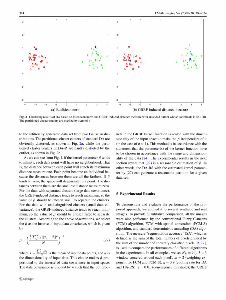
of DA-R with different β . It can be seen that the GRBF-induced distance measure is bounded with monotone in-creasing distance measure zero as ‖xj − vk‖ → 0 and dis-tance measure one as ‖xj − vk‖ → ∞. If ‖xj − vk‖ is largerthan a level (i.e., xj keeps away from vk) then the distancemeasure will be close to its maximum value and give a smallweight K(xj , vk) of xj to vk according to (20). However,the distance measure with the Euclidean norm presents astraight line. That means GRBF-induced distance measureis robust against outliers (i.e., the points which are far awayfrom the main body of the data points) to some extent. Incontrast, the Euclidean distance norm is investible to be sen-sitive to outliers. The robustness of GRBF-induced distancemeasure is demonstrated in Fig. 2, where an outlier is added

Fig. 1 The distance measure plot for the GRBF-induced distance mea-sure with different value of β . The Euclidean norm presents a straightline


(a) Euclidean norm (b) GRBF-induced distance measure

Fig. 2 Clustering results of DA based on Euclidean norm and GBRF-induced distance measure with an added outlier whose coordinate is (0; 100).The partitioned cluster centers are marked by symbol �

to the artificially generated data set from two Gaussian dis-tributions. The partitioned cluster centers of standard DA areobviously distorted, as shown in Fig. 2a; while the parti-tioned cluster centers of DA-R are hardly distorted by theoutlier, as shown in Fig. 2b.

As we can see from Fig. 1, if the kernel parameter β tendsto infinity, each data point will have no neighborhood. Thatis, the distance between each point will attach its maximumdistance measure one. Each point become an individual be-cause the distances between them are all the farthest. If β

tends to zero, the space will degenerate to a point. The dis-tances between them are the smallest distance measure zero.For the data with separated clusters (large data covariance),the GRBF-induced distance tends to reach maximum, so thevalue of β should be chosen small to separate the clusters.For the data with undistinguished clusters (small data co-variance), the GRBF-induced distance tends to reach mini-mum, so the value of β should be chosen large to separatethe clusters. According to the above observations, we selectthe β as the inverse of input data covariance, which is givenby

β =( 1

n

∑Nj=1 ‖xj − x̄‖2

N

)−1

(27)

where x̄ =∑N

j=1 xj

Nis the mean of input data points, and n is

the dimensionality of input data. This choice makes β pro-portional to the inverse of data covariance in input space.The data covariance is divided by n such that the dot prod-

ucts in the GRBF kernel function is scaled with the dimen-sionality of the input space to make the β independent of it(in the case of n > 1). This method is in accordance with thestatement that the parameter(s) of the kernel function haveto be chosen in accordance with the range and dimension-ality of the data [24]. The experimental results in the nextsection reveal that (27) is a reasonable estimation of β . Inother words, the DA-RS with the estimated kernel parame-ter by (27) can generate a reasonable partition for a givendata set.

5 Experimental Results

To demonstrate and evaluate the performance of the pro-posed approach, we applied it to several synthetic and realimages. To provide quantitative comparison, all the imageswere also performed by the conventional Fuzzy C-means(FCM) algorithm, FCM with spatial constraints (FCM-S)algorithm, and standard deterministic annealing (DA) algo-rithm. The measure “segmentation accuracy” (SA), which isdefined as the sum of the total number of pixels divided bythe sum of the number of correctly classified pixels [9, 27],is used to compare the performances of different algorithmsin the experiments. In all examples, we set NR = 9 (a 3 × 3window centered around each pixel), m = 2 (weighing ex-ponent for FCM and FCM-S), η = 0.9 (cooling rate for DAand DA-RS), ε = 0.01 (convergence threshold), the GRBF


Fig. 3 Segmentation results ofdifferent clustering algorithmson synthetic image

Table 1 The values of segmentation accuracy and the centers of classified clusters of six methods on synthetic image

FCM DA FCM-S DA-RS DA-R DA-RS-R

Segmentation accuracy 93.98% 93.88% 98.74% 99.44% 95.07% 99.38%

Classified centers (46.54, 99.23, (54.15, 102.45, (49.95, 100.16, (50.28, 100.21, (49.26, 99.47, (50.16, 100.20,

152.14, 204.27) 153.64, 201.32) 149.72, 199.20) 149.63, 199.62) 149.72, 200.76) 149.69, 199.85)

kernel parameter β is computed by equation (27), the para-meters c (cluster number4 and α (the neighbors effect term)will be given inside the examples. We test the four methods(FCM, FCM-S, DA, DA-RS) on three data sets. The first oneis a set of synthetic images, the second one is a set of simu-lated MR images, and the last one is a set of real images. Allexperiments are performed on P 4 PC with 1.9 G CPU and256 Mb RAM in MATLAB environment.

5.1 Example 1: Synthetic Images

Figure 3a shows a noisy synthetic image. This image con-tains four-class patterns with originally central intensity val-ues (50,100,150,200) (the true ground image is shown inFig. 3b), corrupted by hybrid “Gaussian” and “pepper &salt” noise. This image was constructed so that it would bedifficult to be classified by non-spatially constrained cluster-ing algorithms, such as FCM and DA, as shown in Fig. 3cand Fig. 3d; FCM-S algorithm obtains much better result

4The determination of optimal cluster number is not the focus of thispaper, we assume it is known as a priori in all experiments. Interestedreader could refer to [28] for the discussions of this issue.

but still lacks enough robustness, as shown in Fig. 3e; incontrast, the proposed DA-RS almost completely succeedsin classifying the data, as shown in Fig. 3f. Here we setc = 4 and α = 5.0, the computed value of β from (27) isβ∗ = 0.33 × 10−3. Table 1 gives the numerical results of thefour (plus DA-R and DA-RS-R) methods on the syntheticimage. From the figure and table, it is obvious that the spa-tially constrained algorithms perform much better than non-spatially constrained algorithms, and the proposed DA-RSobtains the best result compared to others. To show the ad-vantage of GRBF-induced distance measure over Euclid-ean distance measure, the result of DA-R is also given inTable 1. Though the SA value of DA-R algorithm is onlyslightly better than DA algorithm, however, the classified in-tensity centers (49.26,99.47,149.72,200.76) of DA-R us-ing GRBF-induced distance are very close to the uncor-rupted cluster centers (50,100,150,200); in contrast, theclassified intensity centers obtained by DA using Euclid-ean distance are (54.15,102.45,153.64,201.32), which areobviously distorted by noise. This observation is in accor-dance with the theoretical analysis in the last section. Fig-ure 4 shows the segmentation accuracy of DA-RS with vary-ing values [1/6 1/5 1/4 1/3 1/2 1 2 3 4 5 6] ×


β∗ of the kernel parameter β for the synthetic image, itcan be seen that the computed β∗ = 0.33 × 10−3 is lo-cated in the optimal range (SA = 99.44), which reveals thatthe inverse of input data covariance is a good estimationfor β .

There are three common types of noise in digital cameraor film image: random noise, “fixed pattern” noise and band-ing noise. To show the performance of the proposed methodon different types of noisy images, we corrupt the true syn-thetic image (Fig. 3b) by each type of the above noise. The

Fig. 4 Segmentation accuracy of DA-RS on synthetic image withvarying values of β

generated images5 are shown in Fig. 5. Table 2 gives theSA values by applying the four (plus DA-R and DA-RS-R)methods on each of the corrupted image. Here the same set-ting c = 4 and α = 5.0 is used, and the individual value ofβ is calculated from equation (27) for each of the images. Itcan be seen that the proposed DA-RS is suitable for all typesof noisy images tested. And the performance of DA-RS isthe best on all of the corrupted images when compared toother methods.

5.2 Example 2: Simulated MR Images

The simulated MR images are obtained from the Brain-Web Simulated Brain Database [25, 26]. Simulated braindata of varying noise are used to perform quantitative as-sessment of the proposed algorithm since ground truths areknown for these data. Here in our experiments, we use ahigh-resolution T1-weighted phantom with slice thicknessof 1 mm, varying levels of noise and no intensity inhomo-geneities.6 The raw MR images with varying (3%, 5%, 7%,and 9%) levels of noise are shown in Fig. 6. And Fig. 7shows the discrete true partial volume models7 of CSF, GM

5The random noise is simulated by Gaussian white noise with mean 0and variance 0.005; the “fixed pattern” noise is simulated by “salt &pepper” noise with noise density 0.1; and the banding noise is gener-ated by polluting every three lines of the image.6The proposed algorithm is developed generally for robust segmenta-tion of all kinds of images but not limited to MR images. We don’tdiscuss the inhomogeneities issue in the current paper. Some of themethods in the literature, especially the one in [9], can be directly com-bined into the proposed algorithm to reduce the inhomogeneities effectin MR image segmentation. Please refer to Appendix 2 for details.7The true partial volume models are available at http://www.bic.mni.mcgill.ca/brainweb/anatomic_normal.html

Fig. 5 Different types of noisyimages generated by corruptingthe true ground synthetic imageusing different types of noise

Table 2 Segmentation results of six methods on different types of noisy images


Random noise 86.60% 86.46% 98.67% 99.51% 89.27% 99.37%

Fixed pattern noise 93.45% 93.45% 96.33% 99.37% 95.01% 99.24%

Banding noise 92.73% 92.96% 98.82% 99.54% 94.39% 99.52%


Fig. 6 The raw MR image with varying levels of noise

Fig. 7 The true partial volumemodels of CSF, GM and WMfor the simulated MR image

and WM tissues those were used to generate the simulatedMR image. The number of tissue classes in the segmentationwas set to three, which corresponds to gray matter (GM),white matter (WM) and cerebrospinal fluid (CSF). Back-ground and other tissues are ignored in the computation.The image with 9% noise is investigated in details in thisexperiment. Figure 8 shows the CSF, GM and WM mem-bership (probability) functions obtained by applying FCM,DA, FCM-S and DA-RS, respectively. All the membership(probability) functions are scaled from 0 to 255. Here weset α = 0.85, and the computed value of β from (27) isβ∗ = 2.20 × 10−3. It can be seen that because of the noiseeffect presents in the data, the performances of both FCMand DA are seriously deteriorated. In contrast, spatially con-strained methods obtain much better results, with DA-RSachieving a slightly more robustness than FCM-S. Table 3gives the segmentation accuracy (SA) of CSF, GM and WMby using the four (plus DA-R and DA-RS-R) algorithms onthe same image. Similarly, the DA-RS method shows muchbetter result than FCM and DA and slightly better result thanFCM-S on this highly noisy image.

In addition, Table 4 shows the overall SA values obtainedby applying all the different algorithms to the same MR im-age with different levels of noise (see the images in Fig. 6).As expected, an increase in the level of noise always leadsto a decrease in the SA values for all methods. However,the DA-RS method is most robust against increased noise. It

also can be observed that FCM and DA perform quite wellfor low levels of noise but the performances rapidly degradeas noise is increased.

5.3 Example 3: Real Images

In this example, we test the proposed algorithm on sev-eral real images. The segmentation results of the proposedDA-RS and another three methods (DA, FCM, FCM-S) onthese real images are plotted here for qualitative compar-isons. The quantitative comparisons can’t be provided cur-rently since the ground truth of the tested real images doesnot exist.

The first real image, as shown in Fig. 9a, is the Riceimage from Image Processing Toolbox, MathWorks. WhiteGaussian noise with mean 0 and variance 0.05 has beenadded to the image. The goal is to extract the rices from thebackground. So we set c = 2 for this image. The segmenta-tion results of FCM and DA are shown in Fig. 9b and Fig. 9c,respectively, it is obvious that these results are distorted bythe noise. In contrast, FCM-S and DA-RS with α = 1 obtainmuch better results as shown in Fig. 9d and Fig. 9e, these re-sults are hardly distorted by the noise. It also can be seen thatthe result of DA-RS is slightly better than that of FCM-S.

The second real image, as shown in Fig. 10a, is the MRimage provided by Dr. Shen, School of Medicine, Univer-sity of Pennsylvania. White Gaussian noise with mean 0 and


Fig. 8 CSF, GM and WMmembership (probability)functions of different clusteringalgorithms on the simulated MRimage with 9% noise

Table 3 Segmentation accuracy of CSF, GM and WM by applying five methods on simulated MR image with 9% noise


CSF 92.68% 91.74% 93.55% 93.10% 92.31% 93.06%

GM 85.41% 79.29% 90.48% 91.41% 85.66% 91.42%

WM 87.59% 92.93% 95.46% 96.63% 93.32% 96.07%

Overall 87.61% 87.99% 93.43% 94.27% 89.82% 93.99%


Table 4 Segmentation accuracy obtained by applying different methods on simulated MR image with varying levels of noise


3% noise 96.64% 96.61% 96.83% 96.88% 96.69% 96.83%

5% noise 94.92% 94.93% 95.78% 96.06% 95.12% 95.99%

7% noise 92.07% 92.35% 95.08% 95.62% 93.82% 95.43%

9% noise 87.61% 87.99% 93.43% 94.27% 89.82% 93.99%

Fig. 9 The segmentation results of four methods on the real Rice image

Fig. 10 The segmentation results of four methods on the real MR image

variance 0.001 has been added to the image. The goal isto segment the image into gray matter (GM), white matter(WM), cerebrospinal fluid (CSF), and background. So weset c = 4 for this image. Similarly, the FCM-S (as shownin Fig. 10d) and DA-RS (as shown in Fig. 10e) algorithmswith α = 1 obtain much better results than FCM (as shownin Fig. 10b) and DA (as shown in Fig. 10c), with DA-RSachieving a slightly better performance than FCM-S does.

From the above observations, we can say that the pro-posed DA-RS algorithm has the best segmentation perfor-mance on the tested real images when compared to otherexisting segmentation methods.

5.4 Computation Time Comparison

It is obviously that DA-R needs more execution time thanDA due to the injection of the GRBF-induced distance mea-sure, and DA-RS needs more execution time than DA-Rdue to the computation of spatial information. Typically, DAruns 2–5 times faster than DA-R and DA-R runs 5–10 time

faster than DA-RS. Table 5 gives the comparison of the run-ning time in the above three experiments by using FCM,FCM-S, DA, DA-R, DA-RS, and DA-RS-R. It can be seenthat FCM type algorithms run a little faster than accordingDA type algorithms. Fortunately, the DA-RS-R algorithm,the complexity reduced version of DA-RS algorithm, sig-nificantly reduces the execution time, and runs even muchfaster than FCM-S algorithm, as shown in the last column inthe table.

6 Investigation on Spatial Strength

The proper selection of the spatial penalty parameter α isimportant for obtaining optimal or near-optimal image seg-mentation performance. When α is set to zero, the spatially-constrained algorithm is equivalent to the non-spatially-constrained algorithm, while α approaches too larger, theblurring phenomenon may occur. Determination of an ap-propriate value of α is dependent on the image being clus-tered. Theoretically, the relative importance of the regular-


Table 5 Execution time of six different methods on the above three examples

FCM FCM-S DA DA-R DA-RS DA-RS-R

Example 1, Fig. 3 3.89 s 77.96 s 7.20 s 15.20 s 154.72 s 21.93 s




izing term (determined by α) is inversely proportional tothe signal-to-noise (SNR) ratio of the observed image. LowSNR would require a higher value of α, and vice versa.However, in practical cases, SNR may not be known as apriori, which makes the selection of α difficult. In the litera-ture, few attempts have been presented to deal with it. To thebest of our knowledge, only [5] so far discussed the adaptiveselection of α by using a cross-validation method, however,that method suffers from extreme computation cost, whichmakes it be impractical in real applications. Here we pre-liminarily investigate a simple but efficient method for theadaptive selection of the spatial penalty parameter.

As observed from a real image, homogeneous pixels arenormally clustered together such that the intensity value xj

of a given image pixel j is normally similar to the valuesof its neighbor pixels, that means the variance of the givenimage pixel xj against its neighbors is small. While if thegiven image pixel is contaminated, the variance becomeslarge. From this observation, we select the spatial strengthαj for each image pixel j by the scaled standard deviationas follows,

αj = λj/λ̄ (28)

where λj is the standard deviation8 of xj against its neigh-bors, which is defined by

λj =√√√√

1

NR

∑

r∈Nj

‖xr − xj‖2 (29)

and λ̄ is the mean of the standard deviation of all pixels,which is defined by

λ̄ = 1

N

N∑

j=1

λj (30)

where Nj stands for the set of neighbors falling into a (nor-mally 3×3) window around xj (not including xj ) and NR isits cardinality. From (28), the value of αj can be calculated

8The definition here is a little different from the formally mathe-

matic one, which is defined by λj = ( 1NR

∑r∈Nj

‖xr − μ‖2)12 with

μ = 1NR

∑r∈Nj

xr

directly from the given image itself, which is computation-ally practical in really applications. However, in the formu-lation of DA-RS, the spatial penalty parameter is presentedby uniform α, but not dynamic αj , to apply the above selec-tion method (28), we need to modify the distance definitionof DA-RS as follows,

D′′kj = (1 − K(xj , vk)) + αj

NR

∑

r∈Nj

(1 − K(xr , vk)). (31)

In the above definition, the spatial penalty term of imagepixel j is regularized by the parameter αj . Note unlike thestandard spatially-constrained methods, where all the pixelsare regularized by a uniform parameter α as in (21). Whilethey are regularized by dynamical values αj in (31), which isadaptively selected by the scaled standard deviation of eachpixel against its neighbors by using (28).

To apply DA-RS with the standard distance defini-tion (21), we need to pre-determine a proper value for thespatial penalty parameter α, which may be impractical inreal applications. However, by using the new distance defin-ition (31), the dynamic spatial penalty parameter αj is adap-tively selected by (28), which makes DA-RS more practicalin applications. What is more, using the dynamic spatialpenalty parameter αj for the individual image pixel xj canlead to a better segmentation accuracy when compared to thestandard formulation. Table 6 and 7 show the comparativeresults of DA-RS by using different distance definitions, i.e.,(21) and (31), on the synthetic and simulated MR images,respectively. It can be seen that the performance of DA-RSis increased by using the dynamic spatial penalty parameterαj when compared to the uniform spatial penalty parame-ter α. It also indicates that (28) is a reasonable estimation ofthe spatial penalty parameter αj .

7 Conclusion

In this paper, we have proposed a modified deterministic an-nealing algorithm that can perform unsupervised clusteringfor robust image segmentation. The key to the algorithm is anew dissimilarity measure that takes into account the influ-ence of the neighboring pixels on the center pixel in a 3 × 3window based on a (GRBF-induced) robust non-Euclidean


Table 6 Comparative results of DA-RS by using uniform α and dynamic αj on synthetic images with different types of noise

Fig. 3a Fig. 5a Fig. 5b Fig. 5c

Uniform α 99.44% 99.51% 99.37% 99.54%

Dynamic αj 99.89% 99.96% 99.90% 99.93%

Table 7 Comparative results of DA-RS by using uniform α and dynamic αj on simulated MR images with different levels of noise

Fig. 6a Fig. 6b Fig. 6c Fig. 6d

Uniform α 96.88% 96.06% 95.62% 94.27%

Dynamic αj 97.10% 96.32% 95.81% 94.49%

distance measure. The superiority of the proposed algo-rithm over standard image segmentation algorithms has beendemonstrated by experimental results on synthetic and realimages. The main contributions of this paper could be sum-marized as follows: 1) Extend the DA algorithm for imagesegmentation by combining two robust techniques, i.e., non-Euclidean distance and local spatial regularity, and thereforeachieve better segmentation performance compared to ex-isting methods in the literature. 2) The proposed scheme isgeneral, which can be applied to other fuzzy or probabil-ity clustering algorithms to achieve their corresponding ro-bust versions. What is more, the proposed scheme is simplebut efficient, which can be easily reproduced by the inter-ested readers. 3) Work out efficient methods to adaptivelyselect suitable values for GRBF kernel parameter and spatialstrength parameter. These methods are also general, whichcan be applied to other kernel-based algorithms and spatiallyconstrained algorithms.

Acknowledgements The authors sincerely thank the anonymous re-viewers for their insightful comments and valuable suggestions on anearlier version of this paper.

Appendix 1: Critical Temperature for Phase Transition

Deterministic Annealing begins by determining the mini-mum of the free energy at high values of T and attemptsto track the minimum through lower values of T , until theglobal minimum of the free energy at T → 0 coincides withthe global minimum of the original cost function. During theannealing in T it is observed, that the cluster center remainsat the mass center of the related cluster up to a critical value.At that point the representation undergoes a transition andthe cluster center splits up in feature space [16, 29]. Thesesplits are related to qualitative changes in the optimizationproblem and have to be taken into account in the anneal-ing process. In order to avoid wasting computation time oneshould start the annealing at an initial value Tini > T ∗, whereT ∗ is the value at which the first split in the representation

occurs. The variational calculus of free energy with respectto perturbed cluster centers yields a critical value T ∗ for thefirst phase transition in terms of the largest eigenvalues ofcovariance matrix [16]

T ∗ = 2λmax(Cφ(x)) (32)

where Cφ(x) is the kernel-induced covariance matrix

Cφ(x) = 1

N

N∑

j=1

φ̄(xj )φ̄(xj )T (33)

of centered images

φ̄(xj ) = φ(xj ) − 1

N

N∑

i=1

φ(xi) (34)

of the data points. The calculation of eigenvalue of Cφ(x) isextremely not practical due to the high or infinite dimen-sional of feature space. From singular value decomposi-tion (SVD) it can be seen that the matrix of dot productsDφ(x) with elements Dij = 1

Nφ̄(xi)φ̄(xj )

T has the samenonzero eigenvalues as Cφ(x) [29]. Thus λmax(Cφ(x)) =λmax(Dφ(x)), where Dφ(x) can be calculated using

Dij = 1

Nφ̄(xi)φ̄(xj )

T

=[K(xi, xj ) − 1

N

N∑

p=1

K(xp, xi)

− 1

N

N∑

q=1

K(xq, xj ) + 1

N2

N∑

p,q=1

K(xp, xq)

]. (35)

During the annealing process, the data keeps splitting un-til the given cluster number c reaches. Assume the givendata are split into Γ (c > Γ > 1) clusters (denoted byC1, . . . ,Cγ , . . . ,CΓ ) in a certain temperature, then the crit-


ical temperature T ∗γ for the γ th (1 ≤ γ ≤ Γ ) cluster phase

transition can be calculated by the maximum eigenvalue ofthe conditional kernel-induced covariance matrix of the γ thcluster

Cφγ (x) =N∑

j=1

p(φ(xj )|φγ (x))(φ(xj )

− φγ (x))(φ(xj ) − φγ (x))T (36)

where p(φ(xj )|φγ (x)) is obtained through the Bayes for-mula

p(φ(xj )|φγ (x)) = p(φ(xj ))p(φγ (x)|φ(xj ))

p(φγ ). (37)

Due to the high or infinite dimensional of feature space, theeigenvalues of Cφγ (x) can be approximately calculated fromthe matrix of dot products Dφγ (x) with elements Di,j∈Cγ ofthe γ th cluster, which is given by

Di,j∈Cγ = 1

Nγ

φ̄γ (xi)φ̄γ (xj )T

=[K(xi, xj ) − 1

Nγ

∑

p∈Cγ

K(xp, xi)

− 1

Nγ

∑

q∈Cγ

K(xq, xj ) + 1

N2γ

∑

p,q∈Cγ

K(xp, xq)

]

(38)

where Nγ is the number of data points in the γ th cluster,then we get the approximate critical temperature for phasetransition of the γ th cluster, that is

T ∗γ = 2λmax(Dφγ (x)). (39)

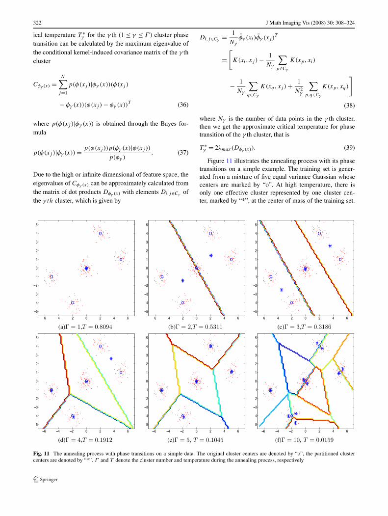
Figure 11 illustrates the annealing process with its phasetransitions on a simple example. The training set is gener-ated from a mixture of five equal variance Gaussian whosecenters are marked by “o”. At high temperature, there isonly one effective cluster represented by one cluster cen-ter, marked by “*”, at the center of mass of the training set.

Fig. 11 The annealing process with phase transitions on a simple data. The original cluster centers are denoted by “o”, the partitioned clustercenters are denoted by “*”. Γ and T denote the cluster number and temperature during the annealing process, respectively


As the temperature is lowered, the system undergoes phasetransitions which increase the number of effective clustersas shown in Fig. 11.

Appendix 2: Bias Field in MR Images

The observed MR signal Y can be modeled as a product ofthe true signal X generated by the underlying anatomy, anda spatially varying factor G called the gain field

Yj = XjGj ∀j ∈ 1,2, . . . ,N (40)

where Xj and Yj are the true and observed intensities at thej th pixel, respectively, Gj is the gain field at the j th pixel,and N is the total number of pixels in the MR image. Theapplication of a logarithmic transformation to the intensitiesallows the artifact to be modeled as an additive bias field [30]

yj = xj + bj ∀j ∈ 1,2, . . . ,N (41)

where xj and yj are the true and observed log-transformedintensities at the j th pixel, respectively, and bj is the biasfield at the j th pixel. If the gain field is known, then it is rel-atively easy to estimate the tissue class by applying a con-ventional intensity-based segmenter to the corrected data.Similarly, if the tissue classes are known, then we can es-timate the gain field. But it may be problematic to estimateeither without the knowledge of the other. We will show be-low that by using an iterative algorithm, the deterministicannealing (DA) (for discussion simplification, same schemecan be applied to DA-RS) algorithm can estimate both.

Substitute the equation (41) into the probability function(8) and free energy function (9) of standard DA algorithm,we have

p(vk|(yj − bj )) = pk exp− dkj

T∑ci=1 pi exp− dij

T

(42)

and

Fb = −T

N∑

j=1

p(yj − bj ) logc∑

i=1

pi exp−dij

T(43)

where p(yj − bj ) is the prior distribution of yj − bj , dkj =‖yj − bj − vk‖2 is the distance measure between yj − bj

and vk , and pk = ∑Nj=1 p(xj )p(vk|(yj − bj )) is the mass

probability of the kth cluster.Taking the derivatives of Fb with respect to vk and bj ,

and setting the results to zero we get

vk =∑N

j=1 p(yj − bj )p(vk|(yj − bj ))(yj − bj )∑N

j=1 p(yj − bj )p(vk|(yj − bj ))(44)

and

bj = yj −∑c

k=1 p(yj − bj )p(vk|(yj − bj ))vk∑ck=1 p(yj − bj )p(vk|(yj − bj ))

. (45)

By using the iterative updating equations (42), (44) and (45),the DA algorithm can estimate and correct the bias fieldvalue for each pixel in the image, such that reduce the biasfield effect in the image segmentation.

References

1. Pal, N.R., Pal, S.K.: A review on image segmentation techniques.Pattern Recognit. 26(9), 1277–1294 (1993)

2. Bezdek, J.C., Hall, L.O., Clarke, L.P.: Review of MR image seg-mentation techniques using pattern recognition. Med. Phys. 20,1033–1048 (1993)

3. Pham, D.L., Xu, C., Prince, J.L.: Current methods in medical im-age segmentation. Annu. Rev. Biomed. Eng. 2, 315–337 (2000)Palo Alto, CA

4. Bezdek, J.C.: Pattern Recognition with Fuzzy Objective FunctionAlgorithms. Plenum, New York (1981)

5. Pham, D.L.: Spatial Models for Fuzzy Clustering. Comput. Vis.Image Underst. 84, 285–297 (2001)

6. Liew, A.W.C., Yan, H.: An adaptive spatial fuzzy clustering algo-rithm for 3-D MR image segmentation. IEEE Trans. Med. Imaging22(9), 1063–1075 (2003)

7. Tolias, Y.A., Panas, S.M.: On applying spatial constraints in fuzzyimage clustering using a fuzzy rule-based system. IEEE SignalProcess. Lett. 5(10), 245–247 (1998)

8. Tolias, Y.A., Panas, S.M.: Image segmentation by a fuzzy clus-tering algorithm using adaptive spatially constrained membershipfunctions. IEEE Trans. Syst. Man Cybern. 28(3), 359–369 (1998)

9. Ahmed, M.N., Yamany, S.M., Mohamed, N., Farag, A.A., Mori-arty, T.: A modified fuzzy C-means algorithm for bias field esti-mation and segmentation of MRI data. IEEE Trans. Med. Imaging21(3), 193–199 (2002)

10. Liew, A.W.C., Leung, S.H., Lau, W.H.: Fuzzy image clusteringincorporating spatial continuity. Inst. Elec. Eng. Proc. Vis. ImageSignal Process. 147(2), 185–192 (2000)

11. Liew, A.W.C., Leung, S.H., Lau, W.H.: Segmentation of color lipimages by spatial fuzzy clustering. IEEE Trans. Fuzzy Syst. 11(4),542–549 (2003)

12. Zhang, D.Q., Chen, S.C.: A novel kernelized fuzzy C-means al-gorithm with application in medical image segmentation. Artif.Intell. Med. 32, 37–50 (2004)

13. Zhang, D.Q., Chen, S.C.: Robust image segmentation using FCMwith spatial constraints based on new kernel-induced distancemeasure. IEEE Trans. Syst. Man Cybern. 34(4), 1907–1916(2004)

14. Vovk, U., Pernus, F., Likar, B.: MRI intensity inhomogeneitycorrection by combining intensity and spatial information. Phys.Med. Biol. 49, 4119–4133 (2004)

15. Rose, K., Gurewitz, E., Fox, G.C.: Statistical mechanics and phasetransitions in clustering. Phys. Rev. Lett. 65(8), 945–948 (1990)

16. Rose, K.: Deterministic annealing for clustering, compression,classification, regression, and related optimization problems. Proc.IEEE 86(11), 2210–2239 (1998)

17. Rajagopalan, A.N., Jain, A., Desai, U.B.: Data clustering usinghierarchical deterministic annealing and higher order statistics.IEEE Trans. Circuits Syst. II: Analog Digit. Signal Process. 46(8),1100–1104 (1999)


18. Rose, K., Gurewitz, E., Fox, G.C.: Constrained clustering as an op-timization method. IEEE Trans. Pattern Anal. Mach. Intell. 15(8),785–794 (1993)

19. Dave, R.N., Krishnapuram, R.: Robust clustering methods: a uni-fied view. IEEE Trans. Fuzzy Syst. 5(2), 270–293 (1997)

20. Yang, X.L., Song, Q., Wu, Y.L.: A robust deterministic anneal-ing algorithm for data clustering. Data Knowl. Eng. 62(1), 84–100(2007)

21. Cristianin, N., Shawe-Taylar, J.: An Introduction to Support Vec-tor Machines and Other Kernel-Based Learning Methods. Cam-bridge University Press, Cambridge (2000)

22. Müller, K.R., Mike, S., Rätsch, G., Tsuda, K., Schölkopf, B.:An introduction to kernel based learning algorithms. IEEE Trans.Neural Netw. 12(2), 181–201 (2001)

23. Schölkopf, B., Smola, A.J.: Learning with Kernels. MIT Press,Cambridge (2002)

24. Schölkopf, B., Burges, C.J.C., Vapnik, V.: Extracting support datafor a given task. In: Fayyad, U.M., Uthurusamy, R. (eds.) Ist Int.Conf. on Knowledge Discovery and Data Mining, pp. 252–257.AAAI Press, Menlo Park (1995)

25. McGill University, Canada [Online]. Available: http://www.bic.mni.mcgill.ca/brainweb

26. Cocosco, C.A., Kollokian, V., Kwan, R.K.S., Evans, A.C.: Brain-Web: online interface to a 3D MRI simulated brain database. Neu-roImage 5(4), S245 (1997)

27. Pham, D.L., Prince, J.L.: Adaptive fuzzy segmentation of mag-netic resonance images. IEEE Trans. Med. Imaging 18(9), 737–752 (1999)

28. Yang, X.L., Song, Q., Cao, A.Z.: A new cluster validity index fordata clustering. Neural Process. Lett. 23(3), 325–344 (2006)

29. Graepel, T., Obermayer, K.: Fuzzy topographic kernel clustering.In: Brauer, W. (ed.) Proceedings of the 5th GI Workshop FuzzyNeuro Systems, pp. 90–97 (1998)

30. Wells, W.M., Grimson, W.E.L., Kikinis, R., Jolesz, F.A.: Adaptivesegmentation of MRI data. IEEE Trans. Med. Imaging 15(4), 429–442 (1996)

Xu-Lei Yang received the B.E. degree and M.E.degree from EE School, Xi’an Jiaotong Uni-versity in 1999 and 2002, respectively. He ob-tained the PhD degree from EEE School, NTUin 2005. His current research interests includepattern recognition, image processing, and ma-chine vision. He has published more than 20papers in scientific book chapters, journals andconference proceedings.

Qing Song received the B.S. and the M.S. de-grees from Harbin Shipbuilding Engineering In-stitute and Dalian Maritime University, Chinain 1982 and 1986, respectively. He obtained thePhD degree from the Industrial Control Centerat Strathclyde University, U.K in 1992. He iscurrently an associate professor and an activeindustrial consultant at the school of EEE, NTU.His research interests focus on a few compu-tational intelligence related research programs

targeted for practical applications.

Yue Wang received his Bachelor degree fromWuhan University, China, and the Master andPh.D. degrees in Electrical and Electronic En-gineering from Nanyang Technological Univer-sity, Singapore. He is currently working as a se-nior researcher in Institute for Infocomm Re-search, Singapore. He has published many pa-pers in scientific journals and conference pro-ceedings. His research interests include com-puter vision and pattern recognition, object seg-

mentation and matching, biomedical image processing, spline approx-imation and deformable model.

Ai-Ze Cao received the B.S. degree in BeijingInstitute of Technology in 1993, M.S. degreein Changchun Institute of Optics and Fine Me-chanics, Chinese Acad. SCS. in 1996, and PhDdegree in EEE School, NTU in 2005, respec-tively. She is now a research fellow in med-ical center, Vanderbilt University. Her currentresearch interests include data clustering, imagesegmentation, and medical image analysis.

Yi-Lei Wu received his Bachelor degree fromFudan University, China, and the Ph.D. degreesin Electrical and Electronic Engineering fromNanyang Technological University, Singapore.He is currently working as a R&D Engineer inSeagate Technology International Pte Ltd, Sin-gapore. His research interest is the robust analy-sis of recurrent neural network and gradientbased learning algorithms.

a modified deterministic annealing algorithm for robust image segmentation

Documents