-1-

A Long Run Pure Variance Common Features Model for the Common Volatilities of the Dow Jones

Robert F. Engle Department of Finance, New York University, Leonard N. Stern School of Business

and

Juri Marcucci*

Department of Economics, University of California, San Diego

August, 2004

Abstract In this paper a new model to analyze the comovements in the volatilities of a portfolio is

proposed. The Pure Variance Common Features model is a factor model for the

conditional variances of a portfolio of assets, designed to isolate a small number of

variance features that drive all assets’ volatilities. It decomposes the conditional variance

into a short-run idiosyncratic component (a low-order ARCH process) and a long-run

component (the variance factors). An empirical example provides evidence that models

with very few variance features perform well in capturing the long run common

volatilities of the equity components of the Dow Jones.

Keywords: Common Features, Pure Variance Common Features, Factor Models, Factor

ARCH, Canonical Correlations, Reduced Rank Regression.

JEL Codes: C52, C32

* Corresponding author: E-mail: jmarcucc@weber.ucsd.edu.

-2-

1 INTRODUCTION

In finance there is a strong belief that movements in the price of one particular asset are

quite likely to coincide with movements in the prices of other assets, possibly quoted in different

markets. These comovements might be caused by the reaction of economic agents to particular

changes in some macroeconomic and financial variables or, maybe, to specific news about the

company or about the economic sectors involved. In addition, the movements in one asset price

may have implications that are likely to affect the value of other assets either contemporaneously

or with some lags. This behavior has traditionally been modeled with factor models in which

asset prices are driven by a small number of latent variables called factors and others named

idiosyncratic disturbances. The concept of factors plays a crucial role in two major asset pricing

theories: the mutual fund separation theory of which the standard Capital Asset Pricing Model

(CAPM) is a special case and the Arbitrage Pricing Theory (APT) of Ross (1976, 1978).

Typically these models are linear and are identified by the assumption that all these latent

variables are independent. Their aim is to seek a data reduction by specifying a small number of

latent variables that influence a large number of output variables.

Common Features (CF hereafter), introduced by Engle and Kozicki (1993), is a further

generalization of these concepts. A small number of latent variables, with a specific

characteristic or feature, influence all the observables and give them this feature, with respect to

which, the problem becomes of smaller dimension and more tractable. By associating the factors

with such features, it is possible to build factor style models for much more general situations.

In many cases, these factor models can be formulated as reduced rank regressions or canonical

correlation problems. The most widely used example of CF and the main motivation for the idea

is cointegration, the phenomenon where a reduced number of common stochastic trends can

determine the long run properties of a large number of observables (Granger, 1983, Engle and

Granger, 1987). There are many approaches to estimation and testing for the number of unit

roots, but the most popular are based on reduced rank regression and on canonical correlations,

as in Johansen (1988) and Ahn and Reinsel (1990). Many other types of CF’s have been

examined in the literature, such as serial correlation CF’s (Vahid and Engle, 1993 and 1997)

which are called common cycles in macroeconomics and risk premiums in finance, common

seasonals (Engle and Hylleberg, 1996, Cubadda, 1999), common non-linearities (Anderson and

-3-

Vahid, 1998), or common structural breaks (Hendry and Mizon, 1998). In particular, there are a

few CF’s that examine the structure of the second moments of a set of variables such as common

ARCH factors (Engle and Susmel, 1993), common persistence (Bollerslev and Engle, 1993), or

common long-range dependence (Ray and Tsay, 2000). All these structures have the potential

and in some cases the realized benefit of improving the performance of large models by

restricting the number of parameters to ensure that such features are common.

Traditionally, since the seminal papers by Engle (1982) and Bollerslev (1986), volatility

is modeled with univariate ARCH/GARCH models. Nevertheless, since the beginning of this

burgeoning literature both financial econometricians and practitioners have understood the

importance of multivariate GARCH models because the finance practice needs to handle the risk

involved in big (if not huge) portfolios. Among these Multivariate GARCH models, the most

important are the VECH model of Bollerslev, Engle and Wooldridge (1988), the Constant

Conditional Correlation (CCC) model of Bollerslev (1990), the Factor ARCH model of Engle,

Ng, and Rothschild (1990), and Ng, Engle and Rothschild (1992), the BEKK model by Engle

and Kroner (1995), or the more recent Dynamic Conditional Correlation (DCC) model of Engle

(2002).

The typical difficulty with these models is the number of parameters required to specify

large covariance matrices. Many of the important simplifications are factor models – such as the

Factor ARCH models of Engle, Ng, and Rothschild (1990) or the conditionally heteroskedastic

latent factor models of Diebold and Nerlove (1989). Intuitively, the Factor ARCH model

assumes that there are few factors or portfolios (i.e. linear combinations of the observed random

variables) whose time-varying variances drive the whole covariance matrix of the system. On

the other hand, the conditionally heteroskedastic latent factor model of Diebold and Nerlove

(1989) is a traditional statistical factor analysis model, with a diagonal idiosyncratic covariance

matrix, in which the variances of the common factors are parameterized as univariate ARCH

processes. Sentana (1998) highlights the basic differences between these two models. The

covariance matrix of the Factor ARCH model is by construction measurable with respect to the

usual information set that contains only past values of the observables, while the conditionally

heteroskedastic latent factor model can be regarded as a stochastic volatility model.

Furthermore, another distinctive feature is related to the implicit definition of the factors which is

completely different between the two models. In conditionally heteroskedastic latent factor

-4-

models the factors capture the comovements between the observed series, whereas in Engle, Ng

and Rothschild’s (1990) Factor ARCH model the factors are directly related to those linear

combinations of the observed series which summarize the comovements in their conditional

variances. King, Sentana and Wadhwani (1994) generalize the Diebold and Nerlove’s (1989)

model by constructing a multivariate factor model that nests the latter, in which time-varying

volatility of returns is induced by the changing volatility of the underlying factors, that can be

observable or unobservable. A great advantage of their model is not only a parsimonious

representation of the conditional variance-covariance matrix of excess returns as a function of

the changing variances of a small set of factors, but also the easier identification of these factors

in this context. Actually, Sentana and Fiorentini (2001) show how identification problems in

factor models with conditional heteroskedasticity can be easily solved when variation in factor

variances is accounted for in the estimation.

In this paper we suggest a new type of CF’s. A Pure Variance Common Features (PVCF)

is a statistical model that describes how the conditional variances of a collection of assets may all

depend upon a small number of variance factors. This differs from the factor models described

above in that it does not require that the covariances also depend on these same factors. This is

precisely the problem that the risk manager of an options portfolio faces, and is also a central

feature of measuring risk in standard portfolio problems. The second extension of the volatility

factor models is that the idiosyncracies are allowed to have short run variability. The factors

explain common movements in long run volatilities. The existence of such common components

implies that the relationships between the volatilities are tied together in the long run, and

therefore are interpretable as long run equilibrium relationships. As with other types of CF’s, we

should be able to obtain superior volatility forecasts by using the fact that there exist few

common volatility components (or pure variance common features). Furthermore, the presence

of few common volatility components can have important implications for asset pricing

relationships and in optimal portfolio allocations. The price of an asset typically depends on the

conditional variance with some benchmark portfolio. Therefore, the pricing of long term

contracts may be completely different from that of one-period contracts if there are common long

run volatility components in the conditional variance or in the covariance with the benchmark

portfolio. Last but not least, the pricing of certain portfolios of assets can be more sensitive to

these long run volatility components than to the idiosyncratic short run volatility components.

-5-

The plan of the rest of the paper is as follows. Section 2 illustrates the options portfolio

problem that motivates the model. Section 3 introduces the Pure Variance Common Features

model that should be useful in building big models and managing portfolios of options. Section

4 develops the econometric specification and the problems involved in the detection of common

long run volatility components. The empirical relevance of the PVCF model is discussed in

Section 5 where an application to the thirty stocks of the Dow Jones Industrial Average Index is

presented. The PVCF model seems to perform rather well by identifying two or three pure

variance common features that affect all the volatilities. Section 6 concludes giving also

directions for further research.

2. MEASURING THE RISK OF AN OPTIONS PORTFOLIO

Risk managers, options traders and strategists must understand the risk of an options

portfolio. In general, this would include options with several strikes, different maturities and

various underlying assets. By invoking some variant of Black Scholes option pricing, it is easy

to evaluate the risk of portfolios of options with a single underlying asset. In this fashion,

options traders aim to reduce risk by holding portfolios that are both delta and vega neutral, so

that they are approximately unaffected by small movements in the underlying asset price and in

its volatility. With multiple underlyings, only the deltas are typically evaluated.

Consider a collection of options whose prices at time t are given by a vector pt. The

price of the underlying assets, arranged in the same fashion, is given by st and the volatilities of

these assets can be stacked into a vector vt. Some of these volatilities will be the forecast

volatility over a short horizon while others will be over a long horizon. For many volatility

models, these will simply be proportional.

The delta of this portfolio of options is defined by

'

tt

t

ps∂∆ =∂

(1)

Most elements of this matrix are zero since the price of an option on one asset will be

unaffected by a change in the value of another underlying asset price as long as the first is

-6-

unchanged. There may be additional parameters in delta, and each of these must be evaluated at

the time the hedge or risk measure is undertaken; for example, the estimate at t-1 would be

written 1t t−∆ . A portfolio with w dollars in each position would be valued at 1 't t tw pπ −= . To

make this portfolio delta neutral, offsetting positions would be taken in the underlying assets to

give portfolio value

( )1 1't t t t t tw p sπ − −= − ∆ (2)

This portfolio has no risk for small movements in any of the components of tp .

When volatility changes the option prices will change. The vega of the vector of options

is defined as:

'

tt

t

pv∂Λ =∂

(3)

Again, this would be expected to be a block diagonal matrix. Since the derivative of ts

with respect to tv is zero, the vega of the delta neutral portfolio in (2) is

1 / 1''

tt t t

t

wvπ

− −∂ = Λ∂

(4)

where | 1t t−Λ denotes the estimate of tΛ at 1t − . By the chain rule, the derivative with respect to the conditional variance is

11 / 12

1 '2

tt t t t

t

w Dvπ −

− −∂ = Λ∂

(5)

where 2

tv is the vector of conditional variances and Dt is the diagonal matrix of conditional

standard deviations. If we denote 1 1 2t tw w− −= and the variance covariance matrix of the

volatilities can be forecast as

( )21t t tVar v− ≡ Ψ (6) then the portfolio variance is given by:

-7-

( ) 1 1

1 1 / 1 / 1 1' 't t t t t t t t t t tVar w D D wπ − −− − − − −= Λ Ψ Λ (7)

Only if ' 0w Λ = , will this portfolio not be dependent on the covariance matrix of

volatilities. This can be achieved by balancing the volatility exposure with respect to each of the

underlyings. Often, this is not possible, leading to a need for a covariance matrix of the

volatilities of the underlyings. This expression gives quantitative meaning to the sense in which

a short volatility position in one asset can be hedged by a long volatility position in another. If

the volatilities are highly correlated then the risk will be small.

The focus of the paper is on developing expressions for the covariance of asset volatilities

as indicated in equation (6). From the expression, it appears that this is the forecast of the

volatility over the next day, however from the development, it should be clear that this is a

forecast of the volatility over the remaining life of an option, so it will generally be many days or

even years. For long horizon forecasts, the volatility of the volatility becomes very small as the

new information has a relatively small effect on the long run forecasts.

In the next section, a factor model will be introduced for the conditional

variances. This will provide a method for calculating the conditional covariance matrix among a

set of volatilities.

3. THE PVCF MODEL

An important problem in a wide range of financial applications is the modeling of the

variance covariance matrix of a high number of assets. This requires estimation not only of the

variances, but all the covariances. The Factor ARCH model introduced by Engle, Ng, and

Rothschild (1990) parameterizes this matrix in terms of a small set of factors with time-varying

variances. Although there are data sets where one or two factors describe the entire covariance

matrix, this might not always be the case.

Instead, we can look for common features that only affect the variances. The first step in

many approaches for the estimation of a covariance matrix is to estimate the univariate

variances, as in Engle’s (2002) DCC model. While it is possible to estimate many variances

separately, as if they were independent series, there may be relations between these variances

-8-

that can and should be exploited. Frequently, simple GARCH models of a collection of assets

show remarkable similarities possibly due to the presence of common volatility processes.

While a full model of portfolio allocation and Value at Risk will require estimating the

correlations, a closely related problem will depend dramatically on the relations between the

variances.

Consider a vector of asset excess returns, Ntr ∈ , with conditional mean vector tµ . To

simplify the notation consider the 1N × vector -t t tr r µ= corrected to have mean zero by

subtracting the conditional mean vector1. Then, construct a vector of the squares of these returns

denoted 2t t tr r r= where represent the Hadamard (or element by element) product. Such a

vector would be equivalent to the vector of the 't tdiag rr , where ( )diag A represents a column

vector extracted from the main diagonal of the matrix A . Based on a sigma field of past values

of all returns ( )1t−ℑ , the problem is to specify and estimate the full variance-covariance matrix:

( )1t t t t t tV r H D R D− ≡ = (8) or the single conditional variances ( ) 2 2

1t t t t tE r h diag H diag D− ≡ = = (9) where tH is the covariance matrix of tr , tD is the diagonal matrix of conditional standard

deviations and tR is the correlation matrix.

A pure variance common features (PVCF) model for this problem can be formulated as a

linear factor model for the conditional variances of tr

t t th diagξ= Γ + Ω (10)

1 We can also consider a more general setting where tµ is a vector of time-varying risk premia, related to the factors

that drive the return process. As explained later in the paper, considering tµ as a linear combination of factor risk premia, the PVCF model can be translated into an APT framework. However, the focus of the paper is on isolating common volatilities and we leave further analyses exploring this more general model for future work.

-9-

where tξ is a 1K × vector of positive random variables (called variance factors), Γ is an N K×

matrix of variance factor loadings, and tΩ is an N N× diagonal positive semi-definite matrix of

idiosyncratic variances that in the literature are usually assumed to be constant. The variance-

covariance matrix of this vector of variances can be directly evaluated from (10) when the

idiosyncratic covariance matrix is constant

( ) ( )1 1 1 1 't t t tV h V ξ− + − += Γ Γ (11) Notice that ht is given as a function of information at time t-1, but the value of ht+1 is a random

variable with a covariance matrix as summarized above.

This formulation is closely related to the CAPM and APT asset pricing models as well as

to the Factor ARCH model. An APT model with K factors can be expressed as

( )1, ' 0t t t t t tr f E fη η−= Γ + = (12) where returns and factor returns are interpreted as excess returns. The covariance matrix of this

vector of returns is

( ) ( ) ( )1 1 1' ,t t t t t t t tV r V f V η− − −= Γ Γ +Ω ≡ Ω (13) If the idiosyncratic covariance matrix is time invariant, then all variances and covariances of

returns will depend only on the covariance matrix of the factors. If, in addition, the factors are

conditionally uncorrelated, then the variances of the factors will be the only state variables.

Thus, the common features described in (10), are the factor variances. The covariances among

volatilities will depend on the variance-covariance matrix of the conditional variances as in (11).

If idiosyncratic volatilities are not constant, then there will be time variation in th beyond

that explained by the factors. For most asset management functions, transitory changes in

volatilities can be ignored. Thus, if the idiosyncratic volatilities are mean reverting at a rapid

rate, then the model can be treated as a factor model. We here introduce the idea of a long run

pure variance common feature (LRPVCF), which is closely related to the concept of

copersistence suggested by Bollerslev and Engle (1993). It allows the possibility of short run

volatility in the idiosyncrasies.

-10-

We assume a low order ARCH process for the idiosyncratic variances. These

assumptions guarantee that each element of tdiag H is positive and can be written as

20 ,

1

J

t it i t i ij i t jiij

H h rγ ξ α α −=

= = + +∑ (14)

where iγ is the i -th row of Γ , a simple ARCH(p) model is assumed for the idiosyncratic

variances, tξ is a vector of K positive variance factors, and the ikα ’s are non-negative

parameters. In addition, it is expected that K N , or, alternatively, that the number of variance

factors which drive the comovements in the conditional variances of the whole portfolio is quite

small.

An alternative useful formulation of the additive model in (10) is a vector multiplicative

model such as

* *expt t th diagξ = Γ + Ω (15)

where, ( )* logt tξ ξ= , and *

tΩ is the Exponential ARCH equivalent of the matrix tΩ . With this

multiplicative formulation, the logarithm of the conditional covariance matrix has now a factor

structure. Each element of the main diagonal of the conditional covariance matrix can therefore

be written as

( ) , ,*0 1/ 2 1/ 2

1 1, ,

log .p p

i t j i t jt it i t i ij ijii

j ji t j i t j

r rH h

h hγ ξ α α δ− −

= =− −

= = + + +∑ ∑ (16)

The LRPVCF model considers also time-varying idiosyncratic volatilities with low

persistence and, therefore, it is not possible to construct portfolios with constant conditional

variances as in the Factor ARCH model.

Usually, one of the main purposes in building a new model is to have better multiperiod

forecasts. In the additive PVCF model the multiperiod forecasts of the conditional variances in

the main diagonal of tH can be calculated as follows

-11-

( ) ( ) ( )t t t t t tE diag H E E diagτ τ τξ+ + += Γ + Ω (17)

where the variance factors t τξ + are forecastable through the model adopted to get the factors

themselves, while the idiosyncratic variances are forecastable from a low order ARCH process.

The τ −period ahead forecast for the i − th asset’s conditional variance will be

( ) 2, 0 ,

1

p

i t i t t i t ij i t jj

h E E rτ τ τγ ξ α α+ + + −=

= + +

∑ (18)

For long horizon forecasts the last term is constant, leaving the volatility process as an exact

factor model. A parallel forecast for the multiplicative form is similar, but requires some

distributional assumptions.

4 ECONOMETRIC SPECIFICATION AND ESTIMATION

To complete the econometric specification of the LRPVCF model we must specify the

joint distribution of the factors and the returns. The easiest specification is when the factors are

observables. The underlying factors may be the conditional variances of observable indices

such as the Dow Jones, the S&P500 or the NASDAQ. In this case, the volatility of these indices

is estimated with a univariate GARCH model and in each case an asymmetric component model

is chosen. In some versions of the model, the observed implied volatility of the S&P500 as

measured by the new VIX index is used instead of the GARCH volatility of the underlying. This

version of the model is called Market PVCF (PVCF-MKT) model.

Assuming joint conditional normality both for the returns and the factors, we can write

the full model as:

1 ~ 0,'

t t t t tt

t t t

r D R D GN

f G F−

ℑ

(19)

where

-12-

2 20

1

p

t t t j t jj

diag D h rξ ω ω −=

≡ = Γ + +∑ (20)

and 2

0 1 1 2 1t t t tdiag F fξ θ θ θ ξ− −≡ = + + (21) so that the conditional variance of returns depends upon the conditional variance of the factors.

The model is written using vectors of parameters and simple models. The multiplicative model

simply replaces equation (20) with (16). The generalization to an asymmetric component model

for the factors and to an asymmetric model for the idiosyncrasies is straightforward.

Maximum Likelihood estimation would involve also specifying the process for the

correlations among the variables and the covariances with the factors. Instead, the moment

conditions associated with estimation of merely the variance equations are considered. This is

therefore a GMM or QMLE type of estimation. We will apply a two step estimation strategy.

First the parameters of equation (21) are estimated. Then (21) is substituted into (20) and the

remaining parameters are estimated based on the first step parameters. The Quasi Likelihoods

for each step are the same.

( ) ( ) 21 , ,

1 1

1 log /2

T K

k t t k tt k

QL fθ ξ ξ= =

= − + ∑∑ (22)

( ) ( ) 22 , , ,

1 1

1, log /2

T N

i t i t i tt i

QL h r hω= =

Γ = − + ∑∑ (23)

Since the correlations are not estimated in either case and the joint likelihood is never

used, this is a precise example of Newey and McFadden (1994)’s two-step GMM estimator.

They present formulae for the standard errors of the two-step estimator but we have not yet

implemented these.

The factors can also be extracted directly from the returns data rather than using

observable indices. We have applied two approaches: principal components and canonical

correlations, and one hybrid which is principal components of a collection of observed sector

returns.

The principal components approach is a slight variation of the Orthogonal GARCH

model suggested by Alexander (2001) denoted PVCF-PC. An approach close to this is used in

the Factor ARCH context by Engle and Ng (1993). The volatilities of the first K principal

-13-

components of the returns are estimated using the Component ARCH model of Engle and Lee

(1999) where K is the number of variance features.

In the second approach, the variance features are given by the exponential of the first K

canonical variates between the logarithmic squared returns and their most recent past. This is the

Canonical Correlation PVCF model (PVCF-CC). To motivate this approach, define the squared

returns as the variances times the residuals

2 2t t tr h e= (24)

Taking logs of both sides and adding a very small constant (ϖ ) to deal with exact zeros in

recorded returns and approximating the logarithm of the conditional variance in terms of lagged

squared returns in logarithms, a logarithmic p-th order ARCH, the equation becomes:

( ) ( ) ( )

( ) ( )

2 2

2 2

1

log log log

log log

t t t

p

j t j tj

r h e

r e

ϖ

α ϖ−=

+ +

+ +∑

(25)

The canonical correlation procedure seeks linear combinations of the right hand side

variables that are maximally correlated with linear combinations of the left hand side variables.

Thus, the linear combinations of the past squared returns in logarithm, which are highly

correlated with their current values, may be a good choice of variance factors. The exponentials

of the first K canonical variates are treated as pure variance common features.

The hybrid approach is the Sector PVCF model (PVCF-SEC), where the variance factors

are given by the univariate GARCH volatilities of the largest principal components of the

average returns of all economic sectors of the Dow Jones.

Once the PVCF model is estimated, we can employ a set of diagnostic tests for assessing

its validity. The first battery of tests involves the portmanteau test for residual autocorrelation in

the squared standardized residuals given by equation (24). Such tests are equation by equation

in spirit and give information about the left over residual autocorrelation for each single squared

return.

Another set of specification tests that can be used is the battery of multivariate tests first

introduced by Ding and Engle (2001), in which the orthogonality of the models’ residuals is

-14-

tested. For a well specified PVCF model, the squared standardized residuals could not be

forecast based on any other past information in the model. Ding and Engle (2001) indicate three

consequences of correct model specification: A1) ( )'t t TE e e I= , A2) ( )2 2, 0jt itCov e e = , for all

i j≠ , and A3) ( )2 2,, 0it j t kCov e e − = , for 0k > . Because in the PVCF models the correlations

between the variables are not jointly modeled, tests of adequacy can only be based on A3). The

null hypothesis in A3) is equivalent to the moment condition ( )1 0tE m = , where 1tm is a N2

vector with typical element 2 2, 1it j te e − . The empirical moments ( )1 1 1

1ˆˆ ˆT

T ttm T m θ−

== ∑ should be

close to zero if such condition holds.

Relying on the results of Newey (1985) and Tauchen (1985) for conditional moment

testing in a Maximum Likelihood context, Ding and Engle (2001) suggest several specification

tests. These tests are designed to test whether moment conditions of the form

( ) ( )1 2 2 2 2

, , 1ˆ ˆ ˆ ˆ ˆij t it i j t jm e e e e−= − − (26)

are satisfied by the model.

Letting 1tm be the T k× matrix of conditional moments, under fairly general conditions

we have that ( )1/ 2 1' 0,dtT i N− → Ωm , where i is a 1T × vector of ones. Therefore, the

covariance tests by Ding and Engle (2001) can be viewed as Lagrange Multiplier tests, whose 2uTR statistics (where 2

uR is the uncentered 2R from the auxiliary regression of ones on the

moments) are equivalent to the quadratic form

( ) 11 ˆˆ ˆ' 'T i i−− Ω1 1

t tm m (27)

where 1ˆ 'T −Ω = 1 1

t tm m is a consistent estimator of the covariance matrix of the conditional

moments. However, since the PVCF models are in a QMLE setting, there remains some theory

needed to rigorously establish the distributions of these tests. Actually, the moments might not

be martingale difference sequences as a consequence of the dynamic misspecification induced in

the standardized residuals ite by the use of the conditional variances, instead of the full

-15-

covariance matrix. This is the reason why we might need a robust estimate of Ω to compute all

such tests. We can thus use a non-parametric estimator of the long-run covariance matrix of the

empirical moments which is HAC consistent. A natural candidate is the Newey-West estimator

( )( )1 1

1

ˆ ˆ ˆ ˆ ˆ ˆ ˆ' ' 'q

j jj

T T w q− −− −

=

Ω = + +⌡1 1 1 1 1 1t t t t t tm m m m m m (28)

where ( )w q is the Bartlett kernel and q is a truncation lag. The robust version of the

covariance tests is then given by (27) with Ω replaced by (28). This is the version that will be

adopted for all the covariance tests presented in this paper.

Ding and Engle (2001) suggest testing all of these moments as 1) the Lagged Covariance

test ( LC -test), which is designed to detect time dependency in multivariate time series, whose

test statistic is T times the squared multiple correlation coefficient of the auxiliary regression of

constant unity on the empirical moment 1ˆTm . The typical element of this set of N2 moments is

defined in (26) as the first lagged sample covariances. The LC -test is asymptotically distributed

as a 22Nχ under the null. The other test is 2) the Composite Lagged Covariance test ( 1CLC -test),

whose test statistic is T times the uncentered 2R from the auxiliary regression of 1 on 1ˆTM ,

where the moments are defined as the sum of all the first lagged sample covariances, i.e. 1 1

, ˆ ˆT ij tij

M m=∑ . Such test is asymptotically distributed as a 21χ under the null.

We extend these covariance tests to include more lags and to exclude both the moment

conditions where i j= and those redundant in (26). These tests are 3) the Alternative Lagged

Covariance test ( ALC -test), which is designed to detect time dependence of multivariate time

series only across assets, thus avoiding redundant ARCH testing within the same asset. The test

statistic is similar to the LC -test but for the lagged sample covariances included. In the ALC -

test the ( )1 / 2N N − empirical moments are those in (26) with 1, ,j i N= + … . Its asymptotic

distribution is 2( 1) / 2N Nχ − under the null. The other two tests are devised to detect possible time

dependence at longer lags. They are constructed by adding the moments of the previous tests at

each lag. They are: 4) the Additive Composite Lagged Covariance test at lag k ( kACLC -test)

which is calculated using the k moments of each jCLC -test with lag j that goes from 1 to k .

-16-

5) The Additive Alternative Lagged Covariance test at lag k ( kAALC -test) which is based on

the k sums of the ALC -test moments at each lag from one to k . The asymptotic distribution of

these last two tests under the null is 2kχ . For all these tests to have the correct distribution under

the null of correct specification, they should also include the scores with respect to the estimated

parameters. The omission of these additional regressors will only reduce the value of the test

statistic, leading it to be conservative.

In the next section, these methods will be examined with the portfolio of the thirty equity

returns of the Dow Jones Industrial Average.

5 MODELING COMMON VOLATILITIES IN THE DOW STOCKS: EMPIRICAL

EVIDENCE

5.1 Univariate Statistics

The data we analyze in this paper consist of daily returns2 for the thirty stocks of the Dow

Jones Industrial Average Index for a ten year period from February 20, 1992 to February 20,

2002. For each stock, we have a total of 2609 prices downloaded from Datastream. The Dow

Jones Industrial Average is a price weighted average of the returns on thirty industrial stocks.

The thirty stocks examined in this paper are those that were included in the index in spring 2002.

Table 1 gives a complete list of their ticker symbols, company names and the corresponding

economic sectors. All these stocks are listed on the New York Stock Exchange, except for Intel

and Microsoft that are traded on NASDAQ.

[Insert Table 1 about here]

In Table 2, the univariate statistics for the whole data set in percentage terms are

presented. The mean for each stock return is on average around 0.05%, while the standard

deviation is around 2. Out of the fourteen stock returns considered that show significant

skewness, nine exhibit negative skewness (with bigger values for Boeing, Eastman Kodak and 2 Returns exceeding 20% in absolute value are replaced by the average return over the two most adjacent days. The main reason is that ARCH tests can give low values for the relative statistics, leading to the failure to reject the null hypothesis of no ARCH effects, if the series is characterized by unrepeated ‘big events’. With such big jumps in some of the series, we would certainly obtain low values for the common ARCH tests as well, so that more portfolios would misleadingly fail to reject the null hypothesis of absence of ARCH, even though the single asset volatilities moved differently.

-17-

Honeywell), while all the others display positive skewness almost close to zero. The kurtosis is

always significant and never below 5, thus far away from the normal case of 3. The same

conclusion can be easily inferred from the Jarque-Bera test, which rejects the null of normality

for all returns at any reasonable significance level. Table 2 also shows the Ljung-Box statistics

to test the null hypothesis of absence of serial correlation in both the returns in levels (LB) and in

squares (LB2) until the fifteenth lag. The returns in levels show a certain degree of serial

correlation, since for twenty out of thirty cases, we reject the null. Furthermore, the LB2 test on

the squared returns indicates the presence of serial correlation at any significance level and,

therefore, the existence of ARCH effects. In this case, the theoretical distribution of the LB test

is not correct and there is a tendency to over reject the null.

[Insert Table 2 about here]

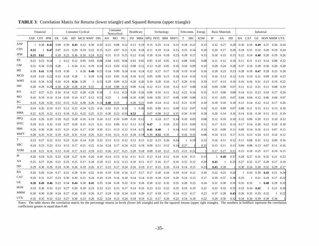
5.2 Correlation Analysis

We also examined the correlation matrix of the thirty returns, both in levels and in

squares, to better understand the possible links among different stocks and their volatilities.

Table 3 shows the correlation matrix for the returns in levels in the lower left triangle and for the

squares in the upper right triangle.

[Insert Table 3 about here]

The stock returns do exhibit positive and significant correlations with each other not only

in the levels, but also in the squares. Out of the 30 correlation coefficients in the levels, 7 are

even higher than 0.50 and, among these, one is bigger than 0.60. Not surprisingly, the strongest

correlations are between stocks within the same industry: American Express and Citigroup,

American Express and JP Morgan, JP Morgan and Citigroup, Wal-Mart Stores and Home Depot,

Microsoft and Intel, Johnson & Johnson and Merck. However, there is also a very strong

correlation between General Electric and American Express which are in different economic

sectors, although the former does have important financial business so that this may not be

surprising.

The correlations between squared returns are naturally related to the correlations between

the levels of returns, but can be helpful to discover possible comovements in their volatilities.

From the upper triangle in Table 2, we can see that there are 7 correlation coefficients above 0.45

and almost all correspond to stocks within the same business area: American Express and JP

-18-

Morgan, JP Morgan and Citigroup, Home Depot and Wal-Mart, International Paper and Alcoa,

Honeywell and General Electric. The other strong correlations outside the same economic sector

are those between General Electric and American Express, and General Electric and Home

Depot. Other correlations (Home Depot and American Express, Honeywell and Boeing) are

quite strong. All these results indicate that there are strong comovements in the volatilities of the

thirty stocks in the Dow Jones. Most of these comovements are within or between specific

industries, showing the possible presence of more than just one volatility factor. In particular,

we can infer the existence of industry specific volatility factors together with a global or market

factor3.

5.3 ARCH Tests and Univariate GARCH estimates

Table 4 reports some ARCH tests. These are Lagrange Multiplier (LM) tests with

univariate information sets. Each return is squared and used as a proxy for the realized volatility.

Then, each squared return is regressed on a constant and 4, 8 and 12 lags of the same squared

return. The statistic is obtained by multiplying the uncentered 2R from this regression by the

sample size, and asymptotically is distributed as a 2pχ where p is the number of lags.

[Insert Table 4 about here]

We thus find strong evidence of ARCH effects at any lag, for all stocks. These results

are corroborated by the univariate GARCH estimates for each stock return, which are highly

significant for all the thirty assets examined and are not reported for the sake of brevity.

Figure 1 displays annualized volatilities for nine of the thirty assets, as estimated from

individual univariate GARCH. We report the annualized volatilities for only few stocks, because

others resemble volatility patterns that are similar to the ones presented. Nevertheless, the

volatility patterns seem to be quite different among the thirty assets of the Dow, indicating that

there might be more than one volatility factor which drives all these volatilities.

[Insert Figure 1 about here]

3 These correlation results do not change if we adopt a sort of preprocessing of the returns, such as fitting individual AR processes or a VAR.

-19-

5.4 Testing for Common ARCH Features

Since all stock returns in the Dow Jones show ARCH effects, we test for the presence of

common ARCH features, following the Engle and Susmel’s (1993) pairwise methodology.

Whenever two series display ARCH effects, we test for common ARCH features (or factor

ARCH), by seeking those linear combinations for which this feature is not present. In fact, we

look for those portfolio weights for which the variance of the whole portfolio only depends on

the volatilities of the idiosyncrasies. The test is implemented by minimizing the usual LM

ARCH test over the cofeature vector. If tx and ty have both ARCH effects, we minimize the

ARCH test for t t tw x yδ= − with respect to δ . The procedure involves a regression of 2tw

against lagged squared values of both series and their cross products, followed by the

minimization of 2TR over the parameter δ . This is a general method-of-moment-type of test

and under suitable assumptions it follows a 2χ distribution with degrees of freedom equal to the

number of overidentifying restrictions (see Engle and Kozicki, 1993). Engle and Susmel (1993)

look for the minimum by performing a grid search. In the present paper we use both a grid

search and the BFGS (Broyden-Fletcher-Goldfarb-Shanno) method4, but the final results do not

change considerably.

We carry out the test for common ARCH features on the squared returns and out of the

435 possible two-asset portfolios, only 4 pairs show a common ARCH feature, at the usual 5%

significance level. We also perform other kinds of testing along the same line. We minimize the

ARCH LM test for combinations of various net returns, by subtracting from each series the

return on some market indices, such as S&P500 and NASDAQ. We adopt the same testing

procedure by including in the portfolios either the S&P500 or the NASDAQ, and by looking for

common ARCH features among three-asset portfolios. The main conclusion is that the

preceding results still hold: only very few portfolios show a common ARCH feature.

This finding is not completely new in the literature: Alexander (1995) finds no-ARCH

portfolio for any exchange rate pairs, using daily data from a ten-year sample of dollar returns on

seven currencies and from some of its sub-samples. Her main conclusions are twofold: firstly

daily data contain so much noise that it is really hard to find a common feature. Secondly, the

Engle-Kozicki test might have reduced power in a dynamic setting. This latter line of argument 4 The BFGS is a quasi-Newton optimization method that does not imply the calculation of the Hessian matrix of the objective function.

-20-

follows Ericsson’s (1993) critique to Engle and Kozicki (1993). Ericsson argues that, in a

bivariate setting, the cofeature hypothesis might be too restrictive, and, consequently, it could be

rejected, even if the cofeature does exist. To solve this problem it would be sufficient using

multivariate procedures, in such a way to include in the information set all the lagged data and

not only the lags for the pair of variables under investigation.

As a matter of fact, we select two sub-samples from our data set, and run the same

common factor ARCH tests. Again and not surprisingly, very few pairs fail to reject the null of

no ARCH effects, leading to the rejection of a common ARCH feature.

When the same test is run on the logarithmic transformation of squared returns plus a tiny

constant to make the transformed series closer to being normally distributed, the results turn out

to be much more encouraging5, because more evidence of common features is found. Actually,

almost all the portfolios exhibit a common ARCH feature, since only for 35 pairs out of 435 the

null of no ARCH effects is rejected. The interpretation of such common features is however

different.

A further explanation for the difficulties in finding common ARCH factors is closely

related to the assumed factor structure. As Engle and Susmel (1993) point out, if the

idiosyncratic components in the model do not have a constant covariance matrix, there will be no

portfolio that shows a constant variance-covariance matrix, because even though one can find a

coefeature vector that annihilates the matrix of factor loadings, there will still be a time-varying

volatility component, due to the idiosyncrasies, that cannot be diversified.

Thus, in the next section we will look for possible long run pure variance common

features, taking into account the fact that the idiosyncrasies seem to exhibit ARCH-like time-

varying volatilities. This fact implies the presence of variance features that are common to more

than just a pair of asset returns and calls for a more general search that must necessarily be

multivariate.

5.5 How Many Pure Variance Common Features are in the Dow?

Figure 1 illustrates how individual GARCH annualized volatilities seem to display very

different patterns. This means that there is more than one pure variance factor driving the whole

5 For brevity we do not report the corresponding tables that are available upon request from the authors.

-21-

volatility process of the Dow Jones Industrial Index. As argued before, one variance factor can

be related to the market, but there is evidence of the possible presence of industry specific

variance factors.

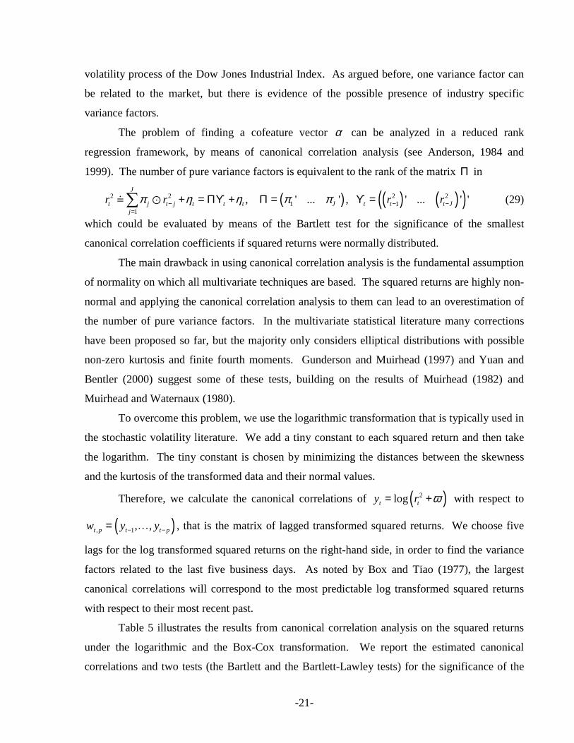
The problem of finding a cofeature vector α can be analyzed in a reduced rank

regression framework, by means of canonical correlation analysis (see Anderson, 1984 and

1999). The number of pure variance factors is equivalent to the rank of the matrix Π in

( ) ( ) ( )( )2 2 2 21 1

1, ' ... ' , ' ... ' '

J

t j t j t t t J t t t Jj

r r r rπ η η π π− − −=

+ = Πϒ + Π = ϒ =∑ (29)

which could be evaluated by means of the Bartlett test for the significance of the smallest

canonical correlation coefficients if squared returns were normally distributed.

The main drawback in using canonical correlation analysis is the fundamental assumption

of normality on which all multivariate techniques are based. The squared returns are highly non-

normal and applying the canonical correlation analysis to them can lead to an overestimation of

the number of pure variance factors. In the multivariate statistical literature many corrections

have been proposed so far, but the majority only considers elliptical distributions with possible

non-zero kurtosis and finite fourth moments. Gunderson and Muirhead (1997) and Yuan and

Bentler (2000) suggest some of these tests, building on the results of Muirhead (1982) and

Muirhead and Waternaux (1980).

To overcome this problem, we use the logarithmic transformation that is typically used in

the stochastic volatility literature. We add a tiny constant to each squared return and then take

the logarithm. The tiny constant is chosen by minimizing the distances between the skewness

and the kurtosis of the transformed data and their normal values.

Therefore, we calculate the canonical correlations of ( )2logt ty r ϖ= + with respect to

( ), 1, ,t p t t pw y y− −= … , that is the matrix of lagged transformed squared returns. We choose five

lags for the log transformed squared returns on the right-hand side, in order to find the variance

factors related to the last five business days. As noted by Box and Tiao (1977), the largest

canonical correlations will correspond to the most predictable log transformed squared returns

with respect to their most recent past.

Table 5 illustrates the results from canonical correlation analysis on the squared returns

under the logarithmic and the Box-Cox transformation. We report the estimated canonical

correlations and two tests (the Bartlett and the Bartlett-Lawley tests) for the significance of the

-22-

first k-1 canonical correlation coefficients, k=1,…,p, with the corresponding degrees of freedom

and p-values. The null hypothesis is equivalent to ( ) 1rank kΓ = − , where 122 21−Γ = Σ Σ is the

matrix of regression coefficients of ty on ,t pw .

[Insert Table 5 about here]

There is no practical difference between the two sequential tests, and the number of pure

variance factors found is two for the logarithmic transformation and three for the Box-Cox. If

more lags are taken for the right hand side variables ,t pw , only the first canonical correlation

remains significant for the log transformed squared returns, while the previous results still hold

for the Box-Cox transformation.

5.6 Estimating the Long Run Pure Variance Common Feature Model for the Dow

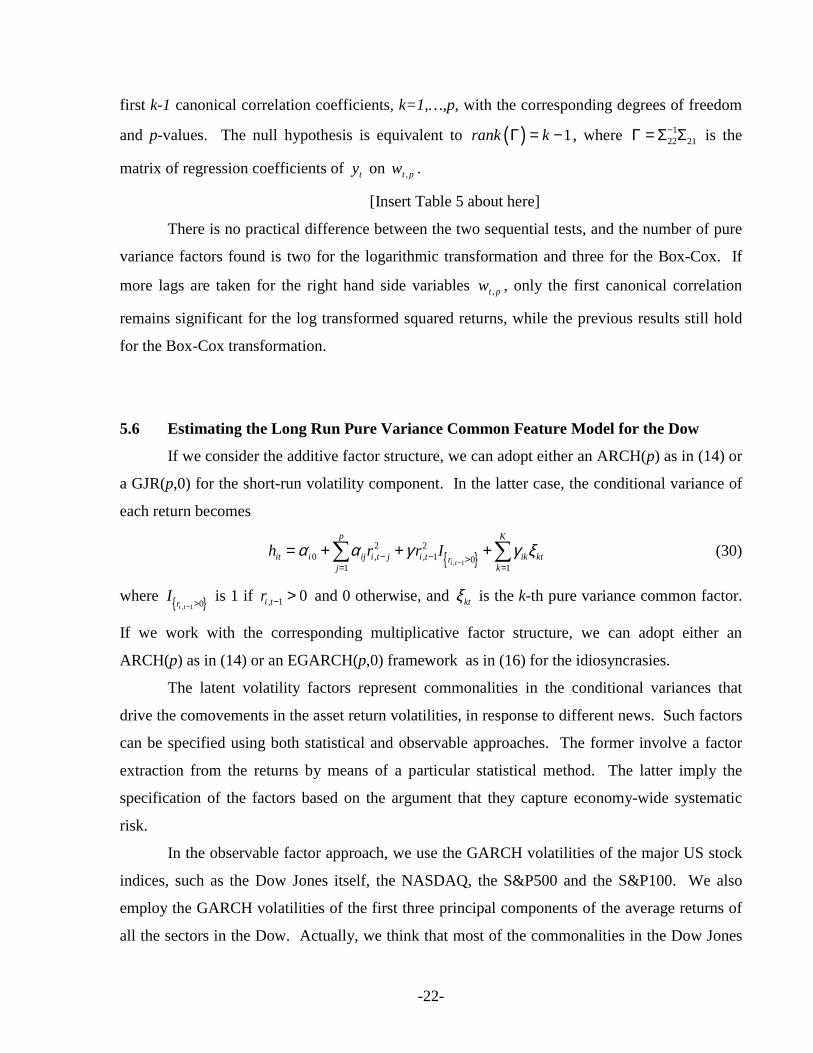
If we consider the additive factor structure, we can adopt either an ARCH(p) as in (14) or

a GJR(p,0) for the short-run volatility component. In the latter case, the conditional variance of

each return becomes

, 1

2 20 , , 1 0

1 1i t

p K

it i ij i t j i t ik ktrj k

h r r Iα α γ γ ξ−

− − >= =

= + + +∑ ∑ (30)

where , 1 0i trI− >

is 1 if , 1 0i tr − > and 0 otherwise, and ktξ is the k-th pure variance common factor.

If we work with the corresponding multiplicative factor structure, we can adopt either an

ARCH(p) as in (14) or an EGARCH(p,0) framework as in (16) for the idiosyncrasies.

The latent volatility factors represent commonalities in the conditional variances that

drive the comovements in the asset return volatilities, in response to different news. Such factors

can be specified using both statistical and observable approaches. The former involve a factor

extraction from the returns by means of a particular statistical method. The latter imply the

specification of the factors based on the argument that they capture economy-wide systematic

risk.

In the observable factor approach, we use the GARCH volatilities of the major US stock

indices, such as the Dow Jones itself, the NASDAQ, the S&P500 and the S&P100. We also

employ the GARCH volatilities of the first three principal components of the average returns of

all the sectors in the Dow. Actually, we think that most of the commonalities in the Dow Jones

-23-

volatilities are linked not only to these key US stock market indices, but also to the different

economic sectors of the Dow.

All PVCF models are estimated by quasi maximum likelihood, treating the factors

estimated in a first step as given. For each model we calculate the principal components of the

estimated conditional volatilities. This is a descriptive statistic designed to measure how closely

the volatilities move together. For example, in a one factor PVCF model with constant

idiosyncratic volatility, the first principal component would explain all the variability, since all

volatilities would move proportionally to each other. With increased idiosyncratic volatility, the

proportion of all volatility explained by the first factor would decline. Other factors would also

contribute, so the explanatory proportion due to the second and third principal component would

reveal the importance of additional factors. Furthermore, the Ljung-Box test for the squared

standardized residuals up to the fifteenth lag is evaluated to assess how much serial correlation

(and hence ARCH effect) is left on each residual. For each PVCF model five covariance tests

are also computed to assess temporal dependence left in the residuals of the whole multivariate

model.

Tables 6 and 7 give a summary of these tests for all the PVCF models estimated. For

each model, the tables show the cumulative variance explained by the first four principal

components, the covariance tests that each model passes, and the number of assets (out of thirty)

for which we fail to reject the null of absence of serial correlation in the squared standardized

residuals until the fifteenth lag. The tables exhibit these results for the models with statistical

factors (PVCF-PC and PVCF-CC) and those with variance factors from the market indices and

from the economic sectors (PVCF-MKT and PVCF-SEC). Five robust covariance tests ( LC ,

ALC , kCLC , kACLC and kAALC tests) up to the fifth lag are evaluated for each model using

HAC robust standard errors for the empirical moments as in (28), where an automatic truncation

lag is adopted. However, we report only those robust tests passed by each model. The CLC-

tests at higher lags are constructed using the k-th dimensional vector of empirical moments given

by the sum of the sample covariances from lag 1 to k. One possible problem with the LC and

ALC tests is the high number of degrees of freedom (900 and 435 respectively with 30N = ) for

which the asymptotic theory may not work properly. Consequently, in commenting the results,

we put more emphasis on the other covariance tests.

-24-

The variance explained by the first principal component of the conditional volatilities is

quite high (always greater than 40%), but the next principal components can hardly explain the

5%, suggesting that there is no need for additional variance factors. The Ljung-Box test for the

squared standardized residuals (LB2) indicates that the PVCF-PC models capture most of the

individual ARCH effects in each asset. When the number of lags taken for the ARCH process of

the idiosyncratic volatilities is high almost every return can pass the LB2 test.

[Insert Tables 6 and 7 here]

Combining the different criteria shown in Tables 6 and 7 and looking at those models that

pass most of the covariance tests, we select the best model within each PVCF model. The

EGARCH(5,0)-3PC is the best PVCF-PC model, while the GJR(5,0)-1CC and the GARCH(5,0)-

2SEC outperform all the others in the PVCF-CC and PVCF-SEC class, respectively. The

GJR(5,0)-SPNQ turns out to be the best model among those that employ market variance factors.

All these models are characterized by the highest number of acceptances for the LB2 test, and the

highest proportion of explained variance. In addition, the EGARCH(5,0)-3PC model seems to a

certain extent superior among the best models in terms of number of covariance tests passed.

However, no model can clearly beat the others. In terms of number of variance features, the

PVCF-CC model is the only one for which one variance factor is sufficient to characterize the

comovements in the volatilities of the Dow. The additive model both with symmetric or

asymmetric GARCH for the idiosyncratic volatilities seems to perform better than the

multiplicative model. Actually, the PVCF models with GARCH and GJR processes for the

transitory volatility component pass the covariance tests more often than those with EGARCH.

Tables 8 through 11 give the estimated parameters for the best model in each class of PVCF

model. Only the estimates for the long-run volatility components are presented.

Table 8 exhibits the parameter estimates for the GJR(5,0)-SPNQ model with two

variance factors given by the GARCH volatilities of the S&P500 and NASDAQ indices. For

almost all assets in the Dow, the variance factors are highly significant. Moreover, the model

rejects the null of absence of serial correlation in the squared standardized residuals up to the

fifteenth lag only for few assets (Johnson & Johnson, SBC Communications and Wal-Mart

Stores). The GJR(5,0)-SPNQ model does not pass the LC, ALC and CLC tests at the first lag

and ACLC at the second lag at any reasonable significance level. Instead, it passes the CLC-

-25-

tests at the second through the fourth lag at the 5%, the CLC at the fifth, the ACLC at the third

and the AALC at the second lag at the 1%.

[Insert Table 8 about here]

Table 9 shows the results for the EGARCH(5,0)-3PC model with three variance factors

given by the Component ARCH volatilities of the first three principal components of the returns.

For most returns, the volatility factors are significant and there is some degree of serial

correlation left in the squared standardized residuals, because we fail to reject the null up to the

fifteenth lag for all the assets but Johnson & Johnson, McDonalds, SBC Communications and

Wal-Mart Stores. The EGARCH(5,0)-3PC model cannot pass the LC and the ALC tests at any

level of significance. However, it passes the CLC-test from the first up to the fifth lag and all the

ACLC and AALC tests at the 5%. Thus, the model shows evidence of adequacy in capturing the

common volatilities in the thirty stocks of the Dow Jones.

[Insert Table 9 about here]

Table 10 illustrates the estimates for the GJR(5,0)-1CC model with just one variance

feature given by the exponential of the canonical variate associated with the largest canonical

correlation between the log transformed squared returns and their most recent past. The

volatility factor is highly significant for all stock returns. Seven stocks (Alcoa, American

Express, General Electric, Johnson & Johnson, Coca Cola, SBC Communications, and Wal-Mart

Stores) show evidence of residual serial correlation in the squared standardized returns. The

GJR(5,0)-1CC model cannot pass either the LC, the ALC and the CLC tests at first and third lag

or all the additive tests. Nevertheless, it passes the CLC-tests at the second, fourth and fifth lag

at the usual 5% significance level.

[Insert Table 10 about here]

Table 11 exhibits the estimates for the GARCH(5,0)-2SEC model with two variance

factors given by the GARCH volatilities of the first two principal components of the returns of

the Dow Jones’ sectors. Only few stocks present estimates for the factor volatilities that are not

significant. Some serial correlation in the squared standardized residuals can be found only in

Alcoa, Johnson & Johnson, SBC Communications and Wal-Mart Stores. The GARCH(5,0)-

2SEC model does not pass the LC, the ALC, and the CLC tests at the first lag at any reasonable

significance level. However, it passes the CLC-tests at the second through the fourth lag and the

-26-

AALC at all lags at the 5%. It also passes the CLC at the fifth lag and the ACLC at all lags at

1%.

[Insert Table 11 about here]

Figure 2 depicts the factors and the corresponding volatility factors obtained from

Canonical Correlations and Principal Components. The top panel of Figure 3 illustrates the

variance factors from the stock market indices (Dow Jones, NASDAQ, S&P500 and VIX), while

the bottom panels show the factors and the variance factors from the economic sectors. We can

see how dissimilar the variance factors are, but for the conditional volatility of the first principal

component which mimics the Dow Jones’ volatility. All the other variance factors show very

different volatility patterns.

[Insert Figures 2 and 3 about here]

All these results confirm that few variance factors (between one and three) can well

characterize the comovements in the volatility process of the Dow Jones. Therefore, together

with a market volatility factor, we have evidence of few more variance features that can be

related to particular economic sectors. Moreover, since the explained variability of the principal

components next to the first is really tiny, additional factors seem superfluous to describe further

common volatilities.

The PVCF-CC model turns out to be the most parsimonious because only one variance

factor is sufficient to capture the comovements in all the volatilities of the Dow. Although the

PVCF-PC model requires the highest number of factors, it passes most of the covariance tests

aimed to detect the time dependence left in the residuals. In general, no model seems to clearly

outperform the competitors, but several low factor models give an adequate representation of the

common volatilities of the Dow.

6. CONCLUSIONS

In this paper we present a new model to characterize the comovements in the volatilities

of a portfolio of stock returns. We call it the LRPVCF model, because we apply the Engle and

Kozicki (1993) Common Features framework to the analysis of the long run forecasts of the

second moments of a portfolio of assets. The PVCF model is a linear factor model for the

-27-

conditional variances, which is able to isolate those common volatilities that drive all the long-

run comovements in the second moments. It decomposes the volatility process into a short-run

(or idiosyncratic) component, which is modeled with a low order ARCH, and a long-run

volatility component, which is modeled through a factor structure. The ARCH process for the

idiosyncrasies is used to model possible time-varying idiosyncratic volatilities, which could be

the main cause of misleading results from the common ARCH tests.

To identify the number of pure variance common features we use the Bartlett test for the

significance of the smallest canonical correlations, typically used in reduced-rank regression. In

the empirical application, this method suggests that there are at most three variance factors in the

thirty volatilities of the Dow Jones Industrial Index.

We thus estimate different PVCF models, modeling the short-run component with an

ARCH process with at most five lags and the long-run component with one to three factors. The

pure variance common factors are specified using both statistical methods, such as principal

component and canonical correlation analysis, and observable approaches, where the volatilities

of few major US stock market indices (Dow Jones, NASDAQ, S&P500) together with the VIX

are utilized. In addition, the volatilities of the returns for the economic sectors of the Dow are

employed. The performance of the models is evaluated by comparing the variance explained by

the first four principal components of the conditional volatilities, the amount of unexplained

serial correlation in the squared standardized residuals and the degree of temporal dependence

left in the multivariate residuals.

The main findings are that all the PVCF models perform rather well in terms of explained

variance, residual serial correlation and temporal dependence. Only a small number of variance

factors are needed to describe the comovements in the Dow Jones’ volatilities. Such latent

volatility factors are related both to the market as a whole and to the economic sectors, which

may respond differently to the same news. However, no model seems to clearly outperform the

others, and further research is needed to develop new methodologies to characterize and test pure

variance common features.

-28-

ACKNOWLEDGEMENTS

This paper supersedes the paper circulated earlier under the title “Common Features: An Overview of Theory and

Applications”. We are grateful to Graham Elliott, Giampiero Gallo, Clive Granger, Bruce Lehmann, Francesca

Lotti, Kevin Sheppard, Allan Timmermann, Halbert White, and participants at the conference “Common Features in

Rio” and “Common Features in Maastricht” for helpful suggestions. Two anonymous referees and the co-editor also

made extremely valuable comments that helped us greatly improve the paper. Needless to say, we are solely

responsible for any errors. The authors would also like to thank the NSF for financial support.

-29-

REFERENCES

Ahn, S. K. and G. C. Reinsel, 1990, Estimation for Partially Non-Stationary Multivariate

Autoregressive Models, Journal of the American Statistical Association, 85, 813-823.

Alexander, C., 1995, Common Volatility in the Foreign Exchange Market, Applied Financial

Economics, 5(1), 1-10.

Alexander, C., 2001, Orthogonal GARCH, In C. Alexander (ed.), Mastering Risk Volume 2,

FT Prentice Hall, pp. 21-38

Anderson, H. M. and F. Vahid, 1998, Testing multiple equation systems for common nonlinear

components, Journal of Econometrics, 84 (1), 1-36.

Anderson, T. W., 1984, An Introduction to Multivariate Statistical Analysis, Second Edition,

Wiley, New York.

Anderson, T. W., 1999, Asymptotic Theory for Canonical Correlation Analysis, Journal of

Multivariate Analysis, 70, 1-29.

Bollerslev, T., 1986, Generalized Autoregressive Conditional Heteroskedasticity, Journal of

Econometrics, 31, 307-327.

Bollerslev, T., 1990, Modelling the Coherence in Short-Run Nominal Exchange Rates: A

Multivariate Generalized ARCH Model, Review of Economics and Statistics, 72, 498-505.

Bollerslev, T., and J. M. Wooldridge, 1992, Quasi Maximum Likelihood Estimation and

Inference in Dynamic Models with Time Varying Covariances, Econometric Reviews, 11, 143-

172.

Bollerslev, T., and R. F. Engle, 1993, Common Persistence in Conditional Variances,

Econometrics, 61(1), 167-186.

Bollerslev, T., R. F. Engle, and J. M. Wooldridge, 1988, A Capital Asset Pricing Model with

Time Varying Covariances, Journal of Political Economy, 96, 116-31.

Box, G. E. P., and G. C. Tiao, 1977, A Canonical Analysis of Multiple Time Series,

Biometrika, 64(2), 355-65.

-30-

Cubadda, G., 1999, Common cycles in seasonal non-stationary time series, Journal of Applied

Econometrics, 14 (3), 273-291.

Diebold, F. X. and M. Nerlove, 1989, The Dynamics of Exchange Rate Volatility: A

Multivariate Latent Factor ARCH Model, Journal of Applied Econometrics, 4, 1-21.

Ding, Z. and R. F. Engle, 2001, Large Scale Conditional Covariance Matrix Modeling,

Estimation and Testing, Academia Economic Papers, 29(2), 157-184.

Engle, R. F. and C. W. J. Granger, 1987, Cointegration and Error Correction: Representation,

Estimation and Testing, Econometrica, 55, 251-276.

Engle, R. F. and K. F. Kroner, 1995, Multivariate Simultaneous Generalized ARCH,

Econometric Theory, 11, 122-150.

Engle, R. F. and R. Susmel, 1993, Common Volatility in International Equity Markets, Journal

of Business and Economic Statistics, 11(2), 167-176.

Engle, R. F. and S. Kozicki, 1993, Testing For Common Features, Journal Of Business and

Economic Statistics, 11(4), 369-380.

Engle, R. F. and V. K. Ng, 1993, Measuring and Testing the Impact of News on Volatility,

Journal of Finance, 48(5), 1749-1778.

Engle, R. F., 1982, Autoregressive Conditional Heteroskedasticity with Estimates of the

Variance of U.K. inflation, Econometrica, 50, 987-1008.

Engle, R. F., 2002, Dynamic Conditional Correlation - A Simple Class of Multivariate

GARCH Models, Journal of Business and Economic Statistics, 20, 339-50.

Engle, R. F., and G. G. J. Lee, 1999, A Permanent and Transitory Component Model of Stock

Returns Volatility, in Cointegration, Causality and Forecasting: A Festschrift in Honour of Clive

W. J. Granger, R. F. Engle and H. White, eds. Oxford: Oxford University Press, pp. 475-97.

Engle, R. F., and S. Hylleberg, 1996, Seasonal Common Features: Global Unemployment,

Oxford Bulletin of Economics and Statistics, 58(4), 615-630.

Engle, R. F., V. K. Ng, and M. Rothschild, 1990, Asset Pricing with a Factor-ARCH

Covariance Structure: Empirical Estimates for Treasury Bills, Journal of Econometrics, 45, 213-

237.

-31-

Ericsson, N. R., 1993, Comment to Testing For Common Features by Engle and Kozicki,

Journal Of Business and Economic Statistics, 11(4), 380-383.

Granger, C.W.J., 1983, Forecasting white noise, in Applied Time Series Analysis of Economic

Data, Proceedings of the Conference on Applied Time Series Analysis of Economic Data

(October 1981), edited by A. Zellner, U.S. Government Printing Office.

Gunderson, B. K., and R. J. Muirhead, 1997, On Estimating the Dimensionality in Canonical

Correlation Analysis, Journal of Multivariate Analysis, 62, 121-136.

Hendry, D. F. and G. E. Mizon, 1998, Exogeneity, Causality, and Co-Breaking in economic

policy analysis of a small econometric model of money in the UK, Empirical Economics, 23,

267-294.

Johansen, S., 1988, Statistical Analysis of Cointegration Vectors, Journal Of Economic

Dynamics And Control, 12, 231-254.

King, M. A., E. Sentana, and S. B. Wadhwani, 1994, Volatility and Links Between National

Stock Markets, Econometrica, 62, 901-33.

Muirhead, R. J., 1982, Aspects of Multivariate Statistical Theory, Wiley, New York.

Muirhead, R. J., and C. M. Waternaux, 1980, Asymptotic Distributions in Canonical

Correlation Analysis and Other Multivariate Procedures for Nonnormal Populations, Biometrika,

67(1), 31-43.

Newey, W. K., 1985, Maximum Likelihood Specification Testing and Conditional Moment

Tests, Econometrica, 53, 1047-1070.

Newey, W. K., and D. L. McFadden, 1994, Large Sample Estimation and Hypothesis Testing,

in Engle R. F., and D. L. McFadden (eds), Handbook of Econometrics, Vol. 4, pp.2111-2245,

Elsevier North Holland.

Ng, V., R. F. Engle, and M. Rothschild, 1992, A Multi-Dynamic-Factor Model for Stock

Returns, Journal of Econometrics, 52, 245-266.

Ray, B. K., and R. S. Tsay, 2000, Long-range Dependence in Daily Stock Volatilities, Journal

of Business and Economic Statistics, 18(2), 254-262.

-32-

Ross, S. A., 1976, The Arbitrage Theory of Capital Asset Pricing, Journal of Economic

Theory, 13, 341-360.

Ross, S. A., 1978, Mutual Fund Separation in Financial Theory – The Separating Distributions,

Journal of Economic Theory, 17, 254-286.

Sentana, E., 1998, The relation between conditionally heteroskedastic factor models and factor

GARCH models, Econometrics Journal, 1, 1-9.

Sentana, E., and G. Fiorentini, 2001, Identification, Estimation and Testing of Condtionally

Heteroskedastic Factor Models, Journal of Econometrics, 102, 143-164.

Tauchen, G., 1985, Diagnostic Testing and Evaluation of Maximum Likelihood Models,

Journal of Econometrics, 30, 415-443.

Vahid F., and R. F. Engle, 1993, Common Trends and Common Cycles, Journal of Applied

Econometrics 8, 341-360.

Vahid F., and R. F. Engle, 1997, Codependent cycles, Journal of Econometrics, 80(2), 199-

221.

Yuan, K. H., and P. M. Bentler, 2000, Inferences on Correlation Coefficients in Some Classes

of Nonnormal Distributions, Journal of Multivariate Analysis, 72, 230-248.

-33-

Table 1: Ticker symbols, Company names and economic sector of

the thirty stocks of the Dow Jones Industrial Average Index.

Ticker Company Name Economic Sector AA Alcoa Basic Materials AXP American Express Financial BA Boeing Industrial CAT Caterpillar Industrial CITIa Citigroup Financial DIS Disney Consumer Cyclical DD E. I. Du Pont de Nemours Basic Materials EK Eastman Kodak Consumer Cyclical GE General Electric Industrial GM General Motors Consumer Cyclical HPQ Hewlett-Packard Technology HD Home Depot Consumer Cyclical HON Honeywell Industrial INTC Intelb Technology IBM International Business Machine Technology IP International Paper Basic Materials JNJ Johnson&Johnson Healthcare JPM JP Morgan Bank Financial KO Coca Cola Consumer Noncyclical MCD McDonalds Consumer Cyclical MSFT Microsoftb Technology MMM Minnesota Mining and Manufacturing (3M) Industrial MO Philip Morris Consumer Noncyclical MRK Merck Healthcare PG Procter and Gamble Consumer Noncyclical SBC SBC Communications Telecommunications T AT&T Telecommunications UTX United Technologies Industrial WMT Wal-Mart Stores Consumer Cyclical XOM Exxon Mobil Energy a The original ticker symbol for Citigroup is C but in the paper it is substituted by CITI. b Intel Corporation and Microsoft are quoted in the NASDAQ.

-34-

TABLE 2: Univariate statistics for the Dow Jones daily stock returns

Mean Min Max Standard

Deviation Skewness Kurtosis LB(15) LB2(15) Jarque Bera

AA 0.054 -11.660 13.187 2.083 0.320 6.309 43.26** 307.98** 1234.64** AXP 0.062 -14.614 11.984 2.107 -0.118 5.889 35.52** 681.43** 913.21** BA 0.024 -19.389 11.000 1.990 -0.684 12.985 37.69** 141.96** 11041.75** CAT 0.052 -12.972 10.300 2.051 -0.043 6.014 16.55 101.39** 988.56** CITI 0.098 -11.496 16.850 2.211 0.206 6.154 25.92* 258.34** 1099.56** DIS 0.026 -11.701 8.367 1.837 -0.040 5.923 20.20 135.99** 929.23** DD 0.032 -16.950 14.201 1.996 0.045 8.988 31.18** 218.29** 3898.50** EK 0.004 -14.363 11.212 1.835 -0.595 10.878 31.75** 61.60** 6900.37** GE 0.066 -11.287 11.743 1.651 -0.032 7.240 30.49* 461.93** 1954.44** GM 0.021 -14.540 7.404 1.961 -0.123 5.306 22.65** 117.65** 584.62** HPQ 0.045 -19.354 19.010 2.674 -0.013 8.056 50.21** 402.33** 2779.53** HD 0.090 -11.348 12.139 2.132 0.042 5.560 22.12 300.65** 713.16** HON 0.032 -19.569 11.563 2.108 -0.819 11.978 22.73 89.62** 9053.97** INTC 0.112 -13.452 18.335 2.768 -0.050 5.983 15.77 70.44** 968.14** IBM 0.057 -16.889 12.364 2.151 0.024 9.211 33.05** 439.49** 4193.48** IP 0.004 -11.041 11.242 1.963 0.232 5.868 20.34 514.48** 917.32** JNJ 0.059 -11.597 7.576 1.607 -0.005 5.342 70.12** 269.80** 596.06** JPM 0.038 -10.816 14.035 2.157 0.144 5.720 24.38 536.76** 813.40** KO 0.033 -11.064 9.199 1.660 0.008 6.246 26.54* 460.14** 1145.54** MCD 0.036 -11.093 10.322 1.676 0.062 6.501 17.08 211.27** 1334.33** MSFT 0.096 -16.953 17.877 2.317 -0.110 7.612 29.12* 140.22** 2317.87** MMM 0.037 -10.078 10.505 1.559 0.097 6.721 47.92** 208.42** 1509.31** MO 0.038 -14.938 15.061 1.970 -0.091 9.830 27.01* 106.40** 5075.24** MRK 0.035 -9.860 9.161 1.779 -0.030 5.480 33.86** 216.84** 668.80** PG 0.060 -10.238 9.091 1.667 -0.209 7.003 30.23* 399.00** 1760.88** SBC 0.035 -13.538 8.845 1.795 -0.085 6.307 18.65 354.02** 1192.33** T 0.005 -14.890 12.399 2.058 0.085 9.170 18.07 468.56** 4141.17** UTX 0.078 -13.482 7.730 1.737 -0.134 5.889 33.85** 435.63** 915.23** WMT 0.058 -10.268 9.015 2.036 0.088 5.293 52.94** 458.71** 574.91** XOM 0.038 -7.664 10.481 1.408 0.207 5.576 58.36** 250.81** 740.04** Notes: The sample is 2/20/1992-2/20/2002. The descriptive statistics are calculated on the daily percentage returns. The skewness, the kurtosis and the Jarque-Bera test are calculated on the standardized returns to make results comparable. LB(15) and LB2(15) are the Ljung-Box statistics to test the null of absence of serial correlation in the residuals and in their squares, respectively, until the 15th lag. * and ** indicate significance at 5% and 1%, respectively.

-35-

TABLE 3: Correlation Matrix for Returns (lower triangle) and Squared Returns (upper triangle)

Financial Consumer Cyclical Consumer Noncyclical Healthcare Technology Telecomm. Energy Basic Materials Industrial

AXP CITI JPM EK GM HD MCD WMT DIS KO MO PG JNJ MRK HPQ INTC IBM MSFT T SBC XOM IP AA DD BA CAT GE HON MMM UTX

AXP 1 0.38 0.45 0.09 0.39 0.43 0.22 0.30 0.20 0.23 0.08 0.21 0.13 0.19 0.15 0.25 0.14 0.21 0.18 0.21 0.15 0.32 0.27 0.28 0.36 0.18 0.49 0.37 0.26 0.24CITI 0.55 1 0.47 0.07 0.21 0.29 0.19 0.22 0.15 0.21 0.07 0.21 0.16 0.18 0.11 0.19 0.14 0.15 0.15 0.14 0.18 0.20 0.17 0.20 0.18 0.15 0.32 0.20 0.19 0.24JPM 0.55 0.61 1 0.10 0.23 0.36 0.16 0.24 0.23 0.21 0.13 0.21 0.12 0.16 0.18 0.24 0.18 0.23 0.18 0.17 0.15 0.18 0.15 0.15 0.12 0.14 0.40 0.20 0.19 0.26EK 0.22 0.23 0.24 1 0.12 0.12 0.05 0.03 0.08 0.04 0.03 0.06 0.03 0.05 0.05 0.10 0.05 0.11 0.08 0.05 0.08 0.11 0.12 0.10 0.11 0.11 0.13 0.14 0.08 0.22GM 0.31 0.34 0.35 0.20 1 0.34 0.11 0.19 0.10 0.13 0.03 0.12 0.08 0.12 0.13 0.20 0.05 0.16 0.10 0.09 0.10 0.28 0.24 0.28 0.37 0.16 0.39 0.36 0.20 0.20HD 0.39 0.41 0.39 0.19 0.30 1 0.26 0.48 0.25 0.24 0.09 0.24 0.16 0.24 0.22 0.27 0.17 0.26 0.19 0.14 0.16 0.28 0.23 0.23 0.28 0.18 0.47 0.28 0.25 0.28MCD 0.24 0.24 0.22 0.15 0.18 0.28 1 0.29 0.16 0.25 0.05 0.18 0.18 0.21 0.05 0.09 0.13 0.18 0.14 0.10 0.15 0.16 0.13 0.12 0.16 0.19 0.21 0.09 0.20 0.23WMT 0.34 0.34 0.32 0.16 0.24 0.54 0.28 1 0.15 0.29 0.09 0.23 0.20 0.26 0.10 0.20 0.16 0.17 0.20 0.16 0.19 0.17 0.13 0.16 0.16 0.16 0.31 0.13 0.19 0.22DIS 0.28 0.29 0.29 0.18 0.20 0.28 0.19 0.23 1 0.18 0.08 0.13 0.09 0.14 0.12 0.13 0.10 0.12 0.17 0.08 0.10 0.09 0.08 0.07 0.11 0.12 0.21 0.11 0.08 0.19KO 0.27 0.27 0.23 0.16 0.14 0.25 0.28 0.28 0.18 1 0.11 0.23 0.20 0.26 0.06 0.10 0.11 0.12 0.21 0.14 0.15 0.13 0.06 0.08 0.14 0.13 0.23 0.10 0.17 0.26MO 0.16 0.19 0.14 0.14 0.10 0.14 0.17 0.12 0.15 0.22 1 0.08 0.10 0.09 0.04 0.05 0.17 0.09 0.09 0.08 0.11 0.15 0.05 0.07 0.04 0.04 0.12 0.06 0.04 0.07PG 0.24 0.26 0.20 0.15 0.15 0.22 0.30 0.26 0.14 0.40 0.23 1 0.20 0.21 0.09 0.14 0.12 0.12 0.21 0.19 0.18 0.18 0.10 0.18 0.12 0.14 0.22 0.12 0.17 0.26JNJ 0.24 0.26 0.19 0.13 0.13 0.22 0.24 0.25 0.16 0.32 0.21 0.35 1 0.30 0.05 0.09 0.11 0.09 0.12 0.07 0.16 0.15 0.09 0.07 0.08 0.11 0.15 0.11 0.13 0.18MRK 0.22 0.25 0.23 0.13 0.18 0.23 0.22 0.25 0.15 0.30 0.23 0.33 0.53 1 0.07 0.08 0.12 0.15 0.16 0.10 0.18 0.20 0.14 0.16 0.14 0.16 0.18 0.12 0.15 0.19HPQ 0.24 0.26 0.29 0.19 0.22 0.28 0.16 0.19 0.24 0.12 0.10 0.09 0.10 0.12 1 0.24 0.17 0.14 0.10 0.05 0.06 0.12 0.10 0.10 0.12 0.09 0.20 0.15 0.10 0.13INTC 0.29 0.31 0.32 0.19 0.27 0.29 0.15 0.21 0.21 0.12 0.09 0.12 0.13 0.13 0.47 1 0.24 0.31 0.15 0.09 0.11 0.17 0.15 0.14 0.17 0.14 0.28 0.22 0.18 0.18IBM 0.26 0.30 0.28 0.15 0.21 0.24 0.17 0.20 0.20 0.11 0.13 0.12 0.14 0.15 0.41 0.40 1 0.14 0.13 0.05 0.10 0.21 0.09 0.11 0.09 0.14 0.16 0.13 0.07 0.12MSFT 0.28 0.33 0.31 0.19 0.25 0.31 0.14 0.25 0.23 0.16 0.13 0.13 0.18 0.19 0.39 0.55 0.35 1 0.16 0.10 0.08 0.14 0.13 0.17 0.15 0.13 0.24 0.15 0.16 0.12T 0.23 0.27 0.22 0.13 0.23 0.24 0.14 0.20 0.22 0.13 0.13 0.12 0.12 0.15 0.22 0.23 0.20 0.24 1 0.19 0.15 0.16 0.11 0.12 0.11 0.08 0.21 0.12 0.09 0.16SBC 0.24 0.23 0.23 0.13 0.13 0.17 0.21 0.22 0.14 0.24 0.17 0.24 0.22 0.18 0.09 0.11 0.12 0.14 0.27 1 0.10 0.15 0.11 0.13 0.04 0.08 0.13 0.07 0.11 0.16XOM 0.18 0.21 0.16 0.13 0.10 0.17 0.15 0.18 0.15 0.26 0.17 0.21 0.20 0.18 0.09 0.10 0.12 0.15 0.13 0.21 1 0.17 0.17 0.23 0.15 0.18 0.25 0.17 0.19 0.15IP 0.26 0.24 0.25 0.22 0.28 0.27 0.16 0.20 0.18 0.14 0.13 0.14 0.11 0.13 0.13 0.14 0.12 0.16 0.16 0.11 0.15 1 0.49 0.37 0.28 0.27 0.31 0.32 0.21 0.23AA 0.25 0.27 0.26 0.21 0.25 0.25 0.17 0.18 0.18 0.12 0.12 0.13 0.10 0.11 0.17 0.16 0.17 0.16 0.15 0.12 0.20 0.45 1 0.35 0.27 0.32 0.27 0.28 0.17 0.19DD 0.29 0.30 0.26 0.24 0.30 0.26 0.19 0.26 0.17 0.23 0.17 0.24 0.16 0.19 0.17 0.15 0.16 0.14 0.14 0.15 0.23 0.43 0.39 1 0.30 0.24 0.30 0.32 0.29 0.17BA 0.26 0.26 0.24 0.17 0.21 0.28 0.16 0.22 0.19 0.19 0.10 0.16 0.17 0.17 0.17 0.20 0.16 0.19 0.14 0.12 0.18 0.22 0.23 0.26 1 0.19 0.39 0.43 0.21 0.24CAT 0.29 0.31 0.27 0.23 0.30 0.30 0.21 0.24 0.19 0.19 0.16 0.18 0.14 0.14 0.19 0.18 0.19 0.20 0.14 0.13 0.17 0.39 0.37 0.38 0.25 1 0.21 0.18 0.17 0.22GE 0.50 0.49 0.46 0.23 0.34 0.44 0.30 0.41 0.35 0.34 0.18 0.32 0.31 0.28 0.30 0.32 0.32 0.35 0.28 0.23 0.24 0.31 0.30 0.35 0.32 0.33 1 0.48 0.29 0.32HON 0.33 0.36 0.32 0.23 0.27 0.29 0.18 0.23 0.23 0.21 0.15 0.17 0.14 0.16 0.23 0.22 0.22 0.25 0.19 0.19 0.22 0.33 0.32 0.35 0.33 0.34 0.42 1 0.21 0.26MMM 0.30 0.30 0.28 0.24 0.27 0.26 0.18 0.26 0.17 0.24 0.18 0.24 0.19 0.20 0.17 0.18 0.17 0.14 0.15 0.17 0.23 0.37 0.28 0.43 0.26 0.33 0.35 0.32 1 0.22UTX 0.32 0.35 0.32 0.22 0.27 0.30 0.23 0.26 0.22 0.24 0.13 0.24 0.18 0.19 0.21 0.17 0.20 0.22 0.14 0.18 0.22 0.29 0.30 0.32 0.34 0.34 0.39 0.39 0.34 1Notes: The table shows the correlation matrix for the percentage returns in levels (lower left triangle) and for the squared returns (upper right triangle). The numbers in boldface represent the correlation coefficients greater or equal than 0.40.

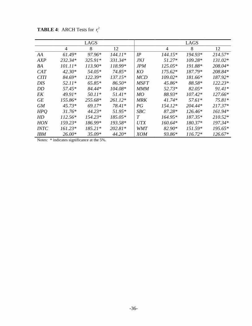
-36-

TABLE 4: ARCH Tests for 2tr

LAGS LAGS 4 8 12 4 8 12 AA 61.49* 97.96* 144.11* IP 144.15* 194.93* 214.57*AXP 232.34* 325.91* 331.34* JNJ 51.27* 109.28* 131.02*BA 101.11* 113.90* 118.99* JPM 125.05* 191.88* 208.04*CAT 42.30* 54.05* 74.85* KO 175.62* 187.79* 208.84*CITI 84.69* 122.39* 137.15* MCD 109.02* 181.66* 187.92*DIS 52.11* 65.85* 86.50* MSFT 45.86* 88.58* 122.23*DD 57.45* 84.44* 104.08* MMM 52.73* 82.05* 91.41*EK 49.91* 50.11* 51.41* MO 88.93* 107.42* 127.66*GE 155.86* 255.68* 261.12* MRK 41.74* 57.61* 75.81*GM 45.73* 69.17* 78.41* PG 154.12* 204.44* 217.37*HPQ 31.76* 44.23* 51.95* SBC 87.28* 126.46* 161.94*HD 112.56* 154.23* 185.05* T 164.95* 187.35* 210.52*HON 159.23* 186.99* 193.58* UTX 160.64* 180.37* 197.34*INTC 161.23* 185.21* 202.81* WMT 82.90* 151.59* 195.65*IBM 26.00* 35.09* 44.20* XOM 93.86* 116.72* 126.67*Notes: * indicates significance at the 5%.

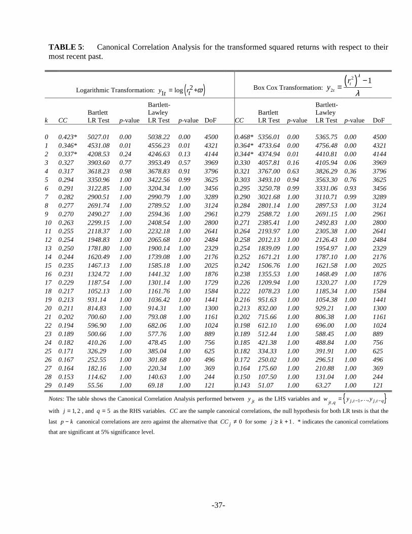
-37-

TABLE 5: Canonical Correlation Analysis for the transformed squared returns with respect to their most recent past.

Logarithmic Transformation: ( )2log1y rtt ϖ= + Box Cox Transformation:

( )22

1tt

ry

λ

λ−

=

k CC Bartlett LR Test p-value

Bartlett-Lawley LR Test p-value DoF CC

Bartlett LR Test p-value

Bartlett-Lawley LR Test p-value DoF

0 0.423* 5027.01 0.00 5038.22 0.00 4500 0.468* 5356.01 0.00 5365.75 0.00 4500 1 0.346* 4531.08 0.01 4556.23 0.01 4321 0.364* 4733.64 0.00 4756.48 0.00 4321 2 0.337* 4208.53 0.24 4246.63 0.13 4144 0.344* 4374.94 0.01 4410.81 0.00 4144 3 0.327 3903.60 0.77 3953.49 0.57 3969 0.330 4057.81 0.16 4105.94 0.06 3969 4 0.317 3618.23 0.98 3678.83 0.91 3796 0.321 3767.00 0.63 3826.29 0.36 3796 5 0.294 3350.96 1.00 3422.56 0.99 3625 0.303 3493.10 0.94 3563.30 0.76 3625 6 0.291 3122.85 1.00 3204.34 1.00 3456 0.295 3250.78 0.99 3331.06 0.93 3456 7 0.282 2900.51 1.00 2990.79 1.00 3289 0.290 3021.68 1.00 3110.71 0.99 3289 8 0.277 2691.74 1.00 2789.52 1.00 3124 0.284 2801.14 1.00 2897.53 1.00 3124 9 0.270 2490.27 1.00 2594.36 1.00 2961 0.279 2588.72 1.00 2691.15 1.00 2961 10 0.263 2299.15 1.00 2408.54 1.00 2800 0.271 2385.41 1.00 2492.83 1.00 2800 11 0.255 2118.37 1.00 2232.18 1.00 2641 0.264 2193.97 1.00 2305.38 1.00 2641 12 0.254 1948.83 1.00 2065.68 1.00 2484 0.258 2012.13 1.00 2126.43 1.00 2484 13 0.250 1781.80 1.00 1900.14 1.00 2329 0.254 1839.09 1.00 1954.97 1.00 2329 14 0.244 1620.49 1.00 1739.08 1.00 2176 0.252 1671.21 1.00 1787.10 1.00 2176 15 0.235 1467.13 1.00 1585.18 1.00 2025 0.242 1506.76 1.00 1621.58 1.00 2025 16 0.231 1324.72 1.00 1441.32 1.00 1876 0.238 1355.53 1.00 1468.49 1.00 1876 17 0.229 1187.54 1.00 1301.14 1.00 1729 0.226 1209.94 1.00 1320.27 1.00 1729 18 0.217 1052.13 1.00 1161.76 1.00 1584 0.222 1078.23 1.00 1185.34 1.00 1584 19 0.213 931.14 1.00 1036.42 1.00 1441 0.216 951.63 1.00 1054.38 1.00 1441 20 0.211 814.83 1.00 914.31 1.00 1300 0.213 832.00 1.00 929.21 1.00 1300 21 0.202 700.60 1.00 793.08 1.00 1161 0.202 715.66 1.00 806.38 1.00 1161 22 0.194 596.90 1.00 682.06 1.00 1024 0.198 612.10 1.00 696.00 1.00 1024 23 0.189 500.66 1.00 577.76 1.00 889 0.189 512.44 1.00 588.45 1.00 889 24 0.182 410.26 1.00 478.45 1.00 756 0.185 421.38 1.00 488.84 1.00 756 25 0.171 326.29 1.00 385.04 1.00 625 0.182 334.33 1.00 391.91 1.00 625 26 0.167 252.55 1.00 301.68 1.00 496 0.172 250.02 1.00 296.51 1.00 496 27 0.164 182.16 1.00 220.34 1.00 369 0.164 175.60 1.00 210.88 1.00 369 28 0.153 114.62 1.00 140.63 1.00 244 0.150 107.50 1.00 131.04 1.00 244 29 0.149 55.56 1.00 69.18 1.00 121 0.143 51.07 1.00 63.27 1.00 121

Notes: The table shows the Canonical Correlation Analysis performed between jty as the LHS variables and , 1 ,,, ,j t j t qjt q

w y y− −= …

with 1, 2j = , and 5q = as the RHS variables. CC are the sample canonical correlations, the null hypothesis for both LR tests is that the

last p k− canonical correlations are zero against the alternative that 0jCC ≠ for some 1j k≥ + . * indicates the canonical correlations

that are significant at 5% significance level.

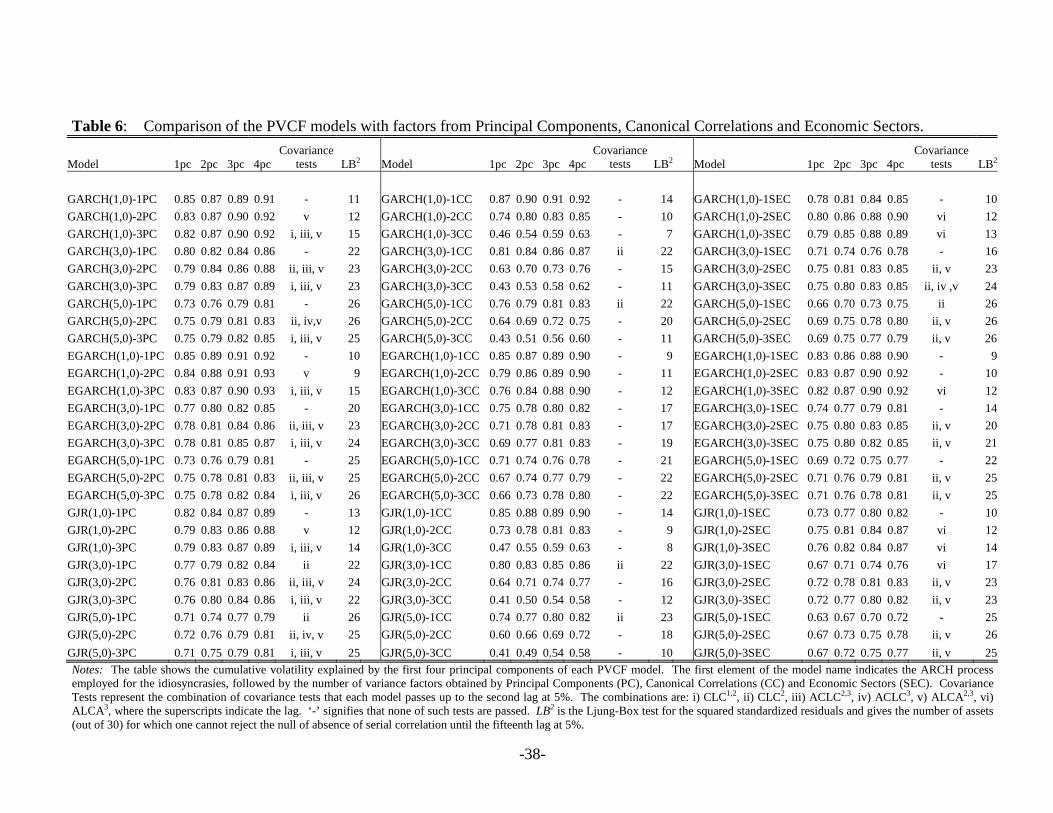
-38-

Table 6: Comparison of the PVCF models with factors from Principal Components, Canonical Correlations and Economic Sectors.

Model 1pc 2pc 3pc 4pc Covariance

tests LB2 Model 1pc 2pc 3pc 4pc

Covariance tests LB2 Model 1pc 2pc 3pc 4pc

Covariance tests LB2

GARCH(1,0)-1PC 0.85 0.87 0.89 0.91 - 11 GARCH(1,0)-1CC 0.87 0.90 0.91 0.92 - 14 GARCH(1,0)-1SEC 0.78 0.81 0.84 0.85 - 10 GARCH(1,0)-2PC 0.83 0.87 0.90 0.92 v 12 GARCH(1,0)-2CC 0.74 0.80 0.83 0.85 - 10 GARCH(1,0)-2SEC 0.80 0.86 0.88 0.90 vi 12 GARCH(1,0)-3PC 0.82 0.87 0.90 0.92 i, iii, v 15 GARCH(1,0)-3CC 0.46 0.54 0.59 0.63 - 7 GARCH(1,0)-3SEC 0.79 0.85 0.88 0.89 vi 13 GARCH(3,0)-1PC 0.80 0.82 0.84 0.86 - 22 GARCH(3,0)-1CC 0.81 0.84 0.86 0.87 ii 22 GARCH(3,0)-1SEC 0.71 0.74 0.76 0.78 - 16 GARCH(3,0)-2PC 0.79 0.84 0.86 0.88 ii, iii, v 23 GARCH(3,0)-2CC 0.63 0.70 0.73 0.76 - 15 GARCH(3,0)-2SEC 0.75 0.81 0.83 0.85 ii, v 23 GARCH(3,0)-3PC 0.79 0.83 0.87 0.89 i, iii, v 23 GARCH(3,0)-3CC 0.43 0.53 0.58 0.62 - 11 GARCH(3,0)-3SEC 0.75 0.80 0.83 0.85 ii, iv ,v 24 GARCH(5,0)-1PC 0.73 0.76 0.79 0.81 - 26 GARCH(5,0)-1CC 0.76 0.79 0.81 0.83 ii 22 GARCH(5,0)-1SEC 0.66 0.70 0.73 0.75 ii 26 GARCH(5,0)-2PC 0.75 0.79 0.81 0.83 ii, iv,v 26 GARCH(5,0)-2CC 0.64 0.69 0.72 0.75 - 20 GARCH(5,0)-2SEC 0.69 0.75 0.78 0.80 ii, v 26 GARCH(5,0)-3PC 0.75 0.79 0.82 0.85 i, iii, v 25 GARCH(5,0)-3CC 0.43 0.51 0.56 0.60 - 11 GARCH(5,0)-3SEC 0.69 0.75 0.77 0.79 ii, v 26 EGARCH(1,0)-1PC 0.85 0.89 0.91 0.92 - 10 EGARCH(1,0)-1CC 0.85 0.87 0.89 0.90 - 9 EGARCH(1,0)-1SEC 0.83 0.86 0.88 0.90 - 9 EGARCH(1,0)-2PC 0.84 0.88 0.91 0.93 v 9 EGARCH(1,0)-2CC 0.79 0.86 0.89 0.90 - 11 EGARCH(1,0)-2SEC 0.83 0.87 0.90 0.92 - 10 EGARCH(1,0)-3PC 0.83 0.87 0.90 0.93 i, iii, v 15 EGARCH(1,0)-3CC 0.76 0.84 0.88 0.90 - 12 EGARCH(1,0)-3SEC 0.82 0.87 0.90 0.92 vi 12 EGARCH(3,0)-1PC 0.77 0.80 0.82 0.85 - 20 EGARCH(3,0)-1CC 0.75 0.78 0.80 0.82 - 17 EGARCH(3,0)-1SEC 0.74 0.77 0.79 0.81 - 14 EGARCH(3,0)-2PC 0.78 0.81 0.84 0.86 ii, iii, v 23 EGARCH(3,0)-2CC 0.71 0.78 0.81 0.83 - 17 EGARCH(3,0)-2SEC 0.75 0.80 0.83 0.85 ii, v 20 EGARCH(3,0)-3PC 0.78 0.81 0.85 0.87 i, iii, v 24 EGARCH(3,0)-3CC 0.69 0.77 0.81 0.83 - 19 EGARCH(3,0)-3SEC 0.75 0.80 0.82 0.85 ii, v 21 EGARCH(5,0)-1PC 0.73 0.76 0.79 0.81 - 25 EGARCH(5,0)-1CC 0.71 0.74 0.76 0.78 - 21 EGARCH(5,0)-1SEC 0.69 0.72 0.75 0.77 - 22 EGARCH(5,0)-2PC 0.75 0.78 0.81 0.83 ii, iii, v 25 EGARCH(5,0)-2CC 0.67 0.74 0.77 0.79 - 22 EGARCH(5,0)-2SEC 0.71 0.76 0.79 0.81 ii, v 25 EGARCH(5,0)-3PC 0.75 0.78 0.82 0.84 i, iii, v 26 EGARCH(5,0)-3CC 0.66 0.73 0.78 0.80 - 22 EGARCH(5,0)-3SEC 0.71 0.76 0.78 0.81 ii, v 25 GJR(1,0)-1PC 0.82 0.84 0.87 0.89 - 13 GJR(1,0)-1CC 0.85 0.88 0.89 0.90 - 14 GJR(1,0)-1SEC 0.73 0.77 0.80 0.82 - 10 GJR(1,0)-2PC 0.79 0.83 0.86 0.88 v 12 GJR(1,0)-2CC 0.73 0.78 0.81 0.83 - 9 GJR(1,0)-2SEC 0.75 0.81 0.84 0.87 vi 12 GJR(1,0)-3PC 0.79 0.83 0.87 0.89 i, iii, v 14 GJR(1,0)-3CC 0.47 0.55 0.59 0.63 - 8 GJR(1,0)-3SEC 0.76 0.82 0.84 0.87 vi 14 GJR(3,0)-1PC 0.77 0.79 0.82 0.84 ii 22 GJR(3,0)-1CC 0.80 0.83 0.85 0.86 ii 22 GJR(3,0)-1SEC 0.67 0.71 0.74 0.76 vi 17 GJR(3,0)-2PC 0.76 0.81 0.83 0.86 ii, iii, v 24 GJR(3,0)-2CC 0.64 0.71 0.74 0.77 - 16 GJR(3,0)-2SEC 0.72 0.78 0.81 0.83 ii, v 23 GJR(3,0)-3PC 0.76 0.80 0.84 0.86 i, iii, v 22 GJR(3,0)-3CC 0.41 0.50 0.54 0.58 - 12 GJR(3,0)-3SEC 0.72 0.77 0.80 0.82 ii, v 23 GJR(5,0)-1PC 0.71 0.74 0.77 0.79 ii 26 GJR(5,0)-1CC 0.74 0.77 0.80 0.82 ii 23 GJR(5,0)-1SEC 0.63 0.67 0.70 0.72 - 25 GJR(5,0)-2PC 0.72 0.76 0.79 0.81 ii, iv, v 25 GJR(5,0)-2CC 0.60 0.66 0.69 0.72 - 18 GJR(5,0)-2SEC 0.67 0.73 0.75 0.78 ii, v 26 GJR(5,0)-3PC 0.71 0.75 0.79 0.81 i, iii, v 25 GJR(5,0)-3CC 0.41 0.49 0.54 0.58 - 10 GJR(5,0)-3SEC 0.67 0.72 0.75 0.77 ii, v 25 Notes: The table shows the cumulative volatility explained by the first four principal components of each PVCF model. The first element of the model name indicates the ARCH process employed for the idiosyncrasies, followed by the number of variance factors obtained by Principal Components (PC), Canonical Correlations (CC) and Economic Sectors (SEC). Covariance Tests represent the combination of covariance tests that each model passes up to the second lag at 5%. The combinations are: i) CLC1,2, ii) CLC2, iii) ACLC2,3, iv) ACLC3, v) ALCA2,3, vi) ALCA3, where the superscripts indicate the lag. ‘-’ signifies that none of such tests are passed. LB2 is the Ljung-Box test for the squared standardized residuals and gives the number of assets (out of 30) for which one cannot reject the null of absence of serial correlation until the fifteenth lag at 5%.

-39-

Table 7: Comparison of the PVCF models with Market factors. Model 1pc 2pc 3pc 4pc

Covariance tests LB2 Model 1pc 2pc 3pc 4pc

Covariance tests LB2 Model 1pc 2pc 3pc 4pc Covariance

tests LB2 GARCH(1,0)-NQ 0.85 0.88 0.90 0.91 - 7 EGARCH(1,0)-NQ 0.86 0.88 0.90 0.92 - 8 GJR(1,0)-NQ 0.82 0.85 0.88 0.90 - 7 GARCH(1,0)-VX 0.79 0.81 0.84 0.86 - 9 EGARCH(1,0)-VX 0.83 0.85 0.88 0.89 - 8 GJR(1,0)-VX 0.76 0.79 0.82 0.84 - 8 GARCH(1,0)-DJ 0.84 0.87 0.89 0.90 - 12 EGARCH(1,0)-DJ 0.84 0.88 0.90 0.91 - 10 GJR(1,0)-DJ 0.81 0.84 0.86 0.88 - 13 GARCH(1,0)-SP 0.83 0.86 0.88 0.90 - 10 EGARCH(1,0)-SP 0.84 0.87 0.89 0.91 - 7 GJR(1,0)-SP 0.80 0.83 0.85 0.88 - 10 GARCH(1,0)-NQVX 0.80 0.85 0.88 0.90 - 12 EGARCH(1,0)-NQVX 0.83 0.87 0.89 0.91 - 8 GJR(1,0)-NQVX 0.78 0.83 0.86 0.88 - 11 GARCH(1,0)-NQDJ 0.82 0.88 0.91 0.92 - 13 EGARCH(1,0)-NQDJ 0.83 0.88 0.90 0.92 - 10 GJR(1,0)-NQDJ 0.79 0.85 0.87 0.90 - 13 GARCH(1,0)-DJVX 0.81 0.83 0.86 0.87 - 11 EGARCH(1,0)-DJVX 0.84 0.86 0.88 0.90 - 8 GJR(1,0)-DJVX 0.77 0.80 0.83 0.85 - 10 GARCH(1,0)-DJSP 0.82 0.85 0.87 0.89 - 12 EGARCH(1,0)-DJSP 0.83 0.86 0.88 0.90 - 9 GJR(1,0)-DJSP 0.78 0.82 0.85 0.87 - 13 GARCH(1,0)-SPNQ 0.81 0.87 0.90 0.92 - 12 EGARCH(1,0)-SPNQ 0.83 0.88 0.90 0.92 - 9 GJR(1,0)-SPNQ 0.78 0.84 0.87 0.89 - 13 GARCH(1,0)-SPVX 0.80 0.83 0.86 0.88 - 10 EGARCH(1,0)-SPVX 0.83 0.86 0.88 0.90 - 7 GJR(1,0)-SPVX 0.77 0.81 0.83 0.85 - 10 GARCH(1,0)-VXSP 0.78 0.84 0.87 0.89 - 11 EGARCH(1,0)-VXSP 0.81 0.86 0.89 0.91 - 8 GJR(1,0)-VXSP 0.76 0.82 0.85 0.87 - 11 GARCH(1,0)-NQVXDJ 0.79 0.85 0.88 0.90 - 11 EGARCH(1,0)-NQVXDJ 0.82 0.87 0.89 0.91 - 9 GJR(1,0)-NQVXDJ 0.76 0.83 0.85 0.88 - 12 GARCH(1,0)-DJSPNQ 0.81 0.87 0.89 0.91 - 14 EGARCH(1,0)-DJSPNQ 0.82 0.87 0.90 0.91 - 11 GJR(1,0)-DJSPNQ 0.77 0.83 0.86 0.88 - 14 GARCH(1,0)-DJVXSP 0.77 0.82 0.84 0.86 - 10 EGARCH(1,0)-DJVXSP 0.81 0.85 0.88 0.89 - 8 GJR(1,0)-DJVXSP 0.75 0.80 0.82 0.84 - 10 GARCH(3,0)-NQ 0.80 0.83 0.85 0.87 - 21 EGARCH(3,0)-NQ 0.77 0.81 0.83 0.85 - 20 GJR(3,0)-NQ 0.77 0.80 0.83 0.84 - 21 GARCH(3,0)-VX 0.72 0.75 0.78 0.80 - 18 EGARCH(3,0)-VX 0.74 0.77 0.79 0.81 - 13 GJR(3,0)-VX 0.70 0.73 0.76 0.78 - 19 GARCH(3,0)-DJ 0.78 0.80 0.82 0.84 - 20 EGARCH(3,0)-DJ 0.75 0.78 0.81 0.83 - 20 GJR(3,0)-DJ 0.74 0.77 0.79 0.81 - 19 GARCH(3,0)-SP 0.78 0.80 0.83 0.84 - 23 EGARCH(3,0)-SP 0.75 0.78 0.81 0.83 - 20 GJR(3,0)-SP 0.75 0.78 0.80 0.82 - 22 GARCH(3,0)-NQVX 0.76 0.82 0.84 0.86 - 23 EGARCH(3,0)-NQVX 0.76 0.81 0.83 0.86 - 23 GJR(3,0)-NQVX 0.74 0.79 0.82 0.85 - 23 GARCH(3,0)-NQDJ 0.79 0.84 0.87 0.89 ii, vi 23 EGARCH(3,0)-NQDJ 0.77 0.82 0.84 0.86 ii, vi 25 GJR(3,0)-NQDJ 0.76 0.82 0.84 0.86 ii, vi 24 GARCH(3,0)-DJVX 0.75 0.78 0.80 0.82 - 21 EGARCH(3,0)-DJVX 0.75 0.78 0.81 0.83 - 18 GJR(3,0)-DJVX 0.72 0.75 0.78 0.80 - 21 GARCH(3,0)-DJSP 0.76 0.79 0.82 0.84 - 23 EGARCH(3,0)-DJSP 0.74 0.77 0.80 0.82 - 20 GJR(3,0)-DJSP 0.73 0.76 0.79 0.81 - 23 GARCH(3,0)-SPNQ 0.78 0.83 0.86 0.88 ii, vi 23 EGARCH(3,0)-SPNQ 0.77 0.81 0.84 0.86 ii, vi 24 GJR(3,0)-SPNQ 0.75 0.81 0.84 0.86 ii, vi 23 GARCH(3,0)-SPVX 0.75 0.78 0.81 0.83 - 22 EGARCH(3,0)-SPVX 0.74 0.78 0.81 0.83 - 18 GJR(3,0)-SPVX 0.72 0.76 0.78 0.81 - 21 GARCH(3,0)-VXSP 0.75 0.81 0.84 0.86 - 24 EGARCH(3,0)-VXSP 0.75 0.79 0.83 0.85 - 24 GJR(3,0)-VXSP 0.73 0.79 0.82 0.84 - 24 GARCH(3,0)-NQVXDJ 0.75 0.81 0.84 0.86 - 24 EGARCH(3,0)-NQVXDJ 0.75 0.80 0.83 0.85 - 22 GJR(3,0)-NQVXDJ 0.73 0.79 0.82 0.84 - 24 GARCH(3,0)-DJSPNQ 0.77 0.83 0.86 0.88 ii, vi 24 EGARCH(3,0)-DJSPNQ 0.76 0.80 0.83 0.85 ii, vi 25 GJR(3,0)-DJSPNQ 0.75 0.80 0.83 0.85 ii, vi 24 GARCH(3,0)-DJVXSP 0.72 0.77 0.79 0.82 - 22 EGARCH(3,0)-DJVXSP 0.73 0.77 0.80 0.82 - 18 GJR(3,0)-DJVXSP 0.70 0.75 0.78 0.80 - 23 Notes: The table shows the cumulative volatility explained by the first four principal components of each PVCF-MKT model. The first element of the model name indicates the ARCH process employed for the idiosyncrasies, followed by the variance factors which are the volatilities of the Dow Jones (DJ), NASDAQ (NQ), S&P500 (SP) indices or the VIX (VX). Covariance Tests represent the combination of covariance tests that each model passes up to the second lag at 5%. The combinations are: i) CLC1,2, ii) CLC2, iii) ACLC2,3, iv) ACLC3, v) ALCA2,3, vi) ALCA3, where the superscripts indicate the lag. ‘-’ signifies that none of such tests are passed. LB2 is the Ljung-Box test for the squared standardized residuals and gives the number of assets (out of 30) for which one cannot reject the null of absence of serial correlation until the fifteenth lag at 5%.

-40-

Table 7: Continued

Model 1pc 2pc 3pc 4pc Covariance

tests LB2 Model 1pc 2pc 3pc 4pc

Covariance tests LB2

Model 1pc 2pc 3pc 4pcCovariance

tests LB2 GARCH(5,0)-NQ 0.76 0.80 0.82 0.84 - 25 EGARCH(5,0)-NQ 0.74 0.77 0.80 0.82 ii 22 GJR(5,0)-NQ 0.72 0.75 0.78 0.80 - 23 GARCH(5,0)-VX 0.67 0.71 0.73 0.76 - 24 EGARCH(5,0)-VX 0.70 0.73 0.76 0.78 - 21 GJR(5,0)-VX 0.66 0.69 0.72 0.75 - 24 GARCH(5,0)-DJ 0.73 0.76 0.78 0.80 - 25 EGARCH(5,0)-DJ 0.71 0.74 0.77 0.79 - 24 GJR(5,0)-DJ 0.71 0.74 0.76 0.78 - 25 GARCH(5,0)-SP 0.74 0.77 0.79 0.81 - 26 EGARCH(5,0)-SP 0.71 0.74 0.77 0.79 - 24 GJR(5,0)-SP 0.71 0.74 0.76 0.78 - 26 GARCH(5,0)-NQVX 0.71 0.76 0.79 0.81 - 23 EGARCH(5,0)-NQVX 0.74 0.78 0.81 0.83 - 23 GJR(5,0)-NQVX 0.71 0.75 0.78 0.80 - 24 GARCH(5,0)-NQDJ 0.75 0.81 0.83 0.85 ii 26 EGARCH(5,0)-NQDJ 0.74 0.78 0.81 0.83 ii, vi 25 GJR(5,0)-NQDJ 0.73 0.78 0.81 0.83 ii, vi 26 GARCH(5,0)-DJVX 0.70 0.74 0.76 0.78 - 24 EGARCH(5,0)-DJVX 0.72 0.75 0.77 0.79 - 22 GJR(5,0)-DJVX 0.68 0.72 0.74 0.76 - 24 GARCH(5,0)-DJSP 0.71 0.75 0.77 0.79 - 26 EGARCH(5,0)-DJSP 0.70 0.74 0.76 0.78 - 24 GJR(5,0)-DJSP 0.69 0.72 0.75 0.77 - 25 GARCH(5,0)-SPNQ 0.76 0.81 0.84 0.86 ii 27 EGARCH(5,0)-SPNQ 0.73 0.78 0.80 0.83 ii, vi 25 GJR(5,0)-SPNQ 0.73 0.78 0.81 0.83 ii, vi 27 GARCH(5,0)-SPVX 0.70 0.74 0.76 0.79 - 25 EGARCH(5,0)-SPVX 0.71 0.75 0.78 0.80 - 23 GJR(5,0)-SPVX 0.69 0.73 0.75 0.78 - 25 GARCH(5,0)-VXSP 0.71 0.77 0.80 0.82 - 25 EGARCH(5,0)-VXSP 0.72 0.77 0.80 0.82 - 25 GJR(5,0)-VXSP 0.69 0.74 0.77 0.80 - 25 GARCH(5,0)-NQVXDJ 0.73 0.79 0.82 0.84 - 25 EGARCH(5,0)-NQVXDJ 0.72 0.77 0.80 0.82 - 24 GJR(5,0)-NQVXDJ 0.71 0.77 0.80 0.82 - 25 GARCH(5,0)-DJSPNQ 0.72 0.78 0.81 0.83 ii 26 EGARCH(5,0)-DJSPNQ 0.72 0.77 0.80 0.82 ii, vi 24 GJR(5,0)-DJSPNQ 0.70 0.76 0.79 0.81 ii, vi 27 GARCH(5,0)-DJVXSP 0.68 0.72 0.75 0.77 - 24 EGARCH(5,0)-DJVXSP 0.70 0.74 0.77 0.79 - 24 GJR(5,0)-DJVXSP 0.66 0.70 0.73 0.75 - 25 Notes: The table shows the cumulative volatility explained by the first four principal components of each PVCF-MKT model. The first element of the model name indicates the ARCH process employed for the idiosyncrasies, followed by the variance factors which are the volatilities of the Dow Jones (DJ), NASDAQ (NQ), S&P500 (SP) indices or the VIX (VX). Covariance Tests represent the combination of covariance tests that each model passes up to the second lag at 5%. The combinations are: i) CLC1,2, ii) CLC2, iii) ACLC2,3, iv) ACLC3, v) ALCA2,3, vi) ALCA3, where the superscripts indicate the lag. ‘-’ signifies that none of such tests are passed. LB2 is the Ljung-Box test for the squared standardized residuals and gives the number of assets (out of 30) for which one cannot reject the null of absence of serial correlation until the fifteenth lag at 5%.

-41-

TABLE 8: Estimation results for the best PVCF-MKT model: the GJR(5,0)-SPNQ. SP500 NASDAQ SP500 NASDAQ SP500 NASDAQ Vol. Fact. Vol. Fact. LB2 Vol. Fact. Vol. Fact. LB2 Vol. Fact. Vol. Fact. LB2

AA -0.1656 0.7615 OK HD 0.0930 0.6993 OK MMM 0.7398 0.1102 OK (0.3310) (0.1280) (0.3435) (0.1194) 0.2935 0.0657 AXP 1.7893 0.2527 OK HON 1.0339 0.4819 OK MO 2.3727 0.0095 OK (0.5287) (0.1056) (0.5689) (0.1341) (0.5798) (0.1210) BA 2.1722 0.0767 OK HPQ 0.7139 1.1210 OK MRK 1.0406 -0.0174 OK (0.6359) (0.1248) (0.8526) (0.2405) (0.2842) (0.0676) CAT 1.7831 0.0244 OK IBM 0.7057 0.4451 OK MSFT -0.4250 0.7604 OK (0.5204) (0.1006) (0.6139) (0.1746) (0.3966) (0.1854) CITI 1.6516 -0.0683 OK INTC -0.3426 1.2228 OK PG 0.9061 0.1522 OK (0.5129) (0.1227) (0.5456) (0.2256) (0.3102) (0.0958) DD 1.8863 0.1034 OK IP 1.5059 0.2309 OK SBC 0.8445 0.2906 9 (0.4020) (0.1066) (0.4258) (0.1095) (0.3038) (0.1063) DIS 0.8323 0.4647 OK JNJ 0.4354 -0.0305 6 T 1.0560 0.5777 OK (0.4876) (0.1639) (0.2344) (0.0435) (0.5362) (0.1368) EK 0.8932 0.0275 OK JPM 1.0346 0.5103 OK UTX 0.9500 0.1792 OK (0.4669) (0.0950) (0.5148) (0.1536) (0.2490) (0.0617) GE 1.2857 0.1429 OK KO 0.9148 0.1317 OK WMT 0.5756 0.4221 10 (0.2964) (0.0680) (0.2778) (0.0750) (0.3195) (0.1088) GM 0.1886 0.3131 OK MCD 0.7008 0.1933 OK XOM 1.2691 -0.0435 OK

(0.2678) (0.0811) (0.2832) (0.0699) (0.2027) (0.0482) Covariance Tests

LC1 p-value CLC1 p-value CLC2 p-value CLC3 p-value CLC4 p-value CLC5 p-value 6013.85 0 10.68 0 3.83 0.05 2.26 0.13 2.36 0.12 4.98 0.03

ALC1 p-value ACLC2 p-value ACLC3 p-value AALC2 p-value AALC3 p-value 1071.67 0 11.21 0 12.02 0.01 7.71 0.02 7.87 0.05 Notes: The estimated PVCF model is a GJR(5,0) for the short-run volatility component (whose estimates are not reported) and two market volatility factors, given by the estimated volatility of the S&P500, and the NASDAQ. Robust standard errors (as in Bollerslev and Wooldridge, 1992) are in parentheses.

2LB represents the Ljung-Box test for the absence of serial correlation in the standardized squared residuals up to 15 lags. For each asset, the first lag at which one rejects the null at 5% is reported. Alternatively, an OK indicates that such lag is not less than 15. The superscripts in the covariance tests indicate the number of lags used.

-42-

TABLE 9: Estimation results for the best PVCF-PC model: the EGARCH(5,0)-3PC Model. First PC Second PC Third PC First PC Second PC Third PC First PC Second PC Third PC Vol. Fact. Vol. Fact. Vol. Fact. LB2 Vol. Fact. Vol. Fact. Vol. Fact. LB2 Vol. Fact. Vol. Fact. Vol. Fact. LB2

AA 0.2180 0.1929 0.5636 OK HD 0.2357 0.3438 0.3587 OK MMM 0.5240 0.0482 0.3642 OK (0.0872) (0.1022) (0.1052) (0.0991) (0.1032) (0.0917) (0.0903) (0.1004) (0.1052) AXP 0.4552 0.3304 0.2053 OK HON 0.5080 0.1412 0.4245 OK MO 0.5338 0.4370 -0.0567 OK (0.1095) (0.0875) (0.0999) (0.1424) (0.1165) (0.1086) (0.1097) (0.1221) (0.1979) BA 0.6942 0.1663 0.0988 OK HPQ 0.2753 0.5444 0.1151 OK MRK 0.1570 -0.0249 0.4425 OK (0.1110) (0.1108) (0.1320) (0.0858) (0.0822) (0.0941) (0.0926) (0.1022) (0.1112) CAT 0.3840 -0.0163 0.3278 OK IBM 0.1786 0.3377 0.3335 OK MSFT 0.1263 0.4933 0.1454 OK (0.0939) (0.0995) (0.0911) (0.1114) (0.1296) (0.1449) (0.0804) (0.1115) (0.0968) CITI 0.4071 -0.0705 0.2064 OK INTC 0.1722 0.3146 0.3491 OK PG 0.4598 0.1604 0.2648 OK (0.0998) (0.0976) (0.1080) (0.0871) (0.1137) (0.0940) (0.1067) (0.1138) (0.0983) DD 0.5460 -0.0191 0.4586 OK IP 0.4591 0.2069 0.3828 OK SBC 0.5251 0.3473 0.1881 6 (0.0878) (0.0884) (0.1148) (0.0793) (0.0960) (0.1181) (0.0812) (0.0988) (0.1011) DIS 0.4595 0.2493 0.2816 OK JNJ 0.0737 -0.0459 0.3686 5 T 0.6091 0.2280 0.4422 OK (0.1018) (0.1334) (0.1021) (0.0922) (0.0913) (0.0970) (0.1315) (0.1157) (0.1526) EK 0.3449 -0.0255 0.2280 OK JPM 0.3956 0.1824 0.3990 OK UTX 0.4418 0.0628 0.5316 OK (0.1471) (0.1294) (0.1965) (0.0940) (0.1120) (0.1002) (0.0835) (0.0868) (0.0863) GE 0.7621 0.2861 0.0232 OK KO 0.3427 0.2273 0.2847 OK WMT 0.2353 0.3094 0.3959 10 (0.0739) (0.0839) (0.0897) (0.0876) (0.1136) (0.1200) (0.0772) (0.0939) (0.0966) GM 0.1544 0.0280 0.4101 OK MCD 0.2409 0.1027 0.5447 5 XOM 0.5169 0.1040 0.2749 OK

(0.0853) (0.0967) (0.0833) (0.1259) (0.1129) (0.0943) (0.0959) (0.1012) (0.1014)

Covariance Tests

LC1 p-value CLC1 p-value CLC2 p-value CLC3 p-value CLC4 p-value CLC5 p-value

5722.17 0 1.97 0.16 0.17 0.68 0.01 0.93 0.01 0.9 1.52 0.22

ALC1 p-value ACLC2 p-value ACLC3 p-value AALC2 p-value AALC3 p-value 1073 0 2.23 0.33 2.26 0.52 1.66 0.43 2.12 0.55

Notes: The estimated PVCF model is an EGARCH(5,0) for the short-run volatility component (not reported) and three variance factors, represented by the estimated conditional volatilities of the three largest principal components of the returns. The variance factors are in logarithms because EGARCH models the log of the conditional variance. Robust standard errors (as in Bollerslev and Wooldridge, 1992) are in parentheses. 2LB represents the Ljung-Box test for the absence of serial correlation in the standardized squared residuals up to 15 lags. For each asset, the first lag at which one rejects the null at 5% is reported. Alternatively, an OK indicates that such lag is not less than 15. The superscripts in the covariance tests indicate the number of lags used.

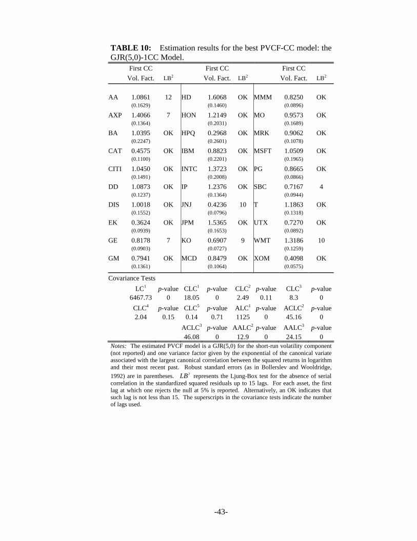
-43-

TABLE 10: Estimation results for the best PVCF-CC model: the GJR(5,0)-1CC Model.

First CC First CC First CC Vol. Fact. LB2 Vol. Fact. LB2 Vol. Fact. LB2

AA 1.0861 12 HD 1.6068 OK MMM 0.8250 OK (0.1629) (0.1460) (0.0896) AXP 1.4066 7 HON 1.2149 OK MO 0.9573 OK (0.1364) (0.2031) (0.1689) BA 1.0395 OK HPQ 0.2968 OK MRK 0.9062 OK (0.2247) (0.2601) (0.1078) CAT 0.4575 OK IBM 0.8823 OK MSFT 1.0509 OK (0.1100) (0.2201) (0.1965) CITI 1.0450 OK INTC 1.3723 OK PG 0.8665 OK (0.1491) (0.2008) (0.0866) DD 1.0873 OK IP 1.2376 OK SBC 0.7167 4 (0.1237) (0.1364) (0.0944) DIS 1.0018 OK JNJ 0.4236 10 T 1.1863 OK (0.1552) (0.0796) (0.1318) EK 0.3624 OK JPM 1.5365 OK UTX 0.7270 OK (0.0939) (0.1653) (0.0892) GE 0.8178 7 KO 0.6907 9 WMT 1.3186 10 (0.0903) (0.0727) (0.1259) GM 0.7941 OK MCD 0.8479 OK XOM 0.4098 OK

(0.1361) (0.1064) (0.0575) Covariance Tests LC1 p-value CLC1 p-value CLC2 p-value CLC3 p-value 6467.73 0 18.05 0 2.49 0.11 8.3 0 CLC4 p-value CLC5 p-value ALC1 p-value ACLC2 p-value 2.04 0.15 0.14 0.71 1125 0 45.16 0 ACLC3 p-value AALC2 p-value AALC3 p-value 46.08 0 12.9 0 24.15 0 Notes: The estimated PVCF model is a GJR(5,0) for the short-run volatility component (not reported) and one variance factor given by the exponential of the canonical variate associated with the largest canonical correlation between the squared returns in logarithm and their most recent past. Robust standard errors (as in Bollerslev and Wooldridge, 1992) are in parentheses. 2LB represents the Ljung-Box test for the absence of serial correlation in the standardized squared residuals up to 15 lags. For each asset, the first lag at which one rejects the null at 5% is reported. Alternatively, an OK indicates that such lag is not less than 15. The superscripts in the covariance tests indicate the number of lags used.

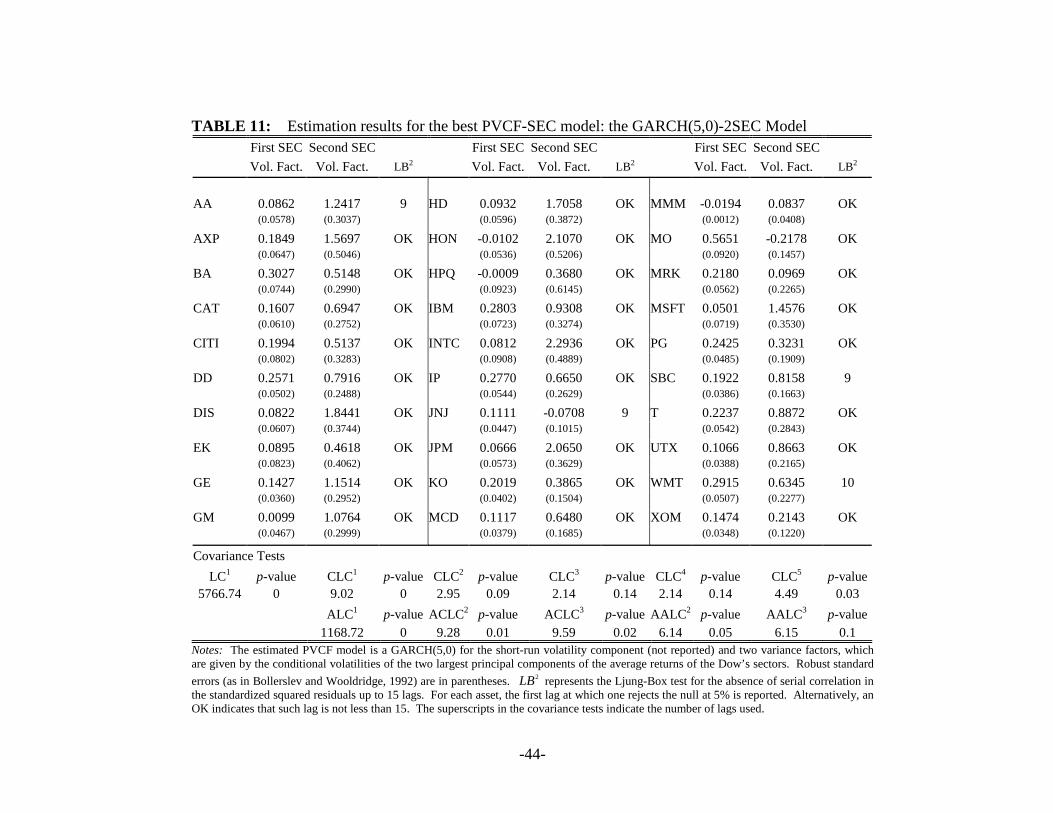
-44-

TABLE 11: Estimation results for the best PVCF-SEC model: the GARCH(5,0)-2SEC Model First SEC Second SEC First SEC Second SEC First SEC Second SEC Vol. Fact. Vol. Fact. LB2 Vol. Fact. Vol. Fact. LB2 Vol. Fact. Vol. Fact. LB2

AA 0.0862 1.2417 9 HD 0.0932 1.7058 OK MMM -0.0194 0.0837 OK (0.0578) (0.3037) (0.0596) (0.3872) (0.0012) (0.0408) AXP 0.1849 1.5697 OK HON -0.0102 2.1070 OK MO 0.5651 -0.2178 OK (0.0647) (0.5046) (0.0536) (0.5206) (0.0920) (0.1457) BA 0.3027 0.5148 OK HPQ -0.0009 0.3680 OK MRK 0.2180 0.0969 OK (0.0744) (0.2990) (0.0923) (0.6145) (0.0562) (0.2265) CAT 0.1607 0.6947 OK IBM 0.2803 0.9308 OK MSFT 0.0501 1.4576 OK (0.0610) (0.2752) (0.0723) (0.3274) (0.0719) (0.3530) CITI 0.1994 0.5137 OK INTC 0.0812 2.2936 OK PG 0.2425 0.3231 OK (0.0802) (0.3283) (0.0908) (0.4889) (0.0485) (0.1909) DD 0.2571 0.7916 OK IP 0.2770 0.6650 OK SBC 0.1922 0.8158 9 (0.0502) (0.2488) (0.0544) (0.2629) (0.0386) (0.1663) DIS 0.0822 1.8441 OK JNJ 0.1111 -0.0708 9 T 0.2237 0.8872 OK (0.0607) (0.3744) (0.0447) (0.1015) (0.0542) (0.2843) EK 0.0895 0.4618 OK JPM 0.0666 2.0650 OK UTX 0.1066 0.8663 OK (0.0823) (0.4062) (0.0573) (0.3629) (0.0388) (0.2165) GE 0.1427 1.1514 OK KO 0.2019 0.3865 OK WMT 0.2915 0.6345 10 (0.0360) (0.2952) (0.0402) (0.1504) (0.0507) (0.2277) GM 0.0099 1.0764 OK MCD 0.1117 0.6480 OK XOM 0.1474 0.2143 OK (0.0467) (0.2999) (0.0379) (0.1685) (0.0348) (0.1220) Covariance Tests

LC1 p-value CLC1 p-value CLC2 p-value CLC3 p-value CLC4 p-value CLC5 p-value5766.74 0 9.02 0 2.95 0.09 2.14 0.14 2.14 0.14 4.49 0.03

ALC1 p-value ACLC2 p-value ACLC3 p-value AALC2 p-value AALC3 p-value 1168.72 0 9.28 0.01 9.59 0.02 6.14 0.05 6.15 0.1 Notes: The estimated PVCF model is a GARCH(5,0) for the short-run volatility component (not reported) and two variance factors, which are given by the conditional volatilities of the two largest principal components of the average returns of the Dow’s sectors. Robust standard errors (as in Bollerslev and Wooldridge, 1992) are in parentheses. 2LB represents the Ljung-Box test for the absence of serial correlation in the standardized squared residuals up to 15 lags. For each asset, the first lag at which one rejects the null at 5% is reported. Alternatively, an OK indicates that such lag is not less than 15. The superscripts in the covariance tests indicate the number of lags used.

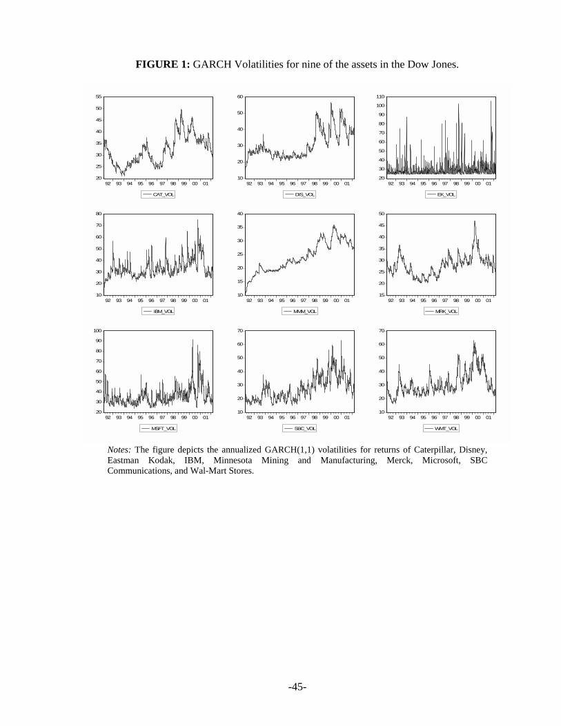
-45-

FIGURE 1: GARCH Volatilities for nine of the assets in the Dow Jones.

20

25

30

35

40

45

50

55

92 93 94 95 96 97 98 99 00 01

CAT_VOL

10

20

30

40

50

60

92 93 94 95 96 97 98 99 00 01

DIS_VOL

20

30

40

50

60

70

80

90

100

110

92 93 94 95 96 97 98 99 00 01

EK_VOL

10

20

30

40

50

60

70

80

92 93 94 95 96 97 98 99 00 01

IBM_VOL

10

15

20

25

30

35

40

92 93 94 95 96 97 98 99 00 01

MMM_VOL

15

20

25

30

35

40

45

50

92 93 94 95 96 97 98 99 00 01

MRK_VOL

20

30

40

50

60

70

80

90

100

92 93 94 95 96 97 98 99 00 01

MSFT_VOL

10

20

30

40

50

60

70

92 93 94 95 96 97 98 99 00 01

SBC_VOL

10

20

30

40

50

60

70

92 93 94 95 96 97 98 99 00 01

WMT_VOL

Notes: The figure depicts the annualized GARCH(1,1) volatilities for returns of Caterpillar, Disney, Eastman Kodak, IBM, Minnesota Mining and Manufacturing, Merck, Microsoft, SBC Communications, and Wal-Mart Stores.

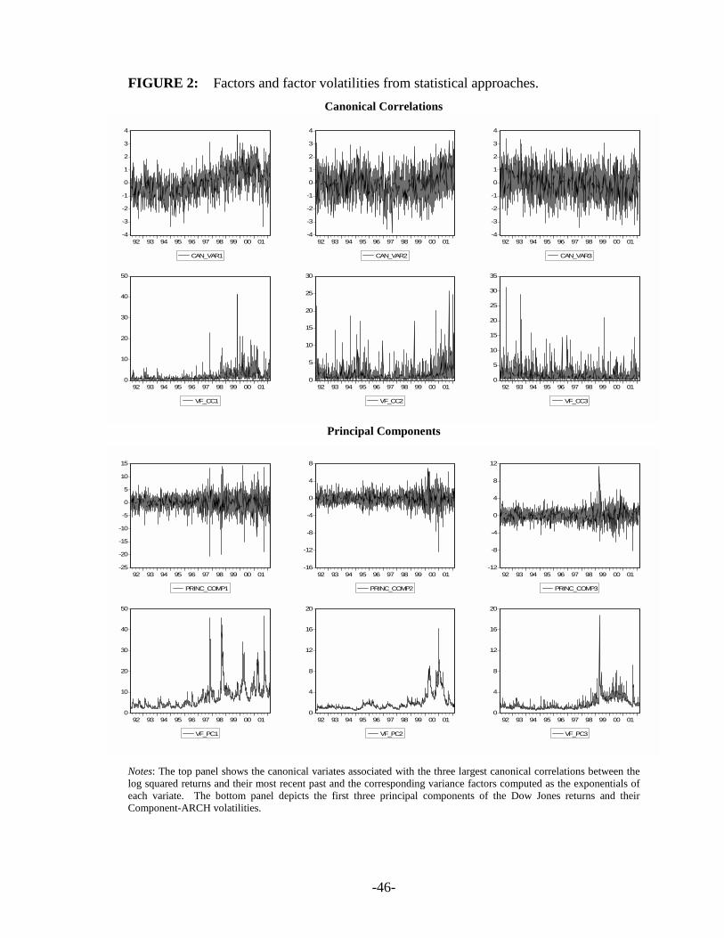
-46-

FIGURE 2: Factors and factor volatilities from statistical approaches.

Canonical Correlations

-4

-3

-2

-1

0

1

2

3

4

92 93 94 95 96 97 98 99 00 01

CAN_VAR1

-4

-3

-2

-1

0

1

2

3

4

92 93 94 95 96 97 98 99 00 01

CAN_VAR2

-4

-3

-2

-1

0

1

2

3

4

92 93 94 95 96 97 98 99 00 01

CAN_VAR3

0

10

20

30

40

50

92 93 94 95 96 97 98 99 00 01

VF_CC1

0

5

10

15

20

25

30

92 93 94 95 96 97 98 99 00 01

VF_CC2

0

5

10

15

20

25

30

35

92 93 94 95 96 97 98 99 00 01

VF_CC3

Principal Components

-25

-20

-15

-10

-5

0

5

10

15

92 93 94 95 96 97 98 99 00 01

PRINC_COMP1

-16

-12

-8

-4

0

4

8

92 93 94 95 96 97 98 99 00 01

PRINC_COMP2

-12

-8

-4

0

4

8

12

92 93 94 95 96 97 98 99 00 01

PRINC_COMP3

0

10

20

30

40

50

92 93 94 95 96 97 98 99 00 01

VF_PC1

0

4

8

12

16

20

92 93 94 95 96 97 98 99 00 01

VF_PC2

0

4

8

12

16

20

92 93 94 95 96 97 98 99 00 01

VF_PC3

Notes: The top panel shows the canonical variates associated with the three largest canonical correlations between the log squared returns and their most recent past and the corresponding variance factors computed as the exponentials of each variate. The bottom panel depicts the first three principal components of the Dow Jones returns and their Component-ARCH volatilities.

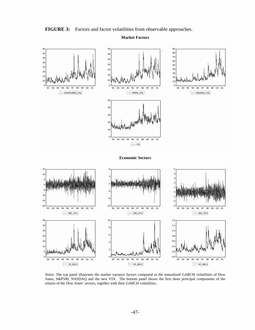
-47-

FIGURE 3: Factors and factor volatilities from observable approaches.

Market Factors

5

10

15

20

25

30

35

40

45

92 93 94 95 96 97 98 99 00 01

DOWJONES_VOL

5

10

15

20

25

30

35

40

92 93 94 95 96 97 98 99 00 01

SP500_VOL

0

10

20

30

40

50

60

70

80

90

92 93 94 95 96 97 98 99 00 01

NASDAQ_VOL

0

10

20

30

40

50

92 93 94 95 96 97 98 99 00 01

VIX

Economic Sectors

-20

-15

-10

-5

0

5

10

15

92 93 94 95 96 97 98 99 00 01

SEC_PC1

-12

-8

-4

0

4

8

92 93 94 95 96 97 98 99 00 01

SEC_PC2

-3

-2

-1

0

1

2

3

4

5

92 93 94 95 96 97 98 99 00 01

SEC_PC3

0

5

10

15

20

25

30

35

92 93 94 95 96 97 98 99 00 01

VF_SEC1

0

2

4

6

8

10

92 93 94 95 96 97 98 99 00 01

VF_SEC2

0.0

0.2

0.4

0.6

0.8

1.0

1.2

1.4

92 93 94 95 96 97 98 99 00 01

VF_SEC3

Notes: The top panel illustrates the market variance factors computed as the annualized GARCH volatilities of Dow Jones, S&P500, NASDAQ and the new VIX. The bottom panel shows the first three principal components of the returns of the Dow Jones’ sectors, together with their GARCH volatilities.