a-level mathematics text book text book: further pure unit 03 (mfp3)
TRANSCRIPT

Copyright © 2006 AQA and its licensors. All rights reserved.
Version 1.2 1106 klm Changes include the amendment of section 5.7 for the 2007 (onwards) specification and some minor formatting changes. Please note that these are not side-barred.
GCE Mathematics (6360)
Further Pure unit 3 (MFP3)
Textbook
The Assessment and Qualifications Alliance (AQA) is a company limited by guarantee registered in England and Wales 3644723 and a registered charity number 1073334. Registered address AQA, Devas Street, Manchester M15 6EX. Dr Michael Cresswell Director General.

klmGCE Further Mathematics (6370) Further Pure 3 (MFP3) Textbook
2
Further Pure 3: Contents Introduction 3 Chapter 1: Series and limits 4
1.1 The concept of a limit 5 1.2 Finding limits in simple cases 6 1.3 Maclaurin�s series expansion 9 1.4 Range of validity of a series expansion 14 1.5 The basic series expansions 16 1.6 Use of series expansions to find limits 21 1.7 Two important limits 25 1.8 Improper integrals 29
Chapter 2: Polar coordinates 37 2.1 Cartesian and polar frames of reference 38 2.2 Restrictions on the value of θ 39 2.3 The relationship between Cartesian and polar coordinates 40 2.4 Representation of curves in polar form 41 2.5 Curve sketching 43 2.6 The area bounded by a polar curve 47 Chapter 3: Introduction to differential equations 54 3.1 The concept of a differential equation: order and linearity 55 3.2 Families of solutions, general solutions and particular solutions 57 3.3 Analytical solution of first order linear differential equations: integrating factors 61 3.4 Complementary functions and particular integrals 65 3.5 Transformations of non-linear differential equations to linear form 71 Chapter 4: Numerical methods for the solution of first order differential equations 75 4.1 Introduction 76 4.2 Euler�s formula 78 4.3 The mid-point formula 81 4.4 The improved Euler formula 84 4.5 Error analysis: some practical considerations 89 Chapter 5: Second order differential equations 96 5.1 Introduction to complex numbers 97 5.2 Working with complex numbers 98 5.3 Euler�s identity 101 5.4 Formation of second order differential equations 103
5.5 Differential equations of the form 2
2d d 0
ddy ya b cy
xx+ + = 105
5.6 Differential equations of the form 2
2d d f ( )
ddy ya b cy x
xx+ + = 112
5.7 Second order linear differential equations with variable coefficients 119 Answers to the exercises in Further Pure 3 133

klmGCE Further Mathematics (6370) Further Pure 3 (MFP3) Textbook
3
Further Pure 3: Introduction The aim of this text is to provide a sound and readily accessible account of the items comprising the Further Pure Mathematics unit 3. The chapters are arranged in the same order as the five main sections of the unit. The first chapter is therefore concerned with series expansions and the evaluation of limits and improper integrals. The second covers polar coordinates and their use in curve sketching and evaluation of areas. The subject of differential equations forms a major part of this unit and Chapters 3, 4 and 5 are devoted to this topic. Chapter 3 introduces the subject and deals mainly with analytical methods for solving differential equations of first order linear form. In addition to the standard method of solution using an integrating factor, this chapter introduces the method based on finding a complementary function and a particular integral. This provides useful preparation for Chapter 5 where the same technique is used for solving second order differential equations. With the advent of modern computers, numerical methods have become an essential practical tool for solving the many differential equations which cannot be solved by analytical methods. This important subject is covered in Chapter 4 in relation to differential equations of the form
( )f , .y x y′ = It should be appreciated that, in practice, the numerical methods described would be carried out with the aid of a computer using an appropriate program. The purpose of the worked examples and exercises in this text is to exemplify the principles of the various methods and to show how these methods work. Relatively simple functions have been chosen, as far as possible, so that the necessary calculations with a scientific calculator are not unduly tedious. Chapter 5 deals with analytical methods for solving second order differential equations and this requires some knowledge of complex numbers. Part of the required knowledge is included in the Further Pure 1 module, which is a prerequisite for studying this module, and the remainder is included in the Further Pure 2 module which is not a prerequisite. For both simplicity and completeness therefore, Chapter 5 begins with three short sections on complex numbers which cover, in a straightforward way, all that is required for the purpose of this chapter. These sections should not cause any difficulty and it is hoped that they will be found interesting as well as useful. Those who have already studied the topics covered can either pass over this work or regard it as useful revision. The main methods for solving second order linear differential equations with constant coefficients are covered in Sections 5.5. and 5.6. These methods sometimes seem difficult when first met, but students should not be discouraged by this. Useful summaries are highlighted in the text and confidence should be restored by studying how these are applied in the worked examples and by working through the exercises. The text concludes with a short section showing how some second order linear differential equations with variable coefficients can be solved by using a substitution to transform them to simpler forms.

klmGCE Further Mathematics (6370) Further Pure 3 (MFP3) Textbook
4
Chapter 1: Series and Limits 1.1 The concept of a limit
1.2 Finding limits in simple cases
1.3 Maclaurin�s series expansion
1.4 Range of validity of a series expansion
1.5 The basic series expansions
1.6 Use of series expansions to find limits
1.7 Two important limits
1.8 Improper integrals
In this chapter, it is shown how series expansions are used to find limits and how improper integrals are evaluated. When you have completed it you will:
• have been reminded of the concept of a limit;
• have been reminded of methods for finding limits in simple cases;
• know about Maclaurin�s series expansion;
• be able to use series expansions to find certain limits;
• know about the limits of ek xx − as x →∞ and lnkx x as 0x → ;
• know the definition of an improper integral;
• know how to evaluate improper integrals by finding a limit.

klmGCE Further Mathematics (6370) Further Pure 3 (MFP3) Textbook
5
1.1 The concept of a limit
You will have already met the idea of a limit and be familiar with some of the notation used. If x is a real number which varies in such a way that it gets closer and closer to a particular value a , but is never equal to a , then this is signified by writing .x a→ More precisely, the variation of x must be such that for any positive number, δ , x can be chosen so that 0 x a δ< − < , no matter how small δ may be.
When a function ( )f x is such that f ( )x l→ when x a→ , where l is finite, the number l is called the limit or limiting value of f ( )x as x a→ . This may be expressed as
lim f ( )x a
x l→
= .
The statements x →∞ and f ( )x →∞ mean that x and f ( )x increase indefinitely � i.e. that their values increase beyond any number we care to name, however large. Note that you should never write x = ∞ or f ( )x = ∞ , because ∞ is not a number. Unless stated or implied otherwise, x a→ means that x can approach a from either side. Occasionally however, it may be necessary to distinguish between x approaching a from the right, so that x a> always and x approaching a from the left, so that x a< always. The notation x a→ + is used to signify that x approaches a from the right, and x a→ − to signify that x approaches a from the left. The two cases are illustrated in the diagram below.
The distinction between the two cases is important, for instance, when we consider the behaviour of 1
x as 0x → . When 0x → + , 1x →∞ ; but when 0x → − , 1
x →−∞ .
The use of + or − attached to a is unneccessary when it is clear from the context that the approach to a can only be from one particular side. For example, since ln x is defined only for
0x > , one can write ln x →−∞ as 0x → without ambiguity: the fact that x approaches 0 from the right is implied in this case so it is unneccessary to write 0x → + .

klmGCE Further Mathematics (6370) Further Pure 3 (MFP3) Textbook
6
1.2 Finding limits in simple cases
In some simple cases, it is easy to see how a function f ( )x behaves as x approaches a given value and whether it has a limit. Here are three examples.
1. As 0x → , 1 12 2
xx
+ →−
because 1 1x+ → and 2 2x− → as 0x → .
2. As π2x → , sin 11 cos
xx →−
, because sin 1x → and cos 0x → as π2x → .
3. As 1x → + , 11xx
+ → −∞−
, because 1 2x+ → + and 1 0x− → − as 1x → + .
The first two of the above examples can be expressed as:
01 1lim 2 2x
xx→
+ =−
and π2
sinlim 11 cosx
xx→=
−
However, it would be wrong to state that
11lim 1x
xx→ +
+ = −∞−
,
because a limit has to be finite. The function 11
xx
+−
does not have a limiting value as 1x → + .
Another example, not quite so straightforward as the examples above, is that of finding the limit as x →∞ of 1f ( ) 1 2
xx x+=−
.
As x →∞ , 1 x+ →∞ and 1 2x− → −∞ , but the expression ∞
−∞ is meaningless. This
difficulty can be overcome by first dividing the numerator and denominator of f ( )x by x , giving
1 1f ( ) 1 2
xx
x
+=
− .
It can now be seen that 1f ( ) 2x →
− as x →∞ because 1 0x → . The limiting value of f ( )x is
therefore 12− .

klmGCE Further Mathematics (6370) Further Pure 3 (MFP3) Textbook
7
The working for this example can be presented more concisely as follows.
1 11f ( ) 1 2 1 2x xx x
x
++= =− −
.
As x →∞ , 1 0x → . Hence
1 1lim f ( ) 2 2x
x→∞
= = −−
.
There are many instances where the behaviour of a function is much more difficult to determine than in the cases considered above. For example, consider
2f ( ) lnx x x= as 0x → . When 0x → , 2 0x → and ln x →−∞ . It is not obvious therefore what happens to the product of 2x and ln x as 0x → . Consider also the function
f ( )1 1
xxx
=− −
.
When 0x → , 0f ( ) 0x → which is an indeterminate form having no mathematical meaning.
Although f ( )x does not have a value at 0x = , it does approach a limiting value as 0x → . Investigating with a calculator will produce the following results, to five decimal places.
f (0.1) 1.94868= , f ( 0.1) 2.04881− = , f (0.01) 1.99499= , f ( 0.01) 2.00499− = ,
f (0.001) 1.99950= , f ( 0.001) 2.00050− = .
It can be seen from these results that f ( )x appears to be approaching the value 2 as 0x → + and 0x → − ; the limit is, in fact, exactly 2 as you would expect. However, no matter how convincing the evidence may seem, a numerical investigation of this kind does not constitute a satisfactory mathematical proof. Limits in these more difficult cases can often be found with the help of series expansions. The series expansions that we shall use are introduced in the next three sections of this chapter.

klmGCE Further Mathematics (6370) Further Pure 3 (MFP3) Textbook
8
Exercise 1A 1. Write down the missing values, indicated by ∗ , in the following.
(a) As 0x → , 22
xx
+ →∗−
, (b) As 2x → , 11xx
+ →∗−
,
(c) As π2x → − , tan
xx →∗ , (d) As π
2x → + , tanx
x →∗ .
2. Explain why ln x does not have a limiting value as 0x → . 3. Write down the values of the following limits.
(a) π2
lim 1 sinx
xx→ +
, (b) 1
lnlim 1 lnxx
x→ + .
4. Find the values of the following.
(a) 3 2lim 2 3xxx→∞
++
, (b) lim 2 3xx
x→∞ + ,
(c) 2
21lim
1 2xx x
x x→∞
+ −− +
, (d) 2
32lim3x
xx→∞
++
.
5. Use a calculator to investigate the behaviour of 0.01 lnx x as 0x → . You will find it difficult to guess from this investigation what happens as 0x → . Later in this chapter, it will be shown that the function tends to zero.

klmGCE Further Mathematics (6370) Further Pure 3 (MFP3) Textbook
9
1.3 Maclaurin�s series expansion You will already be familiar with the binomial series expansion for (1 )nx+ :
2 3( 1) ( 1)( 2)(1 ) 1 ...2! 3!n n n n n nx nx x x− − −+ = + + + + .
Many other functions, such as ex , ln(1 )x+ , sin x and cos x can also be expressed as series in ascending powers of x . Such expansions are called Maclaurin series. The Maclaurin series for a function f ( )x is given by:
( )2 3f (0) f (0) f (0)f ( ) f (0) f (0) ... ...2! 3! !
rrx x x x xr
′′ ′′′′= + + + + + + ,
where f ′ , f ′′ , f ′′′ , � denote the first, second, third, � derivatives of f , respectively, and ( )f r is the general derivative of order r . To derive this, the following assumptions are made. (i) The function f ( )x can be expressed as a series of the form
2 3 40 1 2 3 4f ( ) ... ...r
rx a a x a x a x a x a x= + + + + + + + ,
where 0a , 1a , 2a , 3a , 4a , � ra , �are constants. (ii) The series can be differentiated term by term. (iii) The function f ( )x and all its derivatives exist at 0x = . Succesive differentiations of each side of the equation under (i) gives
2 31 2 3 4f ( ) 2 3 4 ...x a a x a x a x′ = + + + + ,
22 3 4f ( ) 2 2 3 3 4 ...x a a x a x′′ = + × + × + ,
3 4f ( ) 2 3 2 3 4 ...x a a x′′′ = × + × × + ,
and, in general,
( )f ( ) 2 3 ... ( 1)rrx r ra= × × × − × + terms in x , 2x , 3x � .

klmGCE Further Mathematics (6370) Further Pure 3 (MFP3) Textbook
10
Putting 0x = in the expressions for f ( )x and its derivatives, we see that
0 f (0)a = , 1 f (0)a ′=
2f (0) f (0)
2 2!a ′′ ′′= = ,
3f (0) f (0)2 3 3!a ′′′ ′′′
= =×
,
and, in general,
( ) ( )f (0) f (0)1.2.3...( 1) !
r r
ra r r r= =−
.
Substituting these values into the series in (i) above gives the Maclaurin series of f ( )x . The statement that f ( )x can be expressed as a Maclaurin series, subject to conditions (i) � (iii) above being satisfied, is often referred to as Maclaurin�s theorem. The Maclaurin series has an interesting history. It is named in honour of Colin Maclaurin, a notable Scottish mathematician. Born in 1698, he was a child prodigy who entered university at the age of 11 and became a professor at the age of 19. He was personally acquainted with Newton and made significant contributions to the development of Newton�s pioneering work in Calculus. The series which bears Maclaurin�s name was not discovered by Maclaurin � a fact that he readily acknowledged � but is a special case of a more general expansion called Taylor�s series (see exercise 1B, question 6).

klmGCE Further Mathematics (6370) Further Pure 3 (MFP3) Textbook
11
Example 1.3.1 Use Maclaurin�s theorem to obtain the expansion of ln (1 )x+ as a series in ascending powers of x . Solution In this case
f ( ) ln (1 ) f (0) ln1 0x x= + ⇒ = = .
Also,
1f ( ) f (0) 11x x′ ′= ⇒ =
+ ,
21f ( ) f (0) 1
(1 )x
x′′ ′′= − ⇒ = −
+ ,
32f ( ) f (0) 2
(1 )x
x′′′ ′′′= ⇒ =
+ ,
(4) (4)4
2 3f ( ) f (0) 2 3(1 )
xx×= − ⇒ = − ×+
,
(5) (5)
52 3 4f ( ) f (0) 2 3 4(1 )
xx
× ×= ⇒ = × ×+
,
and so on. Substituting these values into the general form of the Maclaurin series gives
23 4 52 2 3 2 3 4ln (1 ) ...2! 3! 4! 5!
xx x x x x× × ×+ = − + − + −
2 3 4 5
...2 3 4 5x x x xx= − + − + − .
The general term of this series is most readily obtained by inspecting the first few terms. It is
1( 1)r
r xr
+− , where 1r = gives the first term, 2r = gives the second term, 3r = gives the third
term, and so on. Hence
2 31ln (1 ) ... ( 1) ...2 3
rrx x xx x r++ = − + − + − + ,
where r can take the values 1, 2, 3� .

klmGCE Further Mathematics (6370) Further Pure 3 (MFP3) Textbook
12
Example 1.3.2 Obtain the Maclaurin series expansion of sin x . Solution In this case
f ( ) sin f (0) 0x x= ⇒ = , f ( ) cos f (0) 1x x′ ′= ⇒ = ,
f ( ) sin f (0) 0x x′′ ′′= − ⇒ = , f ( ) cos f (0) 1x x′′′ ′′′= − ⇒ = − , (4) (4)f ( ) sin f (0) 0x x= ⇒ = , (5) (5)f ( ) cos f (0) 1x x= ⇒ = ,
and so on. Substituting these values into the general form of the Maclaurin series gives
3 5sin 3! 5!
x xx x= − + − � .
By inspecting the first few terms of the series, the general term can be identified. It is
2 1( 1) (2 1)!
rr x
r+
−+
where 0r = gives the first term, 1r = gives the second term, 3r = gives the third term, and so on. Hence
3 5 2 1sin ... ( 1)3! 5! (2 1)!
rrx x xx x r
+= − + − + − +
+ � ,
where r can take the values 0, 1, 2, � . The general term could also be expressed as
2 11( 1) (2 1)!
rr x
r−
−−−
,
but with this form 1r = gives the first term, 2r = gives the second term, 3r = gives the third term and so on. The admissible values of r for this form of the general term are therefore 1, 2, 3, � . Whenever the general term of a series is given, the admissible values of r should be stated.

klmGCE Further Mathematics (6370) Further Pure 3 (MFP3) Textbook
13
Exercise 1B 1. Obtain the Maclaurin series expansion of ex , up to and including the term in 3x . Write down an expression for the general term of the series. 2. By replacing x by x− in the series expansion for ex , obtained in the previous question, write down the Maclaurin series for e x− , up to and including the term in 3x . Show that the
general term is given by ( 1) !r
r xr− , where 0r = ,1, 2 � .
3. Use Maclaurin�s theorem to show that
2 4 6cos 1 2! 4! 6!
x x xx = − + − +� .
Write down an expression for the general term of the series. 4. Use Maclaurin�s theorem to show that
2 31 11 x x xx = + + + +−
� .
5. Use Maclaurin�s theorem to obtain the first three non-zero terms in the expansion of
e ef ( ) 2x x
x−+= .
Give the general term. 6. Suppose that f ( )x a+ , where a is a constant, can be expanded as a series in ascending powers of x . Suppose also that the series can be differentiated term by term and that f and all its derivatives exist at x a= . By using a similar method to that used to derive the Maclaurin series of f ( )x , show that
2 3f ( ) f ( )f ( ) f ( ) f ( ) 2! 3!a ax a a a x x x′′ ′′′′+ = + + + +� .
[The above expansion of f ( )x a+ is called Taylor�s series. It is named after Brook Taylor, an eminent English mathematician who was a close contemporary of Maclaurin. Maclaurin�s series can be obtained immediately from Taylor�s series by putting 0a = . An application of Taylor�s series will be found later in section 4.5].

klmGCE Further Mathematics (6370) Further Pure 3 (MFP3) Textbook
14
1.4 Range of validity of a series expansion The Maclaurin series expansion of a function f ( )x is not necessarily valid for all values of x . A simple example will show this. Consider
2 31 11 x x xx = + + + +−
�
(see exercise 1B, question 4). For 2x = , the left-hand side of this equation has the value -1. However, for 2x = , the right-hand side is 2 31 2 2 2+ + + +� , which is clearly not equal to -1. The above expansion is therefore not valid for 2x = . To determine the values of x for which the expansion is valid is not too difficult in this case. As you may have noticed already, the expansion is an infinite geometric series with the first term 1 and common ratio x . The sum , ( )nS x , of the first n terms is given by
1 11 1( ) 1 1 1n n
nx xS x x x x
+ +−= = −− − −
.
Hence,
11 ( )1 1n
nxS xx x
+= +
− −.
For the expansion to be valid, ( )nS x must have the same value as 11 x− in the limit when
n →∞ . The requirement for this is that 1
01nx
x+→
− as n →∞ , and this occurs only when
1x < . We conclude therefore that the Maclaurin series expansion of 11 x− is valid provided
1x < . In general, suppose that the Maclaurin series of f ( )x is given by
f ( ) ( ) ( )n nx S x R x= + ,
where ( )nS x is the sum of the first n terms of the series and ( )nR x is the sum of all the remaining terms. For a particular value of x , the series expansion will be valid provided that
( ) 0nR x → as n →∞ .

klmGCE Further Mathematics (6370) Further Pure 3 (MFP3) Textbook
15
In the case when
1f ( ) 1x x=−
,
it was fairly easy to show that
1( ) 1
n
nxR x x
+=
− ;
this enabled the values of x for which the series expansion of 11 x− is valid to be determined.
Usually, however, finding an expression for ( )nR x is much more difficult and beyond the scope of an A-level course. In what follows therefore, ranges of validity will be stated without proof. Use of series expansions in approximations For values of x within the range of validity of a series expansion of a function, an approximation to the value of the function can be obtained by using just the first few terms of
the series. For example, for the expansion of 11 x− discussed above, substitution of 0.2x =
into the series and using the first five terms gives
1 1 0.2 0.04 0.008 0.0016 1.24961 x ≈ + + + + =−
.
Substituting 0.2x = into 1
1 x− , the exact value is found to be 1.25. The error in the
approximate value is therefore small, and it can be made smaller still by using more terms of the series.

klmGCE Further Mathematics (6370) Further Pure 3 (MFP3) Textbook
16
1.5 The basic series expansions The following expansions are considered basic ones from which others can be derived.
2 3e 1 ... ...2! 3! !
rx x x xx r= + + + + + +
3 5 2 1
sin ... ( 1) ...3! 5! (2 1)!r
rx x xx x r+
= − + − + − ++
2 4 2cos 1 ... ( 1) ...2! 4! (2 )!
rrx x xx r= − + − + − +
2 3
1ln (1 ) ... ( 1) ...2 3r
rx x xx x r++ = − + − + − +
( )2( 1)(1 ) 1 ... ...2!n rn n nx nx x xr
−+ = + + + + +
( 0r = , 1, 2, �)
( 0r = , 1, 2, �)
( 0r = , 1, 2, �)
( 1r = , 2, 3 �)
( 0r = , 1, 2, �)
The first three of the above expansions are valid for all real values of x . The expansion of ln(1 )x+ is valid only when 1 1x− < ≤ . The expansion of (1 )nx+ is the binomial series and is valid for any real value of n when
1 1x− < < . However, when n is a positive integer, the series is finite, being a polynomial of degree n ; it is therefore valid for all real values of x in this case. One other special case,
worthy of mention, is that when 1x = the binomial expansion is still valid if 12n ≥ − .
All the above basic series, together with ranges of values of x for which they are valid, are given in the AQA formulae booklet. It is important to appreciate that in the series expansions for sin x and cos x , x is a real number, not an angle. However, if the values of these trigonometric functions are needed for any particular real value of x , they can be found using a calculator set to radian mode. For example, you will find that sin1 0.84147...= . The basic expansions are particularly useful in finding the Maclaurin series expansions of other, related functions, such as ln (1 2 )x− and e cosx x . This usually proves easier than using Maclaurin�s theorem directly because finding the required derivatives can be troublesome. In general, it is advisable to use Maclaurin�s theorem only when specifically requested to do so. The examples which follow show how the basic expansions can be used.

klmGCE Further Mathematics (6370) Further Pure 3 (MFP3) Textbook
17
Example 1.5.1 Obtain the first three non-zero terms in the series expansions of
(a) 2sinx x , (b) 13
1
(1 2 )x+ .
In each case, give the range of values of x for which the expansion is valid. Solution (a) Using the series for sin x with x replaced by 2x gives
2 3 2 52 2 ( ) ( )sin ...3! 5!
x xx x x x⎛ ⎞= − + −⎜ ⎟
⎝ ⎠
7 11
3 ...6 120x xx= − + − .
The expansion is valid for all values of 2x and hence for all x .
(b)
13
13
1 (1 2 )(1 2 )
xx
−= +
+
21 4
1 3 31 (2 ) (2 ) ...3 1 2x x− ×−
= − + +×
22 81 ...3 9x x= − + + .
The expansion is valid for 1 2 1x− < < , which gives 1 12 2x− < < .

klmGCE Further Mathematics (6370) Further Pure 3 (MFP3) Textbook
18
Example 1.5.2 (a) Expand ln (1 2 )x− as a series in ascending powers of x , up to and including the term in 3x . (b) Determine the range of validity of this series. Solution (a) Replacing x by 2x− in the series for ln (1 )x+ gives
2 3( 2 ) ( 2 )ln (1 2 ) 2 ...2 3x xx x − −− = − − + −
2 382 2 ...3x x x= − − − − .
(b) Since the series for ln (1 )x+ is valid for 1 1x− < ≤ , the series expansion above will be valid when 1 2 1x− < − ≤ .
Now 11 2 2 1 2x x x− < − ⇒ < ⇒ < , and 12 1 1 2 2x x x− ≤ ⇒ − ≤ ⇒ − ≤ .
Hence the range of validity of the series expansion of ln(1 2 )x− is 1 12 2x− ≤ < .
Example 1.5.3 Obtain the expansion of e cosx x up to, and including, the term in 3x . Solution
2 3 2e cos 1 ... 1 ...2! 3! 2!
x x x xx x⎛ ⎞⎛ ⎞= + + + + − +⎜ ⎟⎜ ⎟⎝ ⎠⎝ ⎠
2 3 2
1 ... 1 ...2 6 2x x xx⎛ ⎞⎛ ⎞= + + + + − +⎜ ⎟⎜ ⎟
⎝ ⎠⎝ ⎠
2 3 2 2
1 ... 1 ...2 6 2 2x x x xx x⎛ ⎞ ⎛ ⎞= + + + + − + + +⎜ ⎟ ⎜ ⎟
⎝ ⎠ ⎝ ⎠
31 ...
3xx= + − + .

klmGCE Further Mathematics (6370) Further Pure 3 (MFP3) Textbook
19
Example 1.5.4 The function f ( )x is defined by
12f ( ) (1 2 ) ln (1 3 )x a x x= + − + ,
where a is a constant. When f ( )x is expanded as a series in ascending powers of x , there is no term in x . (a) Find the value of a . (b) Obtain the first two non-zero terms in the expansion. (c) Determine the range of values of x for which the expansion of f ( )x is valid. Solution (a) Using the standard expansions,
22
1 1(3 )1 2 2f ( ) 1 (2 ) (2 ) ... 3 ...2 2! 2
xx a x x x⎛ ⎞×− ⎛ ⎞⎜ ⎟= + + + − − +⎜ ⎟⎜ ⎟ ⎝ ⎠⎜ ⎟⎝ ⎠
( ) 221 9... 3 ...2 2
xa ax ax x⎛ ⎞= + − + − − +⎜ ⎟⎝ ⎠
( ) 29 1( 3) ...2 2a a x a x= + − + − + .
Since there is no term in x , 3a = . (b) Putting 3a = in the above expansion,
2f ( ) 3 3 ...x x= + + .
(c) The expansion of 12(1 2 )x+ is valid for 1 2 1x− < < , which gives 1 1
2 2x− < < . The
expansion of ln (1 3 )x+ is valid for 1 3 1x− < ≤ , which gives 1 13 3x− < ≤ .
For the expansion of f ( )x to be valid, the expansions of both 12(1 2 )x+ and ln (1 3 )x+
must be valid. Hence the required range of validity is 1 13 3x− < ≤ . Any x in this interval
will also be within the interval 1 12 2x− < < .

klmGCE Further Mathematics (6370) Further Pure 3 (MFP3) Textbook
20
Exercise 1C 1. Use a calculator to evaluate cos1 to six decimal places. 2. (a) Use a calculator to evaluate sin 0.5 to four decimal places. (b) Verify that using the first three terms of the series expansion for sin x with 0.5x = gives the same value to four decimal places. 3. Obtain the first three non-zero terms of the series expansions of
(a) sin 2 ( 0)x xx ≠ , (b) cos3x , (c) 23(1 2 )
x
x+ ,
(d) 31
e x , (e) 2ln(1 )x x+ + .
4. Expand each of the following functions as series in ascending powers of x , up to and
including the term in 3x .
(a) ln (1 )x− , (b) 3e (1 2 )x x− , (c) 2e 2sinx x− + , (d) ln (1 )1 3
xx+
+.
5. For each of the series expansions in question 4, determine the range of values of x for which the expansion is valid.

klmGCE Further Mathematics (6370) Further Pure 3 (MFP3) Textbook
21
1.6 Use of series expansions to find limits
In this section, we shall show by means of examples how series expansions can be used to find limits. Consider first the problem mentioned in section 1.2 of obtaining the limit, as 0,x → of the function
( )f1 1 .
xxx
=− −
Using the binomial expansion,
( )
( ) ( ) ( )
12
2 3
2 3
1 11 1 1 1 3
1 2 2 2 2 21 2 2! 3!1 1 11 .2 8 16
x x
x x x
x x x
− = −
×− ×− ×−= + − + − + − +
= − − − +
…
…
Hence, ( ) ( )2 3
2 3
2
f1 1 11 1 2 8 16
1 1 12 8 16
1 .1 1 12 8 16
xxx x x
xx x x
x x
=− − − − +
=+ + +
=+ + +
…
…
…
It can now be seen that when 0,x → all the terms in the denominator of the above expression, except the first, tend to zero. Hence,
( ) 10 2
1lim f 2.x
x→
= =
Notice that after simplifying the denominator in the expression for ( )f ,x the common factor x in the numerator and denominator was cancelled � this is a key step common to many problems in which series expansions are used to determine limits. If common factors are not cancelled, then as 0x → both numerator and denominator will tend to zero giving the
indeterminate form 0 .0

klmGCE Further Mathematics (6370) Further Pure 3 (MFP3) Textbook
22
Example 1.6.1
Find 0
2sin sin 2lim .cos cos 2x
x xx x→
−−
Solution
( ) ( )
( ) ( )
( ) ( )( )
3 53 5
2 42 4
3 5 3 5
2 42 4
3 5
2 22 23! 5! 3! 5!
2sin sin 2cos cos 2 2 2
1 12! 4! 2! 4!
1 1 4 42 23 60 3 1521 1 22 24 3
terms in and higher
x xx xx xx x
x x x xx x
x x x x x x
x x x x
x x
⎛ ⎞⎛ ⎞ ⎜ ⎟− + − − − + −⎜ ⎟ ⎜ ⎟⎝ ⎠− ⎝ ⎠=− ⎛ ⎞⎛ ⎞ ⎜ ⎟− + + − − + −⎜ ⎟ ⎜ ⎟⎝ ⎠ ⎝ ⎠
− + − − − + −=
⎛ ⎞− + + − − + −⎜ ⎟⎝ ⎠
+=
… …
… …
… …
… …
2 4
3
2
powers3 terms in and higher powers2
terms in and higher powers .3 terms in and higher powers2
x x
x x
x
+
+=+
As 0,x → the numerator tends to zero and the denominator tends to 3 .2 Hence,
30 2
2sin sin 2 0lim 0.cos cos 2x
x xx x→
− = =−
klmGCE Further Mathematics (6370) Further Pure 3 (MFP3) Textbook
23
Example 1.6.2
(a) Find the first three non-zero terms in the expansion of ( )ln 1x
x+as a series in ascending
powers of x.
(b) Hence find ( )0
1 1lim .ln 1x xx→
⎛ ⎞−⎜ ⎟+⎝ ⎠
( ) 2 3
2
12
22 2
2 2
2
ln 12 3
1
1 2 3
1 2 3
1 21 2 3 2! 2 3
1 2 3 4
1 .2 12
x xx x xx
x x
x x
x x x x
x x x
x x
−
=+ − + −
=− + −
⎛ ⎞= − + −⎜ ⎟⎝ ⎠
⎛ ⎞ ⎛ ⎞− ×−= − − + − + − + − +⎜ ⎟ ⎜ ⎟⎝ ⎠ ⎝ ⎠
= + − + +
= + − +
…
…
…
… … …
…
…
( ) ( )
( )( )
2
2
1 1 1 1ln 1 ln 1
1 11 12 121 1
2 121 12 121 as 0.2
xx xx x
x xxx xx
x
x
⎛ ⎞− = −⎜ ⎟+ +⎝ ⎠
= + − + −
= − +
= − +
→ →
…
…
…
It is interesting to note that when ( )1 10 , and .
ln 1x xx→ + →∞ →∞
+ Also, when
( )1 10 , and .
ln 1x xx→ − → −∞ → −∞
+ This example shows that, in both cases, the
difference between ( )1 1 and
ln 1 xx+ tends to the finite value 1 .2
Solution
(b)
(a)

klmGCE Further Mathematics (6370) Further Pure 3 (MFP3) Textbook
24
Exercise 1D
1. Use series expansions to determine the following limits:
(a) 0
e 1lim ,x
x x→
− (b) 0
sin 3lim ,x
xx→
(c) 2
0lim ,1 cos 2x
xx→ −
(d) ( )0
ln 1lim .1 cosx
x xx→
+−
2. (a) Show that ( ) 2 31 1ln 1 sin .2 6x x x x+ = − + +…
(b) Hence find ( )20
ln 1 sinlim .x
x xx→
+ −
3. Find 0
2 2lim .x
xx→
+ −
4. (a) By using the identity ln 22 e ,x x≡ obtain the first three terms in the expansion of 2x as a
series in ascending powers of x. Give the coefficients of x and x2 in terms of ln 2.
(b) Find 0
2 1lim .3 1
x
xx→
−−
5. Find ( )122lim 3 .
xx x x
→∞
⎡ ⎤+ −⎢ ⎥
⎣ ⎦
klmGCE Further Mathematics (6370) Further Pure 3 (MFP3) Textbook
25
1.7 Two important limits
Two interesting limits are introduced in this section. They are of some importance because they occur quite frequently in applications of mathematics. • The limit of e as k xx x− →∞ Consider first the function 2e .xx − When x becomes very large, x2 becomes very large and e x− becomes very small. It is not immediately obvious what will happen to the product 2e ,xx − but if its behaviour is investigated numerically using a calculator it will be seen that 2e xx − is very small for large values of x. Evidently, therefore, the effect of e x− in making 2e xx − smaller is stronger than the effect of x2 making it larger. This is a particular case of the following general result: To prove this, note first that when 0k = and 0x ≠ the expression ek xx − becomes simply e ,x− which tends to zero as .x →∞ The result therefore holds in this case. Also, when 0,k < both
kx and e x− tend to zero as x →∞ so the product ek xx − must also tend to zero. Therefore the result holds in this case too. Now suppose that 0.k > Let n be an integer such that .n k> Using the series expansion for e ,x
( ) ( )
( ) ( )
2 1 2
2 21
ee
1 2! ! 1 ! 2 !
.1
2! ! 1 ! 2 !
kk x
x
k
n n n
k n
nn n
xx
xx x x xx n n n
xx x xx x n n n
−
+ +
−
−− −
=
=+ + + + + + +
+ +
=+ + + + + + +
+ +
… …
… …
But ,n k> so k n− is negative. Hence, when ,x →∞ 0.k nx − → In the denominator of the
expression above, all the terms are positive and all those after the 1!n term tend to infinity as
.x →∞ Hence, when x →∞ the denominator of the expression tends to infinity. It follows, therefore, that
0e 0.k xx − → =∞
Note that no matter how large the number k may be, e 0k xx − → as .x →∞ For large values of x, the influence of e x− is therefore stronger than any power of x.
when ,x →∞ e 0k xx − → for any real number k

klmGCE Further Mathematics (6370) Further Pure 3 (MFP3) Textbook
26
• The limit of ln as 0kx x x→ Consider the function ln where 0.kx x k > Here x must be restricted to positive values because otherwise ln x is not defined. When 0, 0kx x→ → but ln .x →−∞ Therefore, it is not obvious what happens to the product
ln as 0.kx x x → It will be proved that:
Let e .ykx
−= Then when , 0.y x→∞ → Also e and ln .k y yx x k
−= = − Hence,
( )
( )0
lim ln lim e
1 lim e .
k y
x y
y
y
yx x k
yk
−
→ →∞
−
→∞
⎛ ⎞= −⎜ ⎟⎝ ⎠
= −
Using the limit established for ek xx − with 1k = (and x replaced by y, of course),
( )lim e 0.y
yy −
→∞=
Hence, ( )0
lim ln 0,k
xx x
→= as required.
Note that for small values of x, lnkx x will be negative because ln 0 for 0 1.x x< < < Hence the limit zero is approached through negative values. The result can therefore be expressed more fully as: Note that as x approaches zero, the effect of ln x making lnkx x large and negative is weaker than the effect of kx making the product lnkx x smaller, no matter how small k may be. Example 1.7.1
Show that ( )2 2lim e 0.x
xx −
→∞=
Solution Put 2 .x y= Then x →∞ corresponds to .y →∞ Hence,
when 0,x → ln 0kx x → for all 0k >
ln 0kx x → − when ( )0 0x k→ + >

klmGCE Further Mathematics (6370) Further Pure 3 (MFP3) Textbook
27
( )
( )
22 2
2
lim e lim e4
1 lim e40.
x y
x y
y
y
yx
y
− −
→∞ →∞
−
→∞
⎛ ⎞= ⎜ ⎟
⎝ ⎠
=
=
Example 1.7.2
Find ( )20
lim 1 1 ln ,x
x x→
⎡ ⎤+ −⎣ ⎦ where 0.x >
Solution
( ) ( )2 2
2
1 1 ln 2 ln
2 ln ln .
x x x x x
x x x x
⎡ ⎤+ − = +⎣ ⎦
= +
When 20, ln 0 and ln 0.x x x x x→ → → Hence,
( )20
lim 1 1 ln 0.x
x x→
⎡ ⎤+ − =⎣ ⎦
Example 1.7.3
(a) Express xx in the form e ,a where 0.x >
(b) Hence show that 1 as 0.xx x→ → Solution ` Let e .x ax = Then ln ln e
ln .
x axx x a
=⇒ =
Therefore lne .x x xx = When 0, ln 0.x x x→ → Hence, as 00, e 1.xx x→ → =
(a)
(b)

klmGCE Further Mathematics (6370) Further Pure 3 (MFP3) Textbook
28
Exercise 1E
1. Find the following limits.
(a) 1lim ,exx
x→∞
+ (b) 3
2lim ,e xx
x→∞
(c) ( )3lim 1 1 e ,x
xx −
→∞⎡ ⎤+ −⎣ ⎦ (d) 10lim e ,x
xx
→−∞
(e) 0
lim ln 2 ,x
x x→
(f) ( )2
0lim ln ,
xx x x
→ ++ (g) ( ) ( )
1lim 1 ln 1 .x
x x→ −
− −
2. By setting e ,yx = show that ln 0 as .x xx → →∞
3. The function f is defined by
( )3
1f ( ) , 0.1 ln
x xx x
= >+
Show that f ( ) as 0.x x→−∞ → 4. (a) Show that the curve with equation e xy x −= has a stationary point at ( )11, e .−
(b) Sketch the curve. 5. (a) Show that the curve with equation ln , where 0,y x x x= > has a stationary point at
( )1 1e , e .− −−
(b) Sketch the curve.

klmGCE Further Mathematics (6370) Further Pure 3 (MFP3) Textbook
29
1.8 Improper integrals
Consider the integral 1 20
1 d .1
I xx
∞=
+∫ This gives the area A of the region R1 in the first
quadrant enclosed by the curve 21 ,
1y
x=
+ the x-axis and the y-axis. The region R1 is shown in
the diagram below. However, because the upper limit of the integral is infinite, R1 is unbounded and it is not clear that A will have a finite value. To investigate this, the upper limit of I1 is replaced by c. Then
1 20
10
1
1 d1
tan
tan .
c
c
I xx
x
c
−
−
=+
⎡ ⎤= ⎣ ⎦
=
∫
Now let c →∞ and it can be seen that 1π2I → because 1 πtan .2c− → The area A of the region
R1 is therefore finite having the value π .2
y
x
1
O
R1

klmGCE Further Mathematics (6370) Further Pure 3 (MFP3) Textbook
30
Consider next the integral 12
4
20
1 d .I xx
= ∫ This gives the area of the region R2 enclosed by the
curve 12
1 ,yx
= the x-axis, the y-axis and the ordinate 4.x = The region R2 is shown in the
diagram below. However, R2 is also an unbounded region because as 0.y x→∞ → To determine whether or not the area of R2 is finite, first replace the lower limit by c. Then
12
12
12
4
2
4
1 d
2
4 2 .
c
c
I xx
x
c
=
⎡ ⎤= ⎢ ⎥⎣ ⎦
= −
∫
Now let 0c → and it can be seen that 2 4.I → The area of R2 is therefore equal to 4. The two integrals I1 and I2 are special cases of what are called improper integrals. The formal definition is as follows. In this chapter, only improper integrals of types (1) and (2) will be considered.
R2
x
y
O 4
The integral f ( ) db
ax x∫ is said to be improper if
(1) the interval of integration is infinite, or (2) ( )f x is not defined at one or both of the end points and ,x a x b= =
or (3) ( )f x is not defined at one or more interior points of the interval a x b≤ ≤ .

klmGCE Further Mathematics (6370) Further Pure 3 (MFP3) Textbook
31
The integral I1 above is of type (1) because the interval of integration is infinite. The integral I2
is of type (2) because 12
1x
is not defined at 0.x =
The integrals I1 and I2 were evaluated by finding appropriate limits and a similar procedure is used for all improper integrals. However, in some cases it will be found that no limit exists. In such cases, it is said that the integral is divergent or does not exist. Exercise 1F
1. Explain why each of the following integrals is improper.
(a) 1
21 d ,
1x
x−∞ +∫ (b) 12
1
0
ln d ,x xx∫ (c)
1
20
1 d .1
xx−∫
Example 1.8.1
Show that none of the following integrals exists.
(a) 1
1 d ,I xx∞
= ∫ (b) ( )
1
20
1 d ,1
J xx
=−∫ (c)
0cos d .K x x
∞= ∫
Solution
Replacing the upper limit in I by c gives [ ]11
1 d ln ln .c cx x cx = =∫ When
, lnc c→∞ →∞ and therefore I does not exist.
[Remember that ∞ does not qualify as a limiting value because limiting values must be finite. Read the definition given in Section 1.1 again.]
The integral J is improper because ( )2
11 x−
is not defined at 1.x = Consider therefore
( )20 0
1 1 1d 1.1 11
ccx x cx
⎡ ⎤= − = − +⎢ ⎥− −⎣ ⎦−∫
When 11, .1c c→ →∞−
Therefore the integral J does not exist.
Consider [ ] 00cos d sin sin .
c cx x x c= =∫ When , sinc c→∞ oscillates between �1 and
+1. Hence there is no limiting value and K does not exist.
(a)
(b)
(c)

klmGCE Further Mathematics (6370) Further Pure 3 (MFP3) Textbook
32
Example 1.8.2
(a) Explain why e
0ln dx x x∫ is an improper integral.
(b) Show that the integral exists and find its value.
The integral is improper because lnx x is not defined at 0.x =
Let e
ln d .c
I x x x= ∫ Integrating by parts,
e e2 2
e22 2
2 2 2
1 1 1ln d2 2
1 1e ln2 2 4
1 1 1e ln .4 2 4
cc
c
I x x x xx
xc c
c c c
⎡ ⎤= − ×⎢ ⎥⎣ ⎦
⎡ ⎤= − − ⎢ ⎥⎣ ⎦
= − +
∫
When 2 20, ln 0 and 0.c c c c→ → → Hence the given integral exists and its value
is 21 e .4
Exercise 1G
1. (a) Show that one of the following integrals exists and that the other does not:
1
3 31 0
1 1d , d .x xx x
∞
∫ ∫
(b) Evaluate the one that does exist. 2. Evaluate the following improper integrals, showing in each case the limiting process used.
(a) 1
20
1 d ,1
xx−∫ (b)
( )20
1 d ,1
xx
∞
+∫ (c) 0
e d ,xx x∞ −∫
(d) ( )
32
0 1 d ,4
xx−∞ −
∫ (e) 1 20
ln d ,x x x∫ (f) e
0ln d .x x∫
3. (a) Explain why each of the following integrals is improper:
(i) 0
1 d ,1
xx
∞
+∫ (ii) 1
20d .
1x xx−∫
(b) Show that neither integral exists.
Solution
(a)
(b)

klmGCE Further Mathematics (6370) Further Pure 3 (MFP3) Textbook
33
Miscellaneous exercises 1
1. Use Maclaurin�s theorem to show that
( ) 2πtan 1 2 2 ...4x x x+ = + + + .
2. Explain why ln x cannot have a Maclaurin expansion. 3. Use Maclaurin�s theorem to show that
( ) ( ) ( )( )2 31 1 21 1 ...2! 3!
n xn n n n n
x nx x− − −
+ = + + + + .
4. (a) Expand ( )121 2 sinx x+ as a series in ascending powers of x , up to and including the
term in 3x . (b) Determine the range of values of x for which the expansion is valid. 5. (a) Obtain the first two non-zero terms in the expansion of
3e ln (1 3 )x x+ − . (b) Determine the range of values of x for which the expansion is valid. 6. (a) Obtain the first three non-zero terms in the expansions in ascending powers of x of (i) 2e ,xx (ii) cos 2 .x
(b) Hence find 2
0
elim .cos 2 1x
x
xx→ −
[AQA, 1999] 7. By means of the substitution 3,x y= + or otherwise, evaluate
( )( )3
4 1lim .
1 2x
x
x→
− −
+ −
[JMB, 1984]

klmGCE Further Mathematics (6370) Further Pure 3 (MFP3) Textbook
34
8. (a) Find ( )20
1lim 1 ln .1x
xx→
⎡ ⎤⎢ ⎥−⎢ ⎥+⎣ ⎦
(b) Find elim .e
x
xx
xx→∞
+−
9. The function f is defined
( ) ef , 1.1x
x xx= ≠−
Show that ( )f as .x x→−∞ →∞ 10.(a) Use integration by parts to evaluate
1ln d , 0.
ax x a >∫
(b) Explain why 1
0ln dx x∫ is an improper integral. Determine whether the integral exists or
not, giving a reason for your answer. [NEAB, 1995]
11. (a) Use the expansion of cos 1x − to obtain the expansion of cos 1e x− in a series in
ascending powers of x, up to and including the term in 4.x
(b) Evaluate cos
20
e elim .x
x x→
−
[JMB, 1988]
12 (a) Write down the value of lim .2 1x
xx→∞ +
(b) Evaluate
( )1
1 2 d2 1 xx x
∞
−+∫
giving your answer in the form ln ,k where k is a constant to be determined. Explain why this is an improper integral.
[NEAB, 1997]
klmGCE Further Mathematics (6370) Further Pure 3 (MFP3) Textbook
35
13. The function f is defined by
( ) ( )121 1f , 1 .1 3 3
xx xx+= − ≤ <−
(a) Expand ( )f x as a series in ascending powers of x, up to and including the term in 2.x (b) By expressing ( )ln f x⎡ ⎤⎣ ⎦ in terms of ( ) ( )ln 1 and ln 1 3 ,x x+ − expand ( )ln f x⎡ ⎤⎣ ⎦ as a
series in ascending powers of x, up to and including the term in 3.x
(c) Find ( )( )0
f 1lim .
ln fx
xx→
−⎡ ⎤⎣ ⎦
[NEAB, 1998] 14. Show that one of the following integrals exists and that the other does not. Evaluate the
one that exists, showing the limiting process used.
(a) 1
0
1 ln dI x xx= ∫ (b) 1
0
1 ln dJ x xx
= ∫
[JMB, 1990] 15. A curve C has the equation 2e .xy x −=
(a) Show that C has stationary points at the origin and at the point ( )22,4e .−
(b) Sketch C, indicating the asymptote clearly. (c) The area of the region in the first quadrant bounded by C, the positive x-axis and the
ordinate x a= is A.
(i) Show that 22 2e 2 e e .a a aA a a− − −= − − − (ii) Hence obtain the area of the whole of the region in the first quadrant bounded by C and the positive x-axis.

klmGCE Further Mathematics (6370) Further Pure 3 (MFP3) Textbook
36
16. (a) (i) Expand ( )1
2 21 x x+ + as a series in ascending powers of x, up to and including
the term in 2.x (ii) Hence, or otherwise, show that
( )1
2 22 1 31 1 .2 8x x x x− + = − + +"
(b) Find ( )( )
12
12
2
0 2
1 1lim .
1 1x
x x
x x→
+ + −
− + −
(c) (i) Express 12
21 1 1xx
⎛ ⎞+ +⎜ ⎟⎝ ⎠
in the form
( )1
2 21 1 ,p x xx
+ +
where p is a number to be determined.
(ii) Find 1 12 2
2 20
1 1 1 1lim 1 1 .x x xx x→
⎡ ⎤⎛ ⎞ ⎛ ⎞⎢ ⎥+ + − − +⎜ ⎟ ⎜ ⎟⎢ ⎥⎝ ⎠ ⎝ ⎠⎣ ⎦
[AQA, 1999] 17. (a) (i) Obtain, in simplified form, the first three non-zero terms in the expansions in ascending powers of x of each of
sin 2 and 1 e .xx −−
(ii) Hence show that 0
sin 2lim 2.1 e xx
x−→=
−
(b) (i) Show that the expansion of 1sin 2x in ascending powers of x begins with
the terms
31 1 7 .2 3 45x xx + +
(ii) Find the first three non-zero terms in the expansion of 11 e x−−
in ascending
powers of x.
(iii) Hence find 0
2 1lim .sin 2 1 e xx x −→
⎛ ⎞−⎜ ⎟−⎝ ⎠
[AQA, 2001]

klmGCE Further Mathematics (6370) Further Pure 3 (MFP3) Textbook
37
Chapter 2: Polar Coordinates 2.1 Cartesian and polar frames of reference
2.2 Restrictions on the values of θ
2.3 The relationship between Cartesian and polar coordinates
2.4 Representation of curves in polar form
2.5 Curve sketching
2.6 The area bounded by a polar curve
This chapter introduces polar coordinates. When you have completed it, you will: • know what is meant by polar coordinates; • know how polar coordinates are related to Cartesian coordinates; • know that equations of curves can be expressed in terms of polar coordinates; • be able to sketch curves of equations given in polar form; • be able to find areas by integration using polar coordinates.

klmGCE Further Mathematics (6370) Further Pure 3 (MFP3) Textbook
38
2.1 Cartesian and polar frames of reference
You should already be familiar with the use of rectangular Cartesian coordinate axes as a frame of reference for labelling points in a plane and for investigating the properties of curves given in Cartesian form. When fixed axes Ox and Oy have been chosen, the position of any point P in the plane Oxy can be specified by its coordinates (x, y) relative to those axes. This is not the only way in which points in a plane may be labelled. Let O be a fixed point and OL a fixed line in the plane. For any point P, let the distance of P from O be r and the angle that OP makes with OL be θ. Then r and θ are called the polar coordinates of P: when their values are known, the position of P is also known. Note that 0r ≥ because r is defined here as the distance of P from O, which is necessarily non-negative. In some textbooks, r is defined in such a way that negative values are permissible. Example 2.1.1
Draw a diagram which shows the points A and B with polar coordinates ( )4π2, 5 and ( )π 3, ,2−
respectively. Solution
The point O is called the pole and OL is called the initial line. The angle θ is measured in radians. Positive values of θ correspond to an anticlockwise rotation from OL, and negative values to a clockwise rotation. The plane containing OL and OP is called the r�θ plane.
O
r
θ
P
L
O2
4π5
A
L π2−
B
3

klmGCE Further Mathematics (6370) Further Pure 3 (MFP3) Textbook
39
Exercise 2A
1. Show on a diagram the points A, B, C and D which have polar coordinates ( )π1, ,5 ( )2, 0 ,
( )3π3, 4− and ( )5π3, ,4 respectively.
2. The points A and B have polar coordinates ( )π2, 6 and ( )π3, ,2− respectively.
(a) Find the angle between OA and OB, where O is the pole.
(b) Use the cosine rule to find the distance between A and B.
3. Sketch the regions of the r�θ plane for which (a) 1 2,r≤ ≤ (b) π π .3 2θ− ≤ ≤
2.2 Restrictions on the values of θ
In answering Question 1 in Exercise 2A you will have noticed that C and D are the same point even though they have different polar coordinates. To ensure that each point in a plane, other than the pole O, has one and only one pair of polar coordinates, the values that θ can take will sometimes be restricted to the interval π πθ− < ≤ or 0 2π.θ≤ < The pole is an exceptional point: it is defined by 0r = without reference to θ.

klmGCE Further Mathematics (6370) Further Pure 3 (MFP3) Textbook
40
2.3 The relationship between Cartesian and polar coordinates
The diagram below shows the Cartesian coordinate axes Ox and Oy together with a polar coordinate system in which O is the pole and Ox is the inital line. When the two systems are superimposed in this way, there are simple relationships between the Cartesian and polar coordinates of P. It can be seen from the diagram that The first two of these relationships hold for all values of θ , always giving the correct signs for
x and y. For example, the point A with polar coordinates ( )2π2, 3 will lie in the second
quadrant as shown in the diagram below. The Cartesian coordinates are
2π2cos 1,32π2sin 3.3
x
y
= = −
= =
Exercise 2B
1. The points A and B have polar coordinates ( )π3, 6 and ( )π4, ,3− respectively.
(a) Show that 5.AB =
(b) Find the Cartesian coordinates of A and B.
(c) Use the Cartesian coordinates of A and B to verify that 5.AB = 2. Find the polar coordinates of the points with Cartesian coordinates (a) (2, 2), (b) (�1, 3), (c) (�3, �4).
3. The points A and B have polar coordinates ( )π3, 3 and ( )π1, ,6− respectively. Show that
AB is perpendicular to the initial line, and find the length of AB.
O
r
θ
P
x
y
x
y
2 2 2
cos , sin
, tan
x r y ryr x y x
θ θ
θ
= =
= + =
O
2
2π3
A
x
y
1
3

klmGCE Further Mathematics (6370) Further Pure 3 (MFP3) Textbook
41
2.4 Representation of curves in polar form
If a point P with Cartesian coordinates (x, y) moves on a circle of radius a and centre C (a, 0), then, for all positions of P, 2 2 2( ) .x a y a− + =
This is the Cartesian equation of the circle. Now let P have polar coordinates (r, θ), as shown in the diagram above. The circle cuts the positive x-axis at the point A (2a, 0). Hence, from the triangle OAP, 2 cos .r a θ=
This is called the polar equation of the circle. Note that the equation is valid for negative values of θ because cos( ) cos .θ θ− = There are many examples of curves whose properties are more easily investigated using a polar equation rather than a Cartesian equation. The following two, particularly simple, cases of polar equations should be noted:
! the equation r a= represents a circle centred at O and of radius a; ! the equation θ α= represents a semi-infinite straight line OA radiating from the origin and
making an angle of α with the initial line OL.
These loci are shown in the diagrams below.
O
r
θ
P
x
y
a aC A
Oα
A
L O
a
L
klmGCE Further Mathematics (6370) Further Pure 3 (MFP3) Textbook
42
Exercise 2C
1. Use a method similar to that used at the beginning of Section 2.4 to find the polar equation
of the circle of radius a whose centre has polar coordinates ( )π, .2a
2. Use the relationships between Cartesian and polar coordinates, given in Section 2.3, to
obtain the polar equation of the circle with Cartesian equation ( )2 2 2.x a y a− + = 3. Find the polar equation of the straight line which is perpendicular to the initial line and at a
perpendicular distance a from the pole.

klmGCE Further Mathematics (6370) Further Pure 3 (MFP3) Textbook
43
L A (3, 0) B (1, 2π)O
2.5 Curve sketching
In general, an equation connecting r and θ represents a curve. To discover the shape of the curve, values of r for convenient values of θ can be tabulated to give the polar coordinates of a number of points on the curve. Plotting these points and joining them up will give a good indication of the shape of the curve, but it may be necessary to investigate a little further to determine the shape near some points with more certainty. The following considerations will often prove helpful. 1. There may be some symmetry. For example, if r can be expressed as a function of cosθ
only, the curve will be symmetrical about the initial line 0θ = because cos( ) cos .θ θ− = Also, if r can be expressed as a function of sinθ only, the curve will be symmetrical about
the line π2θ = because sin(π ) sin .θ θ− =
2. If 0 as ,r θ α→ → then the line θ α= will be a tangent to the curve at the pole O.
3. Negative values of r are not allowed. If values of θ in the interval α θ β≤ ≤ give 0,r < then there is no curve in the region .α θ β≤ ≤
Example 2.5.1
Sketch the curve with polar equation 3π , 0 2π.π+r θθ= ≤ ≤
Solution This is a relatively easy curve to sketch. It can be seen that r decreases steadily as θ increases from 0 to 2π. Also, when 0, 3rθ = = and when 2π, 1.rθ = = The curve must therefore be roughly as shown in the diagram below. Point A has polar coordinates (3, 0).
Point B has polar coordinates (1, 2π). To obtain a more accurate sketch, a few more values of r are needed.
The values shown are sufficient in this case. Plotting the five points with the coordinates given in the table above gives the curve shown in this diagram.
r decreases as θ increases
Oθ
A L B
r
θ 0 π2 π 3π
2 2π
r 3 2 1.5 1.2 1

klmGCE Further Mathematics (6370) Further Pure 3 (MFP3) Textbook
44
Example 2.5.2
Sketch the curve cos 2 ,r a θ= where 0 and π π.a θ> − < ≤ Solution Note first that, because cos( 2 ) cos 2 ,θ θ− = the curve will be symmetrical about the initial line. Therefore it is sufficient to tabulate values of r for 0 π.θ≤ ≤
θ 0 π12 π
6 π4 π
3 5π12 π
2 7π12 2π
3 3π4 5π
6 11π12 π
r a 32
a 2a 0 �ve �ve �ve �ve �ve 0 2
a 32
a a
Because 0r < when π 3π ,4 4θ< < there is no curve in this region. Plotting the points and
joining them up gives the curve shown in the diagram below. The complete curve can now be obtained by reflecting this curve in the initial line. This is shown in the diagram below. The curve consists of two equal loops. Note that the curve is also symmetrical about the line
π .2θ = This could have been deduced from cos 2r a θ= by expressing it as 2(1 2sin ).r a θ= −
As mentioned earlier, if r can be expressed as a function of sinθ only, the curve is symmetrical
about the line π .2θ = Note also, from cos 2 ,r a θ= that when π 3πor , 0.4 4 rθ → ± ± → This
indicates that the lines π 3π and =4 4θ θ= ± ± are tangents to the curve at the pole, as confirmed
by the diagram.
O 0 π
π2
3π4
5π6
11π12
π4 π
6π
12
L O a

klmGCE Further Mathematics (6370) Further Pure 3 (MFP3) Textbook
45
Exercise 2D
1. A curve has the polar equation
1 , 0 4π.πr θ θ= + ≤ ≤
(a) Make a rough sketch of the curve by considering how r varies as θ increases from 0 to 4π.
(b) Tabulate the values of r for π0, , π, , 4π.2θ = … Hence make a more accurate sketch of
the curve. 2. A curve has the polar equation
2 cos ,r θ= + where π< π.θ− ≤
(a) Tabulate the values of r for π π π 2π 5π0, , , , , and π.6 3 2 3 6θ =
(b) Sketch the curve. 3. (a) Sketch the curve with the polar equation
1 sin , π< π.r θ θ= − − ≤ (b) State the polar equation of the tangent to the curve at the pole. 4. A curve C has the polar equation
sin 2 ,r a θ= where 0 and π< π.a θ> − ≤
(a) Show that there is no part of C in the regions π ππ and 0.2 2θ θ< < − < <
(b) Sketch the curve. 5. (a) Sketch the curve with the polar equation
2sin 3 , π< π.r θ θ= − ≤
(b) Give the polar equations of the tangents to the curve at the pole. 6. Sketch the curve with the polar equation
14e , 0 2π.rθ
θ= ≤ ≤

klmGCE Further Mathematics (6370) Further Pure 3 (MFP3) Textbook
46
2.6 The area bounded by a polar curve
Consider the curve f ( ), .r θ α θ β= ≤ ≤ Suppose that 0r ≥ throughout the interval .α θ β≤ ≤ Let P and Q be the points on the curve at which and ,θ α θ β= = respectively.
A formula for the area A bounded by the sector OPQ can be found as follows. Consider an elementary sector ORS, as shown in the diagram above, where R(r, θ) and
( , )S r rδ θ δθ+ + are neighbouring points on the curve. The area, ,Aδ of this elementary sector is approximately the same as that of a circular sector of radius r and angle ,δθ i.e.
21 .2A rδ δθ≈
This approximation will become increasingly accurate as 0.δθ → Forming the sum of the areas of all such elementary sectors between and ,θ α θ β= = the total area, A, of the sector OPQ is given by
2
0
1lim .2A rθ β
δθ θ αδθ
=
→ == ∑
Hence, When applying this formula, it is important to remember that r must be defined and be non-negative throughout the interval .≤ ≤α θ β
21 d2A rβ
αθ= ∫
Q
O L
S
R
P
θ β=
θ α=δθ
δA
r

klmGCE Further Mathematics (6370) Further Pure 3 (MFP3) Textbook
47
Example 2.6.1
Find the total area of the two loops of the curve cos 2 ,r a θ= where 0 and π π.a θ> − < ≤ Solution The sketch of the curve was obtained earlier. For convenience, it is repeated here.
The two loops are reflections of each other in the line π2θ = and the right-hand loop lies in the
region π π .4 4θ− ≤ ≤ Hence the total area bounded by the two loops will be given by
( )
2 2
2
2
2
π4
π-4π4
π-4
π4
π4
2
12 cos 2 d2
1 (1 cos 4 )d2
1 1 sin 442
1 π π2 4 4
π .4
A a
a
a
a
a
θ θ
θ θ
θ θ−
⎡ ⎤= ⎢ ⎥
⎣ ⎦
=
= ×
= +
+
+
=
∫
∫
Exercise 2E
1. Explain why it would be wrong to calculate the area of the curve in Example 2.6.1 by evaluating
2 2π
π
1 cos 2 d .2 a θ θ−∫
2. (a) Write down the polar equation of a circle of radius a with centre at the pole O.
(b) Use the formula 21 d2A rβ
αθ= ∫ to show that the area of the circle is 2π .a
L O

klmGCE Further Mathematics (6370) Further Pure 3 (MFP3) Textbook
48
Example 2.6.2
A curve is given in Cartesian form by the equation 122 2 2 22 ( ) .x y x x y+ − = +
(a) Show that the polar equation of this curve is 1 2cos ,r θ= + where π π.θ− < ≤
(b) Show that, at the pole, the curve is tangential to the lines 2π .3θ = ±
(c) Sketch the curve.
(d) Show that the area enclosed by the curve is 3 32π+ .2
Solution
Substituting 2 2 2 and cosx y r x r θ+ = = into
122 2 2 22 ( )x y x x y+ − = + gives
2 2 cos .r r rθ− =
Hence, 0 or 1 2cos .r r θ= = +
The equation 0r = simply shows that the pole O lies on the curve. Because no restrictions were placed on x or y, θ can take all values in an interval of length 2π. The equation of the curve is therefore, as stated, 1 2cos ,r θ= + where π π.θ− < ≤
When 10, cos .2r θ→ → − Hence 2π .3θ → ± The lines 2π3θ = ± are therefore tangents
to the curve at the pole.
Because r is a function of cos ,θ the curve is symmetrical about the initial line. It is sufficient therefore to tabulate values in the interval 0 π.θ≤ ≤
θ 0 π6 π
3 π2 2π
3 5π6 π
r 3 2.73 2 1 0 �ve �ve
The table shows that there is no curve in the region 2π π.3 θ< ≤
Plotting these points, and remembering that the curve is symmetrical about the initial line, the curve shown here is obtained.
L3
2π3θ =
2π3θ = −
O
(a)
(b)
(c)

klmGCE Further Mathematics (6370) Further Pure 3 (MFP3) Textbook
49
For all values of θ in the interval 2π0 , 0.3 rθ≤ ≤ ≥ Hence, the area enclosed by the
curve is
{ }
2
2
2π3
02π3
02π3
0
2π3
0
122 (1 2cos ) d
(1 4cos 4cos )d
1 4cos 2(1 cos 2 ) d
3 4sin sin 2
3 32π 4 2 2
32π 3.2
A θ θ
θ θ θ
θ θ θ
θ θ θ⎡ ⎤= ⎣ ⎦
=
=
= +
= + +
= + + +
+ +
⎛ ⎞+ × −⎜ ⎟⎝ ⎠
+
∫
∫
∫
Exercise 2F
1. (a) Sketch the curve with polar equation , 0 π.r θ θ= ≤ ≤ (b) Find the area of the region bounded by the curve and the line π.θ =
2. (a) Sketch the curve with polar equation 14e , 0 π.rθ
θ= ≤ ≤ (b) Find the area of the region bounded by the curve and the lines 0 and π.θ θ= = For the next three problems, you will need to recall some of the curves you obtained in Exercise 2D. 3. Find the area of the region enclosed by the curve with the polar equation
2 cos , π< π.r θ θ= + − ≤ 4. Find the area enclosed by each of the loops of the curve with the polar equation
sin 2 , where 0 and π< π.r a aθ θ= > − ≤ 5. (a) Sketch, on the same diagram, the curve with the polar equation
1 sin , π< πr θ θ= − − ≤
and the circle 1 .2r =
(b) Find the polar coordinates of the points where the two curves intersect.
(c) Find the total area of the region which lies inside both curves.
(d)

klmGCE Further Mathematics (6370) Further Pure 3 (MFP3) Textbook
50
Miscellaneous exercises 2
1. The diagram shows a sketch of the curve whose polar equation is
12 , 0 2π.r θ θ
−= < ≤
Show that the area enclosed between the curve and the lines θ α= and 2 ,θ α= where
0 π,α< ≤ is independent of .α [AQA 1999]
2. A line l and a curve C have polar equations
2sin 2, , 0 π,1 sinr rθ θθ= = < ≤+
respectively. (a) Sketch l and C on the same diagram. (b) The point P, with polar coordinates ( ), ,a φ lies on C and O is the pole. The foot of the
perpendicular from P onto l is N. Show that .OP PN=
O Initial line

klmGCE Further Mathematics (6370) Further Pure 3 (MFP3) Textbook
51
3. In terms of polar coordinates ( ), ,r θ the equation of a curve C is
πtan 2 , 0 .4r θ θ= ≤ <
(a) Write down expressions in terms of θ for the Cartesian coordinates ( ),x y of a general
point on C. (b) The diagram shows a sketch of part of the curve C. The point P lies on the curve and is
such that π ,6POQ∠ = where Q is the foot of the perpendicular from P to the x-axis.
(i) Find the exact value of the area of the triangle OPQ. (ii) Show that the area of the shaded region bounded by OQ, PQ and the arc of the curve between O and P is
π 3 .12 8+
[NEAB 1997]
O
P
Q
y
x

klmGCE Further Mathematics (6370) Further Pure 3 (MFP3) Textbook
52
4. The diagram shows a sketch of the curve ( )2 4 1 .y x= −
(a) Show that the area of region R bounded by the axes and the curve is 43 .
(b) (i) Show that the equation of the curve can be expressed as ( )22 2 2 .x y x+ = −
(ii) Hence, obtain the polar equation of the above curve in the form ( )f .r θ= (c) Hence, or otherwise, show that
( )
1π2
20
d 2 .31 cosθθ
=+∫
[AQA 2000] 5. The curve C1 is given in polar coordinates, with origin O, by the equation
( )1 cos , π π.r a θ θ= + − < ≤
(a) Sketch the curve. (b) A straight line through O meets C1 at the points A and B, and M is the mid point of AB.
The line makes an angle φ with the initial line 0θ = and φ varies between 1 π2− and
1 π.2+
(i) Prove that AB is of constant length.
(ii) Show that the locus of M is the curve C2 whose equation is
1 1cos , π π.2 2r a θ θ= − ≤ ≤
(iii) Sketch the curve C2 on the same diagram as the curve C1. (c) Given that S1 is the area of the region enclosed by C1 and that S2 is the area of the region
enclosed by C2, show that 1 26 .S S= [JMB 1989]
x
y
R

klmGCE Further Mathematics (6370) Further Pure 3 (MFP3) Textbook
53
6. The Cartesian equation of a curve C is
( )22 2 22 ,x y a xy+ =
where a is a positive constant. (a) Show that the equation of C can be expressed in polar coordinates as sin .r a θ= (b) (i) Write down the ranges of values of θ in the interval π πθ− < ≤ for which no part of C exists, giving a reason for your answer. (ii) Write down the polar coordinates of the points on C which are furthest from the origin. (iii) Sketch C.
(c) Find the area A of that part of the interior of C which lies in the region 10 π.2θ≤ ≤
(d) The line ,θ β= where 10 π,4β< < divides A into two parts which are in the ratio 1: 3.
Find the value of .β [NEAB 1998]

klmGCE Further Mathematics (6370) Further Pure 3 (MFP3) Textbook
54
Chapter 3: Introduction to Differential Equations 3.1 The concept of a differential equation: order and linearity
3.2 Families of solutions, general solutions and particular solutions
3.3 Analytical solution of first order linear differential equations: integrating factors
3.4 Complementary functions and particular integrals
3.5 Transformations of non-linear differential equations to linear form
This is the first of three chapters on differential equations. When you have completed it, you will:
• have been reminded of the basic concept of a differential equation; • have been reminded of the method of separation of variables; • have been reminded of the growth and decay equations; • understand the terms order, linearity, families of solutions, general solutions, particular
solutions, boundary conditions, end conditions and initial conditions; • know how to solve first order linear differential equations using an integrating factor; • know how to solve first order linear differential equations with constant coefficients by
finding a complementary function and a particular integral; • know how some first order non-linear differential equations can be solved by transforming
them to linear form.

klmGCE Further Mathematics (6370) Further Pure 3 (MFP3) Textbook
55
3.1 The concept of a differential equation: order and linearity
There are numerous applications of differential equations in modelling real world phenomena, especially in science and engineering. In this chapter, and those that follow, some of the simpler types of differential equations that occur will be introduced. Two distinct types of method for solving differential equations will be considered:
• analytical methods, in which exact solutions of explicit mathematical forms are found; • numerical methods, which give approximate solutions to differential equations that cannot
be solved using analytical methods. You will already be familiar with the basic concept of a differential equation � it is one which involves the derivatives of a function. The function will usually be denoted by ( ).y x Particular examples are:
2 2 2
2 2
2 2
d d2 1 2d dd dd d
d d d0 3 2 sin .dd d
y yx xyx xy y yx y x yx x x
y y yy y xxx x
= + =
− = = +
+ = + + =
When only the first order derivative, d ,dyx is involved (as in the first four examples above), the
differential equation is said to be of first order. When the second order derivative, 2
2d ,d
yx
is
involved (as in the last two examples), the differential equation is said to be of second order. Differential equations of order 3, 4, � are defined similarly. A differential equation is said to be linear if it is linear in the dependent variable y and the derivatives of y. The fourth example above contains contains two non-linear terms,
2d and ,dyy yx and is therefore non-linear. All the other examples are linear.
Linearity can also be defined in another way: a differential equation is linear if the highest order derivative of the dependent variable y can be expressed as a linear function of y and the lower order derivatives. Hence, for a second order differential equation to be linear it must be
possible to express 2
2dd
yx
in the form
( ) ( ) ( )2
2d df g h ,dd
y yx x y x xx= + +
where f, g and h are functions of x only.

klmGCE Further Mathematics (6370) Further Pure 3 (MFP3) Textbook
56
Exercise 3A
1. Write down the order of each of these differential equations.
(a) 2d .dyx y xx + = (b)
2
2d d 0.dd
y y yxx+ + =
(c) 3 3d .dy x yx = + (d)
2d 1.dyx yx
⎛ ⎞ + =⎜ ⎟⎝ ⎠
2. State which of the differential equations in Question 1 are linear.
klmGCE Further Mathematics (6370) Further Pure 3 (MFP3) Textbook
57
3.2 Families of solutions, general solutions and particular solutions
Solving a differential equation is quite different to solving an algebraic equation. Finding the solution means finding the function ( )y x which satisfies the differential equation.
The differential equations d d2 1 and 2 ,d dy yx xyx x= + = listed in Section 3.1, are types that you
should recognise from earlier studies and you will be familiar with the methods of solving them. The first is solved by simply integrating each side with respect to x. This gives 2 ,y x x C= + + where C is an arbitrary constant. The second equation can be solved by the method of separation of variables. The differential equation can be rewritten as
d 2 d .y x xy =∫ ∫
Performing the integrations gives 2ln ,y x C= + where C is an arbitrary constant. Hence,
2
2
2
e
e e
= e ,
x C
C x
x
y
A
+= ±
= ±
where, for convenience, eC± has been rewritten as the arbitrary constant A. The set of all possible solutions of a differential equation is said to form a family of solutions.
Particular members of the family of solutions of the differential equation d 2 1dy xx = + are
2
2
2
1,
,
1.
y x x
y x x
y x x
= + −
= +
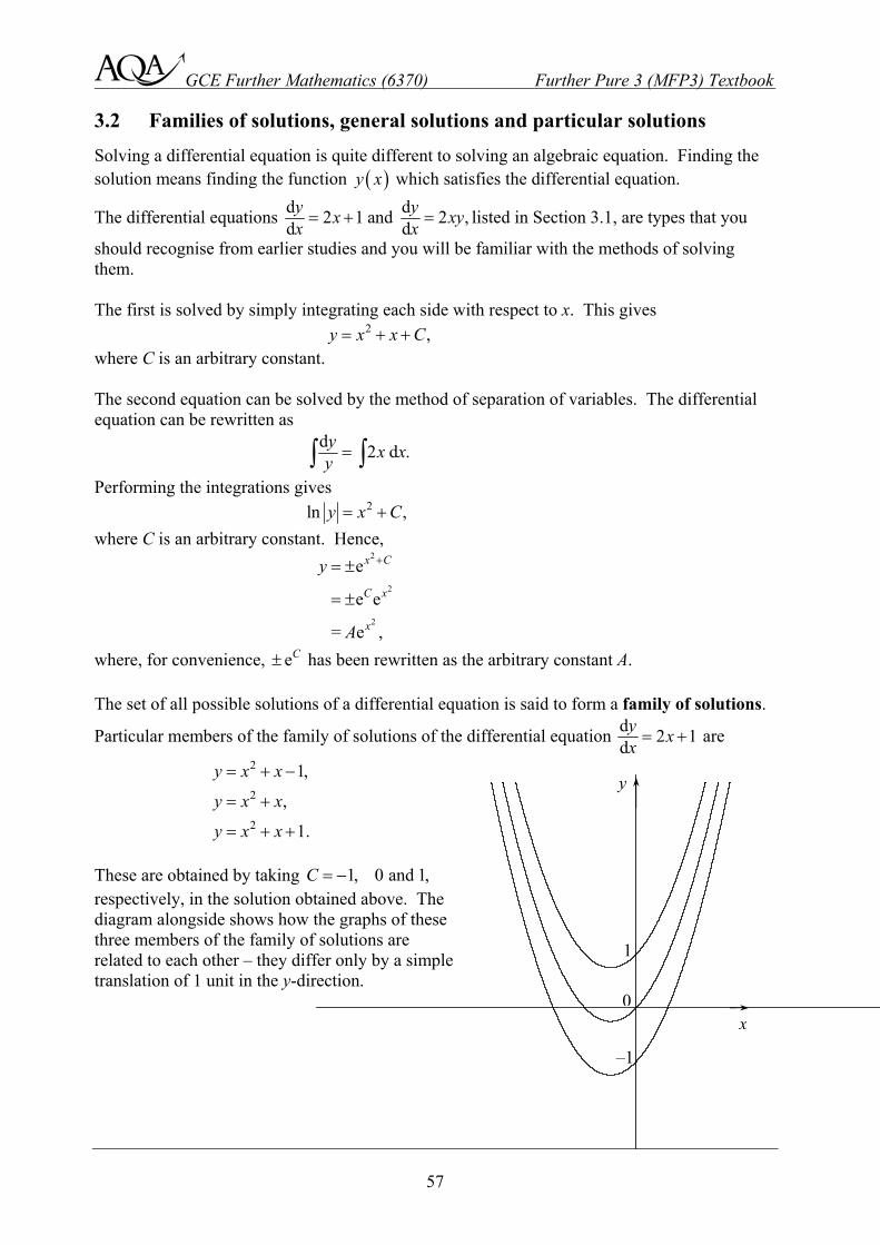
= + +
These are obtained by taking 1, 0 and 1,C = − respectively, in the solution obtained above. The diagram alongside shows how the graphs of these three members of the family of solutions are related to each other � they differ only by a simple translation of 1 unit in the y-direction.
x
y
1
0
�1

klmGCE Further Mathematics (6370) Further Pure 3 (MFP3) Textbook
58
Solutions that involve arbitrary constants are called general solutions because they represent the whole family of possible solutions. A solution which satisfies the differential equation but contains no arbitrary constants is called a particular solution. General solutions of first order differential equations always contain exactly one arbitrary constant, as will be seen in the cases dealt with in this chapter.
For the differential equation d 2 ,dy xyx = the general solution, as shown above, is
2e .xy A=
Examples of particular solutions are 2 2
e and 2e ,x xy y= = obtained by taking 1 and 2,A A= = respectively. In most of the applications of differential equations, a particular solution valid over some specified interval, such as 0 1 or 0,x x≤ ≤ ≥ is required. The required solution of a first order differential equation is often chosen in order to satisfy a given condition at an end point of an interval under consideration. For example, if the interval under consideration is 0,x ≥ the given condition might be ( )0 2.y = It will be shown later that general solutions of second order linear differential equations contain two arbitrary constants and therefore two conditions need to be specified to identify a particular solution. Such conditions are called boundary conditions or end conditions or initial conditions. The term �initial condition� is particularly appropriate in applications in which the independent variable is time t and a solution valid for 0t ≥ is required. Then 0t = marks the beginning of the period under consideration.

klmGCE Further Mathematics (6370) Further Pure 3 (MFP3) Textbook
59
Example 3.2.1
The function ( )y x satisfies the differential equation
2 2d 0, 1.dyx y xx − = ≥
(a) Find the general solution for ( ).y x
(b) Hence find the particular solution satisfying the boundary condition ( ) 11 .2y =
Solution
The differential equation can be written as
2
2d .dy yx x=
Separating the variables, this becomes
2 2d d ,y xy x
=∫ ∫
giving 1 1 ,Cy x− = − +
where C is an arbitrary constant.
Hence, 1 1 .Cxy x
−=
The general solution is therefore
.1xy Cx=−
Applying the boundary condition, ( ) 11 ,2y = gives
1 1 .2 1 C=−
Hence, 1.C = − The required particular solution is therefore
.1xy x=+
(a)
(b)

klmGCE Further Mathematics (6370) Further Pure 3 (MFP3) Textbook
60
Exercise 3B
1. The differential equation d ,dy kyx = where k is a constant, governs phenomena involving
growth ( )0k > or decay ( )0 .k <
Show that the general solution is e ,kxy C= where C is an arbitrary constant.
[You will find it useful to memorise this solution so that you can quote it when required.] 2. (a) Obtain the general solution of the differential equation
2d 0.dy xyx + =
(b) Find the particular solution which satisfies the condition ( )0 2.y = 3. (a) Obtain an equation representing the family of solutions of the differential equation
2d 1 , 0.d
y xx x= >
(b) Find the equation of the member of this family whose graph passes through the point (1, 0).
(c) Sketch this graph. 4. (a) Solve the differential equation
d 0, 0 2,dy y xx + = ≤ ≤
subject to the boundary condition ( )0 3.y =
(b) Verify that ( )2 0.406.y ≈ 5. A cyclist travelling on a level road stops pedalling and freewheels for 5 seconds. The
distance travelled by the cyclist in t seconds is x metres. The relationship between x and t while the cyclist is freewheeling can be modelled by the differential equation
( )2
d 250 .d 5xt t=
+
(a) Find the general solution of this differential equation.
(b) (i) State the appropriate initial condition to be satisfied by ( ).x t (ii) Find the particular solution satisfying this condition.
(c) Deduce that the cyclist travels 25 metres while freewheeling.

klmGCE Further Mathematics (6370) Further Pure 3 (MFP3) Textbook
61
3.3 Analytical solution of first order differential equations: integrating factors
The general first order linear differential equation may be expressed as d ,dy Py Qx + =
where P and Q are functions of x. A simple example is 2d ,dy y xx x− = which was included in the
list of differential equations in Section 3.1. Except in the special cases when both P and Q are constants or when one of these two functions is zero, differential equations of this type cannot be expressed in variables separated form; the method of separation of variables is therefore not available. However, there are two other analytical methods of solution which can be used, the first of which is as follows. If each side of the differential equation
ddy Py Qx + =
is multiplied by I, where I is a function of x, it becomes
d .dyI IPy IQx + =
The aim of this method is to choose I so that
( )d d .d dyI IPy Iyx x+ =
Since ( ) dd d ,d d dy IIy I yx x x= +
I must be chosen so that d .dI IPx = Hence
d d ,I P xI =∫ ∫
which gives ln dI P x= ∫ and therefore de .P xI ∫= ± It is usual to choose the positive sign (either will do) and hence The function I is obtainable provided that ( )P x can be integrated. Assuming that I has been found, the differential equation becomes
( )d .d
Iy IQx
=
Hence d ,Iy IQ x= ∫ giving the solution
( ) 1 d .y x IQ xI
= ∫
The function ( )I x is called an integrating factor because knowledge of this enables the equation to be solved.
de P xI ∫=

klmGCE Further Mathematics (6370) Further Pure 3 (MFP3) Textbook
62
Example 3.3.1
(a) Find the integrating factor of the differential equation 2d , where 0.dy y x xx x− = >
(b) Hence find
(i) the general solution, (ii) the particular solution satisfying the condition ( )1 0.y = Solution
In this case 1 .P x= − Hence, using the formula obtained above, the integrating factor is
1 d
ln
1ln
e
e
e
1
1 , since 0.
xx
x
x
I
x
xx
−
−
−
∫=
=
=
=
= >
Multiplying each side of the differential equation by the integrating factor gives
2d1 ,d
y y xx x x− =
which can be rewritten as
d .dy xx x
⎛ ⎞ =⎜ ⎟⎝ ⎠
Note that the left-hand side of this equation is ( )d ,d Iyx as it should be. The above
equation can be integrated at once giving
21 ,2y x Cx = +
where C is an arbitrary constant. The general solution of the differential equation is therefore
( )21 .2y x x C= +
Applying the condition ( )1 0y = gives
10 .2 C= +
Hence ( )21 1 and 1 .2 2C y x x= − = −
(a)
(b)(i)
(ii)

klmGCE Further Mathematics (6370) Further Pure 3 (MFP3) Textbook
63
There are some points to note about the application of this method.
• If the differential equation considered in Example 3.3.1 had been given in the form 3d ,d
yx y xx − = it would have been necessary, as a first step, to divide through by x to express
it in the standard form d .dy Py Qx + = It is essential to do this before attempting to find the
integrating factor.
• When the integrating factor I has been found, it is the standard form that is multiplied through by I, not the original form.
• When finding I, it will often be necessary to use the fact that ( ) ( )ln fe f ,x x= as in Example 3.3.1.
• When the differential equation (in standard form) is multiplied through by the integrating factor I, the left-hand side should then be expressible as ( )d .d Iyx
Example 3.3.2
Find the solution of the differential equation
( ) ( )d πcos sin 1, 0 ,d 2yx x y xx + = ≤ <
satisfying the boundary condition ( )0 1.y = Solution In standard form, the differential equation is
( )d tan sec .dy x y xx + =
The integrating factor is
tan d ln sece e sec .x x xI x∫= = =
Since sec 0x > when π0 , sec .2x I x≤ < =
Multiplying the differential equation (in standard form) throughout by sec x gives
( ) ( ) 2dsec sec tan sec ,dyx x x y xx + =
which can be written as ( ) 2d sec sec .d y x xx =
Hence, sec tan ,y x x C= +
where C is an arbitrary constant. In terms of sin x and cos ,x this can be expressed as
sin cos ,y x C x= +
and this is the general solution for y.
Applying the boundary condition, ( )0 1,y = gives 1 .C= Hence sin cos .y x x= +

klmGCE Further Mathematics (6370) Further Pure 3 (MFP3) Textbook
64
Exercise 3C
1. (a) Find the integrating factor of the differential equation d 2 4 , 0.dy y x xx x+ = >
(b) Hence find the general solution.
2. (a) Find the general solution of the differential equation 2d 2 e .dxy yx + =
(b) Hence find the particular solution satisfying the condition ( )0 0.y = 3. Solve the differential equation
2 d 1,dyx xyx + =
where 0,x > subject to the condition that ( )1 0.y = 4. Find the general solution of the differential equation
3d 2 ,dyx y xx − =
where 0.x > 5. (a) Show that sin x is an integrating factor of the differential equation
( )d cot , 0 π.dy x y x xx + = < <
(b) Hence find
(i) the general solution,
(ii) the particular solution satisfying the condition ( )π 0.2y =
6. Find the solution of the differential equation
( )d πtan 1, ,d 2y x y xx − = <
which is such that ( )0 1.y =
7. (a) Find the general solution of the differential equation 2d e , 0.dxy y x xx x
−− = >
(b) Hence find the particular solution which is such that y remains finite as .x →∞ 8. A curve is such that at any point ( ),x y on it, its gradient is .y x− The curve passes through
the point ( )0, 2 . Find the equation of the curve.

klmGCE Further Mathematics (6370) Further Pure 3 (MFP3) Textbook
65
3.4 Complementary functions and particular integrals
Linear differential equations in which the coefficients of y and its derivatives are constants occur frequently. The general first order differential equation of this type has the form
( )d f ,dya by xx + =
where a and b are constants. Such equations can be solved by finding an integrating factor but there is an alternative method which is sometimes easier to apply. The alternative method also has the advantage that it can be used to solve higher order linear differential equations with constant coefficients. These will be dealt with in Chapter 5. To understand the essentials of this alternative method, consider the particular case
d 2 e .dxy yx + =
The first step is to replace the right-hand side by zero giving
d 2 0.dy yx + =
This is called the reduced equation. Rewriting it as
d 2 ,dy yx = −
it can be seen that it is a standard decay equation for which the general solution is 2e ,xy C −= where C is an arbitrary constant. (See Exercise 3B, Question 1.) The next step is to try to find, by trial or inspection, a particular solution of the complete equation
d 2 e .dxy yx + =
Any function that satisfies this equation is sufficient. In this case, the form of the right-hand side suggests that exy A= is tried, where A is a constant to be found. Substituting this into the differential equation gives e 2 e e .x x xA A+ =
The terms in ex cancel giving 1 .3A = Hence 1 e3xy = is a particular solution.
The final step is to add the general solution of the reduced equation and the particular solution of the complete equation. This gives
2 1e e .3x xy C −= +
It is easy to verify that this function satisfies the complete equation (check this). As it also contains an arbitrary constant it is the required general solution. The general solution of the reduced equation is called the complementary function, and the particular solution of the complete equation is called a particular integral. The sum of the two gives the required general solution of the complete equation. These terms are often abbreviated to CF, PI and GS, respectively.

klmGCE Further Mathematics (6370) Further Pure 3 (MFP3) Textbook
66
In practice, finding a CF is straightforward, as it was in the example above. However, finding a PI is generally much more difficult and only when ( )f x takes certain simple forms is it likely
to be possible � this is the main drawback of this method. Fortunately, in applications ( )f x is often of a simple exponential, trigonometric or polynomial form and in these cases a PI can be found by using an appropriate trial function, as follows. Only the above cases and simple combinations of them need to be considered for the purposes of this course.
The steps in the procedure for solving differential equations of the form
( )d fdya by xx + =
can be summarised as follows.
• Find the GS of the reduced equation d 0.dya byx + = This solution is the CF, C.y
• Find a particular solution of the complete equation ( )d fdya by xx + = .
This function is a PI, P.y
• The GS of the complete equation is then C P.y y y= +
• If ( )f x is of the form e ,kxc where c and k are constants, try a PI of the form
e ,kxy a= where a is a constant to be found. The example used at the beginning of this section (to explain the method) illustrates this case. This fails when the CF has the same exponential form as the right-hand side of the differential equation. However, it will then be found that the trial function
ekxy ax= will provide a PI. Example 3.4.3 covers this more difficult case.
• If ( )f x is of the form cos or sin ,c kx c kx try a PI of the form cos sin ,y a kx b kx= +where a and b are constants to be found.
• If ( )f x is a polynomial of degree n, try a PI of the form 1 ,n ny ax bx −= + +" where a, b, � are constants to be found.

klmGCE Further Mathematics (6370) Further Pure 3 (MFP3) Textbook
67
Example 3.4.1
Find a PI of the differential equation d sin .dy y xx + =
Solution The appropriate trial function is cos sin .y a x b x= +
Substituting this into the differential equation gives
sin cos cos sin sin ,a x b x a x b x x− + + + =
i.e. ( ) ( )cos sin sin .b a x b a x x+ + − =
The constants a and b must be chosen so that 0 and 1.b a b a+ = − = This gives 1 1 and .2 2a b= − = Hence, the required PI is
1 1cos sin .2 2y x x= − +

klmGCE Further Mathematics (6370) Further Pure 3 (MFP3) Textbook
68
Example 3.4.2
Solve the differential equation 2d 2 2 3,dy y xx + = + given that ( )0 5.y =
Solution
The reduced equation is d 2 0dy yx + = for which the GS is 2e ,xy C −= where C is an arbitrary
constant. This is the CF.
The right-hand side of the complete equation is a polynomial of degree 2, so the appropriate trial function for a PI is 2 .y ax bx c= + + Differentiating this gives
d 2 .dy ax bx = +
Substituting these expressions for y and ddyx into the complete equation gives
2 22 2 2 2 2 3.ax b ax bx c x+ + + + = +
This may be expressed more conveniently as ( )2 22 2 2 2 3.ax a b x b c x+ + + + = +
Hence, comparing coefficients,
( )2 2,
2 0,2 3.
aa bb c
=
+ =
+ =
Thus 1, 1 and 2.a b c= = − = The PI is therefore 2 2.y x x= − +
Adding the CF and the PI, the GS of the complete equation is therefore
2 2e 2.xy C x x−= + − +
Applying the condition ( )0 5y = gives 5 2C= + and hence 3.C = The required solution is therefore 2 23e 2.xy x x−= + − + Note that a common mistake is to apply the end condition ( )0 5 in the example abovey⎡ ⎤=⎣ ⎦ to the CF (i.e. to the GS of the reduced equation). It is essential to apply the end condition to the GS of the complete equation.

klmGCE Further Mathematics (6370) Further Pure 3 (MFP3) Textbook
69
Example 3.4.3
Find the CF and a PI of the differential equation 12d2 3e .d
xy yx − = Hence write down the GS.
Solution
The reduced equation is d2 0,dy yx − =
i.e. d 1 .d 2y yx =
The GS of this is 12e xy C= and this is the required CF of the complete equation.
To find a PI, note first that the CF has the same exponential form as the right-hand side of the
given differential equation. The appropriate trial function for the PI is therefore not 12e xa but
12e .xy ax=
Differentiating this using the product rule gives
1 12 2d 1 e e .d 2
x xy ax ax = +
Substituting y and ddyx into the complete differential equation,
1 1 1 12 2 2 2e 2 e e 3e .x x x xax a ax+ − =
The terms in 12e xax cancel and it can be seen that 3 .2a = Hence the PI is
123 e .2
xy x=
The GS of the complete equation is therefore
1122 3e e .2
xxy C x= +

klmGCE Further Mathematics (6370) Further Pure 3 (MFP3) Textbook
70
Note: It is interesting to see why the trial function 12e xy a= will not provide a PI in this case.
Substituting this into the differential equation gives
( )1 1 12 2 212 e e 3e .2
x x xa a− =
However, the left-hand side is zero so there is no value of a for which the differential equation
can be satisfied. Of course, the left-hand side must be zero because 12e xa is a solution of the
reduced equation! Exercise 3D
1. Find a particular integral of each of these differential equations.
(a) 2d 3 9 1dy y xx + = + (b) d2 3d
y y xx − = −
(c) d 3 sin 2cosdy y x xx + = + (d) d2 2cosd
y y xx − =
(e) 3d 3 3edxy yx + = (f) 3d 3 3ed
xy yx − =
(g) d2 4 8 edxy y xx
−+ = +
2. (a) Find the complementary function and a particular integral of the differential equation
d 3 6.dy yx − =
(b) Hence obtain the solution satisfying the condition ( )1 0.y = 3. (a) Find the complementary function and a particular integral of the differential equation
2d 2 e .dxy yx − =
(b) Hence obtain the solution satisfying the condition ( )0 2.y = 4. Solve the differential equation
d sin 2 ,dy y xx + =
subject to the condition ( )0 1.y =

klmGCE Further Mathematics (6370) Further Pure 3 (MFP3) Textbook
71
3.5 Transformations of non-linear differential equations to linear form
It is sometimes possible to transform a first order non-linear differential equation into one of first order linear form by means of a suitable substitution. If the solution of the transformed equation can be found, the solution of the non-linear equation can be deduced from it. The example which follows shows how this technique may be used. Example 3.5.1
The function ( )y x satisfies the differential equation d 2 2 , 1.dy y x y xx x= + ≥
(a) Show that the substitution 2y u= transforms the differential equation into d .du u xx x− =
(b) Find the general solution for u.
(c) Hence obtain the solution for y satisfying the boundary condition ( )1 0.y = Solution
Differentiating each side of 2y u= with respect to x gives d d2 .d dy uux x=
Hence the differential equation transforms to
2d 22 2 ,d
u uu xux x= +
which can be written as d .du u xx x− =
The integrating factor for the differential equation above is
( )1 d ln 1 1e e 1 .
x xx x x xxx− −∫ = = = ≥ ⇒ =
Multiplying the differential equation throughout by this factor gives
21 d 1.d
u ux x x
− =
Hence, ( )d 1,du
x x =
which gives ,u x Cx = +
where C is an arbitrary constant. The general solution for u is therefore ( ).u x x C= + Since 2 ,y u= the general solution for y is
( )22 .y x x C= +
Applying the boundary condition, ( )1 0,y = gives ( )20 1 .C= + Hence 1C = − and
therefore ( )22 1 .y x x= −
(a)
(b)
(c)

klmGCE Further Mathematics (6370) Further Pure 3 (MFP3) Textbook
72
Exercise 3E
1. (a) Show that the substitution 1y u= transforms the differential equation
2d 2 ,dy y yx x− = −
where 0, intox >
d 2.du ux x+ =
(b) Obtain the general solution for u and hence the general solution for y. 2. (a) Show that the substitution y x u− = transforms the differential equation
d e 1dy xy
x−+ =
into d e 0.duu
x + =
(b) Find the general solution for u. (c) Hence obtain the solution for y satisfying the condition ( )0 0.y = (d) State the range of values of x for which the solution in part (c) is valid. 3. The function ( )y x satisfies the differential equation
2d e 2 , 1.d
yy xx xx+ = ≥
(a) Show that the substitution lny u= − transforms the differential equation into
2d 2 1 .du ux x x+ =
(b) Obtain the general solution for u. (c) Hence obtain the solution for y satisfying the boundary condition ( )1 0.y =

klmGCE Further Mathematics (6370) Further Pure 3 (MFP3) Textbook
73
Miscellaneous exercises 3
1. (a) Show that the integrating factor of the differential equation
( )d πtan 2 cos , 0 ,d 2y x y x x xx + = ≤ <
is 1 .cos x
(b) Hence obtain the solution for y satisfying the boundary condition that ( )0 3.y =
[AQA 1999]
2. (a) For the differential equation d sin ,dy y xx + = find
(i) the complementary function,
(ii) a particular integral. (b) Hence, or otherwise, solve the equation given that 1 when 0.y x= =
[JMB 1991] 3. A curve C in the x�y plane passes through the point ( )1,0 . At any point ( ),x y on C,
d e .dxy yx
−+ =
(a) Find the general solution of this differential equation. (b) (i) Hence find the equation of C, giving your answer in the form ( )f .y x=
(ii) Write down the equation of the asymptote of C. [NEAB 1998]
4. (a) Show that the integrating factor of the differential equation
d 1 , 1,d 1y y x xx x− = >
−
is 1 .1x −
(b) Find the solution of this differential equation, given that ( )2 1.y = Express your answer
in the form ( )f .y x= [AQA 2001]

klmGCE Further Mathematics (6370) Further Pure 3 (MFP3) Textbook
74
5. The differential equation 3d 2 8dy y xx + = has a particular integral of the form
3 2 ,ax bx cx d+ + +
where a, b, c and d are constants. (a) Find the values of a, b, c and d.
(b) Find the complementary function.
(c) Obtain the solution of the differential equation which satisfies the condition ( )0 0.y = 6. A curve in the region 0x > of the x�y plane is such that the tangent at every point ( ),x y on
it intersects the y-axis at ( )0, .x
(a) Show that d .dyx y xx = −
(b) Hence find the equation of the curve which possesses this property and which passes
through the point ( )1, 2 .− (c) Show that this curve approaches the origin as 0.x →
[NEAB 1994]
7. (a) Show that the substitution 1y u= transforms the differential equation
2d ln , 0,dyx y y x xx + = >
into the differential equation
d ln .du u xx x x− = −
(b) Find the general solution of the equation for u.
(c) Hence find y in terms of x, given that 1 when 1.2y x= =
[JMB 1988]
8. (a) Show that the substitution 13y u
−= transforms the differential equation
3 4d 2 ,dyy x x yx− =
where 0,x > into
2d 3 6 .du u xx x+ =
(b) Use the above result to find the general solution of the differential equation for y.
[JMB 1990]

klmGCE Further Mathematics (6370) Further Pure 3 (MFP3) Textbook
75
Chapter 4: Numerical Methods for the Solution of First Order Differential Equations 4.1 Introduction
4.2 Euler�s formula
4.3 The mid-point formula
4.4 The improved Euler formula
4.5 Error analysis: some practical considerations
This chapter gives an introduction to numerical methods for solving first order differential equations. When you have completed it, you will: • be familiar with the standard notation used; • be familiar with the methods which use Euler�s formula, the mid-point formula and Euler�s
improved formula; • know how the above formulae can be derived both geometrically and analytically; • be aware of the principal sources of error in the methods described; • know how the accuracy of a numerical solution can be estimated.
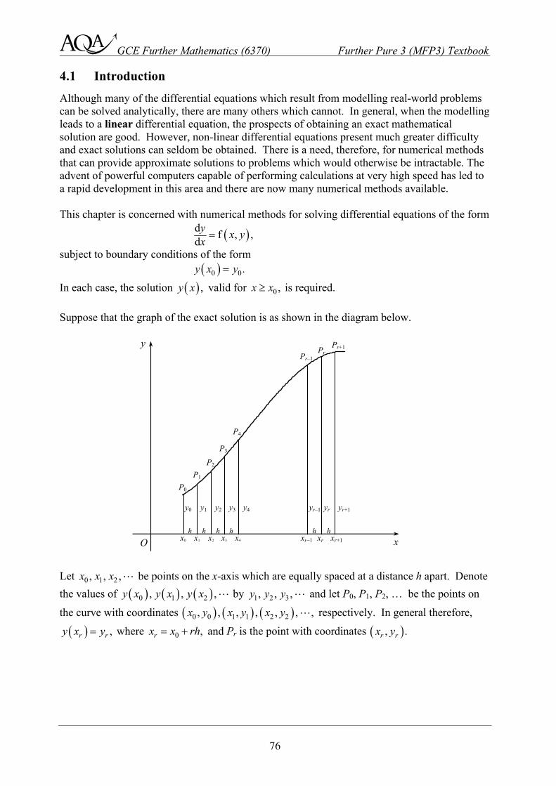
klmGCE Further Mathematics (6370) Further Pure 3 (MFP3) Textbook
76
4.1 Introduction
Although many of the differential equations which result from modelling real-world problems can be solved analytically, there are many others which cannot. In general, when the modelling leads to a linear differential equation, the prospects of obtaining an exact mathematical solution are good. However, non-linear differential equations present much greater difficulty and exact solutions can seldom be obtained. There is a need, therefore, for numerical methods that can provide approximate solutions to problems which would otherwise be intractable. The advent of powerful computers capable of performing calculations at very high speed has led to a rapid development in this area and there are now many numerical methods available. This chapter is concerned with numerical methods for solving differential equations of the form
( )d f , ,dy x yx =
subject to boundary conditions of the form ( )0 0.y x y=
In each case, the solution ( ) ,y x valid for 0 ,x x≥ is required. Suppose that the graph of the exact solution is as shown in the diagram below. Let 0 1 2, , ,x x x " be points on the x-axis which are equally spaced at a distance h apart. Denote the values of ( ) ( ) ( )0 1 2, , ,y x y x y x " by 1 2 3, , ,y y y " and let P0, P1, P2, � be the points on
the curve with coordinates ( ) ( ) ( )0 0 1 1 2 2, , , , , , ,x y x y x y " respectively. In general therefore,
( ) ,r ry x y= where 0 ,rx x rh= + and Pr is the point with coordinates ( ), .r rx y
O
y
x x0 x1 x2 x3 x4 xr�1 xr xr+1
Pr�1
Pr+1Pr
P4
P3 P2
P1 P0
y0 y1 yr�1 y2 y3 y4 yr yr+1
h h h h h h

klmGCE Further Mathematics (6370) Further Pure 3 (MFP3) Textbook
77
The basic idea of all the numerical methods is to use a step-by-step procedure to obtain approximations to the values of 1 2 3, , ,y y y " successively. The interval, h, between successive x-values is called the step length. Some of the methods of obtaining these approximations are suggested by geometrical considerations of the graph. Three such methods will be described in the sections that follow. Later in the chapter, consideration will be given to the accuracy of the values obtained. It is important to become thoroughly familiar with the standard notation introduced above. Exercise 4A will help with this. Exercise 4A
Suppose that the differential equation to be solved is
3 3d , 1,dy x y xx = + ≥
and that the boundary condition is ( )1 2.y =
Suppose also that the values of ( ) ( )1.1 , 1.2 ,y y ( ), 2.0y" are required. In this case:
(a) state the values of 0 0 1 2, , , and ;x y h x x
(b) state which of the values of y that are required correspond to 1 10and ;y y
(c) evaluate ( )0 0f , .x y

klmGCE Further Mathematics (6370) Further Pure 3 (MFP3) Textbook
78
4.2 Euler�s formula
Consider again the diagram in Section 4.1. One simple way of obtaining an approximation to the value of 1y is to assume that the part of the curve between P0 and P1 is a straight line
segment with gradient equal to the gradient of the curve at P0. Since ( )d f , ,dy x yx = the gradient
of the curve at P0 is ( )0 0f , .x y Hence, with this approximation,
( )1 00 0f , ,y y x yh
−=
giving ( )1 0 0 0f , .y y h x y= + Using this approximation to obtain the value of y at P1, the process can be repeated, assuming that the part of the curve between P1 and P2 is a straight line segment with gradient equal to the
value of ddyx at P1. This gives
( )2 1 1 1f , .y y h x y= +
Continuing in this way gives, in general,
( )1 f , , 0,1, 2, .r r r ry y h x y r+ = + = " This is Euler�s formula. Successive calculation of values of y using this formula is known as Euler�s method. It is clear from the nature of the linear approximation on which this method is based that the step length h needs to be fairly small to achieve reasonable accuracy.

klmGCE Further Mathematics (6370) Further Pure 3 (MFP3) Textbook
79
Example 4.2.1
The function ( )y x satisfies the differential equation
( )d sindy x yx = +
and the condition ( )1 0.y =
Use Euler�s formula to estimate the values of ( ) ( ) ( )1.1 , 1.2 and 1.3 ,y y y giving the answers to four decimal places. Solution In this case, ( ) ( )0 01, 0, 0.1 and f , sin .x y h x y x y= = = = +
Also ( ) 11.1 ,y y= ( ) 21.2y y= and ( ) 31.3 .y y= Using Euler�s formula:
( )1 0 0 0sin0.1sin10.0841470.0841 to four d.p.
y y h x y= + +
=≈=
( )( )
2 1 1 1sin
0.084147 0.1sin 1.1 0.0841470.1767650.1768 to four d.p.
y y h x y= + +
= + +
≈=
( )( )
3 2 2 2sin
0.176765 0.1sin 1.2 0.1767650.2748890.2749 to four d.p.
y y h x y= + +
= + +
≈=
Note that at each stage after the first in the above calculations, the previous value of y to six decimal places is used instead of the four-decimal place rounded answer. If this is not done, accuracy to four decimal places is not guaranteed. For example, the use of 1 0.0841y = would have given 2 0.1767.y = It is recommended that working is always carried out to two decimal places more than the number of decimal places required in the final answer.

klmGCE Further Mathematics (6370) Further Pure 3 (MFP3) Textbook
80
Exercise 4B
1. The function ( )y x satisfies the differential equation
( )d lndy x yx = +
and the condition ( )1 1.y = Use Euler�s formula with a step length of 0.1 to obtain approximations to the values of
( ) ( ) ( ) ( ) ( )1.1 , 1.2 , 1.3 , 1.4 and 1.5 .y y y y y Give your answers to three decimal places. 2. The function ( )y x satisfies the differential equation
ddyy x yx = +
and the condition ( )0 1.y =
Use Euler�s method with a step length of 0.25 to obtain an estimate of the value of ( )1 .y Give your answer to three decimal places.
3. The function ( )y x satisfies the differential equation
( )d f ,dy x yx =
where ( ) ( )2f , e e .x yx y = +
The value of ( )0y is zero.
(a) Use of the Euler formula gave 1 0.05.y = Determine the value that was used for the step length h .
(b) Show that, with this value for h, the Euler formula gives 2 0.103y = to three decimal places.
(c) Calculate the value of 3y to three decimal places.

klmGCE Further Mathematics (6370) Further Pure 3 (MFP3) Textbook
81
4.3 The mid-point formula
The diagram below shows three points, Pr�1, Pr and Pr+1, on part of the curve representing the
solution of the differential equation ( )d f , .dy x yx =
Provided that the three points are reasonably close together, the gradient of the line segment joining Pr�1 and Pr+1 will be approximately the same as the gradient of the tangent to the curve
at Pr . Since ( )d f ,d r ry x yx = at Pr , this approximation gives
( )1 1 f , .2r r
r ry y x yh+ −−
=
Hence, ( )1 1 2 f , .r r r ry y h x y+ −= +
This is the mid-point formula. As with Euler�s formula, the mid-point formula can be used to calculate values of y successively, but at each stage the previous two values of y are required. In particular, putting
1r = gives ( )2 0 1 12 f , .y y h x y= +
Since only the value of 0y is known initially, it is necessary to calculate 1y by some other method before the application of the mid-point formula can begin. Euler�s formula may be used for this purpose. It will be shown later that, for a given step length h, the mid-point formula is more accurate than Euler�s formula.
O
y
x xr�1 xr+1xr
yr�1 yr+1yr
h h
Pr�1
Pr+1 Pr

klmGCE Further Mathematics (6370) Further Pure 3 (MFP3) Textbook
82
Example 4.3.1
The function ( )y x satisfies the differential equation
d 1dy xyx = +
and the condition ( )0 1.y =
Use the mid-point formula with a step length of 0.25 to obtain an approximate value for ( )1y
to three decimal places. Take ( )0.25y to be the value given by Euler�s formula. Solution In this case, ( )0 00, 1, 0.25 and f , 1 .x y h x y xy= = = = + Using Euler�s formula,
( ) ( )( )
1 0 0 00.25 1
1 0.25 11.25.
y y y h x y= = + +
= + ×
=
The mid-point formula gives:
( ) ( )( )
2 0 1 10.5 2 1
1 0.5 1 0.25 1.25
1.77951
y y y h x y= = + +
= + + ×
≈
( ) ( )( )
3 1 2 20.75 2 1
1.25 0.5 1 0.5 1.77951
2.22163
y y y h x y= = + +
= + + ×
≈
( ) ( )( )
4 2 3 31 2 1
1.77951 0.5 1 0.75 2.22163
2.924922.925 to three decimal places.
y y y h x y= = + +
= + + ×
≈=

klmGCE Further Mathematics (6370) Further Pure 3 (MFP3) Textbook
83
Exercise 4C
1. The function ( )y x satisfies the differential equation
3 3ddy x yx = +
and the condition ( )1 1.y = (a) Using a step length of 0.1 in the Euler formula ( )1 f , ,r r r ry y h x y+ = + obtain estimates of the values of y when 1.1x = and 1.2.x = (b) Use the mid-point formula, ( )1 1 2 f , ,r r r ry y h x y+ −= + with 0.1h = and your value of 1y obtained in part (a), to calculate an improved estimate
of the value of y when 1.2.x = 2. The function ( )y x satisfies the differential equation
d cosdy xyx =
and the condition ( )1 2.y = (a) Verify that the Euler formula with a step length of 0.25 gives ( )1.25 1.89596y = to five
decimal places. (b) Use the mid-point formula with a step length of 0.25 to obtain an estimate of the value
of ( )2 .y Give your answer to three decimal places. 3. The function ( )y x satisfies the differential equation
( )1
2 2 2d 1dy x yx = + +
and the condition ( )0 0.y = (a) Given that in this case 1 1,y y− = − show that the mid-point formula gives 1 ,y h= where h
is the step length. (b) Use the mid-point formula with 0.1h = to obtain an approximation to the value of
( )0.5 .y Give your answer to three decimal places.

klmGCE Further Mathematics (6370) Further Pure 3 (MFP3) Textbook
84
4.4 The improved Euler formula
The Euler formula derived in Section 4.2 is based on the assumption that the gradient of the line segment joining any two successive points, rP and 1,rP + on the graph of ( )y x is equal to
the value of ddyx at .rP Another formula, which is considerably more accurate than Euler�s, can
be obtained by assuming that the gradient of 1r rP P + is equal to the average of the values of ddyx
at rP and 1.rP + With this assumption,
( ) ( )11 1
1 f , f , .2r r
r r r ry y x y x yh+
+ +−
⎡ ⎤= +⎣ ⎦
Hence, ( ) ( )1 1 1f , f , .2r r r r r rhy y x y x y+ + +⎡ ⎤= + +⎣ ⎦
This formula cannot be used directly to calculate 1ry + because 1ry + is needed in order to evaluate ( )1 1f ,r rx y+ + on the right-hand side. To overcome this problem, 1ry + on the right-hand
side is replaced by a first estimate, denoted by *1 ,ry + giving
( ) ( )*1 1 1f , f , .2r r r r r rhy y x y x y+ + +⎡ ⎤= + +⎣ ⎦
There are a number of ways of obtaining a value for *1 .ry + The simplest is to use Euler�s
formula, giving ( )*
1 f , .r r r ry y h x y+ = + Using this expression together with the previous one for 1ry + constitutes the improved Euler method. It is sometimes called a predictor�corrector method because Euler�s formula gives an initial prediction of 1ry + and this is followed by the calculation of a corrected value. Note, however, that �corrected� here should not be interpreted literally � the new value of 1ry + will almost invariably be more accurate than the first estimate, but as the method is based on approximations there will still be some error involved.

klmGCE Further Mathematics (6370) Further Pure 3 (MFP3) Textbook
85
Example 4.4.1
The function ( )y x satisfies the differential equation
( )d ln , 1.dy x y xx = + ≥
The boundary condition is ( )1 1.y = Use the improved Euler method with a step length of 0.25
to estimate the value of ( )1.5y to three decimal places. Solution In this case, ( ) ( )0 01, 1, 0.25 and f , ln .x y h x y x y= = = = + Using Euler�s formula, the first estimate of 1y is
( )*
1 0 0 0ln1 0.25ln 21.17329.
y y h x y= + +
= +≈
Hence, using the expression derived above for 1,ry + with 0,r =
( ) ( )( )
*1 0 0 0 1 1ln ln21 0.125 ln 2 ln 1.25 1.17329
1.19728.
hy y x y x y⎡ ⎤= + + + +⎣ ⎦⎡ ⎤= + + +⎣ ⎦
≈
Observe that the �corrected� value, 1,y differs from the first estimate, *
1,y as is to be expected. The procedure can now be repeated to obtain 2y (i.e. the value of ( )1.5y ). Using Euler�s formula, the initial estimate is
( )
( )*2 1 1 1ln
1.19728 0.25ln 1.25 1.197281.42102.
y y h x y= + +
= + +
≈
Hence, ( ) ( )( ) ( )
*2 1 1 1 2 2ln ln2
1.19728 0.125 ln 1.25 1.19728 ln 1.5 1.42102
1.443.
hy y x y x y⎡ ⎤= + + + +⎣ ⎦⎡ ⎤= + + + +⎣ ⎦
≈
Again, note that 2y differs slightly from *2.y

klmGCE Further Mathematics (6370) Further Pure 3 (MFP3) Textbook
86
Alternative way of applying Euler�s improved method The formulae comprising the improved Euler method can be expressed in a different way. Substituting the expression obtained for *
1ry + into the expression for 1ry + gives
( ) ( )( )1 1f , f , f , .2r r r r r r r rhy y x y x y h x y+ +⎡ ⎤= + + +⎣ ⎦
Noting that 1 ,r rx x h+ = + this can be expressed as
( )1 1 21 ,2r ry y k k+ = + +
where ( )1 f ,r rk h x y=
and ( )2 1f , .r rk h x h y k= + + These expressions are quoted in the AQA Formulae Booklet, together with Euler�s formula. The example which follows shows how these expressions can be used as an alternative to the procedure used in Example 4.4.1 . Example 4.4.2
The function ( )y x satisfies the differential equation
( )d f , ,dy x yx =
where ( ) 2f , 2 3 2 , 0.x y x y x= + − ≥
The boundary condition is ( )0 5.y =
(a) Use the improved Euler method, with 0.25,h = to calculate approximations to the values of ( )0.25y and ( )0.5 .y
(b) The exact solution of the differential equation (obtained in Chapter 3, example 3.4.2) is
( ) 2 23e 2.xy x x x−= + − +
Calculate, to two significant figures, the percentage error in the value of ( )0.5y obtained in part (a).
Solution
The solution can be conveniently set out in tabular form.
r xr yr k1 rx h+ 1ry k+ k2 1ry +
0 0 5 �1.75 0.25 3.25 �0.84375 3.703125
1 0.25 3.703125 �1.0703125 0.5 2.6328125 �0.44140625 2.947266
(a)

klmGCE Further Mathematics (6370) Further Pure 3 (MFP3) Textbook
87
The entries on the first row are obtained as follows. It is given that ( )0 5,y = which implies that 0 0x = and 0 5.y = The formula for 1,k with 0,r = gives ( )
( )1 0 0
20 0
f ,
0.25 2 3 2
1.75.
k h x y
x y
=
= + −
= −
The next two entries in the table are 0 0.25x h+ = and 0 1 3.25.y k+ = The formula for 2 ,k with 0,r = gives ( )
( ) ( ){ }2
2
0.25f 0.25, 3.25
0.25 2 0.25 3 2 3.25
0.84375.
k =
= + − ×
= −
The formula for 1,ry + with 0,r = gives
( )
( )
1 0 1 212
15 1.75 0.8437523.703125.
y y k k= + +
= + − −
=
On the second row, the first two entries are 1 0 0.25x x h= + = and 1 3.703125y = (transferred from row 1). Then ( )
( ) ( ){ }1 1 1
2
f ,
0.25 2 0.25 3 2 3.703125
1.0703125.
k h x y=
= × + − ×
= −
The entries for 1x h+ and 1 1y k+ are straightforward with the values as shown. These give ( )
( ) ( )2
2
0.25f 0.5, 2.6328125
0.25 2 0.5 3 2 2.6328125
0.44140625.
k =
⎡ ⎤= × + − ×⎣ ⎦= −
Finally, ( )
( )
2 1 1 212
13.703125 1.5117187522.947266 to six d.p.
y y k k= + +
= + −
=
The exact solution quoted gives
( ) 1 22 0.5 3e 0.5 0.5 2
2.853638 to six d.p.y y −= = + − +
=
Hence the error in the value obtained in part (a) is
2.947266 2.853638 100% 3.3%.2.853638− × ≈
(b)

klmGCE Further Mathematics (6370) Further Pure 3 (MFP3) Textbook
88
Exercise 4D
1. The function ( )y x satisfies the differential equation
( )d lndy xyx =
and the condition (2) 1.y = An estimate of the value of ( )3y to three decimal places is required.
(a) Use the improved Euler method with a step length of 0.25 to obtain this estimate, setting out your working in a similar way to that of Example 4.4.1.
(b) Repeat the calculations using the alternative method of working as shown in
Example 4.4.2. 2. The function ( )y x satisfies the differential equation
2 2d ed
x yyx
+=
and the condition (0) 0.y =
Use the improved Euler method with a step length of 0.2 to obtain an approximate value of ( )0.4 .y Give your answer to three decimal places.
3. The function ( )y x satisfies the differential equation
( )d f , ,dy x yx =
where ( ) ( )2f , cos .x y x y= + When 1, 1.x y= = (a) Use the Euler formula with a step length of 0.1 to obtain an estimate of the value of
( )1.1 .y (b) Obtain a second estimate of the value of ( )1.1y by using the improved Euler formula
( ) ( )*1 1 1f , f ,2r r r r r rhy y x y x y+ + +⎡ ⎤= + +⎣ ⎦
taking *1y to be the value obtained for the first estimate of ( )1.1y in part (a).
(c) Repeat the calculation in part (b) to obtain a third estimate of the value of ( )1.1 ,y taking
*1y to be the value obtained for the second estimate.
(d) Verify that the second and third estimates of ( )1.1y are in agreement to three decimal
places.

klmGCE Further Mathematics (6370) Further Pure 3 (MFP3) Textbook
89
4.5 Error analysis: some practical considerations
The three numerical formulae that were used for solving the differential equation ( )d f ,dy x yx =
were derived by geometrical considerations. They can also be derived analytically. There is some advantage in this alternative method because it enables some insight to be gained into the errors involved in the approximations. The Maclaurin series for ( )y h is
( ) ( ) ( ) ( ) ( )2 3
0 0 0 0 ,2! 3!h hy h y h y y y′ ′′ ′′′= + + + +…
where, as usual, , , ,y y y′ ′′ ′′′… denote derivatives of first order, second order, third order, � . If the origin is transferred to the point ,rx this becomes
( ) ( ) ( ) ( ) ( )2 3
,2! 3!r r r r rh hy x h y x h y x y x y x′ ′′ ′′′+ = + + + +…
which is Taylor�s series. (See also exercise 1B, question 6). Using the notation introduced in Section 4.1, and noting that ( ) ( )f , ,r r ry x x y′ = the Taylor series may be expressed as
( ) ( ) ( )2 3
1 f , .2! 3!r r r r r rh hy y h x y y x y x+ ′′ ′′′= + + + +…
If h is assumed to be sufficiently small for terms in 2 3, ,h h " to be negligible, then the series reduces to ( )1 f , ,r r r ry y h x y+ = + which is Euler�s formula. Taylor�s series can also be used to step backwards from ( )1to 1r rx x r− ≥ by replacing h by
.h− This gives
( ) ( ) ( )2 3
1 f , .2! 3!r r r r r rh hy y h x y y x y x− ′′ ′′′= − + − +…
Subtracting this from the series for 1ry + and neglecting all terms in 3h and higher powers, gives ( ) ( )1 1 2 f , , 1 .r r r ry y h x y r+ −= + ≥ This is the mid-point formula derived in Section 4.3. To obtain the improved Euler formula, first replace y by y′ in the Taylor series. This gives
( ) ( ) ( ) ( )2
,2!r r r rhy x h y x h y x y x′ ′ ′′ ′′′+ = + + +…
which may be expressed as
( ) ( ) ( ) ( )2
1 1f , f , .2!r r r r r rhx y x y h y x y x+ + ′′ ′′′= + + +…
klmGCE Further Mathematics (6370) Further Pure 3 (MFP3) Textbook
90
Multiplying each side of this equation by 12 h and subtracting the result from the above Taylor
series for 1ry + gives
( ) ( )1 1 1f , f ,2 2r r r r r rh hy x y y x y+ + +− = + + terms in 3h and higher powers.
If the terms in 3h and higher powers are neglected, this becomes, after rearrangement,
( ) ( )1 1 1f , f , .2r r r r r rhy y x y x y+ + +⎡ ⎤= + +⎣ ⎦
This is the improved Euler formula. The error incurred by neglecting terms in an expansion is called the truncation error. The derivations above show that the truncation error in Euler�s formula is greater than that in the mid-point formula and the improved Euler formula because an extra term (that in 2h ) is neglected. Hence, for a given step length h, Euler�s method cannot be expected to achieve the same accuracy as the other two methods. In addition to the truncation error, for all values of 1,r ≥ another error will be incurred in the calculation of 1ry + because an approximate value of ry has to be used in the evaluation of
( )f , .r rx y For example, whichever method is used, in order to calculate 2y , the value of
( )1 1f ,x y is required and only an approximate value of 1y is available. As the calculation of y-values progresses, errors of this type sometimes decay but they can also sometimes become increasingly large. In the latter case, it will usually become apparent by wildly erratic behaviour of the solution being generated � the method is then said to be unstable. It is often difficult to determine with complete certainty the accuracy of y-values that have been calculated by a numerical method. However, improved accuracy is almost invariably achieved by using a smaller step length, though this is at the expense of having to take more steps to reach a given end point. To estimate the order of accuracy of a solution, the usual procedure is to reduce the step length to half its previous value and repeat the calculations. If the results obtained are the same to, say, three decimal places, then it is usually safe to assume that they are correct to this order of accuracy. Of the three methods discussed, Euler�s improved method is best as it achieves reasonable accuracy and has a good record for stability. It is, in fact, the simplest of a class of methods � called Runge-Kutta methods � which are amongst the most reliable. In practice, nowadays all numerical methods for solving differential equations are programmed to be carried out on a computer. It is therefore relatively easy to experiment with different formulae and to see how changing the step length affects the solution generated.

klmGCE Further Mathematics (6370) Further Pure 3 (MFP3) Textbook
91
Exercise 4E
1. The function ( )y x satisfies the differential equation
d 2dy yx x= +
and the condition ( )1 0.y =
(a) Apply Euler�s formula twice with a step length of 0.2 to calculate the value of ( )1.4y to three decimal places.
(b) Repeat the calculations using four steps with a step length of 0.1.
(c) Use the mid-point formula with a step length of 0.2 to obtain the value of ( )1.4y to
three decimal places. Take the value of ( )1.2y to be that obtained in part (a).
(d) Use the improved Euler method with a step length of 0.2 to obtain the value of ( )1.4y to three decimal places.
(e) Verify that the exact solution of this problem is 2 ln .y x x=
(f) Hence calculate, to one decimal place, the percentage errors in the values of ( )1.4y obtained in parts (a) � (d).
(g) Comment on the results of the error calculations in part (f). 2 Use Taylor�s series to show that
( ) ( ) ( ) ( )2
.2!r r r rhy x h y x h y x y x′ ′ ′′ ′′′− = − + +"
Deduce that, when ( ) ( )f , ,y x x y′ =
( ) ( ) ( ) 21 1f , f , terms in and higher powers.r r r r rh y x x y x y h− −′′ = − +
Hence show that when terms in 3h and higher powers are neglected,
( ) ( )1 1 1+ 3f , f , .2r r r r r rhy y x y x y+ − −⎡ ⎤= −⎣ ⎦
3. The expression for 1ry + obtained in Question 2 is just one of several other formulae that
may be used to obtain numerical solutions of differential equations of the form
( )d f , .dy x yx =
(a) Apply this formula to the problem in Question 1 above, using a step length of 0.2, to
calculate the value of ( )1.4 .y Take the value of ( )1.2y to be that obtained using Euler�s formula with a step length of 0.2.
(b) By continuing the calculation with a step length of 0.2, show that the formula gives
( )2.0 2.722.y ≈
klmGCE Further Mathematics (6370) Further Pure 3 (MFP3) Textbook
92
Miscellaneous exercises 4
1. The function ( )y x satisfies the differential equation
( )1
3 3 2ddy x yx = +
and the condition ( )1 0.5.y = (a) Use the Euler formula, ( )1 f , ,r r r ry y h x y+ = +
with 0.1,h = to show that ( )1.1 0.606y = to three decimal places. (b) Use the mid-point formula, ( )1 1 2 f , ,r r r ry y h x y+ −= +
with 0.1,h = to find an approximate value for ( )1.3y giving your answer to three decimal places.
[AQA, 2001] 2. The function ( )y x satisfies the differential equation
( )d 4dy x y yx = + −
and the condition ( )1 2.y = (a) Use the Euler formula, ( )1 f , ,r r r ry y h x y+ = + to show that ( ) ( )1 2 1 .y h h+ ≈ − (b) (i) Denoting the value for ( )1y h+ obtained in part (a) by *
1 ,y show that
( ) ( )* 21 1f , 2 1 .x y h= − −
(ii) Hence obtain an improved estimate for the value of ( )1y h+ using the formula
( ) ( )*11 1 12 f , f ,r r r r r ry y h x y x y+ + +
⎡ ⎤= + +⎣ ⎦
giving your answer in the form
( ) 31 ,a h bh− +
where a and b are numbers to be found. [AQA, 2000]

klmGCE Further Mathematics (6370) Further Pure 3 (MFP3) Textbook
93
3. (a) (i) Show that the integrating factor of the differential equation
2 2d 1 , 1,d 1 1
y x y xx x x− = <
− −
is 21 .x− (ii) Hence, or otherwise, solve the differential equation given that 0x = when 0.y =
(iii) Show that when 0.5,x = π .3 3
y =
(b) The above differential equation may be written as
( )d f , ,dy x yx =
where ( ) 21f , .1
xyx yx
+=−
The table below shows approximate values of y obtained using the improved Euler
formula ( )1
1 1 22 ,r ry y k k+ = + +
where ( )1 f ,r rk h x y=
and ( )2 1f , .r rk h x h y k= + +
x 0 0.1 0.2 0.3 0.4 y 0 0.1010101 0.2062236 0.3205873 0.4508417
Use the improved Euler formula, with 0.1,h = to calculate an approximate value of y at
0.5x = giving your answer to five decimal places. (c) Use the answer to part (a)(iii) to find the percentage error in your answer to part (b).
[AQA, 2001]

klmGCE Further Mathematics (6370) Further Pure 3 (MFP3) Textbook
94
4. The electric current ( )C t flowing in a circuit at time t due to an applied voltage ( )V t is modelled by the differential equation
( )d 2 .dC C V tt + =
The initial condition is ( )0 0.C = (a) In the case when ( ) 2e ,tV t −= find an explicit expression for ( ).C t (b) In the case when ( )
2e ,tV t −= an explicit expression for ( )C t cannot be found. Letting
( )2
f , e 2 ,tt C C−= −
(i) use the Euler formula ( )1 f , ,r r r rC C h t C+ = +
with 0.1,h = to find an approximate value for ( )0.1 ;C
(ii) use the mid-point formula, ( )1 1 2 f , ,r r r rC C h t C+ −= +
with 0.1h = and your result from (i) to find approximate values for ( )0.2C
and ( )0.3 .C [NEAB, 1996]
5. As part of a project, a student investigates the accuracy of numerical methods for solving
differential equations of the form
( )d f , .dy x yx =
He chooses as a test function, ( ) 2f , e xx y y −=
and uses the boundary condition ( )0 1.y = Calculations are performed using two procedures, each with a step length of 0.2.h = The
results are shown in the tables below, but two values have been omitted. (a) Table 1 shows the results obtained using the Euler formula ( )1 f , .r r r ry y h x y+ = + Table 1
r 0 1 2 3 4 5
rx 0 0.2 0.4 0.6 0.8 1.0
ry 1.000000 1.200000 1.712168 2.033939 2.405705 Calculate the missing value.

klmGCE Further Mathematics (6370) Further Pure 3 (MFP3) Textbook
95
(b) Table 2 shows the results obtained using the improved Euler formula ( )1
1 1 22 ,r ry y k k+ = + +
where ( )1 f ,r rk h x y=
and ( )2 1f , .r rk h x h y k= + + Table 2
r 0 1 2 3 4 5
rx 0 0.2 0.4 0.6 0.8 1.0
ry 1.000000 1.482375 1.802968 2.190964 2.659637 Calculate the missing value. (c) (i) Use the method of separation of variables to find the exact solution for ( ).y x (ii) Hence find, correct to one decimal place, the percentage error for each of the values of ( )1y given in parts (a) and (b).
[NEAB, 1997] 6. The function ( )y x satisfies the differential equation
( )d f , ,dy x yx =
where ( )f , .x y x y= + When 1, 1.x y= = (a) Show that one application of Euler�s formula ( )1 f , ,r r r ry y h x y+ = +
with a step length of 0.25, gives ( )1.25 1.35355.y ≈ (b) Use the formula
( ) ( )1 1 13f , f , ,2r r r r r rhy y x y x y+ − −⎡ ⎤= + −⎣ ⎦
with a step length of 0.25, to estimate the value of y when 2x = giving your answer to three decimal places. Take 1y to be the value obtained in part (a).
(c) Suggest how a more accurate estimate of the value of y when 2x = could be obtained
using the above formulae.

klmGCE Further Mathematics (6370) Further Pure 3 (MFP3) Textbook
96
Chapter 5: Second Order Differential Equations 5.1 Introduction to complex numbers
5.2 Working with complex numbers
5.3 Euler�s identity
5.4 Formation of second order differential equations
5.5 Differential equations of the form 2
2d d 0dd
y ya b cyxx+ + =
5.6 Differential equations of the form ( )2
2d d fdd
y ya b cy xxx+ + =
5.7 Solution of second order differential equations by reduction to simultaneous first order differential equations
This chapter deals with analytical methods for solving second order linear differential equations with constant coefficients. When you have completed it, you will: • have been introduced to the concept of complex numbers, which prove useful in the
analytical methods described; • know sufficient about complex numbers, including Euler�s identity, for the purposes of this
chapter;
• be able to solve differential equations of the form 2
2d d 0dd
y ya b cyxx+ + = using the auxiliary
equation 2 0;ak bk c+ + =
• be able to solve differential equations of the form ( )2
2d d fdd
y ya b cy xxx+ + = by finding a
complementary function and a particular integral;
• know how second order linear differential equations can be solved by reduction to simultaneous first order linear differential equations.

klmGCE Further Mathematics (6370) Further Pure 3 (MFP3) Textbook
97
5.1 Introduction to complex numbers
You will already have discovered that some algebraic equations have roots that cannot be expressed in terms of real numbers. A simple example is the quadratic equation 2 9 0,x + = which gives 2 9x = − and therefore 9.x = ± − There is no real number with its square equal to
9− and so 9− cannot be evaluated. This problem can be overcome by introducing a new number i, called the imaginary unit, defined as i 1.= − In terms of this unit, the solution of the equation 2 9 0x + = can be expressed as ( )9 1 3 1 3i.x = ± × − = ± − = ± The number 3i is a special case of a complex number. Thus 1 i, 2 i, 3i and 2 3i+ − + are all examples of complex numbers. The set of all complex numbers is denoted by .# When 0,b = ia b+ reduces to the real number a, so # includes the set $ of all real numbers. Numbers of the form bi, where 0,b ≠ are said to be imaginary. The number a is called the real part of i ,a b+ and b is called the imaginary part. Extending the number system to include new types has been a notable feature of the development of mathematics from earliest times and has often been controversial. Even as late as the seventeenth century, negative numbers were regarded with suspicion by some eminent mathematicians, though it was conceded that they were �a useful aid to calculation�. It is hardly surprising, therefore, to find that there was some resistance to the concept of complex numbers. Though the concept first appeared in 1572 in a book written by the Italian mathematician Raphael Bombelli, it was not until the nineteenth century that complex numbers can be said to have been completely accepted. The symbol i, to denote 1,− was introduced by the Swiss mathematician Leonhard Euler in the mid-eighteeenth century. In this chapter you will see how complex numbers can be useful in solving certain types of differential equations. Only a little knowledge of the concept is needed; all that is required for the purpose of this chapter is covered in the two sections which follow.
A complex number is defined as one which has the form i ,a b+ where a and b are real and i 1= −
klmGCE Further Mathematics (6370) Further Pure 3 (MFP3) Textbook
98
5.2 Working with complex numbers
Complex numbers are added, subtracted and multiplied in much the same way as ordinary algebraic expressions, treating i as an algebraic quantity. However, since i 1= − and hence
2i 1,= − 2i can be replaced by 1− wherever it occurs. The following examples show the processes involved. Example 5.2.1
The complex numbers 1 2 and z z are given by
1 21 2i, 2 3i.z z= + = − +
Find, in the form i ,a b+ (a) 1 2 ,z z+ (b) 1 2 ,z z− (c) 1 23 2 ,z z− (d) 1 2 ,z z (e) 2 2
1 2 .z z+ Solution
1 2 1 2i 2 3i1 5i.
z z+ = + − += − +
( )1 2 1 2i 2 3i1 2i 2 3i3 i.
z z− = + − − +
= + + −= −
( ) ( )1 23 2 3 1 2i 2 2 3i3 6i 4 6i7.
z z− = + − − +
= + + −=
( )( )( )
1 2
2
1 2i 2 3i
2 3i 2i 2 3i
2 3i 4i 6i2 i 68 i.
z z = + − +
= − + + − +
= − + − += − − −= − −
( ) ( )2 22 21 2
2 2
1 2i 2 3i
1 4i 4i 4 12i 9i1 4i 4 4 12i 9
8 8i.
z z+ = + + − +
= + + + − += + − + − −= − −
(a) (b)
(c) (d)
(e)

klmGCE Further Mathematics (6370) Further Pure 3 (MFP3) Textbook
99
Example 5.2.2
Find, in the form i ,a b± the values of x satisfying the equation
( )22 4 0.x + + = Solution The equation can be rewritten as ( )22 4.x + = −
Hence ( )2 42i
x + = ± −
= ±
giving 2 2i.x = − ± Example 5.2.3
Solve the quadratic equation 22 2 3 0x x+ + = giving the roots in the form i .a b± Solution Using the formula for the roots of a quadratic equation,
( )2 4 4 2 34
2 204
2 20 i4
2 2 5 i4
1 5 i.2 2
x− ± − × ×
=
− ± −=
− ±=
− ±=
= − ±

klmGCE Further Mathematics (6370) Further Pure 3 (MFP3) Textbook
100
Exercise 5A
1. The complex numbers 1 2 and z z are given by 1 22 i, 1 3i.z z= + = −
Find, in the form i :a b+ (a) 1 2 ,z z− (b) 1 23 ,z z+ (c) 1 2 ,z z
(d) 2 21 2 ,z z+ (e) 2 2
1 2 ,z z− (f) 2 21 2 .z z
2. Show that (a) ( )21 i+ is imaginary,
(b) ( )41 i+ is real,
(c) ( )3 5i 2i 3i+ is real.
3. Find the real and imaginary parts of
(a) ( )( )i 1 2i 1 3i ,− + (b) ( )31 1 i .2 +
4. Solve the quadratic equation ( )23 4 0.x − + = 5. (a) Express each of the roots of the equation
2 1 0x x+ + =
in the form i .a b+
(b) Denoting the two roots by and ,α β use your answers to part (a) to verify that 1α β+ = − and 1.αβ =

klmGCE Further Mathematics (6370) Further Pure 3 (MFP3) Textbook
101
5.3 Euler�s identity
This identity, named after Euler but discovered by others, states that The identity can be proved using series expansions. The left-hand side is
( ) ( ) ( ) ( )2 3 4 5
i
2 2 3 3 4 4 5 5
i i i ie 1 i 2! 3! 4! 5!
i i i i1 i 2! 3! 4! 5!
x x x x xx
x x x xx
= + + + + + +
= + + + + + +
"
"
Now ( )22 3 2 4 2i 1, i i i i, i i 1,= − = × = − = = 5 4i i i i,= × = and the same sequence of results (�
1, �i, 1 and i) is generated repeatedly when higher powers (i6, i7, �) are calculated. Substituting these expressions into the above expansion and collecting together real and imaginary parts gives
2 4 3 5
ie 1 i .2! 4! 3! 5!x x x x xx⎛ ⎞ ⎛ ⎞= − + − + − + −⎜ ⎟ ⎜ ⎟
⎝ ⎠ ⎝ ⎠" "
The two expressions in brackets are the series for cos and sin ,x x and hence ie cos i sin .x x x≡ +
The special case when πx = is of particular interest. As cos π 1 and sin π 0,= − = substituting πx = in Euler�s identity gives
This is a famous equation connecting e, π and i, three of the most important numbers in mathematics, in an elegant and most unexpected way.
Example 5.3.1
Find the real and imaginary parts of i i3e 2e .x x−+ Solution Note first that
( )ie cos i sincos i sin .
x x xx x
− = + −
= −
Hence ( ) ( )i i3e 2e 3 cos i sin 2 cos i sin5cos i sin .
x x x x x xx x
−+ = + + −
= +
The real and imaginary parts are therefore 5cos x and sin ,x respectively.
iπe 1= −
ie cos i sin ,x x x x≡ + ∈$

klmGCE Further Mathematics (6370) Further Pure 3 (MFP3) Textbook
102
Example 5.3.2
The function ( )y x is given by
( ) ( ) ( )2 3i 2 3ie e ,x xy x A B+ −= +
where A and B are constants. Show that this can be expressed as
( ) ( )2e cos3 sin 3 ,xy x C x D x= +
where C and D are constants. Solution
( ) ( ) ( )( ) ( )( ) ( )
2 3i 2 3i
2 2
2
e e e e
e cos3 isin 3 e cos3 isin 3
e cos3 isin 3 .
x x x x
x x
x
y x A B
A x x B x x
A B x A B x
−= × + ×
= + + −
⎡ ⎤= + + −⎣ ⎦
Writing A B C+ = and ( ) i ,A B D− = this becomes
( ) ( )2e cos3 sin 3 .xy x C x D x= + Exercise 5B
1. (a) Use Euler�s identity to show that iπ2e i.=
(b) Hence show that ii 0.2079.≈ 2. Find the real and imaginary parts of ( ) ( )1 2i 1 2ie 3e .x x+ −+ 3. (a) The function ( )y x is given by
( ) ( ) ( )1 i 1 ie e ,x xy x A B− − − += +
where A and B are constants. Show that this can be expressed as
( ) ( )e cos sin ,xy x C x D x−= +
where C and D are constants to be found in terms of A and B. (b) Given that iA α β= + and i ,B α β= − where and α β are real, show that C and D are
real.

klmGCE Further Mathematics (6370) Further Pure 3 (MFP3) Textbook
103
5.4 Formation of second order differential equations
Consider the function 2e e ,x xy A B x−= + − where A and B are arbitrary constants. Differentiating twice with respect to x gives
2d e 2 e 1,dx xy A Bx
−= − −
and 2
22
d e 4 e .d
x xy A Bx
−= +
There are now three equations involving A and B and it is therefore possible to eliminate these arbitrary constants. From the first and second equations above,
2d 3 e 1,dxyy B xx
−− = − +
and from the second and third equations,
2
22
d d 6 e 1.ddxy y Bxx
−− = +
Hence, ( )2
2d d d2 1 2 1d dd
y y yy xx xx⎛ ⎞− − − = − − +⎜ ⎟⎝ ⎠
giving 2
2d d 2 2 1.dd
y y y xxx+ − = −
This shows that the function y satisfies the differential equation above whatever the values of A and B; y is, in fact, the general solution as will be shown later.
The coefficients of 2
2d d, and dd
y y yxx in the differential equation above are constants (1, 1 and
�2, respectively). Second order differential equations of the form ( )2
2d d f ,dd
y ya b cy xxx+ + =
where a, b and c are constants, have important applications in modelling real-world problems, especially in relation to studies of vibrations of mechanical systems. The example shows how such a differential equation can be derived from its general solution, but in practice it is the differential equation that is given and the problem is to obtain the general solution. Also, a particular solution satisfying specified boundary conditions is usually required. The general solution, ( ) ,y x of a second order differential equation must contain exactly two arbitrary constants. If the general solution contained just one arbitrary constant, C, it would be
possible to eliminate C using only the expressions for y and d .dyx The differential equation
satisfied by y would then be of first order. If the general solution contained three arbitrary
constants, then the expressions for 2 3
2 3d d d, , and d d dy y yy x x x
would be needed to eliminate these
constants so the differential equation for y would be of third order. Similarly, the possibility that the general solution contains more than three arbitrary constants can be ruled out. Sections 5.5, 5.6 and 5.7 show how second order linear differential equations with constant coefficients can be solved analytically.

klmGCE Further Mathematics (6370) Further Pure 3 (MFP3) Textbook
104
Example 5.4.1 The function y is given by ( )e ,xy Ax B −= + where A and B are arbitrary constants. Obtain the second order differential equation satisfied by y. Solution Using the product rule, the first and second derivatives of y are
( )d e e ,dx xy A Ax Bx
− −= − +
and ( )
( )
2
2d e e ed
2 e e .
x x x
x x
y A A Ax Bx
A Ax B
− − −
− −
= − − + +
= − + +
Eliminating Ax B+ from the expressions for y and ddyx gives
d e .dxyy Ax
−+ =
Similarly, eliminating Ax B+ from the expressions for 2
2d d and d dy yx x
gives
2
2d d e .d d
xy y Ax x−+ = −
Hence, by addition of these expressions,
2
2d d2 0.dd
y y yxx+ + =
Exercise 5C
1. The function y is given by 2cos sin e ,xy A x B x −= + + where A and B are arbitrary constants. Show that y satisfies the differential equation
2
22
d 5e .d
xy yx
−+ =
2. The function y is given by e cos e sin ,x xy A x B x= + where A and B are arbitrary constants.
(a) Find 2
2d d and .d dy yx x
(b) Hence show that y satisfies the differential equation
2
2d d2 2 0.dd
y y yxx− + =
3. The function y is given by ( ) 2e 1,xy Ax B= + + where A and B are arbitrary constants. Find the differential equation satisfied by y.

klmGCE Further Mathematics (6370) Further Pure 3 (MFP3) Textbook
105
5.5 Differential equations of the form 2
2d d+ + = 0ddy ya b cyxx
This section deals with second order differential equations of the form 2
2d d 0,dd
y ya b cyxx+ + =
where a, b and c are given constants. Note that 0a ≠ because otherwise the differential equation would be of first order. The form of the general solution of differential equations of this type can be derived by a method which reduces the problem to one of solving first order linear differential equations. Consider the quadratic equation 2 0,ak bk c+ + = the coefficients of which are the same as those in the differential equation above. This quadratic is called the auxiliary equation. Let the roots be 1 2and .k k Then
1 2 1 2and .b ck k k ka a+ = − =
The key step in the derivation of the general solution of the differential equation is to put
2d .d
yu k yx= −
Then
( )
2
1 2 1 22
2
1 2 1 22
2
2
2
2
d d ddd d dd
d ddd
d ddd
d d1 ( ), 0,dd0.
y y yu k u k k k yx x xxy yk k k k yxxy yb c ya x ax
y ya b cy aa xx
⎛ ⎞− = − − −⎜ ⎟⎝ ⎠
= − + +
= + +
= + + ≠
= Hence, the new variable u satisfies the first order differential equation
1d .du k ux =
As shown in Chapter 3 (Exercise 3B), this has the general solution 1e ,k xu C= where C is an arbitrary constant. Substituting this expression into that which defined u in terms of y gives
12
d e .dk xy k y Cx − =
This is another first order differential equation of a type covered in Chapter 3. It is solved by
using the integrating factor 2 2de e .k x k x− −∫ =

klmGCE Further Mathematics (6370) Further Pure 3 (MFP3) Textbook
106
Multiplying the differential equation through by this factor gives
( )1 22 22
de e e ,dk k xk x k xy k y Cx−− −− =
which can be written as
( ) ( )1 22d e e .dk k xk x y Cx−− =
There are now two cases to consider. When 2 1,k k≠ the integral of the differential equation above is
( )1 22
1 2,k k xk x Ce y e Bk k
−− = +−
where B is an arbitrary constant. Writing 1 2
Ck k− as A, this may be expressed as
1 2e e .k x k xy A B= +
This is, therefore, the form of the general solution when the auxiliary equation has unequal roots. In this case, the roots of the auxiliary equation are equal and the differential equation for y reduces to
( )1d e .dk x y Cx
− =
Hence, 1e ,k x y Cx D− = +
where C and D are arbitrary constants. The general solution in this case is therefore
( ) 1e .k xy Cx D= + Example 5.5.1
Find the general solution of the differential equation
2
2d d5 6 0.dd
y y yxx− + =
Solution The auxiliary equation is 2 5 6 0.k k− + = Hence, ( )( )2 3 0,k k− − = so the roots are 2 and 3.k k= = The general solution of the differential equation is therefore
2 3e e ,x xy A B= +
where A and B are arbitrary constants.
2 1k k≠
2 1k k=

klmGCE Further Mathematics (6370) Further Pure 3 (MFP3) Textbook
107
Example 5.5.2 Find the general solution of the differential equation
2
2d d4 4 0.dd
y y yxx+ + =
Solution The auxiliary equation is 2 4 4 0.k k+ + = Hence, ( )22 0,k + = so the roots are both equal to �2. The general solution of the differential equation is therefore
( ) 2e ,xy Ax B −= +
where A and B are arbitrary constants. Example 5.5.3
Find the general solution of the differential equation
2
2d d2 5 0.dd
y y yxx+ + =
Express the answer in a form involving trigonometric functions. Solution The auxiliary equation is 2 2 5 0.k k+ + =
Hence, 2 4 202
2 4i2
1 2i.
k − ± −=
− ±=
= − ±
The general solution of the differential equation is therefore
( ) ( )
( )( ) ( )
1 2i 1 2i
2i 2i
e e
e e e
e cos 2 isin 2 cos 2 i sin 2 .
x x
x x x
x
y A B
A B
A x x B x x
− + − −
− −
−
= +
= +
⎡ ⎤= + + −⎣ ⎦
Hence, writing as and i i as ,A B C A B D+ − ( )e cos 2 sin 2 ,xy C x D x−= + where C and D are arbitrary constants. The example above shows that when the roots of the auxiliary equation are not real, the general solution can still be expressed in a form not involving complex numbers.

klmGCE Further Mathematics (6370) Further Pure 3 (MFP3) Textbook
108
In general, suppose that the roots of the auxiliary equation are
1 2i , i ,k p q k p q= + = −
where p and q are real and 0.q ≠ Then the general solution is
( ) ( )
( )( ) ( )
( )
i i
i i
e e
e e e
e cos i sin cos i sin
e cos sin ,
p q x p q x
px qx qx
px
px
y A B
A B
A qx qx B qx qx
C qx D qx
+ −
−
= +
= +
⎡ ⎤= + + −⎣ ⎦
= +
where C and D are arbitrary constants. The special case when the differential equation is of the form
2
22
d 0,d
y n xx
+ =
where n is a real number, is of particular interest. You may recognise this as the differential equation governing simple harmonic motion, and it occurs in other circumstances too. The auxiliary equation is 2 2 0,k n+ = which has the roots i and i .k n k n= = − In this case therefore,
0 and p q n= = so the general solution is This is well worth remembering.
The method for solving differential equations of the form 2
2d d 0dd
y ya b cyxx+ + = can now be
summarised as follows. 1. Obtain the roots of the auxiliary equation 2 0.ak bk c+ + =
2. If the roots of the auxiliary equation are 1 2and k k and these are real and unequal, then the general solution is
1 2e e .k x k xy A B= +
3. If the roots of the auxiliary equation are equal, having the value 1,k then the general solution is
( )1e .k xy A Bx= +
4. If the roots of the auxiliary equation are non-real and have the values ip q+ and i ,p q− then the general solution is
( )e cos sin .pxy A qx B qx= +
In each of the solutions above, A and B are arbitrary constants.
You should memorise the form of the general solution in each of these cases
cos siny A nx B nx= +

klmGCE Further Mathematics (6370) Further Pure 3 (MFP3) Textbook
109
Finally, it should be noted that the auxiliary equation can be derived by substituting ekxy = into the differential equation
2
2d d 0.dd
y ya b cyxx+ + =
This gives 2e e e 0,kx kx kxak bk c+ + = and hence 2 0.ak bk c+ + = This shows that ekx will be a solution of the differential equation provided that k is a root of the auxiliary equation. When there are two distinct roots, 1 2and ,k k each of the functions 1ek x and
2ek x will therefore be solutions. It can be verified by direct substitution into the differential equation that the linear combination 1 2e e ,k x k xy A B= + where A and B are arbitrary constants, is also a solution in this case. This is, of course, identical to the general solution derived earlier. When the roots of the auxiliary equation are equal, having the value 1,k 1ek x is the only
solution of exponential form. However, in this case it can be verified that 1ek xx will also be a solution (see Exercise 5D, question 6). The linear combination
1 1 1e e ( )k x k x k xy Cx D Cx D e= + = + ,
where C and D are arbitrary constants, then provides the general solution. The method used earlier proves that the above are the only possible forms for the general solution. Example 5.5.4
Find the solution of the differential equation
2
2d d4 4 5 0dd
y y yxx− + =
satisfying the conditions that 1y = and d 0dyx = when 0.x =
Solution The auxiliary equation is 24 4 5 0.k k− + = Hence
4 16 808
4 8i8
1 i.2
k ± −=
±=
= ±

klmGCE Further Mathematics (6370) Further Pure 3 (MFP3) Textbook
110
The general solution is therefore
( )2e cos sin .x
y A x B x= +
This follows because the roots of the auxiliary equation are of the form i ,p q± with 12p = and
1.q = Using the product rule to differentiate y with respect to x,
( ) ( )2 2d 1 e cos sin e sin cos .d 2
x xy A x B x A x B xx = + + − +
The condition 1y = when 0x = gives 1 ,A= and the condition d 0dyx = when 0x = gives
10 .2 A B= + Hence 1 .2B = − The required solution is therefore
( )2 1e cos sin .2
xy x x= −
Exercise 5D
1. (a) Write down the general solution of the differential equation
2
2d π9 0, 0 .2d
y y xx
+ = ≤ ≤
(b) Hence find the particular solution satisfying the boundary conditions ( )0 1y = and
( )π 2.2y =
2. Find the general solution of each of the following differential equations.
(a) 2
2d d 6 0.dd
y y yxx− − = (b)
2
2d d9 6 0.dd
y y yxx− + =
(c) 2
2d d6 10 0.dd
y y yxx− + = (d)
2
2d d4 12 9 0.dd
y y yxx+ + =
(e) 2
2d d2 6 5 0.dd
y y yxx+ + = (f)
2
2d d6 0.dd
y yxx
− =
3. (a) Find the general solution of the differential equation
2
2d4 0.d
y yx
− =
(b) Hence find the particular solution which is such that 1y = and d 0dyx = when 0.x =

klmGCE Further Mathematics (6370) Further Pure 3 (MFP3) Textbook
111
4. Solve the differential equation
2
2d d4 4 0dd
y y yxx− + =
subject to the conditions that 1y = and d 1dyx = when 0.x =
5. Find the function ( )y x satisfying the differential equation
2
2d d2 5 0dd
y y yxx− + =
and the conditions that 0y = and d 1dyx = when 0.x =
6. (a) Show that when 2 4 ,b ac= the roots of the auxiliary equation for the differential equation
2
2d d 0dd
y ya b cyxx+ + =
are both equal to .2ba−
(b) Writing 1 as ,2b ka− verify that, in this case, 1 1e and ek x k xx are solutions of the
differential equation.
7. Show that if 1 2 and y y are solutions of the differential equation
2
2d d 0,dd
y ya b cyxx+ + =
then so also is the linear combination 1 2 ,y Ay By= + where A and B are arbitrary constants.

klmGCE Further Mathematics (6370) Further Pure 3 (MFP3) Textbook
112
5.6 Differential equations of the form ( )2
2d d+ + = fddy ya b cy xxx
In Chapter 3 it was shown how first order differential equations of the form
( )d fdya by xx + =
can be solved by finding a complementary function (CF) and a particular integral (PI). The same method can be used to solve second order differential equations of the form
( )2
2d d f ,dd
y ya b cy xxx+ + =
where a, b and c are given constants and f is a given function of x. The procedure is as follows. The reduced equation is of the form dealt with in Section 5.5 � the CF is therefore found by applying the methods explained there. As with first order differential equations, a PI is found by substituting an appropriate trial function into the differential equation. The trial function depends on the form of the function ( )f x on the right-hand side of the differential equation, and contains at least one constant to be
chosen so that the differential equation is satisfied.
1. Find the general solution (GS) of the reduced equation
2
2d d 0.dd
y ya b cyxx+ + =
This solution is the CF, c.y 2. Find a particular solution of the complete equation
( )2
2d d f .dd
y ya b cy xxx+ + =
This solution is a PI, p.y 3. The GS of the complete equation is then c p.y y y= +

klmGCE Further Mathematics (6370) Further Pure 3 (MFP3) Textbook
113
Only certain forms of ( )f x are included in the Further Pure 3 unit. For these cases, a PI can be found as follows.
• ( )f e ,xx C λ= where C and λ are given constants. First note whether the CF contains a term of the form
(i) constant e xλ× or (ii) constant e .xx λ× " If it does not, then the PI will be of the form e ,xy a λ= where a is a constant to be
found. " If there is a term of type (i) in the CF but not one of type (ii), then the PI will be of
the form e .xy ax λ=
" If there is a term of type (ii) in the CF, then the PI will be of the form 2e .xy ax λ=
• ( )f cos or sin .x C x C xλ λ= " Provided that the CF is not of the form cos sin ,A x B xλ λ+ the PI will be of the
form cos sin ,y a x b xλ λ= + where a and b are constants to be found. " If the CF is of the form cos sin ,A x B xλ λ+ the PI will be of the form
siny ax xλ= when ( )f cos ,x C xλ= and cosy ax xλ= when ( )f sin .x C xλ=
• ( )f x is a polynomial of degree n.
In this case try a PI of the form 1 ,n ny ax bx −= + +… where a, b, � are constants to be found. Thus, for example, if ( ) 3f 3x x= + then the appropriate trial function is
3 2 .y ax bx cx d= + + +
This fails when the differential equation has no y term. In this exceptional case, the appropriate trial function is a polynomial of degree 1.n +

klmGCE Further Mathematics (6370) Further Pure 3 (MFP3) Textbook
114
Example 5.6.1
The complementary function of the differential equation
2
22
d d 6 2eddxy y yxx
− − =
is 3 2e e .x xA B −+ (a) Find a particular integral. (b) Hence write down the general solution. Solution
Since the CF does not contain a term of the form constant 2e ,x× the appropriate trial function for a PI is 2e .xy a= Differentiating this twice gives
2
2 22
d d2 e , 4 e .d dx xy ya ax x
= =
Substituting the expressions for 2
2d d, and d dy yy x x
into the differential equation gives
2 2 2 24 e 2 e 6 e 2e .x x x xa a a− − =
Cancelling the common factor 2e x and collecting terms gives 4 2a− =
and therefore 1 .2a = − Hence the PI is 21 e .2xy = −
The GS is obtained by adding the CF and the PI giving
3 2 21e e e .2x x xy A B −= + −
Example 5.6.2
The function ( )y x satisfies the differential equation
2
2d d 2 2e .dd
xy y yxx−− − =
(a) Find the complementary function.
(b) Find a particular integral.
(c) Hence solve the differential equation given that 3y = when 0x = and that 0y → as .x →∞
(a)
(b)

klmGCE Further Mathematics (6370) Further Pure 3 (MFP3) Textbook
115
Solution To obtain the CF, the GS of the reduced equation
2
2d d 2 0dd
y y yxx− − =
is required. The auxiliary equation is
2 2 0.k k− − = Hence ( )( )2 1 0,k k− + = giving 2 or 1.k k= = − The CF is therefore
2e e ,x xy A B −= + where A and B are arbitrary constants. The right-hand side of the differential equation is 2e x− so the PI will be of the form
2e , e or e .x x xa ax ax− − − Since there is a term of the form constant e x−× in the CF, but not one of the form constant e ,xx −× the rules stated earlier indicate that the appropriate choice is e .xy ax −= Differentiating this function using the product rule,
d e edx xy a axx
− −= −
and 2
2d e e ed
2 e e .
x x x
x x
y a a axx
a ax
− − −
− −
= − − +
= − +
Substituting these expressions into the differential equation gives
( )2 e e e e 2 e 2e .x x x x x xa ax a ax ax− − − − − −− + − − − =
The terms involving e xx − cancel and hence 3 e 2e ,x xa − −− =
giving 2 .3a = − The PI is therefore
2 e .3xy x −= −
It is worth noting here that the method should always give a constant value for a. If it does not then either the wrong form has been used for the PI or a mistake has been made in the working.
(a)
(b)

klmGCE Further Mathematics (6370) Further Pure 3 (MFP3) Textbook
116
From the results of parts (a) and (b), the GS of the differential equation is
2 2e e e .3x x xy A B x− −= + −
The condition 3y = when 0x = gives 3 .A B= +
When ,x →∞ 2e ,x →∞ e 0x− → and e 0.xx − → Hence, to satisfy the condition that 0y → as ,x →∞ A must be zero. It follows that B = 3 and therefore
( )
23e e323 e .3
x x
x
y x
x
− −
−
= −
= −
Example 5.6.3
Solve the differential equation
2
2d d2 2 5cosdd
y y y xxx+ + =
subject to the conditions that 1y = and d 0dyx = when 0.x =
(c)

klmGCE Further Mathematics (6370) Further Pure 3 (MFP3) Textbook
117
Solution The auxiliary equation is 2 2 2 0,k k+ + =
which has roots 2 4 8 1 i.2k − ± −= = − ±
The CF is therefore ( )e cos sin .xy A x B x−= + To find a PI, note first that in this case ( )f 5cos .x x= Hence, using the rules given earlier, the appropriate trial function is cos sin .y a x b x= + The derivatives of this function are
d sin cosdy a x b xx = − +
and 2
2d cos sin .d
y a x b xx
= − −
Substituting these expressions into the differential equation gives cos sin 2 sin 2 cos 2 cos 2 sin 5cosa x b x a x b x a x b x x− − − + + + = and hence ( ) ( )2 cos 2 sin 5cos .a b x b a x x+ + − =
The constants a and b must be chosen so that this equation is satisfied for all values of x.
Hence 2 5 and 2 0,a b b a+ = − = giving 1 and 2.a b= = The PI is therefore cos 2sin .y x x= +
Adding the CF and the PI, the GS is ( )e cos sin cos 2sin .xy A x B x x x−= + + +
To complete the solution it is necessary to find the constants A and B using the given conditions at 0.x = The condition 1y = when 0x = gives 1 1.A= + Therefore 0A = and e sin cos 2sin .xy B x x x−= + +
Also d e sin e cos sin 2cos .dx xy B x B x x xx
− −= − + − +
Applying the condition that d 0dyx = when 0x = gives 0 2.B= +
Hence 2B = − and the required solution is
( )2e sin cos 2sin
2 1 e sin cos .
x
x
y x x x
x x
−
−
= − + +
= − +

klmGCE Further Mathematics (6370) Further Pure 3 (MFP3) Textbook
118
Exercise 5E
1. The complementary function of the differential equation
( )2
2d d4 4 fdd
y y y xxx− + =
is ( ) 2e .xA Bx+ In each of the following cases find a particular integral, and hence write down the general solution of the differential equation in these cases.
(a) ( )f e ,xx −= (b) ( ) 2f 4 6,x x= + (c) ( )f 25sin .x x= 2. The function ( )y x satisfies the differential equation
2
32
d d6 9 e .ddxy y yxx
− + =
(a) Find the complementary function.
(b) Show that there is a particular integral of the form 2 3e ,xy ax= and find the appropriate value of a.
(c) Hence write down the general solution for ( ).y x 3. Find a particular integral for the differential equation
2
42
d d .ddy y y xxx+ + =
4. Solve the differential equation
2
2d d 2 4dd
y y yxx− − =
subject to the conditions that 0y = when 0x = and 2y →− as .x →∞ 5. Find the solution of the differential equation
2
2d d4 5 8sindd
y y y xxx− + =
satisfying the conditions that 0y = and d 0dyx = when 0.x =
6. The function ( )y x satisfies the differential equation
2
2d 16 16sin 4 .d
y y xx
+ =
(a) Find the complementary function.
(b) Show that the differential equation has a particular integral of the form cos 4 ,y ax x= and find the appropriate value of a.
(c) Find the solution for ( )y x which is such that 0y = and d 1dyx = when 0.x =
klmGCE Further Mathematics (6370) Further Pure 3 (MFP3) Textbook
119
5.7 Second order linear differential equations with variable coefficients
This concluding section deals with differential equations which can be expressed in the form
2
2d dP Q Rdd
y y yxx+ + =
where P, Q, and R are, in general, functions of x . A particular example, which is solved as a worked example later in this chapter, is
2
2 2d d1 5dd
y y yx xx x
+ + = .
In the special case when P and Q are constants and R is such that a particular integral of the differential equation can be found, the methods of the previous two sections of this chapter can, of course, be used. However, when one or both of P and Q are variable, these methods are no longer applicable. Usually, when P and/or Q are variable, finding an exact analytical solution of the differential equation becomes much more difficult and may well prove impossible. There are, however, some instances where a second order differential equation with variable coefficients can be transformed by a suitable substitution into a simpler one which can be solved by using either one of the analytical techniques described in chapter 3 or by the methods used in the previous two sections of this chapter. In such cases, solving the transformed differential equation readily enables the solution of the original differential equation to be deduced. The examples and exercises which follow show how this technique is used. You should note that for the purposes of this module, the substitution required to simplify a differential equation with variable coefficients will always be given. Example 5.7.1 The function ( )y x satisfies the differential equation
2
2d d2 0dd
y yx xx
+ = , 0.x >
(a) Show that the substitution ddy ux = reduces the differential equation to
d 2 0.du ux x+ =
(b) Hence find the general solution for u in terms of x. (c) Deduce the general solution for ( )y x . (d) Find the particular solution for ( )y x which is such that (1) 0y = and ( ) 1y x → as x →∞ .

klmGCE Further Mathematics (6370) Further Pure 3 (MFP3) Textbook
120
Solution
Since ddy ux = ,
2
2d d
ddy u
xx= . Hence the given differential can be expressed as
d 2 0du ux x+ = .
The differential equation above can be written as
d 2du ux x= − .
The variables in this case can be separated giving
d 2 .u dxu x= −∫ ∫
ln 2 lnu x C= − + ,
where C is an arbitrary constant. Noting that 2 22 ln ln lnx x x= = , this equation can be expressed as
2
2
2
2
2
ln ln ,ln
e .e ,
,
C
C
u x Cu x Cu x
ux
Aux
+ =
=
=
= ±
=
where A is now the arbitrary constant.
Since ddyu x= , we now have
2dd
( ) ,
y Ax x
Ay x Bx
=
= − +
where B is another arbitrary constant. This is the general solution for ( )y x . Observe that it contains two arbitrary constants, which is as should be expected because the given differential equation for ( )y x is of second order.
(a)
(b)
(c)
which gives
and hence It follows that which can be written as
and hence
Hence

klmGCE Further Mathematics (6370) Further Pure 3 (MFP3) Textbook
121
Using the condition ( )1 0y = gives 0 A B= − + and hence A B= . It is also given that
( ) 1y x → as x →∞ which implies that 1B = . The particular solution required is therefore
( ) 1 1y x x= − + .
Example 5.7.2
(a) Use the substitution ddy ux = to transform the differential equation
2
2d d1 4dd
y yx xx
+ = ,
where 0x > , into a first order differential equation in u . Show that the general solution of the transformed equation is
2 Au x x= + ,
where A is an arbitrary constant. (b) Find the particular solution for y which satisfies the boundary conditions 0y = and
d 0dyx = when 1x = .
(d)

klmGCE Further Mathematics (6370) Further Pure 3 (MFP3) Textbook
122
Solution
Since ddy ux = ,
2
2d d
ddy u
xx= . Hence, in terms of u, the given differential equation
becomes
d 4du ux x+ = .
This type of differential was dealt with in section 3.3 and can be solved by finding an integrating factor. The integrating factor is
1d
lnee
, since 0 .
xx
xI
xx x
∫=
=== >
Multiplying each side of the differential equation by x gives
d 4dux u xx + = ,
which can be written as
2
d ( ) 4 .d2 ,
ux xxux x A
=
= +
where A is an arbitrary constant. This can be expressed as
2 ,Au x x= +
as required.
(a)
Hence

klmGCE Further Mathematics (6370) Further Pure 3 (MFP3) Textbook
123
In order to find the particular solution for y satisfying the given boundary conditions,
the general solution for y is needed. Since ddyu x= , we have from part (a)
2
d 2 .dln ,
y Axx xy x A x B
= +
= + +
where B is an arbitrary constant. This is the general solution for y.
Applying the conditions that d 0dyx = and 0y = when 1x = gives
0 2 and 0 1A B= + = + . Hence 2A = − , 1B = − and therefore the solution required is
2 2 ln 1.y x x= − −
Example 5.7.3 (a) Show that the substitution etx = transforms the differential equation
2
2 2
22
2
d d1 5ddd 5e .d
t
y y yx xx x
y yt
+ + =
+ =
(b) Find the general solution for y in terms of t.
(c) Given that 3y = and d 3dyx = when 1x = , find y in terms of x.
(b)
Hence
into

klmGCE Further Mathematics (6370) Further Pure 3 (MFP3) Textbook
124
Solution Using the chain rule for derivatives,
d d d .d d dd 1 1 e . Henced d e
dd de .d d
tt
t
y y tx t xtx x
ty yx t
−
−
=
= = =
=
Differentiating each side of this equation with respect to x and using the chain rule again gives
2
2
2
2
22 2
2
d dd ded d ddd de e eddd de e .dd
t
t t t
t t
y y tt t xx
y ytt
y ytt
−
− − −
− −
⎡ ⎤= ×⎢ ⎥⎣ ⎦⎡ ⎤
= − ×⎢ ⎥⎣ ⎦
= −
Substituting the above expressions for ddyx and
2
2dd
yx
into the given differential equation
and putting etx = gives
22 2
2 2d d d1e e e 5 .d dd e e
t t tt t
y y y yt tt
− − −⎛ ⎞− + + =⎜ ⎟⎝ ⎠
Multiplying this throughout by 2e t it becomes
22
2d d d 5e .d dd
ty y y yt tt− + + =
22
2d 5e .d
ty yt+ =
(a)
Now
Hence

klmGCE Further Mathematics (6370) Further Pure 3 (MFP3) Textbook
125
The GS of the differential equation above is obtained by finding the CF and a PI. The reduced equation is
2
2d 0 .d
y yt+ =
This is a standard form met before (see page 108) with GS
cos siny A t B t= +
where A and B are arbitrary constants. This is the required CF. Since the CF does not contain a term of the form constant 2e t× , the appropriate trial function for a PI is 2e ty a= . Differentiating this twice gives
22 2
2d d2 e , 4 ed d
t ty ya at t= = .
Substituting the above expressions for 2
2dd
yt
and y into the complete differential equation
for y in terms of t gives
2 2 24 e e 5e .t t ta a+ = It follows that 1a = and the PI is therefore 2e ty = . The general solution for y is obtained by adding the CF and PI giving
2cos sin e ty A t B t= + + .
(b)

klmGCE Further Mathematics (6370) Further Pure 3 (MFP3) Textbook
126
Before the given boundary conditions can be applied, y and ddyx must be expressed in
terms of x. Since e , ln .tx t x= = Hence
( ) ( )( ) ( )
2cos ln sin ln .d - sin ln cos ln 2 .d
y A x B x xy A Bx x xx x x
= + +
= + +
Applying the condition 3y = when 1x = gives
3 cos0 sin 0 1 1;A B A= + + = +
and applying the condition d 3dyx = when 1x = gives
3 sin 0 cos0 2 2 .A B B= − + + = +
Hence 2A = and 1B = . The required solution is therefore
( ) ( ) 22cos ln sin ln .y x x x= + +
(c)
Also

klmGCE Further Mathematics (6370) Further Pure 3 (MFP3) Textbook
127
Exercise 5F
1. The function ( )y x satisfies the differential equation
2
2
d 1 d 0 ,d 2 d
y yx x x− =
−
where 2.x >
(a) Show that the substitution ddy ux= reduces the differential equation to
d 0.d 2u ux x− =
−
(b) Find the general solution for ( ).u x (c) Hence find the general solution for ( ).y x 2. The function ( )y x satisfies the differential equation
( ) ( )2
2d dsin 2 cos 0 , 0 π .dd
y yx x xxx− = < <
(a) Use the substitution ddy ux = to transform the differential equation to one of first order in
.u Find the general solution for u and show that it can be expressed as
( )1 cos 2u C x= −
where C is an arbitrary constant.
(b) Given that πy = and d 1dyx = when π
2x = , find ( )y x .

klmGCE Further Mathematics (6370) Further Pure 3 (MFP3) Textbook
128
3. (a) Use the substitution ddy ux = to transform the differential equation
2
32
d d2 eddxy y
xx− =
into a first order linear differential equation in .u (b) Obtain an integrating factor for the differential equation in u, and hence show that the
general solution is
3 2e e ,x xu A= + where A is an arbitrary constant.
(c) Given that 0y = and d 0dyx = when 0x = , find y in terms of x.
4. The function ( )y x satisfies the differential equation
( )2
22
d dcot 2sin ,ddy yx xxx− =
where 0 π.x< <
(a) Use the substitution ddy ux = to transform the differential equation into a first order linear
differential equation in u.
(b) (i) Obtain an integrating factor of the differential equation in u.
(ii) Hence show that the general solution is
2sin cos sin ,u x x A x= − + where A is an arbitrary constant. (c) Obtain the general solution for ( ).y x

klmGCE Further Mathematics (6370) Further Pure 3 (MFP3) Textbook
129
5. (a) Show that the substitution 1x t= transforms the differential equation
2
4 32
d d 12 ddy yx x yx xx+ − =
2
2d .dt
y y t− =
(b) (i) Find the general solution for y in terms of t. (ii) Hence find the general solution for y in terms of x. 6 (a) Show that the substitution y ux= transforms the differential equation
( ) ( )2
2 22
d d2 2 1 5 4 2 0ddy yx x x x x yxx+ − + − + =
2
2d d4 5 0 .dd
u u uxx+ + =
(b) Find the general solution for u. (c) Show that 0y → as x →∞ .
into
into

klmGCE Further Mathematics (6370) Further Pure 3 (MFP3) Textbook
130
Miscellaneous exercises 5 1. The function ( )y x satisfies the differential equation
2
2d d3 4 6e .dd
xy y yxx− − =
(a) Find the complementary function.
(b) Find a particular integral.
(c) Hence find the solution for ( )y x which is such that 0y = and d 3dyx = when 0.x =
2. Solve the differential equation
2
2d d4 5 0dd
y y yxx− + =
subject to the conditions that 0y = and d 0dyx = when 0.x =
3. Find the general solution of the differential equation
2
2d d2 10 3e .dd
xy y yxx−+ + =
4. Solve the differential equation
22
2d d2 2e ,dd
xy yxx
−+ =
given that 0y = when 0x = and that 2y → as .x →∞ [JMB, 1989]
5. (a) Show that the differential equation
2
2d 4 12cos 2d
y y xx
+ =
has a particular integral of the form sin 2 ,Cx x where C is a constant.
(b) Solve the differential equation given that 1y = and d 2dyx = when 0.x =
[NEAB, 1995]

klmGCE Further Mathematics (6370) Further Pure 3 (MFP3) Textbook
131
6. The function ( )y x satisfies the differential equation
22
2d 4 4 .d
y y xx
− =
(a) Find a particular integral.
(b) Find the general solution for ( ).y x 7. The function ( )y x satisfies the differential equation
( )2
2d d1 0 ,dd
y yx x xx+ − =
where 0x > .
(a) Use the substitution ddy ux = to transform the differential equation to one of first order in
u. Obtain the general solution of this differential equation and show that it can be expressed as
e ,xu Ax −=
where A is an arbitrary constant. (b) (i) Find the general solution for ( )y x . (ii) Obtain the particular solution for ( )y x which satisfies the conditions ( )0 0y = and
( ) 1y x → as .x →∞

klmGCE Further Mathematics (6370) Further Pure 3 (MFP3) Textbook
132
8. The function ( )y x satisfies the differential equation
2
2d d1 1,dd
y yx xx
− =
where 0 .x >
(a) Use the substitution ddy ux = to transform the differential equation to one of first order in
u. Find the general solution for u. (b) Deduce that the general solution for ( )y x is
( ) 2 2 21 1 1ln ,2 4 2y x x x x Ax B= − + +
where A and B are arbitrary constants. (c) Find the solution for ( )y x which is such that ( )1 0y = and ( ) 1y x → as 0 .x → 9. (a) Show that the substitution 2x t= transforms the differential equation
( )2
2d d4 2 1 2 3dd
y yx x y xxx+ − + =
2
2d d2 3 .dd
y y y ttt− + =
(b) Find the general solution for y in terms of x.
into

klmGCE Further Mathematics (6370) Further Pure 3 (MFP3) Textbook
133
Answers to Exercises � Further Pure 3 Chapter 1 1. (a) 1 (b) 3− (c) 0+ (d) 0− 2. ln x →−∞ as x 0→ and limits must be finite. 3. (a) π4 (b) 0
4. (a) 2
3 (b) 12 (c) 1
2− (d) 0
1. 2 3
1 2 6x xx+ + + ; general term = !
rxr .
2. 2 3
1 2 6x xx− + −
3. ( ) ( )2
12 !
rr xr
− , 0,1, 2,r = �.
5. 422 12
xx+ + ; general term ( )22
2 !rx
r= , 0,1,2,r = � .
1. 0.540302 2. (a) 0.4794
3. (a) 2 44 42 3 15x x− + (b) 2 49 271 2 8x x− + (c) 2 32043 9x x x− +
(d) 291 3 2x x− + (e) 2 31 22 3x x x+ −
4. (a) 2 31 12 3x x x− − − (b) 2 313 71 5 2 6x x x− + +
(c) 2 351 2 3x x+ − (d) 2 37 652 6x x x− +
5. (a) 1 1x− ≤ < (b) all x (c) all x (d) 1 1
3 3x− < <
Exercise 1A
Exercise 1C
Exercise 1B

klmGCE Further Mathematics (6370) Further Pure 3 (MFP3) Textbook
134
1. (a) 1 (b) 3 (c) 12 (d) 2
2. (b) 12−
3. 1 24
4. (a) ( ) ( )2 211 ln 2 ln 22x x+ + (b) ln 2ln 3
5. 32
1. Each of these limits is zero 4. (b) 5. (b)
1. (a) The interval of integration is infinite (b) 12
ln xx
is not defined at 0x =
(c) 2
11 x−
is not defined at 1x =
Exercise 1E
Exercise 1F
y
x
e�1
1 O
x
y
1 �e�1
e�1 O
Exercise 1D

klmGCE Further Mathematics (6370) Further Pure 3 (MFP3) Textbook
135
1. (a) The first integral exists. The second does not. (b) 12
2. (a) ( )1 1
0
πlim sin 1 sin 2aa− −
→− = (b) ( )1lim 1 11a a→∞
− + =+
(c) ( )lim e e 1 1a a
aa − −
→∞− − + = (d)
( )12
2lim 1 14a a→−∞
⎛ ⎞⎜ ⎟− =⎜ ⎟−⎝ ⎠
(e) ( )3 3
0
1 1 1 1lim ln3 9 9 9aa a a
→− − + = − (f) ( )
0lim ln 0a
a a a→
− + =
3. (a) (i) The interval of integration is infinite
(ii) 21xx−
is not defined at 1x =
Exercise 1G

klmGCE Further Mathematics (6370) Further Pure 3 (MFP3) Textbook
136
4. (a) 2 313x x x+ − (b) 1− < x 1
2≤
5. (a) 391 2 x− (b) 1 13 3x− < ≤
6. (a)(i) 2 3 412x x x+ + (ii) 2 421 2 3x x− + (b) 1
2−
7. 2− 8. (a) 0 (b) �1 10. (a) ln 1a a a− −
(b) The integral is improper because ln x is not defined at 0.x = The integral exists because ( )ln 1 1 as 0.a a a a− − → − →
11. (a) 2 41 11 2 6x x− + (b) 1 e2
12 (a) 12 (b) 3 ;2 the integral is improper because the interval of integration is infinite
13. (a) 21 2 4x x+ + (b) 2 3142 2 3x x x+ + (c) 1
14. ( )1 21 1ln d ln as 0.2a
I x x a ax= = − → −∞ →∫ Hence I does not exist.
( )1 12 2
1
0 0
1lim ln d lim 2 ln 4 4 4a aa
J x x a a ax→ →
= = − − + = −∫
15. (b) (c)(ii) Area = 2
16. (a)(i) 21 31 2 8x x+ + (b) �1 (c)(i) 1p = (ii) 1
17. (a)(i) 3 5 2 34 4 1 12 ;3 15 2 6x x x x x x− + − +
(b)(ii) 1 1 12 12 xx + + (iii) 1
2−
y
x
4e�2
2 O
Miscellaneous exercises 1

klmGCE Further Mathematics (6370) Further Pure 3 (MFP3) Textbook
137
Chapter 2 1.
2. (a) 2π3 (b) 19
3. (a) (b)
1. (b) ( )3 3 3, , 2, 2 32 2A B⎛ ⎞−⎜ ⎟
⎝ ⎠
2. (a) ( )π2 2, 4 (b) ( )2π2, 3 (c) 5, 4.07r θ= ≈
3. 2 1. 2 sin , 0 πr a θ θ= ≤ ≤
2. π π2 cos , 2 2r a θ θ= − ≤ ≤
3. π πsec , 2 2r a θ θ= − < <
Exercise 2A
O2
54π
A
L
π34−
C, D
3
B
1 π5
L O 1 2 L O π3
π2
Exercise 2B
Exercise 2C

klmGCE Further Mathematics (6370) Further Pure 3 (MFP3) Textbook
138
1. (a) A rough sketch should show a curve in the form of a spiral around the pole O.
It should start at the point (1, 0), pass through the point (3, 0) and end at the point (5, 0). (b)
θ 0 π2
π 3π2
2π 5π2
3π 7π2
4π
r 1 1.5 2 2.5 3 3.5 4 4.5 5
2. (a) (b)
θ 0 π6
π3
π2
2π3
5π6
π
r 3 2.87 2.5 2 1.5 1.13 1
3. (a) (b) π2θ =
Exercise 2D
L O 1 5 3
L O 3
L O 1

klmGCE Further Mathematics (6370) Further Pure 3 (MFP3) Textbook
139
4. (b) 5. (a) (b) π 2π 4π 5π0, , , π, ,3 3 3 3θ =
6. 1. It is wrong because r is negative in two parts of the interval π π.θ− < ≤ 2. (a) r a=
L O
L O
L O 1 4.8
Exercise 2E

klmGCE Further Mathematics (6370) Further Pure 3 (MFP3) Textbook
140
1. (a) (b) 31 π6
2. (a) (b) π2e 1−
3. 9π2
4. 2π
8a
5. (a) (b) ( ) ( )1 π 1 5π, , ,2 6 2 6
(c) 2π 7 33 8−
L O
Exercise 2F
L O
L O 1
12
1

klmGCE Further Mathematics (6370) Further Pure 3 (MFP3) Textbook
141
1. Area 1 ln 22=
2. (a)
3. (a) tan 2 cos , tan 2 sinx yθ θ θ θ= = (b)(i) 3 38
4. (b)(ii) 21 cosr θ=+
5. (a) and (b)(iii)
6. (b)(i) There is no curve when π π2 θ< < and π 02 θ− < <
because in these intervals sin 2 0.θ <
(ii) ( ) ( )π 3π, , ,4 4a a − (iii)
(c) 22a (d) π6
Miscellaneous exercises 2
L O 2
2
l
C
L O
LO a 2a
2C
1C

klmGCE Further Mathematics (6370) Further Pure 3 (MFP3) Textbook
142
Chapter 3 1. (a) 1 (b) 2 (c) 1 (d) 1 2. Equations (a), (b) and (c) are linear.
2. (a) 212
1yx C
=+
(b) 22
1y
x=
+
3. (a) 1y Cx= − + (b) 11y x= − (c)
4. (a) 3e xy −=
5. (a) 2505x Ct= − ++
(b)(i) ( )0 0x = (ii) 505
tx t=+
1. (a) 2x (b) 22
Cy xx
= +
2. (a) 2 21 e e4x xy C −= + (b) ( )2 21 e e4
x xy −= −
3. ln xy x=
4. ( )2y x x C= + 5. (b)(i) 1 cot cosecy x x C x= − + (ii) 1 cot cosecy x x x= − − 6. tan secy x x= +
7. (a) 21 e2xy x Cx−= − + (b) 21 e2
xy x −= −
8. 1 e xy x −= + +
Exercise 3A
Exercise 3B y
x O 1
1
Exercise 3C

klmGCE Further Mathematics (6370) Further Pure 3 (MFP3) Textbook
143
1. (a) 23 2 1x x− + (b) 1x− + (c) ( )1 sin cos2 x x+ (d) 4 2sin cos5 5x x−
(e) 31 e2x (f) 33 e xx (g) 12 1 e2
xx −− +
2. (a) 3C Pe , 2xy C y= = − (b) ( )( )3 12 e 1xy −= −
3. (a) 2 2
C Pe , ex xy C y x= = (b) ( ) 22 e xy x= +
4. ( )1 7e 2cos 2 sin 25xy x x−= − +
1. (b) 2
2,x C xu yx x C+= =
+
2. (b) ( )lnu x C= − + (c) ( )ln 1y x x= − + (d) 1x > −
3. (b) 2x Cu
x+= (c) lny x=
1. (b) ( )23 cosy x x= +
2. (a)(i) e xA − (ii) ( )1 sin cos2 x x− (b) ( )3 1e sin cos2 2xy x x−= + −
3. (a) e ex xy C x− −= + (b)(i) ( )1 e xy x −= − (ii) 0y = (because as , 0)x y→∞ →
4. (b) ( ) ( ) ( )21 1 ln 1y x x x= − + − −
5. (a) 4, 6, 6, 3a b c d= = = = − (b) 2e xC − (c) 2 3 23e 4 6 6 3xy x x x−= + − + − 6. (b) 2 lny x x x= − −
(c) when 0, ln 0x x x→ → and therefore 0.y → The curve will therefore approach the point ( )0,0 , i.e. the origin.
7. (b) 1 lnu x Cx= + + (c) 11 lny x x=+ +
8. (b)
( )1
6 3
xyx C
=+
Exercise 3D
Exercise 3E
Miscellaneous exercises 3

klmGCE Further Mathematics (6370) Further Pure 3 (MFP3) Textbook
144
Chapter 4 (a) 0 0 1 21, 2, 0.1, 1.1, 1.2x y h x x= = = = = (b) ( ) ( )1.1 , 2.0y y (c) ( )0 0f , 9x y = 1. 1.069, 1.147, 1.232, 1.325, 1.425 2. ( )1 2.230y = 3. (a) 0.0125h = (c) 3 0.160y = 1. (a) 1.2, 1.5059 (b) 1.6118 2. (b) ( )2 1.204y = 3. (b) ( )0.5 0.539.y = (The intermediate values are 1 0.1,y = 2 0.20199,y = 3 0.30792y =
and 4 0.41969)y = 1. (a) ( )3 2.305y = (The intermediate values are *
1 1.7329,y = 1 1.20799;y = *2 1.45796,y =
2 1.49464;y = *3 1.82418,y = 3 1.86100;y = *
4 2.26918)y = (b) ( )3 2.305.y = (The values of k1 and k2 in the working are as follows: first step: 1 20.17329, 0.24269k k= = second step: 1 20.24997, 0.32333k k= = third step: 1 20.32954, 0.40318k k= = fourth step: 1 20.40818, 0.47951)k k= = 2. ( )0.4 0.458.y = (The value of y1 is 0.20833) 3. (a) ( )1.1 1.01732y = (b) 1.02216 (c) 1.02238
Exercise 4A
Exercise 4B
Exercise 4C
Exercise 4D

klmGCE Further Mathematics (6370) Further Pure 3 (MFP3) Textbook
145
1. (a) ( )1.4 0.867y = (b) 0.903 (c) 0.933 (d) 0.934 (f) � 8.0%, � 4.1%, � 1.0%, � 0.8% (g) The advantage of reducing the step length is shown in parts (a) and (b). The error has been halved. Parts (c) and (d) show that the mid-point formula and the improved Euler method give
better accuracy than the Euler method with the same step length (0.2). This is because the truncation error in Euler�s formula is greater than in the formulae for the other two methods.
3. (a) ( )1.4 0.9y = 1. (b) ( )1.3 0.899y = 2. (b)(ii) 2, 1a b= =
3. (a)(ii) 1
2sin1
xyx
−=
− (b) 0.60748 (c) 0.48% (approximately)
4. (a) ( ) 2e tC t t −= (The differential equation is of first order linear form and is solved using
the methods given in Chapter 3) (b)(i) ( )0.1 0.1C = (ii) ( ) ( )0.2 0.158, 0.3 0.229C C≈ ≈ 5. (a) 1.435794 (b) 1.217897 (c)(i) ( ) exy x = (ii) � 11.5%, � 2.2% 6. (b) 2.784 (c) Reduce the step length in both parts (a) and (b).
Exercise 4E
Miscellaneous exercises 4

klmGCE Further Mathematics (6370) Further Pure 3 (MFP3) Textbook
146
Chapter 5
1. (a) 1 4i+ (b) 7 (c) 5 5i− (d) 5 2i− − (e) 11 10i+ (f) 50i− 3. (a) �1, 7 (b) �1, 1 4. 3 2ix = ±
5. (a) 1 3 1 3i and i2 2 2 2− + − −
2. 4e cos 2 , 2e sin 2x xx x− 3. (a) ( ), iC A B D A B= + = − (b) 2 , 2C Dα β= = −
2. (a) ( ) ( )d e cos sin e cos sin ,dx xy A x x B x xx = − + +
2
2d 2 e sin 2 e cosd
x xy A x B xx
= − +
3. 2
2d d4 4 4dd
y y yxx− + =
Exercise 5A
Exercise 5B
Exercise 5C

klmGCE Further Mathematics (6370) Further Pure 3 (MFP3) Textbook
147
1. (a) cos3 sin 3y A x B x= + (b) cos3 2sin 3y x x= −
2. (a) 3 2e ex xy A B −= + (b) ( ) 3ex
y Ax B= +
(c) ( )3e cos sinxy A x B x= + (d) ( )32ex
y Ax B−
= +
(e) ( )32e cos sin2 2
x x xy A B−
= + (f) 6e xy A B= +
3. (a) 2 2e ex x
y A B−
= + (b) 2 2e ex x
y−
= + 4. ( ) 21 e xy x= −
5. 1 e sin 22xy x=
1. (a) ( ) 21 1PI: e ; GS: e e9 9x x xy y A Bx− −= = + +
(b) ( )2 2 2PI: 2 3; GS: e 2 3xy x x y A Bx x x= + + = + + + +
(c) ( ) 2PI: 4cos 3sin ; GS: e 4cos 3sinxy x x y A Bx x x= + = + + +
2. (a) ( ) 3e xy A Bx= + (b) 12a = (c) ( ) 3 2 31e e2
x xy A Bx x= + +
3. 4 34 24 24y x x x= − + − 4. ( )2 e 1xy −= −
5. ( )2e sin cos sin cosxy x x x x= − + +
6. (a) cos 4 sin 4y A x B x= + (b) 2a = − (c) 3 sin 4 2 cos 44y x x x= −
Exercise 5D
Exercise 5E

klmGCE Further Mathematics (6370) Further Pure 3 (MFP3) Textbook
148
1. (b) ( ) ( 2)u x A x= − (c) 21( ) ( 2 )2y x A x x B= − +
2. (a) d(sin ) (2cos ) 0,dux x ux − = GS is 2sinu A x=
(b) 31 1( ) ( sin 2 )2 2 4y x x x= − + π
3. (a) 3d 2 edxu ux − = (b)(i) 2e x− (c) 3 21 1 1( ) e e3 2 6
x xy x = − +
4. (a) 2d (cot ) 2sindu x u xx − = (b)(i) 1
sin x (c) 2y( ) sin cosx x A x B= − − +
5. (b)(i) e et ty A B t−= + − (ii) 1 1
1e ex xy A B x−
= + −
6. (b) 2e ( cos sin )xu A x B x−= +
(c) The GS is 2e ( cos sin )xy x A x B x−= + . For all x, cos sinA x B x+ is finite.
As ,x →∞ 2e 0xx − → . Hence 0y → as x →∞ .
Exercise 5F

klmGCE Further Mathematics (6370) Further Pure 3 (MFP3) Textbook
149
1. (a) 4
C e ex xy A B −= + (b) P exy = − (c) 4e ex xy = − 2. ( )2e cos 2sinxy x x= −
3. ( ) 1e cos3 sin 3 e3x xy A x B x− −= + +
4. 2 22 2e ex xy x− −= − − 5. (a) 3C = (b) cos 2 sin 2 3 sin 2y x x x x= + +
6. (a) 2P
12y x= − − (b) 2 2 2 1e e 2
x xy A B x−= + − −
7. (b)(i) ( ) ( 1)e xy x A x B−= + + (ii) ( ) 1 ( 1)e xy x x −= − +
8. (a) d 1 1du ux x− = , lnu x x Ax= + (c) 2 21( ) ln 12y x x x x= − +
9. (b) ( ) e 3 6xy A B x x= + + +
Miscellaneous exercise 5