a hybrid method to improve forecasting accuracy utilizing ... · abstract—in industries, how to...

(IJACSA) International Journal of Advanced Computer Science and Applications, Vol. 4, No. 8, 2013

30 | P a g e www.ijacsa.thesai.org

A Hybrid Method to Improve Forecasting Accuracy

Utilizing Genetic Algorithm –An Application to the

Data of Operating equipment and supplies

Daisuke Takeyasu

The Open University of Japan, 2-11 Wakaba,

Mihama-District, Chiba City, 261-8586,

Japan

Kazuhiro Takeyasu†

College of Business Administration, Tokoha

University,325 Oobuchi, Fuji City, Shizuoka, 417-0801,

Japan

Abstract—In industries, how to improve forecasting accuracy

such as sales, shipping is an important issue. There are many

researches made on this. In this paper, a hybrid method is

introduced and plural methods are compared. Focusing that the

equation of exponential smoothing method(ESM) is equivalent to

(1,1) order ARMA model equation, new method of estimation of

smoothing constant in exponential smoothing method is proposed

before by us which satisfies minimum variance of forecasting

error. Generally, smoothing constant is selected arbitrarily. But

in this paper, we utilize above stated theoretical solution. Firstly,

we make estimation of ARMA model parameter and then

estimate smoothing constants. Thus theoretical solution is

derived in a simple way and it may be utilized in various fields.

Furthermore, combining the trend removing method with this

method, we aim to improve forecasting accuracy. An approach to

this method is executed in the following method. Trend removing

by the combination of linear and 2nd

order non-linear function

and 3rd

order non-linear function is executed to the data of

Operating equipment and supplies for three cases (An injection

device and a puncture device, A sterilized hypodermic needle and

A sterilized syringe). The weights for these functions are set 0.5

for two patterns at first and then varied by 0.01 increment for

three patterns and optimal weights are searched. Genetic

Algorithm is utilized to search the optimal weight for the

weighting parameters of linear and non-linear function. For the

comparison, monthly trend is removed after that. Theoretical

solution of smoothing constant of ESM is calculated for both of

the monthly trend removing data and the non-monthly trend

removing data. Then forecasting is executed on these data. The

new method shows that it is useful for the time series that has

various trend characteristics and has rather strong seasonal

trend. The effectiveness of this method should be examined in various cases.

Keywords—minimum variance; exponential smoothing

method; forecasting; trend; operating equipment and supplies

I. INTRODUCTION

Time series analysis is often used in such themes as sales forecasting, stock market price forecasting etc. Sales forecasting is inevitable for Supply Chain Management. But in fact, it is not well utilized in industries. It is because there are so many irregular incidents therefore it becomes hard to make sales forecasting. A mere application of method does not bear good result. The big reason is that sales data or production data are not stationary time series, while linear model requires the

time series as a stationary one. In order to improve forecasting accuracy, we have devised trend removal methods as well as searching optimal parameters and obtained good results. We created a new method and applied it to various time series and examined the effectiveness of the method. Applied data are sales data, production data, shipping data, stock market price data, flight passenger data etc.

Many methods for time series analysis have been presented such as Autoregressive model (AR Model), Autoregressive Moving Average Model (ARMA Model) and Exponential

Smoothing Method (ESM)[1]－[4]. Among these, ESM is said to be a practical simple method.

For this method, various improving method such as adding compensating item for time lag, coping with the time series with trend[5], utilizing Kalman Filter[6], Bayes Forecasting[7], adaptive ESM[8], exponentially weighted Moving Averages with irregular updating periods [9], making averages of forecasts using plural method [10] are presented. For example, Maeda[6] calculated smoothing constant in relationship with S/N ratio under the assumption that the observation noise was added to the system. But he had to calculate under supposed noise because he could not grasp observation noise. It can be said that it doesn’t pursue optimum solution from the very data themselves which should be derived by those estimation.

Ishii [11] pointed out that the optimal smoothing constant was the solution of infinite order equation, but he didn’t show analytical solution. Based on these facts, we proposed a new method of estimation of smoothing constant in ESM before

[12],[20]. Focusing that the equation of ESM is equivalent to (1,1) order ARMA model equation, a new method of estimation of smoothing constant in ESM was derived. Furthermore, combining the trend removal method, forecasting accuracy was improved, where shipping data, stock market price data etc.

were examined [13]－[20].

In this paper, utilizing above stated method, a revised forecasting method is proposed. In making forecast such as production data, trend removing method is devised. Trend removing by the combination of linear and 2nd order non-linear function and 3rd order non-linear function is executed to the data of Operating equipment and supplies for three cases (An injection device and a puncture device, A sterilized hypodermic needle and A sterilized syringe). These Operating



equipment and supplies are used for medical use. The weights for these functions are set 0.5 for two patterns at first and then varied by 0.01 increments for three patterns and optimal weights are searched. Genetic Algorithm is utilized to search the optimal weight for the weighting parameters of linear and non-linear function. For the comparison, monthly trend is removed after that. Theoretical solution of smoothing constant of ESM is calculated for both of the monthly trend removing data and the non monthly trend removing data. Then forecasting is executed on these data. This is a revised forecasting method. Variance of forecasting error of this newly proposed method is assumed to be less than those of previously proposed method. The rest of the paper is organized as follows. In section 2, ESM is stated by ARMA model and estimation method of smoothing constant is derived using ARMA model identification. The combination of linear and non-linear function is introduced for trend removing in section 3. The Monthly Ratio is referred in section 4. Forecasting Accuracy is defined in section 5. Optimal weights are searched in section 6. Forecasting is carried out in section 7, and estimation accuracy is examined.

II. DESCRIPTION OF ESM USING ARMA MODEL [12]

In ESM, forecasting at time +1 is stated in the following equation

(1)

(2)

Here,

forecasting at

realized value at

smoothing constant

(2) is re-stated as

(3)

By the way, we consider the following (1,1) order ARMA

model.

(4)

Generally, order ARMA model is stated as

(5)

Here, MA process in (5) is supposed to satisfy convertibility

condition. Utilizing the relation that

we get the following equation from (4)

(6)

Operating this scheme on +1, we finally get

(7)

If we set , the above equation is the same with

(1), i.e., equation of ESM is equivalent to (1,1) order ARMA model, or is said to be (0,1,1) order ARIMA model because 1st

order AR parameter is . Comparing with (4) and (5), we obtain

From (1), (7),

Therefore, we get

(8)

From above, we can get estimation of smoothing constant after we identify the parameter of MA part of ARMA model. But, generally MA part of ARMA model become non-linear equations which are described below.

Let (5) be

(9)

(10)

We express the autocorrelation function of as and

from (9), (10), we get the following non-linear equations which are well known.

t

tttt xxxx ˆˆˆ1

tt xx ˆ1 　　　　

:ˆ1tx 1t

:tx t

: 10

lt

l

l

t xx

0

1 1ˆ

11 tttt eexx

qp,

jt

q

j

jtit

p

i

it ebexax

11

0,, 21 ttt eeeE

11ˆ

ttt exx

t

ttt

ttt

xxx

exx

ˆ1ˆ

1ˆˆ1

1

1

1

1 1

b

a

1

1

1

1

1

b

a

it

p

i

itt xaxx

1

~

jt

q

j

jtt ebex

1

~

tx~ r k~

Sample process of Stationary Ergodic Gaussian

Process

Gaussian White Noise with 0 mean variance

:tx

tx ,,,2,1 Nt

te : 2

e



(11)

For these equations, recursive algorithm has been

developed. In this paper, parameter to be estimated is only ,

so it can be solved in the following way.

From (4) (5) (8) (11), we get

(12)

If we set

(13)

the following equation is derived

(14)

We can get as follows

(15)

In order to have real roots, must satisfy

(16)

From invertibility condition, must satisfy

From (14), using the next relation,

(16) always holds

As

is within the range of

Finally we get

(17)

which satisfies above condition. Thus we can obtain a

theoretical solution by a simple way. Focusing on the idea that the equation of ESM is equivalent to (1,1) order ARMA model equation, we can estimate smoothing constant after estimating ARMA model parameter. It can be estimated only by calculating 0th and 1st order autocorrelation function.

III. TREND REMOVAL METHOD

As trend removal method, we describe the combination of linear and non-linear function.

[1] Linear function

We set

(18)

as a linear function.

[2] Non-linear function

We set

(19)

(20)

as a 2nd and a 3rd order non-linear function.

and are also parameters for a 2nd and a 3rd

order non-linear functions which are estimated by using least square method.

[3] The combination of linear and non-linear function.

We set

(21)

(22)

as the combination linear and 2nd order non-linear and 3rd order non-linear function. Trend is removed by dividing the original data by (21). The optimal weighting parameter

q

j

je

jk

kq

j

jek

br

qk

qkbbr

0

22

0

0

2

~

)1(0

)(~

b1

2

11

22

10

1

1

~

1~

1

1

1

e

e

br

br

b

a

q

0~

~

r

rkk

2

1

11

1 b

b

b1

1

2

1

12

411

b

1

2

11

1b

11 b

01

01

2

1

2

1

b

b

11 b

1b

01 1 b

1

2

11

1

2

1

1

2

4121

2

411

b

11 bxay

22

2

2 cxbxay

33

2

3

3

3 dxcxbxay

),,( 222 cba

),,,( 3333 dcba

　

　

33

2

3

3

33

22

2

22111

dxcxbxa

cxbxabxay

1,10,10,10 321321



,are determined by utilizing GA. GA method is

precisely described in section 6.

IV. MONTHLY RATIO

For example, if there is the monthly data of L years as stated bellow:

Where, in which means month and means

year and is a shipping data of -th year, -th month.

Then, monthly ratio is calculated as follows.

(23)

Monthly trend is removed by dividing the data by (23). Numerical examples both of monthly trend removal case and non-removal case are discussed in 7.

V. FORECASTING ACCURACY

Forecasting accuracy is measured by calculating the variance of the forecasting error. Variance of forecasting error is calculated by:

(24)

Where, forecasting error is expressed as:

(25)

(26)

VI. SEARCHING OPTIMAL WEIGHTS UTILIZING GA

A. Definition of the problem

We search of (21) which minimizes (24) by

utilizing GA. By (22), we only have to determine and .

((24)) is a function of and , therefore we express

them as . Now, we pursue the following:

Minimize: (27)

subject to:

We do not necessarily have to utilize GA for this problem which has small member of variables. Considering the possibility that variables increase when we use logistics curve etc in the near future, we want to ascertain the effectiveness of GA.

B. The structure of the gene

Gene is expressed by the binary system using {0,1} bit. Domain of variable is [0,1] from (22).

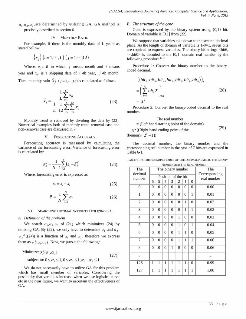
We suppose that variables take down to the second decimal place. As the length of domain of variable is 1-0=1, seven bits are required to express variables. The binary bit strings <bit6,

～,bit0> is decoded to the [0,1] domain real number by the following procedure.[21]

Procedure 1: Convert the binary number to the binary-coded decimal.

(28)

Procedure 2: Convert the binary-coded decimal to the real number.

The real number

= (Left hand starting point of the domain)

+ ((Right hand ending point of the

domain)/( ))

(29)

The decimal number, the binary number and the corresponding real number in the case of 7 bits are expressed in Table 6-1.

TABLE 6-1: CORRESPONDING TABLE OF THE DECIMAL NUMBER, THE BINARY

NUMBER AND THE REAL NUMBER

The

decimal

number

The binary number The

Corresponding

real number Position of the bit

6 5 4 3 2 1 0

0 0 0 0 0 0 0 0 0.00

1 0 0 0 0 0 0 1 0.01

2 0 0 0 0 0 1 0 0.02

3 0 0 0 0 0 1 1 0.02

4 0 0 0 0 1 0 0 0.03

5 0 0 0 0 1 0 1 0.04

6 0 0 0 0 1 1 0 0.05

7 0 0 0 0 1 1 1 0.06

8 0 0 0 1 0 0 0 0.06

… …

126 1 1 1 1 1 1 0 0.99

127 1 1 1 1 1 1 1 1.00

321 ,,

12,,1,,1 jLixij

Rxij j i

ijx i j

jx~ 12,,1j

L

i j

ij

L

i

ij

j

xL

xL

x

1

12

1

1

12

11

1

~

N

i

iN 1

22

1

1

iii xx ˆ

N

i

iN

1

1

321 ,,

1 2

2 1 2

),( 212

),( 21

2

1,10,10 2121 　　　　

X

bit

bitbitbitbitbitbitbit

i

i

i

10

6

0

20123456

2

,,,,,,

'X

127



1 variable is expressed by 7 bits, therefore 2 variables needs 14 bits. The gene structure is exhibited in Table 6-2.

Table 6-2: The gene structure

Position of the bit 13 12 11 10 9 8 7 6 5 4 3 2 1 0

0-

1

0-

1

0-

1

0-

1

0-

1

0-

1

0-

1

0-

1

0-

1

0-

1

0-

1

0-

1

0-

1

0-

1

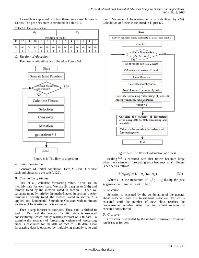
C. The flow of Algorithm

The flow of algorithm is exhibited in Figure 6-1.

Figure 6-1: The flow of algorithm

A. Initial Population

Generate M initial population. Here, 100M . Generate each individual so as to satisfy (22).

B. Calculation of Fitness

First of all, calculate forecasting value. There are 36 monthly data for each case. We use 24 data(1st to 24th) and remove trend by the method stated in section 3. Then we calculate monthly ratio by the method stated in section 4. After removing monthly trend, the method stated in section 2 is applied and Exponential Smoothing Constant with minimum variance of forecasting error is estimated.

Then 1 step forecast is executed. Thus, data is shifted to 2nd to 25th and the forecast for 26th data is executed consecutively, which finally reaches forecast of 36th data. To examine the accuracy of forecasting, variance of forecasting error is calculated for the data of 25th to 36th data. Final forecasting data is obtained by multiplying monthly ratio and

trend. Variance of forecasting error is calculated by (24). Calculation of fitness is exhibited in Figure 6-2.

Figure 6-2: The flow of calculation of fitness

Scaling [22] is executed such that fitness becomes large when the variance of forecasting error becomes small. Fitness is defined as follows

),(),( 21

2

21 Uf (30)

Where U is the maximum of ),( 212

during the past

W generation. Here, W is set to be 5.

C. Selection

Selection is executed by the combination of the general elitist selection and the tournament selection. Elitism is executed until the number of new elites reaches the predetermined number. After that, tournament selection is executed and selected.

D. Crossover

Crossover is executed by the uniform crossover. Crossover rate is set as follows.

1 2



7.0cP (31)

E. Mutation

Mutation rate is set as follows

05.0mP (32)

Mutation is executed to each bit at the probability mP ,

therefore all mutated bits in the population M becomes

14MPm.

VII. NUMERICAL EXAMPLE

A. Application to the original production data of Wheelchairs

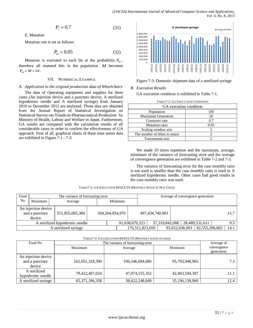
The data of Operating equipment and supplies for three cases (An injection device and a puncture device, A sterilized hypodermic needle and A sterilized syringe) from January 2010 to December 2012 are analyzed. These data are obtained from the Annual Report of Statistical Investigation on Statistical-Survey-on-Trends-in-Pharmaceutical-Production by Ministry of Health, Labour and Welfare in Japan. Furthermore, GA results are compared with the calculation results of all considerable cases in order to confirm the effectiveness of GA approach. First of all, graphical charts of these time series data are exhibited in Figure 7-1 - 7-3.

Figure 7-3: Domestic shipment data of a sterilized syringe

B. Execution Results

GA execution condition is exhibited in Table 7-1.

TABLE7-1: GA EXECUTION CONDITION

GA execution condition

Population 100

Maximum Generation 50

Crossover rate 0.7

Mutation ratio 0.05

Scaling window size 5

The number of elites to retain 2

Tournament size 2

We made 10 times repetition and the maximum, average, minimum of the variance of forecasting error and the average of convergence generation are exhibited in Table 7-2 and 7-3.

The variance of forecasting error for the case monthly ratio is not used is smaller than the case monthly ratio is used in A sterilized hypodermic needle. Other cases had good results in the case monthly ratio was used.

TABLE7-2: GA EXECUTION RESULTS (MONTHLY RATIO IS NOT USED)

Food No

The variance of forecasting error Average of convergence generation

Maximum Average Minimum

An injection device

and a puncture

device

551,855,685,384 504,204,854,970 497,434,740,003 15.7

A sterilized hypodermic needle 91,638,679,323 37,319,843,068 28,489,531,611 9.5

A sterilized syringe 176,511,823,650 93,652,636,003 82,555,206,063 14.1

TABLE7-3: GA EXECUTION RESULTS (MONTHLY RATIO IS USED)

Food No The variance of forecasting error Average of convergence generation

Maximum Average Minimum

An injection device

and a puncture

device

162,051,318,390 106,546,694,680 95,793,948,965 7.3

A sterilized hypodermic needle

79,422,467,024 47,074,155,352 42,493,594,397 11.1

A sterilized syringe 65,371,396,358 38,622,248,849 35,196,139,960 12.4



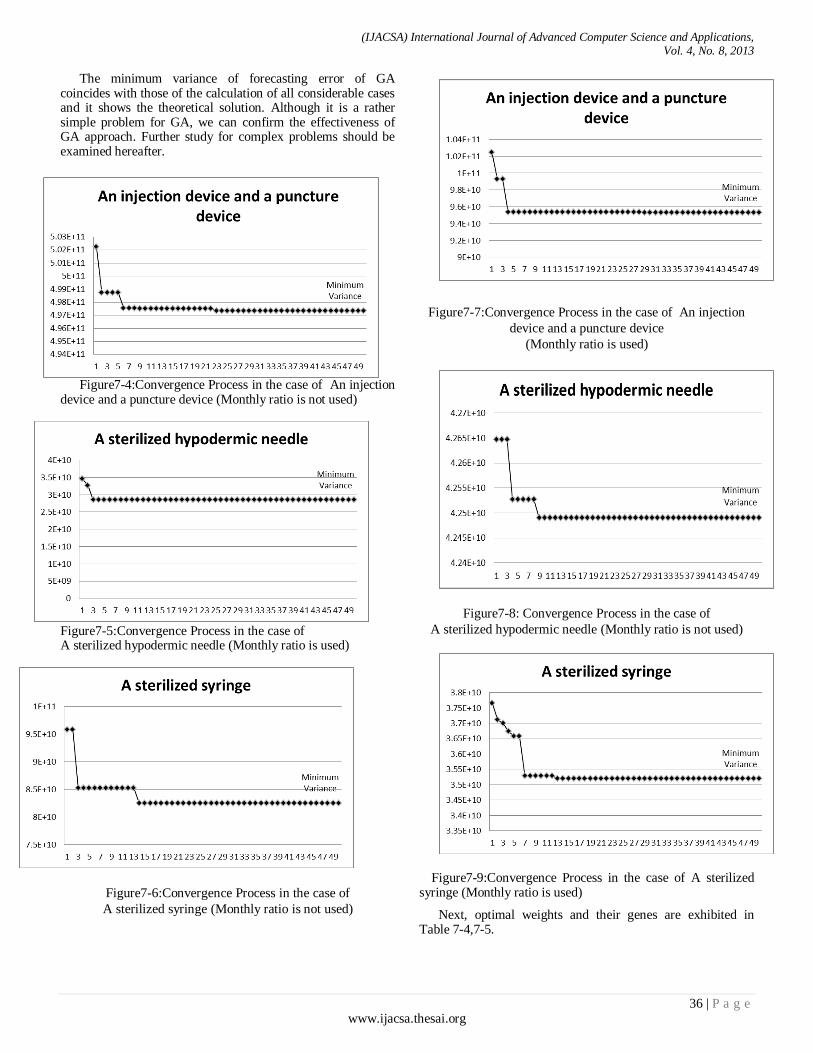
The minimum variance of forecasting error of GA coincides with those of the calculation of all considerable cases and it shows the theoretical solution. Although it is a rather simple problem for GA, we can confirm the effectiveness of GA approach. Further study for complex problems should be examined hereafter.

Figure7-4:Convergence Process in the case of An injection device and a puncture device (Monthly ratio is not used)

Figure7-5:Convergence Process in the case of A sterilized hypodermic needle (Monthly ratio is used)

Figure7-6:Convergence Process in the case of

A sterilized syringe (Monthly ratio is not used)

Figure7-7:Convergence Process in the case of An injection

device and a puncture device

(Monthly ratio is used)

Figure7-8: Convergence Process in the case of

A sterilized hypodermic needle (Monthly ratio is not used)

Figure7-9:Convergence Process in the case of A sterilized

syringe (Monthly ratio is used)

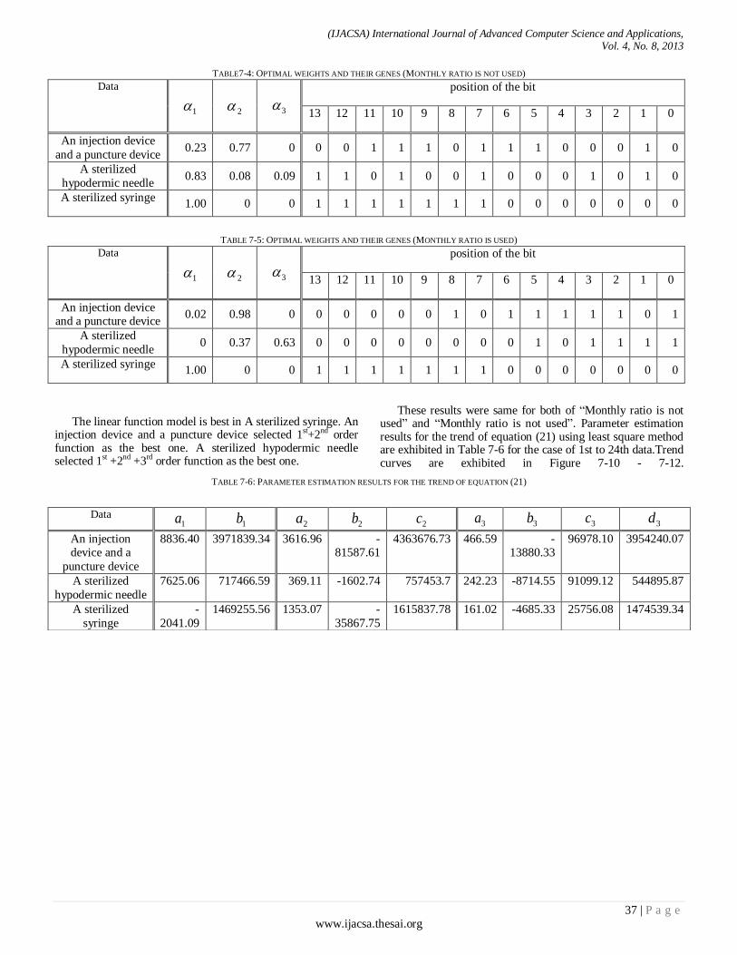
Next, optimal weights and their genes are exhibited in Table 7-4,7-5.



TABLE7-4: OPTIMAL WEIGHTS AND THEIR GENES (MONTHLY RATIO IS NOT USED)

Data

1 2 3

position of the bit

13 12 11 10 9 8 7 6 5 4 3 2 1 0

An injection device

and a puncture device 0.23 0.77 0 0 0 1 1 1 0 1 1 1 0 0 0 1 0

A sterilized

hypodermic needle 0.83 0.08 0.09 1 1 0 1 0 0 1 0 0 0 1 0 1 0

A sterilized syringe 1.00 0 0 1 1 1 1 1 1 1 0 0 0 0 0 0 0

TABLE 7-5: OPTIMAL WEIGHTS AND THEIR GENES (MONTHLY RATIO IS USED)

Data

1 2 3

position of the bit

13 12 11 10 9 8 7 6 5 4 3 2 1 0

An injection device and a puncture device

0.02 0.98 0 0 0 0 0 0 1 0 1 1 1 1 1 0 1

A sterilized

hypodermic needle 0 0.37 0.63 0 0 0 0 0 0 0 0 1 0 1 1 1 1

A sterilized syringe 1.00 0 0 1 1 1 1 1 1 1 0 0 0 0 0 0 0

The linear function model is best in A sterilized syringe. An injection device and a puncture device selected 1st+2nd order function as the best one. A sterilized hypodermic needle selected 1st +2nd +3rd order function as the best one.

These results were same for both of “Monthly ratio is not used” and “Monthly ratio is not used”. Parameter estimation results for the trend of equation (21) using least square method are exhibited in Table 7-6 for the case of 1st to 24th data.Trend curves are exhibited in Figure 7-10 - 7-12.

TABLE 7-6: PARAMETER ESTIMATION RESULTS FOR THE TREND OF EQUATION (21)

Data 1a 1b 2a 2b 2c 3a 3b 3c 3d

An injection device and a

puncture device

8836.40 3971839.34 3616.96 -81587.61

4363676.73 466.59 -13880.33

96978.10 3954240.07

A sterilized

hypodermic needle

7625.06 717466.59 369.11 -1602.74 757453.7 242.23 -8714.55 91099.12 544895.87

A sterilized

syringe

-

2041.09

1469255.56 1353.07 -

35867.75

1615837.78 161.02 -4685.33 25756.08 1474539.34



Figure7-10: Trend of An injection device and a puncture device

Figure7-11: Trend of A sterilized hypodermic needle



Figure7-12: Trend of A sterilized syringe

Calculation results of Monthly ratio for 1st to 24th data are exhibited in Table 7-7.

Table 7-7: PARAMETER ESTIMATION RESULT OF MONTHLY RATIO

Date. 1 2 3 4 5 6 7 8 9 10 11 12

An injection device and

a puncture device 0.901 1.038 0.960 1.015 0.868 0.997 1.039 0.968 0.999 0.995 1.063 1.158

A sterilized hypodermic

needle 1.146 0.900 0.735 1.072 0.866 1.033 1.094 0.984 0.993 0.993 0.986 1.198

A sterilized syringe 0.941 1.076 0.887 0.95 0.84 1.02 1.078 0.883 1.004 1.088 1.137 1.071

Estimation result of the smoothing constant of minimum

variance for the 1st to 24th data are exhibited in Table 7-8, 7-9.

Forecasting results are exhibited in Table 7-13 - 7-15.

Table 7-8:SMOOTHING CONSTANT OF MINIMUM VARIANCE OF EQUATION (17)

(MONTHLY RATIO IS NOT USED)

Date ρ1 α


puncture device -0.147880 0.848737


needle -0.342724 0.603356

A sterilized syringe -0.499464 0.045270

Table 7-9: SMOOTHING CONSTANT OF MINIMUM VARIANCE OF EQUATION

(17) (MONTHLY RATIO IS USED)

Date, ρ1 α


puncture device -0.293350 0.675822


needle -0.067694 0.931993

A sterilized syringe -0.171119 0.823554



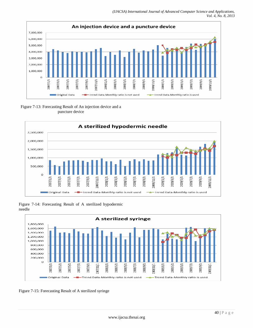
Figure 7-13: Forecasting Result of An injection device and a

puncture device

Figure 7-14: Forecasting Result of A sterilized hypodermic

needle

Figure 7-15: Forecasting Result of A sterilized syringe



C. Remarks

The linear function model in the case Monthly ratio was used was best for A sterilized syringe case. 1st+2nd function model in the case Monthly ratio was used was best for An injection device and a puncture device case. 1st+2nd +3rd function model in the case Monthly ratio was not used was best for A sterilized hypodermic needle case.

The minimum variance of forecasting error of GA coincides with those of the calculation of all considerable cases and it shows the theoretical solution. Although it is a rather simple problem for GA, we can confirm the effectiveness of GA approach. Further study for complex problems should be examined hereafter.

VIII. CONCLUSION

Focusing on the idea that the equation of exponential smoothing method(ESM) was equivalent to (1,1) order ARMA model equation, a new method of estimation of smoothing constant in exponential smoothing method was proposed before by us which satisfied minimum variance of forecasting error. Generally, smoothing constant was selected arbitrarily. But in this paper, we utilized above stated theoretical solution. Firstly, we made estimation of ARMA model parameter and then estimated smoothing constants. Thus theoretical solution was derived in a simple way and it might be utilized in various fields.

Furthermore, combining the trend removal method with this method, we aimed to improve forecasting accuracy. An approach to this method was executed in the following method. Trend removal by a linear function was applied to the data of Operating equipment and supplies for three cases (An injection device and a puncture device, A sterilized hypodermic needle and A sterilized syringe). The combination of linear and non-linear function was also introduced in trend removal. Genetic Algorithm was utilized to search the optimal weight for the weighting parameters of linear and non-linear function. For the comparison, monthly trend was removed after that. Theoretical solution of smoothing constant of ESM was calculated for both of the monthly trend removing data and the non monthly trend removing data. Then forecasting was executed on these data. The new method shows that it is useful for the time series that has various trend characteristics. The effectiveness of this method should be examined in various cases.

REFERENCES

[1] Box Jenkins. (1994) Time Series Analysis Third Edition，Prentice Hall.

[2] R.G. Brown. (1963) Smoothing, Forecasting and Prediction of Discrete

–Time Series, Prentice Hall.

[3] Hidekatsu Tokumaru et al. (1982) Analysis and Measurement –Theory

and Application of Random data Handling, Baifukan Publishing.

[4] Kengo Kobayashi. (1992) Sales Forecasting for Budgeting, Chuokeizai-

Sha Publishing.

[5] Peter R.Winters. (1984) Forecasting Sales by Exponentially Weighted Moving Averages, Management Science，Vol6，No.3, pp. 324-343.

[6] Katsuro Maeda. (1984) Smoothing Constant of Exponential Smoothing

Method, Seikei University Report Faculty of Engineering, No.38, pp. 2477-2484.

[7] M.West and P.J.Harrison. (1989) Baysian Forecasting and Dynamic

Models，Springer-Verlag，New York.

[8] Steinar Ekern. (1982) Adaptive Exponential Smoothing Revisited，Journal of the Operational Research Society, Vol．32 pp．775-782.

[9] F.R.Johnston. (1993) Exponentially Weighted Moving Average

(EWMA) with Irregular Updating Periods, Journal of the Operational Research Society，Vol.44，No.7 pp．711-716.

[10] Spyros Makridakis and Robeat L.Winkler. (1983) Averages of Forecasts；Some Empirical Results，Management Science，Vol.29,

No.9, pp. 987-996.

[11] Naohiro Ishii et al. (1991) Bilateral Exponential Smoothing of Time Series, Int.J.System Sci., Vol.12, No.8, pp. 997-988.

[12] Kazuhiro Takeyasu and Keiko Nagata.(2010) Estimation of Smoothing

Constant of Minimum Variance with Optimal Parameters of Weight, International Journal of Computational Science Vol.4,No.5, pp. 411-425.

[13] Kazuhiro Takeyasu, Keiko Nagata, Yuki Higuchi. (2009) Estimation of

Smoothing Constant of Minimum Variance And Its Application to Shipping Data With Trend Removal Method, Industrial Engineering ＆

Management Systems (IEMS),Vol.8,No.4, pp.257-263,

[14] Kazuhiro Takeyasu, Keiko Nagata, Yui Nishisako. (2010) A Hybrid Method to Improve Forecasting Accuracy Utilizing Genetic Algorithm

And Its Application to Industrial Data, NCSP'10, Honolulu,Hawaii,USA

[15] Kazuhiro Takeyasu, Keiko Nagata, Kana Takagi. (2010) Estimation of Smoothing Constant of Minimum Variance with Optimal Parameters of

Weight, NCSP'10, Honolulu,Hawaii,USA

[16] Kazuhiro Takeyasu, Keiko Nagata, Tomoka Kuwahara. (2010)

Estimation of Smoothing Constant of Minimum Variance Searching Optimal Parameters of Weight, NCSP'10, Honolulu,Hawaii,USA

[17] Kazuhiro Takeyasu, Keiko Nagata, Mai Ito, Yuki Higuchi (2010). A

Hybrid Method to Improve Forecasting Accuracy Utilizing Genetic Algorithm, The 11th APEIMS, Melaka, Malaysia

[18] Kazuhiro Takeyasu, Keiko Nagata, Kaori Matsumura. (2011) Estimation

of Smoothing Constant of Minimum Variance and Its Application to Sales Data, JAIMS, Honolulu, Hawaii, USA

[19] Hiromasa Takeyasu, Yuki Higuchi, Kazuhiro Takeyasu. (2012) A

Hybrid Method to Improve Forecasting Accuracy in the Case of Bread, International Journal of Information and Communication Technology

Research, Vol.2 , No.11, pp.804～812.

[20] Kazuhiro Takeyasu and Kazuko Nagao.(2008) Estimation of Smoothing Constant of Minimum Variance and its Application to Industrial Data,

Industrial Engineering and Management Systems, vol.7, no. 1, pp. 44-50.

[21] Masatosi Sakawa. Masahiro Tanaka. (1995 ） Genetic Algorithm 、Asakura Pulishing Co., Ltd.

[22] Hitoshi Iba.（2002）Genetic Algorithm、Igaku Publishing.

a hybrid method to improve forecasting accuracy utilizing ... · abstract—in industries, how to...

Documents