A Hub-Based Labeling Algorithm forShortest Paths on Road Networks

Ittai Abraham Daniel Delling Andrew V. Goldberg Renato F. WerneckMicrosoft Research Silicon Valley, 1065 La Avenida, Mountain View, CA 94043, USA

December 2010

Technical ReportMSR-TR-2010-165

Abraham et al. [SODA 2010] have recently presented a theoretical analysis of severalpractical point-to-point shortest path algorithms based on modeling road networksas graphs with low highway dimension. Among the methods they analyzed, the onewith the best time bounds is the labeling algorithm. Their results suggest that thealgorithm is interesting from a theoretical viewpoint, but leave open the existence ofa practical implementation. This paper presents such an implementation and showsexperimental evidence that it is actually faster than the fastest method previouslystudied.

Microsoft ResearchMicrosoft CorporationOne Microsoft Way

Redmond, WA 98052http://www.research.microsoft.com

1 Introduction

Motivated by computing driving directions, the problem of finding point-to-point shortest pathsin road networks has received significant attention in recent years. Even though Dijkstra’s al-gorithm [8, 14] solves the problem in almost linear time [17], applications to continent-size roadnetworks require faster algorithms. Preprocessing makes sublinear-time algorithms possible.

There are too many preprocessing-based methods too describe in full—we refer the readerto [12] for a comprehensive overview. We present here only some highlights with the algorithmsthat are relevant to our study. Arc flags [23, 21] and landmark-based A∗ search [18] reduce thesearch space by directing the search towards the goal. Highway hierarchies [26, 27] and reach [20,19] use hierarchical properties of road networks to sparsify the search. One of the key ingredients ofefficient implementations of these methods is the notion of a shortcut (introduced by Sanders andSchultes [26]), which is a new arc representing a shortest path between its endpoints. Shortcutsby themselves became the basis of contraction hierarchies (CH) [16], an elegant algorithm thatmotivated much follow-up work. Another method is transit node routing (TNR) [3, 4], whichis based on the observation that there is a small set of vertices that cover all sufficiently longshortest paths out of any region of a road network. This allows long-range queries to be reducedto a small number of table look-ups. The most efficient implementation of TNR uses CH duringthe preprocessing stage and to handle local queries [16]. One can combine goal-direction withhierarchical methods or TNR [19, 6, 5]. In particular, the fastest previously known point-to-pointshortest path algorithm [6] combines elements from TNR (using CH) and arc flags. It is six ordersof magnitude faster than Dijkstra’s algorithm for random (long-range) queries.

Although these algorithms have been shown to work well in practice, a theoretical analysis hasbeen given only recently, in a paper by Abraham et al. [1]. It is based on modeling road networksas graphs with low highway dimension. The method with the best time bounds, presented byAbraham et al. as a variant of TNR, is actually a labeling algorithm. Labeling algorithms havebeen studied before in the distributed computing literature [15, 30]. In particular, [15] givesupper and lower bounds on label sizes for general graphs, trees, planar graphs, and boundeddegree graphs.

Like most speedup techniques on road networks, the labeling algorithm works in two stages.The preprocessing stage computes for each vertex v a forward label Lf (v) and a reverse labelLr(v). The forward label consists of a set of vertices w, together with their respective distancesdist(v, w) from v. Similarly, the reverse label consists of a set of vertices u, each with its distancedist(u, v) to v. The labels have the following cover property: For every pair of distinct verticess and t, Lf (s) ∩ Lr(t) contains a vertex u on a shortest path from s to t. To emphasize that alabeling has the cover property, we call a labeling valid.

The query stage of the labeling algorithm is quite simple, given the cover property. Givens and t, find the vertex u ∈ Lf (s) ∩ Lr(t) that minimizes dist(s, u) + dist(u, t) and return thecorresponding path. One can think of a label for a vertex v as a set of hubs to which v has adirect connection. The cover property ensures that any two vertices share at least one hub on theshortest path between them.

The results of Abraham et al. [1] suggest that the labeling algorithm is interesting froma theoretical viewpoint, but leave open the existence of a practical implementation. In fact,as described in their paper, the algorithm appears impractical. First, preprocessing, althoughpolynomial-time, is too slow for continent-size networks. Second, the worst-case bound on the

1

memory overhead per vertex is also too high for a practical implementation on such networks.In this paper we give a practical implementation of the labeling algorithm. Our preprocessing

algorithm uses the contraction hierarchies (CH) algorithm by Geisberger et al. [16], which wereview in Section 3, and augments it with other techniques. We call our implementation HL(Hub-based Labeling algorithm). Our contributions are as follows:

• We observe that the sets of vertices visited by the forward and reverse searches of hierarchicaland reach-based algorithms contain the corresponding labels. More precisely, visited verticeswith exact distance values form valid labels. Similar observations have appeared for graphsof bounded tree-width [15] and for road networks [22] in an implicit manner; we make itexplicit and take advantage of it.

• We use the above observation to implement a labeling algorithm by pruning the CH searchspace. We observe that this produces labels that are small enough to store in main memoryeven for continental-sized road networks.

• We show how to use ideas from “theoretical” preprocessing algorithms [1] to improve thequality of the fast heuristic CH preprocessing, leading to even smaller labels.

• We show how to implement efficiently the preprocessing and query stages of HL, includingsimple but effective techniques to accelerate long-range queries.

• We describe a label compression technique that significantly reduces the space requirementsof the algorithm.

• We present experiments showing trade-offs of our implementation and comparing it to thefastest previous codes.

The results show that the labeling algorithm is not only theoretically efficient, but actually prac-tical. In fact, when optimized for speed, for random queries our algorithm is about as fast as fiverandom accesses to main memory.

The main contribution of this paper is to show that HL is practical and should be consideredfor real-life applications. An added bonus is that HL is currently the fastest algorithm for theproblem. While simpler than the previous state of the art, the combination of TNR and arc flags(TNR+AF) discussed above, HL is faster by a factor of more than three for long-range queries(although HL memory usage is higher by a small constant factor). For short-range queries, theperformance difference between HL and TNR+AF is even greater—an order of magnitude. Byapplying our compression techniques, HL has roughly the same memory footprint as TNR+AF,and still outperforms it.

This paper is organized as follows. Section 2 gives basic definitions and reviews Dijkstra’salgorithm. Section 3 gives a quick summary of the CH algorithm. Section 4 presents the basicversion of our labeling algorithm. Section 5 shows how it can be improved, leading to an evenmore practical algorithm. We evaluate the algorithm experimentally in Section 6, and concludein Section 7.

2

2 Preliminaries

The input to the preprocessing stage of a shortest path algorithm is a graph G = (V,A) withlength `(a) > 0 for every arc a. We denote the number of vertices in G by n. The length of anypath P in G is the sum of the lengths of its arcs. The distance between vertices v and w, denotedby dist(v, w), is the length of the shortest path between them. The query phase of the shortestpath algorithm takes as input a source s and a target t, and returns dist(s, t).

Dijkstra’s algorithm [14, 8] is the best-known method for computing shortest paths in oursetting. It is an efficient implementation of the scanning method for graphs with non-negative arclengths (see e.g. [29]). For every vertex v, it maintains the length d(v) of the shortest path fromthe source s to v found so far, as well as the predecessor p(v) of v on the path. Initially d(s) = 0,d(v) = ∞ for all other vertices, and p(v) = null for all v.

Dijkstra’s algorithm maintains a priority queue of unscanned vertices with finite d values, thevalues serving as keys. At each step, the algorithm extracts a vertex v with minimum value fromthe queue and scans it: for each arc (v, w) ∈ A, if d(v)+`(v, w) < d(w) it sets d(w) = d(v)+`(v, w)and p(v) = w. The algorithm terminates when the target t is extracted, without scanning t.

3 Contraction Hierarchies

We now discuss contraction hierarchies (CH) [16], an acceleration technique that, on road net-works, can find exact point-to-point shortest paths orders of magnitude faster than Dijkstra’salgorithm.

Most state-of-the-art shortest-path algorithms, including the CH algorithm, depend cruciallyon a very simple notion: shortcuts [26]. Given two vertices u, v ∈ V , a shortcut (or shortcut arc)is a new arc (u, v) with length dist(u, v), the original distance in G between u and v. The shortcutoperation deletes (temporarily) a vertex v from the graph and adds shortcut arcs between itsneighbors to maintain the shortest path information. More precisely, for any neighbors u, w suchthat (u, v) · (v, w) is the only shortest path between u and w, we add the shortcut (u, w) with`(u, w) = `(u, v) + `(v, w).

Given the notion of shortcuts, CH preprocessing is simple: define a total order among thevertices and shortcut them sequentially in this order, until a single vertex remains. The outputof this routine is a graph G+ = (V,A∪A+) (where A+ is the set of shortcut arcs created), as wellas the vertex order itself. We denote the position of a vertex v in the ordering by rank(v). DefineG↑ = (V,A↑) by A↑ = {(v, w) ∈ A∪A+ : rank(v) < rank(w)}. Similarly, A↓ = {(v, w) ∈ A∪A+ :rank(v) > rank(w)} and G↓ = (V,A ∪A↓).

During an s–t query, the algorithm performs a forward search from s and a reverse searchfrom t. The forward CH search consists of running Dijkstra’s algorithm from s in G↑, stoppingwhen there are no more vertices to scan. Similarly, the reverse CH search consists of runninga reverse version of Dijkstra’s algorithm from t in G↓. With these searches, the CH algorithmcomputes upper bound estimates ds(v) and dt(v) on distances from s to v and from v to t for everyv ∈ V . For some vertices, these estimates may be greater than the actual distances; in fact, manyvertices are not visited by the search and (implicitly) have infinite estimates. However, as shownby Geisberger et al. [16], the maximum-rank vertex u on the s–t shortest path is guaranteed tobe visited, v = u will minimize ds(v)+dt(v), and this will be the length of the shortest path froms to t. The path itself can be obtained from the concatenation of the s–u and u–t paths.

3

Note that queries are correct regardless of the contraction order, but query complexity andthe number of shortcuts added may vary greatly from one permutation to the next. The bestresults reported in [16] are obtained by on-line heuristics that select the next vertex to shortcutbased on its current degree and the number of new arcs added to the graph, among other factors.

We use a slightly different priority function for ordering vertices [9]. The priority of a vertex uis given by 2 ·ED(u)+CN (u)+H(u)+5 ·L(u), where ED(u) is the difference between the numberof arcs added and removed (if u were shortcut), CN(u) is the number of previously contractedneighbors, H(u) is the total number of underlying arcs represented by all shortcuts added, andL(u) is the level u would be assigned to.

The level of a vertex u, denoted by level(u), is defined as follows. If all neighbors of u inG+ have higher rank than u, level(u) = 0. Otherwise, level(u) = level(v) + 1, where v is thehighest-level vertex among all lower-ranked neighbors of u.

4 Basic HL

In this section, we first review the theoretically justified labeling algorithm of Abraham et al. [1],then we describe our practical implementation.

4.1 The Theoretical Algorithm

The preprocessing of the theoretical labeling algorithm [1] is based on shortest path covers (SPCs).Intuitively, an (r, k)-shortest path cover S is a set of vertices that (1) hits every shortest path oflength between r and 2r and (2) is sparse, in the sense that every ball of radius 2r contains atmost k elements from S. Computing such covers is probably NP-hard, but the authors suggest agreedy algorithm to obtain an O(log n) approximation in polynomial time.

More precisely, the assumptions of [1] imply that for a fixed parameter h, (r, h)-SPCs exist forall r, and the greedy algorithm computes an O(r, O(h log n))-SPC. The parameter h, the highwaydimension of the graph, is believed to be small for road networks.

As suggested by Abraham et al., preprocessing for the labeling algorithm uses the greedyalgorithm to compute SPCs Ci for r = 2i, 0 ≤ i ≤ log D, where D is the diameter of thegraph. The paper proves that the following labeling is valid: For each v, take the union over iof Ci intersected with the ball of radius 2 · 2i around v. Note that the size of the label of v isO(k log n log D).

As stated, the algorithm is not practical. First, the greedy algorithm for computing SPCsrequires computing all-pairs shortest paths many times over, yielding preprocessing times of sev-eral months for continent-size networks. Second, the theoretical bound on the label size couldbe well into the thousands in practice, which would lead to unrealistic space requirements anduncompetitive query times.

4.2 A Practical Implementation

Before explaining our new practical implementation of the labeling algorithm, we need the notionof a superlabel. Given a vertex v, it is defined similarly to a label, except for the fact that adistance d(v, w) stored within the label need not equal the real distance dist(v, w). We onlyenforce d(v, w) ≥ dist(v, w). For simplicity, we refer to superlabels as labels except when we want

4

to emphasize that we are dealing with superlabels. When we want to stress that we deal withlabels according to the original definition, we will refer to them as strict labels. We also use thesame notation, Lf (v) and Lr(v), for superlabels. The cover property for superlabels is defined asfollows: For every pair of distinct vertices s and t, Lf (s) ∩ Lr(t) contains a vertex u such that uis on a shortest path from s to t, d(s, u) = dist(s, u), and d(u, t) = dist(u, t). It is obvious thatthe query algorithm remains correct when superlabels are given.

The idea of our new implementation of the labeling algorithm is as follows. Given s and t,consider the sets of vertices visited by the forward CH search from s and the reverse CH searchfrom t. CH works because the intersection of these sets contains the maximum-rank vertex u onthe shortest s–t path. Therefore, we can obtain a valid superlabeling if we define, for every v,Lf (v) and Lr(v) to be the sets of vertices visited by the forward and reverse CH searches fromv. (For undirected—i.e., symmetric—graphs, one label would be sufficient.) This is similar tothe many-to-many algorithm of Knopp et al. [22], which during queries computes and stores thesets of vertices visited by the reverse search from the destinations, along with the distance labels.Note that the many-to-many algorithm implicitly uses the fact that these sets form superlabels.

On the road network of Western Europe (used for most of our experiments), the average sizeof the labels computed this way is about 500. For a practical algorithm, we would like to havesmaller labels. Note that if we have a forward superlabel Lf (v), we can prune it by deleting from itvertices w with d(v, w) > dist(v, w). We can prune Lr(v) similarly. If before pruning u is a vertexin Lf (s)∩Lr(t) with d(s, u) = dist(s, u) and d(u, t) = dist(u, t), u will not be pruned. Therefore.superlabels remain valid after pruning. Partial pruning and complete pruning delete some and allvertices that can be pruned, respectively. On road networks, complete pruning reduces the labelsize significantly (about 80% on the benchmark instance).

We now consider a simple way of representing a label so as to allow efficient queries. Weidentify a vertex i with its (integer) ID. We describe the Lf labels; the Lr labels are symmetric.The label Lf (v) is represented as the concatenation of three elements:

• Nv is an integer representing the number of vertices in the label.

• Iv is a zero-based array containing the IDs of all vertices in the label in ascending order.

• Dv is an array containing the distances from v to the vertices in its label (in the same orderas Iv): Dv[i] = dist(v, Iv[i]).

With this representation, the query algorithm is straightforward. Given s and t, it must pick,among all vertices w ∈ Lf (s) ∩ Lr(t), the one minimizing dist(s, w) + dist(w, t) = ds(w) + dt(w).The fact that the Iv arrays are sorted allows this computation to be performed in linear time,with a single sweep through the labels, similar to mergesort. We maintain array indices is and it(initially zero) and a tentative distance µ (initially infinite). At each step we compare Is[is] andIt[it]. If these IDs are equal, we found a new w in the intersection of the labels, so we compute anew tentative distance Ds[is]+Dt[it], update µ if necessary, then increment both is and it. If theIDs differ, we increment either is (if Is[is] < It[it]) or it (if Is[is] > It[it]). We stop when eitheris = Ns or it = Nt, and return µ.

A crucial aspect of this algorithm is that each array is accessed sequentially. Good localityreduces the number of cache misses, which are the bottleneck of our algorithm.

For added efficiency, in practice we actually use pointer arithmetic (instead of maintainingindices) and use sentinels to detect when a particular array has been traversed in full. We discuss

5

further improvements to our basic algorithm in the next section.

5 Improvements

As we have seen, our basic preprocessing and query algorithms are simple, given an implementationof CH. In this section we describe improvements that speed up preprocessing and queries, or reducespace overhead of the algorithm.

When discussing algorithmic details, one should keep in mind that our fastest query imple-mentation is less than five times slower than a random memory access, as Section 6 will show. Toachieve this, we need to consider low-level implementation details carefully. Locality is particularlyimportant, since each additional cache miss results in noticeable performance penalty.

5.1 Fast Preprocessing

We now describe a detailed implementation of the preprocessing algorithm outlined in Section 4,together with some improvements. Recall that we must compute forward and reverse labels foreach vertex v.

Our algorithm works as follows. For every v ∈ V , start with Lf (v) = ∅. Run the forward CHsearch from v and add to L(v) all vertices w with ds(w) = dist(v, w). Compute Lr(v) similarlyusing the reverse CH search. Since a CH search is very fast (a fraction of a millisecond on WesternEurope), doing the required 2n searches is practical.

However, while performing a search from v, for each vertex w visited we must check if itsdistance label d(w) matches the actual distance dist(s, w). We can use any efficient point-to-pointshortest path algorithm for these check queries. In fact, as Section 5.2 will explain, one canbootstrap and use HL itself.

Even though HL is fast, it is not free. Therefore, we also use a fast heuristic modificationto the CH search to identify most vertices with incorrect distance labels, thus avoiding someunnecessary check queries. The heuristic is similar to the stall-on-demand procedure used by CHand related algorithms [28]. We describe it for the forward search; the reverse search can be dealtwith similarly. Suppose we are performing a forward CH search from v and we are about to scanw, which has distance label d(w). The modification examines all incoming arcs (u, w) ∈ A↓. Ifd(w) > d(u) + `(u, w), the distance label of w is provably incorrect. Therefore, we can safelyremove w from the label, and we do not scan outgoing arcs from it. It is easy to see that thefollowing holds:

Lemma 5.1 Every vertex visited by the original forward CH search and assigned a correct dis-tance label is visited by the modified CH search and assigned a correct distance label.

We can generalize this approach for better pruning as follows. When scanning a vertex w withdistance d(w) during a forward CH search, we perform a graph search from w in A↓, limited todepth h. If we find a vertex u with d(u)+d∗(u, w) < d(w), where d∗(u, w) is the distance betweenu and w with respect to the graph search, we remove w from the label and do not scan outgoingarcs from w. We call this approach h-hop heuristic label pruning, where h is a user-definedparameter.

Our experiments show that only a small fraction of the vertices that remain (after the h-hopheuristic is applied) have incorrect labels, even with h = 1. This means one could skip the check

6

queries altogether to save preprocessing time, and use these partially pruned labels for queries.Still, for optimum query performance, we do perform the checks during preprocessing to obtainstrict labels in most of our experiments.

Note that the labels of different vertices can be computed completely independently. Therefore,parallelizing the label computation is straightforward.

5.2 Bootstrapping

The partially pruned label preprocessing algorithm finds most vertices that can be pruned, butit may miss some. One can prune further to obtain strict labels using a point-to-point queryalgorithm. In this section we describe how to bootstrap HL, i.e., use HL itself as the queryalgorithm. In addition to eliminating the need to implement another algorithm, this is attractivebecause HL is one of the fastest point-to-point shortest path algorithms.

A simple way to do bootstrapping is as follows. First, compute partially pruned labels. Then,for every label Lf (v) (Lr(v)), iterate through the vertices w in the label and use point-to-pointqueries to check if d(w) = dist(v, w) (d(w) = dist(w, v)). It the test fails, delete w from the label.

One can do more efficient bootstrapping by pruning the labels as they are computed, elim-inating the need to store bigger intermediate labels except for the current vertex. To do this,we compute the labels for vertices in descending level order. We describe how to compute theforward labels; the reverse case is similar. Suppose we have just computed the partially prunedlabel Lf (v). We know that d(v) = 0 and that all other vertices w in Lf (v) have higher level thanv, which means Lr(w) must have already been computed. We can therefore compute dist(v, w)using Lf (v) and Lr(w), removing w from Lf (v) if d(w) > dist(v, w).

If we use bootstrapping during preprocessing, we have to be more careful for a parallel im-plementation. Computing the label of a vertex v in level i requires access to labels of verticesin levels higher than i. We can process vertices of the same level in parallel, but we have tosynchronize the procedure after each level. Fortunately, the number of levels is small (about 150)on road networks. More importantly, most of the vertices are in the lowest five levels [9].

5.3 Label Ordering

Our preprocessing is CH-based and uses CH ordering of vertices. Once the labels are computed,however, we can reorder vertices (i.e., assign them new IDs) to speed up queries. We call thenewly assigned ID of a vertex its internal ID. Our experiments show that certain label orderingsyield better query times and compression rates.

Besides keeping the original input order, we also considered assigning new IDs in ascending ordescending level order (keeping the input order within each level). Moreover, we tested using theCH-rank as internal ID, as well as the inverted CH-rank. Interestingly, as we shall see in Section 6,we obtained the best results by keeping the input order for all but the topmost (highest-ranked)k vertices, which are assigned internal IDs from 0 to k − 1. We considered two variants of thismethod, depending on how IDs are assigned among the top k vertices. In the top k input order,their relative order is the same as in the input; in top k level order, these vertices are sorted bylevel.

One optimization we apply to all label orderings is to assign ID |V | to the most importantvertex. Since it is in every label of the graph (assuming the graph is strongly connected, which

7

we do), this vertex then acts as a sentinel during our sweep through the labels, thus simplifyingour termination checks.

5.4 Shortest Path Covers

As already mentioned, computing exact SPCs (or even approximations) is not practical forcontinent-size networks. However, variants of the greedy algorithm can be applied to the smallercontracted graph towards the end of CH preprocessing. In this section, we show how to do this.As we shall see in Section 6, this leads to a better CH vertex ordering and smaller labels.

CH tends to contract the least important vertices (those on few shortest paths) first, and themore important vertices (those on more shortest paths) later. The heuristic used to choose thenext vertex to contract appears to work well at the beginning of the algorithm, when choosingunimportant vertices. However, we observed that it works poorly near the end of preprocessing,when it must order important vertices relative to one another.

We now propose an algorithm that uses shortest path covers to improve the ordering ofimportant vertices. We modify our preprocessing algorithm as follows. We start by running theCH preprocessing with our original selection rule. Instead of running it to completion, however,we pause it when there are only t vertices left (a reasonable number is t = 10 000). Let Gt be thegraph at this point; it is an overlay of the original graph, i.e., it preserves the distances betweenthe remaining vertices.

In a second step, we run a greedy algorithm to find a set C of good “cover” vertices, i.e.,vertices that cover a large fraction of all shortest paths of G′, with |C| < t (we use |C| betweent/20 and t/10 in our experiments). Starting with C = ∅, at each step we add to C the vertex vthat hits the most uncovered (by C) shortest paths in Gt.

Once C has been computed, we continue the CH preprocessing, but forbid the contraction ofthe vertices in C until they are the only ones left. This guarantees that the top |C| vertices of thehierarchy will be exactly the ones in C, which are then contracted in reverse greedy order (i.e.,the first vertex found by the greedy algorithm is the last one remaining).

Greedy Cover Algorithm. We now describe the greedy algorithm mentioned above in moredetail. Let C be the (initially empty) set we are building, and suppose we need to compute thenext vertex to add to it. We do so by keeping a counter h(v) for each vertex v 6∈ C. Initiallyset to zero, this counter will eventually contain the number of uncovered shortest paths that arehit by v. We grow a shortest path tree Tr from each root r ∈ Gt. Let h(r, v) be the number ofshortest paths starting at r that are hit by v but not by C; the summation of h(r, v) over all ris h(v).

To compute h(r, v), remove from Tr all vertices already in C, together with their descendants;the paths from r to any of these vertices are already hit by C. Then traverse the resulting tree T ′

r

in bottom-up fashion. If v is a leaf of T ′r, set h(r, v) = 1; otherwise, set h(r, v) to the sum of the

h(r, u) values of its children u in the tree, plus one (to account for the path from r to v itself).As stated, the algorithm requires computing t full shortest path trees to insert each new vertex

in C. We can accelerate this process by stopping the growth of the tree as soon as all of its labeledvertices are on paths already hit by C. This does not help much while C is relatively small (thereis always an uncovered branch), but it becomes very effective as C increases in size. Still, therunning time in the worst case is O(Ct2 log t), assuming the graph has constant average degree.

8

However, we expect a significant boost in performance by computing shortest path trees withPHAST [9].

5.5 Label Compression

In this section we show how the labels can be compressed, reducing the memory consumptionof HL. We consider two independent techniques: using fewer bits to represent small IDs in eachlabel, and sharing common parts among different labels. We discuss each in turn.

5.5.1 Compressing Small IDs

The first compression technique is quite simple. Normally, we represent vertex IDs and distancesas (separate) 32-bit integers. To compress the label, we represent each of the first 256 vertices asa single 32-bit word, with 8 bits allocated to the ID and 24 bits to the distance, which is enoughfor the instances tested. Of course, one could generalize this scheme by splitting each word intob bits for IDs and ω − b bits for distances, where ω is the word size.

This 8/24 compression technique changes the representation of only 256 out of millions ofvertices. To take full advantage of this method, we must reorder vertices so that the mostimportant vertices (which tend to be in most labels) are the ones with the lowest IDs. For thiscompression scheme, a top 256 input or level ordering is most suitable.

This compression scheme is simple and adds little overhead to queries; in fact, they actuallyget faster because of better locality.

5.5.2 Compressing Common Prefixes

We now propose a different compression technique. For it to be effective, we must reorder verticesso that the important ones are assigned the very lowest IDs. For concreteness, assume we reordervertices in descending level order. For two nearby vertices in a road network, their forward (orreverse) CH trees are different near the root but are often the same when sufficiently away fromthe root. Furthermore, the vertices away from the root are the high-level (“important”) ones. Byreordering vertices in descending level order, the labels of nearby vertices will often share longcommon prefixes, with the same sets of vertices.

The intuition for our compression scheme is to compute a dictionary of the common labelprefixes and reuse them. One complication is that, even when two labels have prefixes with theexact same vertices, the corresponding distances are, in general, different. We overcome this issueby decomposing each dictionary prefix into a forest and storing distances relative to the roots.

We now describe this k-prefix compression method in detail. We explain how forward labelscan be compressed; the reverse case is symmetric. First, for each label Lf (v) we do the following.Let Pk(v) be the prefix of the label, consisting of those vertices whose internal ID is lower thank. Let Sk(v) be the suffix of the label, consisting only of the vertices whose internal ID is at leastk. In other words, the vertices in the prefix are those among the k most important in the graph;the others are in the suffix. The parameter k is the prefix threshold.

Consider the forward CH search tree T from v. The subgraph of T induced by Sk(v) eitheris empty or forms a tree containing v; the subgraph induced by Pk(v) is a forest. Consider thisforest. First suppose that Sk(v) is non-empty. For each tree Ti of the forest, let b(Ti) (the baseof Ti) denote the parent of Ti’s root. By extension, the base of a vertex w ∈ Pk(v), denoted by

9

b(w), is defined as b(Ti), if w ∈ Ti. Note that b(w) ∈ Sk(v) by definition. In the special case inwhich Sk(v) is empty (the complete tree T is in Pk(v)), we define b(v) = v.

For each w in Pk(v), we store the distance (in the tree) between b(w) and w; we denote it byδ(w). We also store b(w) itself, as the position π(w) of b(w) in Sk(v) (to save space).

Altogether, each prefix consists of a list of triples (w, δ(w), π(w)). We consider two prefixesto be equal if they consist of the exact same triples, and different if at least one triple does notmatch. We build a dictionary consisting of all distinct prefixes, which are stored sequentially inan array.

To represent a forward label Lf (v), we combine three elements: its prefix Pk(v) (representedas a reference to its position in the dictionary), the number of vertices in the prefix, and the suffixSk(v) (represented as before). Note that we do not use 8/24 compression to represent the top 256vertices.

During a query from v, suppose w is in Pk(v). Note that dist(v, w) = dist(v, b(w)) +dist(b(w), w). We can compute the distance in constant time: we precomputed dist(b(w), w) =δ(w) and we know the position π(w) of b(w) in Sk(v), where dist(v, b(w)) is stored explicitly.

5.5.3 Flexible Prefix Compression

The main drawback of the k-prefix compression is that we must use the same prefix thresholdfor all labels, even though some labels may share longer prefixes than others. In this section weshow how to extend k-prefix approach to exploit this. In the flexible prefix compression scheme,we allow each label L to be split arbitrarily into a suffix and a prefix (there are |L| ways to doso, if |L| is the number of entries in the label). As before, common prefixes are represented onlyonce and shared among labels.

Our goal is to minimize the total space consumption, considering the sizes of all (exactly n)suffixes and all (at most n) prefixes we actually keep. Obviously, there is an optimum way ofsplitting each label so as to minimize this value, but it is unclear how it can be found efficiently.Instead, we use heuristics to find a good solution.

To do so, we state our problem as an instance of facility location [25]. We can interpret eachlabel L as a customer that must be represented (served) by a suitable prefix (facility). Decidingwhich prefixes to keep is equivalent to deciding which facilities to open. The cost of opening afacility is the size of the corresponding prefix. The cost of serving a customer (label) L by a prefixP is the size of the corresponding suffix (|L| − |P |). Each label L must be served by the availableprefix that minimizes the service cost.

Although the facility location problem is NP-hard [2], there are good heuristics to solve it inpractice [25]. For efficiency, we adopt a three-phase approach. First, we use a greedy algorithm tofind an initial set of prefixes. Second, we use a simplified local search that greedily adds or removesindividual prefixes from the current solution until its total cost no longer decreases. Finally, werun a more elaborate local search [25] which also allows swaps (i.e., simultaneous insertions anddeletions) of prefixes. We stop when a local minimum is reached.

The quality of the final solution found by this algorithm does not depend much on the initialset of prefixes, but a good initial solution helps to reduce the time to reach a local optimum. Togenerate an initial solution, we start with an empty set and greedily add to it the prefix P thatmaximizes (avgL∈C(P )(|P |/|L|))2 · log(|C(P )|), where C(P ) is the set of yet uncovered labels thathave P as a prefix.

10

5.6 Partition Oracle

In this section we describe how to improve the performance of HL on long-range queries. In par-ticular, this accelerates random queries, in which the source s and target t are picked uniformlyat random. If the source and the target are far apart, the CH searches tend to meet at veryimportant (high-rank) vertices. If we rearrange the labels such that more important vertices ap-pear before less important ones, long-range queries can stop traversing the labels when sufficientlyunimportant vertices are reached. To accomplish this, while maintaining correctness, we mustmake slight changes to the preprocessing algorithm.

During preprocessing, we first find a good partition of the vertices in the graph into cells ofbounded size, while trying to minimize the total number b of boundary vertices. Intuitively, wewould like the number k of cells to be large and b to be small, but there is a trade-off betweenthese two in practice.

Second, we perform CH preprocessing as usual, but delay the contraction of boundary verticesuntil the contracted graph has at most 2b vertices. We do so by blocking the contraction ofboundary vertices (during the CH algorithm) while the graph remains large, but restoring theirnormal priorities once the number of vertices is down to 2b. Let B+ be the set consisting of allvertices that have rank as least as high as that of the lowest-ranked boundary vertex. This setincludes all boundary vertices and has size |B+| ≤ 2b.

Third, we compute labels in normal fashion, except that we store at the beginning of a labelfor v the ID of the cell v belongs to.

Fourth, for every pair of cells (Ci, Cj), we run HL queries between every vertex in B+ ∩ Ci

and every vertex in B+∩Cj , and keep track of the internal ID of their meeting vertex. Let mij bethe maximum such ID over all queries made for this pair of cells. We then build an k× k matrix,with entry (i, j) corresponding to mij . Note that building this matrix requires up to 4b2 queriesin total.

This concludes the preprocessing stage.We run s–t queries as usual, looking at vertices in increasing order of internal ID, but stopping

as soon as we reach (in either label) a vertex with internal ID higher than mij . We can do sobecause mij is an upper bound on the internal ID of the meeting vertex for any query betweenCi and Cj . This strategy requires one extra memory access to retrieve mij , but for long-rangequeries we end up looking at a fraction of each label. Also note that this approach only unfoldsits full potential if important vertices have low internal IDs.

5.7 Index-free Labels

To perform an s–t query, HL must bring from memory two labels, Lf (s) and Lr(t). To figureout where in memory these labels are, we need to access the entries for s and t in an index array.When applying all the speed-oriented optimizations described above, random s–t queries becomeso fast that these two accesses end up being a significant fraction the running time (about 20%).

We can avoid these accesses by essentially eliminating the index arrays, as follows. We reservec bytes in each label array (forward and reverse) for each label. If a label Lf (v) has size at mostc, we store it starting at position v · c in the forward label array (the reverse case is similar).Otherwise we store as much of Lf (v) as possible in the initial array, and the remaining entries ina third array (which we call escape array). In this case, the label array also stores an index tothe escape array as part of each label.

11

During an s–t query, we can start reading the label arrays directly (with no need for an index).If, however, we realize that the sentinel is not among the first c bytes, we continue reading thelabel from the escape array. Note that this approach increases the memory footprint of HL, sinceshort labels will not use their reserved space in full. On the other hand, if a label fits into itspre-allocated space, performance improves as we do not need to access its index. The choice of cdetermines the trade-off between memory consumption and query performance.

6 Experimental Results

Implementation Details. We implemented our algorithm in C++ and compiled it with Mi-crosoft Visual C++ 2010. We use OpenMP for parallelization during preprocessing. The evalua-tion was conducted on a machine equipped with two Intel Xeon X5680 processors and 96 GB ofDDR3-1333 RAM, running Windows 2008R2 Server. Each CPU has 6 cores clocked at 3.33 GHz,6 x 64 kB L1, 6 x 256 kB L2, and 12 MB L3 cache.

Since query times are very small, we forced procedure inlining whenever appropriate (on ourdefault machine, a function call takes about 150 ns, roughly the time of 3 memory accesses). Forthe same reason, we prefetch data to the L1 cache whenever appropriate.

For the uncompressed version of HL, we use four arrays, two for each direction. In thefollowing, we explain the implementation of the forward labels. The index array has n 64-bitentries indicating the starting points of each label on the second array, called data. The dataarray has 32-bit unsigned integers storing both vertex IDs and distances. We store the labelLf (v) of a vertex v in data in 2|Lf (v)| consecutive entries. The first entry is the distance to thesentinel, i.e., the most important vertex. The next |Lf (v)| entries are the label IDs of the verticesof Lf (v), in increasing order. The remaining |Lf (v)| − 1 entries are the corresponding distances,in the same order. The rationale for this approach is that we must access almost all IDs in a label,whereas distances only need to be checked when the IDs match. Separating IDs from distancesleads to fewer cache misses. Another optimization we apply is to align each label to cache lines,which have 64 bytes in our machine.

Storing the distance to the sentinel as the first entry achieves two goals. First, we can quicklyinitialize an upper bound on the s–t distance by adding up the sentinel distances from s and tot. Second, it facilitates efficient implementation of partition oracles.

The 8/24 compression is implemented similarly to the uncompressed version. The only differ-ence is that the vertices with small internal IDs (up to 255) are stored together with their distancelabel, right after the sentinel distance. In the remainder of the label, the high ID vertices arerepresented as before.

The suffixes of the prefix compression approach are stored as in the uncompressed variant.The only difference is that, at the very beginning (before the sentinel distance), we store a pointer(an index) to the beginning of the prefix. As discussed in Section 5.5, the prefix is a list of triples(distance to the forest root, ID, and offset). We store each triple in 64 consecutive bits: 32 bitsfor the ID, 8 bits for the offset, and 24 bits for the distance. Note that, unlike in our otherimplementations, we do not split IDs and distances. Moreover, since the prefix-based variant isoptimized for memory consumption, it does not align each label with a cache line.

The partition oracle is implemented as an array of 32-bit integers. We tested using 16-bitintegers instead, but the impact on running times is limited.

12

Methodology. We use two input graphs in our experiments, both taken from the webpageof the 9th DIMACS Implementation Challenge [13]. The Europe instance represents the roadnetwork of Western Europe, with 18 million vertices and 22.5 million road segments, and wasmade available by PTV AG [24]. The USA road network (generated from TIGER/Line data [31])has 24 million vertices and 29.1 million road segments. Unless otherwise mentioned, we use theEurope instance as default.

HL uses contraction hierarchies during preprocessing. We implemented a parallelized versionof the CH preprocessing routine, as discussed in [16], using the priority function described inSection 3 to order the vertices. With this priority term, preprocessing takes about three minutes(using all twelve cores) and generates upward and downward graphs with 33.8 million arcs each.

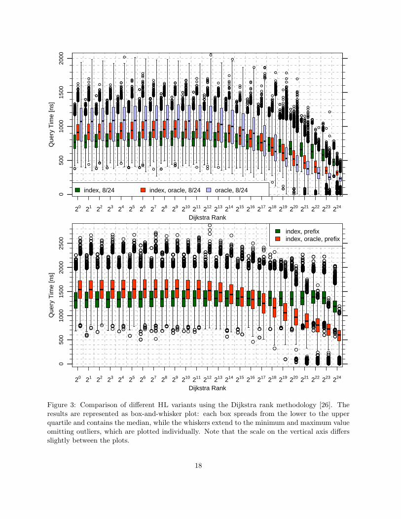
In the following, we report the (parallel) preprocessing time (without the CH preprocessing)and total space consumption in GB. Query performance is evaluated by running 100 000 000 s–tqueries, with s and t picked (in advance) uniformly at random. In most experiments, we reportaverage query times. Note that we use parallelization only during preprocessing; queries areexecuted on only one core. Also note that we consider the scenario in which only the shortestpath distance is to be computed, and not the full path. If full descriptions of the shortest pathsare needed, one could apply some of the path-expansion techniques used for TNR [3], for example.

The next section studies the impact of various design decisions on the performance of ouralgorithm. This will allow us to pick the best set of parameters for our algorithm in differentscenarios. In Section 6.2, we compare these optimized versions of HL with other methods in theliterature.

6.1 Trade-offs and Parameter Tuning

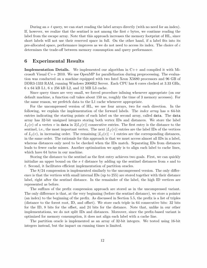
Impact of Label Pruning. Our first experiment studies how different label-pruning strategiesaffect label size and query performance. The input is the augmented graph produced by theCH algorithm; we build the labels by running upward searches on this graph. We tested thefollowing pruning strategies: 1-hop heuristic, 2-hop heuristic, and 1-hop heuristic combined withbootstrapping. The results can be found in Table 1. Note that we do not use any compression inthis experiment.

preprocessing querieslabel vertices space time

boot hops time [s] /label [GB] [ns]× 0 321 536.31 154.4 > 3000× 1 385 133.03 37.0 937× 2 491 113.05 31.5 834X 1 580 109.62 30.6 812

Table 1: Impact of label pruning on the performance of HL. We consider heuristic pruning withvariable number of hops and exact pruning (bootstrapping).

The first row in the table estimates the performance of our algorithm with no pruning, i.e.,if we used the entire CH search space as labels. Note that we did not actually run this variantin full, as it requires more memory than our machine has. The numbers provided are estimatesbased on sampling.

13

Among the pruned variants, observe that the 1-hop strategy already reduces the average labelsize by a factor of 4. Bootstrapping reduces the sizes of the labels even further, which also has apositive effect on query performance. Since bootstrapping does not slow down the preprocessingby too much, we use it by default, combined with the heuristic 1-hop pruning.

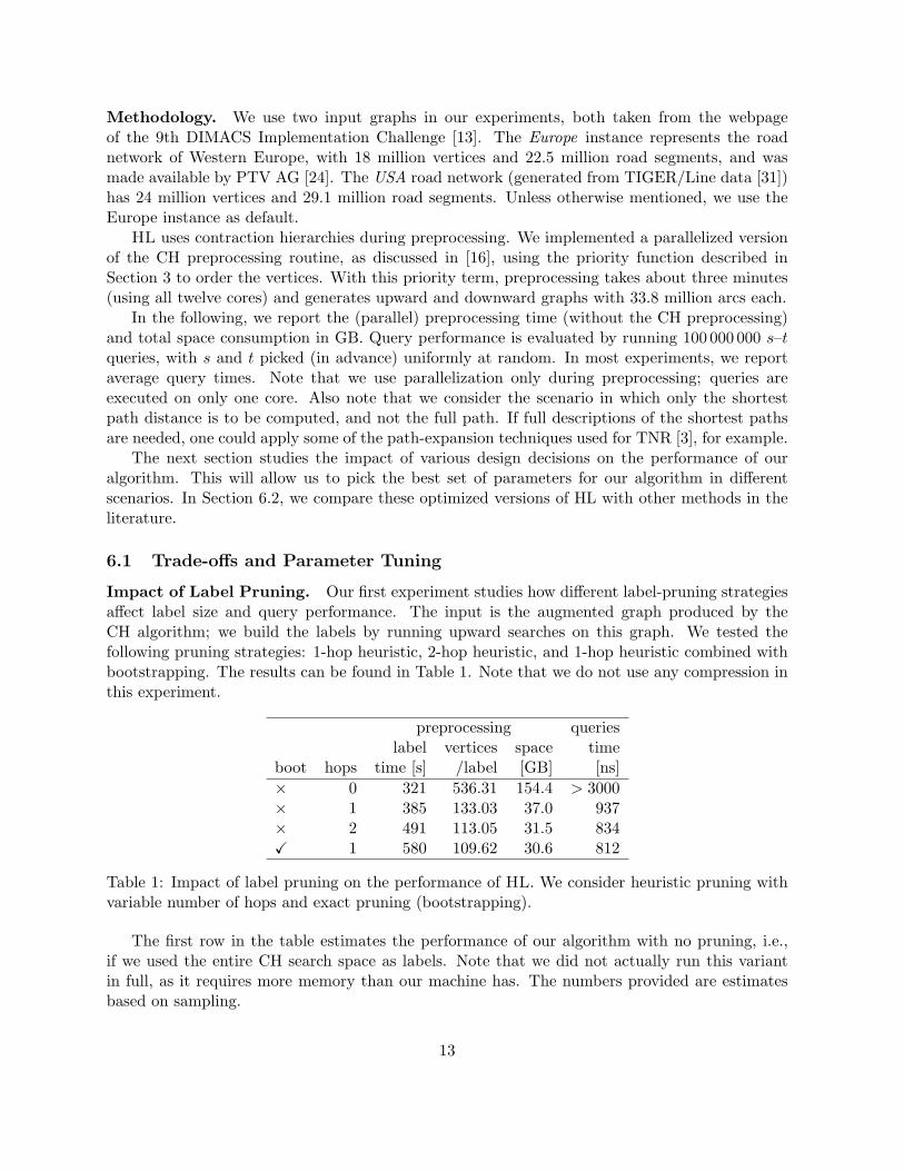
Impact of Label Ordering. As explained in Section 5, the order in which vertices are repre-sented within the labels may have an impact on query performance. In Table 2, we consider sixdifferent strategies to assign internal IDs to vertices. The first (input) just keeps the initial inputIDs. Second, we consider an inverted level assignment, in which higher-level vertices are assignedlower IDs, with the input order maintained within each level. The third and fourth strategies inthe table consisting of “promoting” only the 256 highest-ranked vertices (according to the CHpreprocessing), keeping the remaining vertices in input order. The two variants of this strategydiffer on whether the 256 most important vertices are sorted in input or level order. Finally, weconsider sorting all vertices in level and rank order.

preprocessing querieslabel vertices space time

ordering time [s] /label [GB] [ns]input 580 109.62 30.6 812inverted level 705 109.62 30.6 1134top 256 input 451 109.62 30.6 769top 256 level 469 109.62 30.6 812level 629 109.62 30.6 1155rank 651 109.62 30.6 1143inverse rank 599 109.62 30.6 1128

Table 2: Impact of label vertex ordering on the performance of HL.

Overall, keeping the original order for most vertices seems to be a good idea. Rearrangingthem by level (either ascending or descending) or rank has a negative impact on performance.This can be explained by the fact that there is locality in the original order: the IDs of nearbyvertices in the graph are likely to be similar. Moreover, if two small regions are far from eachother, it is often the case that all vertex IDs in one region are larger than all vertex IDs in theother. In particular, during an s–t query, this is often true for the regions around s and aroundt, which constitute a large portion of their respective labels. Recall that an HL query keeps onepointer for each label, advancing in each step the one pointing to the lowest ID. Because of thelocality in the input, it often reaches the end of one label (thus stopping the search) while visitinga fraction of the other. Rearranging vertices by level or rank destroys this locality and decreasesquery performance.

We can, however, obtain additional performance gains by making the 256 most importantvertices have the lowest IDs, while keeping the input order for the remaining vertices. For randomqueries, where s and t tend to be far apart, most searches meet only at these vertices. By keepingthem close in the label, we improve locality when accessing actual distances. Unless otherwisestated, we use a top 256 input ordering as default for the remainder of this paper.

14

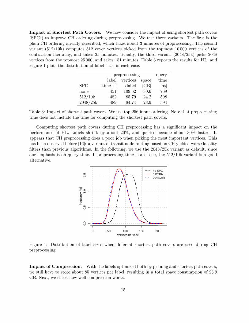
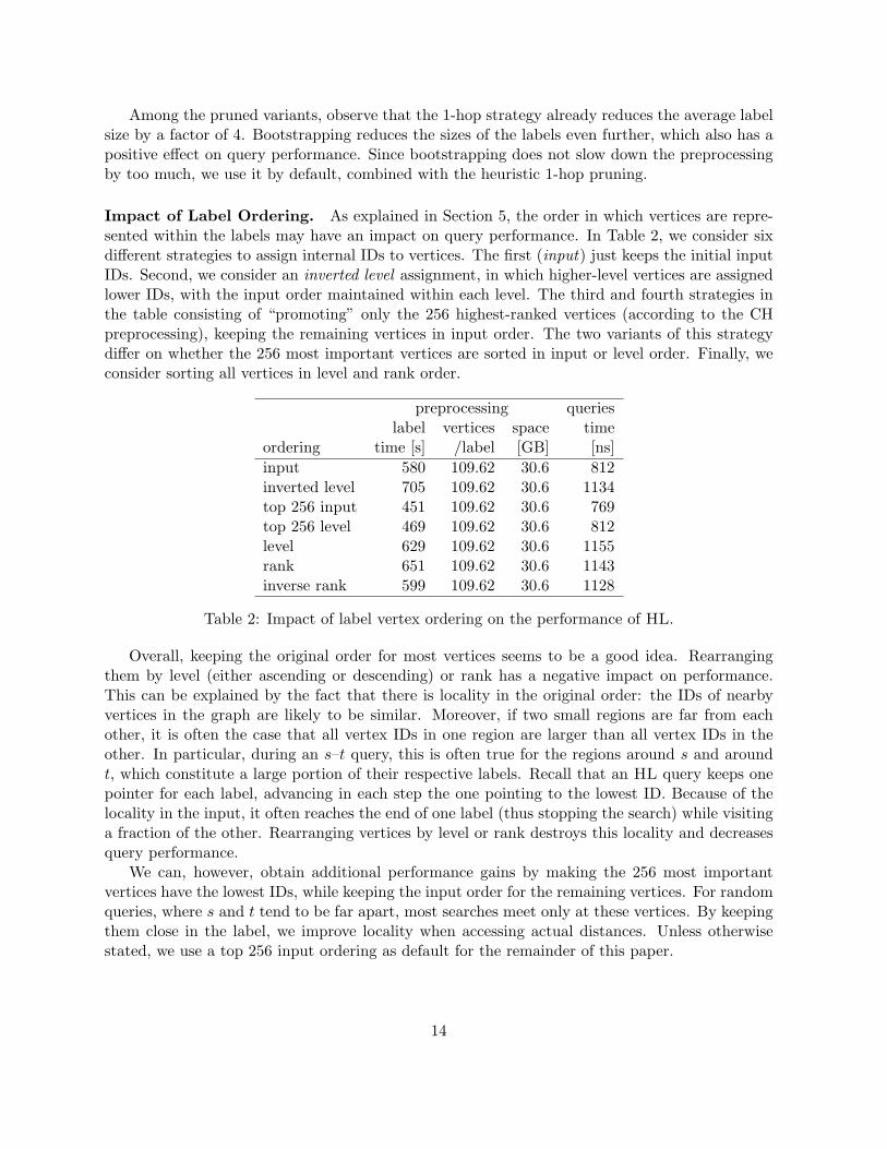
Impact of Shortest Path Covers. We now consider the impact of using shortest path covers(SPCs) to improve CH ordering during preprocessing. We test three variants. The first is theplain CH ordering already described, which takes about 3 minutes of preprocessing. The secondvariant (512/10k) computes 512 cover vertices picked from the topmost 10 000 vertices of thecontraction hierarchy, and takes 25 minutes. Finally, the third variant (2048/25k) picks 2048vertices from the topmost 25 000, and takes 151 minutes. Table 3 reports the results for HL, andFigure 1 plots the distribution of label sizes in each case.

preprocessing querylabel vertices space time

SPC time [s] /label [GB] [ns]none 451 109.62 30.6 769512/10k 482 85.79 24.2 5982048/25k 489 84.74 23.9 594

Table 3: Impact of shortest path covers. We use top 256 input ordering. Note that preprocessingtime does not include the time for computing the shortest path covers.

Computing shortest path covers during CH preprocessing has a significant impact on theperformance of HL. Labels shrink by about 20%, and queries become about 30% faster. Itappears that CH preprocessing does a poor job when picking the most important vertices. Thishas been observed before [16]: a variant of transit node routing based on CH yielded worse localityfilters than previous algorithms. In the following, we use the 2048/25k variant as default, sinceour emphasis is on query time. If preprocessing time is an issue, the 512/10k variant is a goodalternative.

vertices per label

freq

uenc

y [%

]0.

00.

51.

01.

5

0 50 100 150 200

no SPC512/10k2048/25k

Figure 1: Distribution of label sizes when different shortest path covers are used during CHpreprocessing.

Impact of Compression. With the labels optimized both by pruning and shortest path covers,we still have to store about 85 vertices per label, resulting in a total space consumption of 23.9GB. Next, we check how well compression works.

15

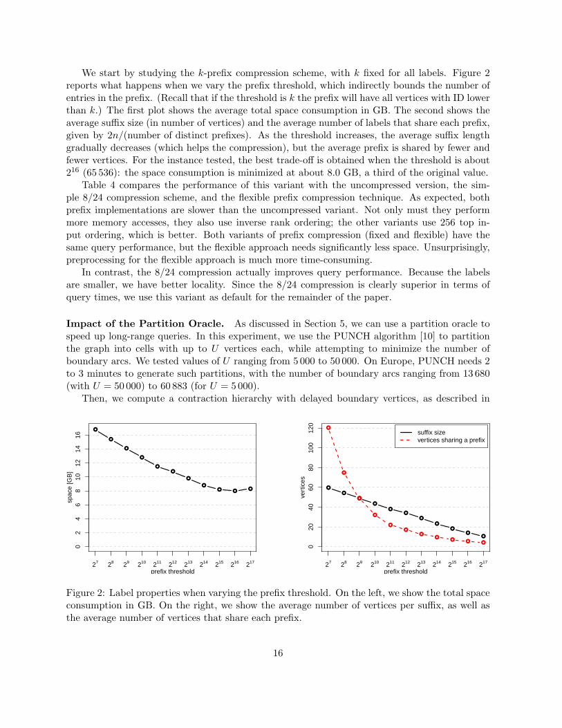
We start by studying the k-prefix compression scheme, with k fixed for all labels. Figure 2reports what happens when we vary the prefix threshold, which indirectly bounds the number ofentries in the prefix. (Recall that if the threshold is k the prefix will have all vertices with ID lowerthan k.) The first plot shows the average total space consumption in GB. The second shows theaverage suffix size (in number of vertices) and the average number of labels that share each prefix,given by 2n/(number of distinct prefixes). As the threshold increases, the average suffix lengthgradually decreases (which helps the compression), but the average prefix is shared by fewer andfewer vertices. For the instance tested, the best trade-off is obtained when the threshold is about216 (65 536): the space consumption is minimized at about 8.0 GB, a third of the original value.

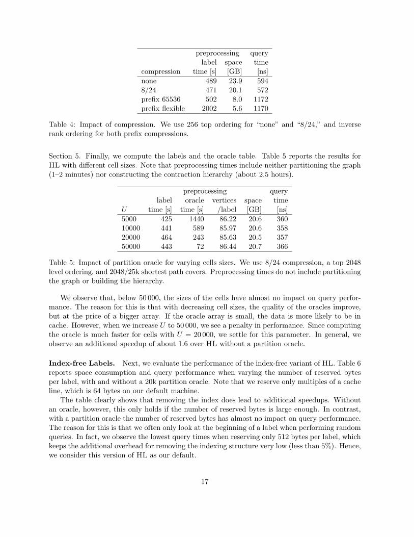
Table 4 compares the performance of this variant with the uncompressed version, the sim-ple 8/24 compression scheme, and the flexible prefix compression technique. As expected, bothprefix implementations are slower than the uncompressed variant. Not only must they performmore memory accesses, they also use inverse rank ordering; the other variants use 256 top in-put ordering, which is better. Both variants of prefix compression (fixed and flexible) have thesame query performance, but the flexible approach needs significantly less space. Unsurprisingly,preprocessing for the flexible approach is much more time-consuming.

In contrast, the 8/24 compression actually improves query performance. Because the labelsare smaller, we have better locality. Since the 8/24 compression is clearly superior in terms ofquery times, we use this variant as default for the remainder of the paper.

Impact of the Partition Oracle. As discussed in Section 5, we can use a partition oracle tospeed up long-range queries. In this experiment, we use the PUNCH algorithm [10] to partitionthe graph into cells with up to U vertices each, while attempting to minimize the number ofboundary arcs. We tested values of U ranging from 5 000 to 50 000. On Europe, PUNCH needs 2to 3 minutes to generate such partitions, with the number of boundary arcs ranging from 13 680(with U = 50 000) to 60 883 (for U = 5000).

Then, we compute a contraction hierarchy with delayed boundary vertices, as described in

prefix threshold

spac

e [G

B]

27 28 29 210 211 212 213 214 215 216 217

02

46

810

1214

16

●

●

●

●

●

●

●

●● ●

●

prefix threshold

vert

ices

27 28 29 210 211 212 213 214 215 216 217

020

4060

8010

012

0

●

●

●

●

●●

●

●

●●

●

●

●

●

●

●●

●●

● ● ●

suffix sizevertices sharing a prefix

Figure 2: Label properties when varying the prefix threshold. On the left, we show the total spaceconsumption in GB. On the right, we show the average number of vertices per suffix, as well asthe average number of vertices that share each prefix.

16

preprocessing querylabel space time

compression time [s] [GB] [ns]none 489 23.9 5948/24 471 20.1 572prefix 65536 502 8.0 1172prefix flexible 2002 5.6 1170

Table 4: Impact of compression. We use 256 top ordering for “none” and “8/24,” and inverserank ordering for both prefix compressions.

Section 5. Finally, we compute the labels and the oracle table. Table 5 reports the results forHL with different cell sizes. Note that preprocessing times include neither partitioning the graph(1–2 minutes) nor constructing the contraction hierarchy (about 2.5 hours).

preprocessing querylabel oracle vertices space time

U time [s] time [s] /label [GB] [ns]5000 425 1440 86.22 20.6 36010000 441 589 85.97 20.6 35820000 464 243 85.63 20.5 35750000 443 72 86.44 20.7 366

Table 5: Impact of partition oracle for varying cells sizes. We use 8/24 compression, a top 2048level ordering, and 2048/25k shortest path covers. Preprocessing times do not include partitioningthe graph or building the hierarchy.

We observe that, below 50 000, the sizes of the cells have almost no impact on query perfor-mance. The reason for this is that with decreasing cell sizes, the quality of the oracles improve,but at the price of a bigger array. If the oracle array is small, the data is more likely to be incache. However, when we increase U to 50 000, we see a penalty in performance. Since computingthe oracle is much faster for cells with U = 20 000, we settle for this parameter. In general, weobserve an additional speedup of about 1.6 over HL without a partition oracle.

Index-free Labels. Next, we evaluate the performance of the index-free variant of HL. Table 6reports space consumption and query performance when varying the number of reserved bytesper label, with and without a 20k partition oracle. Note that we reserve only multiples of a cacheline, which is 64 bytes on our default machine.

The table clearly shows that removing the index does lead to additional speedups. Withoutan oracle, however, this only holds if the number of reserved bytes is large enough. In contrast,with a partition oracle the number of reserved bytes has almost no impact on query performance.The reason for this is that we often only look at the beginning of a label when performing randomqueries. In fact, we observe the lowest query times when reserving only 512 bytes per label, whichkeeps the additional overhead for removing the indexing structure very low (less than 5%). Hence,we consider this version of HL as our default.

17

●

●●●●●●●●●

●●●●

●

●●

●●●

●●●●●●●

●

●●●●

●

●●

●●

●

●

●●●●●●●●

●

●●

●

●

●

●

●

●●

●

●●●

●●

●

●●

●

●●

●

●●

●

●●

●

●●

●●●●

●●

●●

●●●

●

●

●●●●●●

●

●●●●●

●●●

●●●●●●●●●●

●

●

●

●

●

●

●●

●

●●

●●●●●●

●

●●●●●●

●●●●●●●●●●●●●●

●

●●●

●

●●

●

●●

●●●●●

●

●

●●●

●●●

●●●●

●

●●●●●●●●●●

●●●●●

●●

●●●●●

●●●●●●●

●●

●

●●●

●

●●●●●●

●

●

●●●

●

●

●●

●●

●●●

●●

●●●●●

●

●●

●

●●●

●

●

●

●

●●

●●

●

●

●

●

●●●●●

●●

●●●●●●●●●●●●●

●

●

●

●

●

●

●

●●

●●

●●

●

●●●

●●

●●

●●●●●

●

●●●●●●

●●●

●

●●

●

●●●●●

●

●●●

●●

●

●

●

●●

●●●

●

●●●

●

●

●●

●●●

●

●

●

●●

●●●●

●

●

●●

●

●

●●●●●●●●

●

●

●

●

●●●●●●

●

●

●●●●●●●●●●

●

●●●●

●

●●

●

●●●●

●

●●

●

●

●

●●

●

●●●

●

●●

●

●

●●

●

●●●●

●

●

●

●

●●●

●

●●●●●●

●●●

●

●

●●

●

●

●●

●●

●

●

●

●

●●

●

●●

●

●●●●●●●●●●●● ●

●

●●

●

●

●●●●

●●●

●

●●●

●

●

●

●●

●

●

●

●●●●●●●●●●●

●

●●●●

●

●

●●●●●●

●

●

●●●

●●

●

●

●●●

●●●●●●●

●

●●●●●

●

●●●●●●

●

●●●●●●●●●●●●●●

●●●●

●●●

●

●

●●●●●

●●●

●

●

●●●●●

●●●

●●

●

●●●●●●●

●●●●●●

●●●●

●

●●

●

●

●●●●●●●●●●●●

●

●●●●

●

●●

●

●●

●●

●

●●

●

●●●

●

●

●●

●

●●

●●

●●●

●●

●

●

●●●●●●●●

●●

●●

●●●●●

●

●●●

●

●

●

●●

●●

●

●

●●●

●

●●●●●●

●

●●●●●●●●

●

●●●

●●

●●●●●●●●

●●●●●●●

●●●●

●

●●

●

●●●●●●●●●●●●●●●●●●

●

●●

●●●●●●●

●●●

●

●

●

●●

●

●

●

●●●●●

●

●

●

●●

●●●●●●●●●

●

●

●

●●●●

●

●●●●●●●●

●●

●

●

●●

●●●

●●

●●●

●

●●●●

●

●●●

●

●

●●

●

●

●

●

●●●●

●●●●●●●●●●●

●

●

●

●●●●

●●

●

●●

●●●●●●●

●

●

●

●●

●●●●●●

●

●●●●●

●●●●●

●

●●●

●●

●

●

●

●

●●●●●●

●

●●●●

●

●●●●

●

●●●●

●●●●●●

●●

●

●

●●●●●●●

●

●●●

●

●●

●●●

●

●

●

●●●

●●●

●●

●

●

●●●

●

●

●●

●

●●●●●●●

●●

●

●

●

●

●●

●

●●●

●●

●

●●●●●●●●

●

●

●●

●

●●

●

●●●●●●●●

●

●●

●

●●●

●●

●●●●●●●●●●●

●

●

●●●●●●

●

●●

●

●●●

●

●●●●●

●●

●

●●●●●●●

●

●

●

●●●●●

●●●

●

●●●

●●●●

●●●

●

●

●

●●●●●●●

●●●●●●

●●●

●

●●

●●

●

●●●●●●●●●●●●●●●●●●●

●

●●●●●●●

●●

●

●●●●●●●●●

●

●

●

●

●●●●●●●●●●●●●●●●●●●●●●●●●●●●●● ●●●

●●●

●

●●●●

●●

●●●●●●●●

●

●●●●●●● ●●

●

●●●●●●●

●●●●●●●●●●●●●

●

●

●●

●

●

●●●●●●●●●●●

●

●●●

●

●

●

●●

●●●

●

●●

●

●●●●●●●●●

●

●●●

●

●

20 21 22 23 24 25 26 27 28 29 210 211 212 213 214 215 216 217 218 219 220 221 222 223 224

050

010

0015

0020

00

index, 8/24 index, oracle, 8/24 oracle, 8/24

●

●●●●●●●●●

●●●●

●

●●

●●●

●●●●●●●

●

●●●●

●

●●

●●

●

●

●●●●●●●●

●

●●

●

●

●

●

●

●●

●

●●●

●●

●

●●

●

●●

●

●●

●

●●

●

●●

●●●●

●●

●●

●●●

●

●

●●●●●●

●

●●●●●

●●●

●●●●●●●●●●

●

●

●

●

●

●

●●

●

●●

●●●●●●

●

●●●●●●

●●●●●●●●●●●●●●

●

●●●

●

●●

●

●●

●●●●●

●

●

●●●

●●●

●●●●

●

●●●●●●●●●●

●●●●●

●●

●●●●●

●●●●●●●

●●

●

●●●

●

●●●●●●

●

●

●●●

●

●

●●

●●

●●●

●●

●●●●●

●

●●

●

●●●

●

●

●

●

●●

●●

●

●

●

●

●●●●●

●●

●●●●●●●●●●●●●

●

●

●

●

●

●

●

●●

●●

●●

●

●●●

●●

●●

●●●●●

●

●●●●●●

●●●

●

●●

●

●●●●●

●

●●●

●●

●

●

●

●●

●●●

●

●●●

●

●

●●

●●●

●

●

●

●●

●●●●

●

●

●●

●

●

●●●●●●●●

●

●

●

●

●●●●●●

●

●

●●●●●●●●●●

●

●●●●

●

●●

●

●●●●

●

●●

●

●

●

●●

●

●●●

●

●●

●

●

●●

●

●●●●

●

●

●

●

●●●

●

●●●●●●

●●●

●

●

●●

●

●

●●

●●

●

●

●

●

●●

●

●●

●

●●●●●●●●●●●● ●

●

●●

●

●

●●●●

●●●

●

●●●

●

●

●

●●

●

●

●

●●●●●●●●●●●

●

●●●●

●

●

●●●●●●

●

●

●●●

●●

●

●

●●●

●●●●●●●

●

●●●●●

●

●●●●●●

●

●●●●●●●●●●●●●●

●●●●

●●●

●

●

●●●●●

●●●

●

●

●●●●●

●●●

●●

●

●●●●●●●

●●●●●●

●●●●

●

●●

●

●

●●●●●●●●●●●●

●

●●●●

●

●●

●

●●

●●

●

●●

●

●●●

●

●

●●

●

●●

●●

●●●

●●

●

●

●●●●●●●●

●●

●●

●●●●●

●

●●●

●

●

●

●●

●●

●

●

●●●

●

●●●●●●

●

●●●●●●●●

●

●●●

●●

●●●●●●●●

●●●●●●●

●●●●

●

●●

●

●●●●●●●●●●●●●●●●●●

●

●●

●●●●●●●

●●●

●

●

●

●●

●

●

●

●●●●●

●

●

●

●●

●●●●●●●●●

●

●

●

●●●●

●

●●●●●●●●

●●

●

●

●●

●●●

●●

●●●

●

●●●●

●

●●●

●

●

●●

●

●

●

●

●●●●

●●●●●●●●●●●

●

●

●

●●●●

●●

●

●●

●●●●●●●

●

●

●

●●

●●●●●●

●

●●●●●

●●●●●

●

●●●

●●

●

●

●

●

●●●●●●

●

●●●●

●

●●●●

●

●●●●

●●●●●●

●●

●

●

●●●●●●●

●

●●●

●

●●

●●●

●

●

●

●●●

●●●

●●

●

●

●●●

●

●

●●

●

●●●●●●●

●●

●

●

●

●

●●

●

●●●

●●

●

●●●●●●●●

●

●

●●

●

●●

●

●●●●●●●●

●

●●

●

●●●

●●

●●●●●●●●●●●

●

●

●●●●●●

●

●●

●

●●●

●

●●●●●

●●

●

●●●●●●●

●

●

●

●●●●●

●●●

●

●●●

●●●●

●●●

●

●

●

●●●●●●●

●●●●●●

●●●

●

●●

●●

●

●●●●●●●●●●●●●●●●●●●

●

●●●●●●●

●●

●

●●●●●●●●●

●

●

●

●

●●●●●●●●●●●●●●●●●●●●●●●●●●●●●● ●●●

●●●

●

●●●●

●●

●●●●●●●●

●

●●●●●●● ●●

●

●●●●●●●

●●●●●●●●●●●●●

●

●

●●

●

●

●●●●●●●●●●●

●

●●●

●

●

●

●●

●●●

●

●●

●

●●●●●●●●●

●

●●●

●

●

●●●

●

●●

●

●

●●●●

●

●●●

●●●

●

●●

●●

●

●

●

●

●

●●

●●

●

●●●●●●

●●

●●

●

●●

●●

●

●

●●●●

●

●

●●

●

●

● ●●

●●

●●●

●

●

●

●

●

●●●●

●●

●

●

●

●

●●●

●●●

●●

●

●●●

●

●

●●●●●●●●●●●

●●

●

●

●

●

●●

●●●

●●●●

●

●●

●

●●●

●●●●

●

●●

●●

●

●●

●

●●●

●

●●

●●●

●

●

●●●●

●

●

●●●

●●●●●●●●

●●●●

●

●●●●●●

●

●●

●●●●●●

●

●

●●●●

●●●●●●●

●●

●●

●●

●

●

●●

●●

●

●●

●●

●

●●

●

●●

●

●

●

●

●●●●

●

●

●

●

●●

●

●

●●●●●

●●

●

●●●●●●●●●

●

●

●

● ●●●

●

●●●●

●

●

●

●●●●●●●●●●

●●●●●●

●

●●●●●

●●●●●

●●

●●●

●

●

●●●

●●●●

●●●●

●

●●

●

●●

●

●●●

●

●

●

●

●

●●●●

●

●

●●●●●

●

●●

●

●●

●

●

●●

●●

●

●●

●●

●

●

●

●●●●●

●

●

●●● ●

●

●●●

●

●

●

●

●

●

●●●●

●

●

●

●

●

●●●●●

●

●●●

●

●

●●

●

●

●

●●●●

●

●●

●

●●

●

●

●

●

●

●●

●

●

●

●

●●

●

●●

●

●

●●●●

●

●●●

●

●●

●●

●

●●●●●

●

●

●

●●●●

●

●

●

●

●

●●●●

●

●●

●●●●

●

●●●●

●

●

●

●●

●

●

●●●●●

●

●

●●●

●

●

●●●

●●

●

●●●●●●●●●●

●●●●

●

●

●

●

●●

●

●●

●●●

●●

●

●

●

●

●

●● ●●●

●

●

●●●●

●●

●●●●

●

●●●●●

●

●

●●●

●

●

●

●●●●●

●●

●

●

●

●●

●

●●

●

●

●

●

●

●●●

●

● ●●●

●●

●●

●

●

●●●●

●

●●●

●●●

●

●

●●●

●●

●

●

●

●●●●

●●●●●●●

●

●

●●●●

●

●●●●●●

●●●

●

●

●●●●●

●●

●

●

●●●●●

●

●●●

●●●

●●●●●

●

●

●

●●

●

●●

●

●

●●●

●

●

●●●

●

●●●

●

●

●●●●●●

●

●●●●●

●

●

●

●

●

●●

●

●●

●● ●

●

●●●

●●●

●

●

●

●●●●●

●●

●●

●

●●

●●

●●●●

●●●●●●●●

●

●

●

●●●●●

●

●

●● ●●

●

●

●

●

●

●●

●●●●●●

●

●

●●●●●●

●

●

●●

●●●

●

●●●●●

●●

●

●

●

●●●●

●

●

●

●●

●●●●●●●●●●●

●●●

●

●●●

●

●●●●

●

●●●●

●

●

●●●●

●

●

●

●●

●●●●●●●●

●

●

●

●

●

●●●●

●●●●

●

●●●●●●●●

●

●

●

●

●●●●●

●

●

●

●●

●

●●

●

●

●

●

●

●●●

●

●●●

●

●●●●●●●

●●

●

●●●●●●●●

●

●●

●

●●●

●

●

●

●●

●●

●

●●

●●●

●

●●

●●●●●●

●

●●

●

●

●●●

●

●●●●

●

●●

●●●●●●

●●

●●

●

●●

●●● ●

●●

●

●

●

●●

●●

●●

●

●

●

●

●●●

●

●●

●

●

●●●

●●●

●●

●

●

●●●

●

●

●

●●

●

●

●

●●●●●

●●●

●

●

●

●

●

●

●●●●

●

●●●●

●

●●●●●

●

●

●

●

●●

●

●

●●

●

●●●

●

●

●

●

●

●

●

●

●

●●●●●

●●●●

●

●

●●●

●●

●●●

●

●

●

●●

●

●●●

●

●●

●

●●

●●

●

●

●

●●

●

●

●

●

●●●●

●

●

●

●

●●

●

●

●

●

●●

●

●

●●

●

●

●

●●●●

●

●

●●

●●●

●

●

●

●●●

●●

●

●

●●●●

●

●

●

●

●●

●

●

●●●●●●●

●

●●●●●

●●●●

●

●

●

●●●●

●

●

●

●●●

●

●●●●

●

●●●●●

●

●●●●●●

●

●●●●●

●●●●●●

●

●●●●

●

●●●

●

●●●●●●●●

●

●●●●●●

●

●●

●

●●●

●

●●●

●

●●

●

●●

●●●●●

●

●●●●●

●●●●●

●

●●●●●●●●●●

●

●

●

●●●●

●

●●●●

●●

●●

●●●●●●●●●●

●

●

●●●●●

●

●

●●

●

●

●●

●

●●●

●

●

●●●●

●

●●●

●●●

●●

●●●

●

●

●●●●●●●●●

●

●

●●●●●●

●

●●●

●

●

●

●●●●●

●

●●●●●

●

●●●●

●

●●●

●

●

●

●

●

●●

●

●●●●●

●●●

●

●●

●

●

●

●

●

●●●●●●

●●●●●●●●

●

●●●

●

●●

●

●●

●●●●●●●●

●

●●●

●●

●●●●●●●●●●●

●●

●

●●●

●●●●●

●

●●●●

●

●●●●●●●

●

●

●

●

●

●●

●

●

●●●●

●●

●●

●

●●●●

●

●●●●●

●

●●●●●●●

●

●●●●●

●

●

●●

●

●

●●

●●●

●

●●●

●

●●●

●●●●●●●

●●●●●

●

●

●

●

●●

●

●

●●●●●●

●

●●●

●

●

●●●●●●●●●●●●●●

●

●

●

●●●●●●●●

●

●●●●●●●●●

●

●●●●●●●●●●●●●●●

●●●

●

●●●●●●●●●●

●

●●●●●●●

●

●

●

●

●●●●●●

●

●●●●●●●●●●●

●

●●

●●●

●●●●●●●

●

●

●

●●●●●●●●

●

●

●●

●●

●

●●●●●●●

●

●

●

●●●●

●

●●●●●●●●●●

●

●●●●●●●●●●●●●●●

●●●●●●●●

●●●

●●

●●●●

●

●

●

●

●

●●

●

●

●●●

●

●

●

●●●●●

●

●

●●●●●

●

●

●

●

●

●

●

●●●

●

●

●●

●

●

●

●

●●●

●●●

●

●

●

●●

●

●

●

●

●

●●●

●

●

●

●

●●

●

●

●

●

●

●●

●

●●●●

●

●●●●

●

●

●

●

●

●●

●●●●●●

●

●

●●

●●●●

●●

●●

●

●

●●●

●●●

●

●

●●

●

●

●

●●●

●

●

●●

●●

●

●

●●●●●●●●

●

●●

●●

●●

●

●●

●●

●

●

●●

●

●●●

●●●

●●●●

●

●●●●

●

●●●

●

●●

●●

●

●●●●●●●

●

●●

●

●●●

●

●●●●●●●●●●●●●

●

●●●●●●●●●●●●●●●●●●●●●●

●

●●●●●●●●●●●●●●●●●●●●●●●●●●●●●●●●●●

●

●

●

●●●●

●

●

●●●

●

●●●●●●●●●

●●

●

●●

●

●●●

●

●

●

●●●

●

●●

●●●●

●

●●●●●●●●

●

●●●●●●●●●

●

●●●●●●●●●

●

●●●●●●●●●●●●●●●●●

●●●●●●

●

●●

●

●●●●●●●

●●●●

●

●●●●●●●●●●●●●●●●●●

●

●●●●●●●●●

●

●●●●●●●●●●

●

●●

●

●●●●●●●●●●●●●●●●●●

●

●

●

●●●

●●

●●

●

●●●●●●●●●●●●

●

●

●●●●●●●●●●●●●●●●●●

●●●●●●

●

●●●

●

●●●●●●●●●●

●

●●

●

●●●

●

●●●●●●

●

●●

●

●●●●●●●●●●●●

●●●●●●●

●●●●●

●

●●●●●●●●●●●

●

●●●●●●●●●●●

●

●

●

●●●●

●●●●●●

●

●●●●●●●●●●●●●●●●●●●●●●●●●●●●●●●●●●●●●

●

●●●●●●●●●●

●●●●●●●●●●●

●

●●●●●●●●●●●●●●●●

●

●●●●●●

●

●

●

●●

●

●

●

●●●

●

●

●

●

●

●●●●

●●

●●●

●

●●

●

●●

●

●

●●

●

●●●●

●

●●●●●●●●

●

●●●

●

●●●●●●●●●●●●●●●●●●●●●●●●●●

●

●●

●

●●

●

●●●●●●●●●●●●●●●●●●

●●●

●

●

●

●●

●

●●●●●●●●●●●●●●●●●●●●●●●●●●●●●●●●●●●

●

●●●●

●●●●●●●●

●

●

●

●●●●

●

●●●●●●●●●●

●

●●●

●

●●●

●

●●●●●●●●●●

●

●●

●

●●●●●●●●●●●●●●

●

●●●●●●

●

●●●●

●

●●

●

●●

●

●●●●●●●●●●●●

●

●

●

●●

●

●●●●●●●●●●●●●●●

●

●●●●●

●●●●●●●●●●

●

●●●●●

●

●●●

●

●●●●●●●●●

●

●●

●

●

●

●●●●●●●●●●●

●

●●●●●●●

●

●●●●●●●

●

●●●●●●●●

●

●●●●

●●●●●●

●

●●●●●●●

●

●

●

●●●●●●●●●●

●

●●●●●●●

●

●●●●

●

●●

●

●●●●●●●●●●●●●●●

●

●●

●

●●●●●●

●

●

●

●

●

●

●●●●

●

●●●●●●●●●●●●●●●●●●●●●●●●●●●●●●

●

●●

●

●●●●●●●●

●

●●●●

●

●

●

●●●●●●●●●●

●

●●●●●●●●

●

●

●

●

●

●●●●●●●

●●●●●●●●●

●

●

●

●●●

●

●●●●●●●

●

●●●●●●●●●●●●●●●●●●

●

●●●●●●●●●●

●

●●●●●

●

●●●

●

●●

●

●

●●●●●●●

●

●●●●●●●●●●●●●●

●

●●●●●●

●

●

●●●

●

●●●●●●●●●●●●●●●●●●

●

●●

●

●

●

●

●●

●

●●●●●●●●●●●●●●●●●●●●●●●

●

●●●●●●

●●●●●●●●

●

●

●●●●●

●

●●●●●●●●●●

●

●●●

●●●●●

●

●●●●●●●●●●●●●●●●●●●

●●●●

●

●

●●●●●●●●●●●●●

●

●●●

●

●

●●●●●●●●●●●

●

●●●●●●●●●

●

●●●●●●●●●●

●

●●●●●●●

●

●●●●●●●●

●●

●

●

●

●

●●●●●●●●

●

●●●●●●●●●●●●●●●●●●●●●●●●●●

●

●

●

●

●

●●●●

●●●●●●

●

●

●●●●●

●●●●

●

●●●●●●●●

●

●●

●

●●●

●●●●●●●●●●●●●●●●

●

●●●●●

●

●●●

●

●

●

●

●●●●●●●●●●●●●

●

●●●●●

●

●

●

●●●●●●●●●●●●●●●●

●

●

●

●●

●

●

●●●●

●●

●●●●●●●●●●

●

●

●

●●●●●

●

●●●●

●

●●●●●●●●●●●●●●●●●●●●

●

●●●●●●●●●●

●

●

●●●●●●●●●●●●●●●●●●●●●●●●●●●●●●●●●

●

●●●●●●●

●

●●●●●●●

●

●●●●●●●●

●

●

●●●●●●●●●●

●

●●

●●●●●●●●●

●

●●●●●●●●●

●

●●●●

●

●●●●●

●

●●●●●●●

●

●●●

●

●●

●●●●●●

●●

●●●

●

●●●●●●●●●●●●

●●

●

●●●

●

●●●

●

●●●

●

●●●●●●●●●●●●●●●●●●●●●●●

●

●●

●●●●●●●●●●●●●●

●

●●●●●●●●●●●●

●

●●●●●●●●●●●●●●●●●

●

●●

●●

●

●

●

●

●

●

●●

●●●●●

●●●●●●●●●●●●

●

●●●●●●●

●●

●●●

●

●●●●

●

●●

●

●●●

●

●●

●●●●●●●

●●●●●●●●●●●●●

●

●

●●●●●●●●●

●

●

●●●●●●●●●●

●

●●●

●

●

●

●

●

●●●

●●●●●●●●●●●●●●

●

●●●●●

●

●●●

●

●●●●●●●●●●●●●●

●

●●●●●●

●

●●●●●●●●●

●●

●●●●●●●●●

●

●●●

●

●

●

●●●●●

●

●●

●

●●●●●●●●●●

●

●●

●

●●

●

●●●●●●●●●

●

●

●

●●●●

●●●●●●●

●

●●

●●●●●●●●●

●●●

●●●●●●●●●●●●

●

●

●●●●●

●●

●

●

●

●●

●

●

●●●●●●●

●

●

●

●●●●●●●●●

●●●

●

●

●

●●●

●

●●●●●●●

●

●

●●●●●●

●

●

●

●●●●●●●●●●●●●●●●●●

●

●●●●●●●●●●●

●

●●●●●●●●●●●●●●●●●●

●

●

●●●

●●●●●

●

●

●●●●●●●●●

●

●●

●

●

●

●

●

●●

●●

●●●●●

●●●

●

●●●●●●●●●●●●●

●

●●●

●●●●●●●●●●

●

●●

●●●●●●●●●●●

●

●●●●●

●

●

●●●●

●

●●●●●●●

●

●●●●●●●●●●●●●●●●●●

●

●●●●●

●

●●●●

●

●●●●

●

●

●

●●●●●●

●

●●●●

●

●●●●●●●●●●●●●●●●

●●●●●●●●●●●

●●●●●●●

●●●●●●●●●●●●●●●●●●

●

●●●●●●●●●●

●●●●●●●

●

●●●●●●●●●●●

●

●●

●

●

●

●

●

●●●●●●●●●

●●●●●

●

●●●

●●●●●●●●●●●●●●●●●●

●

●●●●●●●

●

●●●●●●●●

●●

●

●

●

●●●

●●

●●

●

●●●●●●●●●

●

●

●●●●●●

●

●●●●●●●●●●●●●●

●

●●●●

●

●

●

●●●●●●

●

●

●●●●●●●●●●

●

●●●●●●●●●●●●●●●

●

●●

●

●

●

●●

●

●●●●●●●●●●●●●●●

●●●●●

●

●●●●●●●

●

●

●

●●

●●

●●●●●

●

●●●●●

●

●●●●●

●●●●●●●●

●●●●●●●●●●

●

●●●●●●

●●

●

●●●

●

●●●●●

●●●●

●

●●●●●●●

●

●●●●●●●●●●●

●

●●●

●

●●●●●●●

●

●

●●●●●

●●

●

●

●●●●●

●●

●

●●●●

●●●●●●●●●

●

●●●●●

●●●

●

●●●

●

●●●●

●●●●●

●

●●●

●

●●●●●●●●

●●●●●●●●●

●

●

●●●

●

●

●

●

●●●●

●

●●●●

●

●●

●

●●●

●

●

●●●●●●●

●

●●●●●●●

●

●

●

●●●●●

●

●

●

●●●

●

●●

●●

●

●●●●●●●●●●●●●●

●

●●

●

●

●

●●

●●●

●

●●●

●

●●

●

●●●●

●●●

●

●●●●●●●

●

●●●●●●●

●

●

●●●●

●●

●

●

●●

●

●

●●●

●

●●

●

●●●●●●●●●●●●●

●

●

●●●●●●●●●

●

●

●

●●

●

●●●●●●●

●

●●●●

●

●●●●●●●

●

●●●●●

●

●●●●

●●●●

●

●●

●

●●●●●

●●

●

●

●

●●

●

●●●●●●●●●●●●

●

●

●●●●●●●●

●

●●●●●●●●●●●

●●●

●

●●●●●

●●●

●●●●

●

●

●●

●

●●●●●●

●

●

●●●●●●●

●

●●

●●●●

●

●

●●

●

●●●●

●

●

●

●

●

●●●●

●

●●●●●

●●●●●●●●●●●●●●●●●

●

●

●

●●●●●●

●

●●●●●●●●●●●●●●●

●

●●●●●●●●

●●

●●●●●●●●

●

●

●●●●●●

●

●●●●●●

●●●●

●

●●●●●

●

●●●●●

●

●

●●

●●●●

●

●●●●●●●●●●●●

●

●●●●●●

●

●●●

●

●●●

●

●●●●

●

●●●●●●

●

●

●

●●●

●

●●●●●●●●●●

●

●

●

●

●

●●●●●●●●●●●●●●●●●●●●●

●

●

●●

●●●●●●●●●●●●●●●●●●●●●●●

●

●●●●●●●

●

●●●●

●●

●

●

●●

●●

●

●●

●

●●●

●●●●●

●●

●●●●●

●

●

●

●●●●

●

●●

●

●●●●●●●●●●●●●●●

●●●●●●●●●●●

●

●

●●●●●●●

●

●●●●●●●●●●●●●●●●●●

●

●●●●

●

●●

●

●●●●●●●●●●●●●

●

●●●●●●●

●

●●●●

●

●

●

●●●●●

●●●●●●●●●●●●●●

●

●

●●●●●●●

●●●●●●●●●●●●●●●●●

●

●

●●●●●●

●

●●●●●●●●●

●

●

●●●●●●●●●●●●●●●●●●●●●●●●●●●●●

●●●●●●●●●●●●●●●●●●●●●●

●

●●●●

●

●●●●●●●

●

●●●●

●●●●●●●●●●●●●●●

●●●●●●●●●●

●

●●●●●●●●●●●●●●

●

●●●

●

●●●●●

●

●

●

●●●●●●

●

●●●

●●

●●

●●●

●

●●●●

●

●●●●●●

●

●●●●●●

●

●●

●

●

●

●●

●●●●●

●

●●

●

●

●●●

●●●●●●●●●●●●●●

●●●●●

●

●

●●●●●●●●

●

●●●●●

●

●●●●●●●●●●●●●●●●●●

●

●●

●

●●●●●●●●●●●

●●

●

●

●

●●●●●●●●●

●

●●

●

●●●●●●●●●

●

●

●

●●

●

●●●●●●●●

●●●

●

●

●●●●

●

●●●

●●●●●

●

●●●●●

●

●●●●

●●

●

●●●●●●

●

●●●

●

●●●●

●

●●●●●●●●●●

●

●●

●

●

●●●●●

●

●

●

●●●●

●

●●

●

●●●●●●●●●

●●●

●●●●

●

●●●●

●

●●●●●●●●●

●

●

●●●●●●

●●●●●●

●

●●

●●

●

●●●

●

●●●●●●

●

●

●

●●●●●●●●●●●

●

●●●●●●●●

●

●●●●●●●●●

●

●

●●●●●●

●●●●●●●●●●●●

●●●●

●

●●●●●●●

●

●

●

●

●●●●●●●●●●●●●●●

●

●●●●●●●

●

●●

●

●●●

●

●●

●

●●●●●

●

●

●

●

●●●●●●●●●●●●●●●

●

●●●

●●●●●●

●

●●●●●●

●

●●●

●

●

●

●●●●●●●●●

●

●●●

●

●

●●●●●●

●●●●●●

●

●●●

●

●●●●●●

●

●●●●●●●●●

●

●

●

●●●

●

●●●●●

●

●●

●

●●●●●●●●●●

●

●●●

●

●

●●

●

●

●●●●

●

●

●●●●●●●●

●

●

●

●

●●●

●

●●●●●●

●

●●●●●●●

●●●

●

● ●

●●●●●

●

●

●

●●●●●●●

●●

●

●●

●●●

●

●

●●

●●

●●●●●

●

●●●

●●

●

●

●

●

●

●

●●●●●

●

●

●●●●

●●●

●

●

●

●

●●

●

●●

●●●●●

●●

●●

●

●

●

●

●

●●●●●

●●●

●

●

●

●

●

●

●

●●

●●●

●

●

●

●

●

●

●●●●

●

●

●

●

●

●

●

●

●

●

●

●

●

●●

●

●●

●

●●

●

●

●●

●●

●

●

●

●●

●

●

●

●

●

●●

●

●

●

●

●

●●●

●

●

●

●●●

●

●

●●●

●●

●●

●●

●

●

●●

●●

●

●

●

●

●

●

●●

●●

●

●●

●

●

●

●

●

●

●●

●

●●

●●

●

●

●

●●

●

●

●

●

●●

●

●●

●●

●

●

●

●●

●

●

●

●

●

●

●

●

●

●

●

●

●

●

●●●

●

●●

●

●

●

●

●

●

●

●

●

●

●

●

●

●

●

●

●

●

●●●

●●●

●

●●

●

●●

●

●

●

●●●

●

●

●●

●

●

●

●

●

●

●●

●

●

●

●

●

●●

●

●

●

●●

●

●●●

●●●●

●●

●

●

●●●

●●●

●

●

●●

●

●

●

●

●

●

●●

●

●●●

●

●●

●

●

●

●

●

●●

●

●●●

●

●

●

●

●

●

●

●

●

●

●

●

●●

●●

●

●

●

●

●

●

●●●

●●

●

●

●

●

●

●

●

●

●

●

●

●

●●●●

●

●

●

●

●

●●

●

●

●●

●

●

●●●●

●

●

●

●

●●●

●

●●

●

●●

●

●

●

●

●

●

●●●

●

●●●

●

●

●●

●

●

●●●

●

●

●

●

●

●

●

●

●

●●●●●

●

●

●

●●●

●●

●●

●

●

●

●

●●●

●

●

●

●

●

●●

●●●

●●

●

●

●

●

●

●

●●

●

●

●

●

●●●

●

●

●

●

●

●

●

●

●●●●

●

●

●

●

●

●

●

●●

●

●●

●

●●●

●

●●

●●

●

●●

●

●

●

●

●

●

●

●

●

●

●●

●

●

●

●

●

●

●

●●●

●

●

●●

●

●

●

●

●

●

●

●●●

●

●

●

●

●

●●

●

●

●

●

●

●

●

●

●

●●●●●●

●

●

●

●

●●

●

●●

●

●

●

●●

●

●

●●●●●

●

●

●

●

●

●

●

●

●

●

●

●

●

●

●

●

●

●

●

●

●

●

●

●●

●

●

●

●

●

●

●

●

●●

●●●

●

●

●

●

●●●

●

●●

●

●

●

●●●

●

●●●

●

●●●

●

●

●●

●

●

●●

●

●●

●

●●●●●

●●

●●

●

●●●

●

●●

●●●

●

●

●●

●

●●

●

●

●

●

●

●

●

●

●

●

●

●

●

●

●

●●●

●

●

●

●

●●

●

●●

●

●

●●●●●

●

●●

●

●

●

●

●

●●

●●

●

●●●

●●●

●

●●

●●●●●●●

●●●

●

●

●

●●

●

●

●●●

●●

●

●

●●●●●

●

●

●●●●●●

●

●

●

●

●●

●

●●

●●●●●●

●

●●

●

●●●●

●

●●●

●

●●

●●

●

●

●●●●●

●

●●

●

●●●

●

●

●

●●●●

●

●●

●

●

●

●●●●

●●●●

●

●

●●

●

●●●

●

●

●●●

●

●●●●

●

●●

●

●

●

●

●

●

●

●●

●

●●

●

●

●

●●●●

●●

●

●

●

●

●

●

●

●

●

●

●●●

●

●●

●

●●●

●

●

●●●

●●●

●●

●

●

●●●

●

●●

●●

●●

●●

●

●●

●●●

●

●

●●

●

●

●

●

●●●●●

●●

●

●

●●

●

●

●

●

●●●●●

●

●

●

●●

●●●●

●●

●●

●●

●

●

●

●

●

●

●

●

●

●●

●●

●●●

●●

●

●●●

●

●

●●

●

●

●

●

●●●

●●●

●●●●

●

●

●●●●

●

●

●

●●

●

●

●

●

●

●●

●

●●●●

●

●●●●●

●●

●

●

●●●

●

●

●

●

●●

●●

●●

●

●

●●●●

●

●●

●

●

●

●●●

●

●

●

●●

●

●

●

●

●●

●

●

●

●

●

●

●●●

●●

●●

●●

●

●●

●●●

●

●●●

●

●●●

●

●

●●

●

●

●●●●

●●●

●

●●●

●

●●

●

●●

●●

●●●●

●●

●

●

●

●●

●●

●

●

●●

●●●

●

●●●

●

●●●●●●●●●●●●●●●●●●●●●●●●

●

●●●●●●●●●●●●●●●●●●

●

●

●●

●●●●●

●

●●●●●●●●●●●●●

●

●

●

●

●●●●

●●●●●●●

●

●

●

●●●●●●●●●●●●

●

●●●●●●●●●●

●

●

●

●●●●●●●●●●●●●●●●●

●

●●

●

●

●

●●●●●●●

●

●●●●●●●●●●●●●●●●●●●

●

●●●●●●●

●●

●●●●●●●●●●

●

●

●

●●●●

●

●

●●●●●●●●●●●●●

●

●

●●

●●●●

●

●●●●●●●●●●

●

●●●●●●●●

●

●●●●●●●●●●●

●

●●●●●●●●

●

●●●●●●●●●●

●

●●●●●●●●●●●●●

●

●

●●●●●●●●●

●●●●●

●

●●●●

●●●●●●●●●●●●●●●●●●●●●●●●

●

●●●●●

●●●●

●●●

●

●●●

●

●

●

●

●●

●●

●

●●●●●●

●

●●●●

●

●●

●

●●●

●

●

●●●●●●●

●●●●●●●●

●

●●●●●●●●

●●●●●●●

●

●●●●●●●●●●

●

●

●●●●●●●●●●●●●●●●

●●

●

●●

●

●●●●

●●●

●

●●●●●●●●●●●●●●●

●●●●●●

●

●●●●●

●●●●●

●●●

●●●●●●●●●●●●●●●

●

●●●●●●●●●●●●●

●●

●●

●

●

●●

●●●●●●●●

●

●●●●●●●

●

●●●●●●●●●●●

●●●●

●

●●●●●●●●●●

●

●●●●●●●●●●

●

●●●

●●●●●

●

●

●●

●

●●●●●●●●

●●●

●

●

●●●●●●

●

●●●●

●●●●

●

●

●

●●●●●●●●●●●●●

●

●

●●●●●●

●

●●●●

●●●●●

●

●●●

●

●●

●

●●●●●●●●

●●●●●●●●●●●●●●●●●

●●●●

●●

●●

●

●●●●●●●●●●●●●●●●●●●●●●●●

●

●

●●●●●●●●●●●●●●●●●●●●●●●●●●●●●●

●

●●●●●

●●●●●

●

●●●●●●

●●●●●●●●●●●●●●●

●

●●●●●●

●

●●

●

●●●●●●●●●●

●

●●

●

●●●

●

●●●●●●

●

●●●●●●

●●●●●

●

●●●●

●●●●●

●●●●●

●

●●●●●●●●●

●

●

●●●●●

●

●●

●●●●●●●●●●●●●●

●

●

●●●●●●●●

●●●●●

●

●

●●●●●●●●

●

●

●●●●●●●●●●●●

●

●

●●

●

●

●●●

●

●

●

●

●●●●●

●●

●●●●●

●●●●●●●●●●●●●●●●●

●

●●●●●●●●

●●●●●●●●

●

●

●

●

●

●●●

●

●●●

●●●●

●●

●●●

●

●●●●●

●

●●●

●●●●●●●●●●

●

●

●●●●●●●

●

●●

●

●●●●●●●

●

●●●

●

●●●●●●●●●●●

●

●●●●●●●●●●●●●●●●●●

●

●●●

●

●

●

●●●●●●●●●●

●

●●●●

●

●

●

●

●●●●●●●●●●●●●●

●

●●●●

●

●●●●

●

●●●●●●●●●●●●●●●●●●●●●●●

●

●

●

●●●●●●●●●●

●

●●

●

●●●

●

●●●●●●

●

●●●

●

●●●●●●

●

●

●●●

●●●

●

●

●

●●●●●●●●●●●●

●

●●

●●●●●●●●●●●

●

●●●

●●●

●●●●●●●●●●●●●●●

●

●●●●●●●

●

●●●●●●●●●

●

●●●

●●●●●●●●●●●

●

●●●●●

●●●●●●●●●●●●

●

●

●

●

●●●●●

●●●●●●●●●●●●●●●●●●

●

●

●●●●

●●

●

●●●●●●●●●●

●●●●●●●●

●●●●●●●●●●●●●●●

●●●

●●●

●

●●●●●●●●●●

●

●●●●●●●●●●●●●●

●

●●

●●

●●●●●●●

●

●●

●●●●●

●●●

●

●

●

●

●●●●●●●●●●●●●●●●●●●●

●

●●

●

●●●

●●●●●●

●

●

●

●●●●●●●●●●

●●●●

●

●●●●●●●●●●

●●●●

●●●

●

●●●●●●

●

●●

●

●●●●●●●●●●

●

●

●●●●●●●●●●●

●●●●

●●●●●●

●

●●●●●●●●●●●

●

●●

●

●●●●●●●●

●

●●●●

●

●●●●●

●●●●●●●●●●●●●●●

●

●

●

●●●●●●●●●

●●●●

●

●

●

●

●

●

●

●●●●

●

●●

●

●●

●

●●●●●●●●●●●●●

●●●●●●

●

●●●●●●●●●●●

●

●●●●

●●●●●●●●●●●●●●●●●●

●

●

●●●●●●

●

●●●

●

●●

●

●●●●●●

●

●

●

●●●●●●

●

●●●●●●●●

●●●●

●●

●●●

●

●

●●●●●●●

●

●●●●●

●

●●●●●●●●●

●

●●

●

●●

●●

●●●

●

●●●●●●●●

●

●

●

●●

●

●●●●●●●●●●●●●●●●●●●●●●●●●●●●●

●

●●●●●

●

●

●

●●

●●

●

●●●●●●●●

●

●●●●●●●●

●

●

●●●●●●●●●●●●●●●●●●

●

●●●

●

●●

●

●●●●●●●●●●●

●

●●●●●●●●●●●●●●●●●●●●●●●●●●

●

●●●●●

●

●

●

●

●●●

●

●

●

●●●●●●●●

●

●

●

●

●

●●●●●●

●●●●

●

●

●●●●●●●●

●●

●

●●●

●●●●●

●

●●●●●●●●●●●●●●●●●●●●●●

●

●

●

●●●●

●

●●

●●●●●●●

●●●●●

●●

●●

●●●●●●●●●●

●

●

●●●●●

●

Dijkstra Rank

Que

ry T

ime

[ns]

●

●

●●●●●●●●●●

●

●

●●●●●●

●

●●●●●●●●●●●●

●

●●●

●●

●● ●

●

●●●●●●●

●

●

●●

●

●

●●●●●

●

●●●●●●●

●●

●

●

●

●

●●●●

●●●

●● ●

●

●●●●

●

●

●●●●

●

●●●●

●

●

●

●

●

●

●●●●●●●

●

●

●●●

●●●●

●●

●●●●

●●●●●●●●

●●●

●

●●●

●●●

●

●

●

●●●●●

●

●●

●●

●●●●

●

●

●●●

●●

●●●●●●●●●●●●●●

●● ●

●●●

●

●●●

●●●●●●●●

●

●●

●

●●

●●●●●

●

●

●

●

●●●●●●●●●

●●●●

●

●●

●

●

●

●

●●●●●●

●●

●

●●●●●●●●●

●

●

●●

●●

●

●

●

●●

●●●

●

●●●●●●●●●●

●

●

●●●

●

●●●●●●●●●●●

●●●●●●●

●

●

●

●

●

●

●●

●

●●●●●●●

●●

●●● ●

●●●●●●●●●●

●

●●●●●●●

●

●

●

●●●●●

●

●

●

●

●

● ●●●●●

●●●●

●●●

●●●●

●●

●●●

●

●●●●●●●

●●●●●●●●● ●

●

●●●●●●●●●●●●●

●

●●

●●●●●●

●

●

●

●

●

●●●

●

●

●

●●●

●

●●●●●●

●●

● ●

●●●

●●●●●●●●●●●●●●●●●● ●

●●

●

●

●

●●

●●

●

●

●●●●●●●

●

●

●

●

●●

●

●

●

●●●●

●●

●

●

●

●●●●●●●●●

●

●●●●

●

●

●

●

●●●●●●

●

●●●

●●●

●

●●●●●●●●●

●●●●

●

●●●

●

●●●●●

●●

●●●

●

●●●● ●●

●

●●●●●●●●

●

●

●

●

●

●●●●●

●

●●

●

●●

●●

●

●●●●●●●●

●

●●●

●●●●

●

●●●●●●●●

●

●

●

●

●●●

●

●

●

●

●●●●

●

●

●

●

●●

●

●●●●●●

●

●

●●

●●●●●●●●

●

●●●●●

●●

●

●

●●

●

●●●●

●

●

●

●●●

●●●●●

●

●●

●

●●●

●

●

●●●●

●

●●●●●●

●●

●●●

●

●●●●●●●●●

●

●

●

●

●●●

●

●

●●●

●●

●●●●

●

●●●

●

●●

●

●●

●

●●●●

● ●●

●

●

●

●

●

●●

●

●●

●

●●

●

●

●●●●

●

●

●

●

●●●

●

●

●●●

●●

●●

●●●●

●

●

●

●

●

●●●●

●

●

●

●

●

●

●

●●●

●

●

●

●

●

●

●

●

●●●●●●●

●●

●

●

●

●

●

●

●

●

●●

●●●●

●

●

●●

●●

●

●●

●

●

●●●●

●

●●●

●●

●

●●●●●●●●●●●●●

●

●●●●●

●

●●

●

●

●

●

●●

●

●

●

●●●●●●

●

●

●

●

●●●●●

●

●

●

●●

●

●●

●

●●

●●

●●

●●

●●●

●

●●●●

●●

●●

●●●

●

●

●

●●

●

●●

20 21 22 23 24 25 26 27 28 29 210 211 212 213 214 215 216 217 218 219 220 221 222 223 224

050

010

0015

0020

0025

00

●

●

●●●●●●●●●●

●

●

●●●●●●

●

●●●●●●●●●●●●

●

●●●

●●

●● ●

●

●●●●●●●

●

●

●●

●

●

●●●●●

●

●●●●●●●

●●

●

●

●

●

●●●●

●●●

●● ●

●

●●●●

●

●

●●●●

●

●●●●

●

●

●

●

●

●

●●●●●●●

●

●

●●●

●●●●

●●

●●●●

●●●●●●●●

●●●

●

●●●

●●●

●

●

●

●●●●●

●

●●

●●

●●●●

●

●

●●●

●●

●●●●●●●●●●●●●●

●● ●

●●●

●

●●●

●●●●●●●●

●

●●

●

●●

●●●●●

●

●

●

●

●●●●●●●●●

●●●●

●

●●

●

●

●

●

●●●●●●

●●

●

●●●●●●●●●

●

●

●●

●●

●

●

●

●●

●●●

●

●●●●●●●●●●

●

●

●●●

●

●●●●●●●●●●●

●●●●●●●

●

●

●

●

●

●

●●

●

●●●●●●●

●●

●●● ●

●●●●●●●●●●

●

●●●●●●●

●

●

●

●●●●●

●

●

●

●

●

● ●●●●●

●●●●

●●●

●●●●

●●

●●●

●

●●●●●●●

●●●●●●●●● ●

●

●●●●●●●●●●●●●

●

●●

●●●●●●

●

●

●

●

●

●●●

●

●

●

●●●

●

●●●●●●

●●

● ●

●●●

●●●●●●●●●●●●●●●●●● ●

●●

●

●

●

●●

●●

●

●

●●●●●●●

●

●

●

●

●●

●

●

●

●●●●

●●

●

●

●

●●●●●●●●●

●

●●●●

●

●

●

●

●●●●●●

●

●●●

●●●

●

●●●●●●●●●

●●●●

●

●●●

●

●●●●●

●●

●●●

●

●●●● ●●

●

●●●●●●●●

●

●

●

●

●

●●●●●

●

●●

●

●●

●●

●

●●●●●●●●

●

●●●

●●●●

●

●●●●●●●●

●

●

●

●

●●●

●

●

●

●

●●●●

●

●

●

●

●●

●

●●●●●●

●

●

●●

●●●●●●●●

●

●●●●●

●●

●

●

●●

●

●●●●

●

●

●

●●●

●●●●●

●

●●

●

●●●

●

●

●●●●

●

●●●●●●

●●

●●●

●

●●●●●●●●●

●

●

●

●

●●●

●

●

●●●

●●

●●●●

●

●●●

●

●●

●

●●

●

●●●●

● ●●

●

●

●

●

●

●●

●

●●

●

●●

●

●

●●●●

●

●

●

●

●●●

●

●

●●●

●●

●●

●●●●

●

●

●

●

●

●●●●

●

●

●

●

●

●

●

●●●

●

●

●

●

●

●

●

●

●●●●●●●

●●

●

●

●

●

●

●

●

●

●●

●●●●

●

●

●●

●●

●

●●

●

●

●●●●

●

●●●

●●

●

●●●●●●●●●●●●●

●

●●●●●

●

●●

●

●

●

●

●●

●

●

●

●●●●●●

●

●

●

●

●●●●●

●

●

●

●●

●

●●

●

●●

●●

●●

●●

●●●

●

●●●●

●●

●●

●●●

●

●

●

●●

●

●●

●

●●●●

●●●●●●

●

●

●

●●●●●

●

●

●

●

●●

●●

●

●

●

●●●●●●

●

●

●

●●●●

●●●●●

●●●

●●

●●●●●●●●

●

●●●

●

●●●●●

●

●

●

●●●●●●●●●

●

●●

●

●●

●●

●

●●●●●●

●●

●●

●●

●

●●

●●●

●

●● ●●

●●●

●

●●

●●

●

●●●●●

●●●●●●●●●

●

●●

●

●

●●●

●●●●

●●●●●●●●

●

●●●●●●●

●●●

●●

●

●●

●

●●●

●

●

●

●●●●●

●

●

●

●●●●●●

●

●

●●

●

●●●

●

●

●

●●

●

●●●●●●●●

●●

●

●

●●●●●●●●●

●

●●●●●

●

●

●

●

●

●●

●

●

●

●

●

●

●

●

●●●●●●●

●●

●

●●●●●

●

●●

●

●●

●●●

●

●●●●●

●

●

●

●

●

●

●

●

●

●●●●●●●●

●●●●●●

●

●

●

●

●

●

●

●●●

●

●

●●

●●

●

●●●●●●

●

●●●

●●●●

●

●●● ●●●●●

●

●

●

●

●

●

●

●

●●●

●

●

●

●

●

●

●

●●

●

●

●●●

●

●●●●●●●●●

●

●●

●●●●●

●

●●

●

●

●

●●

●

●●●

●

●●●

●

●

●

●●

●

●●●●●

●

●●●●●

●

●●●

●●●

●●●●●●●

●●

●

●●●

●

●●●●●●●●

●

●●

●

●●●●●●

●●●●

●

●●●

●

●

●

●

●

●●

●

●●

●●●●●●●●●●●●

●

●●●●

●

●

●●●

●

●●●

●●●

●

●●

●

●●●

●●●●●

●

●

●●

●

●●

●

●●●● ●●

●

●

●●

●

●●

●

●

●●

●●

●

●●●

●

●●●●●●●

●

●●●●●

●

●

●

●

●●●●●

●●●●●●

●

●●●●

●●

●

●●●●●

●

●

●

●

●

●●

●

●

●●●● ●

●

●●●

●

●●●●●●●●●●●●●●●●●●●

●

●●

●●●●

●

●●●●

●●●

●

●●

●

●

●

●●●●●●

●

●

●

●

●●●

●●●●

●●

●●●●●

●●

●●

●

●●●

●

●

●

●●●

●

●

●

●●

●●

●●●●●

●●●●●●●●●

●

●

●

●

●

●●

●●●

●●●●

●●

●●●

●●

●

●●

●

●

●●●

●

●

●●●

●

●●

●

●

●

●●●

●●●●●●

●

●●●●●

●●

●

●●

●●●●●●

●

●●●●●●●●

●●●

●

●●

●●●

●

●

●

●

●

●●

●

●

●

●

●●●●●●●

●

●

●

●●●●●●

●

●●●●●

●●●

●●●●●●●●●●

●

●

●

●●●●

●

●●

●

●●

●

●

●●●●

●●

●

●

●●●●●

●

●

●●

●

●

●●

●

●●●

●●●

●

●

●●

●

●

●

●●

●

●●

●

●

●

●●

●

●

●●●

●

●●

●

●

●●●

●

●

●

●●

●●

●

●●

●

●

●

●●

●

●

●●

●

●●

●

●

●

●

●

●

●●●

●

●●●●●●●●●●●●●●●●●●●●●●●●●●●●●●

●

●

●

●●●●●●●●●●

●

●●●●●●●●

●

●

●

●●

●●●●●●●●●●●●●●●●●●●●●●●●●●

●

●●●●●●●●●●●●●●●●

●

●●●●

●

●●●●

●

●●●●●●●●●●●●●●●●●●●●●●●●●

●

●●●●●●●●●●

●

●●●●●●●●●●●●●●●●●●●●●●●●●●●●

●

●●●●●●●●●●

●

●●●●●●●●●●●●●●●●●●●●

●

●●●●●●●●●●●●●●●●

●

●●●●●

●

●●●●●●●

●

●●●●●●●

●●

●●●●●●●●●●●●●●●●●●●●●●●●●●

●

●●●●

●

●●●●●●●●

●

●●●●

●

●●●●●●●●●●●●●

●

●●●●●●●●●●●●

●

●●

●

●

●●

●

●●●●●●●●●●●●●●●●●●●●●●

●

●●●●●●●●●●●●●●●●●●●●●●●●●●●●●●●●●●●●●●●

●

●●●●●●●●●●●●●●●●

●

●●●●●●●●●●

●

●●●●●●●●

●

●●●●●●

●

●

●●●●●●●●●●●●●●●●●●●●●●●

●

●●●●●●●●●●●●●●●●

●●

●●●●●●●●●●●●●●●●●●●●●●●●●●●●

●

●

●

●●●●●●●●●●●●●●●●●●●●●●●●●●●●●●●●●●●●●

●

●●●

●●

●●●●●●●●●●●●●●●●●●●●●

●

●●●●●●●●●●●●●●●●●●●●●●●●●●●●

●

●●●●●●●●●●●●●●●●●●●●●

●

●

●

●●●●●●●●●●●●●●●●●●●●●●●●●●●●●●●●●●●●●●

●

●●●●●●●●●●●●●

●

●●●●●●●●●

●

●●●●●●●●●●●●●●●●●●●●●●●●●●●●●●●●●●●●●●

●●

●●●●●●●●●●●●●●●●●●●●●●

●

●

●

●●●● ●●●●●●●●●●●●●●●●●●●●●●●●●

●●●●●●●

●

●●●●●●●●●●●

●

●●●●●●●●●●●●●●●●●●●●●●●●●●●

●

●●●●●●●●●

●●●●●●●●●●●●●●●●●

●

●●●●●

●

●●●●●●●●●●●●●●●●●●●●●●●●●●●●●●●●●●●●

●

●●●●●●●●●●●●●●●●●●●●●●●●●●●●●●●●●●

●

●●●●●●●●●●●●●●●●●●●●●●●●●●●●●●●●●●●●●●●●●●●●●●●●●●●●●●●●●●●●●●●●●●●●●●●●●●●●●●●●●●●●●●●●●●●●●●●●●●●●●●●●●●●●●●●●●●●

●

●●●●●●●●●

●

●●●●●●●●●●●●●●●●●●●●●●●●●●●●●●●●

●

●●●●

●

●●●

●●●●●●●●●●●●●●●●●●●●

●

●●●●●●●●●●●●●●●●●●

●

●●●●●●●●●●●●●●●●●●●●●●●●●●●●●●●●●●●●●●●●●●●

●

●●●●●●●●●●●●●●●●●●●●●●●●●●

●

●●●●●●●●●●●●●●●●●●●●●●●●●●●●●●●●●●●●●●●●●●●●●●●●●●●●●●●●●●●●●●●●●●●●●●●●●●●●●●●●●●●●●●●●●●●●●●●●●●●●●●●●●●●●●●●●●●●●●●●●●

●

●●●●●●●●●●●

●

●●●●●●●●●●●●●●●●●●●●●●●●●●●●●

●

●●●●●●●●●●●●●●●●●●●●●●●●●●●●●●●●●●●●●●●●●●●●●●●●●●●●●●●

●

●●●●●●●●●●●

●

●●●●●●●●●●●●●●●●●●●●●●●●●●●●●

●

●●●●●●●●●●●●●●●●●●●●●●●●●●●●●●●●●●●●●●●●●●●●●●●●●●●●●●●●●●●●●●●●●●●●●●●●

●

●●●●●●●●●●●●●●●●●●●●●●●●●●●●●●●●●●

●

●●●●●●●●●●●●●●

●●●●●●●●●●●●●●●●●●●●●●

●

●●●●●●●●

●

●●●●●●●●●●●

●

●●●●●●●●●●●

●

●●●●●●●●●●●●●●●●●●●●●●●●●●●●●●●●●●●●●●●●●●●●●●●●●●●●●●●●●●●●●●●●●●●●●●●●●●●●●●●●●●●●●●●●●●●●●●●●●●●●●●●●●●●●●●●●●●●●●●●●●●●●●●●●●●●●●●●●●●●●●●●●●●●●●●●●●●●●●●●●●●●●

●

●●●●●●●●●●●●●●●●●●●●●●●●●●●●●●●●●●●●●●●●●●●●●●●●●●●●●●●●●

●

●●

●

●●●●●●

●

●●●●●●

●

●●●●●●●●●●●●●●●●●●●●●●●●●●●●

●

●●●●●●●●●●●

●

●●●●●●●●●●●●●●●●●●●●●●●●●●●●●●●●●●●●●●●●●●●●●●●●●●●●●●●●●●●●●●●●●●●●●●●●●●●●●●●●●●●●●●●●●●●●●●●●●●●●●●●●●●●●●●●●●●●●●●●●●●●●●●●●●●●●●●●●●●●●●●●●●●●●●●●●●●●●●●●●●●

●●●●●●●●●●●●●●●●●●●●●●●●●●●●●●●●●●●●●●●●●●●●●●●●●●●●●●●●●●●●●●●●●●●●●●●●●●●●●●●●●●●●●●●●●●●●●●●●●●●●●●●●●●●●●●●

●

●●●●●●●●●●●●●●●●●●●●●●●●●●

●

●●●●●●●●●●●●●●●●●●●●●●●●●●●●●●●●●●●●●●●●●●●●●●●●●●●●●●●●●●●●●●●●●●●●●●●●●●●●●●●●●●●●●●●●●●●●●●●●●●●●●●●●●●●●●●●●●●●●●●●●●●●●●●●●●●●●●●●●●●●●●●●●●●●●●●●●●●●●●●●●●●●●●●●●●●●●●●●●●●●●●●●●●●●●●●●●●●

●

●●●●●●●●●●●●●●●

●

●●●●●●●●●●●●●●●●●●●●●●●●●●●●●●●●●●

●

●●●●●●●●●●●●●●●●●●●●●●●●●●●●●●●●●●●●●●●●●●●●●●●●●●●●●●●●●●●●●●●●●●●●●●●●●●

●

●●●●●●●●●●●●●●●●●●●●●●●●●●●●●●●●●

●

●●●●●●●●●●●●●●●●●●●●●●●●●●●●●

●

●●●●●●●●●●●●●●●●●●●●●●●●●●●●●●●●●●●●●●●●●●●●●●●●●●●●●●●●●●●●●●●●●●●●●●●●●●●●●●●●●●●●●●●●●●●●●●

●

●●●●●●●●●●●●●●●●●●●●●●●●●●●●●●●●●●●●●●●●●●●●●●●●●●●●●●●●●●

●

●●●●●●●●●●●●●●●●●●●●●●●●●●●●●●●●●●●●●●●

●

●●●●●●●

●

●●●●●●●●●●●●●●●●●●●●

●●●●●●●●●●●●●●●●

●●●●●●●●●●●●●●●●●●●●●●●●●

●●●●●●●●●●●●●●●●●●●●●●●●●●●●●●

●

●●●●●●●●●●●●●●●●●●●●●●●●●●●●●●●●●●●●●●●●●●●●●●●●●●●●●●●●●●●●●●●●●●●●●●●●●●●●●●●●

●

●●●●●●●●●●●●●●●

●

●●●●●●●●●●●●●●●●●●●●●●●●●●●●●●●●●●●●●●●●●●●●●●●●●●●●●●●●●●●●●●●●●●●●●●●●●●●●●●●●●●●●●●●●●●●●●●●●

●

●●●●●●●●●●●●●●●●●●●

●

●●●●●●●●●●●●●●●●●●●●●●●●●●●●●●●●●●●●●●●●●●●●●●●●●●●●●●●●●●●●●●●●●●●●●●●●●●●●●●●●●●●●●●●●●●●●●●●●●●●●●●●●●●●●●●●●●●●●●●●●●●●●●●●●●●●●●●●●●●

●

●●●●●●●●●●●●●●●●●●●●●●●●●●●●●●●●●●●●●●●●●●●●●●●●●●●●●●●●●●●●●●●●●●●●

●

●●●●●●●●●●●●●●●●●●●●●●●●●●●●

●

●●●●●●●●●●●●●●●●●●●●●●●●●●●●●●●●●●●●●●●●●●●●●●●●●●●●●●●●●●●●●●●●●●●●●●●●●●●●●●●●●●

●

●●●●●●●●●●●●●●●●●●●●●●●●●●●●●●●●●●●●●●●●●●●●●●●●●●●●●●●●●●●●●●●●●●●●●●●●●●●●●●●●●●●●●●●●●●

●

●●●●●●●●●●●●●●●●●●●●●●●●●●●●●●●●●●●●●●●●●●●●●●●●●●●●●●●●●●●●●●●●●●●●●●●●●●●●●●●●●●●●

●

●●●●●●●●●●●●●●●●●●●●●●●●●●●●●●●●●●●●●●●●●●●●●●●●●●●●●●●●●●●●●●●●●●●●●●●●●●●●●●●●●●●●●●●●●●●●●●●●●●●●●●●●●●●●●●●●●●●●●●●●●●●●●●●●●●●●●●●●●●●●●●●

●

●●●●●●●●●●

●●

●●●●●●●●●●●●●●●●●●●●●●●●●●●●●●●●●●●●●●●●●●●●●●●●●●●●●●●●●●●●●●●●●●●●●●●●●●●●●●●●●●●●●●●●●●●●●●●●●●●●●●●●●●●●●●●●●●●●●●●●●●●●●●●●●●●●●●●●●●●●●●●●●●●●●●●●●●●●●

●

●●●●●●●●●●●●●●●●●●●●●●●●●●●●●●●●●●●●●●●●●●●●●●●●●● ●●●●●●●●●●●●●●●●●●●●●●●●●●●●

●●●●●●●●●●●●●●●●●●●●●●●●●●●●●●●●●●●●●●●●●●●●●●●●●●●●●●●●●●●

●●●●●●●●●●●●●●●●●●●●●●●●●●●●●●●●●●●●●●●●●●●●●●●●●●●●●●●●●●●●●●●●●●●●●●●●●●●●●●●●●●●●●●●●●●●●●●●●●●●●●●●●●●●●●

●●●●●●●●●●●●●●●●●●●●●●●●●●●●●●●●●●●●●●●●●●●●●●●●●●●●●●●●●●●●●●●●●●●●●●●●●●●●●●●●●●●●●●

●●●●●●●●●●●●●●●●●●●●●●●●●

●

●●●●●●●●●●●●●●●●●●●●●●●●●●●●●●●●●●●●●●●●●●●●●●●●●●●●●●●●●●●●●●●●●●●●●●●●●●●●●●●●●●●●●●●●●●●●●●●●●●●●●●●●●●●●●●●●●●●●●●●●●●●●●●●●●●●●●●●●●●●●●●●●●●●●●●●●●●●●●●●●●●●●●●●●●●●●●●●●●●●●●●●●●●●●●●●●●●●●●●●●●●●●●●●●●●●●●●●●●●●●●●●●●●●●●●●●●●●●●●●●●●●●●●●●●●●●●●●●●●●●●●●●●●●●●●●●●●●●●●●●●●●●●●●●●●●●●●●●●●●●●●●●●●●●●●●●●●●●●●●●●●●●●●●●●●●●●●●●●●●●●●●●●●●●●●●●●●●●●●●●●●●●●●●●●●●●●●●●●●●●

●

●●●●●●●●●●●●●●●●●●●●●●●●●●●●●●●●●●●●●●●●●●●●●●●●●●●●●●●●●●●●●●●●●●●●●●●●●●●●●●●●●●●●●●●●●●●●●●●●●●●●●●●●●●●●●●●●●●●●●●●●●●●●●●●●●●●●●●●●●●●●●

●

●●●●●●●●●●●●●●●●●●●●●●●●●●●●●●●●●●●●●●●●●●●●●●●●●●●●●●●●●●●●●●●●●●●●●●●●●●●●●●●●●●●●●●●●●●●●●

●

●●●●●●●●●●●●●●●●●●●●●●●●●●●●●●●●●●●●●●●●●●●●●●●●●●●●●●●●●●●●●●●●●●●●●●●●●●●●●●●●●●●●●●●●●●●●●●●●●●●●●●●●●●●●●●●●●●●●●●●●●●●●●●●●●●●●●●●●●●●●●●●●

●

●●●●●●●●●●●●●●●●●●●●●●●●●●●●●●●●●●●●●●●●●●●●●●●●●●●●●●●●●●●●●●●●●●●●●●●●●●●●●●●●●●●●●●●●●●●●●●●●●●●●●●●●●●●●●●●●●●●●●●●●●●●●●●●●

●

●●●●●●●●●●●●●●●●●●●●●●●●●●●●●●●●●●●●●●●●●●●●●●●●●●●●●●●●●●●●●●●●●●●●●●●●●●●●●●●●●●●●●●●●●●●●●●●●●●●●●●●●●●●●●●●●●●●●●●●●●●●●●●●●●●●●●●●●●●●●●●●●●●●●●●●●●●●●●●●●●●●●●●●●●●●●●●●●●●●●●●●●●●●●●●●●●●●●●●●●●●●●●●●●●●●●●●●●●●●●●●●●●●●●●●●●●●●●●●●●●●●●●●●●●●●●●●●●●●●●●●●●●●●●●●●●●●●●●●●●●●●●●●●●●●●●●●●●●●●

●

●●●●●●●●●●●●●●●●●●●●

●

●●●●●●●●●●●●●

●

●●●●●●●●●●●●●●●●●●●●●●●●●●●●●●●●●●●●●●●●●●●●●●●●●●●●●●●●●●●●●●●●●●●●●●●●●●●●●●●●●●●●●●●●●●●●●●●●●●●●●●●●●●●●●●●●●●●●●●●●●●●●●●●●●●●●●●●●●●●●●●●●●●●●●●●●●●●●●●●●●●

●

●●●●●●●●●●●●●●●●●●●●●●●●●●●●●●●●●●●●●●●●●●●●●●●●●●●●●●●●●●●●●●●●●●●●●●●●●●●●●●●●●●●●●●●●●●●●●●●●●●●●●●●●●●●●●●●●●●●●●●●●●●●●●●●●●●●●●●●●

Dijkstra Rank

Que

ry T

ime

[ns]

index, prefixindex, oracle, prefix

Figure 3: Comparison of different HL variants using the Dijkstra rank methodology [26]. Theresults are represented as box-and-whisker plot: each box spreads from the lower to the upperquartile and contains the median, while the whiskers extend to the minimum and maximum valueomitting outliers, which are plotted individually. Note that the scale on the vertical axis differsslightly between the plots.

18

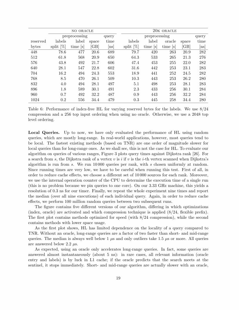
no oracle 20k oraclepreprocessing query preprocessing query

reserved labels label space time labels label oracle space timebytes split [%] time [s] [GB] [ns] split [%] time [s] time [s] [GB] [ns]448 78.6 477 20.6 689 79.7 420 263 20.9 282512 61.8 568 20.9 650 64.3 533 265 21.3 276576 43.8 492 21.7 606 47.4 453 255 22.0 282640 28.1 547 22.8 602 31.6 442 253 23.1 283704 16.2 494 24.3 553 18.9 441 252 24.5 282768 8.5 470 26.1 509 10.3 443 253 26.2 280832 4.0 494 28.1 497 5.1 498 253 28.1 283896 1.8 589 30.1 491 2.3 433 256 30.1 284960 0.7 492 32.2 487 0.9 443 256 32.2 2841024 0.2 556 34.4 479 0.3 445 258 34.4 280

Table 6: Performance of index-free HL for varying reserved bytes for the labels. We use 8/24compression and a 256 top input ordering when using no oracle. Otherwise, we use a 2048 toplevel ordering.

Local Queries. Up to now, we have only evaluated the performance of HL using randomqueries, which are mostly long-range. In real-world applications, however, most queries tend tobe local. The fastest existing methods (based on TNR) are one order of magnitude slower forlocal queries than for long-range ones. As we shall see, this is not the case for HL. To evaluate ouralgorithm on queries of various ranges, Figure 3 plots query times against Dijkstra rank [26]. Fora search from s, the Dijkstra rank of a vertex v is i if v is the i-th vertex scanned when Dijkstra’salgorithm is run from s. We run 10 000 queries per rank, with s chosen uniformly at random.Since running times are very low, we have to be careful when running this test. First of all, inorder to reduce cache effects, we choose a different set of 10 000 sources for each rank. Moreover,we use the internal operation counter of the CPU to determine the execution time of a single run(this is no problem because we pin queries to one core). On our 3.33 GHz machine, this yields aresolution of 0.3 ns for our timer. Finally, we repeat the whole experiment nine times and reportthe median (over all nine executions) of each individual query. Again, in order to reduce cacheeffects, we perform 100 million random queries between two subsequent runs.

The figure contains five different versions of our algorithm, differing in which optimizations(index, oracle) are activated and which compression technique is applied (8/24, flexible prefix).The first plot contains methods optimized for speed (with 8/24 compression), while the secondcontains methods with lower space usage.

As the first plot shows, HL has limited dependence on the locality of a query compared toTNR. Without an oracle, long-range queries are a factor of two faster than short- and mid-rangequeries. The median is always well below 1 µs and only outliers take 1.5 µs or more. All queriesare answered below 2.2 µs.

As expected, using an oracle only accelerates long-range queries. In fact, some queries areanswered almost instantaneously (about 5 ns): in rare cases, all relevant information (oracleentry and labels) is by luck in L1 cache; if the oracle predicts that the search meets at thesentinel, it stops immediately. Short- and mid-range queries are actually slower with an oracle,

19

due to the different label ordering (top 2048 level with oracle, top 256 input without). Moreover,accessing the oracle array can be (relatively) costly. Removing the index slows down short-rangequeries even more, since these queries tend to access the escape array.

Comparing both plots, we observe that using flexible prefix instead of 8/24 compression slowsdown queries by about 500 ns, independent of the Dijkstra rank. Still, all queries are answeredin less than 3 µs. Interestingly, with prefix compression and no oracle, query times are almostindependent of the Dijkstra rank: Since we use inverted ranks to set the internal IDs, both labelsare traversed almost to the end on all queries.

To summarize, the index-free version with partition oracle is the best choice for long-rangequeries, with local queries four to five times slower. The version with index and without partitionoracle is the fastest for local queries; it has almost the same performance for all query types.

6.2 Comparison with Existing Algorithms

In this section we compare HL to five previously known fast algorithms. The first one, CH [16],has been discussed in Section 3. The second algorithm, CHASE, is a combination of CH and arcflags [6].

The third algorithm is High-Performance Multi-Level Routing (HPML) [11]. This is the fastestprevious algorithm for local queries. During preprocessing, it computes a hierarchy of graphseparators, and uses it to compute and store many small (sparsified) graphs. Level graphs encodethe distances between separators of a component on the same level, while upward (downward)graphs store the distances between separators and more (less) important separators in the samecomponent. The query algorithm of HPML first connects the appropriate sequence of small graphsand then performs a (linear-time) search on the resulting graph. While the preprocessing is verytime-consuming, this was the first approach to handle random queries in a matter of tens ofmicroseconds. Unfortunately, the published implementation does not support very local queries.

The next algorithm in our study is transit node routing (TNR), introduced in [3]. As alreadymentioned, this approach uses a distance table to answer long-range queries very efficiently. Foreach vertex u, TNR preprocessing computes its access nodes, a set of nodes that covers all suf-ficiently long shortest paths starting or ending at u. Moreover, the distances between u and itsaccess nodes are precomputed. Finally, a full distance table between all access nodes (collectivelyknown as transit nodes) is computed and stored. On a continent-size road network, one can pickaround 10 000 transit nodes such that each vertex has less than 10 access nodes on average.

The query algorithm uses a Euclidean-based locality filter to determine if a query is local orglobal. Local queries are handled by a Dijkstra-based algorithm (CH in the fastest version [16]).For a global s–t query, the shortest path contains an access node of s and one of t. Therefore, thequery examines all pairs x, y where x and y are access nodes of s and t, respectively, and finds apair that minimizes d(s, x) + d(x, y) + d(y, t).

Long-range queries are dominated by distance table lookups, of which there are less than 100on average. This is significantly faster than a typical local query implemented by CH. The mostefficient version of TNR introduces several layers of transit nodes to accelerate mid-range queries.

The last algorithm we consider is the combination of TNR and arc flags (TNR+AF) [6]. Arcflags reduce the average number of table lookups by an order of magnitude, to less than four [6],making this the fastest previously known algorithm for random queries.

We compare these algorithms with three variants of HL, chosen based on the experiments

20

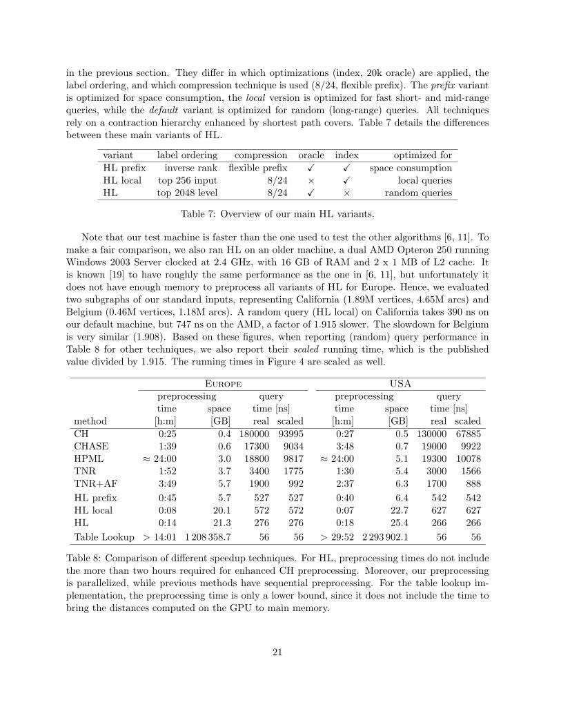
in the previous section. They differ in which optimizations (index, 20k oracle) are applied, thelabel ordering, and which compression technique is used (8/24, flexible prefix). The prefix variantis optimized for space consumption, the local version is optimized for fast short- and mid-rangequeries, while the default variant is optimized for random (long-range) queries. All techniquesrely on a contraction hierarchy enhanced by shortest path covers. Table 7 details the differencesbetween these main variants of HL.

variant label ordering compression oracle index optimized forHL prefix inverse rank flexible prefix X X space consumptionHL local top 256 input 8/24 × X local queriesHL top 2048 level 8/24 X × random queries

Table 7: Overview of our main HL variants.

Note that our test machine is faster than the one used to test the other algorithms [6, 11]. Tomake a fair comparison, we also ran HL on an older machine, a dual AMD Opteron 250 runningWindows 2003 Server clocked at 2.4 GHz, with 16 GB of RAM and 2 x 1 MB of L2 cache. Itis known [19] to have roughly the same performance as the one in [6, 11], but unfortunately itdoes not have enough memory to preprocess all variants of HL for Europe. Hence, we evaluatedtwo subgraphs of our standard inputs, representing California (1.89M vertices, 4.65M arcs) andBelgium (0.46M vertices, 1.18M arcs). A random query (HL local) on California takes 390 ns onour default machine, but 747 ns on the AMD, a factor of 1.915 slower. The slowdown for Belgiumis very similar (1.908). Based on these figures, when reporting (random) query performance inTable 8 for other techniques, we also report their scaled running time, which is the publishedvalue divided by 1.915. The running times in Figure 4 are scaled as well.

Europe USApreprocessing query preprocessing querytime space time [ns] time space time [ns]

method [h:m] [GB] real scaled [h:m] [GB] real scaledCH 0:25 0.4 180000 93995 0:27 0.5 130000 67885CHASE 1:39 0.6 17300 9034 3:48 0.7 19000 9922HPML ≈ 24:00 3.0 18800 9817 ≈ 24:00 5.1 19300 10078TNR 1:52 3.7 3400 1775 1:30 5.4 3000 1566TNR+AF 3:49 5.7 1900 992 2:37 6.3 1700 888HL prefix 0:45 5.7 527 527 0:40 6.4 542 542HL local 0:08 20.1 572 572 0:07 22.7 627 627HL 0:14 21.3 276 276 0:18 25.4 266 266Table Lookup > 14:01 1 208 358.7 56 56 > 29:52 2 293 902.1 56 56

Table 8: Comparison of different speedup techniques. For HL, preprocessing times do not includethe more than two hours required for enhanced CH preprocessing. Moreover, our preprocessingis parallelized, while previous methods have sequential preprocessing. For the table lookup im-plementation, the preprocessing time is only a lower bound, since it does not include the time tobring the distances computed on the GPU to main memory.

21

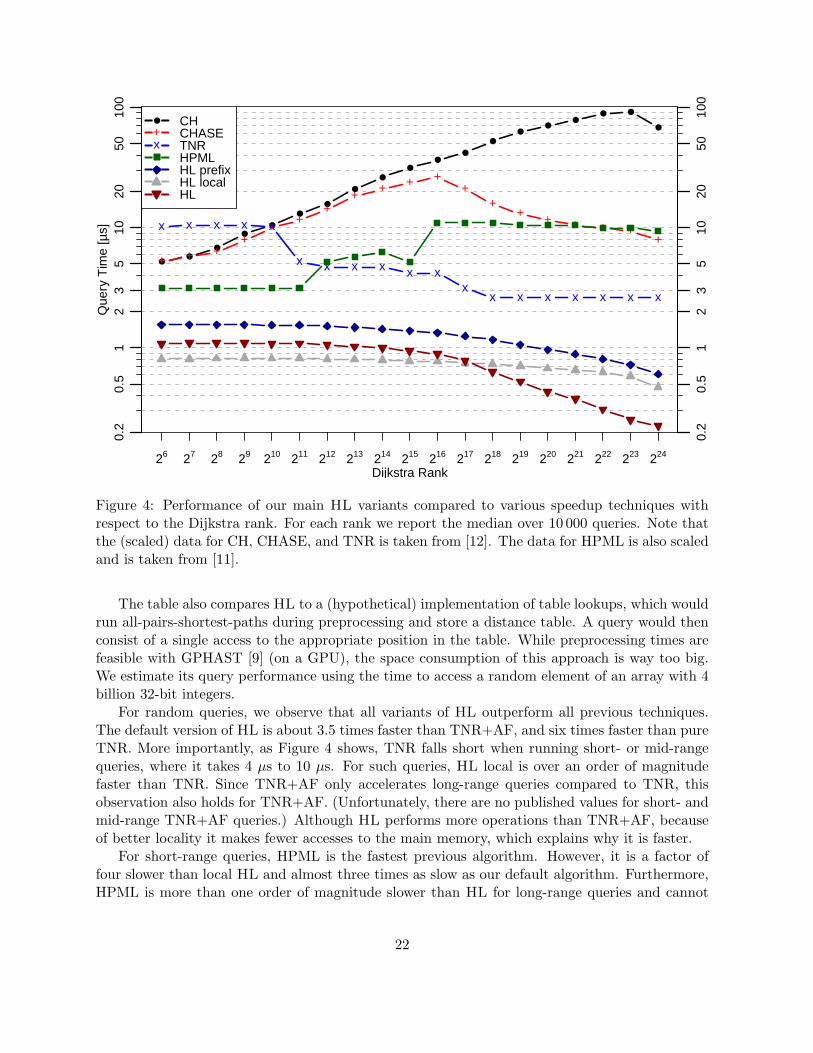
Dijkstra Rank

Que

ry T

ime

[µs]

26 27 28 29 210 211 212 213 214 215 216 217 218 219 220 221 222 223 224

0.2

0.5

12

35

1020

5010

0

0.2

0.5

12

35

1020

5010

0

●

+x

CHCHASETNRHPMLHL prefixHL localHL

●●

●

●●

●●

●

●●

●●

●●

●●

● ●

●

+ + ++

++

++ + + +

++

+ + + + ++

x x x x x

x x x x x xx

x x x x x x x

Figure 4: Performance of our main HL variants compared to various speedup techniques withrespect to the Dijkstra rank. For each rank we report the median over 10 000 queries. Note thatthe (scaled) data for CH, CHASE, and TNR is taken from [12]. The data for HPML is also scaledand is taken from [11].

The table also compares HL to a (hypothetical) implementation of table lookups, which wouldrun all-pairs-shortest-paths during preprocessing and store a distance table. A query would thenconsist of a single access to the appropriate position in the table. While preprocessing times arefeasible with GPHAST [9] (on a GPU), the space consumption of this approach is way too big.We estimate its query performance using the time to access a random element of an array with 4billion 32-bit integers.

For random queries, we observe that all variants of HL outperform all previous techniques.The default version of HL is about 3.5 times faster than TNR+AF, and six times faster than pureTNR. More importantly, as Figure 4 shows, TNR falls short when running short- or mid-rangequeries, where it takes 4 µs to 10 µs. For such queries, HL local is over an order of magnitudefaster than TNR. Since TNR+AF only accelerates long-range queries compared to TNR, thisobservation also holds for TNR+AF. (Unfortunately, there are no published values for short- andmid-range TNR+AF queries.) Although HL performs more operations than TNR+AF, becauseof better locality it makes fewer accesses to the main memory, which explains why it is faster.

For short-range queries, HPML is the fastest previous algorithm. However, it is a factor offour slower than local HL and almost three times as slow as our default algorithm. Furthermore,HPML is more than one order of magnitude slower than HL for long-range queries and cannot

22

handle some short-range queries at all.We also observe that compression succeeds; for Europe, HL prefix has roughly a four times

lower space consumption than HL but is only twice as slow (for all types of queries). Even so,this version outperforms TNR+AF as well.

Comparing HL to a hypothetical table lookup implementation, we observe that the spaceconsumption of HL is 56 730 (Europe) to 90 311 (USA) times lower, and it has much more practicalpreprocessing times. Still, random queries are only five times slower. In other words, with ouroptimizations a random HL query is as fast as five random accesses to main memory. For short-and mid-range queries, however, HL local is about 13 times slower than a random access.

7 Concluding Remarks

We have presented an efficient implementation of Hub Labels (HL), the algorithm with the besttheoretical bounds among those studied by Abraham et al. [1]. We have demonstrated that HL ispractical; in fact, it is the fastest known speedup technique for computing point-to-point distanceson road networks. Although ours is not a strict implementation of the theoretical algorithm, itmakes use of shortest path covers (the basis of the theoretical analysis) to obtain additionalspeedups.

In addition to an efficient implementation of the basic algorithm, we introduced two labelcompression techniques, a distance oracle to accelerate long-range (and random) queries, and theindex-free variant of the algorithm. These techniques can be combined, resulting in many variantsof HL. Three variants are the most interesting ones. The variant with index, no distance oracle,and 8/24 compression is simple and the fastest on local queries. Our default variant, which addsdistance oracles and is index-free, is the fastest on random queries, a convenient benchmark thatis used extensively in the literature. Adding prefix compression decreases the space requirementsof our algorithm at the expense of the running time. The resulting algorithm uses as much spaceas TNR+AF, but is still faster on random queries and an order of magnitude faster on localqueries.

Due to the excellent query performance, it is often feasible to run many point-to-point HLqueries to solve basic problems in road networks. For example, for our Europe instance, a veryefficient implementation of Dijkstra’s algorithm [17] needs 2.21 seconds to compute the distancesfrom one vertex to all others. Computing these distances with HL takes only 0.93 seconds. Notethat we need less time per entry (51.8 ns) than random queries do, since the forward label of theroot vertex stays in L1 cache and reverse labels are traversed sequentially. Another advantageof running HL queries instead of Dijkstra’s algorithm is its easy parallelization. However, HLcannot catch up with PHAST [9], which needs less than 1 ns per distance entry.

We note that some of the ideas presented in this paper could probably be used to accelerateother techniques as well. In particular, a variant of our partition oracle could be used withintransit node routing as a locality filter. During preprocessing, we first partition the graph into kregions. We then create a k × k boolean matrix in which entry (A,B) is true iff every s–t querywith s ∈ A to t ∈ B is global, i.e., if it can be solved using transit nodes. To build this table, weneed to run queries among the boundary vertices and external access nodes of all regions.

Finding better shortest path cover algorithms is an interesting research topic. On the theoreti-cal side, we have a recent (unpublished) result showing how to improve the approximation boundsof [1] using an algorithm for finding hitting sets in low VC-dimension [7]. On the practical side,

23

it may be possible to improve the speed or the quality of cover computations, which could leadto smaller labels. A sufficiently fast algorithm may allow CH preprocessing based exclusively onshortest paths covers, which could lead to a better CH ordering. Similarly, computing HL labelsbased exclusively on shortest path covers is an obvious research direction. We expect that im-proved SPC algorithms and better orderings will have a positive effect on the query performanceof HL.

Of course, it is also interesting to improve HL itself. Further improvements in speed arealways desirable, but a more practical goal would be to further reduce the space usage of ouralgorithms. One could also think of how HL can be adapted to work in augmented scenarios liketime-dependent networks or multi-criteria optimization. Memory consumption is again an issue,but compression and approximation techniques may help.

Another interesting question is minimizing the average label size. One can ask for both upperand lower bounds, both experimental and theoretical. On the theoretical size, the problem offinding the optimal labeling is probably NP-hard, but it is unclear whether a constant-factorapproximation can be obtained in polynomial time.

References

[1] I. Abraham, A. Fiat, A. V. Goldberg, and R. F. Werneck. Highway Dimension, Shortest Paths, andProvably Efficient Algorithms. In Proceedings of the 21st Annual ACM–SIAM Symposium on DiscreteAlgorithms (SODA’10), pages 782–793, 2010.

[2] G. Ausiello, P. Crescenzi, G. Gambosi, V. Kann, and A. Marchetti-Spaccamela. Complexity and Ap-proximation - Combinatorial Optimization Problems and Their Approximability Properties. Springer,second edition, 2002.

[3] H. Bast, S. Funke, D. Matijevic, P. Sanders, and D. Schultes. In Transit to Constant Shortest-Path Queries in Road Networks. In Proceedings of the 9th Workshop on Algorithm Engineering andExperiments (ALENEX’07), pages 46–59. SIAM, 2007.

[4] H. Bast, S. Funke, P. Sanders, and D. Schultes. Fast Routing in Road Networks with Transit Nodes.Science, 316(5824):566, 2007.

[5] R. Bauer and D. Delling. SHARC: Fast and Robust Unidirectional Routing. ACM Journal of Exper-imental Algorithmics, 14(2.4):1–29, August 2009. Special Section on Selected Papers from ALENEX2008.

[6] R. Bauer, D. Delling, P. Sanders, D. Schieferdecker, D. Schultes, and D. Wagner. Combining Hierarchi-cal and Goal-Directed Speed-Up Techniques for Dijkstra’s Algorithm. ACM Journal of ExperimentalAlgorithmics, 15(2.3):1–31, January 2010. Special Section devoted to WEA’08.

[7] H. Bronnimann and M. Goodrich. Almost Optimal Set Covers in Finite VC-dimension. Discrete andComputational Geometry, 14:463–497, 1995.

[8] G. B. Dantzig. Linear Programming and Extensions. Princeton Univ. Press, Princeton, NJ, 1962.

[9] D. Delling, A. V. Goldberg, A. Nowatzyk, and R. F. Werneck. PHAST: Hardware-Accelerated ShortestPath Trees. Technical Report MSR-TR-2010-125, Microsoft Research, 2010.

[10] D. Delling, A. V. Goldberg, I. Razenshteyn, and R. F. Werneck. Graph Partitioning with NaturalCuts. Technical Report MSR-TR-2010-164, Microsoft Research, 2010.

24

[11] D. Delling, M. Holzer, K. Muller, F. Schulz, and D. Wagner. High-Performance Multi-Level Routing.In C. Demetrescu, A. V. Goldberg, and D. S. Johnson, editors, The Shortest Path Problem: Ninth DI-MACS Implementation Challenge, volume 74 of DIMACS Book, pages 73–92. American MathematicalSociety, 2009.

[12] D. Delling, P. Sanders, D. Schultes, and D. Wagner. Engineering Route Planning Algorithms. InJ. Lerner, D. Wagner, and K. Zweig, editors, Algorithmics of Large and Complex Networks, volume5515 of LNCS, pages 117–139. Springer, 2009.

[13] C. Demetrescu, A. V. Goldberg, and D. S. Johnson, editors. 9th DIMACS Implementation Challenge- Shortest Paths, 2006.

[14] E. W. Dijkstra. A Note on Two Problems in Connexion with Graphs. Numer. Math., 1:269–271, 1959.

[15] C. Gavoille, D. Peleg, S. Perennes, and R. Raz. Distance labeling in graphs. J. Algorithms, 53(1):85–112, 2004.

[16] R. Geisberger, P. Sanders, D. Schultes, and D. Delling. Contraction Hierarchies: Faster and SimplerHierarchical Routing in Road Networks. In C. C. McGeoch, editor, Proceedings of the 7th InternationalWorkshop on Experimental Algorithms (WEA’08), volume 5038 of LNCS, pages 319–333. Springer,June 2008.

[17] A. V. Goldberg. A Practical Shortest Path Algorithm with Linear Expected Time. SIAM J. Comput.,37:1637–1655, 2008.

[18] A. V. Goldberg and C. Harrelson. Computing the Shortest Path: A∗ Search Meets Graph Theory. InProc. 16th ACM-SIAM Symposium on Discrete Algorithms, pages 156–165, 2005.

[19] A. V. Goldberg, H. Kaplan, and R. F. Werneck. Reach for A*: Shortest Path Algorithms withPreprocessing. In C. Demetrescu, A. V. Goldberg, and D. S. Johnson, editors, The Shortest PathProblem: Ninth DIMACS Implementation Challenge, volume 74 of DIMACS Book, pages 93–139.American Mathematical Society, 2009.

[20] R. Gutman. Reach-based Routing: A New Approach to Shortest Path Algorithms Optimized for RoadNetworks. In Proc. 6th International Workshop on Algorithm Engineering and Experiments, pages100–111, 2004.

[21] M. Hilger, E. Kohler, R. H. Mohring, and H. Schilling. Fast Point-to-Point Shortest Path Computationswith Arc-Flags. In C. Demetrescu, A. Goldberg, and D. Johnson, editors, The Shortest Path Problem:Ninth DIMACS Implementation Challenge, pages 73–92. AMS, 2009.

[22] S. Knopp, P. Sanders, D. Schultes, F. Schulz, and D. Wagner. Computing Many-to-Many ShortestPaths Using Highway Hierarchies. In Proceedings of the 9th Workshop on Algorithm Engineering andExperiments (ALENEX’07), pages 36–45, 2007.

[23] U. Lauther. An Extremely Fast, Exact Algorithm for Finding Shortest Paths in Static Networkswith Geographical Background. In IfGIprints 22, Institut fuer Geoinformatik, Universitaet Muenster(ISBN 3-936616-22-1), pages 219–230, 2004.

[24] PTV AG - Planung Transport Verkehr. http://www.ptv.de.

[25] M. Resende and R. F. Werneck. A Fast Swap-based Local Search Procedure for Location Problems.Annals of Operations Research, 150:205–230, 2007.

[26] P. Sanders and D. Schultes. Highway Hierarchies Hasten Exact Shortest Path Queries. In Proceedingsof the 13th Annual European Symposium on Algorithms (ESA’05), volume 3669 of Lecture Notes inComputer Science, pages 568–579. Springer, 2005.

25

[27] P. Sanders and D. Schultes. Engineering Highway Hierarchies. In Proceedings of the 14th AnnualEuropean Symposium on Algorithms (ESA’06), volume 4168 of Lecture Notes in Computer Science,pages 804–816. Springer, 2006.

[28] D. Schultes and P. Sanders. Dynamic Highway-Node Routing. In C. Demetrescu, editor, Proceedings ofthe 6th Workshop on Experimental Algorithms (WEA’07), volume 4525 of Lecture Notes in ComputerScience, pages 66–79. Springer, June 2007.

[29] R. E. Tarjan. Data Structures and Network Algorithms. Society for Industrial and Applied Mathe-matics, Philadelphia, PA, 1983.

[30] M. Thorup and U. Zwick. Approximate distance oracles. J. Assoc. Comput. Mach., 52(1):1–24, 2005.

[31] D. US Census Bureau, Washington. UA Census 2000 TIGER/Line files.http://www.census.gov/geo/www/tiger/tigerua/ua.tgr2k.html, 2002.

26