a guide to climate change and adaptation in agriculture · pdf filelikely impacts of climate...
TRANSCRIPT
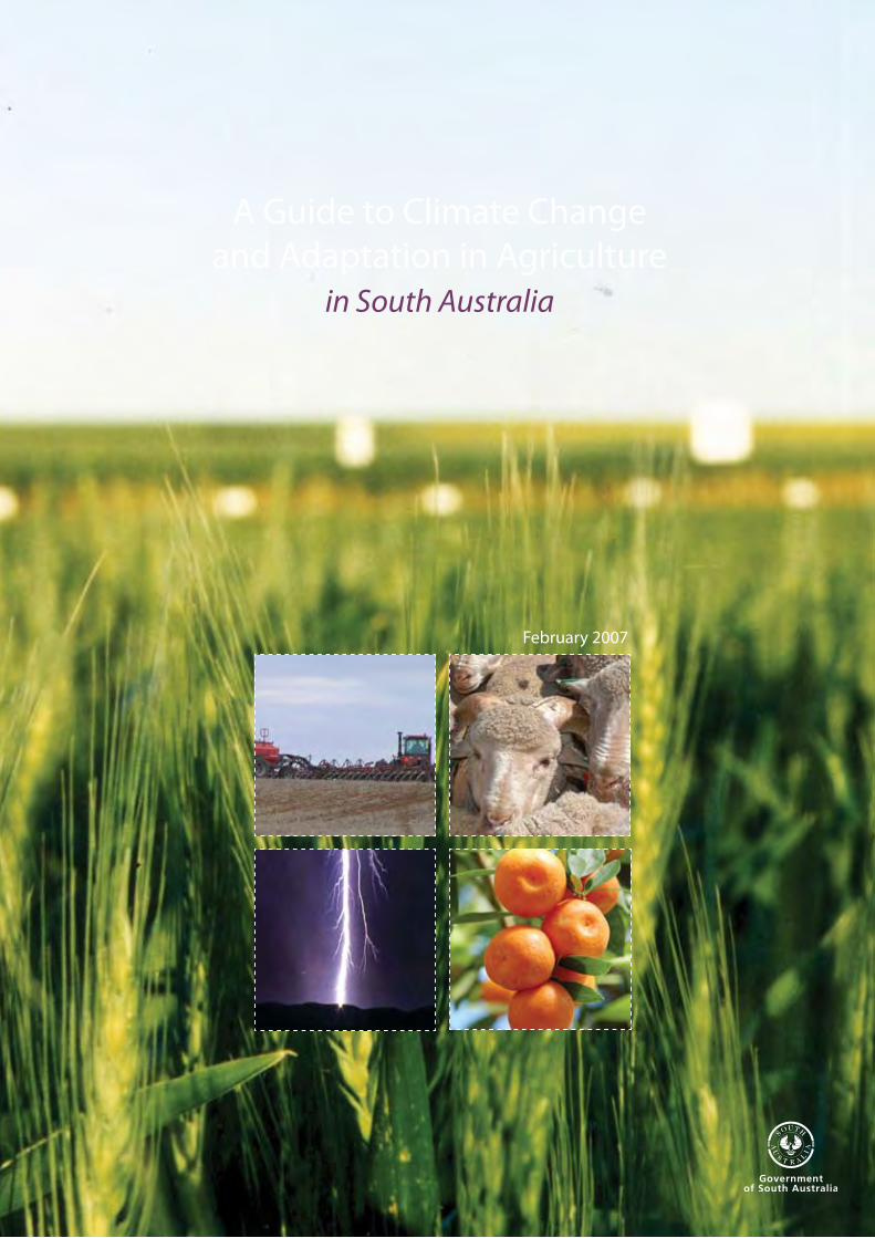
A Guide to Climate Change and Adaptation in Agriculture
in South Australia
February 2007
Edited by: Leona Coleman
Layout and design by: PIRSA Publishing Services
ISBN 978-0-7590-1397-1
Disclaimer
Primary Industries and Resources SA, Rural Solutions SA and South Australian Research and Development Institute and their employees do not warrant or make any representation regarding the use, or results of the use, of the information contained herein as regards to its correctness, accuracy, reliability, currency or otherwise. Primary Industries and Resources SA and Rural Solutions SA and their employees expressly disclaim all liability or responsibility to any person using the information or advice.
© South Australian Research and Development Institute, Primary Industries and Resources SA and Rural Solutions SA
This work is copyright. Unless permitted under the Copyright Act 1968 (Cwlth), no part may be reproduced by any process without prior written permission from SARDI, PIRSA or Rural Solutions SA.
We would like to gratefully acknowledge:
Funding support from South Australian Grains Industry Trust (SAGIT) to develop this guide.
Technical input from Dr Peter Hayman — SARDI Climate Applications.
Technical input from Dr Beth Curran — SA Bureau of Meteorology.
Initial layout and input by Trudi Duffield — SARDI Climate Applications.
•
•
•
•
Acknowledgements
Supported by: Rural Solutions SA
PIRSA Publishing Services_203250
Melissa Rebbeck South Australian Research and Development Institute
Elliot Dwyer Primary Industries and Resources SA
Mark Bartetzko and Amy Williams Rural Solutions SA
February 2007
A Guide to Climate Change and Adaptation in Agriculture
in South Australia
A Guide to Climate Change and Adaptation in Agriculture South Australia
Introduction . . . . . . . . . . . . . . . . . . . . . . . . . . . . . . . . . . . . . . . . . . . . . . . . . . . . . . . . . . 4
Planning for climate change . . . . . . . . . . . . . . . . . . . . . . . . . . . . . . . . . . . . . . . . . . . 4
In this guide . . . . . . . . . . . . . . . . . . . . . . . . . . . . . . . . . . . . . . . . . . . . . . . . . . . . . . . . . . 4
The future . . . . . . . . . . . . . . . . . . . . . . . . . . . . . . . . . . . . . . . . . . . . . . . . . . . . . . . . . . . . 5
1 . Greenhouse emissions and global warming . . . . . . . . . . . . . . . . . . . . . . . . . . 6
Fourth Assessment Report of the Intergovernmental Panel on Climate Change . . . . . . . . . . . . . . . . . . . . . . . . . . . . . . . . . . . . . . . . . . . . . . . . . . . 6
Reasons for uncertainty in climate change projections . . . . . . . . . . . . . . . . . 8
What is the greenhouse effect? . . . . . . . . . . . . . . . . . . . . . . . . . . . . . . . . . . . . . . . . 8
Greenhouse gases . . . . . . . . . . . . . . . . . . . . . . . . . . . . . . . . . . . . . . . . . . . . . . . . . . . . 9
Agricultural greenhouse gas emissions . . . . . . . . . . . . . . . . . . . . . . . . . . . . . . . 10
Carbon sequestration . . . . . . . . . . . . . . . . . . . . . . . . . . . . . . . . . . . . . . . . . . . . . . . . 11
Trends in agricultural emissions and sinks . . . . . . . . . . . . . . . . . . . . . . . . . . . . . 11
2 . Climate change trends . . . . . . . . . . . . . . . . . . . . . . . . . . . . . . . . . . . . . . . . . . . .12
Climate change trends . . . . . . . . . . . . . . . . . . . . . . . . . . . . . . . . . . . . . . . . . . . . . . . 12
Temperature trends . . . . . . . . . . . . . . . . . . . . . . . . . . . . . . . . . . . . . . . . . . . . . . . . . . 12
Rainfall trends . . . . . . . . . . . . . . . . . . . . . . . . . . . . . . . . . . . . . . . . . . . . . . . . . . . . . . . 13
Evaporation trends . . . . . . . . . . . . . . . . . . . . . . . . . . . . . . . . . . . . . . . . . . . . . . . . . . . 14
3 . Climate change projections . . . . . . . . . . . . . . . . . . . . . . . . . . . . . . . . . . . . . . . .15
Climate change projections . . . . . . . . . . . . . . . . . . . . . . . . . . . . . . . . . . . . . . . . . . 15
Temperature change projections . . . . . . . . . . . . . . . . . . . . . . . . . . . . . . . . . . . . . 15
Rainfall change projections . . . . . . . . . . . . . . . . . . . . . . . . . . . . . . . . . . . . . . . . . . . 17
Water balance and evaporation projections . . . . . . . . . . . . . . . . . . . . . . . . . . . 19
Extreme events projections . . . . . . . . . . . . . . . . . . . . . . . . . . . . . . . . . . . . . . . . . . . 19
Extreme events at the coast . . . . . . . . . . . . . . . . . . . . . . . . . . . . . . . . . . . . . . . . . . 19
4 . Climate change impacts on agriculture . . . . . . . . . . . . . . . . . . . . . . . . . . . . .20
Likely impacts of climate change on agriculture . . . . . . . . . . . . . . . . . . . . . . . 20
Temperature impacts . . . . . . . . . . . . . . . . . . . . . . . . . . . . . . . . . . . . . . . . . . . . . . . . 20
Rainfall/water supply impacts . . . . . . . . . . . . . . . . . . . . . . . . . . . . . . . . . . . . . . . . 20
Contents
A Guide to Climate Change and Adaptation in Agriculture South Australia
Extreme events . . . . . . . . . . . . . . . . . . . . . . . . . . . . . . . . . . . . . . . . . . . . . . . . . . . . . . 20
Coastal impacts . . . . . . . . . . . . . . . . . . . . . . . . . . . . . . . . . . . . . . . . . . . . . . . . . . . . . . 20
Goyder’s line . . . . . . . . . . . . . . . . . . . . . . . . . . . . . . . . . . . . . . . . . . . . . . . . . . . . . . . . . 21
Ecosystem impacts . . . . . . . . . . . . . . . . . . . . . . . . . . . . . . . . . . . . . . . . . . . . . . . . . . . 21
Trade impacts . . . . . . . . . . . . . . . . . . . . . . . . . . . . . . . . . . . . . . . . . . . . . . . . . . . . . . . . 21
Vulnerability . . . . . . . . . . . . . . . . . . . . . . . . . . . . . . . . . . . . . . . . . . . . . . . . . . . . . . . . . 21
Websites for more information . . . . . . . . . . . . . . . . . . . . . . . . . . . . . . . . . . . . . . . 21
5 . Climate change mitigation and adaptation in agriculture . . . . . . . . . . . .22
Strategies for reducing greenhouse gas emissions . . . . . . . . . . . . . . . . . . . . 22
Adaptation in agriculture . . . . . . . . . . . . . . . . . . . . . . . . . . . . . . . . . . . . . . . . . . . . . 23
Adaptive capacity . . . . . . . . . . . . . . . . . . . . . . . . . . . . . . . . . . . . . . . . . . . . . . . . . . . . 23
Levels of treatment . . . . . . . . . . . . . . . . . . . . . . . . . . . . . . . . . . . . . . . . . . . . . . . . . . . 23
Priority scoring of climate risks . . . . . . . . . . . . . . . . . . . . . . . . . . . . . . . . . . . . . . . 24
Short term adaptive measures . . . . . . . . . . . . . . . . . . . . . . . . . . . . . . . . . . . . . . . . 24
Longer term adaptive measures . . . . . . . . . . . . . . . . . . . . . . . . . . . . . . . . . . . . . . 25
Further considerations . . . . . . . . . . . . . . . . . . . . . . . . . . . . . . . . . . . . . . . . . . . . . . . 26
6 . Future considerations . . . . . . . . . . . . . . . . . . . . . . . . . . . . . . . . . . . . . . . . . . . . .28
Monitoring . . . . . . . . . . . . . . . . . . . . . . . . . . . . . . . . . . . . . . . . . . . . . . . . . . . . . . . . . . 28
Review . . . . . . . . . . . . . . . . . . . . . . . . . . . . . . . . . . . . . . . . . . . . . . . . . . . . . . . . . . . . . . 38
References and futher reading . . . . . . . . . . . . . . . . . . . . . . . . . . . . . . . . . . . . . . . .29
References . . . . . . . . . . . . . . . . . . . . . . . . . . . . . . . . . . . . . . . . . . . . . . . . . . . . . . . . . . . 29
Further reading . . . . . . . . . . . . . . . . . . . . . . . . . . . . . . . . . . . . . . . . . . . . . . . . . . . . . . 30
Appendix 1 — Carbon dioxide concentration in the atmosphere over 400 000 years . . . . . . . . . . . . . . . . . . . . . . . . . . . . . . . . . . . . . . . . . . . . . . . . . . . .31
Appendix 2 — History of International and Australian policy of climate change . . . . . . . . . . . . . . . . . . . . . . . . . . . . . . . . . . . . . . . . . . . . . . . . . . . . .32
Policy timeline . . . . . . . . . . . . . . . . . . . . . . . . . . . . . . . . . . . . . . . . . . . . . . . . . . . . . . . 32
The Kyoto Protocol . . . . . . . . . . . . . . . . . . . . . . . . . . . . . . . . . . . . . . . . . . . . . . . . . . . 33
A potential greenhouse gas emission trading scheme . . . . . . . . . . . . . . . . . 33
A Guide to Climate Change and Adaptation in Agriculture South Australia4
Introduction
There is significant pressure on primary producers in South Australia . Production can vary considerably from one year to the next due to climate . For example, in low rainfall grain producing regions, 80% of the profit is typically made from the best three years in ten, while a loss is often the result from the worst three years in ten . This is reflected in the recent grain harvests in South Australia . Our worst cereal harvest in decades was just 2 .9 million tonnes in 2006–07, compared with our best ever of 9 .3 million tonnes in 2001–02 .
It has been a key challenge for producers to assess if a good or bad year is likely so they can maximise profits in the good years and minimise losses in the bad . This challenge is exacerbated by uncertainty about how climate extremes and average conditions will change as a result of climate change .
The demand for our agricultural exports has generally increased over the last two decades with increasing demand for food internationally . Currently the global population is around six billion and it is expected to grow to around nine billion by 2020 . The demand for food will therefore increase, with export of cereals and meat expected to double by 2020 (22) . Furthermore, farms today are fewer and larger than 20 years ago, perhaps partially due to climate variability, but also due to the pursuit of economies of scale as a means of decreasing costs (18) .
Considering all of these factors, primary producers need to know how to best adapt the management of their agricultural enterprises for climate variability, whilst factoring in long term climate . It is not just the average projected long-term change that is of concern; understanding and adapting to changing climate extremes is a major issue .
Recently many organisations have become aware of the issue of climate change . However, once farmers have been convinced that climate change is real, there has been little information about what they can do to adapt to this change .
This guide presents a systematic approach to risk management that attempts to remedy this situation .
Planning for climate change
Two aspects of managing the risks to agriculture associated with our variable and changing climate are considered within this guide:
Managing for short term climate variability and change
Managing for change in the longer term .
Farmers have always had to cope with variability between seasons, but now, greater extremes in seasonal variation are projected . In these circumstances, seasonal forecasts will become even more important for managers who need
to make decisions about the balance of their activities . Examples of responses to advance warning of seasonal conditions might include changes in the area sown to crops, modifications to stocking rates or variation of fodder conservation and utilisation strategies .
Farmers will also need to assess their current enterprises in light of the threats posed by climate change in the longer term . The responses of managers to projected trends may go as far as a change in the nature of the enterprise . For example, a change from cropping to livestock might be required as seasonal conditions for reliable cropping decline .
The procedures used in assessment, planning and response to change are known as risk management .
In this Guide
This guide will help you to better plan for short and longer term climate change challenges and opportunities in agriculture by providing you with a simplified background on
Greenhouse emissions
Climate change trends
Climate change projections
Climate change impacts on agriculture
Climate change mitigation and adaptation in agriculture .
A Guide to Climate Change and Adaptation in Agriculture South Australia 5
The Future
Scientific knowledge and understanding of climate change is developing rapidly . So too, is our awareness of the impacts and consequences of climate change on our farms and, of course, on other areas of our lives and businesses . Further details are provided in the references and reading list at the back of the Guide, particularly the CSIRO Report by Suppiah and others (6) . The Australian Greenhouse Office, Canberra, is especially useful with information and advice in printed publications and on-line at www .greenhouse .gov .au/agriculture/index .html .
Chapter ONE
1
A Guide to Climate Change and Adaptation in Agriculture South Australia6
Greenhouse emissions and global warming
Fourth Assessment Report of the Intergovernmental Panel on Climate Change (26)
The International Panel on Climate Change (IPCC) is an organisation that brings together scientific work from more than 2000 climate change scientists from around the world and each six years releases assessment reports summarising the scientific consensus . The IPCC released Volume 1 of its Fourth Assessment Report (AR4) on 2nd February 2007 (26), confirming many of the projections of the Third Assessment Report in 2001:
Global atmospheric concentrations of carbon dioxide, methane and nitrous oxide have increased markedly as a result of human activities since 1750 and now far exceed pre-industrial values determined from ice cores spanning many thousands of years . The global increases in carbon dioxide concentration are due primarily to fossil fuel use and land-use change, while those of methane and nitrous oxide are primarily due to agriculture .
The understanding of anthropogenic warming and cooling influences on climate has improved since the Third Assessment Report (TAR), leading to very high confidence that the globally averaged net effect of human activities since 1750 has been one of warming, with a radiative forcing * of +1 .6 [+0 .6 to +2 .4] W/m2 . * Note: Radiative forcing is a measure of the influence that a factor has in altering the balance of incoming
and outgoing energy in the Earth-atmosphere system and is an index of the importance of the factor as a potential climate change mechanism . Positive forcing tends to warm the surface while negative forcing tends to cool it . In this report radiative forcing values are for 2005 relative to pre-industrial conditions defined at 1750 and are expressed in watts per square metre (W/m2) .
Warming of the climate system is unequivocal, as is now evident from observations of increases in global average air and ocean temperatures, widespread melting of snow and ice, and rising global average sea level .
Eleven of the last twelve years (1995 –2006) rank among the 12 warmest years in the instrumental record of global surface temperature (since 1850) . The linear warming trend over the last 50 years (0 .13 [0 .10 to 0 .16] °C per decade) is nearly twice that for the last 100 years . The total temperature increase from 1850–1899 to 2001–2005 is 0 .76 [0 .57 to 0 .95] °C .
The average atmospheric water vapour content has increased since at least the 1980s over land and ocean as well as in the upper troposphere . The increase is broadly consistent with the extra water vapour that warmer air can hold .
Observations since 1961 show that the average temperature of the global ocean has increased to depths of
−
−
−
at least 3000 m and that the ocean has been absorbing more than 80% of the heat added to the climate system . Such warming causes seawater to expand, contributing to sea level rise .
Mountain glaciers and snow cover have declined on average in both hemispheres . Widespread decreases in glaciers and ice caps have contributed to sea level rise (ice caps do not include contributions from the Greenland and Antarctic ice sheets) .
New data since the Third Assessment Report (2001) now show that losses from the ice sheets of Greenland and Antarctica have very likely contributed to sea level rise over 1993 to 2003 . Flow speed has increased for some Greenland and Antarctic outlet glaciers, which drain ice from the interior of the ice sheets .
Global average sea level rose at an average rate of 1 .8 [1 .3 to 2 .3] mm per year over 1961 to 2003 . The rate was faster over 1993 to 2003, about 3 .1 [2 .4 to 3 .8] mm per year . There is high confidence that the rate of observed sea level rise increased from the 19th to the 20th century . The total 20th century rise is estimated to be 0 .17 [0 .12 to 0 .22] m .
At continental, regional, and ocean basin scales, numerous long-term changes in climate have been observed . These include changes in Arctic temperatures and ice, widespread
−
−
−
A Guide to Climate Change and Adaptation in Agriculture South Australia 7
changes in precipitation amounts, ocean salinity, wind patterns and aspects of extreme weather including droughts, heavy precipitation, heat waves and the intensity of tropical cyclones .
Average Arctic temperatures increased at almost twice the global average rate in the past 100 years .
Satellite data since 1978 show that annual average Arctic sea ice extent has shrunk by 2 .7 [2 .1 to 3 .3]% per decade, with larger decreases in summer of 7 .4 [5 .0 to 9 .8]% per decade .
Temperatures at the top of the permafrost layer have generally increased since the 1980s in the Arctic (by up to 3 °C) . The maximum area covered by seasonally frozen ground has decreased by about 7% in the Northern Hemisphere since 1900, with a decrease in spring of up to 15% .
Long-term trends from 1900 to 2005 have been observed in precipitation amount over many large regions . Significantly increased precipitation has been observed in eastern parts of North and South America, northern Europe and northern and central Asia . Drying has been observed in the Sahel, the Mediterranean, southern Africa and parts of southern Asia . Precipitation is highly variable spatially and temporally, and data are limited in some regions . Long-term trends have not been observed for the other large regions assessed .
Mid-latitude westerly winds have strengthened in both hemispheres since the 1960s .
−
−
−
−
−
More intense and longer droughts have been observed over wider areas since the 1970s, particularly in the tropics and subtropics . Increased drying linked with higher temperatures and decreased precipitation have contributed to changes in drought . Changes in sea surface temperatures (SST), wind patterns, and decreased snowpack and snow cover have also been linked to droughts .
The frequency of heavy precipitation events has increased over most land areas, consistent with warming and observed increases of atmospheric water vapour .
Widespread changes in extreme temperatures have been observed over the last 50 years . Cold days, cold nights and frost have become less frequent, while hot days, hot nights, and heat waves have become more frequent .
There is observational evidence for an increase of intense tropical cyclone activity in the North Atlantic since about 1970, correlated with increases of tropical sea surface temperatures .
Paleoclimate information supports the interpretation that the warmth of the last half century is unusual in at least the previous 1300 years . The last time the polar regions were significantly warmer than present for an extended period (about 125 000 years ago), reductions in polar ice volume led to 4 to 6 metres of sea level rise .
Most of the observed increase in globally averaged temperatures since the mid-20th century is very likely due to the observed increase in anthropogenic greenhouse gas concentrations. Discernible human
−
−
−
−
influences now extend to other aspects of climate, including ocean warming, continental-average temperatures, temperature extremes and wind patterns .
For the next two decades a warming of about 0 .2 °C per decade is projected for a range of SRES emission scenarios (see page 16) . Even if the concentrations of all greenhouse gases and aerosols had been kept constant at year 2000 levels, a further warming of about 0 .1 °C per decade would be expected .
Continued greenhouse gas emissions at or above current rates would cause further warming and induce many changes in the global climate system during the 21st century that would very likely be larger than those observed during the 20th century .
There is now higher confidence in projected patterns of warming and other regional-scale features, including changes in wind patterns, precipitation, and some aspects of extremes and of ice .
Anthropogenic warming and sea level rise would continue for centuries due to the timescales associated with climate processes and feedbacks, even if greenhouse gas concentrations were to be stabilized .
1
A Guide to Climate Change and Adaptation in Agriculture South Australia8
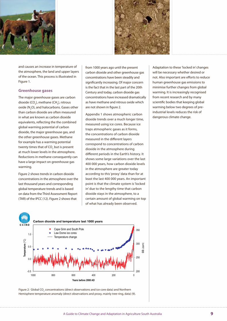
Figure 1: Details of Earth’s energy balance (source: Kiehl and Trenberth, 1997) . Numbers are in watts per square meter of Earth’s surface, and some may be uncertain by as much as 20% . The greenhouse effect is associated with the absorption and reradiation of energy by atmospheric greenhouse gases and particles, resulting in a downward flux of infrared radiation from the atmosphere to the surface (back radiation) and therefore in a higher surface temperature . Note that the total rate at which energy leaves Earth (107 W/m2 of reflected sunlight plus 235 W/m2 of infrared [long-wave] radiation) is equal to the 342 W/m2 of incident sunlight . Thus Earth is in approximate energy balance in this analysis (25) .
Reasons for uncertainty in climate change projections
In 2006, the Climate Impacts and Risk Group of the CSIRO prepared a report for the South Australian Government on climate change in SA and the Natural Resources Management (NRM) Regions (6) . In order to project climate change in South Australia, 23 global climate model (GCM) experiments, with the addition of two regional climate models, were assessed for their ability to simulate observed average (1961–1990) patterns of mean sea level pressure, temperature and rainfall in the South Australian region . Of these 13 performed satisfactorily . Temperature and rainfall projections were made using the results from those 13 models for South Australia .
Projections from the 13 models cannot be exact due to:
The uncertainty about the volume of greenhouse gases which will continue to be emitted into the atmosphere; this depends on the effectiveness of measures to reduce emissions and the trend in global population .
Uncertainty about the impact of increased greenhouse gas emissions at a regional scale .
Uncertainty in the climate science, in particular sensitivity of the climate system to increases in greenhouse gas levels .
What is clear to date are the measured trends in greenhouse emissions illustrated in many scientific papers and illustrated to the right .
What is the greenhouse effect?
Shortwave energy radiated by the sun enters the atmosphere surrounding the Earth and heats the Earth’s surface . The energy is re-radiated from the Earth’s surface back towards space in the form
of long wave radiation . As the energy passes back through the atmosphere, greenhouse gases (chiefly water vapour, carbon dioxide, methane, nitrous oxide and halocarbons in the troposphere) absorb part of the heat . The absorbed energy heats the lower layers of the atmosphere, and is re-radiated by the gases heating the land surface and upper layers of the ocean . This effect has been labelled ‘greenhouse’ because of the warming effect, but is in fact a different mechanism from greenhouses used in horticulture .
The Greenhouse effect in the atmosphere occurs naturally in response to levels of greenhouse gases which have remained relatively stable in the atmosphere until the start of the Industrial Era (~1750), when humans began burning large amounts of fossil fuels and clearing forest on a large scale . Burning fossil fuels ( coal,
oil etc) releases carbon dioxide into the atmosphere .
Trees are natural stores of carbon . Land clearing results in the decomposition of trees converting the carbon into carbon dioxide which is then released into the atmosphere .
The natural greenhouse effect is enhanced in the Earth’s atmosphere with increases in the concentration of greenhouse gases, chiefly from the carbon dioxide released from the processes mentioned above . Prior to 1750 carbon dioxide levels were ~280 parts per million . An increase of 30% has occurred since then to 380 parts per million at present . The rate of increase is ~1 .5 parts per million per year but this rate is increasing .
An increased concentration of greenhouse gases retains more of the heat which is usually radiated into space by the Earth
A Guide to Climate Change and Adaptation in Agriculture South Australia 9
Carbon dioxide and temperature last 1000 years
200
250
300
350
02004006008001000
Years before 2000 AD
-0.5
0.0
0.5
1.0
Tem
per
atu
re(°
C)
Cape Grim and South Pole
Law Dome ice cores
Temperature change
CO
2(p
pm)
Figure 2: Global CO2 concentrations (direct observations and ice core data) and Northern Hemisphere temperature anomaly (direct observations and proxy, mainly tree-ring, data) (9) .
and causes an increase in temperature of the atmosphere, the land and upper layers of the ocean . This process is illustrated in Figure 1 .
Greenhouse gases
The major greenhouse gases are carbon dioxide (CO2), methane (CH4), nitrous oxide (N2O), and halocarbons . Gases other than carbon dioxide are often measured in what are known as carbon dioxide equivalents, reflecting the the combined global warming potential of carbon dioxide, the major greenhouse gas, and the other greenhouse gases . Methane for example has a warming potential twenty times that of CO2 but is present at much lower levels in the atmosphere . Reductions in methane consequently can have a large impact on greenhouse gas warming .
Figure 2 shows trends in carbon dioxide concentrations in the atmosphere over the last thousand years and corresponding global temperature trends and is based on data from the Third Assessment Report (TAR) of the IPCC (12) . Figure 2 shows that
from 1000 years ago until the present carbon dioxide and other greenhouse gas concentrations have been steadily and significantly increasing . Of major concern is the fact that in the last part of the 20th Century and today, carbon dioxide gas concentrations have increased dramatically as have methane and nitrous oxide which are not shown in figure 2 .
Appendix 1 shows atmospheric carbon dioxide trends over a much longer time, measured using ice cores . Because ice traps atmospheric gases as it forms, the concentrations of carbon dioxide measured in the different layers correspond to concentrations of carbon dioxide in the atmosphere during different periods in the Earth’s history . It shows some large variations over the last 400 000 years, how carbon dioxide levels in the atmosphere are greater today according to this ‘proxy’ data than for at least the last 400 000 years . An important point is that the climate system is ‘locked in’ due to the lengthy time that carbon dioxide stays in the atmosphere, to a certain amount of global warming on top of what has already been observed .
Adaptation to these ’locked in’ changes will be necessary whether desired or not . Also important are efforts to reduce human greenhouse gas emissions to minimise further changes from global warming . It is increasingly recognised from recent research and by many scientific bodies that keeping global warming below two degrees of pre-industrial levels reduces the risk of dangerous climate change .
1
A Guide to Climate Change and Adaptation in Agriculture South Australia10
Figure 3: The bar graph shows estimated greenhouse gas emissions for all Australian sectors . Pie-chart shows the components of the 18% of emissions for which Australian agriculture was responsible in 2003 (from ‘Agriculture Industry Partnerships – Climate Change Action for Multiple Benefits’, Australian Greenhouse Office, 2006) .
Agricultural greenhouse gas emissions
The National Greenhouse Gas Inventory reports that agriculture in Australia produced an estimated 93 .1 million tonnes of carbon dioxide equivalent emissions (Mt CO2-e1) in terms of global warming potential or 16 .5% of net national emissions in 2002 (Figure 3) .
The agriculture sector is the dominant national source of both methane and nitrous oxide accounting for 71 .9 Mt CO2-e (60 .1%) of the net national emissions of methane and 21 .3 Mt CO2-e (86 .1%) of the net national emissions of nitrous oxide .
In 2002, agriculture contributed at least 20% of South Australia’s greenhouse gas emissions, or more than 6 .2 million tonnes of carbon dioxide equivalents (CO2-e) per year . However agriculture has potential to play a significant role in managing emissions to reduce the rate of
climate change . This is because the way soils, crops and pastures are managed can determine whether they are a source or a sink for greenhouse emissions .
The figures above include agricultural emissions from:
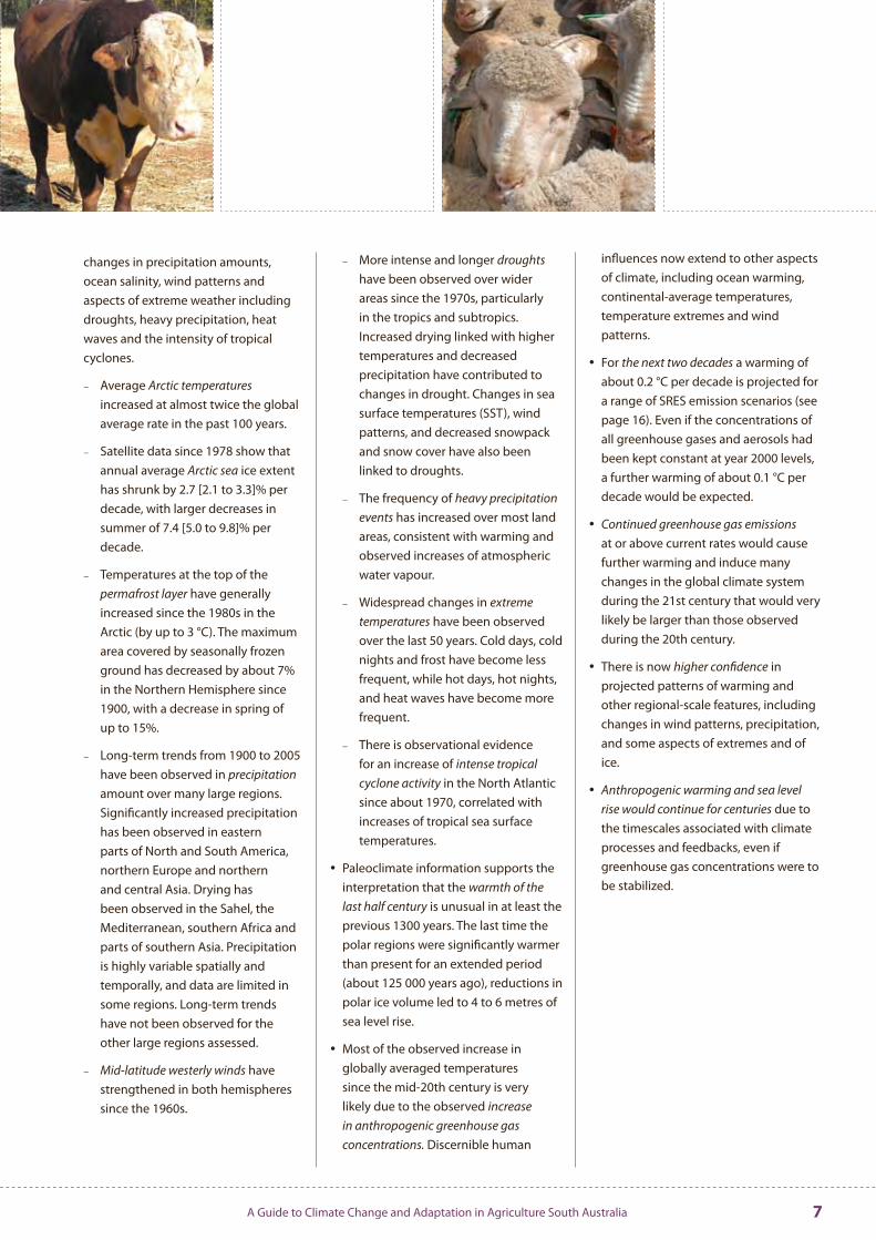
Livestock enteric fermentation (60% of total South Australian agricultural CO2-e emissions) — methane emissions resulting from the digestive processes of livestock (98% is emitted by cattle and sheep) .
1 A volume of greenhouse gas emissions with the global warmin potential equivalent to that of 93 .1 million tonnes of carbon dioxide .
0
50
100
150
200
250
300 49%
15%
5% 6%
18%
6% 2%
Stationaryenergy
Transport Fugitiveemissons
Industrialprocesses
Agriculture Land use changeand forestry
Waste
Contribution to Australia’s total greenhouse gas emissions by sector, 2003
Manure Management = 3.3 Mt
Rice cultivation = 0.4 Mt
Agricultural soils= 18.7 Mt
Enteric fermentation(methane from livestock)
= 62.7 Mt
Stubble burning = 0.3 Mt
Savanna burning= 11.8 Mt
Greenhouse gas emissions from Australian agriculture, 2003
Mt = Million tonnes of greenhousegas emissions
A Guide to Climate Change and Adaptation in Agriculture South Australia 11
Agricultural soils management (34% of total South Australian agricultural CO2-e emissions) — nitrous oxide emissions associated with soil disturbance, fertiliser losses and manure applications .
Manure management (5% of total South Australian agricultural CO2-e emissions) — both methane and nitrous oxide emissions generated by anaerobic decomposition of animal wastes .
However, the figures for agricultural emissions do not include emissions associated with agricultural transport (e .g . use of tractors and other vehicles on farms, transport of produce) or stationary energy use (e .g . electricity use by farms, for pumps, heating, and refrigeration) .
Carbon sequestration
Plants take up and store carbon by incorporating that carbon into their structure . These plant processes are collectively known as carbon bio-sequestration, which removes about 3 .2 million tonnes of CO2-e per year Australia-wide .
Greenhouse gas emissions from agriculture increased by 2 .2% (2 .0 Mt) between 1990 and 2004, but decreased by 1 .7% (1 .6 Mt) from 2003 to 2004 . Decreases in agricultural emissions can occur as a result of change in land use (e .g . less land being used for agricultural activities, particularly those causing emissions) or reduced stock numbers, for example .
Trends in agricultural emissions and sinks
Enteric fermentation emissions — There was only a limited change in enteric emissions over the five years to 2005 . During this time there was an increase in cattle numbers and a decrease in sheep . Reduced stock numbers because of the 2006–2007 drought will probably result in reduced methane emissions, at least in the short term .
Soil emissions — Emissions resulting from soil management (primarily nitrous oxide) have increased by approximately 20% from 1990 base emissions levels . This may be attributed to an increase in cropping or use of fertilisers . Of concern is recent research from the UK suggesting that as soil warms due to global warming, soils that were carbon dioxide sinks can become sources of carbon dioxide emissions .
Manure management — Emissions have increased by 40–43% from 1990 base levels .
A Guide to Climate Change and Adaptation in Agriculture South Australia12
2Chapter TWO
Climate change trends
Information on greenhouse gas emissions is based on scientific observations by thousands of scientists around the world for the International Panel on Climate Change (IPCC) .
The IPCC now considers that greenhouse gas emissions are very likely to be contributing to the trends in climate we have been experiencing . How much is part of natural variability and how much is attributable to greenhouse emissions and human activity is discussed below .
Analysis of these trends helps us to identify the risks to which we are exposed and the frequency of occurrence of adverse conditions . These frequencies can be expressed as a probability, such as one year in two, or 50% of the time . Analysis of the trends will also allow us to predict the probability of adverse conditions resulting from climate change .
Climate change trends
The basic parameters of weather — temperature, precipitation and wind are already changing:
Higher maximum, minimum and average temperatures are being recorded in most (but not all) areas . Restricted, local geographic variations may cause small localised reductions in temperatures .
Changes in rainfall patterns, encompassing timing and distribution of rainfall, have already been observed . For example, in the southwest of Western Australia stream flows fell to
75% of historic levels after 1975 and to about 60% of those levels after 1995 (19) .
As atmospheric temperatures rise inconsistently and heat is redistributed through greater movement of the air, which is, wind . Even a small difference in sea surface temperature is believed to be responsible for more destructive cyclone and hurricane activity .
Temperature trends
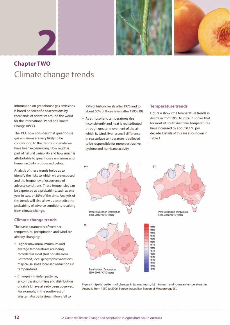
Figure 4 shows the temperature trends in Australia from 1950 to 2006 . It shows that for most of South Australia, temperatures have increased by about 0 .1 °C per decade . Details of this are also shown in Table 1 .
Figure 4: Spatial patterns of changes in (a) maximum, (b) minimum and (c) mean temperatures in Australia from 1950 to 2006 . Source: Australian Bureau of Meteorology (6) .
(a) (b)
(c)
Trend in Mean Temperature1950–2006 (°C/10 years)
Trend in Minimum Temperature1950–2006 (°C/10 years)
Trend in Maximum Temperature1950–2006 (°C/10 years)
A Guide to Climate Change and Adaptation in Agriculture South Australia 13
Table 1: Observed temperature trend increases for Australia and South Australia (6) .
Time period Average Minimum Maximum
Australia 1910 to 2005 +0 .89 °C
(+0 .09 °C per decade)
+1 .14 °C
(+0 .12 °C per decade)
+0 .65 °C
(+0 .07 °C per decade)
1950 to 2005 +0 .95 °C
(+0 .17 °C per decade)
+1 .04 °C
(+0 .18 °C per decade)
+0 .86 °C
(+0 .15 °C per decade)
South Australia
1910 to 2005 +0 .96 °C
(+0 .1 °C per decade)
+1 .13 °C
(+0 .12 °C per decade)
+0 .79 °C
(+0 .08 °C per decade)
1950 to 2005 +1 .2 °C
(+0 .21 °C per decade)
+1 .01 °C
(+0 .18 °C per decade)
+1 .1 °C
(+0 .2 °C per decade)
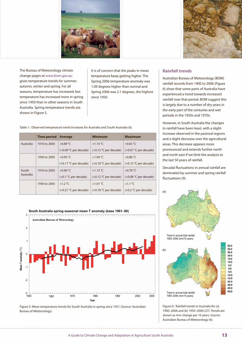
The Bureau of Meteorology climate change pages at www .bom .gov .au gives temperature trends for summer, autumn, winter and spring . For all seasons, temperature has increased, but temperature has increased more in spring since 1950 than in other seasons in South Australia . Spring temperature trends are shown in Figure 5 .
It is of concern that the peaks in mean temperature keep getting higher . The Spring 2006 temperature anomaly was 1 .09 degrees higher than normal and Spring 2006 was 2 .1 degrees, the highest since 1950 .
Rainfall trends
Australian Bureau of Meteorology (BOM) rainfall records from 1900 to 2006 (Figure 6) show that some parts of Australia have experienced a trend towards increased rainfall over that period . BOM suggest this is largely due to a number of dry years in the early part of the centuries and wet periods in the 1950s and 1970s .
However, in South Australia the changes in rainfall have been least, with a slight increase observed in the pastoral regions and a slight decrease over the agricultural areas . This decrease appears more pronounced and extends further north and north east if we limit the analysis to the last 50 years of rainfall .
Decadal fluctuations in annual rainfall are dominated by summer and spring rainfall fluctuations (9) .
Figure 6: Rainfall trends in Australia for (a) 1900–2006 and (b) 1950–2006 (27) . Trends are shown as mm change per 10 years . Source: Australian Bureau of Meteorology (6) .
Figure 5: Mean temperature trends for South Australia in spring since 1951 (Source: Australian Bureau of Meteorology) .
(a)
(b)
Trend in annual total rainfall1950–2006 (mm/10 years)
Trend in annual total rainfall1900–2006 (mm/10 years)
A Guide to Climate Change and Adaptation in Agriculture South Australia14
2Figure 7 shows the rainfall trends for summer, autumn, winter and spring in South Australia between 1950 and 2006 . The autumn rainfall has decreased for all arable areas in South Australia and winter rainfall has decreased in the western half of South Australia . Spring rainfall has increased slightly for most of the state, between 1950 and 2006, except for the south east corner . However it is not clear how much of these changes are due to natural variability and how much is due to greenhouse induced climate change .
General projections resulting from climate change are also for rainfall to occur in less frequent and more intense events resulting in increased runoff, erosion and flooding risks .
Figure 7: Rainfall trends in South Australia for 1950–2006 for summer, autumn, winter and spring (27) . Trends are shown as mm change per 10 years . Source: Australian Bureau of Meteorology .
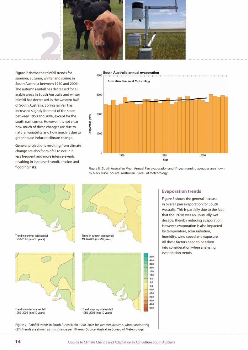
Figure 8: South Australian Mean Annual Pan evaporation and 11-year running averages are shown by black curve . Source: Australian Bureau of Meteorology .
Evaporation trends
Figure 8 shows the general increase in overall pan evaporation for South Australia . This is partially due to the fact that the 1970s was an unusually wet decade, thereby reducing evaporation . However, evaporation is also impacted by temperature, solar radiation, humidity, wind speed and exposure . All these factors need to be taken into consideration when analysing evaporation trends .
Trend in summer total rainfall1950–2006 (mm/10 years)
Trend in autumn total rainfall1950–2006 (mm/10 years)
Trend in winter total rainfall1950–2006 (mm/10 years)
Trend in spring total rainfall1950–2006 (mm/10 years)
A Guide to Climate Change and Adaptation in Agriculture South Australia 15
3Chapter THREE
Climate change projections
Using models to project changes in rainfall, temperature, water availability and extremes in climatic variables enables us to identify the threats or risks imposed on agriculture . Our understanding of climate change, its impacts and the actions we can take to deal with it are changing and evolving rapidly . Global Climate Models (GCMs), the models from which projections are made, are improving and growing steadily more reliable . Projections of impacts and consequences are becoming more specific and options for action are becoming clearer .
Climate change projectionsCSIRO Marine & Atmospheric Research released an updated report in 2006 on climate change (projections) under enhanced greenhouse conditions in South Australia (6), commissioned by the South Australian Government . The researchers selected 13 GCMs to produce projections of rainfall and temperature to 2030 and 2070 . These 13 GCMs were selected from 23 as being those that best simulate observed average patterns of mean sea level pressure, temperature and rainfall (1961–1990) in the SA region .
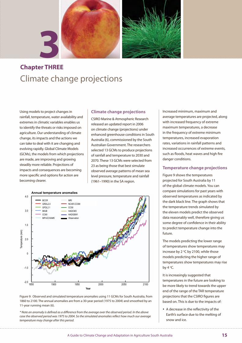
Figure 9: Observed and simulated temperature anomalies using 11 GCMs for South Australia, from 1860 to 2100 . The annual anomalies are from a 30-year period (1975 to 2004) and smoothed by an 11-year running mean (6) .
Increased minimum, maximum and average temperatures are projected, along with increased frequency of extreme maximum temperatures, a decrease in the frequency of extreme minimum temperatures, increased evaporation rates, variations in rainfall patterns and increased occurrences of extreme events, such as floods, heat waves and high fire danger conditions .
Temperature change projections
Figure 9 shows the temperatures projected for South Australia by 11 of the global climate models . You can compare simulations for past years with observed temperatures as indicated by the dark black line . The graph shows that the temperature trends simulated by the eleven models predict the observed data reasonably well, therefore giving us some degree of confidence in their ability to predict temperature change into the future .
The models predicting the lower range of temperatures show temperatures may increase by 2 oC by 2100, while those models predicting the higher range of temperatures show temperatures may rise by 4 oC .
It is increasingly suggested that temperatures in the future are looking to be more likely to trend towards the upper end of the range of the TAR temperature projections that the CSIRO figures are based on . This is due to the impacts of:
A decrease in the reflectivity of the Earth’s surface due to the melting of snow and ice .
* Note an anomaly is defined as a difference from the average over the observed period. In the above case the observed period was 1975 to 2004. So the simulated anomalies reflect how much our average temperature may change after this period.
T emp
eratu
re(m
m)
4.0
3.0
2.0
-1.0
-2.01850 1950 2000
Year
Annual temperature anomalies
1900 2050 2100
BCCRGRDL2.0GFDL2.1MIUBCC60MPI-ECHAM5
MRINCAR-CCSMCC50HADCM3HADGEM1Observation
1.0
0
A Guide to Climate Change and Adaptation in Agriculture South Australia16
Annual Summer Autumn Winter Spring
SRES 2030
0 1 2 3 4 5 6 7
Temperature Change (°C)
WRE450 2030WRE550 2030
SRES 550 ppm 450 ppm
SRES 2070 WRE450 2070WRE550 2070
SRES 550 ppm 450 ppm
2030
2070
0 1 2 3 4 5 6 7
Temperature Change (°C)
0 1 2 3 4 5 6 7
Temperature Change (°C)
0 1 2 3 4 5 6 7
Temperature Change (°C)
0 1 2 3 4 5 6 7
Temperature Change (°C)
0 1 2 3 4 5 6 7
Temperature Change (°C)
3The release of extra carbon dioxide and methane from the terrestrial biosphere .
A projected decrease in the concentration of aerosols, which have a cooling effect in the atmosphere (6) .
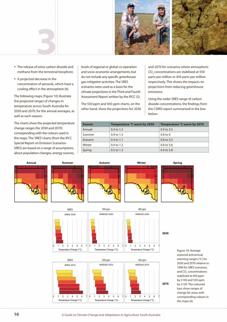
The following maps (Figure 10) illustrate the projected ranges of changes in temperature across South Australia for 2030 and 2070, for the annual averages, as well as each season .
The charts show the projected temperature change ranges (for 2030 and 2070) corresponding with the colours used in the maps . The ‘SRES’ charts (from the IPCC Special Report on Emission Scenarios - SRES) are based on a range of assumptions about population changes, energy sources,
Season Temperature °C warm by 2030 Temperature °C warm by 2070
Annual 0 .4 to 1 .2 0 .9 to 3 .5
Summer 0 .4 to 1 .3 0 .8 to 4
Autumn 0 .4 to 1 .1 0 .8 to 3 .5
Winter 0 .4 to 1 .2 0 .8 to 3 .6
Spring 0 .5 to 1 .3 0 .9 to 3 .8
levels of regional or global co-operation and socio-economic arrangements, but do not include any specific greenhouse gas mitigation activities . The SRES scenarios were used as a basis for the climate projections in the Third and Fourth Assessment Report written by the IPCC (5) .
The 550 ppm and 450 ppm charts, on the other hand, show the projections for 2030
and 2070 for scenarios where atmospheric CO2 concentrations are stabilised at 550 parts per million or 450 parts per million respectively . This shows the impacts on projections from reducing greenhouse emissions .
Using the wider SRES range of carbon dioxide concentrations, the findings from the CSIRO report summarised in the box below:
Figure 10: Average seasonal and annual warming ranges (oC) for 2030 and 2070 relative to 1990 for SRES scenarios, and CO2 concentrations stabilised at 450 ppm by 2100 and 550 ppm by 2150 . The coloured bars show ranges of change for areas with corresponding colours in the maps (6) .
A Guide to Climate Change and Adaptation in Agriculture South Australia 17
The images show that temperatures inland are likely to increase more than in coastal regions . The further inland you go, the warmer it may become . If greenhouse emissions can be restricted, and increases in atmospheric concentrations mitigated, the temperature changes projected at the other end of the scale are reduced . However the lower end will not change .
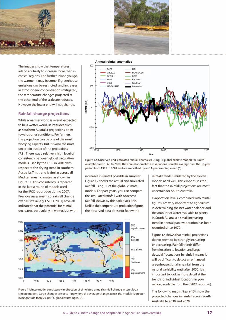
Rainfall change projectionsWhile a warmer world is overall expected to be a wetter world, in latitudes such as southern Australia projections point towards drier conditions . For farmers, this projection can be one of the most worrying aspects, but it is also the most uncertain aspect of the projections (7,8) . There was a relatively high level of consistency between global circulation models used by the IPCC in 2001 with respect to the drying trend in southern Australia . This trend is similar across all Mediterranean climates, as shown in Figure 11 . This consistency is repeated in the latest round of models used for the IPCC report due during 2007 . Previous assessments of rainfall change over Australia (e .g . CSIRO, 2001) have all indicated that the potential for rainfall decreases, particularly in winter, but with
Figure 11: Inter-model consistency in direction of simulated annual rainfall change in ten global climate models . Large changes are occurring where the average change across the models is greater in magnitude than 5% per OC global warming (5, 9) .
Figure 12: Observed and simulated rainfall anomalies using 11 global climate models for South Australia, from 1860 to 2100 . The annual anomalies are variations from the average over the 30-year period from 1975 to 2004 and are smoothed by an 11-year running mean (6) .
increases in rainfall possible in summer . Figure 12 shows the actual and simulated rainfall using 11 of the global climate models . For past years, you can compare the simulated rainfall with observed rainfall shown by the dark black line . Unlike the temperature projection figure, the observed data does not follow the
rainfall trends simulated by the eleven models at all well . This emphasises the fact that the rainfall projections are most uncertain for South Australia .
Evaporation levels, combined with rainfall figures, are very important to agriculture in determining the net water balance and the amount of water available to plants . In South Australia a small increasing trend in annual pan evaporation has been recorded since 1970 .
Figure 12 shows that rainfall projections do not seem to be strongly increasing or decreasing . Rainfall trends differ from location to location and large decadal fluctuations in rainfall means it will be difficult to detect an enhanced greenhouse signal in rainfall from the natural variability until after 2050 . It is important to look in more detail at the trends for individual locations in your region, available from the CSIRO report (6) .
The following maps (Figure 13) show the projected changes in rainfall across South Australia to 2030 and 2070 .
200
100
0
-100
-2001850 1950 2000
Year
Rain
fall (
mm)
Annual rainfall anomalies
1900 2050 2100
BCCRGRDL2.0GFDL2.1MIUBCC60MPI-ECHAM5
MRINCAR-CCSMCC50HADCM3HADGEM1Observation
A Guide to Climate Change and Adaptation in Agriculture South Australia18
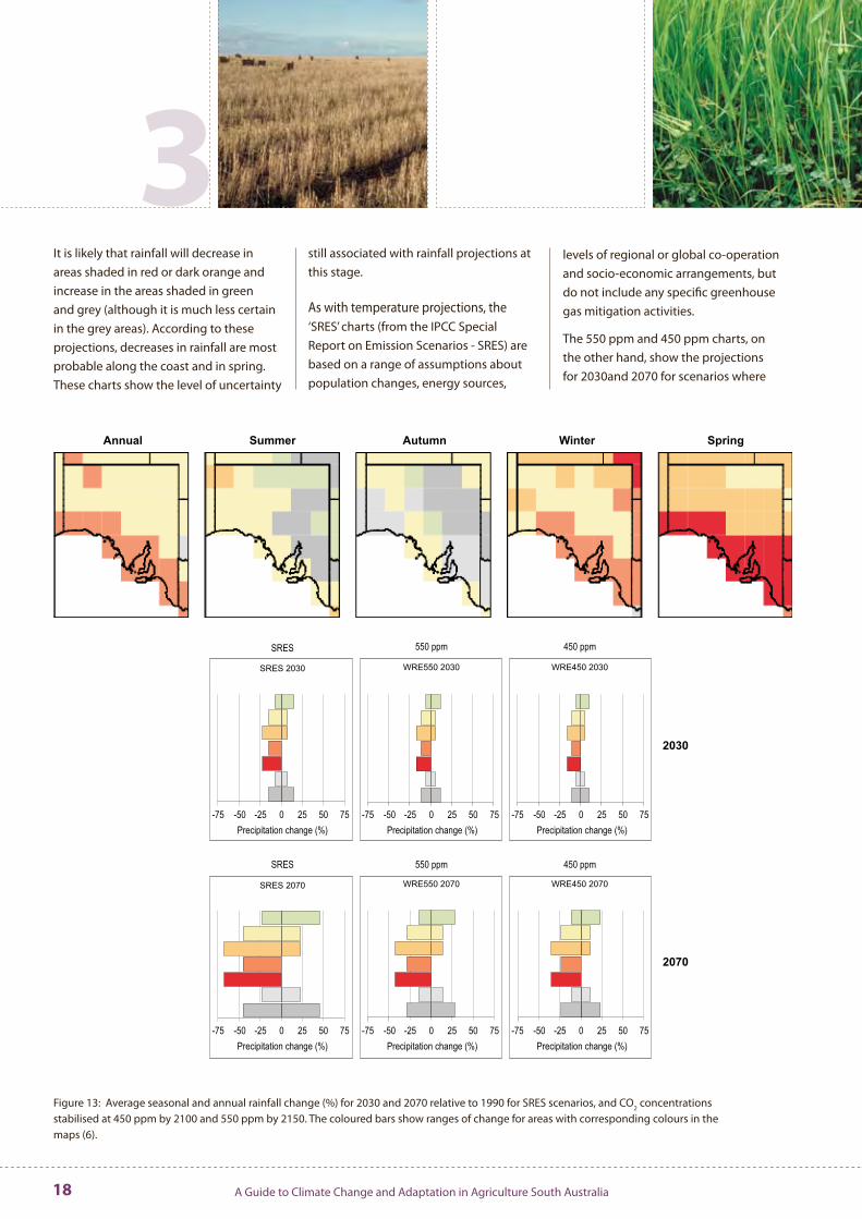
It is likely that rainfall will decrease in areas shaded in red or dark orange and increase in the areas shaded in green and grey (although it is much less certain in the grey areas) . According to these projections, decreases in rainfall are most probable along the coast and in spring . These charts show the level of uncertainty
3
Figure 13: Average seasonal and annual rainfall change (%) for 2030 and 2070 relative to 1990 for SRES scenarios, and CO2 concentrations stabilised at 450 ppm by 2100 and 550 ppm by 2150 . The coloured bars show ranges of change for areas with corresponding colours in the maps (6) .
still associated with rainfall projections at this stage .
As with temperature projections, the ‘SRES’ charts (from the IPCC Special Report on Emission Scenarios - SRES) are based on a range of assumptions about population changes, energy sources,
levels of regional or global co-operation and socio-economic arrangements, but do not include any specific greenhouse gas mitigation activities .
The 550 ppm and 450 ppm charts, on the other hand, show the projections for 2030and 2070 for scenarios where
-75 -50 -25 0 25 50 75
Precipitation change (%)
-75 -50 -25 0 25 50 75
Precipitation change (%)
-75 -50 -25 0 25 50 75
Precipitation change (%)
-75 -50 -25 0 25 50 75
Precipitation change (%)
-75 -50 -25 0 25 50 75
Precipitation change (%)
-75 -50 -25 0 25 50 75
Precipitation change (%)
Annual Summer Autumn Winter Spring
SRES 2030 WRE450 2030WRE550 2030
SRES 550 ppm 450 ppm
SRES 2070 WRE450 2070WRE550 2070
SRES 550 ppm 450 ppm
2030
2070
A Guide to Climate Change and Adaptation in Agriculture South Australia 19
atmospheric CO2 concentrations are stabilised at 550 parts per million or 450 parts per million respectively . This shows the impacts on projections from reducing greenhouse emissions .
Water balance and evaporation projections
One of the most important interactions between rainfall and temperature is the moisture balance . Generally as temperature rises evaporation increases . The small rise in average temperatures in Australia has generally not been accompanied by very slight rise in evaporation . There are a number of possible reasons for this with changes in wind and changes in instruments for recording evaporation being considered the most likely (20, 23) .
It is expected that further rises in temperature from global warming will be associated with increased evaporation and decreased soil moisture . This would exacerbate the consequences of a drying trend .
Extreme events projections
A range of extreme events is expected to occur under conditions of climate change and may already be evident, including unusually violent storms, high winds, extreme storm surges, more intense heatwaves, bushfires, drought and
flooding .
The frequency of extreme maximum temperatures will increase while the frequency of extreme minimum temperatures will decrease .
The frequency of hot spells above 35 °C and 40 °C are projected to increase across most of South Australia with the largest increases in the north .
Despite decreases of up to 30% in average rainfall over parts of South Australia in some seasons, the incidence
of heavy rainfall is projected to increase by 0 to 10% . The specific weather patterns associated with heavy summer rainfall in the north of the state are projected to increase both in terms of frequency of events and magnitude of rainfall, with a projected 20% increase in flood frequency in northern South Australia .
All climate models show an increase in the frequency of droughts in Australia towards the end of this century (9) .
Extreme events at the coast
Storm surges of at least half a metre in height occur year round along the South Australian coast with the greatest frequency of events occurring during the winter and spring months . They are caused by the westerlies or south-westerlies following the passage of cold fronts and their associated mid-latitude low pressure systems further to the south .
The frequency of winter time low pressure systems (lows) is projected to decrease by about 20% in the vicinity of South Australia under enhanced greenhouse conditions . Central pressures of the most extreme lows in model projections were lower by about 2 hPa on average, indicating slightly more intense lows under enhanced greenhouse conditions . Accumulated rainfall accompanying the lows in the South Australian region decreased by between 10 and 20% under enhanced greenhouse conditions owing to fewer low systems occurring . The amount of rainfall per low, however, tended to increase by up to 10% over the Bight and coastal regions in the western half of the state . The frequency of mid-latitude lows in spring increased by 2% while the most extreme lows deepened by about 1 hPa (6) .
Extreme wind speeds are projected to decrease across much of South Australia and the Bight in winter and summer . Increases in extreme wind speed occurred in model projections over the north of the state in autumn and while spring decreases occurred in the south of the State and over the Bight .
Examination of wind direction changes, particularly in westerlies, south-westerlies and southerlies, that can be responsible for storm surge occurrence in South Australia, revealed only minor changes in winter in South Australia with south-westerly coastal regions tending towards decreases in frequency . However, there were relatively larger increases in frequency of westerlies, south-westerlies and southerlies in eastern coastal regions in spring . Patterns of change were qualitatively similar in autumn but weaker than in spring while in summer, increases occurred only in the frequency of southerlies (9) .
In addition, the sea level has been projected to rise by 9 to 88 centimetres by 2100 (9) . However, recent observations have shown that Arctic and Antarctic ice is being lost at a rate significantly greater than that which had been projected, which means there is a risk of considerable increase in sea level rise projections .
A Guide to Climate Change and Adaptation in Agriculture South Australia20
4Chapter FOUR
Climate change impacts on agriculture
Likely impacts of climate change on agriculture
Changes to carbon dioxide, temperature, rainfall and wind conditions are expected to cause a range of local impacts as
described below .
The enterprises and regions most at risk will be:
Those already stressed – economically or biophysically (e .g . as a result of land degradation, soil salinity or loss of biodiversity) .
Those at the edge of their climatic range or tolerance .
Those where large and long-lived investments are being made — for example, dedicated irrigation systems, slow growing cultivars, and processing facilities .
Following are some likely impacts on agriculture .
Temperature impacts
Changes to crop yields and pasture growth, depending on the optimum temperature ranges for growth of each species or variety .
Reduced protein content for some grain crops, as a result of heatwaves .
Increased heat stress in livestock, resulting in reduced milk production, reduced meat production and quality, and increased mortality .
Increased frequency, speed and intensity of wildfires (more lightning
strikes and longer dry spells are likely to contribute to increased frequency of fires) .
Cool climate growing areas become unproductive for some traditional crops, such as cherries and cool climate wine grapes .
Warmer, moister conditions can result in the entry or proliferation of some weeds, pests and diseases (especially fungal infections) .
New crop or stock opportunities in areas previously considered too cool (e .g . warm climate fruits) .
Extended or changed (e .g . earlier) growing seasons, possibly leading to opportunities to enter markets by supplying produce earlier than do current suppliers .
Reduced vernalisation2 of fruit crops, due to increased minimum temperatures or less chilling .
Rainfall/water supply impacts
Reduced crop yields, when the negative impacts of reduced available moisture in the soil and atmosphere exceed the positive impacts of increased carbon dioxide concentration in the atmosphere .
Large regional differences in the impacts on crop yields — there is a high chance of decreases in productivity and value for wheat in Western Australia,
2 Vernalisation refers to a plant’s requirement for a period of cold temperature (or chilling) to initiate flowering .
but high chances of increases in Emerald (Qld) and Wagga Wagga (NSW) (10) .
Flow-on effects from changes in crop yields and crop prices for livestock industries, for which bought-in grains and other fodder is a major input cost .
Reduced pasture growth as a result of decreased winter and spring rainfall in southern Australia could significantly constrain animal production, under current farming systems (11) .
Greater demands on water resources, due to decreased supply and possibly increased demand .
Increased soil salinity and reduction in the area of productive agricultural land due to greater reliance on irrigation .
Increased erosion potential with heavy rainfall events .
Extreme events
Multiple impacts associated with more frequent, longer, and hotter droughts .
Crop/pasture and property damage associated with strong winds, flooding, hail and storms (and possibly loss of livestock and decreased livestock production) .
Coastal impacts
Increased salinity of water in estuaries due to sea level rise .
Possible reduction in the amount of water suitable for irrigation .
Possible reduction in area of land suitable for agriculture .
A Guide to Climate Change and Adaptation in Agriculture South Australia 21
Goyder’s line
Using likely scenarios of climate change derived from multiple climate models and emissions scenarios, Howden and Hayman examined the probability of shifts in Goyder’s line in South Australia, concluding there was a small probability of the line shifting north, but a larger probability of it shifting south, increasing pressure on marginal cropping zones (21) .
Ecosystem impacts
The productive ranges of native South Australian species of plants and animals are likely to change significantly, with a tendency towards shifts southerly and towards higher, cooler ground . Cleared land is likely to provide an obstacle to many species attempting to adopt these
changes .
Trade impacts
As climate change is a global phenomenon, costs and benefits will impact upon other regions, including Australia’s overseas agricultural competitors . In some situations that could threaten current South Australian advantages and marketing opportunities .
North America is expected to enjoy warmer conditions, leading to increased productivity and increased competition (supply) in international markets such as those for wheat and barley . Changes in temperature will alter animal husbandry requirements in Europe, allowing animals to be housed indoors for shorter periods, or not at all, substantially reducing production costs . Changes in pest and disease incidence, and severity of infestations, in crop and animal enterprises of Australia’s trading competitors are also likely to occur .
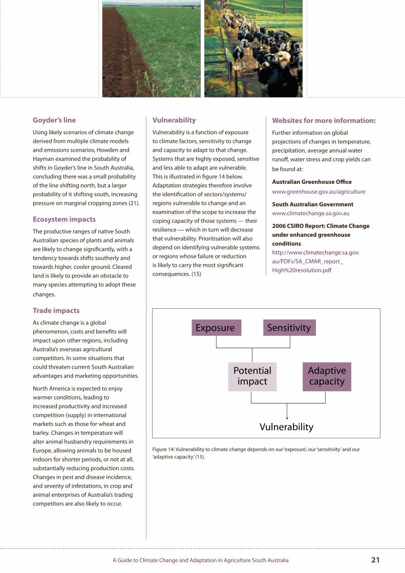
Vulnerability
Vulnerability is a function of exposure to climate factors, sensitivity to change and capacity to adapt to that change . Systems that are highly exposed, sensitive and less able to adapt are vulnerable . This is illustrated in figure 14 below . Adaptation strategies therefore involve the identification of sectors/systems/regions vulnerable to change and an examination of the scope to increase the coping capacity of those systems — their resilience — which in turn will decrease that vulnerability . Prioritisation will also depend on identifying vulnerable systems or regions whose failure or reduction is likely to carry the most significant consequences . (15)
Websites for more information:
Further information on global projections of changes in temperature, precipitation, average annual water runoff, water stress and crop yields can
be found at:
Australian Greenhouse Office
www .greenhouse .gov .au/agriculture
South Australian Government www .climatechange .sa .gov .au
2006 CSIRO Report: Climate Change under enhanced greenhouse conditions http://www .climatechange .sa .gov .au/PDFs/SA_CMAR_report_High%20resolution .pdf
Figure 14: Vulnerability to climate change depends on our ‘exposure’, our ‘sensitivity’ and our ‘adaptive capacity’ (15) .
Exposure Sensitivity
Potentialimpact
Adaptivecapacity
Vulnerability
A Guide to Climate Change and Adaptation in Agriculture South Australia22
5Chapter FIVE
Climate change mitigation and adaptation in agriculture
Having established the context of the risks to be managed and identified, analysed and evaluated, you are now in a position to deal with them .
The broad approach adopted by many
organisations, is to consider:
Reducing the risk by reducing greenhouse gas emissions .
Adapting your enterprise to the new conditions .
Applying innovative approaches that enable you to identify new opportunities in the projected changed environment .
Reducing greenhouse gas emissions at the farm level, while contributing to reduced atmospheric levels, also has the potential to generate on-farm savings through increased efficiency and more strategic use of resources .
This Guide also looks at adaptation and innovation, approaches that may be tailored to the individual farm, its business and its environment . On-farm adaptation and innovation also have the greatest chance of immediate benefit whatever the level of climate change .
Importantly, most of the measures you take to address climate change will be of benefit whatever the level to which your business is affected by climate change . You can consider it a win-win strategy; whatever the future, by careful assessment, planning and action, you will be better off!
Strategies for reducing greenhouse gas emissions
Carbon dioxide
Reduce consumption of fossil fuels (such as petrol, diesel, oil) and electricity . You may wish to undertake an ‘energy audit’ to identify the major uses of energy by your operation and key areas for improvement . Energy use can be reduced by changing practices, using new technology (i .e . energy efficient equipment) or using ‘cleaner’ sources of energy with lower emissions . Reduced energy use will mean reduced energy costs .
Implement reduced tillage systems (including conservation tillage, direct
drill and no till systems) to increase the retention of carbon and nitrogen in the soil .
Methane
Provide highly digestible stockfeed, such as good quality pasture or grain, to reduce methane production . This can be achieved by selecting suitable pasture species (or other fodder), and managing pasture with grazing rotations and adjusting the ration .
Increase production efficiency, select and breed animals with high conversion efficiencies (and lower emissions) or, alternatively, reduce animal numbers (particularly cattle) .
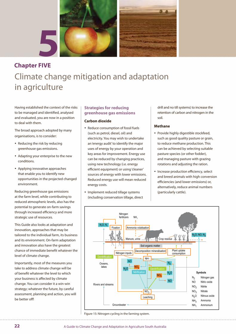
Figure 15: Nitrogen cycling in the farming system .
N O, NO, N2 2
Nitrogenfertilizers NH3
N O, N2 2
Fixation
Manure, urine
Nitrogen inputs
Ammonia volatisation
Soil organic matter
Decomposition mineralisation
Crop residue
Plant uptakeconsumption
NH1
Oceans,lakes
NO
N O2NO2
NitrificationDenitrification
NO2
N2
N O2
NO
NO3
Leaching
Rivers and streams
Groundwater
N2
NO
NO2
NO3
N O2
NH3
NH1
Nitrogen gas
Nitric oxide
Nitrite
Nitrate
Nitrous oxide
Ammonium
Ammonia
Symbols
Denitrification
A Guide to Climate Change and Adaptation in Agriculture South Australia 23
Use veterinary products, additives or digestive organisms (inoculation) to reduce emissions and increase conversion efficiency, where such use has been shown not to have significant negative impacts on animal health or welfare .
Use aerobic composting methods for organic waste . Anaerobic decomposition produces significantly more greenhouse gas than aerobic decomposition .
If you can convert more stockfeed to protein rather than methane, your production efficiency rises and you have the opportunity to become more profitable .
Nitrous oxide
Maximise precision of nitrogen applications, through careful timing and application methods .
Use appropriate fertiliser products and plant species, or combinations of plant species (e .g . appropriate rotations) .
Minimise losses of nitrogen by volatilisation (into ammonia or nitrous oxide) . This can be achieved, for example, by careful nutrient budgeting and good effluent management systems .
If you can ensure that the nitrogenous fertilisers that you apply are converted to the grain and plants you produce, then you not only reduce nitrous oxide emissions to the atmosphere but you also have the opportunity to reduce fertiliser applications and associated costs .
See figure 15 showing nitrogen cycling in the farming system .
Carbon sequestration
Grow forests or alternative woody crops to increase plant uptake of carbon dioxide (carbon sequestration, a form of bio-sequestration) . If an emissions trading scheme is established, opportunities may arise for selling the carbon sequestered to companies that generate electricity from coal, for example .
Increase soil carbon sequestration — through reduced till systems, cover crops or ‘green manure’ crops, appropriate crop rotations, perennial vegetation or pasture species, use of bio-solids for soil health and as a source of nutrients, and precision farming .
Resource use
Energy from fossil fuels is consumed (and therefore greenhouse gases are emitted) in the production of many products and services . Therefore prudent use, reuse, recycling and careful choice of products can reduce the volume of greenhouse gases emitted in the production of products or provision of services for your farming operation .
Adaptation in agriculture
The rate of climate change and the frequency and magnitude of extreme weather events will determine the impacts on South Australian agriculture in the future .
The key features of climate change that make agriculture vulnerable are related to variability and extremes, not simply changed average conditions . Agricultural communities are reasonably adaptable to gradual changes in average conditions . However, losses from climatic variations and extremes can be substantial and, in some sectors, are increasing (12) .
The ability to adapt and cope with impacts due to climate change depends on wealth, scientific and technical knowledge, information, skills, infrastructure, institutional arrangements and equity . Development decisions, activities and programs play important roles in modifying the adaptive capacity of communities and regions (12) .
Adaptive capacity
Most adaptive management is associated with developing the resilience of systems, thereby reducing the sensitivity and increasing the adaptive capacity of management systems . Failure to prioritise risks to be addressed appropriately (e .g . using inappropriate discounting) can
result in poor outcomes such as:
Under-adaptation — when climate change factors are given insufficient weight in decision-making .
Over-adaptation — when climate change factors are given too much weight .
Mal-adaptation — when decisions are taken that make an activity or region more vulnerable to climate change (13) .
Levels of treatmentGuidelines for assessing the degree of response to risk associated with climate change have been summarised by the United Nations Environment Programme . Some of these strategies are applicable to government action but many may be applied at the property level .
Bear the loss: In theory, bearing the loss occurs when those affected have no capacity to respond or where the costs of adaptive measures are considered to be high in relation to the risk or expected damage .
Share the loss: This may occur though reconstruction or rehabilitation paid for from public funds or private insurance .
A Guide to Climate Change and Adaptation in Agriculture South Australia24
Modify the threat: It is possible to put control measures in place for some risks, such as flood . For example, by putting better stormwater management systems or infrastructure in place .
Prevent or avoid effects: Most of these are discussed below . Examples include changes in crop variety, irrigation practices and pest and disease control .
Change use: Where the threat of climate change makes the continuation of an economic activity impossible or extremely risky, consideration can be given to changing the activity or land use . For example, cropping land may be returned to pasture or other uses may be found .
Adjust location: A more extreme response is to change the location of business activities . (This may be a feasible approach, but an unlikely option for most farmers e .g . moving from a low rainfall to high rainfall region) .
Research: The process of adaptation can also be advanced by research on new technologies and new methods of
adaptation .
Educate, inform and encourage behavioural change: Another type of adaptation is behavioural change through education and public information campaigns .
Priority scoring of climate risks
There are several methods for prioritising risks . One method developed by the Allen Consulting Group (15), is illustrated in table 2 . The example shows the impact of warmer conditions on winter wheat and chooses the risk projection to be 2 oC warmer in October . The table could be extended to add other risk projections and their priority for treatment . Table 2 suggests a 2 oC on average warming in
5
October means that adaptation measures to this risk are a high priority for sowing winter wheat .
Short term adaptive measures
Cropping and pasture
Here are some suggestions on how to adapt to climate change in the short term, taking into account potential climate variability and extremes, for cropping and grazing . It is suggested that each individual farmer adapt his own list or brain storm this in workshops .
Minimise high input costs on high-risk areas e .g . coastal flats .
Select crop and pasture species best suited to a variable climate .
Select a range of sowing times for your crops or pastures and plan for earlier or later harvests and rotations, based on seasonal outlooks .
For crops that mature in summer, it may be possible to select varities that mature earlier to avoid peak summer temperatures .
Maximise water use efficiency by:
using zero tillage
retaining crop residues
wider row spacing and lower seeding rates
−
−
−
monitoring soil moisture so timing of irrigation is optimal
Be vigilant for new or increased weed and disease and insect problems .
Reduce potential for soil erosion by:
retaining stubble
clay spreading or clay delving
reducing fallow times
reducing grazing pressure
reducing dry sowing in risky areas
establishing contour banks, where appropriate
Reduce potential for salinity by using deep-rooted plants in rotations .
Horticulture
Here are some suggestions on how to adapt to climate change in the short term, taking into account potential climate variability and extremes for horticulture:
Consider changing to varieties best suited to predicted conditions .
Monitor soil water conditions and improve the timeliness and quantity of irrigation .
Adjust systems to more drought tolerant, and heat stress tolerant species .
−
−
−
−
−
−
−
Table 2: Priority scoring of treatment of winter wheat .
Criteria Example 2 OC warmer in October
Exposure High
Sensitivity High
Adaptive capacity Medium
Adverse implications High
Potential to benefit Low
Overall priority High
A Guide to Climate Change and Adaptation in Agriculture South Australia 25
Adopt flexible, integrated pest management approaches as changing conditions may increasingly favour invasive species .
As irrigation demands increase in warmer weather, ensure irrigation systems optimise water use and reduce losses to the water table, to surface run-off, and evaporation .
Consider increased shade cover to reduce evaporation .
Consider other forms of enterprise, such as broad-acre cropping or intensive animal keeping, that may be more suited to the location .
Livestock
Here are some suggestions on how to adapt to climate change in the short term, taking into account potential climate variability and extremes, for livestock enterprises:
Adjust stocking rates and introduce diverse grazing and fodder options .
Select or breed animals more resilient to heat stress .
Reduce heat stress on stock by:
providing better shade and shelter
providing plenty of drinking water
Plant additional trees to provide protection against strong winds and storms .
Plan options for temporary stock feeding .
Plan additional watering options for expected longer dry spells .
Adopt fodder conservation and conserved fodder use strategies . Consider long term storage of fodder and the option of holding more fodder in reserve to address the higher likelihood of poor seasons .
−
−
Use feedlotting strategies, where appropriate, with careful planning .
Consider feed-lot systems to ease pressure on stressed pastures .
Trial drought tolerant pasture species .
Use seasonal outlooks to plan when animals will be less exposed at vulnerable stages like pregnancy or lambing or calving .
All farming enterprises
Here are further suggestions that all enterprises should consider when adapting to climate change and climate variability in the short term:
Have emergency response plans in place for fire, flood, hail and heavy rain .
Consider the water requirements of your operation and how the range of potential climatic conditions may affect both your operation’s water supply and water demands .
Improve water use efficiency .
Increase infiltration, reduce runoff, maintain water catchment areas, and increase drainage and runoff storage capacity .
Increase groundwater recharge, if appropriate .
Conserve existing waters and storages by reducing leakage, installing covers and increasing dam depth to reduce evaporation .
Consider treatment and recycling of wastewaters from other areas of the farm .
Consider possibilities of an on-site desalination plant .
Update bushfire preparedness .
Consider the financial risks and opportunities for your business including:
changes in input costs due to climatic changes (grain, fertiliser, insecticide, fuel, energy etc .)
changes in prices received (perhaps due to global supply and demand, which are also likely to be influenced by climatic changes)
Offset increased costs of managing for climate change by reducing energy use and related costs, for example, using more energy efficient equipment, installing alternative energy supplies (such as wind power) etc .
Use power and energy thoughtfully and conservatively to save energy, cost and to reduce greenhouse gas emissions .
Research developments in other regions, to explore ideas and different options trialled by others, and to remain aware of potential new market competition .
Maintain awareness of understanding of climate change and response strategies .
Longer term adaptive measures
Cropping
Consider a change in enterprise focus if temperature and evaporation are expected to significantly increase . In some areas, livestock may be a better option than cropping (16) .
Be aware of new varieties of crop and pasture species that may be more suited to hotter or drier conditions .
Grow deep rooted perennials which have the potential to improve water-use efficiencies of vegetation, lower water tables, minimise erosion, improve soil carbon inputs, provide shelter and shade and provide forage for stock (17) .
−
−
A Guide to Climate Change and Adaptation in Agriculture South Australia26
Agro-forestry offers direct benefits to landholders by diversifying production and providing longer term investment opportunities (including biosequestration and carbon trading) .
Mixed forestry-agriculture-pastoral systems have the potential to improve resilience of land use practices to
environmental change (16) .
All enterprises
Financial
Consider off-farm income for poor years .
Consider share farming to stabilise income .
Adopt precision agriculture technologies that will improve efficiencies of land, water and labour use, such as detailed monitoring of yields and fertiliser applications .
Water
Investigate methods of water conservation .
Monitor and modify water use to reduce use where practical .
Develop ground covers to improve water infiltration .
Science/knowledge
Increase your knowledge of climate change, how it will develop in your region, its impacts and current strategies for responding .
Use science along with experience to ensure appropriate responses .
Maintain good farm records to validate climate change on your property, the measures you take to manage the changes, and the value of the strategies you apply .
Review research on biological solutions for insect pests and diseases .
5Use information on projected long term climate change to develop long term plans .
Diversification
Look at opportunities that climate change may bring for carbon sequestration, new crops and water use efficiency .
Spread risks through multiple holdings in different climatic regions .
Look at practices undertaken in other, and more marginal, areas and consider their adoption in your region or enterprise .
Use indigenous species for the production of wood, fodder, biomass, oils, flowers and fruits for niche diversification .
Consider introducing crop and livestock species from areas that are currently warmer or drier than your own .
Seize opportunities for obtaining government or community funding that may be available to farmers for ecosystem services associated with revegetation (including carbon sequestration programs) and water management .
Policy
Be aware of existing policy on climate change and make sure that you or your industry are engaged in the development of future policy, for example, allocation of research funding for adaptation in agriculture .
Be aware of developments in greenhouse emissions (or carbon) trading and any implications (threats or opportunities) for your enterprise .
Be aware of, and engaged in the development of, policy affecting your water supply or its security .
For information on the history of government policy for greenhouse emissions and climate change go to Appendix 2 .
Further considerations
Agriculture has adaptive capacity . For example in 2005, despite a late break, low winter rainfall (typical trends as shown in figure 7), lower than normal growing season rainfall and a hotter than normal season across most of the South Australian cereal region, the yield was 7 .4 million tonnes per hectare, the highest recorded in South Australia for five years .
Flexibility in adapting to climate change will be the hallmark of minimising impact of climate change on agriculture and realizing opportunities that arise in production or marketing . Any limitations to flexibility such as from government, community and farmer conservatism, commercial or corporate influence, will be at agriculture’s expense . Market knowledge and involvement in strategy and action will be vital as climate change leads all producers and other industry members to reposition themselves in production and marketing .
Climate forecasting, as a risk management tool is always being improved and should be used to support management decisions in conjunction with seasonal conditions to date and projections .
Better tools and training for farmers and communities to improve their use of the available climate forecast data in their planning decisions will be important . Keep an eye open for new ideas and approaches to both production systems and climate change management .
Negative adaptive capacity
The capacity to adapt to climate change will be reduced by:
A Guide to Climate Change and Adaptation in Agriculture South Australia 27
Reliance on biological systems .
Reliance on long lived core assets .
Constraints imposed by current development patterns .
Inflexibility to change and innovation .
Positive adaptive capacity
Capacity to adapt to climate change will be improved by:
Ability to cope with current climate variability and similar ‘shocks’ (e .g . swings in international market prices .
Well established networks and mechanisms for generating and applying new knowledge .
Ability to manage and apply resources (property, stock, equipment, budgets etc .) with flexibility .
Climate change has been described as a worse threat to mankind than global terrorism . Whatever the severity of future climate impacts, natural resources and agricultural pursuits will not be immune to them . However, there are processes you can use to respond to climate change in a positive way, both to protect your interests and to identify new opportunities and new and more efficient ways of working .
You are not alone in this challenge . While strategies on your farm need to be tailored to your specific circumstances on your unique piece of land, there will be ideas generated by your neighbours and others that may assist you — and your ideas may assist them . It is valuable to work together to develop localised strategies and plans that can support the community, and your own operation, in your area . Impacts such as floods, for example, are rarely likely to affect your property in isolation; perhaps flood management measures and infrastructure
can be prepared collectively . And collectively, you are more likely to attract the attention of experts and advisers skilled in climate and farm management .
A Guide to Climate Change and Adaptation in Agriculture South Australia28
6Chapter SIX
Future considerations
This is not the first time farmers have needed to be resilient and work out solutions to problems . Farmers have always worked with a level of climate variability . In 50 to 100 years time, South Australian agriculture may be quite different; it is hoped that it will have adapted to new climatic conditions with a high level of success, with farmers making the most of new opportunities .
Monitoring
To confirm that you are on the right track, you will need to keep records of:
Conditions on your farm .
The management actions you apply .
The responses from the land and the production results you achieve that result from your actions .
The changes you make .
The investments you make, and how and where you make them .
The outcomes you experience, whether
or not they result from your actions .
Review
With your experience, captured in the records you have collected, you will be well positioned to review your strategy in managing climate change on your property . A review should be carried out regularly, say annually, perhaps more or less frequently, depending on the circumstances:
Were the results what you intended?
Did you invest time, effort or money in the right place at the right time?
Did you invest too much, or too little?
Was your strategy right for your business at this time?
What do you need to do differently, and in what time-frame?
Do you need more information or outside, specialist assistance?
Good luck!
A Guide to Climate Change and Adaptation in Agriculture South Australia 29
References and further reading
ReferencesStandards Australia (2004) . Australian Standard AS/NZS 4360:2004, Risk Management, Sydney, Australia .
Standards Australia (2004) . Risk Management Guidelines, Handbook, HB 436:2004, Sydney, Australia .
Australian Greenhouse Office (2006) . Climate Change Impacts & Risk Management, A Guide for Business and Government. Department of the Environment and Heritage, Canberra . Viewed 14 December 2006 <http://www .greenhouse .gov .au/impacts/publications/risk-management .html> .
Pittock B (2003) . Climate Change: An Australian Guide to the Science and Potential Impacts, Australian Greenhouse Office, Canberra . Viewed 12 Oct 2004 <http://www .greenhouse .gov .au/science/guide/pubs/science-guide .pdf> .
Intergovernmental Panel On Climate Change (2001) . Climate Change - The Scientific Basis . Contribution of Working Group I to the Third Assessment Report of the Intergovernmental Panel on Climate Change, Cambridge University Press, United Kingdom . Viewed 2 Sept 2004 <http://www .grida .no/climate/ipcc_tar/wg1/index .htm> .
Suppiah R, Preston B, Whetton PH, McInnes KL, Jones RN, Macadam I, Bathols J Kirono D (2006) . Climate Change under enhanced greenhouse conditions in South Australia, CSIRO Climate Impacts and Risk Group, CSIRO Marine and Atmospheric Research, a consultancy report for the South Australian Government . Viewed 8 Nov 2006 <http://www .climatechange .sa .gov .au/PDFs/SA_CMAR_report_High%20resolution .pdf> .
Hayman P (2006) . Climate change in the grains industry . Chapter in The Future
1 .
2 .
3 .
4 .
5 .
6 .
7 .
Environment of Grain Production . Rural Solutions, Jamestown, SA .
Hayman P (2006) . Linking climate change to SA grain farming systems . Presentation at Grains Research Development Corporation adviser updates, Adelaide Convention Centre .
McInnes KL, Suppiah R, Whetton PH, Hennessy KJ, Jones RN (2003) . Climate change in South Australia Report on: Assessment of climate change, impacts and possible adaptation strategies relevant to South Australia . CSIRO Atmospheric Research, <http://www .environment .sa .gov .au/sustainability/pdfs/csiro_report .pdf> .
Howden M, Jones R (2001) . Costs and benefits of CO2 increase and climate change on the Australian wheat industry, Australian Greenhouse Office . <www .greenhouse .gov .au/science/wheat/index .html> .
Clark A, Barratt D, Munro B, Sims J, Laughlin G, Poulter D (2006) . Climate change: Adaptation in agriculture, Australian Government, Bureau of Rural Sciences and Department of Agriculture, Fisheries and Forestry .
White (lead author) (2001) . Climate Change 2001: Impacts, adaptation and vulnerability . Technical Summary . A report for working Group II of the Intergovernmental Panel on Climate Change .
Willows RI, Connell RK (2003) . Climate Adaptation: Risk, Uncertainty and Decision making – UKCIP Technical Report .
Bardsley, D (2006) . There’s a change on the way - An initial integrated assessment of projected climate change impacts and adaptation options for Natural Resource Management in the Adelaide Mt Lofty Ranges Region, Department
8 .
9 .
10 .
11 .
12 .
13 .
14 .
of Water Land and Biodiversity report, Government of South Australia .
The Allen Consulting Group (2005) . Climate risk and vulnerability . Promoting an efficient adaptation response in Australia . Final Report to the Australian Greenhouse Office, Department of Environment and Heritage .
CSIRO Land and Water (2001) . The contribution of mid to low rainfall forestry and agroforestry to greenhouse and Natural Resource Management outcomes: Overview and analysis of opportunities . Australian Greenhouse Office and Murray Darling Basin Commission, Canberra .
Lefroy EC, Stirzaker RJ (1999) . Agroforestry for water management in the cropping zone of Southern Australia . Agroforestry Systems 45: 277-302 .
Productivity Commission (2005) . Trends in Australian Agriculture Research Paper, Australian Government, Canberra . <www .pc .gov .au/research/crp/agriculture/agriculture .pdf> .
IOCI (2002) . Climate variability and change in south west Western Australia . Indian Ocean Climate Initiative Panel . Department of Water and Catchment Protection, Perth WA .
Nichols N (2006) . Detecting and attributing Australian climate change: a review. School of Geography and Environmental Science, Monash University, Australia . Aust . Met . Mag . 55 (2006) 199-211 . In press .
Howden SM, and Hayman P (2005) . The distribution of cropping under climate change: Goyder’s line, Proc . Greenhouse 2005 conference, 14-17, December, Melbourne, Australia .
Flannery T (2005) . The weather makers . Text publishing, Melbourne .
15 .
16 .
17 .
18 .
19 .
20 .
21 .
22 .
A Guide to Climate Change and Adaptation in Agriculture South Australia30
Rayner DP (2006) . Wind run changes are the dominant factor affecting pan evaporation trends in Australia . Queensland Department of Natural Resources, Mines and Water, Indooroopilly .
Steffen W (2006) .Stronger evidence but new challenges: Climate Change Science 2001-2005, Australian Greenhouse Office, Department of the Environment and Heritage, Canberra .
Schneider S (2006) . Climate Science - The Greenhouse effect is scientifically well-established <www .stephenschneider .stanford .edu/Climate/Climate_Science/CliSciFrameset .html> .
Intergovernmental Panel on Climate Change (IPCC), 2 February 2007 . Climate Change 2007: The Physical Science Basis - Summary for Policy Makers, Contribution of Working Group 1 to the Fourth Assessment Report of the IPCC, IPCC, Geneva, Switzerland . Viewed February 2007 <http://www .ipcc .ch/SPM2feb07 .pdf> .
Australian Bureau of Meteorology, (2006) . The Greenhouse Effect and Climate Change . Viewed November 2006 <http://www .bom .gov .au/info/GreenhouseEffectAndClimateChange .pdf> .
Further readingAustralian Greenhouse Office (2006a) . Greenhouse and Agriculture, Department of the Environment and Heritage, Canberra . Viewed 8 Nov 2006 . <http://www .greenhouse .gov .au/agriculture/index .html> .
Australian Greenhouse Office (2006c) . Impacts and adaptation resources database, Department of the Environment and Heritage, Canberra . Viewed 8 Nov 2006 . <http://www .greenhouse .gov .au/impacts/database/index .html> .
Australian Greenhouse Office (2006) . National greenhouse gas inventory: analysis of recent tends and greenhouse indicators 1990 to 2004 . Department of the Environment and Heritage, Canberra .
23 .
24 .
25 .
26 .
27 .
<http://www .greenhouse .gov .au/inventory/2004/pubs/trends2004 .pdf> .
Australian Greenhouse Office (2002) . Pathways and policies for the development of a national emissions trading system for Australia – a response to specific issues raised by the Secretariat to the Council of Australian Governments Energy Market Review, Department of the Environment and Heritage, Canberra .
Baede A, Ahlonsou E, Ding Y, Schimel D, Bolin B, Pollonais S (2001) . The climate system: an overview. In ‘IPCC Climate Change 2001: The Scientific Basis, Contribution of Group I to the Third Assessment Report of the Intergovernmental Panel on Climate Change‘ Cambridge University Press: Cambridge, United Kingdom . Viewed 2 Sept 2004 . <http://www .grida .no/climate/ipcc_tar/wg1/index .htm> .
Coleman T, Hoegh-Guldberg O, Karoly D, McMichael T, Mitchell C, Pearman G, Scaife P, Reynolds A (2004) . Climate Change – Solutions for Australia, WWF Australia, Sydney . Viewed 8 Nov 2006 .<http://wwf .org .au/publications/acg_solutions .pdf> .
Dunlop M, Turner GM, Howden SM (2004) . Future sustainability of the Australian grains industry, CSIRO Canberra .
Feenstra JF, Burton JB, Smith J, Tol RSJ (2003) . Handbook on methods for climate change impact assessment and adaptation strategies, Institute for Environmental Studies: Amsterdam .
Government of South Australia, ( 2005) . South Australia’s greenhouse strategy , Natural Resources Issues Paper Government of South Australia (2006), Tackling climate change – South Australia’s draft greenhouse strategy, <http://www .climatechange .sa .gov .au/PDFs/draft_strategy .pdf > .
Gray CF, Larson EW (2003) . Project Management: the managerial process, Second edition . McGraw-Hill, Burr ridge, illinois .
Hennessy K (2003) . Climate Change and its Projected Effects on Water Resources. In: ’Water – the Australian dilemma‘, Proceedings of the Symposium of the Australian Academy of
Technological Sciences and Engineering, pp . 174-191 .
Jarecki MK, Lal R (2003) . Crop management for soil carbon sequestration, Critical Reviews . Plant Sciences 22, 417-502 .
Jones D and Durack K (2005) . Estimating the impacts of climate change on Victoria’s runoff using a hydrological sensitivity model, CSIRO Atmospheric Research, Aspendale, Melbourne, Victoria, Australia .
Krull ES, Skjemstad JO, Baldock JA (2005) . Functions of soil organic matter and the effect on soil properties, Cooperative Research Centre for Greenhouse Accounting, Canberra .
Knox G, Harris M, McGregor A, Ugalde D, Slattery B, Kaebernick M, Ryan P (2005) . Landcare Australia: Meeting the Greenhouse Challenge, Department of Environment and Heritage, Australian Greenhouse Office, Canberra .
McLennan Magasanik Associates (2006) . Impacts of a national emissions trading scheme on Australia’s electricity markets, <http://www .emissionstrading .net .au/__data/assets/pdf_file/2019/Discussion_Paper_-_Ch_6_-_Estimated_impacts .pdf> .
Sadras V, Monzon J, P . (2006) . Modelled Wheat phenology captures rising temperature trends: Shortened time to flowering and maturity in Australia and Argentina . Field Crops Research 99 pp 136-146 .
Schulze ED, Valentini R, Sanz, MJ (2002) . The long way from the Kyoto to Marrakesh: implications of the Kyoto Protocol negotiations for global ecology . Global Change Biology 8: 505-518 .
Ugalde D, McGregor A (2006) . Managing the challenges of climate change: multiple benefits for grain growers, Presentation given at the GRDC Grains Research Update, Wagga, 2006, Department of the Environment and Heritage, Australian Greenhouse Office .
Webb A, (2002) . Pre-clearing soil carbon levels in Australia, National Carbon Accounting System Technical Report No 12, Australian Greenhouse Office, Canberra .
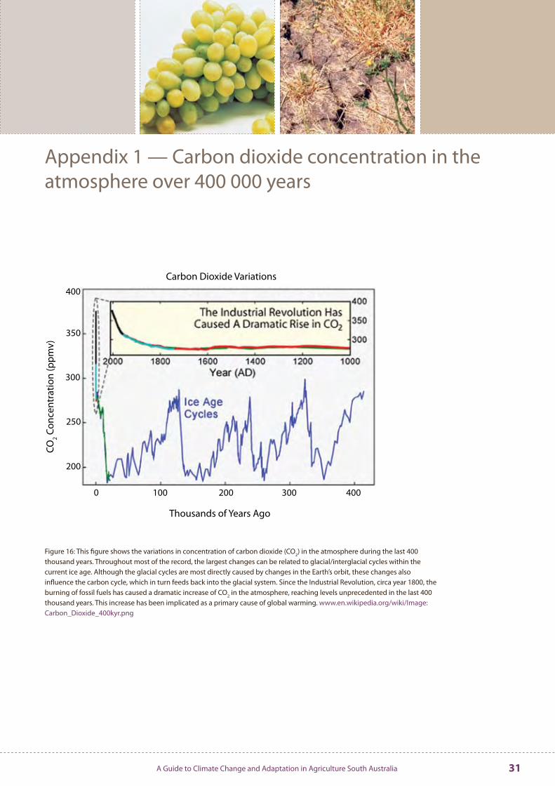
A Guide to Climate Change and Adaptation in Agriculture South Australia 31
Appendix 1 — Carbon dioxide concentration in the atmosphere over 400 000 years
Figure 16: This figure shows the variations in concentration of carbon dioxide (CO2) in the atmosphere during the last 400 thousand years . Throughout most of the record, the largest changes can be related to glacial/interglacial cycles within the current ice age . Although the glacial cycles are most directly caused by changes in the Earth’s orbit, these changes also influence the carbon cycle, which in turn feeds back into the glacial system . Since the Industrial Revolution, circa year 1800, the burning of fossil fuels has caused a dramatic increase of CO2 in the atmosphere, reaching levels unprecedented in the last 400 thousand years . This increase has been implicated as a primary cause of global warming . www .en .wikipedia .org/wiki/Image:Carbon_Dioxide_400kyr .png
Carbon Dioxide Variations
CO2 C
once
ntra
tion
(ppm
v)
Thousands of Years Ago
A Guide to Climate Change and Adaptation in Agriculture South Australia32
Policy timeline
1979 First World Climate Conference
1988 Intergovernmental Panel on Climate Change (IPCC) established to assess technical climate change issues, drawing together input from thousands of scientists around the world
1989 Representatives from 68 industrialised countries agree that stabilisation of carbon dioxide emissions by industrialised countries should be achieved as soon as possible in the ‘Noordwijk Declaration’
1990 Second World Climate Conference IPCC presents its first assessment report, providing broad scientific consensus that the possibility of climate change should be taken seriously
1992 United Nations Framework Convention on Climate Change (FCCC) signed in Rio de Janeiro by 155 countries, including Australia
Australia commits to provide a regularly updated national greenhouse gas inventory and reports on national policies and strategies for stabilising emissions
Council of Australian Governments (COAG) agrees on the National Greenhouse Response Strategy
1994 Framework Convention on Climate Change ratified by 50 countries, and comes into force as international law
1995 Intergovernmental Panel on Climate Change second assessment report released
1997 Development of Kyoto Protocol completed
Just prior to Kyoto, Australia launches a 5-year $180 million package of greenhouse initiatives and measures, including legislative mechanisms mandating that electricity generating companies source an additional 2% of power from renewable sources
Australia establishes the National Carbon Accounting System
1998 USA and Australia sign (but do not subsequently ratify) the Kyoto Protocol, which includes provisions for Australia to restrict emissions to 108% of 1990 levels by the end of the first commitment period (2008–2012)
Australian Greenhouse Office established and National Greenhouse Strategy developed, focussing on improving awareness and understanding, limiting greenhouse emissions and enhancing emission sink capacity, and developing adaptation responses
2001 IPCC third assessment report released
Australian Greenhouse Office releases a paper on Pathways and policies for the development of a national emissions trading system for Australia
2006 South Australian strategic plan for reducing greenhouse emissions released
2006 South Australia introduces a Climate Change and Greenhouse Emissions Reduction Bill 2006 into Parliament (including provisions for ‘voluntary offset programs’, the development of targets for ‘various sections of the State’s economy’ and the development of policies and programs for the reduction of greenhouse gas emissions)
Other documents prepared in 2006 include:
National Agriculture and Climate Change Action Plan for 2006–2009 — Australian Natural Resource Management Ministerial Council
National Climate Change Adaptation Framework — Council of Australian Governments (COAG)
Tackling Climate Change — South Australia’s Greenhouse Strategy
Possible Design for a National Greenhouse Gas Emissions Trading Scheme — National Emissions Trading Taskforce, Australian State and Territory Governments
2007 The three sections of the IPCC Fourth Assessment Report will be released in stages from February 2007
Appendix 2 — History of International and Australian policy on climate change

For further information regarding South Australian Government policy, please refer to:
Tackling Climate Change: South Australia’s Draft Greenhouse Strategy (2006)
The State Natural Resources Management Plan (2006)
Soil Conservation and Land Management Directions for the Agricultural Lands of South Australia (2004)
The State Food Plan (2004–2007) and industry plans
The Kyoto Protocol
Under the Kyoto Protocol, ‘Annex 1’ countries agreed to reduce overall global greenhouse emissions to 5.2% below 1990 levels by the end of the first commitment period (2008–2012). Signatory countries have differing targets (as set out in Annex B of the protocol), with the sum of the different targets producing a 5.2% global reduction. Mechanisms such as ‘emissions trading’, ‘clean development mechanisms’ and ‘joint implementation’ can be used to reduce emissions and Annex 1 countries can carry forward unused emissions allowances from one commitment period to the following period.
A Potential Greenhouse Gas Emission Trading Scheme
Greenhouse gas emissions trading has been suggested as an effective mechanism for reducing Australia’s emissions, probably by legislating to limit the total amount of greenhouse gases that may be produced by specified sectors and allowing companies within those sectors to buy and sell rights to emit greenhouse gases. Companies producing less emission (or less greenhouse gas) could sell their emission
rights while companies producing more would have to buy extra rights to emit extra greenhouse gases. Companies that develop more ‘greenhouse friendly’ production systems would gain an advantage over others.
If an emissions trading scheme is introduced, the Australian Greenhouse Office recognises the need to address the following issues in the design of any such scheme:
Accounting for emissions resulting from combustion, such as those from power stations and transport, is relatively straightforward, but accounting for other emissions sources, such as agriculture, (which comprises up to 35% of total emissions) can be much more complex.
The costs of developing and running an emissions trading system (including administration, monitoring and reporting costs) needs to be minimised.
A phasing-in period with transitional arrangements seems necessary for Australia’s energy intensive industries, but Australia is sensitive to any global reaction to this because of our large export trade (5).
For South Australian agriculture to be included in emissions trading on a non-voluntary basis, an emissions trading scheme would need to be developed (or an emissions trading scheme signed on to by Australia or South Australia) and legislation enacted, capping emissions in the agricultural sector.
The National Emissions Trading Task Force (2006) reported that recent modelling by McLennan Magasanik Associates estimates that the cost of emission permits would range from $5 to $35 per tonne of carbon dioxide emitted,
•
•
•
depending on the level of the cap and the rate of development of emission reducing technologies.
Source: McLennan Magasanik Associates (2006). The Economic Impacts of a National Emissions Trading Scheme on Australia’s electricity markets, http://www.emissionstrading.net.au/__data/assets/pdf_file/2019/Discussion_Paper_-_Ch_6_-_Estimated_impacts.pdf
33A Guide to Climate Change and Adaptation in Agriculture South Australia
