a friendly guide to wavelets || introduction to wavelet electromagnetics

Chapter 9

Introduction to Wavelet Electromagnetics

Summary: In this chapter, we apply wavelet ideas to electromagnetic waves, i.e., solutions of Maxwell's equations. This is possible and natural because Maxwell's equations in free space are invariant under a large group of symmetries (the conformal group of space-time) that includes translations and dilations, the basic operations of wavelet theory. The structure of these equations also makes it possible to extend their solutions analytically to a certain domain T C C 4 in complex space-time, which renders their wavelet representation particularly simple. In fact, the extension of an electromagnetic wave to complex space-time is already its wavelet transforms, so no further transformation is needed beyond analytic continuation! The process of continuation uniquely determines a family of electromagnetic wavelets tyz, labeled by points z in the complex space-time T. These points have the form z = x + zy, where x G R 4

is a point in real space-time and y belongs to the open cone V' consisting of all causal (past and future) directions in R 4 . S&z itself is a matrix-valued solution of Maxwell's equations, representing a triplet of electromagnetic waves. This triplet is focused at the real space-time point x — Rez £ R4 , and its scale, helicity, and center velocity are vested in the imaginary space-time vector y = Imz € V. An arbitrary electromagnetic wave can be represented as a superposition of wavelets \£z parameterized by certain subsets of T, for example, the set E of all points with real space and imaginary time coordinates called the Euclidean region. Such wavelet representations make it possible to design electromagnetic waves according to local specifications in space and scale at any given initial time.

Prerequisites: Chapters 1 and 3. Some knowledge of electromagnetics, complex analysis, and partial differential equations is helpful in this chapter.

9.1 Signals and Waves

Information, like energy, has the remarkable (and very fortunate!) property that it can repeatedly change forms without losing its essence. A "signal" usually refers to encoded information, such as a time-variable amplitude or frequency modulation imprinted on an electromagnetic wave acting as a "carrier." The information is taken for a "ride" on the wave, at the speed of light, to be decoded later by a receiver. Many of the most important signals do, in fact, have to ride an electromagnetic wave at some stage in their journey. But this ride may not be entirely free, since electromagnetic waves are subject to the physical laws of propagation and scattering. The effects of these laws on communication are often ignored in discussions of signal analysis and processing. But the physical

G. Kaiser, A Friendly Guide to Wavelets, Modern Birkhäuser Classics, DOI 10.1007/978-0-8176-8111-1_9, © Gerald Kaiser 2011

203

204 A Friendly Guide to Wavelets

laws are, in some sense, a code in themselves - in fact, an unchangeable, absolute code. Therefore it would seem that an understanding of the interaction between the two codes (the physical laws and the encoded information) can be helpful. In the transmission phase, it may suggest a preferred choice of both carrier and code. In the reception phase, it may suggest better decoding methods that take full advantage of the nature of the carrier and use it to understand the precise impact of the "medium" on the "message." This is especially important when the medium is the message, as it can be, for example, in optics and radar. In these cases, the initial signal is often trivial (for example, a spot light) and the information sought by the receiver is the distribution and nature of reflectors, absorbers, and so on.

In order to arrange a marriage between signal analysis and physics, it is first necessary to formulate both in the same language or code. For signals, this means any choice of scheme for analysis and synthesis. For electromagnetic waves, the "code" consists of the laws of propagation and scattering, so we have little choice. It therefore makes sense to begin with the physics and try to reformulate electromagnetics in a way that is most suitable for signal analysis. The two themes for signal analysis explored in this book have been time-frequency and time-scale analysis. In this chapter we will see that the propagation of electromagnetic waves can be formulated very naturally in terms of a generalized time-scale analysis. In fact, the laws of electromagnetics uniquely determine a family of wavelets that are specifically dedicated to electromagnetics. These wavelets already incorporate the physical laws of propagation, and they can be used to construct arbitrary electromagnetic waves by superposition. Since the physical laws are now built into the wavelets, we can concentrate on the "message" in the synthesis stage, i.e., when choosing the coefficient function for the superposition. The analysis stage consists of finding a coefficient function for a given wave; again this isolates the message by displaying the informational contents of the wave.

Time-scale analysis is natural to electromagnetics for the following fundamental reason: Maxwell's equations in free space are invariant under a group of transformations, called the conformal group C, which includes space-time translations and dilations. That is, if any solution is translated by an arbitrary amount in space or time, then it remains a solution. Similarly, a solution can be scaled uniformly in space-time and still remain a solution. Since these are precisely the kind of operations used to construct wavelet analysis, it is reasonable to expect a similar analysis to exist for electromagnetics. The other ingredient in the construction of ordinary wavelet analysis is the Hilbert space L2(R), chosen somewhat arbitrarily. Translations and dilations were represented by unitary operators on L2(R), and the wavelets formed a (continuous or discrete) frame in L2(R). In the case of electromagnetics, we need a Hilbert space 7i consisting

9. Introduction to Wavelet Electromagnetics 205

of solutions of Maxwell's equations instead of unconstrained functions (such as those in L2(R)).

But we must not blindly apply the "hammer" of wavelet analysis to this new "nail" Hj since this nail actually (and not surprisingly) turns out to have much more structure than L2(R). It is, in fact, more like a screw than a nail! The extra structure is related to the other symmetries contained in the conformal group C. Besides translations and dilations, C contains rotations, Lorentz transformations, and special conformal transformations. In fact, these transformations taken together essentially characterize free electromagnetic waves: It is possible to begin with C and construct H as a representation space for C, where conformal transformations act as unitary operators (Bargmann and Wigner [1948], Gross [1964]). When constructing a wavelet-style analysis for electromagnetics, it is important to keep in mind that most of the standard continuous analysis-synthesis schemes are completely determined by groups. In Fourier analysis, the group consists of translations (Katznelson [1976]). In windowed Fourier analysis, it is the Weyl-Heisenberg group W consisting of translations, modulations and phase factors (Folland [1989]). In ordinary wavelet analysis, it is the affine group A consisting of translations and dilations (Aslaksen and Klauder [1968, 1969]). Since both W and A contain translations, the associated analyses are related to Fourier analysis but contain more detail. The extra detail appears in the parameters labeling the frame vectors: The (unnormalizable) "frame vectors" ew{t) = e2ntut in Fourier analysis are parameterized only by frequency; the frame vectors gWit of windowed Fourier analysis are parameterized by frequency and time, and the frame vectors tpSit of ordinary wavelet analysis are parameterized by scale and time. Since the conformal group C contains A, we expect that the electromagnetic wavelet analysis will be related to, but more detailed than, the standard wavelet analysis. In fact, its frame vectors will be seen to be electromagnetic pulses *&z parameterized by points z = x + iy in a complex space-time domain T C C4 , thus having eight real parameters. The real space-time point x = (x, t) G R4 represents the focal point of Sfrz. This means that at times prior to t, \£2 converges toward the space point x, and at later times it diverges away from x. At time £, \I/z is localized around x £ R3 . Since it is a free electromagnetic wave, it does not remain localized. But it does have a well-defined center that is described by the other half of z, the imaginary space-time vector y — (y, s). y must be causal, meaning that |y| < c|s|, where

* I am thinking of the wonderful saying: If the only tool you have is a hammer, then everything looks like a nail. Until recently, of course, the only tool available to most signal analysts was the Fourier transform or its windowed version, so everything looked like either time or frequency. Now some wavelet enthusiasts claim that everything is either time or a scale.


c is the speed of light, and it has the following interpretation: v = y / s is the velocity of the center of \£z, and \s\ is the time scale (duration) of \I/z. Equiv-alently, c\s\ is the spatial extent of \PZ at its time of localization t. The sign of the imaginary time 5 is interpreted as the helicity of *$>z, which is related to its polarization.

In Section 9.2 we solve Maxwell's equations by Fourier analysis. Solutions are represented as superpositions of plane waves parameterized by wave number and frequency. We define a Hilbert space H of such solutions by integration over the light cone in the Fourier domain. In Section 9.3 we introduce the analytic-signal transform (AST). This is simultaneously a generalization to n dimensions of two objects: the ordinary wavelet transform, and Gabor's idea of "analytic signals." The AST extends any function or vector field from R n to C n , and we call the extended function the analytic signal of the original function. In general, such analytic signals are not analytic functions since there may not exist any analytic extensions. We prove that the analytic signal of any solution in H is analytic in a certain domain T c C 4 , the causal tube. This analyticity is due to the light-cone structure of electromagnetic waves in the Fourier domain, just as the analyticity of Gabor's one-dimensional analytic signals is due to their having only positive-frequency components. In Section 9.4 we use the analytic signals of solutions to generate the electromagnetic wavelets \I>Z. We derive a resolution of unity in H in terms of these wavelets, which gives a means of writing an arbitrary electromagnetic wave in H as a superposition of wavelets. In Section 9.5 we compute the wavelets explicitly, which also gives their reproducing kernel. In Section 9.6 this explicit form of ^z is used to give the wavelet parameters z =■ x + iy a complete physical and geometric interpretation, as explained above. In Section 9.7 we show how general electromagnetic waves can be constructed from wavelets, with initial data specified locally and by scale.

The wavelet analysis of electromagnetics is based entirely on the homogeneous Maxwell equations. Acoustic waves, on the other hand, obey the scalar wave equation, which has a very similar structure to Maxwell's equations in that its symmetry group is the same conformal group C. Therefore a similar wavelet analysis exists for acoustics as well as for electromagnetics. In the language of groups, the two analyses are just different representations of C. Acoustic wavelet representations and the corresponding wavelets ^ J are studied in Chapter 11.

9.2 Fourier Electromagnetics

An electromagnetic wave in free space (without sources or boundaries) is described by a pair of vector fields depending on the space-time variables x = (x, XQ), namely, the electric field E(x) and the magnetic field B(x). (Here x is


the position and XQ = t is the time.) These are subject to Maxwell's equations,

V x E + <90B = 0, V • E = 0,

V x B - 5 b E = 0, V • B = 0,

where V is the gradient with respect to the space variables and do is the time derivative. We have set the speed of light c = 1 for convenience. The parameter c may be reinserted at any stage by dimensional analysis. In keeping with the style of this book, we are not concerned here with the exact nature of the "functions" E(x) and B(x) (they may be regarded as tempered distributions; see Kaiser [1994c]). Note tha t the equations are symmetric under the linear mapping defined by J : E i—► B , B H —E, and tha t J 2 is minus the identity map. This means tha t J is a "90°-rotation" in the space of solutions, analogous to multiplication by i in the complex plane. Such a mapping on a real vector space is called a complex structure. The combinations B ± i E diagonalize J , since J ( B ± « E ) = ±i (B ± iE). They each map Maxwell's equations to a form in which the concepts of helicity and polarization become very simple. It will suffice to consider only F = B + i E , since the other combination is equivalent. Equations (9.1) then become

d0F = zV x F , V • F = 0. (9.2)

Note tha t the first of these equations is an evolution equation (initial-value problem), while the second is a constraint on the initial values. Taking the divergence of the first equation shows tha t the constraint is conserved by time evolution. Note also tha t it is the factor i in (9.2) (i.e., the complex structure) tha t couples the t ime evolution of the electric field E to tha t of the magnetic field B . Equation (9.2) implies

-<92F = V x (V x F ) = V ( V • F ) - V 2 F = - V 2 F (9.3)

in Cartesian coordinates, hence the components of F become decoupled and each satisfies the wave equation

D F E E ( - d g + V 2 ) F = 0. (9.4)

To solve (9.2), write F as a Fourier transform*

F(x) = ( 27T)" 4 / dApeipxF(p), (9.5)

t In this chapter we change our convention for Fourier transforms. The four-vector p now denotes wave number and frequency in radians per unit length or unit time. Also, we are identifying R 4 with its dual R4 by means of the Lorent-invariant inner product, so the pairing between x and p is expressed as an inner product. See the discussion in Section 1.4.


where p — (p,Po) € R 4 with p G R 3 as the spatial wave vector and po as the frequency. We use the Lorentz-invariant inner product

p • x = poxo - p • x.

(Note also that we have reverted to the convention for the Fourier transform with the 2TT factors in front of integrals instead of in the exponents. This is the convention used in the physics literature.) The wave equation (9.4) implies tha t p2F(p) = 0, where

2 2 i i2

P =P'P = P0-\P\ • Thus F must be supported on the light cone C = {p : p2 = 0,p / 0}* shown in Figure 9.1, i.e., on

C = {(p,po) 6 R 4 : Pi = | p | 2 , P ^ 0} = C+ U C.

C+ = {(p,po) : Po = |p | > 0} = positive-frequency light cone (9.6)

C_ = {(p,po) : Po — ~|p| < 0} = negative-frequency light cone.

p0 (frequency)

p-plane

F igure 9 .1 . The positive- and negative-frequency cones V± and their boundaries, and the positive- and negative-frequency light cones C± = dV±.

Hence F has the form F(p) = 27r<5(p2)f(p),

where f : C -* C 3 is a function on C or, equivalently, the pair of functions on R 3 given by

f±(p) = f ( p » i ^ ) j where u = | p |

t We assume that the fields decay at infinity, so F(p) contains no term proportional to 6{p), i.e., F(x) has no "DC component." To eliminate this possibility, we exclude p = 0 from the light cone.

(9.8)


is the absolute value of the frequency. But

Stf) = S((P0 - w ) ( p o + w ) ) = % ° - « H - ' ( * » + "> . (9.7)

Hence (9.5) becomes

F(x) = ( 2 ^ r 3 / ^ H . e-ip-x [ e- t f + ( p ) + e - ic t f _ ( p ) ]

= [ dpeipxf(p), Jc

where dp = (27r)"3d3p/2u;

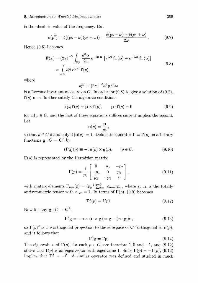
is a Lorentz-invariant measure on C. In order for (9.8) to give a solution of (9.2), f (p) must further satisfy the algebraic conditions

ipof(p) = p x f ( p ) , p-f(p) = 0 (9.9)

for all p G C , and the first of these equations suffices since it implies the second. Let

n(p) = £ , so that p e C if and only if |n(p)| — 1. Define the operator T = T(p) on arbitrary functions g : C —► C 3 by

(r g)(p) = - i n(p) x g(p), p G C . (9.10)

r (p) is represented by the Hermitian matrix

T(p) = -L 0 p3 - p 2 ]

-P3 0 P! , (9.11) L P2 - P I o J

with matrix elements Tmn(p) = zp^1 £) f c = 1 £mnkPk , where £mnfc is the totally antisymmetric tensor with £123 = 1. In terms of T(p), (9.9) becomes

rf(p) = f(p). (9.12)

Now for any g : C -» C3 ,

r 2 g = - n x (n x g) = g - (n • g)n , (9.13)

so T(p)2 is the orthogonal projection to the subspace of C 3 orthogonal to n(p), and it follows that

r 3g = r g . (9.14)

The eigenvalues of T(p), for each p 6 C, are therefore 1,0 and —1, and (9.12) states that f(p) is an eigenvector with eigenvalue 1. Since T(p) = —T(p), (9.12) implies that r f = — f. A similar operator was defined and studied in much


more detail by Moses (1971) in connection with fluid mechanics as well as electrodynamics.

Consider a single component of (9.8), i.e., the plane-wave solution

Fp(x) = e*'* f (p) = Bp(x) + iE p (x) , (9.15)

with arbitrary but fixed p G C and f (p) ^ 0. The electric and magnetic fields are obtained by taking the real and imaginary parts. Now T(p) f (p) = f (p) and r(p)f(p) = - f 5 ) imply

T(p)Fp(x) = Fp(x), r(p)Fp(aO = - F p ( x ) . (9.16)

Since T(p)* = T(p), these eigenvectors of T(p) with eigenvalues 1 and —1 must be orthogonal:

Fp(x)*Fp(x) = Fp(x) • Fp(x) = 0, where the asterisk denotes the Hermitian transpose. Taking real and imaginary parts, we get

|Bp(x)|2 = |Ep(z) |2 , Bp(x) ■ Ep{x) = 0. (9.17) The first equation shows that neither Bp(z) nor Ep(x) can vanish at any x (since f(p) zfz 0). Furthermore, (9.16) implies that

pxEp(r r ) =p0Bp(x).

Thus, for any x, {p, Ep(x),Bp(:r)} is a right-handed orthogonal basis if po > 0 (i.e., p G C+) and a left-handed orthogonal basis if po < 0 (p G C_). Taking the real and imaginary parts of (9.15) and using f(p) = Bp(0) + zEp(0), we have

Bp(x) = cos(p • x)Bp(0) - sin(p • x)Ep(0), ^ Ep(x) = cos(p • x)Ep(0) + sin(p • x)Bp(0).

An observer at any fixed location x G R 3 sees these fields rotating as a function of time in the plane orthogonal to p. If p G C+, the rotation is that of a right-handed corkscrew, or helix, moving in the direction of p, whereas if p G C_, it is that of a left-handed corkscrew. Hence Fp(x) is said to have positive helicity if p G C+ and negative helicity if p G C_.

A general solution of the form (9.8) has positive helicity if f(p) is supported in C+ and negative helicity if f(p) is supported in C_. Other states of polarization, such as linear or elliptic, are obtained by mixing positive and negative helicities. The significance of the complex combination F(x) — B(x) + iE(x) therefore seems to be that, in Fourier space, the sign of the frequency po gives the helicity of the solution! (Usually in signal analysis, the sign of the frequency is not given any physical interpretation, and negative frequencies are regarded as a necessary mathematical artifact due to the choice of complex exponentials over sines and cosines.) In other words, the combination B + zE "polarizes"


the helicity, with positive and negative helicity states being represented in C+

and C- , respectively. Had we used the opposite combination B — i E , C+ and C- would have parameterized the plane-wave solutions with opposite helicities. Nothing new seems to be gained by considering this alternative.t

In order to eliminate the constraint, we now proceed as follows: Let

n(p) = | [r(p) + r2(P)]. (9.19)

Explicitly,

n (p) = 0 o

Po-Pi -PlP2 + «P0P3 ~PlP3 ~ IP0P2

PI-PI -P1P2 - IP0P3

L ~PlP3 + ^P0P2 -P2P3 - *PoPl

-P2P3 + IPOPI

PI-PI (9.20)

The established properties T* =T = T3 imply tha t II* = II = I I 2 and T i l = II, which proves tha t II(p) is the orthogonal projection to eigenvectors of T(p) with eigenvalue 1. Thus, to satisfy the constraint (9.12), we need only replace the constrained function f (p) in (9.8) by II(p)f (p), where f (p) is now unconstrained.

P r o p o s i t i o n 9 .1 . Solutions of Maxwell's have the following Fourier representation:

Jc (9.21)

with f : C —* C 3 unconstrained.

Consequently, the mapping f i—► F is not one-to-one since II is a projection operator. In fact, f is closely related to the potentials for F , which consist of a real 3-vector potential A(x) and a real scalar potential AQ{X) such tha t

B = V x A, E = -d0A - VA0. (9.22)

The combination (A(x) , Ao(x)) is called a "4-vector potential" for the field. We can assume without loss of generality tha t the potential satisfies the Lorentz condition (Jackson [1975])

V • A + d0A0 = 0.

* Maxwell's equations are invariant under the continuous group of duality rotations, of which the complex structure J mapping E to B and B to —E is a special case. In the complexified solution space, the combinations B ± i E form invariant subspaces with respect to the duality rotations. That gives the choice of B + *E an interpretation in terms of group representation theory.


Since A and Ao also satisfy the wave equation (9.4), they have Fourier representations similar to (9.8):

A(x) = f dp eipx8i{p), A0(x) = f dp eipxa0(p). (9.23) Jc Jc

The Lorentz condition means that poao(p) = p • a(p), or ao(p) = n • a(p), so ao is determined by a. Equations (9.22) will be satisfied provided that the Fourier representatives e(p)1 b(p) of E , B satisfy

b = - i p x a = p 0 r a , e = -ipoa + i pa0 = —ipo T2 a. (9.24)

Hence F = B + i E is represented in Fourier space by

b(p) + ie(p) = po [T(p) + T(p)2] a(p) = 2p0U(p) a(p). (9.25)

This shows that we can interpret the unconstrained function f(p) in (9.21) as being directly related to the 3-vector potential by

f(p) = 2poa(p), (9.26)

modulo terms annihilated by II (p), which correspond to eigenvalues —1 and 0 of T(p). Viewed in this light, the nonuniqueness of f in (9.21) is an expression of gauge freedom in the B + i E representation, as seen from Fourier space. In the space-time domain, (B, E) are the components of a 2-form F in R4 and (A, AQ) are the components of a 1-form A. Then equations (9.1) become dF = 0 and SF = 0 (where 6 is the divergence with respect to the Lorentz inner product), Equations (9.22) become unified as F = dA, the Lorentz condition reads 8A = 0, and the gauge freedom corresponds to the invariance of F under A —> A + dx, where x(x) is a scalar solution of the wave equation.

Maxwell's equations are invariant under a large group of space-time transformations. Such transformations produce new solutions from known ones by acting on the underlying space-time variables (possibly with a multiplier to rotate or scale the vector fields). Some trivial examples are space and time translations. Obviously, a translated version of a solution is again a solution, since the equations have constant coefficients. Similarly, a rotated version of a solution is a solution. A less obvious example is Lorentz transformations, which are interpreted as transforming to a uniformly moving reference frame in space-time. (In fact, it was in the study of the Lorentz invariance of Maxwell's equations that the Special Theory of Relativity originated; see Einstein et al. (1923).) The scale transformations x —* ax, a ^ 0, also map solutions to solutions, since Maxwell's equations are homogeneous in the space-time variables. Finally, the equations are invariant under "special conformal transformations" (Bate-man [1910], Cunningham [1910]), which can be interpreted as transforming to a uniformly accelerating reference frame (Page [1936]; Hill [1945, 1947, 1951]).


Altogether, these transformations form a 15-dimensional Lie group called the conformal group, which is locally isomorphic to 5C7(2, 2) and will here be denoted by C. Whereas wavelets in one dimension are related to one another by translations and scalings, electromagnetic wavelets will be seen to be related by conformal transformations, which include translations and scalings. (A study of the action of SU(2, 2) on solutions of Maxwell's equations has been made by Riihl (1972).)

To construct the machinery of wavelet analysis, we need a Hilbert space. That is, we must define an inner product on solutions. It is important to choose the inner product to be invariant under the largest possible group of symmetries since this allows the largest set of solutions in H to be generated by unitary transformations from any one known solution. (In quantum mechanics, invariance of the inner product is also an expression of the fundamental invariance of the laws of nature with respect to the symmetries in question.) Let f (p) satisfy (9.12), and let a(p) be a vector potential for f satisfying the Lorentz condition so that the scalar potential is determined by ao(p) — n(p) • a(p). By (9.25),

|f (p)\2 = 4p2 \U(p) a(p)|2 = 4a;2 a(p) • U(p) a(p)

= 2UJ2 a(p) • T(p) a(p) + 2LJ2 a(p) • T(p)2 a(p).

The first term is

(9.27)

-2icj2 a(p) • (n x a(p)) = 2iu2 n • (a(p) x a(p)), (9.28)

which cancels its counterpart with p —> — p on account of the reality condition a(~~p) — a(p)- Thus

% |f (p)|2 = 2 f dp Kp)- [a(p) - n(n • a(p))] w Jc c v Jc

= 2 I dp Jc

|a(p)|2-|ao(p)|^ (9.29)

The integrand in the last expression is the negative of the Lorentz-square of the 4-potential (a(p),ao(p)). Consequently, the integral can be shown to be invariant under Lorentz transformations. (Note that |a|2 — |ao|2 > 0, vanishing only when a(p) is a multiple of p, in which case f = 0. This corresponds to "longitudinal polarization.") Hence (9.29) defines a norm on solutions that is invariant under Lorentz transformations as well as space-time translations. In fact, the norm (9.29) is uniquely determined, up to a constant factor, by the requirement that it be so invariant. Moreover, Gross (1964) has shown it to be invariant under the full conformal group C. Again we eliminate the constraint by replacing f (p) with II(p) f(p). Thus, let Ji be the set of all solutions F(x)


defined by (9.21) with f : C —► C 3 square-integrable in the sense that

| |F| |2=/§|n(p)f(P) |2

f * (9-3°) = ( 2 T ) _ 3 i ; l ^ | n ( p ) f ( p ) | 2 < T O -7i is a Hilbert space under the inner product obtained by polarizing the norm (9.30) and using (Ilf)*IIg = f*ITIIg = f*IIg.

Definition 9.2. H is the Hilbert space of solutions (9.21) with inner product

(P,G>=/^-f(prn(p)g(p). (9.31)

7i will be our main arena for developing the analysis and synthesis of solutions in terms of wavelets. Note that when (9.12) holds and f±(p) = f (p, ±CL>) are continuous, then

f(0) = f±(0) = 0 (9.32) must hold in order for (9.30) to be satisfied. This is a kind of admissibility condition that applies to all solutions in H: There must not be a "DC component." In fact, the measure d 3 p / | p | 3 is a three-dimensional version of the measure df/|£| that played a role in the admissibity condition of one-dimensional wavelets.

To show the invariance of (9.30) under conformal transformations, Gross derived an equivalent norm expressed directly in terms of the values of the fields in space at any particular time XQ = t:

\\F\\k0ss = 4 / £ ^ J - F(x,t)'F(y,t). (9.33) " J R 6 IX yi

The right-hand side is independent of t due to the invariance of Maxwell's equations under time translations (which is, in turn, related to the conservation of energy). A disadvantage of the expression (9.33) is that it is nonlocal since it uses the values of the field simultaneously at the space points x and y. In fact, it is known that no local expression for the inner product can exist in terms of the field values in (real) space-time R 4 (Bargmann and Wigner [1948]). In Section 4, we derive an alternate expression for the inner product directly in terms of the values of the electromagnetic fields, extended analytically to complex space-time. This expression is "local" in the space-scale domain (rather than in space alone). But first we must introduce the tool that implements the extension to complex space-time.


9.3 The Analytic-Signal Transform

We now introduce a multidimensional generalization of the wavelet transform that will be used below to analyze electromagnetic fields. To motivate the construction, imagine that we have a (possibly complex) vector field F : R 4 —► C m

on space-time. For example, F could be an electromagnetic wave (in which case m = 3 and F is given by (9.21)), but this need not be assumed. Suppose we want to measure* this field with a small instrument, one that may be regarded as a point in space at any time. Suppose further that the impulse response of the instrument is a (possibly) complex-valued function h : R —► C. If the support width of h is small, then we can assume that the velocity of the instrument is approximately constant while the measurement takes place. Then the trajectory on the instrument in space-time may be parameterized as

x(r) = x + ry, i.e., ( x ( r ) = X + ^ (9.34)

where x = (x, xo) G R 4 is the "initial" point and y = (y, yo) is "velocity." The actual three-dimensional velocity in space is

v = 1- , (9.35)

so we require

| v | < c , i.e., \y\<c\y0\. (9.36) We model the result of measuring the field F with the instrument h, moving along the above trajectory, as

/

co drh(r)F(x + ry). (9.37)

-co

This is a multidimensional generalization of the wavelet transform (Kaiser [1990a, b]; Kaiser and Streater [1992]). To see this, suppose for a moment that we replace space-time by time alone, and the field is scalar-valued, i.e., F : R —> C. Then x,y G R and (9.36) reduces to y ^ 0. By changing variables in (9.37), the transform becomes

Fh(x,y) = J°°duy-h (j—^\ F(u). (9.38)

* I do not claim that this is a realistic description of electromagnetic field measurement. It is only meant to motivate the generalized wavelet transforms developed in this section by relating them to the standard wavelet transforms.


This is recognized as essentially identical to the usual wavelet transform, with the wavelets now represented by

W « ) ~ ^ ( ~ ) - (9-39)

(The symbol ~ instead of equality will be explained below.) In the one-dimensional case treated in Chapter 3, we assumed, without any particular reason, that F belonged to L2(R). Inspired by the electromagnetic norm (9.30), let us now suppose instead that F belongs to the Hilbert space

Ha = {F : \\F\\l < oo}, where \\F\\l = ± | ~ ^ |F(p)|2 (9.40)

for some a > 0. The inner product in Ha is obtained, as usual, by polarizing the expression for | |F| |^. Battle (1992) calls H.2a a "massless Sobolev space of degree a." We now derive a reconstruction formula for this case to prepare ourselves for the more complicated case of electromagnetics. The main points of interest in this "practice run" are the modifications forced on the definition of the wavelets and the admissibility condition by the presence of the weight factor \p\~a in the frequency domain. Since

jye~tpu¥\h(^)=e~ipxHpy)' (9-4i) Parseval's formula applied to (9.38) gives

/

CO _

dp e^ h(py)F(p) -oo

= Wl fl ^ \p\ae'px h(py)F(p) (9-42)

= \ 'lx,y i r /a = "-ay r ,

where Kv(p) = \v\ae-ipxh{vy)- (9-43)

This shows that the wavelets are given in the time domain by

1 C°° hXtV(u) = — y_ dp |Pre*<"-*> h(py). (9.44)

If we take a = 0, then Ha = L2(R) and (9.44) reduces to (9.39). For a > 0, (9.39) is not valid. (That explains the symbol ~ in (9.39).) Now let us see how to reconstruct F from its transform Fh- Applying Plancherel's formula to (9.42) gives

/

oo /»oo

dx \Fh(x,y)f = (27T)-1 / dp \h(py)\2\F(p)f. (9.45) -oo J — oo


Integrating both sides over y with the weight function |?/|Q_1 gives

/

OO rOO

dx / dy\yrl\Fh(x,y)\2

~oo J — oo

= (27T)"1 f° dp |F(p)|2 f ° dy I J / I - 1 Iftfpy)!2 (9-46) J—oo J— oo

where we have changed y to £ = py, and let

/

oo

<*£ K M W . (9.47) -oo

which now is assumed to be finite. Therefore we define an inner product for transforms by

/

OO /•OO

dx / dy\y\°-1Fh(x,y)Gh(x,y) , r r (9.48)

/ dx / d i / M ^ F ' ^ . y ^ G , J — oo J — oo

Ot f — oo

so that (9.46) becomes a Plancherel-type relation | | i^ | | 2 = ||^||a? a n d by polarization,

(Fh,Gh)=F*G. (9.49) This means that (9.48) gives a resolution of unity:

/

OO /"OO

dx / dy \y\a~l hXtV h^y = I weakly in Ha . (9.50) -oo J — oo

As usual, this means that vectors in Ha can be expanded in terms of the wavelets hX)V , and all the theorems in Chapter 4 apply concerning the consistency condition for transforms, least-squares approximations, and so on. Note that the admissibility condition is now Ca < oo, which reduces to the usual admissibility condition only when a = 0.

Having explained the relation of (9.37) to the usual one-dimensional wavelet transform, we now return to the four-dimensional case. Inserting the Fourier representation of F, we obtain

Fh(x,y) = (2TT)-4 ^ dr h(r) f dfipeP'^+^Flp)

= ( 2 T T ) " 4 / d4peipxF{p) [ dreiTpyh{r) (9.51) Jn4 J-oo

= (2TT)-4 / d4pe^xl(p-y)F(p). Jn4

That is, Fh(x,y) is a windowed inverse Fourier transform of F(p), where the window in the Fourier domain is h(p • y). Note that all Fourier components


F(p) in a given three-dimensional hyperplane Pa = {p : p • y = a} are given equal weights by this window.* To construct wavelets from /i, as was done in the one-dimensional case by (9.44), we need an inner product on the vector fields F . This will be done in the next section, where the F ' s will be assumed to be electromagnetic waves. But now we specialize our transform by choosing

h(r) = — — . (9.52) iri r — %

With this choice, we denote F^(x , y) by ¥{x -f iy) and call it the analytic signal of F . We state the definition in the general case, where R 4 is replaced by R n .

Def in i t ion 9 .3 . The analytic signal o / F : R n -> C m is the function F : C n -> C m defined formally by

1 C°° rln-F(x + iy) = — / : F(x + ry). (9.53)

TTl J_00 T - I

The mapping F i - > F will be called the analytic-signal transform (AST).

In general F is not analytic, so it may actually depend on both z = x + iy and z = x — iy. The reason for the above notation will become clear below. By contour integration, we find

kS) = --j^—e-«T = 2e(t)eS, (9.54)

where 6 is the step function

r i ? > o tf(0 =1.5 ( = 0 (9.55)

I 0 £ < 0. Thus we have shown the following:

P r o p o s i t i o n 9.4. The analytic-signal transform is given in the Fourier domain by

F{x + iy) = (2TT)- 4 f d4p29{p • y) eip<x+iy"> F (p) . (9.56)

The factor 6(p • y) plays two important roles in (9.56):

* Equation (9.37) defines a one-dimensional windowed Radon transform. A similar transform can be defined modeled on field measurements where the instrument is assumed to occupy k < 3 space dimensions. (For a point instrument, k = 0; for a wire antenna, k = 1; for a dish antenna, k = 2.) This gives a k + 1-dimensional windowed Radon transform in R4 . See Kaiser (1990a, b), and Kaiser and Streater (1992).)


(a) Suppose that F(p) is absolutely integrable, so that F(x) is continuous. If the factor 9(p • y) were absent in (9.56), then e~py can grow without bounds, and the above integral can diverge unless F{p) happens to decay sufficiently rapidly to balance this growth. This option is not available for general electromagnetic waves in the Hilbert space W of Section 9.2, since there F(p) is supported in the light cone C = C+ U C_; so whenever p belongs to the support of F, then — p may possibly also belong to the support of F , and there is no reason for F to have the exponential decay required to make the integral converge.

(b) The factor 6{p • y) tends to spoil the analyticity of F. If this factor were absent, and the integral somehow converged, then the resulting function depends only on z = x + iy rather than on both z and z, and F(z) is analytic (formally, at least).

We will now show that under certain conditions, which hold in particular when F belongs to the Hilbert space TC, F(z) is indeed analytic, provided z is restricted to a certain domain T C C 4 in complex space-time. Again, we revert temporarily from four dimensions (space-time) to one dimension (time), in order to clarify the ideas. Suppose that F : R —► C is such that F(p) is absolutely integrable. Then (9.56) is replaced by

/

oo dp 2Q(py) e

ip(x+iy) F{p). (9.57) -oo

If y > 0, then 6{py) = 6{p) and />00

F(x + iy) = Tf-1 / dpeip{x+iy) F(p), y > 0. (9.58) Jo

The integral converges absolutely and, as z = x + iy varies over the upper-half z-plane, it defines an analytic function. Therefore F(z) is analytic in the upper-half plane C+, and for z € C+, F contains only positive-frequency components. Similarly, when y < 0, then 9(py) — 0(—p) and

f° F(x + iy) = 7T-1 / dpeip{x+iy) F(p), y<0. (9.59)

J — oo

F is analytic in the lower-half plane C_, and for z G C_, F(z) contains only negative-frequency components. Thus, F is analytic in C + U C_. It is not analytic on the real axis, in general. The relation between F(z) and the original function F(x) can be summarized as follows:

\ lim 2 y - o + L

POO

F(x + iy) + F(x -iy)\= (27r)_1 / dp eipx F(p) = F(x). (9.60)


Thus F(x) is a "two-sided boundary value" of F(z), as z approaches the real axis simultaneously from above and below. On the other hand, the discontinuity across R is given by

\ lim F(x + iy) - F(x - iy) \= (2TT)~1 / dp sign (p)eipx F(p) y^o+ L J J_00

= iHF(x), (9.61)

where H : L2(H) —► L2(H) is the Hilbert transform. When F is real, then F(z) = F(z) for all z and

F(x) = lim ReF(x + iy)

HF(x) = lim ImF(x + iy). (9.62)

For example,

F(x) = cosx => F(p)=7r8(p-l) + 7r6(p+l), (9.63)

so

elz, cos z, e~iz,

zeC+

zeK , z € C _

HF(x) = sinx. F{z) = { cosz, zeK , HF{x) = smx. (9.64)

The function F in (9.58) was introduced by Gabor (1946), who called it the analytic signal of F. It has proved to be very useful in optics, radar, and many other fields. (For optics, see Born and Wolf (1975), Klauder and Sudarshan (1968). For radar, see Rihaczek (1968); also Cook and Bernfeld (1967), where analytic signals are called "complex waves.") When F is real, then the Gabor analytic signal (defined in C+ only) suffices to determine F by (9.62), because the negative-frequency part of F is simply the complex conjugate of the positive-frequency part . When F is complex, the two parts are independent and both (9.58) and (9.59) are needed in order to recover F.

Our definition (9.53) is a generalization of Gabor 's idea to any number of dimensions and to functions tha t are not necessarily real-valued. Tha t explains the name "analytic-signal transform" given to the mapping F i—»• F in (9.53). To extend the relations (9.60) and (9.61) to the general case, we return to the original definition (9.53) with z = x+iey , 2 / ^ 0 , and consider its limit as £ —>• 0 + :


1 f°° C\T

lim Fix + ley) = — lim / F(x + ery) e^0+ 1TI e-+0+ J_OQ T — l

1 ,. f°° du „ , = — hm / Fix + uy)

7TI 6-^0+ J_00 U — IS

= — \iirF(x) + P / — F(x + uy)\ (9.65) ™ L J-oo u J

= F{x) + —P / — F(z + m/ 7TZ J_00 U

= F(x) + -P / — Ffr-uy), where P J • • • denotes the Cauchy principal value. The multivariate Hilbert transform in the direction of y =fi 0 is defined by

1 /*00 7

# y F(x ) = -P / — F(x - wy). (9.66)

It actually depends only on the direction of y, since

# a y F = sign (a) F y F , a ^ 0, (9.67)

so the usual definition (Stein [1970]) assumes that y is a unit vector with respect to an arbitrary norm in R n (which Stein takes to be the Euclidean norm). Since in our case R n = R4 is the Minkowskian space-time with the indefinite Lorentz scalar product, we prefer the unnormalized version. Equation (9.65) gives the generalizations of (9.60) and (9.61):

F(x) = - lim \F(X + ley) + F(x - iey)] \£-*0+[ _ _ J (9.68)

HvF(x) = — lim \F(X + iey) - Fix - iey)} . 2% e—►()+ L J

What about analyticity in the general case? Recall that for free electromagnetic waves, F(p) = <5(p2)f(p), s o F *s supported on the light cone C — {p : p2 = 0}. More generally, suppose F is supported inside the solid double cone

V = {p= (p l P 0 ) : p2 =p20 - c2 |p|2 > 0} = V+ U VL ,

y + = { p = ( p , p o ) : p o > c | p | } , (9.69) V_ = {p= (p,po) :p0 < - c | p | } ,

where we have temporarily reinserted the speed of light c. (This will clarify the difference between V± and their dual cones V±, to be introduced below.)


V+ is the positive-frequency cone and VL is the negative-frequency cone. The positive- and negative-frequency light cones are the boundaries of V± : C± = dV± C V±. (See Figure 9.1.) V± are both convex^ a property not shared by C±. (This means that arbitrary linear combinations of vectors in V± with positive coefficients also belong to V±.) The four-dimensional positive- and negative-frequency cones V± take the place of the positive- and negative-frequency axes in the one-dimensional case, i.e.,

V+ <-► {p G R : p > 0} = R+ , VI *-* {p G R : p < 0} = R_ . (9.70)

The dual cones of V+ and VL are defined by

V | = {y G R4 : p • y > 0 for all p G V+} V^ = {y G R 4 : p • j / > 0 for all p G VL}.

To find V\_ explicitly, let y G V+. Then we have

p • y = ujy0 - p • y > 0 for all p G V+ . (9.72)

If y = 0, then (9.72) implies y0 > 0. If y ^ 0, taking p = ujy/(c |y|) in (9.72) gives

c y o - | y | > 0 . (9.73)

This condition, in turn, is seen to be sufficient for y to belong to V+. If it holds, then by the Schwarz inequality in R3 ,

peV+ => p ■ y = ujy0 - p • y > ujy0 - |p| |y| = \p\(cy0 - |y|) > 0. (9.74)

Thus we have shown that

Vi = {y = (y,y0)-cy0>\y\}. (9.75)

Similarly, VL = {y = (y,y0):cy0<-\y\}. (9.76)

V+ and VL are called the future cone and the past cone in space-time, respectively. The reason for the name is that an event at the space-time point x can causally influence an event at x' if and only if it is possible to travel from x to x' with a speed less than c, which is the case if and only if x' — x G V+. Similarly, x can be influenced by x" if and only if x" — x G VL. For this reason we call the double cone

V' = V^VL = {y.vi = c2y2o - |y|2 > 0}, (9.77) the causal cone. This name will be seen to be justified in the case of electromagnetics in particular; we will arrive at a family of electromagnetic wavelets labeled by z = x + iy with y G V, and it will turn out that v = y/yo is the velocity of their center. But |v| < c means exactly the same thing as y = (y, yo) G V'\


Note that C+ represents the extreme points in V+ (since C+ = dV+); hence in order to construct V^, we need only p G C+ instead of all positive-frequency wave vectors p G V+:

Vl = {y:p-y>0 for all p G C + } . (9.78)

Similarly, V'_ is "generated" by C_ . We come at last to analyticity. In view of the above, define the future tube

as the complex space-time region

T+ = {z = x + iy€C*:y€Vl} (9.79)

and the past tube as

T_ = {z = x + iy G C 4 : y G Vl} . (9.80)

7%e future tube and the past tube are the multidimensional generalizations of the upper-half and the lower-half complex time planes C+ and C_ . See Stein and Weiss (1971) for a mathematical treatment of this general concept. These domains play an important role in rigorous mathematical treatments of quantum field theory; see Streater and Wightman (1964), Glimm and Jaffe (1981). They are also related to the theory of twistors; see Ward and Wells (1990).

The union T = T + UT_ (9.81)

will be called the causal tube. Note that the two halves of T are disjoint, like C+ and C_ .

Proposition 9.5. Let F(x) be any electromagnetic wave in Ti. Then its analytic signal T?(z) is analytic in the causal tube T.

Proof: Inserting F(p) = 6(p2) U(p)f(p) into (9.56) gives

F(x + iy)= [ dp 20(p . y) eip^x+iy>>U(p){(p), (9.82) Jc

exactly as in Section 9.2. If z 6 T+ , i.e., y G V+ , then p • y > 0 for all p 6 C+ and p • y < 0 for all p € C_ . Therefore (9.82) reduces to

¥{x + iy) = 2 / dp eip<x+iy^U{p){{p) = ¥+{x + iy), (9.83)

which is analytic. Similarly, if z G 71 , i.e., 2/ G VI , then p • ?/ < 0 for p G V+ and p ■ y > 0 for p G V_ , and thus

F(x + iy) = 2 f dp eip<x+iy">U{p)f{p) = F_(x + iy), (9.84)

which is also analytic. ■


Note that, for z G T+ , F(z) contains only positive-frequency components, and for z G 7 1 , F(z) contains only negative-frequency components. This is a generalization of the one-dimensional case, where the analytic signals in the upper-half time plane contain only positive frequencies and those in the lower-half time plane contain only negative frequencies. The analytic-signal transform therefore "polarizes" F(x): its positive-frequency part goes to T+ , and its negative-frequency part goes to 7 1 . We have seen that F+ and F_ have direct physical interpretations as the positive-helicity and negative-helicity components of the wave.

9.4 Electromagnetic Wavelets

Fix any z = x + iy G T, and define the linear mapping

Sz : H -» C 3 by EZF = F{z) = f dp 26{p • y) eip'z U{p) f (p). (9.85) Jc

Ez is an evaluation map, giving the value of the analytic signal F at the fixed point z. We will show that Sz is a bounded operator from the Hilbert space H to the Hilbert space C 3 (equipped with the standard inner product). Therefore, Sz has a bounded adjoint.

Definition 9.6. The electromagnetic wavelets ^z, z G 7"', are defined as the adjoints of the evaluation maps Sz:

* 2 = S*z :C3^H. (9.86)

If we deal with scalar functions F rather than vector fields F, then F is just a complex-valued function and the wavelets are linear maps \&z : C —► TL As explained in Section 1.3, such maps are essentially vectors in H\ namely, we can identify tyz with \1>Z1 G H. (This will indeed be done for the acoustic wavelets in Chapter 11, since there we are dealing with scalar solutions of the wave equation.)

To find the \I>z's explicitly, choose any orthonormal basis 111,112,113 in C3

and let *z,k = *zu fc eH, k = 1,2,3. (9.87)

This gives three solutions of Maxwell's equations, all of which will be wavelets "at" z. *&z is a matrix-valued solution of Maxwell's equations, obtained by putting the three (column) vector solutions ^fZik together. The A>th component


of J?(z) with respect to the basis {u^} is

= < * * F = (*zu f c)*F (9.88)

= * ; , * F

By (9.85),

u*kF(z) = [ %2u2 9(p ■ y) &* u ; n (p) f (p), (9.89) Jc & Jc

which shows that \P z^ is given in the Fourier domain by

il>Zik(p) = 2a,2 0(p • y) e-ip* U(p) uk . (9.90)

Note that each ipz,k{p) satisfies the constraint since T(p) H(p) = II(p). The matrix-valued wavelet ^z in the Fourier domain is therefore

^ , (p) = 2u;2 tf(p • y) e-^~z n (p ) . (9.91)

In the space-time domain we have (using II(p) ipz{p) = ipz(p))

*,(*/)= [ dp e^x' *pz(p) Jc

= f dp 2uj2d(p-y)eip{x'-^U(p). Jc

(9.92)

Now that we have the wavelets, we want to make them into a "basis" that can be used to decompose and compose arbitrary solutions. This will be accomplished by constructing a resolution of unity in terms of these wavelets. To this end, we derive an expression for the inner product in H directly in terms of the values F(^) of the analytic signals. To begin with, it will suffice to consider the values of F only at points with an imaginary time coordinate ZQ = is and real space coordinates z = x. Therefore define

E = {z = (x, is) : x 6 R3 , 0 + s € R} C T. (9.93)

In physics, E is called the Euclidean region because the negative of the indefinite Lorentz metric restricts to the positive-definite Euclidean metric on E:

-z2 = -{is)2 + |x|2 = s2 + |x|2. (9.94)

The Euclidean region plays an important role in constructive quantum field theory; see Glimm and Jaffe (1981). Later x will be interpreted as the center of


the wavelets ^z%k , and s as their helicity and scale combined. By (9.82),

F(x, is) = f dp 20{pos) e~PoS~ipxU{p) f(p) ./c

= 2 f dp e~ipx \e{us)e-u,sU(p,u;){(p1u;)

+ 0(-LJS) e"s n ( p , -w) f (p, -CJ ) ] (9 '9 5)

= ^ " 1 [ o ; - 1 ^ ) c - w ' n ( p , a ; ) f ( p , a ; )

+ aT ^ ( - s ) e"s n ( p , -w) f (p, -<*)] (x),

where ^ r~1 denotes the inverse Fourier transform with respect to p. Hence by Plancherel's formula,

/ d 3 x |F(x , i s ) | 2 = / ^ ! P - ^ [ ^ ) e - 2 - | n ( p , a , ) f ( P ) c ) | 2

yRs 7R3 (2TT) a;2 L (9_g6)

+ » ( - « ) e a " | n ( p , - a ; ) f ( p , - a ; ) | 2 ] )

where we used 8(u)2 = 8{u) and 0(u) 0(—u) = 0 for « ^ 0. Thus

d 3 P r ,TT/_ . A r / _ ,.M2 / > x d s | F ( x , « ) | 2 = / - I P [|n(p,o;)f(p1a;)|s

+ |n(p,-u,)f(p,-w)|2]

= / ^ | n ( P ) f ( P ) | 2

= /^-f(Prn(P ) f (P ) = ||F||2, Jc v

(9.97)

r*TT — TT2 _ since II*II = II2 = II. Let H be the set of all analytic signals F with F £ H, i.e.,

W = { F : F G 4 (9.98)

Definition 9.7. TTie inner product in 7i is defined by

(F , G ) = / dfji(z) F(z)* G{z) = F*G, (9.99)

where dfx(z) = d3x ds, z = (x, is) £ J5. (9.100)

Theorem 9.8. TC is a Hilhert space under the inner product (9.99), and the map F t-> F is unitary from H onto H, so

{ F , G ) = <F,G}. (9.101)


Proof: Most of the work has already been done. Equation (9.97) states that the norms in H and H are equal, i.e., that we have the Plancherel-like identity | |F| |2 = | |F| |2 . By polarization, this implies the Parseval-like identity (9.101), so the map is an isometry. Its range is, by definition, all of 7i, which proves that the map F >—> F is indeed unitary. ■

Using star notation, the Hermitian transpose F(z)* : C 3 —* C of the column vector F(z) G C 3 can be expressed as the composition

F(z)* = (# 2 F)* = F * * 2 . (9.102)

In diagram form, C 3 '—^ H — > C. (9.103)

Hence the integrand in (9.99) is

F{z)* G(z) = (#* F)* ^ * G = F* * z V*z G, (9.104)

where ^z^*z : H —► H is the composition

H "—-> C 3 ** ) H. (9.105)

Therefore (9.101) reads

d/x(s)F* ¥ z ¥ * G = F* G, F , G G « . (9.106) / . E

T h e o r e m 9.9. (a) The wavelets \£ z with z G E give the following resolution of the identity I in H:

f dv{z)*z**z = I, (9.107) JE

where the equality holds weakly in H, i.e., (9.106) is satisfied. (b) Every solution F G H can be written as a superposition of the wavelets SI/z

with z — (x, is) G E, according to

F - / dfi(z) *z * * F = / dfx(z) *z F{z), (9.108) JE JE

i.e., F{x')= f d^{z)^z(x')F{z) a.e. (9.109)

JE (9.108) holds weakly in 7i, i.e., the inner products of both sides with any member of Ji are equal. However, for the analytic signals, we have

F(z') = * ; , F = / dfi(z) *z, * 2 F(z) (9.110) JE

pointwise, for all z' G T.

Proof: Only the pointwise convergence in (9.110) remains to be shown. This follows from the boundedness of \Pz<, which will be proved in the next section. ■


The pointwise equality fails, in general, for the boundary values ¥(x) because the evaluation maps (or, equivalently, their adjoints \J/2) become unbounded as y —> 0. This will be seen in the next section.

The opposite composition ^*z^z : C 3 —>• C3 , i.e.,

C 3 ** > H —> C3 , (9.111)

is a matrix-valued function on T x T:

K(z' \z) = **z,*z= f % 4CJ4 9(p • y') 6{p • y) <?*<*'-*) U(pf Jc u

= 4 f dp LU2 0(p • y') 0{p • y) eip<z'~^ n (p) .

Jc

(9.112)

ic Equation (9.110) shows that K.(z'\z) is a reproducing kernel for the Hilbert space H. (See Chapter 4 for a brief account of reproducing kernels. A very nice introduction can be found in Hille (1972).) The boundary value of K.(z' | z) as y' —> 0 is, according to (9.68) and (9.92), given by

K(a/ \z) = \ lim [K(x' + iey \ z) + K(x' - iey' \ z)]

= 2 / dp u2 [6(p • yf) + 0(-p • y')) 6{p • 2/) c*-<*'-*) n(p) ^ (9.113)

= 2 [ dp CJ2 6{p • ?/) eip-(z'-f> n(p)

In the next section we compute ^z(x') and therefore, by analytic continuation, also K(z ' | z).

Let us examine the nature of the matrix solution \&z. Recall that ^ z may be regarded as three ordinary (column vector) wavelet solutions ^Zjk combined. Since II(p) is the orthogonal projection to the eigenspace of T(p) with the non-degenerate eigenvalue 1, all the columns (as well as the rows) of II(p) are all multiples of one another. But the factors are p-dependent, and the algebraic linear dependence in Fourier space translates to a differential equation in space-time. For the rows, this differential equation is just Maxwell's vector equation (9.1) relating the different components of each wavelet \I/2)fc- (Recall that the scalar Maxwell equation is then implied by the wave equation.) Since II(p) is Hermitian, the same argument goes for the columns. Explicitly, (9.91) together with T i l = I I = I i r implies

i W z ( p ) = V*(P) = ^ ( P ) F ( P ) . (9.ii4) When multiplied through by po and transformed to space-time, these equations read

V x *z{x') = -id'0Vz{x') = ¥z(x') x V', (9.115)


where d'0 denotes the partial with respect to x'0, V' the gradient with respect

to x', and V' indicates that V' acts to the left, i.e., on the column index. This states that not only the columns, but also the rows of ^z are solutions of Maxwell's equations. The three wavelets ^Zjk Q-ê thus coupled. Note also that since &z(x') = ^ - ^ ' ( O ) , equation (9.115) can be rewritten as

V x * 2 = -id0*z = * , x V , (9.116)

where now do and V are the corresponding operators with respect to the labels XQ — Re ZQ and x = Re z .

We will see in Section 7 that the reconstruction of F from F can be obtained by a simpler method than (9.108), using scalar wavelets tyz associated with the wave equation instead of the matrix wavelets \I/2 associated with Maxwell's equations. However, that presumes that we already know F(x, is), and without this knowledge the simpler reconstruction becomes meaningless, since no new solutions can be obtained this way. The use of matrix wavelets will be necessary in order to give a generalization of (9.108) through (9.110), where F(z) can be replaced with an unconstrained coefficient function. In other words, we need matrix wavelets in space-time for exactly the same reason that II (p) was needed in Fourier space (9.21): to eliminate the constraints in the coefficient function.

9.5 Computing the Wavelets and Reproducing Kernel

To obtain detailed information about the wavelets, we need them in explicit form. Since the wavelets are boundary values of the reproducing kernel, our computation also gives an explicit form for that kernel as a byproduct. Note first of all that

*z(x') = [ dp J1 26(p • y) eip<*-*') n (p) = *iy(x' - x). (9.117) Jc

That is, all the wavelets can be obtained from îy by space-time translations. Therefore it suffices to compute &iy(x), for y E V. But

*iy(x) = [ dp LJ2 20(p • y) e - ^ - t e ) U(p) (9.118) Jc

is analytic in w = y — ix, for iw E T. Thus we need only compute ^ ^ ( 0 ) , since then îy(x) can be obtained by analytic continuation. Now

*iy (0) = f dp u2 29(p • y) e~p-y U(p) = * _ i y (0), (9.119) Jc

since II(—p) = II(p). Therefore we can assume that y G V+ . Then the integral extends only over C+ and

*iy(0)= [ dp 2cj2e-pyU(p). (9.120) Jc+


Now the matrix elements of 2LJ2 II(p) are given by (9.20): 3

2 J2 Umn{p) = 8mnpl - pmPn + i ] P emnk popk . (9.121) fc=i

(Recall that emnk is the completely antisymmetric tensor with £123 = 1.) To compute ^ ^ ( 0 ) , it is useful to write the coordinates of y in contravariant form:

y° = 2/0 1 _ _ 3

2/2 = "2/2 ^ 0

2/3 = - 2 / 3

(This is related to the Lorentz metric; p is really in the dual R4 of the space-time R4 , as explained in Sections 1.1 and 1.2. By writing the pairing beween p € R4 and y € R 4 as p • y, we have implicitly identified y with y* 6 R4 , so that the pairing can be expressed as an inner product. The above "contravariant" form reverts y to R4 . See the discussion below (1.85).)

To evaluate (9.120), let

S(y) = f dp e~p-y, y G V j . (9.123) Jc+

We will evaluate S(y) below using symmetry arguments. S(y) acts as a generating function for the matrix elements of ^ y ( 0 ) , as follows: Let da denote the partial derivative with respect to ya for a = 0,1,2,3. Then

L dp paPpe-py = dadpS(y) = SaP(y), a,/? = 0,1,2,3. (9.124)

By (9.120) and (9.121), the matrix elements of ^ ^ ( 0 ) are therefore

3

[*«/(0)L,n = ^mnSoo(y)-Srnn(y)+i^2emnkSok(y), m,n = 1,2,3. (9.125) fc=i

It remains only to compute S(y). For this, we use the fact that S(y) is invariant under Lorentz transformations, since p • y and dp are both invariant and C+ is a homogeneous space for the proper Lorentz group. Since y G V+, there exists a Lorentz transformation mapping y to (0, A), where

\(y) = V ^ = \Ao - lyl2 > 0. (9.126)

The invariance of S implies that S(y) = S(0, A). Therefore

S(y) = I - ^ c - ^ l = - L r^due^ yR 3 16TT3|P| 4TT2 J0

1 _ 1 47T2A2 47T2y2 *

(9.127)


Taking partials with respect to ya and y& gives

^ ^ w ' 1 ' ' a,/? = 0,1,2,3, (9.128)

where #a0 = diag(l, —1, -1 , -1) is the Lorentz metric. It follows that

rlT/ /nv, _ &mn{yl + Vi + V* + vl) ~ ^VrnVn + 2% ^ L l ^mnkVoyk , . L * t y l u ; j m , n - 7T2(y2)3 ' ^ '

Theorem 9.10. The matrix elements [^z(x')]mn of^z{x') are

<5mn(^0 + Wl + W2 + ^ 1 ) - 2™mWn + 2z £ ^ = 1 £rnnk™0Wk

7T2(W2Y

where w = i(z — x') = y + i(x — x')

W2 = W - W = WQ — W2 — W2 — W%

(9.130)

(9.131)

TTie reproducing kernel is given in terms of the wavelets by

K(z' I z) = 2 % ' • y) *,_*.(<)). (9.132)

T/ie matrix elements of the wavelets ^z{x') and the kernel K(z ' \ z) are finite whenever z' and z belong to T', since

z2 ^ 0 for all zeT. (9.133)

Proof: By analyticity, to find Sm?z(x') we need only replace y by w = y-\-i{x — x') in (9.129). (It can be shown that the analytic continuation is unique, i.e., that all paths from y to w give the same result. See Streater and Wightman (1964).) This proves (9.130). To prove (9.132), note that K(z ' | z) vanishes when y' and y are in opposite halves of V , since p • y' and p • y have opposite signs in (9.112). If y' and y belong to the same half of V , then p ■ y' and p • y have the same sign, and we may replace 9(p • y')9(p • y) by 9{p • y) in (9.112). But then

K(z' \z)= [dp Au20{p • y)eip<z'-E)U(p) = 2¥z_*/(0). (9.134)

For general z',z £ T, the kernel is therefore obtained by multiplying (9.134) by 6(y' • y). Finally, to show that all the matrix elements are finite, it suffices to prove (9.133). Suppose that z2 = 0 for some z E T. Then

x2 - y2 = 0, x-y = x0y0 - x • y = 0.

The second equation implies

irni < ixi lyi < ixi


since y G V. (The second inequality is strict unless x = 0.) But then x2 = XQ — |x |2 < 0, hence y2 > 0 implies tha t x2 — y2 < 0. This contradicts the first equation. ■

Note tha t if z' and z are in the same half of T , then 2 — z' = (x — x') + i(y + y') is also in tha t same half, since V+ and VZ. are each convex. Therefore 2 — z' E T , and ^z-z' exists as a bounded map from C 3 to 7i. (This has been tacitly assumed for all ^5fz with z G T , and will be proved below.) If 2/ and z are in opposite halves of 7", then y' + y may not belong to V7 (since V' = V | U V^ is not convex); thus z — z' may not belong to T and therefore ^ - ^ ( O ) need not exist. But then we are saved by the factor 9(y' • y) in (9.132), since it vanishes!

In Section 4 we stated tha t the evaluation maps Sz are bounded, and tha t they become unbounded as y —> 0. The boundedness of Sz is of fundamental importance, since otherwise \P z = £* does not exist as a (bounded) map from C 3

to H and we have no (normalizable) wavelets.* The statement tha t Sz : H —► C 3

is bounded means tha t there is a constant iV, (which turns out to depend on z) such tha t

| | f z F | | 2 = | | F ( z ) | | 2 3 < J V ( z ) | | F | | 2 . (9.135) But in terms of an orthonormal basis {u^} in C 3 and the corresponding (vector) wavelets ^ z , k = ^zUfc, the Schwarz inequality gives

i iPWii |3 = ^ i * : , l t F | 2

k

< ^ | | * z , f c | | 2 | | F | | 2

* (9.136) = | | F | | 2 ^ u ^ : * z u f c

k

= | |F | | 2 trace ^ * * z ,

so (9.135) holds with

N(z) = trace ^*z^z = trace K ( z | z). (9.137)

In fact, the proof shows that N(z), as given by (9.137), is the best such bound.

T h e o r e m 9 .11 . For any z £ T , £/ie evaluation map 8Z : H —» C 3 is bounded. It becomes unbounded whenever z approaches the 7-dimensional boundary of T,

dT={x + iy:y2 = y2- \y\2 = 0}. (9.138)

■ If our solutions were scalar valued, as will be the case for acoustics in Chapter 11, then Ez would be a linear functional on H and ^ z would be its unique representative in 7^, as guaranteed by the Riesz representation theorem. That theorem fails for unbounded linear functionals!


Therefore, the electromagnetic wavelets *&z exist as bounded linear maps from C 3 to H, for every z G T. They satisfy

| | * : P | | 2 < JV(*)||F||2, (9.139)

where N(z) is the trace of the reproducing kernel,

1 3;/02 + |y|2

&r2 (vl ~ |y|2)3 N(z) = t r a c e * : * , = ^ , 7 ,!'L • (9-140)

For £/ie wavelets labeled by the Euclidean region,

K(x, i s |x ,zs ) = g ^ J , (9.141)

where I is the 3 x 3 identity matrix.

Proof: By (9.132),

K(* | z) = 26(y2)*2iy{0) = 2*2 i y(0), (9.142)

since y2 > 0 in V . Therefore by (9.129),

1 3^02 + |yl2

8^ 2 feo2 - l y l 2 ) 3 '

(9.143)

so (9.139) and (9.140) hold in view of (9.136). If y2 = 0, then all the matrix elements of ~K(z \ z) diverge, and (9.136) shows that \I/z is unbounded. Finally, (9.141) follows from (9.142) and (9.129) with y = 0 and y0 = s. m

9.6 Atomic Composition of Electromagnetic Waves

The reproducing kernel computed in the last section can be used to construct electromagnetic waves according to local specifications, rather than merely to reconstruct known solutions from their analytic signals on E. This is especially interesting because the Fourier method for constructing solutions (Section 9.2) uses plane waves and is therefore completely unsuitable to deal with questions involving local properties of the fields. It will be shown in Section 9.7 that the wavelets ^x+iy(x/) are localized solutions of Maxwell's equations at the "initial" time x/0 = XQ. Hence we call the composition of waves from wavelets "atomic." (See Coifman and Rochberg (1980) for "atomic decompositions" of entire functions; see also Feichtinger and Grochenig (1986, 1989 a, b), and Grochenig (1991), for other atomic decompositions.)


Suppose F is the analytic signal of a solution F G H of Maxwell's equations. Then according to Theorem 9.8,

/ " ^ ( * ) | F ( * ) | 2 = HF| |2<oo. (9.144) JE

Let C2(E) be the set of all measurable functions 3> : E —► C 3 for which the above integral converges. C2(E) is a Hilbert space under the obvious inner product, obtained from (9.144) by polarization.'1' Define the map RE :H —► C2(E) by

(RE F)(Z) = **ZF = F(z), z = (x,is) G E. (9.145)

That is, RE F is the restriction F \E to E of the analytic signal F of F. Then (9.144) implies that the range AE of RE is a closed subspace of £2(E), and i?B

maps % isometrically onto AE- The following theorem characterizes the range of RE and gives the adjoint R*E.

T h e o r e m 9.12. (a) The range of RE is the set AE of all & G C2(E) satisfying the "consistency condition"

$(zf) = f dfj.(z) K(z' | z) &(z), (9.146) JE

pointwise in z' G E. (b) The adjoint operator R*E : C2 (E) —> H is given by

R*E*= [ dii(z)*z3>(z), (9.147) JE

where now the integral converges weakly in H. That is,

R*E*(x') = / dn(z)*z(x')&(z) a.e. (9.148) JE

Proof: If & e AE, then &(z) = F(z) for some F e H, and (9.146) reduces to (9.110), which holds pointwise in z' G E by Theorem 9.9. On the other hand, given a function 3> G C2(E) that satisfies (9.146), let F denote the right-hand side of (9.146). Then for any GeH,

G*F = / dfi(z) G(z)**(z) = {REG,& )C2, (9.149) JE

f We could identify E with R4 w {(x,is) G C4 : x G R3 ,s G R} and £2(E) with L2(R4), since the set H4\E = {(x,0) : x G R3} has zero measure in R4. But this could cause confusion between the Euclidean region E and the real space-time R4.


where we have used G * ^ z = (**G)* = G(z)*. Hence the integral in (9.147) converges weakly in ft. The transform of F under RE is

(RE F)(zf) = **Z,F = f dfi(z) * ; , * , # ( « ) JE (9.150)

= / dn(z)K{z'\z)*(z) = Q(z')i JE

by (9.146). Hence 3? E AE as claimed, proving (a). Equation (9.149) states that (G, F ) n = (R E G, $ >£3 for all G <E ft. This shows that F = R%&, hence (b) is true. ■

According to (9.147), R% constructs a solution R%& G ft from an arbitrary coefficient function <I> G C2 (E). When <I> is actually the transform RE F of a solution F £ ft, then $(z) = * * F and

#* RE F = R*E& = f dfi(z) *z * 2 F = F, (9.151) JE

by (9.108). Thus R*ERE = / , the identity in ft. (This is equivalent to (9.144).) We now examine the opposite composition.

Theorem 9.13. The orthogonal projection to AE in C2(E) is the composition P = RER*E : C2(E) -> C2(E), given by

P${z') = f dn{z) K(z' | z) *(z). (9.152) JE

Proof: By (9.147),

(RBR*B*)(z') = *;,RE* = / dp(z) 9*g,9z*(z) = P*(z'), (9.153) JE

since ^z,^z = K(z'\z). Hence RER*E = P. This also shows that P* = P. Furthermore, RERE — I implies that P2 = P; hence P is indeed the orthogonal projection to its range. It only remains to show that the range of P is AE ■ If # = REF G AE, then RER*E& = RER*EREF = REF = 3>. Conversely, any function in the range of P has the form <£ = RERE® for some 0 G C2(E); hence $ = REF where F = R*ES G ft. ■

When the coefficient function <1> in (9.147) is the transform of an actual solution, then RE reconstructs that solution. However, this process does not appear to be too interesting, since we must have a complete knowledge of F to compute F(z). For example, if z = (x, is) G E, then (9.53) gives

F(x, is) = - / : F((x, 0) + T ( 0 , «))

i r * Pr , (9-154)

= — / ;F (x , r s ) .


So we must know F(x, t) for all x and all t in order to compute F on E. Therefore, no "initial-value problem" is solved by (9.108) and (9.109) when applied to <1> = F G AE. However, the option of applying (9.147) and (9.148) to arbitrary <I> G C2{E) is a very attractive one, since it is guaranteed to produce a solution without any assumptions on <l> other than square-integrability Moreover, the choice of <I> gives some control over the local features of the field RE$> at t = 0. It is appropriate to call RE the synthesizing operator associated with the resolution of unity (9.107) (see Chapter 4). It can be used to build solutions in H from unconstrained functions <fr 6 C2{E). In fact, it is interesting to compare the wavelet construction formula

F{x') = f dfi(z) Vz{x') ®{z) (9.155) JE

directly with its Fourier counterpart (9.21):

F(z') = f dp eipx n (p) f(p). (9.156) Jc

In both cases, the coefficient functions ( $ and f) are unconstrained (except for the square-integrability requirements). The building blocks in (9.155) are the matrix-valued wavelets parameterized by E, whereas those in (9.156) are the matrix-valued plane-wave solutions etp'x H(p) parameterized by C. E plays the role of a wavelet space, analogous to the time-scale plane in one dimension, and replaces the light cone C as a parameter space for "elementary" solutions.

9.7 Interpretation of the Wavelet Parameters

Our goal in this section is twofold: (a) To reduce the wavelets &z to a sufficiently simple form that can actually be visualized, and (b) to use the ensuing picture to give a complete physical and geometric interpretation of the eight complex space-time parameters z G T labeling *&z. That the wavelets can be visualized at all is quite remarkable, since ^ z(x') is a complex matrix-valued function of x' G R 4 and z € T. However, the symmetries of Maxwell's equations can be used to reduce the number of effective variables one by one, until all that remains is a single complex-valued function of two real variables whose real and imaginary parts can be graphed separately.

We begin by showing that the parameters z G T can be eliminated entirely. Note that since II(p)* = II(p) = II(—p), the Hermitian adjoint of &z(x') is

*z{x'Y = f dp 2u2d(p-y)e-ilp<x'-z)U{p) Jc

= [ dp 2u>2e(-p . y)ei^x'-^U(p) (9 '1 5 7) Jc


Equation (9.157) shows that it suffices to know ^!z for z G T+ , since the wavelets with z G T_ can be obtained by Hermitian conjugation. Thus we assume z G T+ . Now recall (9.117),

yx+iy(x') = Viy(xf - x). (9.158) It shows that it suffices to study \I/jy with y G V\_, since ^x+iy can then be obtained by a space-time translation. We have mentioned that Maxwell's equations are invariant under Lorentz transformations. This will now be used to show that the wavelet ^iy with general y G V+ can be obtained from ^o.tAj where A = y # . (Recall that a similar idea was already used in computing the integral S(y) defined by (9.123).) A Lorentz transformation is a linear map A : R 4 —+ R 4 (i.e., a real 4 x 4 matrix) that preserves the Lorentz metric, i.e.,

(Ax) • (Ax') = x>x\ x,x' G R4 . (9.159)

Equation (9.159) can be obtained by "polarizing" the version with x' = x. Letting x = Ax, we have

C2XQ - |x|2 = x2 = (Ax) • (Ax) = x2 = C2XQ - |x|2,

where the speed of light has been inserted for clarity. An electromagnetic pulse originating at x — x = 0 has wave fronts given by x2 = 0, and the above states that to a moving observer the wave fronts are given by x2 = 0. That means that space and time "conspire" to make the speed of light a universal constant. If xo = xo, then |x|2 = |x|2 and A is a rotation or a reflection (or both). But if A involves only one space direction, say xi, and the time xo, then X2 = X2 and x3 = x3, so

2 - 2 ~2 2 2 2 C XQ X^ — C XQ X-̂ .

This means that A is a "hyperbolic rotation," i.e., one using hyperbolic sines and cosines instead of trigonometric ones. Such Lorentz transformations are called pure. Since time is a part of the geometry, these transformations are as geometric as rotations! A transforms the space-time coordinates of any event as measured by an observer "at rest" to the coordinates of the same event as measured by an observer moving at a velocity vA relative to the first. There is a one-to-one correspondence betweeen pure Lorentz transformations A and velocities vA with |vA| < c. (In fact, vA is just the hyperbolic tangent of the "rotation angle"!) If the observer "at rest" measures an event at x, then the observer moving at the (relative) velocity vA measures the same event at A_ 1x. But how does A affect electromagnetic fields? The electric and magnetic fields get mixed together and scaled! (See Jackson (1975), p. 552.) In our complex representation, this means F —> MAF, where MA is some complex 3 x 3 matrix determined by A. The total effect of A on the field F at x is

F(x) HH. F'(x) = MAF(A"1x). (9.160)


F'{x) represents the same physical field but observed by the moving observer. Thus a Lorentz transformation, acting on space-time, induces a mapping on solutions according to (9.160). We define the operator

UA:H^H by UAF = F ' , (9.161)

with F ' given by (9.160). It is possible to show that UA is a unitary operator (Gross [1964]). In fact, our choice of inner product in 7i is the unique one for which UA is unitary. Our definition (9.53) of analytic signals implies that

1 r°° rli-f{z) = - . —. MAF (A-'(x + ry))

= -MAJ_^ — F{K-^ + T^y) {9M2)

= MAF (A^x + ik-lTy)

= MAF(A - 1*).

This shows that the analytic signals F ' and F stand in the same relation as do the fields F ; and F. But note that now A acts on the complex space-time by

z' = Az = A(x + iy) = Ax + iAy = x' + iy\ (9.163)

with a similar expression for A~*z. In order for (9.162) to make sense, it must be checked that A preserves V, so that z' € T whenever z € T. This is indeed the case since

y,.y' = {Ay)-(Ay)=y.y>0, for all y G V\ (9.164)

by (9.159). By the definition of the operator UAj (9.162) states that

^ F ' = ¥*ZUAF = MA**A-lzF (9.165)

for all F 6 H, hence

* ; i / A = M A ¥ X - l z , =► U:*z = *A-lzM*A. (9.166)

But U£ = U~x because UA is unitary. Furthermore, U^1 = UA-x. (This is intuitively clear since UA-i should undo UA , and it actually follows from the fact that the C/'s form a representation of the Lorentz group.) Similarly, M~x — MA- i . Substituting A -> A - 1 in (9.166), we get

W ^ A X - . . (9.167)

That is, under Lorentz transformations, wavelets go into other wavelets (modified by the matrix M*_x on the right, which adjusts the field values). How does


(9.167) help us find *$> Az if we know * z ? Use the unitarity of UA\ For z,w G T, we have

*;* , = **wu*AuA*z = (uA*wyuA*z = (*A«,M;_1)*(Â ZM;_1) = MA-I**AW*AZM*-1

(9.168)

Using MA 1 — MA-i , we finally obtain

K(Aw | A*) = **AW*AZ = MA**W¥ZMZ = MAK(w | z)M*A . (9.169)

This shows that the reproducing kernel transforms "covariantly." To get the kernel in the new coordinate frame, simply multiply by two 3 x 3 matrices on both sides to adjust the field values. (See also Jacobsen and Vergne (1977), where such invariances of reproducing kernels are used to construct unitary representations of the conformal group.) To find \I/Az{x') from ^z(x'), we now take the boundary values of K(Azf \ Az) as y' —► 0, according to (9.68), and use (9.113):

$ A ? ( A I ' ) = M A * Z ( I X , => *AZ(X') = MA*Z(A-1X')M:. (9-170)

Returning to our problem of finding îy with J / 6 V J , recall that we can write y = Ay', where y' = (0, A) with

A= V ^ = \ A o - | y | 2 > 0 and vA = ̂ . (9.171)

Then (9.170) gives Viytf) = MÔÂ-'X^M: . (9.172)

Since MA is known (although we have not given its explicit form), (9.172) enables us to find i&iy explicitly, once we know M*o,tA fc>r A > 0.

So far, we have used the properties of the wavelets under conjugations, translations and Lorentz transformations. We still have one parameter left, namely, A > 0. This can now be eliminated using dilations. From (9.130) it follows that, for any z G T,

*az(ax') = a-4*z{x% a ^ 0 . (9.173)

Therefore *o,iA(*) - A - ^ o ^ A - 1 * ) . (9.174)

We have now arrived at a single wavelet from which all others can be obtained by dilations, Lorentz transformations, translations and conjugation. We therefore denote it without any label and call it a

reference wavelet: *& = ̂ o,i • (9.175)


Of course, this choice is completely arbitrary: Since we can go from *$? to tyz , we can also go the other way. Therefore we could have chosen any of the \P z ' s as the reference wavelet, t The wavelets with y = 0, i.e., z = x + i(0, 5) have an especially simple form, reminiscent of the one-dimensional wavelets:

*x . t+ i . (x ' ) = s - 4 * { ^ ) = * - 4 * ( ^ . ^ ) • (9-176)

In particular, this gives all the wavelets ^o, is labeled by E, which were used in the resolution of unity of Theorem 9.9.

The point of these symmetry arguments is not only tha t all wavelets can be obtained from \£. We already have an expression for all the wavelets, namely (9.130). The main benefit of the symmetry arguments is tha t they give us a geometrical picture of the different wavelets, once we have a picture of a single one. If we can picture \I/, then we can picture ^fx+iy as a scaled, moving, translated version of \£. Thus it all comes down to understanding *&.

The matr ix elements of *&(x) (we drop the prime, now that z = (0, is)) can be obtained form (9.130) by letting w = — ix. and w$ = 1 — it:

[ * ( x , t ) ] m n

< W ( 1 - it)2 ~ r2} + 2xmxn + 2(1 - it) £ L i emnkxk (9-177) TT2[(1 - it)2 + r 2 ] 3

where r = |x| . But \£(x) is still a complex matrix-valued function in R 4 , hence impossible to visualize directly. We now eliminate the polarization degrees of freedom. Returning to the Fourier representation of solutions, note tha t if f (p) already satisfies the constraint (9.12), then H(p) f(p) = f (p) and (9.101) reduces to

/ d^z) \F(z)\2 = I % \i{p)\2 = ||F||2. (9.178) JE JC &

Define the scalar wavelets by

^z(x') = [ dp 2u26{p • y) eip<x'~^ , (9.179) Jc

and the corresponding scalar kernel K : T x T —*• C by

K(z' \z)= f dp 4uj29(p • y') 6(p ■ y) eip<z'~2\ (9.180) Jc

* For this reason we do not use the term "mother wavelet." The wavelets are more like siblings, and actually have their genesis in the conformal group. The term "reference wavelet" is also consistent with "reference frame," a closely related concept.


Then (9.178), with essentially the same argument as in the proof of Theorem 9.9, now gives the relations

F(z') = / dfi(z) K(z' | z) F(z) pointwise in z' e T, JE

F = d^{z) Vz F(z) weakly in H, (9.181) JE

F{x') = f dn{z)Vz(x')F(z) a.e. JE

The first equation states that K{z' \ z) is still a reproducing kernel on the range AE of RE ' *H —»• C2 (E). The second and third equations state that an arbitrary solution F € H can be represented as a superposition of the scalar wavelets, with F = RE F as a (vector) coefficient function. Thus, when dealing with coefficient functions in the range AE of RE, it is unnecessary to use the matrix wavelets. The main advantage of the latter (and a very important one) is that they can be used even when the ceofficient function 3>(x, is) does not belong to the range AE of RE, since their kernel projects <£ to AE, by Theorem 9.13.

The scalar wavelets and scalar kernel were introduced and studied in Kaiser (1992b, c, 1993). They cannot, of course, be solutions of Maxwell's equations precisely because they are scalars. But they do satisfy the wave equation, since their Fourier transforms are supported on the light cone. We will see them again in Chapter 11, in connection with acoustics. To see their relation to the matrix wavelets, note that II(p) is a projection operator of rank 1, hence trace U(p) = 1. Taking the trace on both sides of (9.92) and (9.112) therefore gives

Vz(x') = trace * z ( x ' ) , K(z' | z) = trace K(z' | z). (9.182)

Taking the trace in (9.182) amounts, roughly, to averaging over polarizations. From (9.130) we obtain the simple expression

*.EO = ^,yi~W '7 , . {^s»+f»-,f (9.183) ir2 [c2wfi+w-w]s [ w = y + 2 ( x - x ' ) .

The trace of the reference wavelet is therefore 1 3(1 — it)2 — r2

trace g ( x , t) = ^ [(\ _ .^ + ^ = * ( r , t ) , r = |x|, (9.184)

where we have set c — 1. Because it is spherically symmetric, the scalar reference wavelet ^(r , i) can be easily plotted. Its real and imaginary parts are shown at the end of Chapter 11, along with those of other acoustic wavelets. (See the graphs with a = 3.) These plots confirm that ^ is a spherical wave converging towards the origin as t goes from — oo to 0, becoming localized in a sphere of radius \/3 around the origin at t — 0, and then diverging away from the origin as t goes from 0 to oo. Even though \£(r,0) does not have compact support (it


decays as r ~ 4 ) , it is seen to be very well localized in |x | < \ / 3 . Reinserting c, the scaling and translation properties tell us that at t = 0, SE^is is well localized in the sphere |x ' — x | < y/Sc \s\. Also shown are the real and imaginary parts of

*(0'i) = ^ r ^ ' (9-185)

which give the approximate duration of the pulse \&. An observer fixed at the origin sees most of the pulse during the time interval —y/S < t < \ / 3 , although the decay in time is not as sharp as the decay in space at t — 0. By the scaling property (9.176), ^ X ) i s has a duration of order 2\/S\s\. These pulses can therefore be made arbitrarily short.

Recall tha t in the one-dimensional case, wavelets must satisfy the admis-sibility condition f dtip(i) = 0, which guarantees tha t ip has a certain amount of oscillation and means tha t the wavelet transform ip* t f represents detail in / at the scale s (Section 3.4). The plots in Chapter 11 confirm tha t \I> does indeed have this property in the time direction, but they also show tha t it does not have it in the radial direction. In the radial direction, ^ acts more like an averaging function than a wavelet! This means that in the spatial directions, the analytic signals F(x + iy) are blurred versions of the solutions F(x) rather than their "detail." This is to be expected because F is an analytic continuation of F . In fact, since y is the "distance" vector from R 4 , y controls the blurring: y0

controls the overall scale, and y controls the direction. This can be seen directly from the coefficient functions of the wavelets in the Fourier domain. Consider the factor

Ry(p) = 2u26(p • y)e~py (9.186)

occurring in the definitions of ^z and tyz. Suppose that y G V+. Then Ry(p) = 0 for p G C-, and for p G C+ we have

P • 3/> w(yo - |y | /c) > 0, (9.187)

with equality if and only if either y = 0 or

p = c j ^ , y / 0 . (9.188)

If y = 0, p cannot be parallel to y (except for the trivial case p = 0, which was excluded from the beginning). Then all directions p ^ O get equal weights, which accounts for the spherical symmetry of ^ ( r , t). If y ^ 0, then Ry(p) decays most slowly in the direction where p is parallel to y. Along this direction,

Ry(p) = 2u2e-^yo-^ = py{uj). (9.189)

To get a rough interpretation of Ry , regard py(uj) as a one-dimensional weight function on the positive frequency axis. Then it is easily computed that the


mean frequency and the standard deviation ("bandwidth") are

*(y) = rvr > a^ = — V r r > (9-19°) 2/o - | y | / c 2/0 - | y | / c

respectively. A similar argument applies when y G V'_ , showing that Ry(p) favors the directions in C_ where p is parallel to y. The factor 6(p • y) in (9.186) provides stability, guaranteeing that Fourier components in the opposite direction (which would give divergent integrals) do not contribute. Therefore we interpret Ry(p) as a ray filter on the light cone C, favoring the Fourier components along the ray

Ray (y) = {peC: sign p0 = sign y0, p = u ; y / | y | } , y + 0. (9.191)

Now tha t we have a reasonable interpretation of \I/o,is with s > 0, let us return to the wavelets îy with arbitrary y G V+ . By (9.172), such wavelets can be obtained by applying a Lorentz transformation to ô, is- To obtain V — (y? 2/0)5 we must apply a Lorentz transformation with velocity

v(2/) - - (9.192) 2/o

to the four-vector (0, s) . To find 5, we apply the constraint (9.164):

c2yl - |y | 2 = c V =► a = ^ 02 - | y l 2 / c 2 = W l - " 2 / c 2 , (9.193)

where v = |v | and we have reinserted the speed of light for clarity. The physical picture of îy is, therefore, as follows: ^fiy is a Doppler-shifted version of the spherical wavelet ô,is- Its center moves with the velocity v = y/yo, so its spherical wave fronts are not concentric. They are compressed in the direction of y and rarified in the opposite direction. This may also be checked directly using (9.183).

To summarize: All eight parameters z = (x, xo) + i(y,yo) G T have a direct physical interpretation. The real space-time point (x, XQ) is the focus of the wavelet in space-time, i.e., the place and time when the wavelet is localized; y/yo is the velocity of its center; the quantity

R(y) = VW (9-194) is its radius at the time of localization, in the reference frame where the center is at rest; and the sign of yo is its helicity (Section 9.2). Since all these parameters, as well as the wavelets tha t they label, were derived simply by extending the electromagnetic field to complex space-time, it would appear tha t the causal tube T is a natural arena in which to study electromagnetics. There are reasons to believe tha t it may also be a preferred arena for other physical theories (Kaiser [1977a, b, 1978a, 1981, 1987, 1990a, 1993, 1994b,c]).


9.8 Conclusions

The construction of the electromagnetic wavelets has been completely unique in the following sense: (a) The inner product (9.31) on solutions is uniquely determined, up to a constant factor, by the requirement that it be Lorentz-invariant. (b) The analytic extensions of the positive- and negative-frequency parts of F to T+ and 71 , respectively, are certainly unique, hence so is ¥(z). (c) The evaluation maps 8ZF = F(z) are unique, hence so are their adjoints \J>Z = £* with respect to the invariant inner product. On the other hand, the choice of the Euclidean space-time region £^asa parameter space for expanding solutions is rather arbitrary. But because of the nice transformation properties of the wavelets under the conformal group, this arbitrariness can be turned to good advantage, as explained in the below.

Although we have used only the symmetries of the electromagnetic wavelets under translations, dilations and Lorentz transformations, their symmetries under the full conformal group C, including reflections and special conformal transformations, will be seen to be extremely useful in the next chapter, where we apply them to the analysis of electromagnetic scattering and radar. The Euclidean region E, chosen for constructing the resolution of unity, may be regarded as the group of space translations and scalings acting on real space-time by gx,isx' — sx' + (x>0)- As such, it is a subgroup of C. E is invariant under space rotations but not under time translations, Lorentz transformations or special conformal transformations. This noninvariance can be exploited by applying any of the latter transformations to the resolution of unity over E and using the transformation properties of the wavelets. The general idea is that when g G C is applied to (9.107), then another such resolution of unity is obtained in which E is replaced by its image gE under g. If gE = E, nothing new results. If g is a time translation, then the wavelets parameterized by gE are all localized at some time t ^ 0 rather than t = 0. If g is a Lorentz transformation, then gE is "tilted" and all the wavelets with z G gE have centers that move with a uniform nonzero velocity rather than being stationary. Finally, if g is a special conformal transformation, then gE is a curved submanifold of T and the wavelets parameterized by gE have centers with varying velocities. This is consistent with results obtained by Page (1936) and Hill (1945, 1947, 1951), who showed that special conformal transformations can be interpreted as mapping to an accelerating reference frame. The idea of generating new resolutions of unity by applying conformal transformations to the resolution of unity over E is another example of "deformations of frames," explained in the case of the Weyl-Heisenberg group in Section 5.4 and in Kaiser (1994a).

a friendly guide to wavelets || introduction to wavelet electromagnetics

Documents