a free energy principle for the brainkarl/a free energy principle for the brain.pdf · a free...

www.elsevier.com/locate/jphysparis

Journal of Physiology - Paris 100 (2006) 70–87

A free energy principle for the brain

Karl Friston *, James Kilner, Lee Harrison

The Wellcome Department of Imaging Neuroscience, Institute of Neurology, University College London, 12 Queen Square,

London WC1N 3B, United Kingdom

Abstract

By formulating Helmholtz’s ideas about perception, in terms of modern-day theories, one arrives at a model of perceptual inferenceand learning that can explain a remarkable range of neurobiological facts: using constructs from statistical physics, the problems of infer-ring the causes of sensory input and learning the causal structure of their generation can be resolved using exactly the same principles.Furthermore, inference and learning can proceed in a biologically plausible fashion. The ensuing scheme rests on Empirical Bayes andhierarchical models of how sensory input is caused. The use of hierarchical models enables the brain to construct prior expectations in adynamic and context-sensitive fashion. This scheme provides a principled way to understand many aspects of cortical organisation andresponses.

In this paper, we show these perceptual processes are just one aspect of emergent behaviours of systems that conform to a free energyprinciple. The free energy considered here measures the difference between the probability distribution of environmental quantities thatact on the system and an arbitrary distribution encoded by its configuration. The system can minimise free energy by changing its con-figuration to affect the way it samples the environment or change the distribution it encodes. These changes correspond to action andperception respectively and lead to an adaptive exchange with the environment that is characteristic of biological systems. This treatmentassumes that the system’s state and structure encode an implicit and probabilistic model of the environment. We will look at the modelsentailed by the brain and how minimisation of its free energy can explain its dynamics and structure.� 2006 Published by Elsevier Ltd.

Keywords: Variational Bayes; Free energy; Inference; Perception; Action; Learning; Attention; Selection; Hierarchical

1. Introduction

Our capacity to construct conceptual and mathematicalmodels is central to scientific explanations of the worldaround us. Neuroscience is unique because it entails modelsof this model making procedure itself. There is somethingquite remarkable about the fact that our inferences aboutthe world, both perceptual and scientific, can be appliedto the very process of making those inferences: Many peo-ple now regard the brain as an inference machine that con-forms to the same principles that govern the interrogationof scientific data (MacKay, 1956; Neisser, 1967; Ballardet al., 1983; Mumford, 1992; Kawato et al., 1993; Raoand Ballard, 1998; Dayan et al., 1995; Friston, 2003;

0928-4257/$ - see front matter � 2006 Published by Elsevier Ltd.doi:10.1016/j.jphysparis.2006.10.001

* Corresponding author. Tel.: +44 207 833 7488; fax: +44 207 813 1445.E-mail address: [email protected] (K. Friston).

Kording and Wolpert, 2004; Kersten et al., 2004; Friston,2005). In everyday life, these rules are applied to informa-tion obtained by sampling the world with our senses. Overthe past years, we have pursued this perspective in a Bayes-ian framework to suggest that the brain employs hierarchi-cal or empirical Bayes to infer the causes of its sensations(Friston, 2005). The hierarchical aspect is importantbecause it allows the brain to learn its own priors and,implicitly, the intrinsic causal structure generating sensorydata. This model of brain function can explain a widerange of anatomical and physiological aspects of brain sys-tems; for example, the hierarchical deployment of corticalareas, recurrent architectures using forward and backwardconnections and functional asymmetries in these connec-tions (Angelucci et al., 2002a; Friston, 2003). In terms ofsynaptic physiology, it predicts associative plasticity and,for dynamic models, spike-timing-dependent plasticity. In

mailto:[email protected]

K. Friston et al. / Journal of Physiology - Paris 100 (2006) 70–87 71

terms of electrophysiology it accounts for classical andextra-classical receptive field effects and long-latency orendogenous components of evoked cortical responses(Rao and Ballard, 1998; Friston, 2005). It predicts theattenuation of responses encoding prediction error withperceptual learning and explains many phenomena likerepetition suppression, mismatch negativity and the P300in electroencephalography. In psychophysical terms, itaccounts for the behavioural correlates of these physiolog-ical phenomena, e.g., priming, and global precedence (seeFriston, 2005 for an overview).

It is fairly easy to show that both perceptual inferenceand learning rest on a minimisation of free energy (Friston,2003) or suppression of prediction error (Rao and Ballard,1998). The notion of free energy derives from statisticalphysics and is used widely in machine learning to convertdifficult integration problems, inherent in inference, intoeasier optimisation problems. This optimisation or freeenergy minimisation can, in principle, be implementedusing relatively simple neuronal infrastructures.

The purpose of this paper is to suggest that inference isjust one emergent aspect of free energy minimisation andthat a free energy principle for the brain can explain theintimate relationship between perception and action. Fur-thermore, the processes entailed by the free energy princi-ple cover not just inference about the current state of theworld but a dynamic encoding of context that bears thehallmarks of attention and related mechanisms.

The free energy principle states that systems change todecrease their free energy. The concept of free-energy arisesin many contexts, especially physics and statistics. In ther-modynamics, free energy is a measure of the amount ofwork that can be extracted from a system, and is usefulin engineering applications. It is the difference betweenthe energy and the entropy of a system. Free-energy alsoplays a central role in statistics, where, borrowing from sta-tistical thermodynamics; approximate inference by varia-tional free energy minimization (also known asvariational Bayes, or ensemble learning) has maximumlikelihood and maximum a posteriori methods as specialcases. It is this sort of free energy, which is a measure ofstatistical probability distributions; we apply to theexchange of biological systems with the world. The impli-cation is that these systems make implicit inferences abouttheir surroundings. Previous treatments of free energy ininference (e.g., predictive coding) have been framed asexplanations or mechanistic descriptions. In this work,we try to go a step further by suggesting that free energyminimisation is mandatory in biological systems and there-fore has a more fundamental status. We try to do this bypresenting a series of heuristics that draw from theoreticalbiology and statistical thermodynamics.

2. Overview

This paper has three sections. In the first (Sections 3–7),we lay out the theory behind the free energy principle,

starting from a selectionist standpoint and ending withthe implications of the free energy principle in neurobio-logical and cognitive terms. The second section (Sections8–10) addresses the implementation of free energy minimi-sation in hierarchical neuronal architectures and provides asimple simulation of sensory evoked responses. This illus-trates some of the key behaviours of brain-like systems thatself-organise in accord with the free energy principle. A keyphenomenon; namely, suppression of prediction error bytop-down predictions from higher cortical areas, is exam-ined in the third section. In this final section (Section 11),we focus on one example of how neurobiological studiesare being used to address the free energy principle. In thisexample, we use functional magnetic resonance imaging(fMRI) of human subjects to examine visually evokedresponses to predictable and unpredictable stimuli.

3. Theory

In this section, we develop a series of heuristics that leadto a variational free energy principle for biological systemsand, in particular, the brain. We start with evolutionary orselectionist considerations that transform difficult ques-tions about how biological systems operate into simplerquestions about the constraints on their behaviour. Theseconstraints lead us to the important notion of an ensembledensity that is encoded by the state of the system. This den-sity is used to construct a free energy for any system that isin exchange with its environment. We then consider theimplications of minimising this free energy with regard toquantities that determine the systems (i.e., brains) stateand, critically, its action upon the environment. We willsee that this minimisation leads naturally to perceptualinference about the world, encoding of perceptual context(i.e., attention), perceptual learning about the causal struc-ture of the environment and, finally, a principled exchangewith, or sampling of, that environment.

Under the free energy principle (i.e., the brain changesto minimise its free energy), the free energy becomes aLyapunov function for the brain. A Lyapunov function isa scalar function of a systems state that decreases withtime; it is also referred to colloquially as a Harmony func-tion in the neural network literature (Prince and Smolen-sky, 1997). There are many examples of related energyfunctionals in the time-dependent partial differential equa-tions literature (e.g., Kloucek, 1998). Usually, one tries toinfer the Lyapunov function given a systems structureand behaviour. In what follows we address the converseproblem; given the Lyapunov function, what would sys-tems that minimise free energy look like?

4. The nature of biological systems

Biological systems are thermodynamically open, in thesense that they exchange energy and entropy with the envi-ronment. Furthermore, they operate far-from-equilibriumand are dissipative, showing self-organising behaviour

72 K. Friston et al. / Journal of Physiology - Paris 100 (2006) 70–87

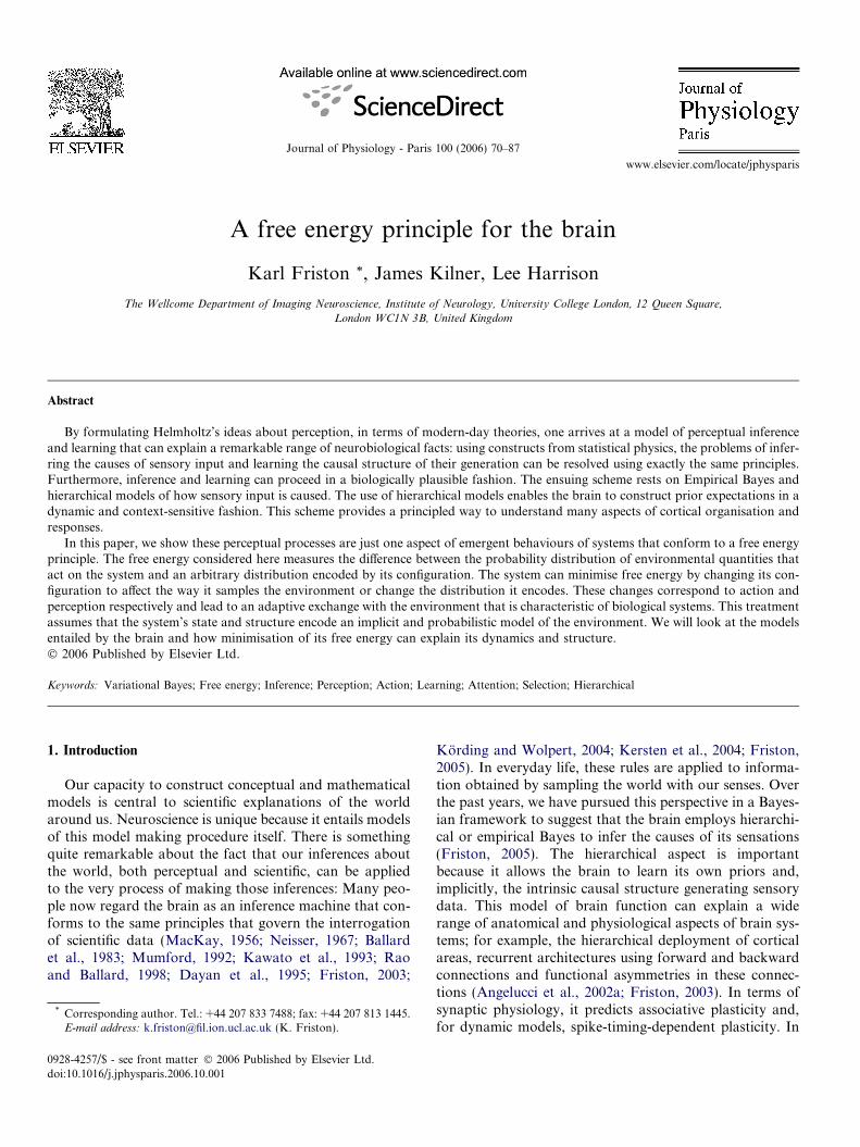
(Ashby, 1947; Nicolis and Prigogine, 1977; Haken, 1983;Kauffman, 1993). However, biological systems are morethan simply dissipative self-organising systems. They cannegotiate a changing or non-stationary environment in away that allows them to endure over substantial periodsof time. This endurance means that they avoid phase tran-sitions that would otherwise change their physical structure(interesting exceptions are phase-transitions in develop-mental trajectories; e.g., in metamorphic insects). A keyaspect of biological systems is that they act upon the envi-ronment to change their position within it, or relation to it,in a way that precludes extremes of temperature, pressureand other external fields. By sampling or navigating theenvironment selectively they restrict their exchange withit within bounds that preserve their physical integrity andallow them to last longer. A fanciful example is providedin Fig. 1: Here, we have taken a paradigm example of anon-biological self-organising system, namely a snowflakeand endowed it with wings that enable it to act on the envi-ronment. A normal snowflake will fall and encounter aphase-boundary, at which the environments temperaturewill cause it to melt. Conversely, snowflakes that can main-tain their altitude, and regulate their temperature, surviveindefinitely with a qualitatively recognisable form. Thekey difference between the normal and adaptive snowflakeis the ability to change their relationship with the environ-

Fig. 1. Schematic highlighting the difference between dissipative, self-organisrelationship to the environment. By occupying a particular environmental nichethat is far from phase-boundaries. The phase-boundary depicted here is a tempea phase-transition). In this fanciful example, we have assumed that snowflatemperature) and avoid being turned into raindrops.

ment and maintain thermodynamic homeostasis. Similarmechanisms can be envisaged easily in an evolutionary set-ting, wherein systems that avoid phase-transitions will beselected above those that cannot (cf., the selection of che-motaxis in single-cell organisms or the phototropic behav-iour of plants). By considering the nature of biologicalsystems in terms of selective pressure one can replace diffi-cult questions about how biological systems emerge withquestions about what behaviours they must exhibit to exist.In other words, selection explains how biological systemsarise; the only outstanding issue is what characterises theymust possess. The snowflake example suggests biologicalsystems act upon the environment to preclude phase-tran-sitions. It is therefore sufficient to define a principle thatensures this sort of exchange with the environment. We willsee that free energy minimisation in one such principle.

4.1. The ensemble density

To develop these arguments formally, we need to definesome quantities that describe the environment, the systemand their interactions. Let # parameterise environmentalforces or fields that act upon the system and k be quantitiesthat describe the systems physical state. We will unpackthese quantities later. At the moment, we will simply notethat they can be very high dimensional and time-varying.

ing systems like snowflakes and adaptive systems that can change their, biological systems can restrict themselves to a domain of parameter spacerature phase-boundary that would cause the snowflake to melt (i.e., inducekes have been given the ability to fly and maintain their altitude (and


To link these two quantities, we will invoke an arbitraryfunction q(#;k), which we will refer to as an ensemble den-sity. This is some arbitrary density function on the environ-ments parameters that is specified or encoded by thesystems parameters. For example, k could be the meanand variance of a Gaussian distribution on the environ-ments temperature, #. The reason q(#;k) is called anensemble density is that it can be regarded as the probabil-ity density that a specific environmental state # would beselected from an infinite ensemble of environments giventhe systems state k. Notice that q(#;k) is not a conditionaldensity because k is treated as fixed and known (as opposedto a random variable).

Invoking the ensemble density links the state of the sys-tem to the environment and allows us to interpret the sys-tem as a probabilistic model of the environment. Theensemble density plays a central role in the free energy for-mulation described below. Before describing this formula-tion, we need to consider two other sets of variables thatdescribe, respectively, the effect of the environment onthe system and the effect of the system on the environment.We will denote these as ~y and a, respectively.1 ~y can bethought of as system states that are acted upon by the envi-ronment; for example the state of sensory receptors. Thismeans that ~y can be regarded as sensory input. The actionvariables a represent the force exerted by effectors that acton the environment to change sensory samples. We willrepresent this dependency by making the sensory samples~yðaÞ a functional of action. Sometimes, this dependencycan be quite simple: For example, the activity of stretchreceptors in muscle spindles is affected directly by muscularforces causing that spindle to contract. In other cases, thedependency can be more complicated: For example, theoculomotor system, controlling eye position, can influencethe activity of every photoreceptor in the retina. Fig. 2shows a schematic of these variables and how they relateto each other. With these quantities in place we can nowformulate an expression for the systems free energy.

5. The free energy principle

The free energy is a scalar function of the ensemble den-sity and the current sensory input. It comprises two terms2

F ¼ �Z

qð#Þ ln pð~y; #Þqð#Þ d#

¼ � ln pð~y; #Þh iq þ ln qð#Þh iq ð1Þ

The first is the energy of this system expected under theensemble density. The energy is simply the surprise orinformation about the joint occurrence of the sensory inputand its causes #. The second term is the negative entropy of

1 Tilde denotes variables in generalised coordinates that cover high-order motion; i.e., ~y ¼ y; y0; y00; . . . This is important when considering thefree energy of dynamic systems and enables a to affect ~y through its high-order temporal derivatives.

2 hÆiq means the expectation under the density q.

the ensemble density. Note that the free energy is definedby two densities; the ensemble density q(#;k) and some-thing we will call the generative density pð~y; #Þ, from whichone can generate sensory samples and their causes. Thegenerative density factorises into a likelihood and priordensity pð~yj#Þpð#Þ, which specify a generative model. Thismeans the free energy induces a generative model for anysystem and an ensemble density over the causes or param-eters of that model. The functional form of these densitiesis needed to evaluate the free energy. We will consider func-tional forms that may be employed by the brain in the nextsection. At the moment, we will just note that these func-tional forms enable the free energy to be defined as a func-tion F ð~y; kÞ of the systems sensory input and state.

The free energy principle states that all the quantitiesthat can change; i.e., that are owned by the system, willchange to minimise free energy. These quantities are thesystem parameters k and the action parameters a. Thisprinciple, as we will see below, is sufficient to account foradaptive exchange with the environment which precludesphase-transitions. We will show this by considering theimplications of minimising the free energy with respect tok and a, respectively.

5.1. Perception: optimising k

It is fairly easy to show that optimizing the systemsparameters with respect to free energy renders the ensembledensity the posterior or conditional density of the environ-mental causes, given the sensory data. This can be seen byrearranging Eq. (1) to show the dependence of the freeenergy on k3

F ¼ � ln pð~yÞ þ Dðqð#; kÞkpð#j~yÞÞ ð2Þ

Only the second term is a function of k; this is a Kullback–Leibler cross-entropy or divergence term that measures thedifference between the ensemble density and the condi-tional density of the causes. Because this measure is alwayspositive, minimising the free energy corresponds to makingthe ensemble density the same as the conditional density. Inother words, the ensemble density encoded by the systemsstate becomes an approximation to the posterior probabil-ity of the causes of its sensory input. This means the systemimplicitly infers or represents the causes of its sensory sam-ples. Clearly, this approximation depends upon the physi-cal structure of the system and the implicit form of theensemble density; and how closely this matches the causalstructure of the environment. Again, invoking selectionistarguments; those systems that match their internal struc-ture to the external causal structure of the environmentin which they are immersed will be able to minimise theirfree energy more effectively.

3 We have used the definition of Kullback–Leibler or relative entropyhere DðqkpÞ ¼

Rq ln q

p d#.

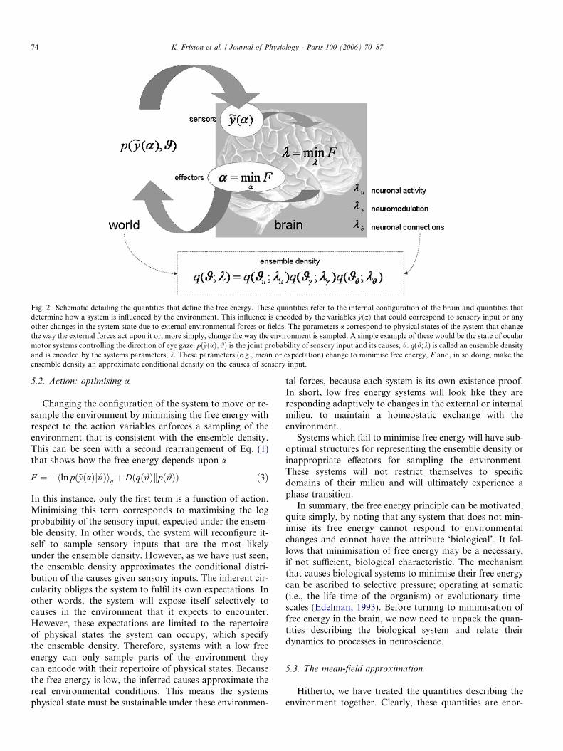
Fig. 2. Schematic detailing the quantities that define the free energy. These quantities refer to the internal configuration of the brain and quantities thatdetermine how a system is influenced by the environment. This influence is encoded by the variables ~yðaÞ that could correspond to sensory input or anyother changes in the system state due to external environmental forces or fields. The parameters a correspond to physical states of the system that changethe way the external forces act upon it or, more simply, change the way the environment is sampled. A simple example of these would be the state of ocularmotor systems controlling the direction of eye gaze. pð~yðaÞ; #Þ is the joint probability of sensory input and its causes, #. q(#;k) is called an ensemble densityand is encoded by the systems parameters, k. These parameters (e.g., mean or expectation) change to minimise free energy, F and, in so doing, make theensemble density an approximate conditional density on the causes of sensory input.


5.2. Action: optimising a

Changing the configuration of the system to move or re-sample the environment by minimising the free energy withrespect to the action variables enforces a sampling of theenvironment that is consistent with the ensemble density.This can be seen with a second rearrangement of Eq. (1)that shows how the free energy depends upon a

F ¼ � ln pð~yðaÞj#Þh iq þ Dðqð#Þkpð#ÞÞ ð3Þ

In this instance, only the first term is a function of action.Minimising this term corresponds to maximising the logprobability of the sensory input, expected under the ensem-ble density. In other words, the system will reconfigure it-self to sample sensory inputs that are the most likelyunder the ensemble density. However, as we have just seen,the ensemble density approximates the conditional distri-bution of the causes given sensory inputs. The inherent cir-cularity obliges the system to fulfil its own expectations. Inother words, the system will expose itself selectively tocauses in the environment that it expects to encounter.However, these expectations are limited to the repertoireof physical states the system can occupy, which specifythe ensemble density. Therefore, systems with a low freeenergy can only sample parts of the environment theycan encode with their repertoire of physical states. Becausethe free energy is low, the inferred causes approximate thereal environmental conditions. This means the systemsphysical state must be sustainable under these environmen-

tal forces, because each system is its own existence proof.In short, low free energy systems will look like they areresponding adaptively to changes in the external or internalmilieu, to maintain a homeostatic exchange with theenvironment.

Systems which fail to minimise free energy will have sub-optimal structures for representing the ensemble density orinappropriate effectors for sampling the environment.These systems will not restrict themselves to specificdomains of their milieu and will ultimately experience aphase transition.

In summary, the free energy principle can be motivated,quite simply, by noting that any system that does not min-imise its free energy cannot respond to environmentalchanges and cannot have the attribute ‘biological’. It fol-lows that minimisation of free energy may be a necessary,if not sufficient, biological characteristic. The mechanismthat causes biological systems to minimise their free energycan be ascribed to selective pressure; operating at somatic(i.e., the life time of the organism) or evolutionary time-scales (Edelman, 1993). Before turning to minimisation offree energy in the brain, we now need to unpack the quan-tities describing the biological system and relate theirdynamics to processes in neuroscience.

5.3. The mean-field approximation

Hitherto, we have treated the quantities describing theenvironment together. Clearly, these quantities are enor-


mous in number and variety. A key difference among themis the timescales over which they change. We will use thisdistinction to partition the parameters into three sets# = #u,#c,#h that change quickly, slowly and very slowly;and factorise the ensemble density

qð#Þ ¼Y

i

qð#i; kiÞ ¼ qð#u; kuÞqð#c; kcÞqð#h; khÞ ð4Þ

This also induces a partitioning of the systems parametersinto k = ku,kc,kh that encode time-varying partitions of theensemble density. The first set ku, are system quantities thatchange rapidly. These could correspond to neuronal activ-ity or electromagnetic states of the brain and change with atimescale of milliseconds. The causes #u they encode, corre-spond to rapidly changing environmental states, for exam-ple, changes in the environment caused by structuralinstabilities or other organisms.

The second set kc change more slowly, over a time scaleof seconds. These could correspond to the kinetics of molec-ular signalling in neurons; for example calcium-dependentmechanisms underlying short-term changes in synaptic effi-cacy and classical neural modulatory effects. The equivalentpartition of causes in the environment may be contextual innature, such as the level of radiant illumination or the influ-ence of slowly varying external fields that set the context formore rapid fluctuations in its state.

Finally, kh represent system quantities that changeslowly; for example long-term changes in synaptic connec-tions during experience-dependent plasticity, or the deploy-ment of axons that change on a neurodevelopmentaltimescale. The homologous quantities in the environmentare invariances in the causal architecture. These could cor-respond to physical laws and other structural regularitiesthat shape our interaction with the world.

The factorization in Eq. (4) is, in statistical physics,known as a mean-field approximation. Clearly our approxi-mation with three partitions is a little arbitrary, but it helpsorganise the functional correlates of their respective optimi-sation in the nervous system. Other timescales would be nec-essary for other systems like plants. The mean-fieldapproximation greatly finesses the minimisation of freeenergy when considering particular schemes. These schemesusually employ variational techniques. Variationalapproaches were introduced by Feynman (1972), in the con-text of quantum mechanics using the path integral formula-tion. They have been adopted widely by the machine learningcommunity (e.g., Hinton and von Cramp, 1993; MacKay,1995). Established statistical methods like expectation max-imisation and restricted maximum likelihood (Dempsteret al., 1977; Harville, 1977) can be formulated in terms of freeenergy (Neal and Hinton, 1998; Friston et al., in press).

6. Optimising variational modes

We now revisit optimisation of the systems parametersthat underlie perception in more detail, using the mean-field approximation. Because variational techniques pre-

dominate under this approximation, the free energy inEq. (1) is also known as the variational free energy andki are called variational parameters. The mean-field factori-sation means that the mean-field approximation cannotcover the effect of random fluctuations in one partition,on the fluctuations in another. However, this is not a severelimitation because these effects are modelled through mean-field effects (i.e., through the means or dispersions of ran-dom fluctuations). This approximation is particularly easyto motivate in the present framework because random fluc-tuations at fast timescales are unlikely to have a directeffect at slower timescales.

Using variational calculus it is simple to show (see Fris-ton et al., in press) that, under the mean-field approxima-tion above, the ensemble density has the following form:

qð#iÞ / expðIð#iÞÞIð#iÞ ¼ ln pð~y; #Þh iqni

ð5Þ

where I(#i) is simply the log-probability of #i and the dataexpected under the ensemble density of the other parti-tions, qni. We will call this the variational energy. FromEq. (5) it is evident that the mode of the ensemble densitymaximises the variational energy. The mode is an impor-tant variational parameter. For example, if we assumeq(#i) is Gaussian, then it is parameterised by two varia-tional parameters ki = li,Ri encoding the mode and covari-ance, respectively. This is known as the Laplaceapproximation and will be used later. In what follows, wewill focus on minimising the free energy by optimizing li;noting that there may be other variational parametersdescribing higher moments of the ensemble density, foreach partition. Fortunately, under the Laplace approxima-tion, the only other variational parameter we require is thecovariance. This has a simple form, which is an analyticfunction of the mode and therefore does not need to be rep-resented explicitly (see Friston et al., in press and AppendixA). We now look at the optimisation of the variationalmodes li and the neurobiological and cognitive processesthis optimisation entails:

6.1. Perceptual inference: optimising lu

Minimising the free energy with respect to neuronalstates lu means maximising I(#u)

lu ¼ max Ið#uÞIð#uÞ ¼ ln pð~yj#Þ þ ln pð#Þh iqcqh

¼ ln pð#j~yÞh iqcqhþ ln pð~yÞ

ð6Þ

This means that the free energy principle is served when thevariational mode of the states (i.e., neuronal activity)changes to maximize its log-posterior, expected under theensemble density of causes that change more slowly. Thiscan be achieved, without knowing the true posterior, bymaximising the expected log-likelihood and prior that spec-ify a probabilistic generative model (second line of Eq. (6)).

4 In the simulations below, we take the expectation over peristimulustime.


As mentioned above, this optimisation requires the func-tional form of the generative model. In the next section,we will look at hierarchical forms that are commensuratewith the structure of the brain. For now, it is sufficient tonote that the free energy principle means that brain stateswill come to encode the most likely state of the environ-ment that is causing sensory input.

6.2. Generalised coordinates

Because states are time-varying quantities, it is impor-tant to consider what their ensemble density covers. Thiscan cover not just the states at one moment in time buttheir higher-order motion. In other words, a particularstate of the environment and its probabilistic encoding inthe brain can embody dynamics by representing the trajec-tories of states in generalised coordinates. Generalisedcoordinates are a common device in physics and normallycover position and momentum. In the present context, ageneralised state includes the current state, and its general-ised motion #u = u,u 0,u00, . . . with corresponding varia-tional modes lu; l

0u; l

00u; . . . It is fairly simple to show

(Friston, in preparation) that the extremisation in Eq. (6)can be achieved with a rapid gradient descent, while cou-pling higher to lower-order motion via mean-field terms

_lu ¼ joIð#uÞ=ouþ l0u_l0u ¼ joIð#uÞ=ou0 þ l00u_l00u ¼ joIð#uÞ=ou00 þ l000u_l000u ¼ � � �

ð7Þ

Here _lu mean the rate of change of lu and j is some suit-able rate constant. The simulations in the next section usethis descent scheme, which can be implemented using rela-tively simple neural networks. Note, when the conditionalmode has found the maximum of I(#u), its gradient is zeroand the motion of the mode becomes the mode of the mo-tion; i.e., _lu ¼ l0u. However, it is perfectly possible, in gen-eralised coordinates, for these quantities to differ, unlessthere are special constraints. At the level of perception,psychophysical phenomena, like the motion after-effect,suggest the brain uses generalised coordinates; for example,on stopping, after a period of looking at the scenery from amoving train, the world is perceived as moving but withoutchanging its position. The impression that visual objectschange their position in accord with their motion is some-thing that our brains have learned about the causal struc-ture of the world. It is also something that can beunlearned, temporarily (e.g., perceptual after-effects). Wenow turn to how these causal regularities are learned.

6.3. Perceptual context and attention: optimising lc

If we call the causes that change on an intermediatetimescale, #c contextual, then optimizing lc correspondsto encoding the probabilistic contingencies in which thefast dynamics of the states evolve. This optimization can

proceed as above; however, we can assume that the contextchanges sufficiently slowly that we can make the approxi-mation l0c ¼ 0. This gives the simple gradient ascent

_lc ¼ joIð#cÞ=o#c

Ið#cÞ ¼ ln pð~y; #Þh iquqh

ð8Þ

Note that the expectation is over the generalised coordinatesof the states and, implicitly, an extended period of time overwhich the state trajectory evolves.4 We will see below that theconditional mode lc encoding context might correspond tothe strength of lateral or horizontal interactions betweenneurons in the brain. These lateral interactions control therelative effects of top-down and bottom-up influences onthe expected states and therefore control the balance be-tween empirical priors and sensory information, in makingperceptual inferences. This suggests that attention could bethought of in terms of optimizing contextual parameters ofthis sort. It is important to note that, in Eq. (8), the dynamicsof lc are determined by the expectation under the ensembledensity of the perceptual states. This means that it is possiblefor the system to adjust its internal representation of proba-bilistic contingencies in a way that is sensitive to the statesand their history. A simple example of this, in psychology,would be the Posner paradigm, where a perceptual state;namely an orienting cue, directs visual attention to a partic-ular part of visual space in which a target cue will be pre-sented. In terms of the current formulation, this wouldcorrespond to a state-dependent change in the variationalparameters encoding context that bias perceptual inferencetowards the cued part of the sensorium (we will model thisin subsequent communication).

The key point here is that the mean-field approximationallows for inferences about rapidly changing perceptualstates and more slowly changing context to influence eachother through mean-field effects (i.e., the expectations inEqs. (6) and (8)). This can proceed without explicitly repre-senting the joint distribution in an ensemble density overstate and context explicitly (cf., Rao, 2005). Anotherimportant interaction between variational parametersrelates to the encoding of uncertainly. Under the Laplaceassumption this is encoded by the conditional covariances.Critically the conditional covariance of one ensemble is afunction of the conditional mode of the others (see Eq.(A.2) in Appendix A). In the present context, the influenceof context on perceptual inference can be cast in terms ofencoding uncertainty. We will look at neuronal implemen-tations of this in the next section.

6.4. Perceptual learning: optimising lh

Optimizing the variational mode encoding #h corre-sponds to inferring and learning structural regularities in

5 In machine learning, one usually regards the free energy as an upperbound on the log-evidence.


the causal architecture of the environment. As above, thislearning can be implemented as a gradient ascent onI(#h), which represents an expectation under the ensembledensity encoding the generalised states and context

_lh ¼ joIð#hÞ=o#h

Ið#hÞ ¼ ln pð~y; #Þh iquqc

ð9Þ

In the brain, this descent can be formulated as changes inconnections that are a function of pre-synaptic predictionand post-synaptic prediction error (see Friston, 2003,2005). The ensuing learning rule conforms to simple asso-ciative plasticity or, in dynamic models, plasticity thatlooks like spike-timing-dependent plasticity. In the sensethat optimizing the variational parameters that correspondto connection strengths in the brain encodes causal struc-ture in the environment; this instance of free energy mini-misation corresponds to learning. The implicit change inthe brains connectivity endows it with a memory of pastinteractions with the environment that affects the free en-ergy dynamics underlying perception and attention. Thisis through the mean-field effects in Eqs. (6) and (8). Putsimply, sustained exposure to environmental inputs causesthe internal structure of the brain to recapitulate the causalstructure of those inputs. In turn, this enables efficient per-ceptual inference. This formulation provides a transparentaccount of perceptual learning and categorization, whichenables the system to remember associations and contin-gencies among causal states and context. The extensionof these ideas into episodic memory remains an outstand-ing challenge.

7. Model optimisation

Hitherto, we have only considered the quantitative opti-misation of variational parameters given a particular sys-tem and its implicit generative model. Exactly the samefree energy principle can be applied to optimise the modelitself. Different models can come from populations of sys-tems or from qualitative changes in one system over time.A model here corresponds to a particular configurationthat can be enumerated with the same set of variationalparameters. Removing a part of the system or adding,for example, another set of connections, changes the modeland the variational parameters in a qualitative or categor-ical fashion.

Model optimisation involves maximising the marginallikelihood of the model itself. In statistics and machinelearning this is equivalent to Bayesian model selection,where the free energy can be used to approximate the mar-ginal likelihood, pð~yjmiÞ or evidence for a particular modelmi. This approximation can be motivated easily using Eq.(2): If the system has minimised its free energy and thedivergence term is near zero, then the free energyapproaches the negative log-evidence for that model.Therefore, the model with the smallest free energy hasthe highest marginal likelihood.

An evolutionary perceptive on this considers the log-evi-dence as a lower-bound on free energy,5 which is definedfor any systems exchange with the environment ~yðaÞ andis independent of the systems parameters k. An adaptivesystem will keep this exchange within bounds that ensureits physical integrity. All this requires is the selection ofan appropriate model that renders the log-evidence con-cave within these bounds and processes that minimise itsfree energy (see Fig. 2). Selecting models with the lowestfree energy will select models that are best able to modeltheir environmental niche and therefore remain within it.Notice that this hierarchical selection rests upon interplaybetween optimising the parameters of a particular model(to minimise the free energy) and optimising the modelper se (using the minimised free energy). Optimisation atboth levels is prescribed by the free energy principle. Inthe theory of genetic algorithms, this is called hierarchicalcoevolution (e.g., Maniadakis and Trahanias, 2006). Asimilar relationship is found in Bayesian inference, wheremodel selection is based on a free energy approximationto the model evidence that is furnished by optimising theparameters of each model to minimise free energy. In short,free energy may be a useful surrogate for adaptive fitness inan evolutionary setting and the marginal likelihood inmodel selection. We introduce model selection because itis linked to value learning (Fig. 3).

7.1. Value-learning: optimising mi

Value-learning here denotes the ability of a system tolearn valuable or adaptive responses. It refers to re-enforce-ment or emotional learning in the psychological literatureand is closely related to dynamic programming (e.g., tem-poral difference models) in the engineering and neurosci-ence literature (e.g., Montague et al., 1995; Suri andSchultz, 2001). In an early formulation of value-learning(Friston et al., 1994) we introduced the distinction betweeninnate and acquired value. Innate value is an attribute ofstimuli or sensory input that releases genetically or epige-netically specified responses that confer fitness. Acquiredvalue is an attribute of stimuli that comes to evoke behav-iours, which ultimately disclose stimuli or cues with innatevalue. Acquired value is therefore learnt during neurode-velopment and exposure to the environment.

The free energy principle explains adaptive behaviourwithout invoking notions of acquired value or re-enforce-ment: From the point of view of the organism, it is simplysampling the environment so that its sensory input con-forms to its expectations. From its perspective, the envi-ronment is a stable and accommodating place. However,for someone observing this system, it will appear torespond adaptively to environmental changes and avoidadverse conditions. In other words, it will seem as if certain

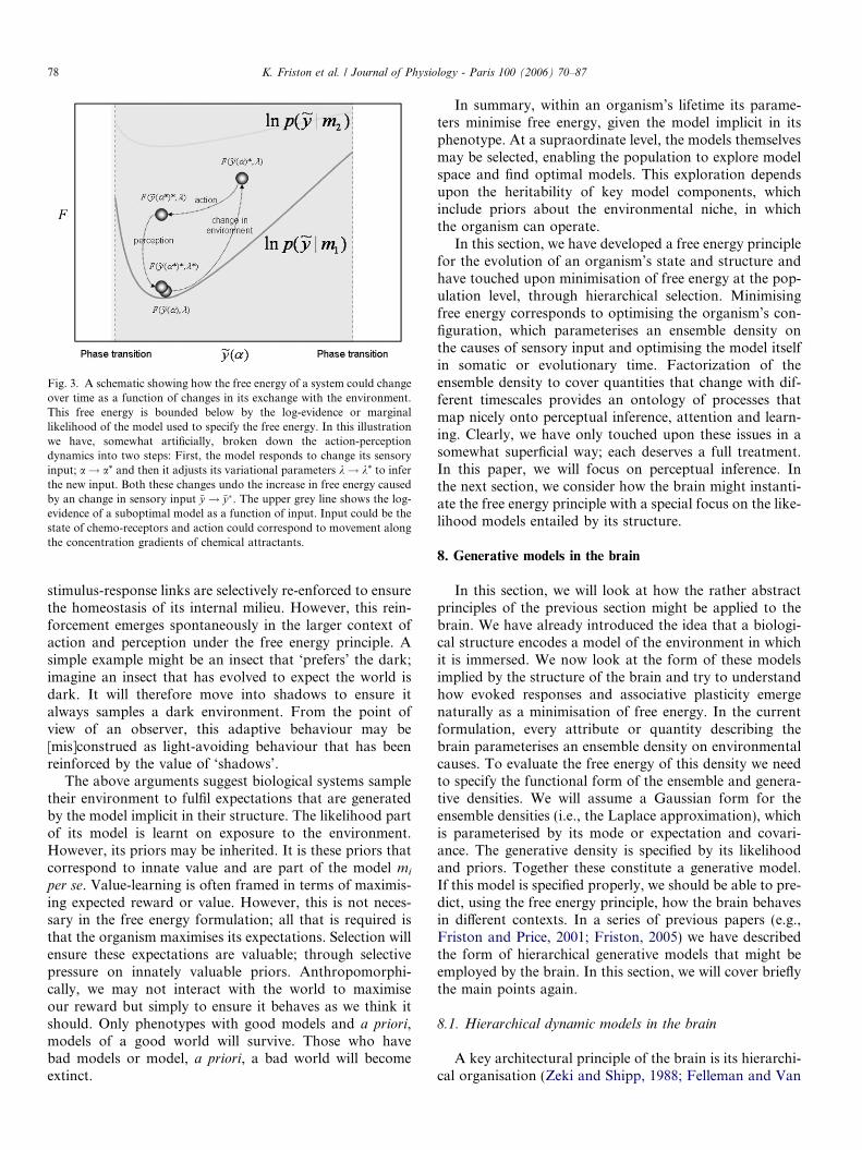
Fig. 3. A schematic showing how the free energy of a system could changeover time as a function of changes in its exchange with the environment.This free energy is bounded below by the log-evidence or marginallikelihood of the model used to specify the free energy. In this illustrationwe have, somewhat artificially, broken down the action-perceptiondynamics into two steps: First, the model responds to change its sensoryinput; a! a* and then it adjusts its variational parameters k! k* to inferthe new input. Both these changes undo the increase in free energy causedby an change in sensory input ~y ! ~y�. The upper grey line shows the log-evidence of a suboptimal model as a function of input. Input could be thestate of chemo-receptors and action could correspond to movement alongthe concentration gradients of chemical attractants.


stimulus-response links are selectively re-enforced to ensurethe homeostasis of its internal milieu. However, this rein-forcement emerges spontaneously in the larger context ofaction and perception under the free energy principle. Asimple example might be an insect that ‘prefers’ the dark;imagine an insect that has evolved to expect the world isdark. It will therefore move into shadows to ensure italways samples a dark environment. From the point ofview of an observer, this adaptive behaviour may be[mis]construed as light-avoiding behaviour that has beenreinforced by the value of ‘shadows’.

The above arguments suggest biological systems sampletheir environment to fulfil expectations that are generatedby the model implicit in their structure. The likelihood partof its model is learnt on exposure to the environment.However, its priors may be inherited. It is these priors thatcorrespond to innate value and are part of the model mi

per se. Value-learning is often framed in terms of maximis-ing expected reward or value. However, this is not neces-sary in the free energy formulation; all that is required isthat the organism maximises its expectations. Selection willensure these expectations are valuable; through selectivepressure on innately valuable priors. Anthropomorphi-cally, we may not interact with the world to maximiseour reward but simply to ensure it behaves as we think itshould. Only phenotypes with good models and a priori,models of a good world will survive. Those who havebad models or model, a priori, a bad world will becomeextinct.

In summary, within an organism’s lifetime its parame-ters minimise free energy, given the model implicit in itsphenotype. At a supraordinate level, the models themselvesmay be selected, enabling the population to explore modelspace and find optimal models. This exploration dependsupon the heritability of key model components, whichinclude priors about the environmental niche, in whichthe organism can operate.

In this section, we have developed a free energy principlefor the evolution of an organism’s state and structure andhave touched upon minimisation of free energy at the pop-ulation level, through hierarchical selection. Minimisingfree energy corresponds to optimising the organism’s con-figuration, which parameterises an ensemble density onthe causes of sensory input and optimising the model itselfin somatic or evolutionary time. Factorization of theensemble density to cover quantities that change with dif-ferent timescales provides an ontology of processes thatmap nicely onto perceptual inference, attention and learn-ing. Clearly, we have only touched upon these issues in asomewhat superficial way; each deserves a full treatment.In this paper, we will focus on perceptual inference. Inthe next section, we consider how the brain might instanti-ate the free energy principle with a special focus on the like-lihood models entailed by its structure.

8. Generative models in the brain

In this section, we will look at how the rather abstractprinciples of the previous section might be applied to thebrain. We have already introduced the idea that a biologi-cal structure encodes a model of the environment in whichit is immersed. We now look at the form of these modelsimplied by the structure of the brain and try to understandhow evoked responses and associative plasticity emergenaturally as a minimisation of free energy. In the currentformulation, every attribute or quantity describing thebrain parameterises an ensemble density on environmentalcauses. To evaluate the free energy of this density we needto specify the functional form of the ensemble and genera-tive densities. We will assume a Gaussian form for theensemble densities (i.e., the Laplace approximation), whichis parameterised by its mode or expectation and covari-ance. The generative density is specified by its likelihoodand priors. Together these constitute a generative model.If this model is specified properly, we should be able to pre-dict, using the free energy principle, how the brain behavesin different contexts. In a series of previous papers (e.g.,Friston and Price, 2001; Friston, 2005) we have describedthe form of hierarchical generative models that might beemployed by the brain. In this section, we will cover brieflythe main points again.

8.1. Hierarchical dynamic models in the brain

A key architectural principle of the brain is its hierarchi-cal organisation (Zeki and Shipp, 1988; Felleman and Van


Essen, 1991; Mesulam, 1998; Hochstein and Ahissar, 2002)This organisation has been studied most thoroughly in thevisual system, where cortical areas can be regarded asforming a hierarchy; with lower areas being closer to pri-mary sensory input and higher areas adopting a multi-modal or associational role. The notion of a hierarchyrests upon the distinction between forward and backwardconnections (Rockland and Pandya, 1979; Murphy andSillito, 1987; Felleman and Van Essen, 1991; Shermanand Guillery, 1998; Angelucci et al., 2002a). The distinctionbetween forward and backward connections is based on thespecificity of the cortical layers that are the predominantsources and origins of extrinsic connections in the brain.Forward connections arise largely in superficial pyramidalcells, in supra-granular layers and terminate in spiny stel-late cells of layer four or the granular layer of a higher cor-tical area (Felleman and Van Essen, 1991; DeFelipe et al.,2002). Conversely, backward connections arise largelyfrom deep pyramidal cells in infra-granular layers and tar-get cells in the infra and supra granular layers of lower cor-tical areas. Intrinsic connections are both intra and interlaminar and mediate lateral interactions between neuronsthat are a few millimetres away. Due to convergence anddivergence of extrinsic forward and backward connections,receptive fields of higher areas are generally larger thanlower areas (Zeki and Shipp, 1988). There is a keyfunctional distinction between forward and backward con-nections that renders backward connections more modula-tory or non-linear in their effects on neuronal responses(e.g., Sherman and Guillery, 1998). This is consistent withthe deployment of voltage sensitive and non-linear NMDAreceptors in the supra-granular layers that are targeted bybackward connections. Typically, the synaptic dynamicsof backward connections have slower time constants. Thishas led to the notion that forward connections are drivingand illicit an obligatory response in higher levels, whereasbackward connections have both driving and modulatoryeffects and operate over greater spatial and temporal scales.

The hierarchical structure of the brain speaks to hierar-chical models of sensory input. For example

y ¼ gðxð1Þ; vð1ÞÞ þ zð1Þ

_xð1Þ ¼ f ðxð1Þ; vð1ÞÞ þ wð1Þ

..

.

vði�1Þ ¼ gðxðiÞ; vðiÞÞ þ zðiÞ

_xðiÞ ¼ f ðxðiÞ; vðiÞÞ þ wðiÞ

..

.

ð10Þ

In this model sensory states y are caused by a non-linearfunction of states, g(x(1),v(1)) plus a random effect z(1).The dynamic states x(1) have memory and evolve accordingto equations of motion prescribed by the non-linear func-tion f(x(1),v(1)). These dynamics are subject to random fluc-tuations w(1) and perturbations from higher levels that aregenerated in exactly the same way. In other words, the in-

put to any level is the output of the level above. This meanscasual states v(i) link hierarchical levels and dynamic statesx(i) generate dynamics that are intrinsic to each level. Therandom fluctuations can be assumed to be Gaussian witha covariance encoded by the hyper-parameters #ðiÞc . Thefunctions at each level are parameterised by #

ðiÞh . This form

of hierarchical dynamical model is extremely generic andsubsumes most models found in statistics and machinelearning as special cases.

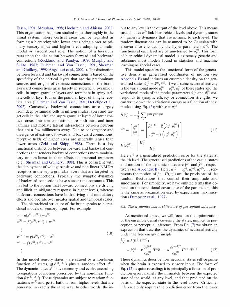
This model specifies the functional form of the genera-tive density in generalised coordinates of motion (seeAppendix B) and induces an ensemble density on the gen-eralised states #ðiÞu ¼ ~xðiÞ;~vðiÞ. If we assume neuronal activityis the variational mode ~lðiÞu ¼ ~lðiÞv ; ~l

ðiÞx of these states and the

variational mode of the model parameters #ðiÞc and #ðiÞh cor-responds to synaptic efficacy or connection strengths; wecan write down the variational energy as a function of thesemodes using Eq. (5); with y ¼ lð0Þv

Ið~luÞ ¼ �1

2

Xi

~eðiÞT PðiÞ~eðiÞ

~eðiÞ ¼~eðiÞv

~eðiÞx

" #¼

~lði�1Þv � ~g ~lðiÞu ; l

ðiÞh

� �~l0ðiÞx � ~f ~lðiÞu ; l

ðiÞh

� �264

375 ð11Þ

PðlðiÞc Þ ¼PðiÞz

PðiÞw

" #

Here ~eðiÞ is a generalised prediction error for the states atthe ith level. The generalised predictions of the casual statesand motion of the dynamic states are ~gðiÞ and ~f ðiÞ, respec-tively (see Appendix B). Here, ~l0ðiÞ ¼ l0ðiÞx ; l00ðiÞx ; l000ðiÞx ; . . . rep-resents the motion of ~lðiÞx . PðlðiÞc Þ are the precisions of therandom fluctuations that control their amplitude andsmoothness. For simplicity, we have omitted terms that de-pend on the conditional covariance of the parameters; thisis the same approximation used by expectation maximisa-tion (Dempster et al., 1977).

8.2. The dynamics and architecture of perceptual inference

As mentioned above, we will focus on the optimizationof the ensemble density covering the states, implicit in per-ception or perceptual inference. From Eq. (7) we obtain anexpression that describes the dynamics of neuronal activityunder the free energy principle

_~lðiÞu ¼ hð~eðiÞ;~eðiþ1ÞÞ

¼ ~l0ðiÞu � jo~eðiÞT

o~lðiÞu

PðiÞ~eðiÞ � jo~eðiþ1ÞT

o~lðiÞu

Pðiþ1Þ~eðiþ1Þ ð12Þ

These dynamics describe how neuronal states self-organisewhen the brain is exposed to sensory input. The form ofEq. (12) is quite revealing; it is principally a function of pre-diction error, namely the mismatch between the expectedstate of the world, at any level, and that predicted on thebasis of the expected state in the level above. Critically,inference only requires the prediction error from the lower

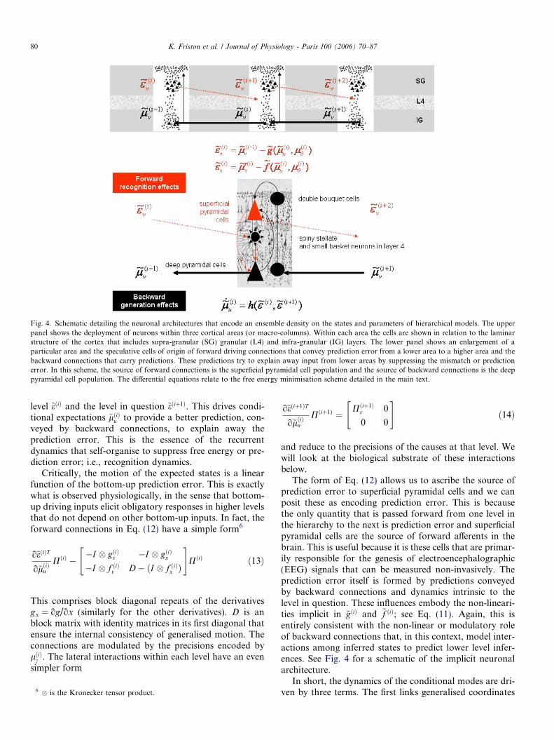
Fig. 4. Schematic detailing the neuronal architectures that encode an ensemble density on the states and parameters of hierarchical models. The upperpanel shows the deployment of neurons within three cortical areas (or macro-columns). Within each area the cells are shown in relation to the laminarstructure of the cortex that includes supra-granular (SG) granular (L4) and infra-granular (IG) layers. The lower panel shows an enlargement of aparticular area and the speculative cells of origin of forward driving connections that convey prediction error from a lower area to a higher area and thebackward connections that carry predictions. These predictions try to explain away input from lower areas by suppressing the mismatch or predictionerror. In this scheme, the source of forward connections is the superficial pyramidal cell population and the source of backward connections is the deeppyramidal cell population. The differential equations relate to the free energy minimisation scheme detailed in the main text.


level ~eðiÞ and the level in question ~eðiþ1Þ. This drives condi-tional expectations ~lðiÞu to provide a better prediction, con-veyed by backward connections, to explain away theprediction error. This is the essence of the recurrentdynamics that self-organise to suppress free energy or pre-diction error; i.e., recognition dynamics.

Critically, the motion of the expected states is a linearfunction of the bottom-up prediction error. This is exactlywhat is observed physiologically, in the sense that bottom-up driving inputs elicit obligatory responses in higher levelsthat do not depend on other bottom-up inputs. In fact, theforward connections in Eq. (12) have a simple form6

o~eðiÞT

o~lðiÞu

PðiÞ � �I � gðiÞv �I � gðiÞx

�I � f ðiÞv D� ðI � f ðiÞx Þ

" #PðiÞ ð13Þ

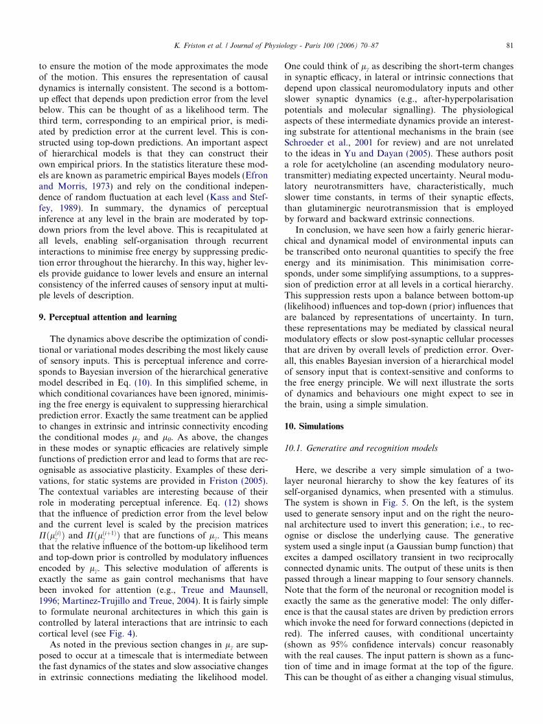
This comprises block diagonal repeats of the derivativesgx = og/ox (similarly for the other derivatives). D is anblock matrix with identity matrices in its first diagonal thatensure the internal consistency of generalised motion. Theconnections are modulated by the precisions encoded bylðiÞc . The lateral interactions within each level have an evensimpler form

6 � is the Kronecker tensor product.

o~eðiþ1ÞT

o~lðiÞu

Pðiþ1Þ ¼ Pðiþ1Þv 0

0 0

" #ð14Þ

and reduce to the precisions of the causes at that level. Wewill look at the biological substrate of these interactionsbelow.

The form of Eq. (12) allows us to ascribe the source ofprediction error to superficial pyramidal cells and we canposit these as encoding prediction error. This is becausethe only quantity that is passed forward from one level inthe hierarchy to the next is prediction error and superficialpyramidal cells are the source of forward afferents in thebrain. This is useful because it is these cells that are primar-ily responsible for the genesis of electroencephalographic(EEG) signals that can be measured non-invasively. Theprediction error itself is formed by predictions conveyedby backward connections and dynamics intrinsic to thelevel in question. These influences embody the non-lineari-ties implicit in ~gðiÞ and ~f ðiÞ; see Eq. (11). Again, this isentirely consistent with the non-linear or modulatory roleof backward connections that, in this context, model inter-actions among inferred states to predict lower level infer-ences. See Fig. 4 for a schematic of the implicit neuronalarchitecture.

In short, the dynamics of the conditional modes are dri-ven by three terms. The first links generalised coordinates


to ensure the motion of the mode approximates the modeof the motion. This ensures the representation of causaldynamics is internally consistent. The second is a bottom-up effect that depends upon prediction error from the levelbelow. This can be thought of as a likelihood term. Thethird term, corresponding to an empirical prior, is medi-ated by prediction error at the current level. This is con-structed using top-down predictions. An important aspectof hierarchical models is that they can construct theirown empirical priors. In the statistics literature these mod-els are known as parametric empirical Bayes models (Efronand Morris, 1973) and rely on the conditional indepen-dence of random fluctuation at each level (Kass and Stef-fey, 1989). In summary, the dynamics of perceptualinference at any level in the brain are moderated by top-down priors from the level above. This is recapitulated atall levels, enabling self-organisation through recurrentinteractions to minimise free energy by suppressing predic-tion error throughout the hierarchy. In this way, higher lev-els provide guidance to lower levels and ensure an internalconsistency of the inferred causes of sensory input at multi-ple levels of description.

9. Perceptual attention and learning

The dynamics above describe the optimization of condi-tional or variational modes describing the most likely causeof sensory inputs. This is perceptual inference and corre-sponds to Bayesian inversion of the hierarchical generativemodel described in Eq. (10). In this simplified scheme, inwhich conditional covariances have been ignored, minimis-ing the free energy is equivalent to suppressing hierarchicalprediction error. Exactly the same treatment can be appliedto changes in extrinsic and intrinsic connectivity encodingthe conditional modes lc and lh. As above, the changesin these modes or synaptic efficacies are relatively simplefunctions of prediction error and lead to forms that are rec-ognisable as associative plasticity. Examples of these deri-vations, for static systems are provided in Friston (2005).The contextual variables are interesting because of theirrole in moderating perceptual inference. Eq. (12) showsthat the influence of prediction error from the level belowand the current level is scaled by the precision matricesPðlðiÞc Þ and Pðlðiþ1Þ

c Þ that are functions of lc. This meansthat the relative influence of the bottom-up likelihood termand top-down prior is controlled by modulatory influencesencoded by lc. This selective modulation of afferents isexactly the same as gain control mechanisms that havebeen invoked for attention (e.g., Treue and Maunsell,1996; Martinez-Trujillo and Treue, 2004). It is fairly simpleto formulate neuronal architectures in which this gain iscontrolled by lateral interactions that are intrinsic to eachcortical level (see Fig. 4).

As noted in the previous section changes in lc are sup-posed to occur at a timescale that is intermediate betweenthe fast dynamics of the states and slow associative changesin extrinsic connections mediating the likelihood model.

One could think of lc as describing the short-term changesin synaptic efficacy, in lateral or intrinsic connections thatdepend upon classical neuromodulatory inputs and otherslower synaptic dynamics (e.g., after-hyperpolarisationpotentials and molecular signalling). The physiologicalaspects of these intermediate dynamics provide an interest-ing substrate for attentional mechanisms in the brain (seeSchroeder et al., 2001 for review) and are not unrelatedto the ideas in Yu and Dayan (2005). These authors posita role for acetylcholine (an ascending modulatory neuro-transmitter) mediating expected uncertainty. Neural modu-latory neurotransmitters have, characteristically, muchslower time constants, in terms of their synaptic effects,than glutaminergic neurotransmission that is employedby forward and backward extrinsic connections.

In conclusion, we have seen how a fairly generic hierar-chical and dynamical model of environmental inputs canbe transcribed onto neuronal quantities to specify the freeenergy and its minimisation. This minimisation corre-sponds, under some simplifying assumptions, to a suppres-sion of prediction error at all levels in a cortical hierarchy.This suppression rests upon a balance between bottom-up(likelihood) influences and top-down (prior) influences thatare balanced by representations of uncertainty. In turn,these representations may be mediated by classical neuralmodulatory effects or slow post-synaptic cellular processesthat are driven by overall levels of prediction error. Over-all, this enables Bayesian inversion of a hierarchical modelof sensory input that is context-sensitive and conforms tothe free energy principle. We will next illustrate the sortsof dynamics and behaviours one might expect to see inthe brain, using a simple simulation.

10. Simulations

10.1. Generative and recognition models

Here, we describe a very simple simulation of a two-layer neuronal hierarchy to show the key features of itsself-organised dynamics, when presented with a stimulus.The system is shown in Fig. 5. On the left, is the systemused to generate sensory input and on the right the neuro-nal architecture used to invert this generation; i.e., to rec-ognise or disclose the underlying cause. The generativesystem used a single input (a Gaussian bump function) thatexcites a damped oscillatory transient in two reciprocallyconnected dynamic units. The output of these units is thenpassed through a linear mapping to four sensory channels.Note that the form of the neuronal or recognition model isexactly the same as the generative model: The only differ-ence is that the causal states are driven by prediction errorswhich invoke the need for forward connections (depicted inred). The inferred causes, with conditional uncertainty(shown as 95% confidence intervals) concur reasonablywith the real causes. The input pattern is shown as a func-tion of time and in image format at the top of the figure.This can be thought of as either a changing visual stimulus,

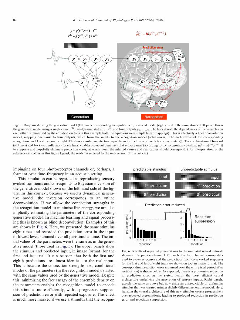
Fig. 5. Diagram showing the generative model (left) and corresponding recognition; i.e., neuronal model (right) used in the simulations. Left panel: this isthe generative model using a single cause v(1), two dynamic states xð1Þ1 ; xð1Þ2 and four outputs y1, . . . ,y4. The lines denote the dependencies of the variables oneach other, summarised by the equation on top (in this example both the equations were simple linear mappings). This is effectively a linear convolutionmodel, mapping one cause to four outputs, which form the inputs to the recognition model (solid arrow). The architecture of the correspondingrecognition model is shown on the right. This has a similar architecture, apart from the inclusion of prediction error units; ~eðiÞu . The combination of forward(red lines) and backward influences (black lines) enables recurrent dynamics that self-organise (according to the recognition equation; _~lðiÞu ¼ hð~eðiÞ;~eðiþ1ÞÞÞto suppress and hopefully eliminate prediction error, at which point the inferred causes and real causes should correspond. (For interpretation of thereferences in colour in this figure legend, the reader is referred to the web version of this article.)

Fig. 6. Results of repeated presentations to the simulated neural networkshown in the previous figure. Left panels: the four channel sensory dataused to evoke responses and the predictions from these evoked responsesfor the first and last of eight trials are shown on top, in image format. Thecorresponding prediction error (summed over the entire trial period afterrectification) is shown below. As expected, there is a progressive reductionin prediction error as the system learns the most efficient causalarchitecture underlying the generation of sensory inputs. Right panels:exactly the same as above but now using an unpredictable or unfamiliarstimulus that was created using a slightly different generative model. Here,learning the causal architecture of this new stimulus occurs progressivelyover repeated presentations, leading to profound reduction in predictionerror and repetition suppression.


impinging on four photo-receptor channels or, perhaps, aformant over time–frequency in an acoustic setting.

This simulation can be regarded as reproducing sensoryevoked transients and corresponds to Bayesian inversion ofthe generative model shown on the left hand side of the fig-ure. In this context, because we used a dynamical genera-tive model, the inversion corresponds to an onlinedeconvolution. If we allow the connection strengths inthe recognition model to minimise free energy, we are alsoimplicitly estimating the parameters of the correspondinggenerative model. In machine learning and signal process-ing this is known as blind deconvolution. Examples of thisare shown in Fig. 6. Here, we presented the same stimuluseight times and recorded the prediction error in the inputor lowest level, summed over all peristimulus time. The ini-tial values of the parameters were the same as in the gener-ative model (those used in Fig. 5). The upper panels showthe stimulus and predicted input, in image format, for thefirst and last trial. It can be seen that both the first andeighth predictions are almost identical to the real input.This is because the connection strengths, i.e., conditionalmodes of the parameters (in the recognition model), startedwith the same values used by the generative model. Despitethis, minimising the free energy of the ensemble density onthe parameters enables the recognition model to encodethis stimulus more efficiently, with a progressive suppres-sion of prediction error with repeated exposure. This effectis much more marked if we use a stimulus that the recogni-


tion model has not seen before. We produced this stimulusby adding a small random number to the parameters of thegenerative model. At the first presentation, the recognitionmodel tries to perceive the input in terms of what it alreadyknows and has experienced. In this case a prolonged ver-sion of the expected stimulus. This produces a large predic-tion error. By the eighth presentation, changes in theparameters enable it to recognise and predict the inputalmost exactly, with a profound suppression of predictionerror with each repetition of the input. Note that the sup-pression of prediction error is more dramatic for the unpre-dicted stimulus; this is because more is learned duringrepeated exposure.

10.2. Repetition suppression

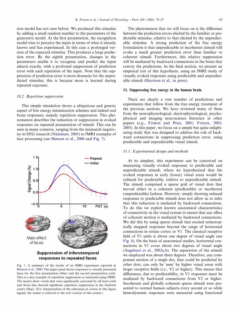
This simple simulation shows a ubiquitous and genericaspect of free energy minimisation schemes and indeed realbrain responses; namely repetition suppression. This phe-nomenon describes the reduction or suppression in evokedresponses on repeated presentation of stimuli. This can beseen in many contexts, ranging from the mismatch negativ-ity in EEG research (Naatanen, 2003) to fMRI examples offace processing (see Henson et al., 2000 and Fig. 7).

Fig. 7. A summary of the results of an fMRI experiment reported inHenson et al., 2000. The upper panel shows responses to visually presentedfaces for the first presentation (blue) and the second presentation (red).This is a nice example of repetition suppression as measured using fMRI.The inserts show voxels that were significantly activated by all faces (red)and those that showed significant repetition suppression in the fusiformcortex (blue). (For interpretation of the references in colour in this figurelegend, the reader is referred to the web version of this article.)

The phenomenon that we will focus on is the differencebetween the prediction errors elicited by the familiar or pre-dictable stimulus, relative to that elicited by the unpredict-able stimulus. A strong prediction of the free energyformulation is that unpredictable or incoherent stimuli willevoke a much greater prediction error than familiar orcoherent stimuli. Furthermore, this relative suppressionwill be mediated by backward connections in the brain thatconvey the predictions. In the final section, we present anempirical test of this hypothesis, using an fMRI study ofvisually evoked responses using predictable and unpredict-able stimuli (Harrison et al., in press).

11. Suppressing free energy in the human brain

There are clearly a vast number of predictions andexperiments that follow from the free energy treatment ofthe previous sections. We have reviewed many of thesefrom the neurophysiological, electrophysiological, psycho-physical and imaging neuroscience literature in otherpapers (e.g., Friston and Price, 2001; Friston, 2003,2005). In this paper, we focus on a simple but quite enlight-ening study that was designed to address the role of back-ward connections in suppressing prediction error, usingpredictable and unpredictable visual stimuli.

11.1. Experimental design and methods

At its simplest, this experiment can be conceived onmeasuring visually evoked responses to predictable andunpredictable stimuli, where we hypothesized that theevoked responses in early (lower) visual areas would bereduced for predictable, relative to unpredictable stimuli.The stimuli comprised a sparse grid of visual dots thatmoved either in a coherent (predictable) or incoherent(unpredictable) fashion. However, simply showing reducedresponses to predictable stimuli does not allow us to inferthat this reduction is mediated by backward connections.To do this we exploit known anatomical characteristicsof connectivity in the visual system to ensure that any effectof coherent motion is mediated by backward connections.We did this by using sparse stimuli that excited retinotop-ically mapped responses beyond the range of horizontalconnections in striate cortex or V1. The classical receptivefield of V1 units is about one degree of visual angle (seeFig. 8). On the basis of anatomical studies, horizontal con-nections in V1 cover about two degrees of visual angle(Angelucci et al., 2002a,b). The separation of the stimuliwe employed was about three degrees. Therefore, any com-ponent motion of a single dot, that could be predicted byother dots, can only be ‘seen’ by higher visual areas withlarger receptive fields (i.e., V2 or higher). This means thatdifferences, due to predictability, in V1 responses must bemediated by backward connections from V2 or higher.Incoherent and globally coherent sparse stimuli were pre-sented to normal human subjects every second or so whilehemodynamic responses were measured using functional

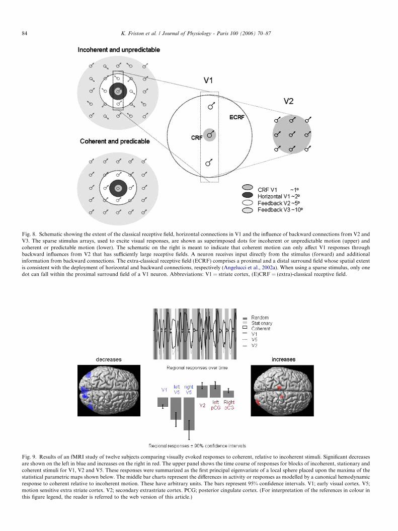
Fig. 8. Schematic showing the extent of the classical receptive field, horizontal connections in V1 and the influence of backward connections from V2 andV3. The sparse stimulus arrays, used to excite visual responses, are shown as superimposed dots for incoherent or unpredictable motion (upper) andcoherent or predictable motion (lower). The schematic on the right is meant to indicate that coherent motion can only affect V1 responses throughbackward influences from V2 that has sufficiently large receptive fields. A neuron receives input directly from the stimulus (forward) and additionalinformation from backward connections. The extra-classical receptive field (ECRF) comprises a proximal and a distal surround field whose spatial extentis consistent with the deployment of horizontal and backward connections, respectively (Angelucci et al., 2002a). When using a sparse stimulus, only onedot can fall within the proximal surround field of a V1 neuron. Abbreviations: V1 = striate cortex, (E)CRF = (extra)-classical receptive field.

Fig. 9. Results of an fMRI study of twelve subjects comparing visually evoked responses to coherent, relative to incoherent stimuli. Significant decreasesare shown on the left in blue and increases on the right in red. The upper panel shows the time course of responses for blocks of incoherent, stationary andcoherent stimuli for V1, V2 and V5. These responses were summarized as the first principal eigenvariate of a local sphere placed upon the maxima of thestatistical parametric maps shown below. The middle bar charts represent the differences in activity or responses as modelled by a canonical hemodynamicresponse to coherent relative to incoherent motion. These have arbitrary units. The bars represent 95% confidence intervals. V1; early visual cortex. V5;motion sensitive extra striate cortex. V2; secondary extrastriate cortex. PCG; posterior cingulate cortex. (For interpretation of the references in colour inthis figure legend, the reader is referred to the web version of this article.)



magnetic resonance imaging. The data were analysed usingconventional statistical parametric mapping. This involvedmodelling evoked responses with a stimulus functionencoding the occurrence of coherent or incoherent stimuliand convolving these with a hemodynamic response func-tion to form regressors for a general linear model. Infer-ences about differential responses between coherent andincoherent stimuli were assessed using a single-sample t-testover subjects, on appropriate contrasts from each subject.The results of this random effects analysis are shown inFig. 9.

11.2. Results

As predicted, there were profound reductions in visuallyevoked responses to predictable, relative to incoherent,visual stimuli in V1. Interestingly, these decreases were alsoseen in V5, bilaterally. The time course of hemodynamicactivity for a single subject is shown in the upper panelfor V1, V2 and V5. This graphic also shows the estimatedresponses to control stimuli that did not move. Again, aspredicted, enhanced responses to unpredictable stimuliwas seen at the first level that the receptive fields couldencompass more than one dot. This was in area V2. Thismay reflect the activity of deep pyramidal cells encodingglobal motion subtended by multiple dots. It is interestingto note that V5 showed a reduced prediction error, despitethe fact that this area is generally thought to be hierarchi-cally higher in the visual cortex than V2. However, extra-geniculate pathways can bypass V1 and V2 and provideinformation directly to V5 which, in some circumstances,may make it behave like a hierarchically low area. This isconsistent with the short-latency responses of V5, in rela-tion to V1 (see Nowak and Bullier, 1997).

In summary, this fMRI study confirms our predictionsfrom the theoretical analysis that evoked responses aresmaller for predictable, relative to unpredictable stimuli.This is consistent with measured responses reflecting, inlarge part, prediction error evoked as the sensory cortexself-organises to infer the causes of its geniculate input.Furthermore, by careful design of the stimuli to precludehorizontal interactions among V1 units, we are able to inferthat this suppression of prediction error has to be mediatedby backward connections from higher cortical areas. Thisis consistent with the recurrent dynamics entailed by thehierarchical formulation of generative models in the brainand the inversion of these models in accord with the freeenergy principle.

12. Conclusion

In this paper, we have considered the characteristics ofbiological systems, in relation to non-biological self-orga-nizing and dissipative systems. Biological systems act onthe environment and can sample it selectively to avoidphase-transitions that will irreversibly alter their structure.This adaptive exchange can be formalised in terms of free

energy minimisation, in which both the behaviour of theorganism and its internal configuration minimise its freeenergy. This free energy is a function of the ensemble den-sity encoded by the organism’s configuration and the sen-sory data to which it is exposed. Minimisation of freeenergy occurs through action-dependent changes in sen-sory input and the ensemble density implied by internalchanges. Systems that fail to maintain a low free energy willencounter phase-transitions as their relationship to theenvironment changes. It is therefore necessary, if not suffi-cient, for biological systems to minimise their free energy.

This free energy is not a thermodynamic free energy buta free energy formulated in terms of information theoreticquantities. The free energy principle discussed here is not aconsequence of thermodynamics but arises from popula-tion dynamics and selection. Put simply, systems with alow free energy will be selected over systems with a higherfree energy. The free energy rests on a specification of agenerative model, which is entailed by the organism’s struc-ture. Identifying this model enables one to predict how asystem will change if it conforms to the free energy princi-ple. For the brain, a plausible model is a hierarchicaldynamic system in which neural activity encodes the condi-tional modes of environmental states and its connectivityencodes the causal context in which these states evolve.Bayesian inversion of this model, to infer the causes of sen-sory input, is a natural consequence of minimising freeenergy or, under simplifying assumptions, the suppressionof prediction error. We concluded with a simple but com-pelling experiment that showed the relative suppressionof prediction error, in the context of predictable stimuli,is indeed mediated by backward connections in the brainas predicted by a free energy descent scheme.

The ideas presented in this paper have a deep history;starting with the notions of neuronal energy described byHelmholtz (1860) and covering ideas like analysis by syn-thesis (Neisser, 1967) and more recent formulations likeBayesian inversion and predictive coding (e.g., Ballardet al., 1983; Mumford, 1992; Dayan et al., 1995; Rao andBallard, 1998). The specific contribution of this paper isto provide a general formulation of the free energy princi-ple to cover both action and perception. Furthermore, thisformulation can be used to connect constructs frommachine learning and statistical physics with selectionistideas from theoretical biology.

Acknowledgements

The Wellcome Trust funded this work. We would like toexpress our greatest thanks to Marcia Bennett for prepar-ing this manuscript.

Appendix A. The conditional covariances

Under the Laplace approximation, the variational den-sity assumes a Gaussian form qi = N(li,Ri) with variational


parameters li and Ri, corresponding to the conditionalmode and covariance of the ith parameter set. The advan-tage of this approximation is that the conditional covari-ance can be evaluated very simply: Under the Laplaceapproximation the free energy is

F ¼ LðlÞ þ 1

2

Xi

ðU i þ ln jRij þ pi ln 2peÞ

U i ¼ trðRio2LðlÞ=o#io#iÞ

Lð#Þ ¼ ln pð~y; #Þ

Ið#iÞ ¼ Lð#i; lniÞ þ1

2

Xj 6¼i

U j

ðA:1Þ

pi is the number of parameters in the ith set. The condi-tional covariances obtain as an analytic function of themodes by differentiating the free energy and solving forzero

oF =oRi ¼1

2o2LðlÞ=o#io#i þ

1

2R�1

i ¼ 0

) R�1i ¼ �o2LðlÞ=o#io#i ðA:2Þ

This solution for the conditional covariances does not de-pend on the mean-field approximation but only on the La-place approximation. See Friston et al. (in press) for moredetails.

Appendix B. Dynamic models

Here we consider the functional form of the generativedensity for hierarchical dynamic models of the sort descriedin Eq. (10). To simplify things, we will deal with a singlelevel and generalise to multiple levels later

y ¼ gðx; vÞ þ z

_x ¼ f ðx; vÞ þ wðA:3Þ

The continuous non-linear functions f(x,v) and g(x,v) ofstates are parameterised by #h. Stochastic innovations z(t)are assumed to be analytic such that the covariance of~z ¼ z; z0; z00; . . . is well defined in generalised coordinates;similarly for random fluctuations in the states, ~w. Under lo-cal linearity assumptions, the generalised motion ~y is givenby

y ¼ gðx; vÞ þ z x0 ¼ f ðx; vÞ þ w

_y ¼ gxx0 þ gvv

0 þ z0 x00 ¼ fxx0 þ fvv0 þ w0

€y ¼ gxx00 þ gvv

00 þ z00 x000 ¼ fxx00 þ fvv00 þ w00

..

. ...

ðA:4Þ

This model induces a variational density q(#u, t) on the gen-eralised causes #u ¼ ~x;~v. The second set of equations pre-scribes dynamics by coupling low and high-order motionof x(t), which confers memory on the system. Gaussianassumptions about the fluctuations furnish the functionalform of the likelihood pð~yj#Þ ¼ Nð~g;P�1

z Þ, where ~g and ~fcomprise the generalised predictions

g ¼ gðx; vÞ f ¼ f ðx; vÞg0 ¼ gxx

0 þ gvv0 f 0 ¼ fxx0 þ fvv0

g00 ¼ gxx00 þ gvv

00 f 00 ¼ fxx00 þ fvv00

..

. ...

ðA:5Þ

P(#c)z is the precision (i.e., inverse covariance) of ~z thatcontrols its amplitude and roughness. Similarly, Gaussianassumptions about fluctuations in the states allow us to ex-press the prior pð#uÞ ¼ pð~xj~vÞpð~vÞ in terms of predicted mo-tion, where pð~xj~vÞ ¼ Nð~f ;P�1

w Þ and P(#c)w is the precisionof ~w. We now have now the functional form of the likeli-hood and priors and implicitly the generative model.

Adding hierarchical levels, with y = v(0) gives Eq. (10)

vði�1Þ ¼ gðxðiÞ; vðiÞÞ þ zðiÞ

_xðiÞ ¼ f ðxðiÞ; vðiÞÞ þ wðiÞðA:6Þ

These induce empirical priors on the states that lend thegenerative density a Markov form, through independenceassumptions (Kass and Steffey, 1989) about the randomfluctuations in different levels

pð~y; #Þ ¼ pð~yj#ð1Þu Þpð#ð1Þu j#

ð2Þu Þ � � � pð~vðmÞÞ

p #ði�1Þu j#ðiÞu

� �¼ p ~xði�1Þj~vði�1Þ� �

p ~vði�1Þj#ðiÞu

� �p ~xðiÞj~vðiÞ� �

¼ N ~f ðiÞ;PðiÞ�1w

� �p ~vði�1Þj#ðiÞu

� �¼ N ~gðiÞ;PðiÞ�1

z

� �ðA:7Þ

The prediction ~gð#ðiÞu ; #ðiÞh Þ plays the role of a prior expecta-

tion on ~vði�1Þ and its prior precision is estimated empiricallyas Pð#ðiÞc Þv; hence empirical Bayes (Efron and Morris,1973); similarly for the hidden states. In short, a hierarchi-cal form endows a model with the ability to construct itsown priors. This feature is central to many inference andestimation procedures ranging from mixed-effects analysesin classical covariance component analysis to automaticrelevance determination. See Friston et al., in press for afuller discussion of static models.

References

Angelucci, A., Levitt, J.B., Walton, E.J., Hupe, J.M., Bullier, J., Lund,J.S., 2002a. Circuits for local and global signal integration in primaryvisual cortex. J. Neurosci. 22, 8633–8646.

Angelucci, A., Levitt, J.B., Lund, J.S., 2002b. Anatomical origins of theclassical receptive field and modulatory surround field of singleneurons in macaque visual cortical area V1. Prog. Brain Res. 136,373–388.

Ashby, W.R., 1947. Principles of the self-organising dynamic system. J.Gen. Psychol. 37, 125–128.

Ballard, D.H., Hinton, G.E., Sejnowski, T.J., 1983. Parallel visualcomputation. Nature 306, 21–26.

Dayan, P., Hinton, G.E., Neal, R.M., 1995. The Helmholtz machine.Neural Comput. 7, 889–904.

DeFelipe, J., Alonso-Nanclares, L., Arellano, J.I., 2002. Microstructure ofthe neocortex: comparative aspects. J. Neurocytol. 31, 299–316.

Dempster, A.P., Laird, N.M., Rubin, D.B., 1977. Maximum likelihoodfrom incomplete data via the EM algorithm. J. Roy. Stat. Soc. Ser. B39, 1–38.


Edelman, G.M., 1993. Neural Darwinism: selection and reentrantsignaling in higher brain function. Neuron 10, 115–125.

Efron, B., Morris, C., 1973. Stein’s estimation rule and its competitors –an empirical Bayes approach. J. Am. Stat. Assoc. 68, 117–130.

Felleman, D.J., Van Essen, D.C., 1991. Distributed hierarchical process-ing in the primate cerebral cortex. Cerebral Cortex 1, 1–47.

Feynman, R.P., 1972. Statistical Mechanics. Benjamin, Reading MA,USA.

Friston, K.J., 2003. Learning and inference in the brain. Neural Networks16, 1325–1352.

Friston, K.J., 2005. A theory of cortical responses. Philos. Trans. R Soc.Lond. B Biol. Sci. 360, 815–836.

Friston, K.J., in preparation. DEM: a variational treatment of dynamicsystems.

Friston, K.J., Price, C.J., 2001. Dynamic representations and generativemodels of brain function. Brain Res. Bull. 54, 275–285.

Friston, K.J., Tononi, G., Reeke Jr., G.N., Sporns, O., Edelman, G.M.,1994. Value-dependent selection in the brain: simulation in a syntheticneural model. Neuroscience 59, 229–243.

Friston, K., Mattout, J., Trujillo-Barreto, N., Ashburner, J., Penny, W.,in press. Variational free energy and the Laplace approximation.NeuroImage.

Haken, H., 1983. Synergistics: An introduction. Non-equilibrium PhaseTransition and Self-organisation in Physics, Chemistry and Biology,third ed. Springer Verlag.

Harrison, L.M., Stephan, K.E., Rees, G., Friston, K.J., in press. Extra-classical receptive field effects measured in striate cortex with fMRI.NeuroImage.

Harville, D.A., 1977. Maximum likelihood approaches to variancecomponent estimation and to related problems. J. Am. Stat. Assoc.72, 320–338.

Helmholtz, H., 1860. Handbuch der physiologischen optik, vol. 3. Dover,New York (English trans., Southall JPC, Ed.).

Henson, R., Shallice, T., Dolan, R., 2000. Neuroimaging evidence fordissociable forms of repetition priming. Science 287, 1269–1272.

Hinton, G.E., von Cramp, D., 1993. Keeping neural networks simple byminimising the description length of weights. In: Proceedings ofCOLT-93, pp. 5–13.

Hochstein, S., Ahissar, M., 2002. View from the top: hierarchies andreverse hierarchies in the visual system. Neuron 36, 791–804.

Kass, R.E., Steffey, D., 1989. Approximate Bayesian inference inconditionally independent hierarchical models (parametric empiricalBayes models). J. Am. Stat. Assoc. 407, 717–726.

Kauffman, S., 1993. Self-organisation on Selection in Evolution. OxfordUniversity Press, Oxford, UK.

Kawato, M., Hayakawa, H., Inui, T., 1993. A forward-inverse opticsmodel of reciprocal connections between visual cortical areas.Network 4, 415–422.

Kersten, D., Mamassian, P., Yuille, A., 2004. Object perception asBayesian inference. Annu. Rev. Psychol. 55, 271–304.

Kording, K.P., Wolpert, D.M., 2004. Bayesian integration in sensorimo-tor learning. Nature 427, 244–247.

Kloucek, P., 1998. The computational modeling of nonequilibriumthermodynamics of the martensitic transformations. Comput. Mech.23, 239–254.

MacKay, D.M., 1956. The epistemological problem for automata. In:Shannon, C.E., McCarthy, J. (Eds.), Automata Studies. PrincetonUniversity Press, Princeton, NJ, pp. 235–251.

MacKay, D.J.C., 1995. Free energy minimisation algorithm for decodingand cryptoanalysis. Electron. Lett. 31, 445–447.

Maniadakis, M., Trahanias, P., 2006. Modelling brain emergent behav-iours through coevolution of neural agents. Neural Networks 19, 705–720.

Martinez-Trujillo, J.C., Treue, S., 2004. Feature-based attention increasesthe selectivity of population responses in primate visual cortex. Curr.Biol. 14, 744–751.

Mesulam, M.M., 1998. From sensation to cognition. Brain 121, 1013–1052.Montague, P.R., Dayan, P., Person, C., Sejnowski, T.J., 1995. Bee

foraging in uncertain environments using predictive Hebbian learning.Nature 377, 725–728.

Mumford, D., 1992. On the computational architecture of the neocortex.II. The role of cortico-cortical loops. Biol. Cybern. 66, 241–251.

Murphy, P.C., Sillito, A.M., 1987. Corticofugal feedback influences thegeneration of length tuning in the visual pathway. Nature 329, 727–729.

Naatanen, R., 2003. Mismatch negativity: clinical research and possibleapplications. Int. J. Psychophysiol. 48, 179–188.

Neal, R.M., Hinton, G.E., 1998. A view of the EM algorithm that justifiesincremental sparse and other variants. In: Jordan, M.I. (Ed.), Learningin Graphical Models. Kulver Academic Press.

Neisser, U., 1967. Cognitive Psychology. Appleton-Century-Crofts, NewYork.

Nicolis, G., Prigogine, I., 1977. Self-organisation in Non-equilibriumSystems. John Wiley, New York, USA, p. 24.

Nowak, L.G., Bullier, J., 1997. The timing of information transfer in thevisual system. Cereb. Cortex. 12, 205–241.

Prince, A., Smolensky, P., 1997. Optimality: from neural networks touniversal grammar. Science 275, 1604–1610.

Rao, R.P., 2005. Bayesian inference and attentional modulation in thevisual cortex. Neuro Rep. 16, 1843–1848.

Rao, R.P., Ballard, D.H., 1998. Predictive coding in the visual cortex: afunctional interpretation of some extra-classical receptive field effects.Nature Neurosci. 2, 79–87.

Rockland, K.S., Pandya, D.N., 1979. Laminar origins and terminations ofcortical connections of the occipital lobe in the rhesus monkey. BrainRes. 179, 3–20.

Sherman, S.M., Guillery, R.W., 1998. On the actions that one nerve cellcan have on another: distinguishing ‘‘drivers’’ from modulators. Proc.Natl. Acad. Sci. USA 95, 7121–7126.

Schroeder, C.E., Mehta, A.D., Foxe, J.J., 2001. Determinants andmechanisms of attentional modulation of neural processing. FrontBiosci. 6, D672–D684.

Suri, R.E., Schultz, W., 2001. Temporal difference model reproducesanticipatory neural activity. Neural Comput. 13, 841–862.

Treue, S., Maunsell, H.R., 1996. Attentional modulation of visual motionprocessing in cortical areas MT and MST. Nature 382, 539–541.

Yu, A.J., Dayan, P., 2005. Uncertainty, neuromodulation and attention.Neuron 46, 681–692.

Zeki, S., Shipp, S., 1988. The functional logic of cortical connections.Nature 335, 311–317.

a free energy principle for the brainkarl/a free energy principle for the brain.pdf · a free...

Documents