A Faster Algorithm for Computing Straight

Skeletons

Thesis by

Liam Mencel

In Partial Fulfilment of the Requirements

For the Degree of

Masters of Science

King Abdullah University of Science and Technology, Thuwal,

Kingdom of Saudi Arabia

May, 2014

2

The thesis of Liam Mencel is approved by the examination committee.

Committee Chairperson: Antoine Vigneron

Committee Member: Mikhail Moshkov

Committee Member: Markus Hadwiger

3

Copyright ©2014

Liam Mencel

All Rights Reserved

4

ABSTRACT

A Faster Algorithm for Computing Straight Skeletons

Liam Mencel

We present a new algorithm for computing the straight skeleton of a polygon.

For a polygon with n vertices, among which r are reflex vertices, we give a de-

terministic algorithm that reduces the straight skeleton computation to a motor-

cycle graph computation in O(n(log n) log r) time. It improves on the previously

best known algorithm for this reduction, which is randomised, and runs in expected

O(n√h+ 1 log2 n) time for a polygon with h holes. Using known motorcycle graph

algorithms, our result yields improved time bounds for computing straight skeletons.

In particular, we can compute the straight skeleton of a non-degenerate polygon in

O(n(log n) log r + r4/3+ε) time for any ε > 0. On degenerate input, our time bound

increases to O(n(log n) log r + r17/11+ε).

5

ACKNOWLEDGEMENTS

I would like to express gratitude towards my supervisor, Professor Antoine Vigneron

for his expertise and support over the past year, in particular for the significant time

he put into handling the formatting and submission of our paper.

I also wish to thank Professor Siu-Wing Cheng, who helped me settle into Hong

Kong over the summer period and supported me in the early stages of this research

during that time.

Finally, I must acknowledge my colleague and friend Mohammed Al Farhan, an

MSc student who worked with me on many important projects during my time in

KAUST. His assistance was a great help in getting me through the degree program

and affording me more time to focus on my thesis.

6

TABLE OF CONTENTS

Examination Committee Approval 2

Copyright 3

Abstract 4

Acknowledgements 5

List of Figures 7

List of Tables 8

1 Introduction 9

2 Notations and preliminaries 13

3 Computing the vertical subdivision 18

3.1 Subdivision induced by a vertical cut . . . . . . . . . . . . . . . . . . 18

3.2 Data structure . . . . . . . . . . . . . . . . . . . . . . . . . . . . . . . 21

3.3 Algorithm . . . . . . . . . . . . . . . . . . . . . . . . . . . . . . . . . 23

3.4 Analysis . . . . . . . . . . . . . . . . . . . . . . . . . . . . . . . . . . 26

4 Cutting between valleys 32

4.1 Algorithm . . . . . . . . . . . . . . . . . . . . . . . . . . . . . . . . . 32

4.2 Analysis . . . . . . . . . . . . . . . . . . . . . . . . . . . . . . . . . . 34

5 Summary 37

5.1 Degenerate cases . . . . . . . . . . . . . . . . . . . . . . . . . . . . . 37

5.2 Tightness of analysis . . . . . . . . . . . . . . . . . . . . . . . . . . . 38

5.3 Future Research Work . . . . . . . . . . . . . . . . . . . . . . . . . . 39

References 41

7

LIST OF FIGURES

1.1 The straight skeleton is obtained by shrinking the input polygon P . . 9

2.1 Illustration of the two different types of slabs. (a) The terrain T , an

edge slab and motorcycle slab. This terrain has two valleys, adjacent

to the two reflex vertices of the polygon. (b) The motorcycle graph Gassociated with P and the boundaries of the edge slab and the motor-

cycle slab viewed from above. . . . . . . . . . . . . . . . . . . . . . . 14

2.2 Motorcycle graph. . . . . . . . . . . . . . . . . . . . . . . . . . . . . . 15

2.3 The polygon P , its skeletons and descent paths. . . . . . . . . . . . . 16

3.1 Empty cells and a wedge. . . . . . . . . . . . . . . . . . . . . . . . . . 21

3.2 The face lists for the cell Ci bounded by the vertical line cuts `−i and

`+i . The faces are denoted by f1, . . . , f19 and the corresponding slabs

are σ1, . . . , σ19. The face lists point to these slabs, as the exact shape

of the faces of S ′ is not known. . . . . . . . . . . . . . . . . . . . . . 29

3.3 A first wedge is created (left), and an adjacent wedges is created after-

wards (right). The cell containing p has been split simultaneously. . . 30

3.4 The vertical subdivision. (Continued in Figure 4.2.) . . . . . . . . . 31

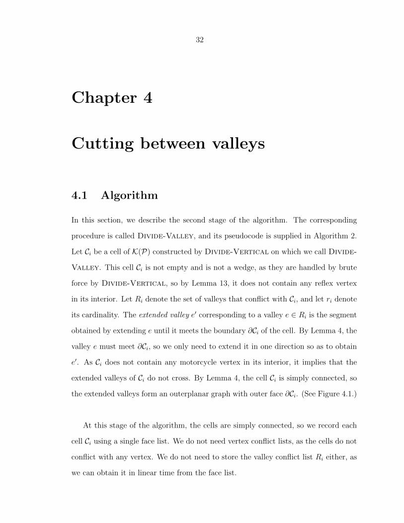
4.1 (Left) The cell Ci and the conflicting valleys. (Middle) The extended

valleys, and a balanced cut. (Right) The triangulation and its dual

graph. . . . . . . . . . . . . . . . . . . . . . . . . . . . . . . . . . . . 33

4.2 The result of the two stages of subdivision. . . . . . . . . . . . . . . . 36

5.1 Tight example. For vertical cuts that are introduced from left to right,

the four slabs corresponding to e1, e2, e3, e4 conflict with the cuts. . . 39

8

LIST OF TABLES

1.1 Summary of previously best known results, compared with those of our

new algorithm. . . . . . . . . . . . . . . . . . . . . . . . . . . . . . . 11

9

Chapter 1

Introduction

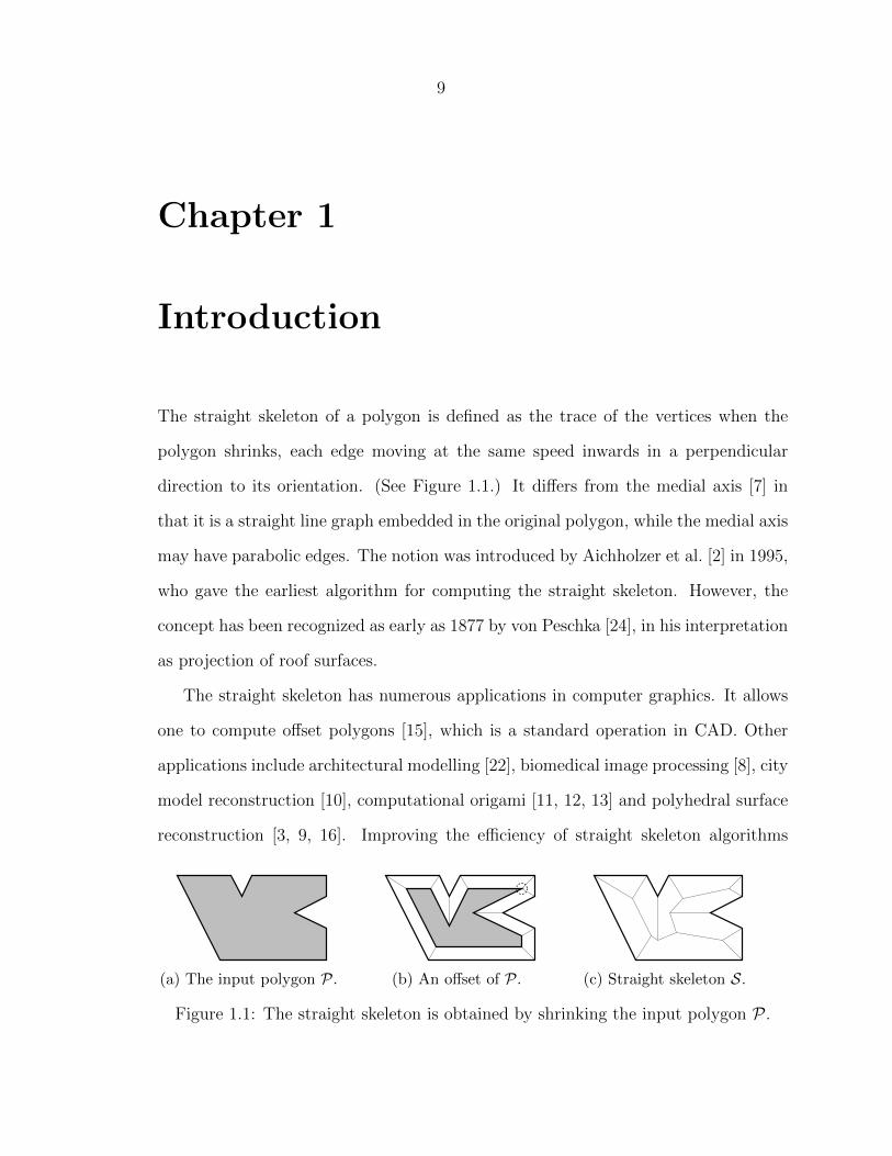
The straight skeleton of a polygon is defined as the trace of the vertices when the

polygon shrinks, each edge moving at the same speed inwards in a perpendicular

direction to its orientation. (See Figure 1.1.) It differs from the medial axis [7] in

that it is a straight line graph embedded in the original polygon, while the medial axis

may have parabolic edges. The notion was introduced by Aichholzer et al. [2] in 1995,

who gave the earliest algorithm for computing the straight skeleton. However, the

concept has been recognized as early as 1877 by von Peschka [24], in his interpretation

as projection of roof surfaces.

The straight skeleton has numerous applications in computer graphics. It allows

one to compute offset polygons [15], which is a standard operation in CAD. Other

applications include architectural modelling [22], biomedical image processing [8], city

model reconstruction [10], computational origami [11, 12, 13] and polyhedral surface

reconstruction [3, 9, 16]. Improving the efficiency of straight skeleton algorithms

(a) The input polygon P. (b) An offset of P. (c) Straight skeleton S.

Figure 1.1: The straight skeleton is obtained by shrinking the input polygon P .

10

increases the speed of related tools in geometric computing.

The first algorithm by Aichholzer et al. [2] runs in O(n2 log n) time, and simu-

lates the shrinking process discretely. Eppstein and Erickson [15] developed the first

sub-quadratic algorithm, which runs in O(n17/11+ε) time. In their work, they pro-

posed motorcycle graphs as a means of encapsulating the main difficulty in comput-

ing straight skeletons. Cheng and Vigneron [6] expanded on this notion by reducing

the straight skeleton problem in non-degenerate cases to a motorcycle graph com-

putation and a lower envelope computation. This reduction was later extended to

degenerate cases by Held and Huber [18]. Cheng and Vigneron gave an algorithm

for the lower envelope computation on a non-degenerate polygon with h holes, which

runs in O(n√h+ 1 log2 n) expected time. They also provided a method for solving the

motorcycle graph problem in O(n√n log n) time. Putting the two together gives an

algorithm which solves the straight skeleton problem in O(n√h+ 1 log2 n+r

√r log r)

expected time, where r is the number of reflex vertices.

Comparison with previous work. Recently, Vigneron and Yan [23] found a

faster, O(n4/3+ε)-time algorithm for computing motorcycle graphs. It thus removed

one bottleneck in straight skeleton computation. In this paper we remove the sec-

ond bottleneck: We give a faster reduction to the motorcycle graph problem. Our

algorithm performs this reduction in deterministic O(n(log n) log r) time, improving

on the previously best known algorithm, which is randomised and runs in expected

O(n√h+ 1 log2 n) time [6].

Using known algorithms for computing motorcycle graphs, our reduction yield

faster algorithms for computing the straight skeleton. In particular, using the al-

gorithm by Vigneron and Yan [23], we can compute the straight skeleton of a non-

degenerate polygon in O(n(log n) log r + r4/3+ε) time for any ε > 0. On degenerate

input, we use Eppstein and Erickson’s algorithm, and our time bound increases to

11

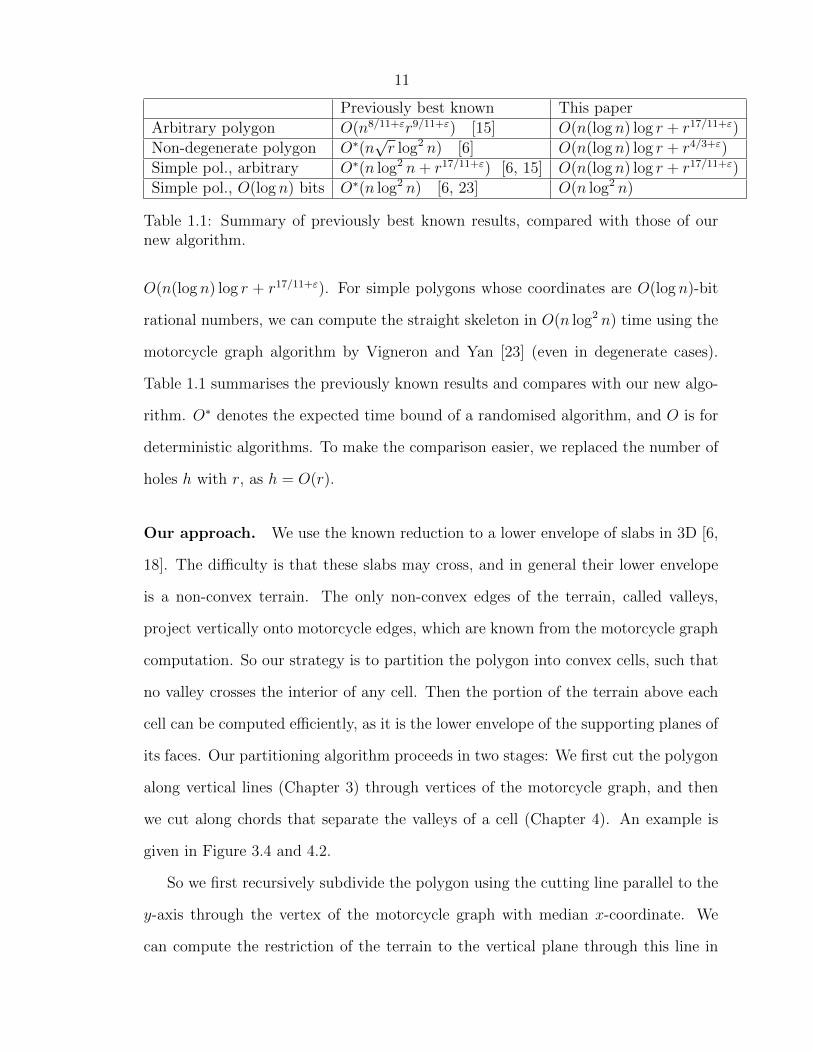
Previously best known This paper

Arbitrary polygon O(n8/11+εr9/11+ε) [15] O(n(log n) log r + r17/11+ε)

Non-degenerate polygon O∗(n√r log2 n) [6] O(n(log n) log r + r4/3+ε)

Simple pol., arbitrary O∗(n log2 n+ r17/11+ε) [6, 15] O(n(log n) log r + r17/11+ε)

Simple pol., O(log n) bits O∗(n log2 n) [6, 23] O(n log2 n)

Table 1.1: Summary of previously best known results, compared with those of ournew algorithm.

O(n(log n) log r + r17/11+ε). For simple polygons whose coordinates are O(log n)-bit

rational numbers, we can compute the straight skeleton in O(n log2 n) time using the

motorcycle graph algorithm by Vigneron and Yan [23] (even in degenerate cases).

Table 1.1 summarises the previously known results and compares with our new algo-

rithm. O∗ denotes the expected time bound of a randomised algorithm, and O is for

deterministic algorithms. To make the comparison easier, we replaced the number of

holes h with r, as h = O(r).

Our approach. We use the known reduction to a lower envelope of slabs in 3D [6,

18]. The difficulty is that these slabs may cross, and in general their lower envelope

is a non-convex terrain. The only non-convex edges of the terrain, called valleys,

project vertically onto motorcycle edges, which are known from the motorcycle graph

computation. So our strategy is to partition the polygon into convex cells, such that

no valley crosses the interior of any cell. Then the portion of the terrain above each

cell can be computed efficiently, as it is the lower envelope of the supporting planes of

its faces. Our partitioning algorithm proceeds in two stages: We first cut the polygon

along vertical lines (Chapter 3) through vertices of the motorcycle graph, and then

we cut along chords that separate the valleys of a cell (Chapter 4). An example is

given in Figure 3.4 and 4.2.

So we first recursively subdivide the polygon using the cutting line parallel to the

y-axis through the vertex of the motorcycle graph with median x-coordinate. We

can compute the restriction of the terrain to the vertical plane through this line in

12

near-linear time, as it reduces to computing a lower envelope of segments. Then the

descent paths from the vertices of this polyline are added as new cell boundaries, as

well as the intersection of the cutting line with the current cell. Each cell contains at

most half as many motorcycle vertices in its interior as its parent, hence the depth of

recursion is O(log r). Our data structure allows us to subdivide a cell in near linear

time, and a careful analysis shows that this first stage can be completed in overall

O(n(log n) log r) time.

Thus we obtain a partition such that no cell contains a motorcycle vertex in its

interior. It follows that within each cell, the motorcycle tracks corresponding to

the valleys are non-intersecting. We then partition recursively in the same way as

in the first stage, but using chords of the cell that separate the motorcycle tracks

in a balanced manner, instead of the lines parallel to the y-axis. The number of

valleys incident to a cell drops by a factor at least 3/2 at each subdivision, so the

depth of recursion is still O(log r). We can still perform the partitioning in overall

O(n(log n) log r) time, and we obtain a partition such that the terrain is convex above

each cell.

We state here the main result of this work:

Theorem 1. Given a polygon P with n vertices, r of which being reflex vertices, and

given the motorcycle graph induced by P, we can compute the straight skeleton of P

in O(n(log n) log r) time.

13

Chapter 2

Notations and preliminaries

The input polygon is denoted by P . It has n vertices, among which r are reflex

vertices. We work in R3 with P lying flat in the xy-plane. The z-axis becomes

analogous to the time dimension. We say that a line, or a line segment, is vertical,

if it is parallel to the y-axis, and we say that a plane is vertical if it is orthogonal to

the xy-plane. The boundary of a set A is denote by by ∂A. The cardinality of a set

A is denoted by |A|. We denote by pq the line segment with endpoints p, q. A reflex

vertex of a polygon is a vertex at which the internal angle is more than π.

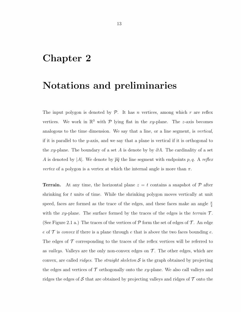
Terrain. At any time, the horizontal plane z = t contains a snapshot of P after

shrinking for t units of time. While the shrinking polygon moves vertically at unit

speed, faces are formed as the trace of the edges, and these faces make an angle π4

with the xy-plane. The surface formed by the traces of the edges is the terrain T .

(See Figure 2.1 a.) The traces of the vertices of P form the set of edges of T . An edge

e of T is convex if there is a plane through e that is above the two faces bounding e.

The edges of T corresponding to the traces of the reflex vertices will be referred to

as valleys. Valleys are the only non-convex edges on T . The other edges, which are

convex, are called ridges. The straight skeleton S is the graph obtained by projecting

the edges and vertices of T orthogonally onto the xy-plane. We also call valleys and

ridges the edges of S that are obtained by projecting valleys and ridges of T onto the

14

π4

(a) (b)

Figure 2.1: Illustration of the two different types of slabs. (a) The terrain T , anedge slab and motorcycle slab. This terrain has two valleys, adjacent to the tworeflex vertices of the polygon. (b) The motorcycle graph G associated with P and theboundaries of the edge slab and the motorcycle slab viewed from above.

xy-plane.

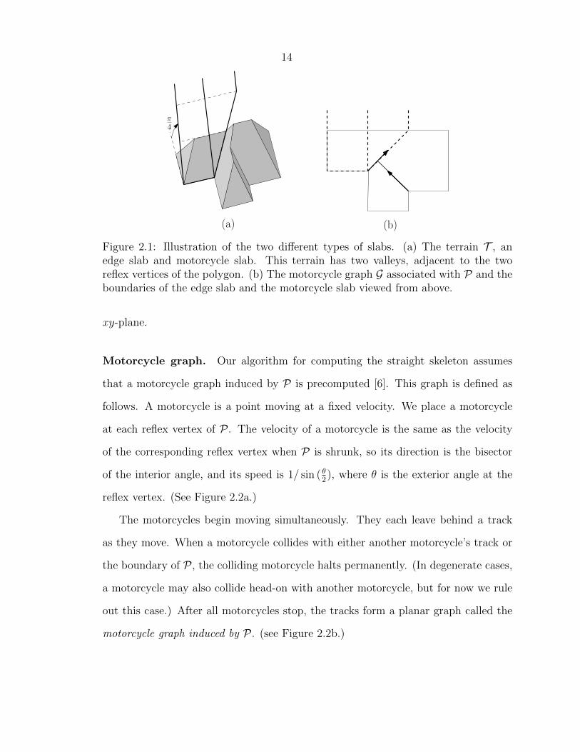
Motorcycle graph. Our algorithm for computing the straight skeleton assumes

that a motorcycle graph induced by P is precomputed [6]. This graph is defined as

follows. A motorcycle is a point moving at a fixed velocity. We place a motorcycle

at each reflex vertex of P . The velocity of a motorcycle is the same as the velocity

of the corresponding reflex vertex when P is shrunk, so its direction is the bisector

of the interior angle, and its speed is 1/ sin ( θ2), where θ is the exterior angle at the

reflex vertex. (See Figure 2.2a.)

The motorcycles begin moving simultaneously. They each leave behind a track

as they move. When a motorcycle collides with either another motorcycle’s track or

the boundary of P , the colliding motorcycle halts permanently. (In degenerate cases,

a motorcycle may also collide head-on with another motorcycle, but for now we rule

out this case.) After all motorcycles stop, the tracks form a planar graph called the

motorcycle graph induced by P . (see Figure 2.2b.)

15

θ1/ sin(θ2)

(a) (b)

Figure 2.2: Motorcycle graph.

General position assumptions. To simplify the description and the analysis of

our algorithm, we assume that the polygon is in general position. No edge of P or S

is vertical. No two motorcycles collide with each other in the motorcycle graph, and

thus each valley is adjacent to some reflex vertex. Each vertex in the straight skeleton

graph has degree 1 or 3. Our results, however, generalise to degenerate polygons, as

explained in Section 5.1.

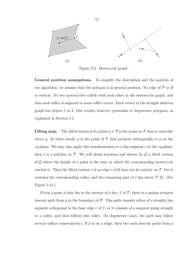
Lifting map. The lifted version p of a point p ∈ P is the point on T that is vertically

above p. In other words, p is the point of T that projects orthogonally to p on the

xy-plane. We may also apply this transformation to a line segment s in the xy-plane,

then s is a polyline in T . We will abuse notation and denote by G a lifted version

of G where the height of a point is the time at which the corresponding motorcycle

reaches it. Then the lifted version e of an edge e of G does not lie entirely on T , but it

contains the corresponding valley, and the remaining part of e lies above T [6]. (See

Figure 2.1a.)

Given a point p that lies in the interior of a face f of T , there is a unique steepest

descent path from p to the boundary of P . This path consists either of a straight line

segment orthogonal to the base edge e of f , or it consists of a segment going straight

to a valley, and then follows this valley. (In degenerate cases, the path may follow

several valleys consecutively.) If p is on a ridge, then two such descent paths from p

16

(a) The skeleton S. (b) The skeleton S ′. (c) Descent paths.

Figure 2.3: The polygon P , its skeletons and descent paths.

exist, and if p is a convex vertex, then there are three such paths. (See Figure 2.3c.)

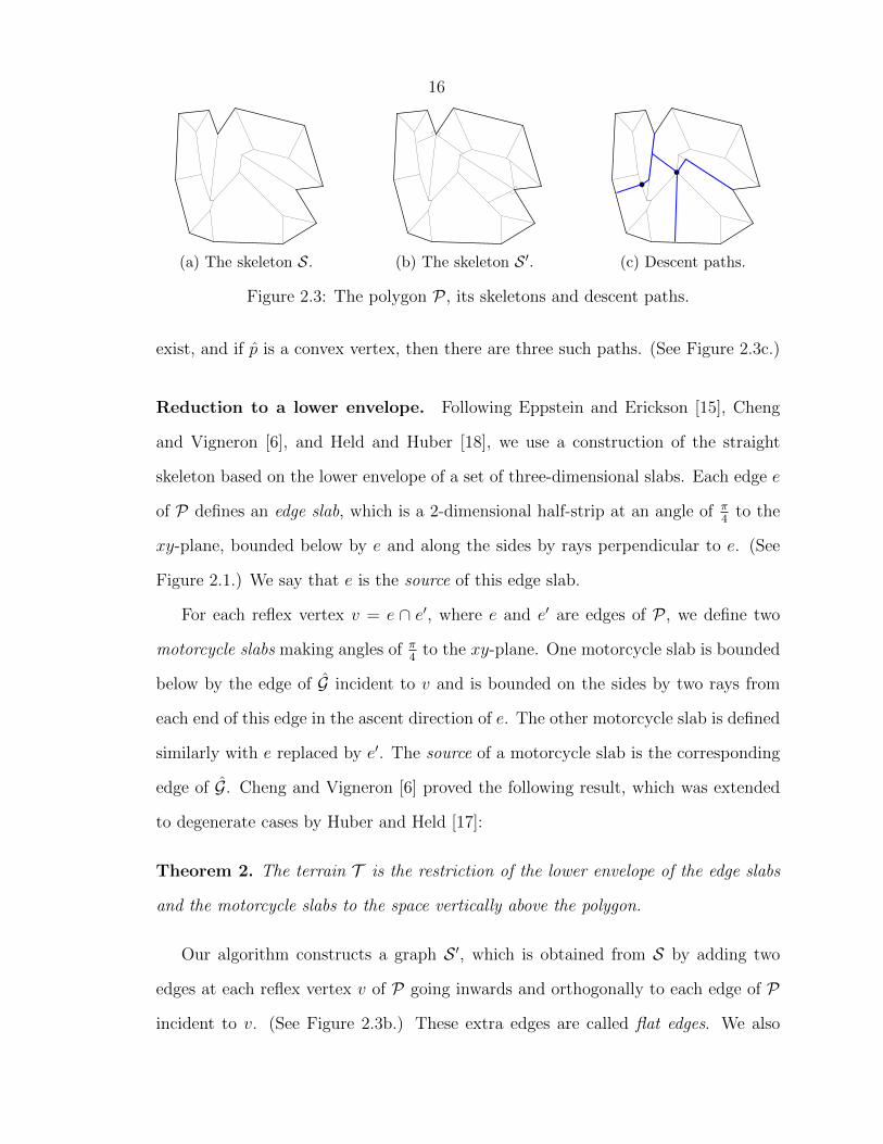
Reduction to a lower envelope. Following Eppstein and Erickson [15], Cheng

and Vigneron [6], and Held and Huber [18], we use a construction of the straight

skeleton based on the lower envelope of a set of three-dimensional slabs. Each edge e

of P defines an edge slab, which is a 2-dimensional half-strip at an angle of π4

to the

xy-plane, bounded below by e and along the sides by rays perpendicular to e. (See

Figure 2.1.) We say that e is the source of this edge slab.

For each reflex vertex v = e ∩ e′, where e and e′ are edges of P , we define two

motorcycle slabs making angles of π4

to the xy-plane. One motorcycle slab is bounded

below by the edge of G incident to v and is bounded on the sides by two rays from

each end of this edge in the ascent direction of e. The other motorcycle slab is defined

similarly with e replaced by e′. The source of a motorcycle slab is the corresponding

edge of G. Cheng and Vigneron [6] proved the following result, which was extended

to degenerate cases by Huber and Held [17]:

Theorem 2. The terrain T is the restriction of the lower envelope of the edge slabs

and the motorcycle slabs to the space vertically above the polygon.

Our algorithm constructs a graph S ′, which is obtained from S by adding two

edges at each reflex vertex v of P going inwards and orthogonally to each edge of P

incident to v. (See Figure 2.3b.) These extra edges are called flat edges. We also

17

include the edges of P into S ′. It means that each face f of S ′ corresponds to exactly

one slab. More precisely, a face is the vertical projection of T ∩ σ to the xy-plane

for some slab σ. By contrast, in the original straight skeleton S, a face incident to a

reflex vertex corresponds to one edge slab and one motorcycle slab.

18

Chapter 3

Computing the vertical subdivision

In this section, we describe and we analyse the first stage of our algorithm, where

the input polygon P is recursively partitioned using vertical cuts. The corresponding

procedure is called Divide-Vertical, and its pseudocode can be found in Algo-

rithm 1. It results in a subdivision of the input polygon P , such that any cell of

this subdivision has the following property: It does not contain any vertex of G in its

interior, or it is contained in the union of two faces of S ′. The second stage of our

algorithm is presented in Chapter 4.

3.1 Subdivision induced by a vertical cut

At any step of the algorithm, we maintain a planar subdivision K(P), which is a

partition of the input polygon P into polygonal cells. Each cell is a polygon, hence

it is connected. A cell C in the current subdivision K(P) may be further subdivided

as follows.

Let ` be a vertical line through a vertex of G. We assume that ` intersects C,

and hence C ∩ ` consists of several line segments s1, . . . , sq. These line segments are

introduced as new boundary edges in K(P); they are called the vertical edges of K(P).

They may be further subdivided during the course of the algorithm, and we still call

the resulting edges vertical edges.

19

Then we insert non-vertical edges along steepest descent paths, as follows. Each

intersection point p ∈ sj ∩ S ′ has a lifted version p on T . By our non-degeneracy

assumptions, there are at most three steepest descent paths to ∂C from p. The

vertical projections of these paths onto C are also inserted as new edges in K(P). The

resulting partition of C is the subdivision induced by `. (See Figure 3.4.)

We denote by C1, C2, . . . the cells of K(P) that are constructed during the course

of the algorithm. Let `−i and `+i denote the vertical lines through the leftmost and

rightmost point of Ci, respectively. When we perform one step of the subdivision,

each new cell lies entirely to the left or to the right of the splitting line, and thus by

induction, any vertical edge of a cell Ci either lies in `−i or `+i . We now study the

geometry of these cells.

Lemma 3. Let p be a reflex vertex of a cell Ci. Then p is a reflex vertex of P such

that ∂Ci and ∂P coincide in a neighbourhood of p, or p is a point where a descent

path bounding Ci reaches a valley.

Proof. We prove it by induction. The initial cell is C1 = P , and hence the property

holds. When we perform a subdivision of a cell Ci along a line `, we cannot introduce

reflex vertices along `, as we insert the segments Ci ∩ ` as new cell boundaries. So

new reflex vertices may only appear along descent paths. They cannot appear at the

lower endpoint of a descent path, as a descent path can only meet a reflex vertex

along its exterior angle bisector. So a reflex vertex may only appear in the interior of

a descent path, and a descent path only bends when it reaches a valley.

The lemma above shows that non-convexity may only be introduced when a

bounding path reaches a valley. The lemma below implies that, at any point in

time, it can occur only once per valley. (See Figure 3.4.)

Lemma 4. Let e = pq be a valley or a flat edge of S ′, with p being a reflex vertex of P

and q being the other endpoint of e. At any time during the course of the algorithm,

20

there is a point a along e such that pa is contained in the union of the boundaries of

the cells of K(P), and the interior of aq is contained in the interior of a cell Ci.

Proof. We proceed by induction, so we assume that at the current point of the ex-

ecution of the algorithm, there is a point a on e such that pa is contained in the

union of the edges of K(P), and aq is contained in the interior of a cell Cj. So e

can only intersect the interior of a new cell if this cell is obtained by subdividing Cj.

When performing this subdivision, at most two descent paths and one vertical cut

can intersect aq, and then the descent paths from these intersection points to a are

added as cell boundaries. After that, we are again in the situation where e is split

into two segments pb and bq, with pb being covered by edges of K(P) and bq being in

the interior of a cell.

A ridge, on the other hand, can cross the interior of several cells. But its inter-

section with any given cell is a single line segment:

Lemma 5. For any ridge e and any cell Ci, the intersection e ∩ Ci is a single line

segment, and e ∩ Ci consists of at most two points.

Proof. As e is a convex edge, the only descent paths that can meet e are descent

paths that start from e. So e can only be partitioned by a vertical line cut through its

interior. When we perform one such subdivision along a segment of e, it is split into

two segments, one on each side of the cutting line, and these segments now belong

to two different cells. When we repeat the process, it remains true that e ∩ Ci is a

segment, and that it can only meet ∂Ci at its endpoints.

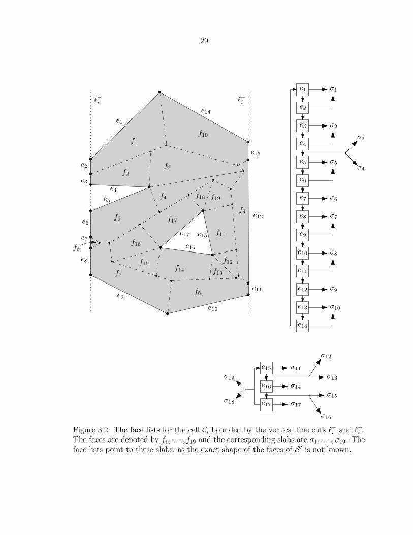
An empty cell is a cell of K(P) whose interior does not overlap with S ′. (See

Figure 3.1a.) Thus an empty cell is entirely contained in a face of S ′. Another type

of cell, called a wedge, will play an important role in the analysis of our algorithm.

Let pq be a ridge of S ′, and let a, b be two points in the interior of pq. Let `a and

`b be the vertical lines through a and b, respectively. Consider the subdivision of P

21

∂P

`∂f

C1

C2

C3C4

C5

(a) The cells C1, . . . , C5 are empty. Thefirst cut is performed along `.

`b

ab

p q

`a

C

(b) The wedge C corresponding to ab.

Figure 3.1: Empty cells and a wedge.

obtained by inserting vertical boundaries along `a and `b, and the four descent paths

from a and b. (See Figure 3.1b.) The cell of this subdivision containing ab is called

the wedge corresponding to ab. The lemma below shows that wedges are the only

cells that can overlap the interior of a ridge, without enclosing any of its endpoints.

Lemma 6. Let Ci be a cell overlapping a ridge, but not its endpoints. Then Ci is a

wedge.

Proof. Let a and b be the points on ∂Ci which are farthest along the ridge in either

direction. A ridge can only meet descent paths that start from it, so a and b must

each lie on a vertical cut, `a and `b. No vertical cut has been made between a and

b, otherwise a and b could not be in the same cell. So there is no vertical cut in the

interior of the wedge corresponding to ab, and thus no descent path has been traced

inside this wedge. It follows that this wedge is Ci.

3.2 Data structure

During the course of the algorithm, we maintain the polygon P and its subdivision

K(P) in a doubly-connected edge list [4]. So each cell Ci is represented by a circular

22

list of edges, or several if it has holes. In the following, we show how we augment

these chains so that they record incidences between the boundary of Ci and the faces

of S ′.

For each cell Ci, let S ′i be the subdivision of Ci induced by S ′. So the faces of S ′iare the connected components of Ci \ S ′. Let Q denote a circular list of edges that

form one component of ∂Ci. We subdivide each vertical edge of Q at each intersection

point with an edge of S ′. Now each edge e of Q bounds exactly one face fj of S ′i.

We store a pointer from e to the slab σj corresponding to fj. In addition, for each

vertex of Q which is a reflex vertex of P , we store pointers to the two corresponding

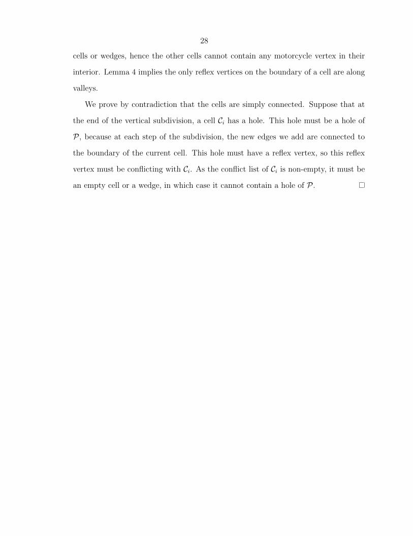
motorcycle slabs. We call this data structure a face list. So we store one face list for

each connected component of ∂Ci. (See Figure 3.2.)

We say that a vertex v of the motorcycle graph G conflicts with a cell Ci of K(P) if

either v lies in the interior of Ci, or v is a reflex vertex of ∂Ci. We also store the list of

all the vertices conflicting with each cell Ci. This list Vi is called the vertex conflict list

of Ci. The size of this list is denoted by vi. In summary, our data structure consists

of:

• A doubly-connected edge list storing K(P).

• The face lists and the vertex conflict list Vi of each cell Ci.

We say that an edge e of S ′ conflicts with the cell Ci if it intersects the interior of

Ci. So any edge of S ′i that is not on ∂Ci is of the form e ∩ Ci for some edge e of S ′

conflicting with Ci. We denote by ci the number of edges conflicting with Ci. During

the course of the algorithm, we do not necessarily know all the edges conflicting with

a cell Ci, and we don’t even know ci, but this quantity will be useful for analysing the

running time. In particular, it allows to bound the size of the data structure for Ci.

Lemma 7. If Ci is non-empty, then the total size of the face lists of Ci is O(ci). In

particular, it implies that ∂Ci has O(ci) edges, and Ci overlaps O(ci) faces of S ′. On

23

the other hand, if Ci is empty, then the total size is O(1), and thus ∂Ci has O(1) edges.

Proof. Let Q denote the outer boundary of Ci, and let |Q| denote its number of edges.

By Lemma 3, each reflex vertex p of Q is in a valley, and the two edges of Q incident

to p bound the two faces of S ′i incident to this valley. So any subchain Q′ of Q that

bounds only one face f ′ of S ′i must be convex. The edges of Q′ can take only 3

directions: vertical, parallel to the base edge of f , or the steepest descent direction.

So Q′ can have at most 5 edges: two vertical edges, two edges parallel to the steepest

descent direction, and one edge along the base edge of f ′.

Thus, Q can be partitioned into at least |Q|/5 subchains, such that two consecutive

subchains bound different faces. Any vertex of Q at which two consecutive subchains

meet must be incident to an edge e of S ′i that conflicts with Ci. By Lemma 4 and 5,

this edge can meet ∂Ci at most twice. So in total, Q has at most 10(ci + 1) edges.

Now consider the holes of Ci, if any. Such a hole must be a hole of P , so each

vertex along its boundary is the endpoint of at least one edge that conflicts with Ci.

Each conflicting edge is adjacent to at most one hole vertex, so there are O(ci) such

vertices in Ci. In addition, each edge of a hole bounds only one face, and for each

reflex vertex, another two faces corresponding to motorcycle slabs are added. So in

total, the face lists for holes have size O(ci).

We just proved that the total size of the face lists is O(ci + 1). If ci is non-empty,

we have ci ≥ 1, and thus the bound can be written O(ci). Otherwise, if Ci is empty,

then it does not conflict with any edge, so ci = 0. Hence, the data structure has size

O(1).

3.3 Algorithm

Our algorithm partitions P recursively, using vertical cuts, as in Sect. 3.1. In this

section, we show how to perform a step of this subdivision in near-linear time. A

24

cell Ci is subdivided along a vertical cut through its median conflicting vertex, so the

vertex conflict lists of the new cells will be at most half the size of the conflict lists of

Ci. When the vertex conflict list of Ci is empty, we call the procedure Divide-Valley

presented in Chapter 4. If Ci is empty or is a wedge, then we we stop subdividing Ci,

and it becomes a leaf cell.

We now describe in more details how we perform this subdivision efficiently. We

assume that the cell Ci conflicts with at least one vertex, and that Ci is given with

the corresponding data structure as described in Sect. 3.2. We first find the median

conflicting vertex in time O(vi). We compute the list of vertical boundary segments

s1, . . . sq created by the cut along the vertical line ` through the median vertex. This

list is sorted along `, and it can be constructed in time proportional to the number

of edges bounding Ci, which is O(ci) by Lemma 7.

Then we compute the lifted polylines s1, . . . , sq as follows. Let H denote the

vertical plane through `. We first find the list of slabs corresponding to the faces of

S ′i. We obtain this list as the union of the slabs that appear in the face lists of Ci.

We compute the intersection of each such slab with H. This gives us a set of O(ci)

segments in H, of which we compute the lower envelope. It can be done in O(ci log ci)

time using an algorithm by Hershberger [19]. Then we obtain s1, . . . , sq by scanning

through this lower envelope and the list s1, . . . , sq. Overall it takes time O(ci log ci) to

compute this lower envelope, and it has O(ci) edges, as each edge of S ′i or Ci creates

at most one vertex along this chain.

The partition induced by ` is obtained by tracing steepest descent paths from

s1, . . . , sq. For each vertical edge sj, and for each edge e of S ′i that meets sj, we do

the following. There are at most three steepest descent paths from a = e ∩ sj, one

for each slab through a. Each such descent path consists of one line segment along

σ, followed possibly by another line segment along a valley if σ is a motorcycle slab.

Let γ denote one of these descent paths. As we know the slab and the starting point

25

of σ, we can construct γ in constant time. This path γ goes all the way to ∂P , so if

necessary, we clip it at `−i or `+i to obtain its restriction to Ci.

These descent paths cannot cross, and by construction they do not cross the

vertical boundary edges. Each edge of S ′i may create at most three such descent

paths, so we create O(ci) such new descent paths. There are also O(ci) new vertical

edges, so we can update the doubly-connected edge list in time O(ci log ci) by plane

sweep. Using an additional O(vi log ci) time, we can update the vertex conflict lists

during this plane sweep. The face lists can be updated in overall O(ci) time by

splitting the face lists of Ci along the lower endpoints of the new descent paths, and

inserting new subchains along each vertical edge sj, which we obtain directly from sj

in linear time. So we just proved the following:

Lemma 8. We can compute the subdivision of a non-empty cell Ci induced by a line

through its median conflicting vertex, and update our data structure accordingly, in

O((ci + vi) log ci) time.

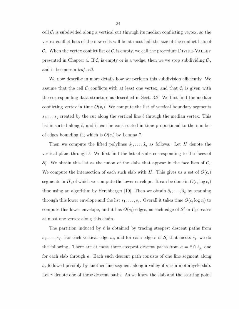
Algorithm 1 Vertical subdivision

1: procedure Divide-Vertical(Ci)2: Select median vertex in Vi, and draw the vertical line ` through it.3: Construct the vertical edges s1, . . . , sq of ` ∩ Ci.4: Compute the lower envelope of the slabs along the vertical plane through `.5: Construct the lifted version s1, . . . , sq of the vertical boundary segments.6: Trace within Ci the steepest descent paths from each vertex of s1, . . . , sq.7: Update K(P) using s1, . . . , sq and the descent paths as new boundaries.8: for each child cell Cj of Ci do9: Construct the data structure for Cj.

10: if Cj is a wedge or is empty then11: Compute S ′j by brute force.12: else13: if Vj = ∅ then14: Call Divide-Valley(Ci)15: else16: Call Divide-Vertical(Cj).

26

3.4 Analysis

In the previous section, we saw that the vertical subdivision of each cell Ci can be

obtained in time near-linear in the size of the data structure for Ci. We now bound

the overall running time of the algorithm, so we need to bound the sum∑

i ci + vi

over all cells created by Divide-Vertical.

We use the recursion tree associated with Algorithm 1. Each node ν of this tree

represents a cell Ci, and the child cells of Ci are stored at the descendants of ν in the

recursion tree. In particular, the cells stored at the descendants of ν form a partition

of the cell stored at ν. Each time we subdivide a cell Ci, the conflict list of each new

cell has at most half the size of the conflict list of Ci. As there are at most 2r vertices

in G, it follows that:

Lemma 9. The recursion tree of Divide-Vertical has depth O(log r).

The degree of any vertex in K(P) is at most 5, because there can be at most three

descent paths through any point, as well as two vertical edges. It implies that any

point of P is contained in at most 5 cells at each level of the recursion tree. It follows

that:

Lemma 10. Any point in P is contained in O(log r) cells of K(P) throughout the

algorithm.

In particular, if we apply this result to each of the 2r vertices of G, we obtain:

Lemma 11. Throughout the algorithm, the sum∑

i vi of the sizes of the vertex con-

flict lists is O(r log r).

We now bound the total number of conflicts between edges of S ′ and cells of K(P).

Lemma 12. Throughout the algorithm, each edge e of S ′ conflicts with O(log r) cells.

It follows that∑

i ci = O(n log r).

27

Proof. Let p, q denote the endpoints of e. First we assume that e is a ridge. By

Lemma 10, there are at most O(log r) cells containing p or q, so it remains to bound

the number of cells that overlap e but not p, q. By Lemma 6, these must be wedges.

There can only be a wedge along e if at least two vertical cuts through e have been

made. When the second such cut is made, the wedge associated with a segment

ab ⊂ e is created. Assume without loss of generality that a is between p and b. Any

wedge is a leaf cell, so in order to create a new wedge along e, one must cut with a

vertical line through pa or bq. (See Figure 3.3.) It creates a new wedge adjacent to

the first one, and it splits the cell containing p or q, creating a new cell containing p

or q. Repeating this process, we can see that for each new wedge created along e, a

new cell containing p or q is created. So there can be only O(log r) wedges along e.

If e is a valley or a flat edge, then by Lemma 4, it only conflicts with cells that

contain its higher endpoint, so throughout the algorithm, there are O(log r) such cells

by Lemma 10.

We can now state the main result of this section. Its proof follows from Lemma 7,

8, Lemma 11, and 12.

Lemma 13. The vertical subdivision procedure completes in O(n(log n) log r) time.

The cells of the resulting subdivision are either empty cells, wedges, or do not contain

any motorcycle vertex in their interior. They are simply connected, and the only reflex

vertices on their boundaries are along valleys.

Proof. When we perform a subdivision, we can identify in constant time each empty

child cell, because by Lemma 7, these cells have constant size. When we find such

a cell, we do not recurse on it, so these cells do not affect the running time of our

algorithm. Therefore, by Lemma 8, the running time of Algorithm 1 is the O(∑

i(ci+

vi) log ci) over all cells created during the course of the algorithm. By Lemma 11 and

12, this quantity is O(n(log n) log r). The only cells that are not subdivided are empty

28

cells or wedges, hence the other cells cannot contain any motorcycle vertex in their

interior. Lemma 4 implies the only reflex vertices on the boundary of a cell are along

valleys.

We prove by contradiction that the cells are simply connected. Suppose that at

the end of the vertical subdivision, a cell Ci has a hole. This hole must be a hole of

P , because at each step of the subdivision, the new edges we add are connected to

the boundary of the current cell. This hole must have a reflex vertex, so this reflex

vertex must be conflicting with Ci. As the conflict list of Ci is non-empty, it must be

an empty cell or a wedge, in which case it cannot contain a hole of P .

29

`+i`−i

e1

e2

e3e4

e5

e6

e7

e8

e9

e10

e11

e12

e13

e14

e17 e15

e16

f1

f2f3

f4

f5

f6

f7

f8

f9

f10

f19

f11

f12

f13f14

f15

f16

f17

f18

e1

e2

e3

e4

e5

e6

e7

e8

e9

e10

e11

e12

e13

e14

σ1

σ2

σ3

σ4σ5

σ6

σ7

σ8

σ9

σ10

e15

e16

e17

σ11

σ14

σ17

σ12

σ13

σ15

σ16

σ18

σ19

Figure 3.2: The face lists for the cell Ci bounded by the vertical line cuts `−i and `+i .The faces are denoted by f1, . . . , f19 and the corresponding slabs are σ1, . . . , σ19. Theface lists point to these slabs, as the exact shape of the faces of S ′ is not known.

30

p

q

a

b

p

q

a

b

Figure 3.3: A first wedge is created (left), and an adjacent wedges is created afterwards(right). The cell containing p has been split simultaneously.

31

(a) Input polygon and straight skeleton. (b) First vertical cut.

(c) Subdivision induced by the first ver-tical cut. (d) Second vertical cut.

(e) Subdivision induced by the secondvertical cut. (f) Third vertical cut.

Figure 3.4: The vertical subdivision. (Continued in Figure 4.2.)

32

Chapter 4

Cutting between valleys

4.1 Algorithm

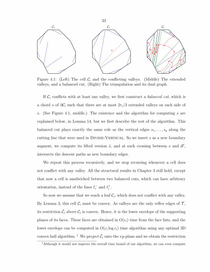
In this section, we describe the second stage of the algorithm. The corresponding

procedure is called Divide-Valley, and its pseudocode is supplied in Algorithm 2.

Let Ci be a cell of K(P) constructed by Divide-Vertical on which we call Divide-

Valley. This cell Ci is not empty and is not a wedge, as they are handled by brute

force by Divide-Vertical, so by Lemma 13, it does not contain any reflex vertex

in its interior. Let Ri denote the set of valleys that conflict with Ci, and let ri denote

its cardinality. The extended valley e′ corresponding to a valley e ∈ Ri is the segment

obtained by extending e until it meets the boundary ∂Ci of the cell. By Lemma 4, the

valley e must meet ∂Ci, so we only need to extend it in one direction so as to obtain

e′. As Ci does not contain any motorcycle vertex in its interior, it implies that the

extended valleys of Ci do not cross. By Lemma 4, the cell Ci is simply connected, so

the extended valleys form an outerplanar graph with outer face ∂Ci. (See Figure 4.1.)

At this stage of the algorithm, the cells are simply connected, so we record each

cell Ci using a single face list. We do not need vertex conflict lists, as the cells do not

conflict with any vertex. We do not need to store the valley conflict list Ri either, as

we can obtain it in linear time from the face list.

33

CiCi

s

Ci

Figure 4.1: (Left) The cell Ci and the conflicting valleys. (Middle) The extendedvalleys, and a balanced cut. (Right) The triangulation and its dual graph.

If Ci conflicts with at least one valley, we first construct a balanced cut, which is

a chord s of ∂Ci such that there are at most 2ri/3 extended valleys on each side of

s. (See Figure 4.1, middle.) The existence and the algorithm for computing s are

explained below, in Lemma 14, but we first describe the rest of the algorithm. This

balanced cut plays exactly the same role as the vertical edges s1, . . . , sq along the

cutting line that were used in Divide-Vertical. So we insert s as a new boundary

segment, we compute its lifted version s, and at each crossing between s and S ′,

intersects the descent paths as new boundary edges.

We repeat this process recursively, and we stop recursing whenever a cell does

not conflict with any valley. All the structural results in Chapter 3 still hold, except

that now a cell is sandwiched between two balanced cuts, which can have arbitrary

orientation, instead of the lines `−i and `+i .

So now we assume that we reach a leaf Ci, which does not conflict with any valley.

By Lemma 3, this cell Ci must be convex. As valleys are the only reflex edges of T ,

its restriction Ci above Ci is convex. Hence, it is the lower envelope of the supporting

planes of its faces. These faces are obtained in O(ci) time from the face lists, and the

lower envelope can be computed in O(ci log ci) time algorithm using any optimal 3D

convex hull algorithm. 1 We project Ci onto the xy-plane and we obtain the restriction

1Although it would not improve the overall time bound of our algorithm, we can even compute

34

S ′i of S ′ to Ci.

Algorithm 2 Cutting between valleys

1: procedure Divide-Valley(Ci)2: if no valley conflicts with Ci then3: Compute S ′ ∩ Ci as a lower envelope of planes.4: return5: Build the list of all valleys conflicting with Ci.6: Construct a balanced cut s as in Lemma 14.7: Construct the vertical slab H through s.8: Construct s as the lower envelope of the slabs intersecting H.9: Trace within Ci the two or three steepest descent paths from each vertex of s.

10: Update the partition K(P) using s and the descent paths as new boundaries.11: for each child cell Cj of Ci do12: Construct the data-structure for Cj.13: Call Divide-Valley(Cj).

4.2 Analysis

It remains to analyse this algorithm, and prove the existence of a balanced cut.

Lemma 14. Given a simply connected cell Ci that does not conflict with any motor-

cycle vertex, and that conflicts with at least one valley, and given the face list of Ci,

we can compute a balanced cut of Ci in time O(ci log ci).

Proof. By Lemma 7, the cell Ci has O(ci) edges. We obtain the list Ri of valleys

conflicting with Ci in O(ci) time by traversing the face list. Let e1, . . . , eq denote

these valleys. We first compute the set of extended valleys R′i = e′1, . . . , e′q. The set

R′i can be obtained in O(ci) time by traversing ∂Ci. We start at an arbitrary vertex

of Ci, and each time we encounter the lower endpoint of a valley, we push the valley

into a stack. At each edge u of Ci that we traverse, we check whether the extended

Ci in O(ci) time using a linear-time algorithm for the medial axis of a convex polygon [1]: Firstconstruct the polygon on the xy-plane that is bounded by the traces of the supporting planes of thefaces of Ci, then compute its medial axis, and construct its intersection with Ci.

35

valley e′j at the top of the stack meets it, and if so, we draw e′j, we pop it out of the

stack, and we check whether the new edge at the top of the stack meets u.

Now we consider the outerplanar graph obtained by inserting the chords of R′i

along ∂Ci. (See Figure 4.1, middle.) We triangulate this graph, which can be done in

O(ci) time using Chazelle’s linear-time triangulation algorithm [5], or in O(ci log ci)

time using simpler algorithms [4]. We construct the dual of this triangulation. We

subdivide any edge of the dual corresponding to an extended valley, and we assign

weight one to the new node. The other nodes have weight zero. This graph is a tree,

with degree at most 3, so we can compute a weighted centroid ω in time O(ci) [21].

This centroid is a node of the tree such that each connected component of the forest

obtained by removing the centroid has weight at most ri2

.

If ω corresponds to an extended valley e′j, we pick s = e′j as the balanced cut. It

splits Ri into two subsets of size at most ri2

. Otherwise, ω corresponds to a face of the

triangulation, such that the three subgraph rooted at c have weight at most ri2

. We

cut along the edge s of this triangular face corresponding to the subtree with largest

weight.

Lemma 14 plays the same role as Lemma 8 in the analysis of Divide-Vertical.

At each level of recursion, the size of the largest conflict list Ri is multiplied by at

most 23, so the recursion depth is still O(log r). A leaf cell Ci is handled in O(ci log ci)

time by computing a lower envelope of planes, as explained above. It follows that we

can complete the second step of the subdivision, and compute S ′ within each cell, in

overall O(n(log n) log r) time. Then Theorem 1 follows.

Our analysis of this algorithm is tight, as shown by the example in Section 5.2.

36

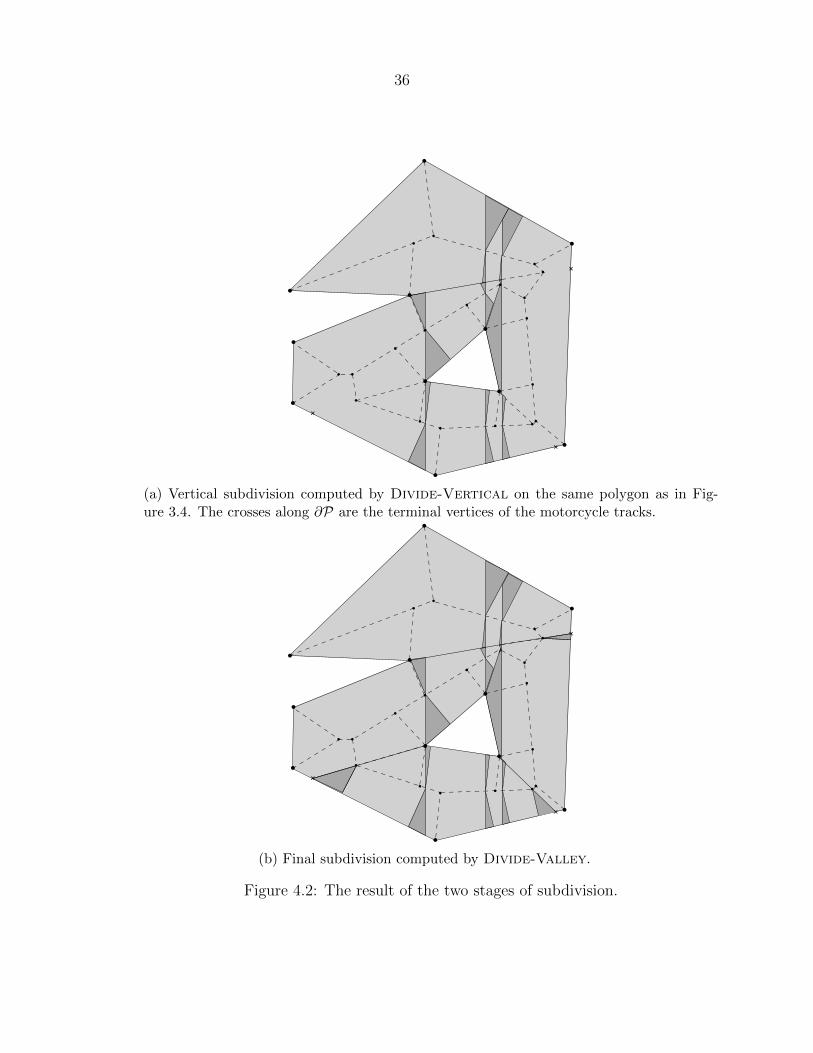
(a) Vertical subdivision computed by Divide-Vertical on the same polygon as in Fig-ure 3.4. The crosses along ∂P are the terminal vertices of the motorcycle tracks.

(b) Final subdivision computed by Divide-Valley.

Figure 4.2: The result of the two stages of subdivision.

37

Chapter 5

Summary

We accomplished our objectives of developing a new algorithm for solving the Straight

Skeleton Problem and proving rigorously that it is asymptotically faster than all

previous algorithms. The current bound of O(n log r log n + r4/3+ε) time for a non-

degenerate polygon is a strict improvement over the previous bound ofO(n√h+ 1 log2 n+

r4/3+ε) expected time. Details on generalisations and comparisons of this result are

described in Table 1.1.

Our algorithm is deterministic, and arguably simpler to understand and implement

than several other fast algorithms. The main data structures required are the doubly-

connected edge list [4] and face lists (see Section 3.2)

5.1 Degenerate cases

As discussed in Chapter 2, the description and analysis of our algorithm was given

for polygons in general position. Here we briefly explain why our result generalises

to arbitrary polygons.

As explained in the article by Eppstein and Erickson [15], almost all degeneracies

can be treated by standard perturbation techniques, replacing high degree nodes with

several nodes of degree 3. The only difficult case is when two or more valleys meet, and

generate a new valley. In the induced motorcycle graph, this situation is represented

38

by two or more motorcycle colliding, and generating a new motorcycle [18].

So in degenerate cases, we assume that the exact induced motorcycle graph has

been computed. It can be done in time O(r17/11+ε) for any ε > 0, using Eppstein

and Erickson’s algorithm [15]. Then the problem becomes a problem of computing a

lower envelope of slabs. Standard perturbation techniques apply to this problem [14],

so our non-degeneracy assumptions are valid.

The only difference with the non-degenerate case is that now, instead of having

each valley adjacent to a reflex vertex, the valleys form a forest, with leaves at the

reflex vertex. So a descent path may be a polyline with arbitrarily many vertices.

Thus, when we perform a vertical cut, we cannot necessarily trace a descent path

in constant time. However, we can trace it in time proportional to its size, and its

edges become cell boundaries. The subdivision can be updated in amortised O(log n)

time for each such edge, as we update the partition by plane sweep. So the extra

contribution to the overall running time is O(n log n).

5.2 Tightness of analysis

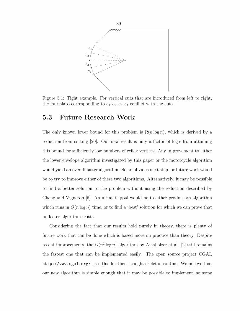
We give an example to demonstrate that for this algorithm the analysis is tight.

Consider a polygon P where, on the left hand side, we have a convex chain of Ω(n)

near-vertical edges. Along the top boundary of P we have Ω(r) small reflex dips

pointing downwards. See Figure 5.1 for an example with a convex chain of size 4, and

5 reflex dips. The straight skeleton faces corresponding to each edge of the convex

chain to the left of the polygon extend deep into the polygon. Each time we make

a vertical cut to the right of all other vertical cuts previously made, it will cross

through all faces of the chain, hence all the slabs must be provided to the lower

envelope calculation. It then follows that Algorithm 1 spends Ω(n(log n) log r) time

as it computes Ω(log r) lower envelopes of size Ω(n).

39

e1

e2

e3

e4

Figure 5.1: Tight example. For vertical cuts that are introduced from left to right,the four slabs corresponding to e1, e2, e3, e4 conflict with the cuts.

5.3 Future Research Work

The only known lower bound for this problem is Ω(n log n), which is derived by a

reduction from sorting [20]. Our new result is only a factor of log r from attaining

this bound for sufficiently low numbers of reflex vertices. Any improvement to either

the lower envelope algorithm investigated by this paper or the motorcycle algorithm

would yield an overall faster algorithm. So an obvious next step for future work would

be to try to improve either of these two algorithms. Alternatively, it may be possible

to find a better solution to the problem without using the reduction described by

Cheng and Vigneron [6]. An ultimate goal would be to either produce an algorithm

which runs in O(n log n) time, or to find a ‘best’ solution for which we can prove that

no faster algorithm exists.

Considering the fact that our results hold purely in theory, there is plenty of

future work that can be done which is based more on practice than theory. Despite

recent improvements, the O(n2 log n) algorithm by Aichholzer et al. [2] still remains

the fastest one that can be implemented easily. The open source project CGAL

http://www.cgal.org/ uses this for their straight skeleton routine. We believe that

our new algorithm is simple enough that it may be possible to implement, so some

40

benchmark testing would be of great interest. The use of the divide and conquer

paradigm also opens up the possibility for efficient parallelisation.

41

REFERENCES

[1] A. Aggarwal, L. J. Guibas, J. Saxe, and P. W. Shor. A linear-time algorithm for

computing the voronoi diagram of a convex polygon. Discrete and Computational

Geometry, 4(1):591–604, 1989.

[2] O. Aichholzer, D. Alberts, F. Aurenhammer, and B. Gartner. A novel type of

skeleton for polygons. Journal of Universal Computer Science, 1(12):752–761,

1995.

[3] G. Barequet, M. Goodrich, A. Levi-Steiner, and D. Steiner. Straight-skeleton

based contour interpolation. Proceedings of the 14th annual ACM-SIAM sympo-

sium on Discrete algorithms, pages 119–127, 2003.

[4] Mark de Berg, Otfried Cheong, Marc van Kreveld, and Mark Overmars. Com-

putational Geometry: Algorithms and Applications. Springer-Verlag, 2008.

[5] B. Chazelle. Triangulating a simple polygon in linear time. Discrete Comput.

Geom., 6(5):485–524, August 1991.

[6] S.-W. Cheng and A. Vigneron. Motorcycle graphs and straight skeletons. Algo-

rithmica, 47(2):159–182, 2007.

[7] F. Chin, J. Snoeyink, and C. A. Wang. Finding the medial axis of a simple

polygon in linear time. Discrete and Computational Geometry, 21(3):405–420,

1999.

[8] F. Cloppet, J. Oliva, and G. Stamon. Angular bisector network, a simplified

generalized voronoi diagram: Application to processing complex intersections

in biomedical images. IEEE Transactions on Pattern Analysis and Machine

Intelligence, 22(1):120–128, 2000.

[9] S. Coquillart, J. Oliva, and M. Perrin. 3d reconstruction of complex polyhedral

shapes from contours using a simplified generalized voronoi diagram. Computer

Graphics Forum, 15(3):397–408, 1996.

42

[10] A. Day and R. Laycock. Automatically generating large urban environments

based on the footprint data of buildings. Proceedings of the 8th ACM symposium

on Solid Modeling and Applications, pages 346–351, 2003.

[11] E. D. Demaine, M. L. Demaine, and A. Lubiw. Folding and cutting paper.

Revised Papers from the Japan Conference on Discrete and Computational Ge-

ometry, pages 104–117, 1998.

[12] E. D. Demaine, M. L. Demaine, and A. Lubiw. Folding and one straight cut

suffice. Proceedings of the 10th Annual ACM-SIAM Symposium on Discrete

Algorithms, pages 891–892, 1999.

[13] E. D. Demaine, M. L. Demaine, and J. S. B. Mitchell. Folding flat silhouettes and

wrapping polyhedral packages: New results in computational origami. Proceed-

ings of the 15th Annual ACM Symposium on Computational Geometry, pages

105–114, 1999.

[14] H. Edelsbrunner and E. P. Mucke. Simulation of simplicity: A technique to cope

with degenerate cases in geometric algorithms. ACM Trans. Graph., 9(1):66–104,

1990.

[15] D. Eppstein and J. Erickson. Raising roofs, crashing cycles, and playing pool:

Applications of a data structure for finding pairwise interactions. Discrete and

Computational Geometry, 22(4):569–592, 1999.

[16] P. Felkel and S. Obdrzalek. Straight skeleton implementation. Proceedings of the

14th Spring Conference on Computer Graphics, pages 210–218, 1998.

[17] M. Held and S. Huber. Theoretical and practical results on straight skeletons of

planar straight-line graphs. Proceedings of the 27th Symposium on Computational

Geometry, pages 171–178, 2011.

[18] M. Held and S. Huber. A fast straight-skeleton algorithm based on general-

ized motorcycle graphs. International Journal of Computational Geometry and

Applications, 22(5):471–498, 2012.

[19] J. Hershberger. Finding the upper envelope of n line segments in O(n log n)

time. Information Processing Letters, 33(4):169–174, 1989.

[20] S. Huber. Computing Straight Skeletons and Motorcycle Graphs: Theory and

Practice. PhD thesis, University of Salzburg, Austria, 2011.

43

[21] O. Kariv and S. Hakimi. An algorithmic approach to network location problems.

II: The p-medians. SIAM Journal on Applied Mathematics, 37(3):539–560, 1979.

[22] T. Kelly and P. Wonka. Interactive architectural modeling with procedural ex-

trusions. ACM Transactions on Graphics, 30(2):14:1–14:15, 2011.

[23] A. Vigneron and L. Yan. A faster algorithm for computing motorcycle graphs.

Proceedings of the 29th Symposium on Computational Geometry, pages 17–26,

2013.

[24] G. von Peschka. Kotirte Ebenen: Kotirte Projektionen und deren Anwendung;

Vortrage. Brno: Buschak and Irrgang, 1877.

44

6 Papers Submitted

• Siu-Wing Cheng, Liam Mencel, and Antoine Vigneron, “A Faster Algorithm for

Computing Straight Skeletons”, Submitted to the 22nd European Symposium on Al-

gorithms, 2014.