a faithful semantics for generalised … · generalised symbolic trajectory ... meaning that...

Logical Methods in Computer ScienceVol. 5 (2:1) 2009, pp. 1–32www.lmcs-online.org

Submitted Jun. 7, 2007Published Apr. 8, 2009

A FAITHFUL SEMANTICS FOR

GENERALISED SYMBOLIC TRAJECTORY EVALUATION

KOEN CLAESSEN a AND JAN-WILLEM ROORDA b

a Chalmers University of Technology, Swedene-mail address: [email protected]

b Fenix Design Automation, the Netherlandse-mail address: [email protected]

Abstract. Generalised Symbolic Trajectory Evaluation (GSTE) is a high-capacity for-mal verification technique for hardware. GSTE is an extension of Symbolic TrajectoryEvaluation (STE). The difference is that STE is limited to properties ranging over finitetime-intervals whereas GSTE can deal with properties over unbounded time.

GSTE uses abstraction, meaning that details of the circuit behaviour are removed fromthe circuit model. This improves the capacity of the method, but has as down-side thatcertain properties cannot be proven if the wrong abstraction is chosen.

A semantics for GSTE can be used to predict and understand why certain circuitproperties can or cannot be proven by GSTE. Several semantics have been described forGSTE by Yang and Seger. These semantics, however, are not faithful to the provingpower of GSTE-algorithms, that is, the GSTE-algorithms are incomplete with respect tothe semantics. The reason is that these semantics do not capture the abstraction used inGSTE precisely.

The abstraction used in GSTE makes it hard to understand why a specific propertycan, or cannot, be proven by GSTE. The semantics mentioned above cannot help the userin doing so. So, in the current situation, users of GSTE often have to revert to the GSTEalgorithm to understand why a property can or cannot be proven by GSTE.

The contribution of this paper is a faithful semantics for GSTE. That is, we give a simpleformal theory that deems a property to be true if-and-only-if the property can be provenby a GSTE-model checker. We prove that the GSTE algorithm is sound and completewith respect to this semantics. Furthermore, we show that our semantics for GSTE is ageneralisation of the semantics for STE and give a number of additional properties relatingthe two semantics.

1998 ACM Subject Classification: B.6.3, F.3.2, F.4.3.Key words and phrases: Formal Verification, Formal Specification, Model Checking, Symbolic Simulation,

Generalized Symbolic Trajectory Evaluation, Semantics.lsuper bThis work was carried out while employed at Chalmers University.

LOGICAL METHODSl IN COMPUTER SCIENCE DOI:10.2168/LMCS-5 (2:1) 2009

c© K. Claessen and J.-W. RoordaCC© Creative Commons

http://creativecommons.org/about/licenses

2 K. CLAESSEN AND J.-W. ROORDA

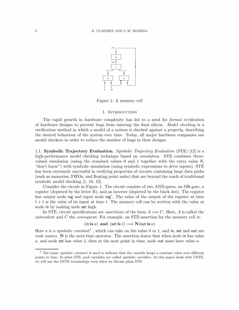
Figure 1: A memory cell

1. Introduction

The rapid growth in hardware complexity has led to a need for formal verification

of hardware designs to prevent bugs from entering the final silicon. Model checking is averification method in which a model of a system is checked against a property, describingthe desired behaviour of the system over time. Today, all major hardware companies usemodel checkers in order to reduce the number of bugs in their designs.

1.1. Symbolic Trajectory Evaluation. Symbolic Trajectory Evaluation (STE) [12] is ahigh-performance model checking technique based on simulation. STE combines three-valued simulation (using the standard values 0 and 1 together with the extra value X,“don’t know”) with symbolic simulation (using symbolic expressions to drive inputs). STEhas been extremely successful in verifying properties of circuits containing large data paths(such as memories, FIFOs, and floating point units) that are beyond the reach of traditionalsymbolic model checking [1, 10, 12].

Consider the circuit in Figure 1. The circuit consists of two AND-gates, an OR-gate, aregister (depicted by the letter R), and an inverter (depicted by the black dot). The registerhas output node reg and input node reg′. The value of the output of the register at timet+ 1 is the value of its input at time t. The memory cell can be written with the value atnode in by making node set high.

In STE, circuit specifications are assertions of the form A =⇒ C. Here, A is called theantecedent and C the consequent. For example, an STE-assertion for the memory cell is:

(in is a) and (set is 1) =⇒ N(out is a)

Here a is a symbolic constant1 , which can take on the value 0 or 1, and in, set and out arenode names. N is the next-time operator. The assertion states that when node in has valuea, and node set has value 1, then at the next point in time, node out must have value a.

1 The name symbolic constant is used to indicate that the variable keeps a constant value over differentpoints in time. In plain STE, such variables are called symbolic variables. As this paper deals with GSTE,we will use the GSTE terminology even when we discuss plain STE.

A FAITHFUL SEMANTICS FOR GENERALISED SYMBOLIC TRAJECTORY EVALUATION 3

1.2. Generalised Symbolic Trajectory Evaluation. One of the main disadvantages ofSTE is that it can only deal with properties ranging over a finite number of time-steps.Generalised Symbolic Trajectory Evaluation (GSTE) [16, 15, 18, 17] is an extension of STEthat can deal with properties ranging over unbounded time.

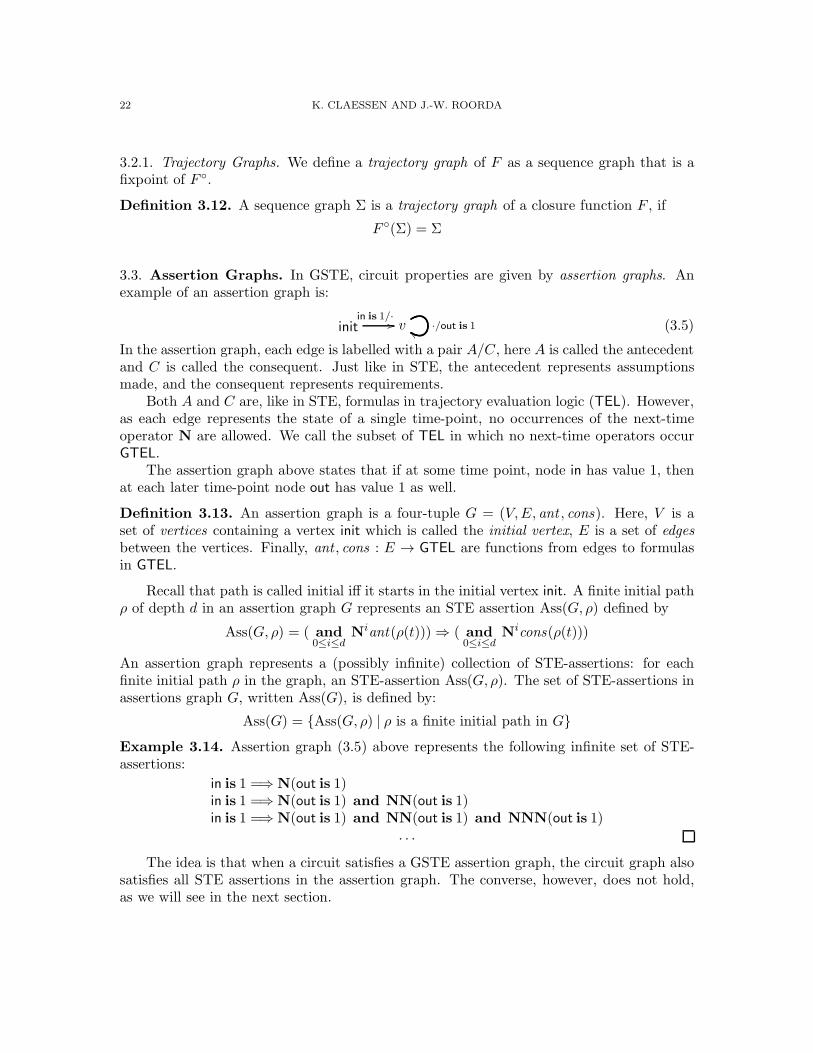
In GSTE, circuit properties are given by assertion graphs. For example, an assertiongraph for the memory cell is:

init(in is a) and (set is 1)/·

// v

set is 0/·

��

·/out is a// w ff (1.1)

In the assertion graph, each edge is labelled with a pair A/C. As in STE, A is called theantecedent and C is called the consequent. The syntax of A and C is like the syntax ofthe antecedent and consequent in STE without the next-time operator N. The N operatorcan not be used because each edge only represents a single time-point. A dot (·) means anempty antecedent or consequent.

The assertion graph above states that if we write value a to the memory cell, and thenfor arbitrary many time-steps we do not write, the memory cell still contains value a.

Each finite path, starting in the initial vertex init of the graph, represents an STEproperty. For instance, the finite paths through the assertion graph above represent thefollowing STE properties:

(in is a) and (set is 1) =⇒ N(out is a)(in is a) and (set is 1) and N(set is 0) =⇒ NN(out is a)(in is a) and (set is 1) and N(set is 0) and NN(set is 0) =⇒ NNN(out is a). . .

Each of these assertions can be proven by an STE model checker. But, as the set ofassertions is infinite, we cannot use plain STE to prove all of them. However, if we useGSTE to prove that the circuit satisfies the above assertion graph, it follows that all STE-assertions represented by the assertion graph hold as well.

Note that in GSTE, just like in STE, the initial values of registers are ignored.

1.3. Earlier work on semantics for GSTE. A semantics for GSTE can be used topredict and understand why certain circuit properties can or cannot be proven by GSTE.In [17, 18] three semantics for GSTE are distinguished: (1) the strong semantics, (2) thenormal semantics, and (3) the fair semantics. The semantics have in common that a circuitssatisfies an assertion-graph if it satisfies all appropriate paths in the assertion graph. Themeaning of appropriate differs over the three semantics, as we explain in the followingparagraphs. As in [5], we refer to this class of semantics as the ∀-semantics, because thesesemantics really consider all concrete paths, rather than approximating this quantificationby applying abstraction.

In the strong semantics, a circuit satisfies a GSTE assertion graph if-and-only-if thecircuit satisfies all STE-assertions corresponding to finite paths in the assertion graph. Forinstance, as the memory cell satisfies the set of finite assertions above, it also satisfiesassertion graph (1.1).

Consider the following assertion graph:

init(set is 1)/(in is a)

// vout is a/·

// w ff (1.2)


Intuitively, we might want the above assertion graph to state that if at some time-pointnode out has value a, and just before that, node set was high, then at this time-point nodein should have value a. This is an example of a backwards property, that is, a property inwhich a consequent depends on an antecedent at a later time-point.

The strong semantics cannot deal with such backwards properties. For instance, forthe above property, the path starting in vertex init and ending in vertex v corresponds tothe assertion

(set is 1) =⇒ (in is a)

This assertion is, of course, not true for the memory cell. But, any run of the circuit thatmakes in is a fail, makes N(out is a) fail as well. So, intuitively, the assertion is not satisfiedbecause a consequent failed before the antecedent it depended on could fail.

In the normal semantics, a circuit satisfies a GSTE assertion graph if-and-only-if thecircuit satisfies the STE-assertions corresponding to all infinite paths in the assertion graph.Therefore, the normal semantics can deal with backwards properties as well. For instance, inassertion graph (1.2), there is only one infinite path. This path corresponds to the followingassertion:

(set is 1) and N(out is a) =⇒ (in is a)

As any circuit trace that satisfies the antecedent satisfies the consequent as well, this asser-tion is satisfied by the circuit. Thus, in the normal semantics, the GSTE assertion graph issatisfied.

Finally, the need for the fair semantics is illustrated by the following example. Considerthe assertion graph:

init(set is 1)/(in is a)

// v

set is 0/·

��

out is a/·// w ff (1.3)

The assertion graph above states that if at some time-point node out has value a, and beforethat, for a period of time no values were written to the memory-cell, and before that, setwas high, then at this time-point in should have value a.

In the normal semantics, the memory cell circuit does not satisfy this assertion graph.Consider the infinite path starting in init and then cycling at the self-loop at v for ever.This path corresponds to the infinite assertion:

(set is 1) and N(set is 0) and NN(set is 0) and . . . =⇒ in is a

For a given a, this assertion can be falsified by the trace in which value ¬a is written attime 0, and is kept in memory since then.

In the fair semantics for GSTE, this problem is solved by selecting a set of fair edges.The semantics only considers paths that visit every fair edge infinitely often. For instance,if in the above assertion graph the edge from vertex w to itself is made fair, the assertiongraph holds in the fair semantics.

1.4. GSTE model checking. In the same papers [17, 18], model checking algorithms fornormal, strong and fair GSTE are described. It is proven that the model checking algorithmsare sound with respect to their corresponding semantics. However, the algorithms are notcomplete. The reason is that the ∀-semantics do not precisely capture the information lossdue to the three-valued abstraction in GSTE.


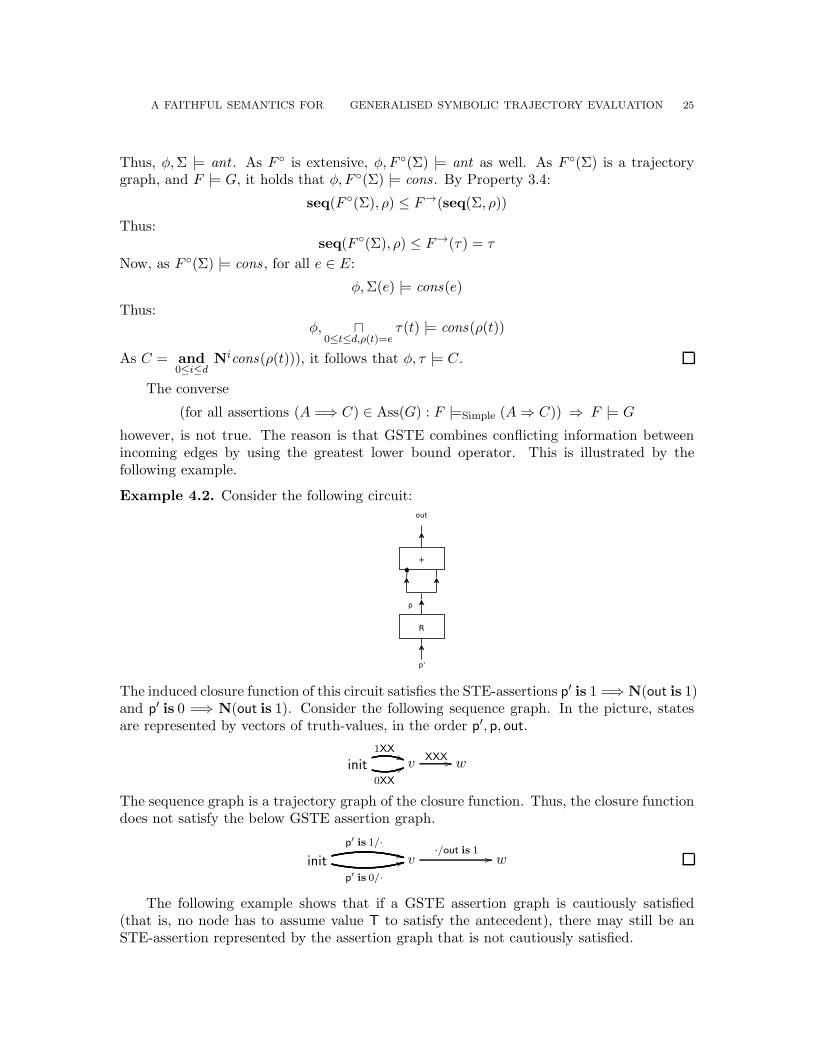
For example, consider the following circuit

and the following assertion graph

init

p′ is 1/·++

p′ is 0/·

33 v·/out is 1

// w ff

The assertion graph represents the following STE-assertions:

p′ is 1 =⇒ N(out is 1)p′ is 0 =⇒ N(out is 1)

Both assertions hold. So, the semantics described above predict that the circuit satisfiesthe assertion graph.

However, it turns out that the GSTE-algorithm cannot prove the assertion graph! Thereason is that GSTE algorithms only compute one three-valued assertion for each edge inthe assertion graph. This is in general not enough to take account for all STE assertionscorresponding to all paths through the assertion graph, so a certain information loss hap-pens. In this particular case, the state calculated on the edge from v to w gives value X

to node out. This can be explained as follows. The antecedent at the top edge betweenvertices init and v requires node p′ to have value 1. The antecedent at the bottom edgerequires node p′ to have value 0. Node p′ is the input to a register with node p as output.So, when the edge from v to w is reached via the top edge between init and v node p willreceive value 1. When the edge from v to w is reached via the bottom edge between init

and v, node p will receive value 0. As the value of node p should comply with both paths,the algorithm chooses value X for node p, and thus node out receives value X as well.

1.5. The problem. The previous example illustrates that the ∀-semantics for GSTE dis-cussed previously cannot be used to explain how the three-valued abstraction causes certainproperties to be not provable with GSTE. This can lead to situations where seemingly trivialchanges to either the circuit or the assertion can suddenly make an assertion not provableanymore.

This is an undesirable situation. We believe that a faithful semantics for GSTE isneeded.

A faithful semantics deems a property to be true if-and-only-if the property can beproven by a GSTE-model checker. Without a faithful semantics, a GSTE verification engi-neer is left to the particular internals of the model checker at hand to understand what canand cannot be proved. Also, a faithful semantics can be used to understand differences be-tween different GSTE model checkers. For example, the GSTE semantics of satGSTE [14]


is expressed using successive unrollings of the assertion graph as STE assertions. However,the abstraction obtained in that way does not correspond to the abstraction in standardGSTE model checkers. This means that there are assertion graphs for which satGSTE andstandard GSTE model checkers give different answers.

To further clarify the importance of a faithful GSTE semantics, we would like to pointout that there is a difference between the use of abstraction in (G)STE, and the applicationof abstraction as a performance enhancer in model checkers for standard temporal logicslike LTL and CTL. In the latter case, a model checker might simply give up when it happensto choose an abstraction that is too weak to prove a property, but it is still clear to theverification engineer what the specification means. In (G)STE, what abstraction to use inthe model checker is an artefact of the specification, not an artefact of the model checker. So,in (G)STE it is vital to understand what a specification means, separate from a particularmodel checker, including the abstraction that is specified.

In previous work [9], we have described a faithful semantics for STE. However, up tillnow, no faithful semantics for GSTE has been described.

1.6. Our contribution. In this paper, we present a semantics for GSTE that is faithfulto the proving power of the GSTE model checking algorithm. Compared to the semanticsdescribed in [17, 18], our semantics corresponds to the strong semantics of GSTE. That is, inthis paper, we do not consider backwards properties or fairness constraints, which remainsfuture work. One difference with the strong semantics in [17, 18] is that our semanticscaptures the three-valued abstraction of GSTE precisely, and thus can be used to explainthe information loss caused by the three-valued abstraction in GSTE.

Another difference is that our semantics for GSTE follows the same structure as thesemantics for STE [9, 12, 6]. For instance, where STE deals with sequences to representabstract circuit behaviour, our GSTE semantics uses sequence graphs. Here, a sequencegraph is a mapping from edges in an assertion graph to abstract circuit states. We showthat our GSTE semantics is a generalisation of the STE semantics. That is, given a linearassertion graph, the STE-semantics and GSTE-semantics are equivalent. Finally, we statea number of additional properties relating the two semantics.

We believe that our faithful semantics for STE is an important contribution to theresearch on GSTE for at least two reasons.

First of all, a faithful semantics makes GSTE more accessible to novice users: a faithfulsemantics enables users to understand the abstraction used in GSTE, without having tounderstand the details of the model checking algorithm. Additionally, in this paper, we aimat increasing the understanding for GSTE users of subtle cases of information-loss due toabstraction by providing enlightening examples.

Furthermore, a faithful semantics for GSTE can be used as basis for research on newGSTE model checking algorithms and other GSTE tools. To illustrate this, in previouswork [8], we described a new SAT-based model checking algorithm for STE and proventhat it is sound and complete with respect to our faithful semantics for STE presentedin [9]. Without a faithful semantics for STE, we would have been forced to prove thecorrectness of our algorithm by relating it to other model checking algorithms for STE.This is clearly a more involved and less elegant approach. In fact, we believe that withoutconstructing a faithful semantics for STE first, we would not have obtained the level ofunderstanding of STE needed to develop the new SAT-based model checking algorithm.


In the same way, we expect that the faithful semantics for GSTE presented in thispaper will open the door for new research on GSTE model checking algorithms and otherGSTE tools.

1.7. Other related work. The following papers are based on the ∀-semantics for GSTE.

GSTE as partitioned model checking. In [11], the relation between GSTE and classic sym-bolic model checking is studied. It is explained how GSTE can be seen as a partitioned formof classic symbolic model checking. However, the abstraction of GSTE is not taken intoaccount. Therefore, this paper, focussing on the abstraction in GSTE, is complementary to[11].

Using SAT for debugging of GSTE assertion graphs. In [14], the tool satGSTE is presented.The tool considers a finite subset of all finite paths in an assertion graphs, for instance, allpaths up to a certain length. For each path in this subset, the tool model checks thecorresponding STE assertion. The authors explain how the tool can be used to debug andrefine GSTE assertion graphs. However, their tool does not follow the same semantics asstandard GSTE model checking algorithms. Thus, certain counter examples that wouldoccur in a standard GSTE model checker due to the use of abstraction cannot be foundwith their algorithm.

Monitor circuits for GSTE assertion graphs. In (conventional, non-symbolic) simulation,a model of a circuit is fed with a large number of inputs. For every input it is checkedwhether the output is as expected. Typically, a monitor circuit is used to make this check.The monitor circuit observes the system under verification without interfering. During eachstep of the simulation, it indicates whether the system has obeyed the formal specificationthus far.

In [4, 7] methods for automatic construction of monitor circuits for GSTE assertiongraphs are described. The method in [4] requires the use of a symbolic simulator if theassertion graph contains symbolic constants. In [7] it is explained how, for the class ofso-called simulation friendly assertion graphs, the method of [4] can be extended to dealwith symbolic constants even in conventional non-symbolic simulation.

The papers explain how monitor circuits can be used to make a bridge between GSTEmodel checking and conventional simulation. For instance, monitor circuits can be used toquickly debug and refine GSTE specifications before trying to use more labour intensiveGSTE model checking.

Reasoning about GSTE assertion graphs. Using the construction of monitor circuits forGSTE assertion graphs, [5] describes two algorithms that can be used in compositionalverification using GSTE. The first algorithm decides whether one assertion graph impliesanother. The second algorithm can be used to model check an assertion graph under theassumption that another assertion graph is true.


1.7.1. Relation to this paper. Each of the papers above is based on the ∀-semantics forGSTE. As explained above, the ∀-semantics are not faithful to the proving power of theGSTE model checking algorithms. So, it can occur that a tool described in the papers deemsa GSTE assertion to be true, while the GSTE model checking algorithm cannot prove it.

For instance, the monitor circuits described above cannot be used to debug and refineassertions graphs that are true in the ∀-semantics but yield a spurious counter-examplewhen trying to prove them with a GSTE model checker. The satGSTE tool is limited inthe same way. We elaborate further on this in the future work section of this paper.

1.8. Structure of this paper. In the next section, we revisit the semantics of STE asser-tions. Then, in Section 3, we present our semantics of GSTE assertion graphs. In Section 4,we compare the STE semantics with the GSTE semantics by giving a number of propertiesdescribing their relation. In Section 5, we describe the GSTE model checking algorithmand show that it is sound and complete with respect to our semantics. Finally, in Section6, we conclude and give suggestions for future work.

2. STE Preliminaries

A semantics for STE was first described by Seger and Bryant [12]. Later, a simplifiedand easier to understand semantics was given by Melham and Jones [6]. Both of thesesemantics are expressed in terms of a next state function, expressing the relationship betweentwo consecutive states in the circuit. Unfortunately, neither of these semantics matches theproving power of currently available STE model checkers. The problem is that they cannotdeal with combinational properties (properties ranging over one single point in time). Allsuch properties are deemed to be false by the semantics. Therefore standard next statesemantics does not seem to be a good starting point for finding a faithful semantics forGSTE.

In previous work [9], we have described an alternative semantics for STE that actuallyis faithful to the proving power of STE model checkers. The semantics is called the closure

semantics. Informally, the closure semantics only differs from the traditional STE semanticsfor combinational properties.

A main ingredient of the closure semantics for STE is the concept of a closure function.The idea is that a closure function takes as input a state of the circuit, and calculatesall information about the circuit state at the same point in time that can be derived bypropagating the information in the input state in a forwards fashion. In the next section,we give an alternative semantics for GSTE also based on closure functions.

In this section we briefly describe the closure semantics for STE. For more examplesand a discussion on the differences with the semantics given in [12, 6], we refer the readerto [9].

Readers familiar with [9] can skip most of this section; compared to [9] we slightlychanged notation in the definition of the closure function on sequences, and we introduced anextra variant of a closure semantics called the simple semantics. Furthermore, we adaptedthe terminology to GSTE: we call the variables in STE-assertions symbolic constants toindicate that they keep a constant value over time. Finally, we use finite sequences torepresent circuit behaviour, as opposed to the standard use of infinite sequences. Noticethat this is a very superficial change on the notational level; it does not change the semantics


T

0

��

>>>>

>>> 1

>>>>>>>

��

��

X

Figure 2: The STE lattice

v ¬v0 11 0X X

T T

& 0 1 X T

0 0 0 0 T

1 0 1 X T

X 0 X X T

T T T T T

+ 0 1 X T

0 0 1 X T

1 1 1 1 T

X X 1 X T

T T T T T

⊔ 0 1 X T

0 0 T 0 T

1 T 1 1 T

X 0 1 X T

T T T T T

⊓ 0 1 X T

0 0 X X 01 X 1 X 1X X X X X

T 0 1 X T

Figure 3: Four-valued extensions of the logical operators, least upper bound and greatestlower bound operators.

itself. The reason for making the change is that it enables us to considerably simplify theproof of Proposition 4.1 on page 24.

2.1. Values and Circuits States. Values In STE, we can abstract away from specificBoolean values of a node, by using the value X, which stands for unknown. The value T

stands for over constrained. A node takes on the value T when is required to have bothvalue 0 and value 1.

On this set an information-ordering ≤ is introduced, see Figure 2. The unknown valueX contains the least information, so X ≤ 0 and X ≤ 1, while 0 and 1 are incomparable. Theover-constrained value contains the most information, so 0 ≤ T and 1 ≤ T. If v ≤ w it issaid that v is weaker than w.

The set V together with the ordering ≤ forms a lattice. The least upper bound operator

is written ⊔, the greatest lower bound operator is written ⊓, see Figure 3.The logical operators for conjunction, written &, disjunction, written +, and negation,

written ¬, are extended to the four-valued domain as in Figure 3.States A circuit state, written s : State, is a function from the set of nodes of a circuit tothe values {0, 1,X,T}2.

2.2. Closure functions. In our semantics for STE, closure functions are used as circuitmodels. The idea is that a closure function, written F : State → State takes as input astate of the circuit, and calculates all information about the circuit state at the same point

2Such an STE circuit state can be thought of as representing a set of regular states, commonly used inset-based abstractions, where X represents the set {0, 1} and T represents the empty set. This view inducesa natural set-theoretic lattice, with set inclusion as its ordering. It is perhaps confusing that the standardSTE lattice ordering (also used here) goes exactly the other way around; i.e. the STE ⊔ corresponds to ∩and ⊓ corresponds to ∪.


in time that can be derived by propagating the information in the input state in a forwards

fashion.

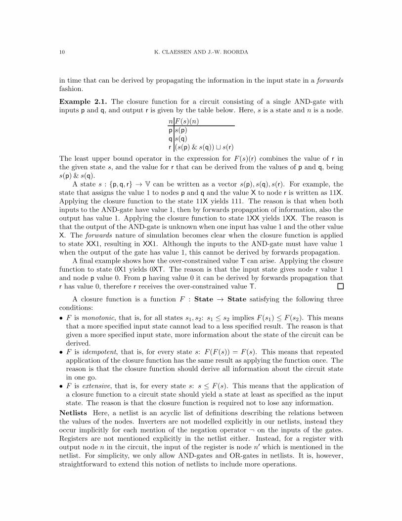
Example 2.1. The closure function for a circuit consisting of a single AND-gate withinputs p and q, and output r is given by the table below. Here, s is a state and n is a node.

n F (s)(n)p s(p)q s(q)r (s(p) & s(q)) ⊔ s(r)

The least upper bound operator in the expression for F (s)(r) combines the value of r inthe given state s, and the value for r that can be derived from the values of p and q, beings(p) & s(q).

A state s : {p, q, r} → V can be written as a vector s(p), s(q), s(r). For example, thestate that assigns the value 1 to nodes p and q and the value X to node r is written as 11X.Applying the closure function to the state 11X yields 111. The reason is that when bothinputs to the AND-gate have value 1, then by forwards propagation of information, also theoutput has value 1. Applying the closure function to state 1XX yields 1XX. The reason isthat the output of the AND-gate is unknown when one input has value 1 and the other valueX. The forwards nature of simulation becomes clear when the closure function is appliedto state XX1, resulting in XX1. Although the inputs to the AND-gate must have value 1when the output of the gate has value 1, this cannot be derived by forwards propagation.

A final example shows how the over-constrained value T can arise. Applying the closurefunction to state 0X1 yields 0XT. The reason is that the input state gives node r value 1and node p value 0. From p having value 0 it can be derived by forwards propagation thatr has value 0, therefore r receives the over-constrained value T.

A closure function is a function F : State → State satisfying the following threeconditions:

• F is monotonic, that is, for all states s1, s2: s1 ≤ s2 implies F (s1) ≤ F (s2). This meansthat a more specified input state cannot lead to a less specified result. The reason is thatgiven a more specified input state, more information about the state of the circuit can bederived.

• F is idempotent, that is, for every state s: F (F (s)) = F (s). This means that repeatedapplication of the closure function has the same result as applying the function once. Thereason is that the closure function should derive all information about the circuit statein one go.

• F is extensive, that is, for every state s: s ≤ F (s). This means that the application ofa closure function to a circuit state should yield a state at least as specified as the inputstate. The reason is that the closure function is required not to lose any information.

Netlists Here, a netlist is an acyclic list of definitions describing the relations betweenthe values of the nodes. Inverters are not modelled explicitly in our netlists, instead theyoccur implicitly for each mention of the negation operator ¬ on the inputs of the gates.Registers are not mentioned explicitly in the netlist either. Instead, for a register withoutput node n in the circuit, the input of the register is node n′ which is mentioned in thenetlist. For simplicity, we only allow AND-gates and OR-gates in netlists. It is, however,straightforward to extend this notion of netlists to include more operations.


Induced Closure Function Given the netlist of a circuit c, the induced closure function

for the circuit, written Fc, can easily be constructed by interpreting each definition in thenetlist as a four-valued gate (see Figure 3). Each

Given a state s, a circuit c, and a circuit node n, we calculate Fc(s)(n) as follows:

• If n is a circuit input or the output of a register, then we define Fc(s)(n) = s(n).• If n is the output of an AND-gate with input nodes p and q, then we define

Fc(s)(n) = (Fc(s)(p) & Fc(s)(q)) ⊔ s(n).

• If n is the output of an OR-gate with input nodes p and q, then we define

Fc(s)(n) = (Fc(s)(p) + Fc(s)(q)) ⊔ s(n).

• If n is the output of an inverter with input node p, then we define

Fc(s)(n) = ¬Fc(s)(p) ⊔ s(n).

This definition is well-defined because netlists are acyclic by definition.

Proposition 2.2. The induced closure function for a circuit is by construction monotonic,

idempotent and extensive.

Proof. The closure function Fc is a composition of the monotonic functions of four-valuednegation, four-valued conjunction and least upper bound, therefore it is monotonic itself.

As netlists are acyclic by definition, we can prove properties by induction over the def-inition of a node. We prove idempotency by proving Fc(Fc(s))(n) = Fc(s)(n) by inductionon the definition of n. Assume n is in the set of input- and state-holding nodes I ∪S, thenFc(Fc(s))(n) = Fc(s)(n) by definition. If n is defined by n = p and q, then:

Fc(Fc(s))(n)= (Fc(Fc(s))(p) & Fc(Fc(s))(q)) ⊔ Fc(s)(n) (definition)= (Fc(s)(p) & Fc(s)(q)) ⊔ Fc(s)(n) (ind. hyp.)= (Fc(s)(p) & Fc(s)(q)) ⊔ (Fc(s)(p) & Fc(s)(q)) ⊔ s(n) (definition)= (Fc(s)(p) & Fc(s)(q)) ⊔ s(n) (property ⊔)= Fc(s)(n) (definition)

A similar argument holds when n is defined by a different gate definition.The extensivity of Fc follows directly from its definition: If n is an input or state holding

node then Fc(s)(n) = s(n), otherwise F (c)(n) is defined as the least upper bound of s(n)and another expression, so s(n) ≤ Fc(s)(n).

2.3. A closure function for sequences. Sequences A sequence of depth d, writtenσ : {0, 1, . . . , d} → State, is a function from a point in time to a circuit state, describingthe behaviour of a circuit over time. The set of all sequences is written Seq. A three-valued

sequence is a sequence that does not assign the value T to any node at any time.The order ≤ and the operators ⊔ and ⊓ are extended to sequences in a point-wise

fashion. That is, the order ≤ on sequences is defined by σ1 ≤ σ2 iff for all n, σ1(n) ≤ σ2(n).Furthermore, (σ1 ⊔ σ2)(n) = (σ1(n) ⊔ σ2(n)), and (σ1 ⊓ σ2)(n) = (σ1(n) ⊓ σ2(n)).Closure for sequences In STE, a circuit is simulated over multiple time steps. Duringsimulation, information is propagated forwards through the circuit and through time, fromeach time step t to time step t+ 1. Note that the initial values of registers are ignored.

To model this forwards propagation of information through time, a closure function for

sequences, notation F→ : Seq → Seq, is used. Given a sequence, the closure function for


sequences calculates all information that can be derived from that sequence by forwardspropagation. The closure function for sequences preserves the depth of the given sequence.

Recall that for every register with output n, the input to the register is node n′. There-fore, the value of node n′ at time t is propagated to node n at time t + 1 in the forwardsclosure for sequences.

Given a circuit state s, the function next calculates the information that is propagatedby the registers, and is defined by:

next(s)(n) =

{

s(n′), n ∈ SX, otherwise

The closure function for sequences F→ is defined in terms of a closure function F . Given aclosure function F for a circuit with a set of outputs of registers S, the closure function for

sequences, written F→ : Seq → Seq, is inductively defined by:

F→(σ)(0) = F (σ(0))F→(σ)(t+ 1) = F ( σ(t+ 1) ⊔ next(F→(σ)(t)) ) (0 ≤ t ≤ d− 1)

Proposition 2.3. The function F→ inherits the properties of being monotonic, idempotent

and extensive from F .

Proof. The closure function F→ is a composition of the monotonic functions, F and leastupper bound, therefore it is monotonic itself.

We prove the idempotency of F→ by proving F→(F→(σ))(t) = F→(σ)(t) by inductionon t.

Suppose t = 0, then

F→(F→(σ))(0)= F (F→(σ)(0)) (definition of F→)= F (F (σ(0)) (definition of F→))= F (σ(0)) (idempotency of F )= F→(σ)(0) (definition of F→))

The induction hypothesis is: F→(F→(σ))(t) = F→(σ)(t) for a fixed t. Suppose that theinduction hypothesis holds, then:

F→(F→(σ))(t + 1)= F (F→(σ)(t+ 1) ⊔ next(F→(F→(σ))(t)) ) (definition of F→)= F (F→(σ)(t+ 1) ⊔ next(F→(σ)(t)) ) (ind. hyp.)

Now we reduce the term F→(σ)(t+ 1) ⊔ next(F→(σ)(t)) further.

F→(σ)(t+ 1) ⊔ next(F→(σ)(t))= F ( σ(t+ 1) ⊔ next(F→(σ)(t))) ⊔ next(F→(σ)(t)) (def. F→)= F ( σ(t+ 1) ⊔ next(F→(σ)(t))) (F extensive, prop. ⊔)

Thus:F→(F→(σ))(t + 1)

= F (F→(σ)(t + 1) ⊔ next(F→(σ)(t)) ) (see above)= F (F ( σ(t+ 1) ⊔ next(F→(σ)(t)))) (see above)= F ( σ(t+ 1) ⊔ next(F→(σ)(t))) F idempotent= F→(σ)(t+ 1) (def. F→)

Finally, F→ being extensive follows directly from the definition of F→ and the propertiesof ⊔.


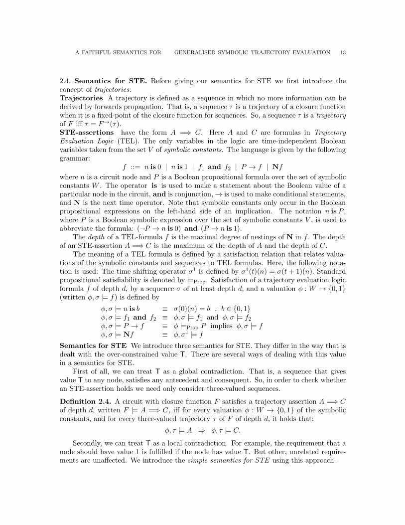
2.4. Semantics for STE. Before giving our semantics for STE we first introduce theconcept of trajectories:Trajectories A trajectory is defined as a sequence in which no more information can bederived by forwards propagation. That is, a sequence τ is a trajectory of a closure functionwhen it is a fixed-point of the closure function for sequences. So, a sequence τ is a trajectory

of F iff τ = F→(τ).STE-assertions have the form A =⇒ C. Here A and C are formulas in Trajectory

Evaluation Logic (TEL). The only variables in the logic are time-independent Booleanvariables taken from the set V of symbolic constants. The language is given by the followinggrammar:

f ::= n is 0 | n is 1 | f1 and f2 | P → f | Nf

where n is a circuit node and P is a Boolean propositional formula over the set of symbolicconstants W . The operator is is used to make a statement about the Boolean value of aparticular node in the circuit, and is conjunction, → is used to make conditional statements,and N is the next time operator. Note that symbolic constants only occur in the Booleanpropositional expressions on the left-hand side of an implication. The notation n is P ,where P is a Boolean symbolic expression over the set of symbolic constants V , is used toabbreviate the formula: (¬P → n is 0) and (P → n is 1).

The depth of a TEL-formula f is the maximal degree of nestings of N in f . The depthof an STE-assertion A =⇒ C is the maximum of the depth of A and the depth of C.

The meaning of a TEL formula is defined by a satisfaction relation that relates valua-tions of the symbolic constants and sequences to TEL formulas. Here, the following nota-tion is used: The time shifting operator σ1 is defined by σ1(t)(n) = σ(t + 1)(n). Standardpropositional satisfiability is denoted by |=Prop. Satisfaction of a trajectory evaluation logicformula f of depth d, by a sequence σ of at least depth d, and a valuation φ : W → {0, 1}(written φ, σ |= f) is defined by

φ, σ |= n is b ≡ σ(0)(n) = b , b ∈ {0, 1}φ, σ |= f1 and f2 ≡ φ, σ |= f1 and φ, σ |= f2φ, σ |= P → f ≡ φ |=Prop P implies φ, σ |= fφ, σ |= Nf ≡ φ, σ1 |= f

Semantics for STE We introduce three semantics for STE. They differ in the way that isdealt with the over-constrained value T. There are several ways of dealing with this valuein a semantics for STE.

First of all, we can treat T as a global contradiction. That is, a sequence that givesvalue T to any node, satisfies any antecedent and consequent. So, in order to check whetheran STE-assertion holds we need only consider three-valued sequences.

Definition 2.4. A circuit with closure function F satisfies a trajectory assertion A =⇒ Cof depth d, written F |= A =⇒ C, iff for every valuation φ : W → {0, 1} of the symbolicconstants, and for every three-valued trajectory τ of F of depth d, it holds that:

φ, τ |= A ⇒ φ, τ |= C.

Secondly, we can treat T as a local contradiction. For example, the requirement that anode should have value 1 is fulfilled if the node has value T. But other, unrelated require-ments are unaffected. We introduce the simple semantics for STE using this approach.


Definition 2.5. A circuit with closure function F simply satisfies a trajectory assertionA =⇒ C of depth d, written F |=Simple A =⇒ C, iff for every valuation φ : W → {0, 1} ofthe symbolic constants, and for every trajectory τ of F of depth d, it holds that:

φ, τ |= A ⇒ φ, τ |= C.

The simple semantics turns out to be useful when we compare the proving power ofSTE and GSTE in a precise way in Sect. 4. In the simple semantics, it is for examplemeaningful to talk about what happens in a sequence before certain nodes get a value T

forced by an antecedent.Finally, we can treat T as an error. That is, if a node is required to have value T by the

antecedent of an STE-assertion, the STE-assertion is not true. This is the default approachtaken in Intel’s in-house verification toolkit Forte [3]: it raises an antecedent failure if anode is required to have value T by the antecedent. We call this semantics, the cautious

semantics for STE.

Definition 2.6. A circuit with closure function F cautiously satisfies a trajectory assertionA =⇒ C of depth d, written F |=Cautious A =⇒ C, if both F |= A =⇒ C and for everyvaluation φ of the symbolic constants there exists a three-valued trajectory τ of depth dsuch that φ, τ |= A.

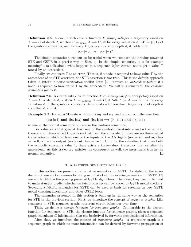
Example 2.7. For an AND-gate with inputs in1 and in2, and output out, the assertion

(out is 1) and (in1 is a) and (in2 is b) =⇒ (in1 is 1) and (in2 is 1)

is true in the normal semantics but not in the cautious semantics.For valuations that give at least one of the symbolic constants a and b the value 0,

there are no three-valued trajectories that meet the antecedent: there are no three-valuedtrajectories in which at least one of the inputs of the AND-gate (nodes in1 and in2) hasvalue 0, while the output (node out) has value 1. Only for the valuation that gives boththe symbolic constants value 1, there exists a three-valued trajectory that satisfies theantecedent. As this trajectory satisfies the consequent as well, the assertion is true in thenormal semantics.

3. A Faithful Semantics for GSTE

In this section, we present an alternative semantics for GSTE. As stated in the intro-duction, there are two reasons for doing so. First of all, the existing semantics for GSTE [17]are not faithful to the proving power of GSTE algorithms. Therefore, they cannot be usedto understand or predict whether certain properties can be proven by GSTE model checkers.Secondly, a faithful semantics for GSTE can be used as basis for research on new GSTEmodel checking algorithms and other GSTE tools.

The semantics presented in this section is built up in the same way as the semanticsfor STE in the previous section. First, we introduce the concept of sequence graphs. Likesequences in STE, sequence graphs represent circuit behaviour over time.

Then, we define a closure function for sequence graphs. Comparable to the closurefunction for sequences in STE, the closure function for sequence graphs, given a sequencegraph, calculates all information that can be derived by forwards propagation of information.

After that, we introduce the concept of trajectory graphs. A trajectory graph is asequence graph in which no more information can be derived by forwards propagation of


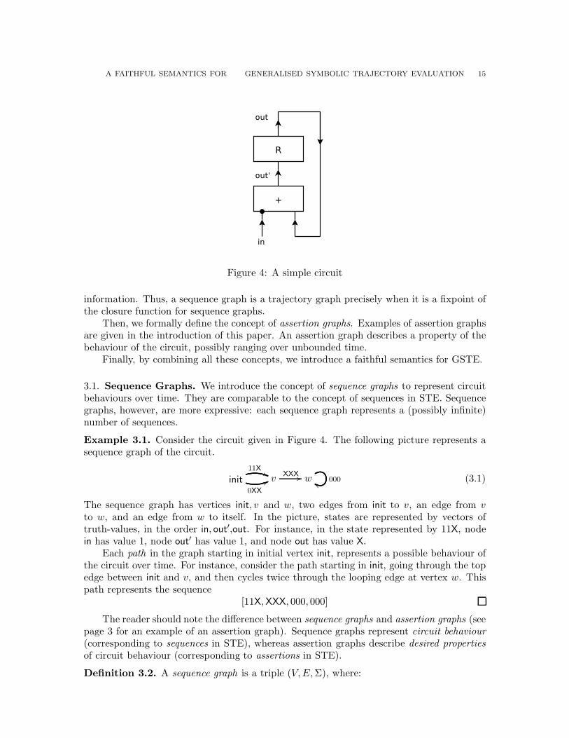
Figure 4: A simple circuit

information. Thus, a sequence graph is a trajectory graph precisely when it is a fixpoint ofthe closure function for sequence graphs.

Then, we formally define the concept of assertion graphs. Examples of assertion graphsare given in the introduction of this paper. An assertion graph describes a property of thebehaviour of the circuit, possibly ranging over unbounded time.

Finally, by combining all these concepts, we introduce a faithful semantics for GSTE.

3.1. Sequence Graphs. We introduce the concept of sequence graphs to represent circuitbehaviours over time. They are comparable to the concept of sequences in STE. Sequencegraphs, however, are more expressive: each sequence graph represents a (possibly infinite)number of sequences.

Example 3.1. Consider the circuit given in Figure 4. The following picture represents asequence graph of the circuit.

init

11X((

0XX

66 vXXX // w 000ff (3.1)

The sequence graph has vertices init, v and w, two edges from init to v, an edge from vto w, and an edge from w to itself. In the picture, states are represented by vectors oftruth-values, in the order in, out′,out. For instance, in the state represented by 11X, nodein has value 1, node out′ has value 1, and node out has value X.

Each path in the graph starting in initial vertex init, represents a possible behaviour ofthe circuit over time. For instance, consider the path starting in init, going through the topedge between init and v, and then cycles twice through the looping edge at vertex w. Thispath represents the sequence

[11X,XXX, 000, 000]

The reader should note the difference between sequence graphs and assertion graphs (seepage 3 for an example of an assertion graph). Sequence graphs represent circuit behaviour(corresponding to sequences in STE), whereas assertion graphs describe desired properties

of circuit behaviour (corresponding to assertions in STE).

Definition 3.2. A sequence graph is a triple (V,E,Σ), where:


• V is a finite set of vertices containing the initial vertex init.• E is a finite set of directed edges between vertices. Each edge e has a start vertex start(e)and an end vertex end(e). Multiple edges between two vertices are allowed.

• Σ : E → State is a function from edges to circuit states.

We say that sequence graphs (V1, E1,Σ1) and (V2, E2,Σ2) are of the same shape iff V1 = V2

and E1 = E2. The set of all sequence graphs is denoted SeqGraph.

Usually, a sequence graph is identified by the function Σ only.The order ≤ and the operators ⊔ and ⊓ on the domain {0, 1,X,T} are extended in a

point-wise fashion to pairs of sequence graphs of the same shape. That is, the order ≤ onsequence graphs is defined by Σ1 ≤ Σ2 iff for all edges e and nodes n, Σ1(e)(n) ≤ Σ2(e)(n).Furthermore, (Σ1 ⊔ Σ2)(e)(n) = (σ1(e)(n) ⊔ σ2(e)(n)) and (Σ1 ⊓ Σ2)(n) = (Σ1(e)(n) ⊓Σ2(e)(n)).

An edge is initial if it starts in the initial vertex init. We define the set of incomingedges of an edge e, written in(e) by:

in(e) = { e′ ∈ E | start(e) = end(e′)}

A path of depth d is a list of edges ρ = (e0, e1, . . . , ed) such that for each i, start(ei+1) =end(ei). An initial path is a path whose first edge is initial.

A finite initial path ρ of depth d in a sequence graph Σ represents the sequence seq(Σ, ρ)of depth d defined by

seq(Σ, ρ)(t) = Σ(ρ(t)).

A sequence graph Σ represents the set of sequences seq(Σ) defined by

seq(Σ) = {seq(Σ, ρ) | ρ is a finite initial path in Σ}

We will only consider sequence graphs in which each edge and each vertex is reachable fromthe initial vertex init. That is, we require that for each edge there exists an initial pathcontaining the edge, and for each vertex there exists an initial path containing the vertex.The reason is that states at unreachable edges cannot appear in the sequences representedby the sequence graph.

Example 3.3. The sequence graph (3.1) represents the following infinite set of sequences:

[11X][11X,XXX][11X,XXX, 000][11X,XXX, 000, 000]. . .[0XX][0XX,XXX][0XX,XXX, 000][0XX,XXX, 000, 000]. . .

The sequence graph

init111 // v

XXX

�� 000 // w


represents the following infinite set of sequences:

[111][111, 000][111,XXX][111,XXX, 000][111,XXX,XXX][111,XXX,XXX, 000]. . .

3.2. Trajectory Graphs and Closure Functions. We introduce the concept of trajec-tory graphs to represent sequence graphs in which no more information can be derived byforwards propagation of information. Trajectory graphs are comparable to the concept oftrajectories in STE.

In order to define trajectory graphs, we define a closure function for sequence graphs,written F ◦ : SeqGraph → SeqGraph. The idea is that such a closure function, givena sequence graph, derives all information that can be derived by forwards propagation.Then, a trajectory graph is defined as a fixpoint of this closure function.

Before doing so, let us first get some more intuition on desired properties for a closurefunction for sequence graphs. Recall that a sequence graph represents a (possibly infinite)collection of sequences. Each initial path ρ in the graph represents a sequence seq(Σ, ρ) asdefined before.

Furthermore, recall, from the introduction, when a circuit satisfies a GSTE assertiongraph, the circuit should also satisfy all STE-assertion corresponding to finite initial pathsin the assertion graphs.

Therefore, given a sequence graph and an initial path ρ in the graph, we expect that theclosure function on sequence graphs F ◦ for the edges in ρ derives at most the informationas the closure function for sequences F→ does for the sequence seq(Σ, ρ). The reasonfor requiring this is that if the closure function on sequence graphs were to derive moreinformation for a particular sequence in the sequence graph than the closure function onsequences, then we could construct a GSTE assertion graph that is satisfied by the circuit,but that contains a path corresponding to an untrue STE-assertion.

So, we require the following property:

Property 3.4. A closure function F ◦ for sequence graphs derives no more information

than a closure function on sequences F→, if for all sequence graphs Σ and initial paths ρ,

seq(F ◦(Σ), ρ) ≤ F→(seq(Σ, ρ))

The closure function for sequence graphs is allowed to derive less information for aparticular path than the closure function for sequences does. The reason is that an edgemight be reached via different initial paths. If, for these paths, the closure function forsequences derives conflicting values for a circuit node at that edge, the above propertyforces the circuit node to take on value X. We elaborate on this in Example 3.6 on page 19.

Defining a closure function for sequence graphs is a greater challenge than defining aclosure function for sequences. There are two reasons for this.

First of all, in STE, for a state at time t + 1, there is precisely one “previous” state,namely the state at time t. So, it is clear how the information from previous points in time


should be propagated. In GSTE, however, a state at an edge can have multiple predecessors.So, we have to decide how to combine information from incoming edges.

Secondly, in STE-sequences, the state at each time-point depends only on the previousstates, and, thus, never on itself. In GSTE sequence graphs, however, cycles may be present,therefore a state may, via a cycle, depend on itself.

In the following, we gradually construct a closure function for sequence graphs byconsidering closure functions for increasingly more complex sets of sequence graphs. First,we only consider linear sequence graphs, then we look at acyclic sequence graphs, andfinally we consider general sequence graphs.

Linear sequence graphs. Let us take one step at the time. So, first, assume we have asequence graph where each vertex has at most one successor and at most one predecessor,and no cycles are present. Such a sequence graph has the following form:

init // v1 // v2 // . . . // vd

For edges that have exactly one incoming edge, we define the function pre {pre(e)} = in(e).(Recall that in(e) is the set of all incoming edges of e.)

For the above sequence graph, a closure function F ◦line can be defined in the same way

as in STE. For the initial edge, no information is propagated from a previous time-point,so only closure of the initial state is needed. For each other time-point, information fromthe previous state should be propagated.

This yields the closure function F ◦line:

F ◦line(Σ)(e) =

{

F (Σ(e)), e is initialF (Σ(e) ⊔ next( F ◦

line(Σ)(pre(e)) ), otherwise

The function F ◦line is well defined as the graphs we consider here are acyclic and edges have

at most one predecessor. Note the similarity with the closure function for sequences F→ onpage 12.

Note that, just like in STE, the initial values of registers are ignored.F ◦line calculates precisely the same information as F→. That is, for each initial path ρ

in a sequence graph Σ of the above form,

seq(F ◦line(Σ), ρ) = F→(seq(Σ, ρ)).

Acyclic sequence graphs. Now, let us consider a more general situation: an acyclic graph.

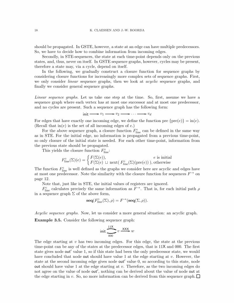
Example 3.5. Consider the following sequence graph:

init

11X((

000

66 vXXX // w

The edge starting at v has two incoming edges. For this edge, the state at the previoustime-point can be any of the states at the predecessor edges, that is 11X and 000. The firststate gives node out′ value 1, so if this state had been the only predecessor state, we wouldhave concluded that node out should have value 1 at the edge starting at v. However, thestate at the second incoming edge gives node out′ value 0, so according to this state, nodeout should have value 1 at the edge starting at v. Therefore, as the two incoming edges donot agree on the value of node out′, nothing can be derived about the value of node out atthe edge starting in v. So, no more information can be derived from this sequence graph.


So, only if all the states of the incoming edges agree on a Boolean value of an input toa register, should this value be propagated to the output of the register. Thus, to combinethe values on the inputs of the register, the greatest lower bound should be used. This yieldsthe closure function F ◦

nocycle:

F ◦nocycle(Σ)(e) =

{

F (Σ(e)), e is initialF (Σ(e) ⊔ ⊓

i∈in(e)next( F ◦

nocycle(Σ)(i)) ), otherwise

Example 3.6. Applied to the sequence graph in Example 3.5, the closure function yieldsthe same sequence graph. In the graph, the top edge between init and v gives value 1 toout′, the bottom edge gives value 0 to this node, so 0 ⊓ 1 = X is propagated for the valueof node out for the edge starting in v.

In this example, the closure function for sequence graphs derives less information thanthe closure function for sequences for the paths in the assertions. The reason is that thegreatest lower-bound operator is used to combine conflicting information from incomingedges.

Applied to

init

1XX((

1XX

66 vXXX // w

the closure function yields

init

11X((

11X

66 vX11 // w

As both incoming edges give value 1 to node out′ this value is propagated to node out.

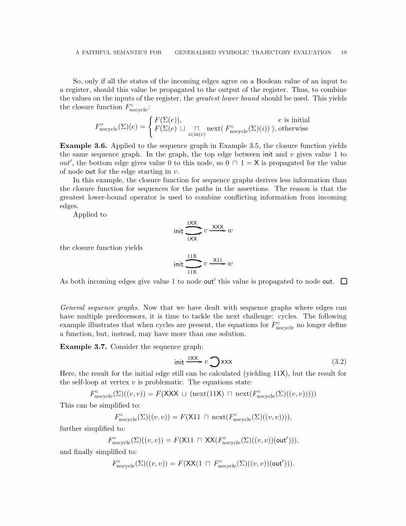
General sequence graphs. Now that we have dealt with sequence graphs where edges canhave multiple predecessors, it is time to tackle the next challenge: cycles. The followingexample illustrates that when cycles are present, the equations for F ◦

nocycle no longer definea function, but, instead, may have more than one solution.

Example 3.7. Consider the sequence graph:

init1XX // v XXXee (3.2)

Here, the result for the initial edge still can be calculated (yielding 11X), but the result forthe self-loop at vertex v is problematic. The equations state:

F ◦nocycle(Σ)((v, v)) = F (XXX ⊔ (next(11X) ⊓ next(F ◦

nocycle(Σ)((v, v)))))

This can be simplified to:

F ◦nocycle(Σ)((v, v)) = F (X11 ⊓ next(F ◦

nocycle(Σ)((v, v)))),

further simplified to:

F ◦nocycle(Σ)((v, v)) = F (X11 ⊓ XX(F ◦

nocycle(Σ)((v, v))(out′))),

and finally simplified to:

F ◦nocycle(Σ)((v, v)) = F (XX(1 ⊓ F ◦

nocycle(Σ)((v, v))(out′))).


This equation can be rewritten to:

F ◦nocycle(Σ)((v, v)) = (λs.F (XX(1 ⊓ s((v, v))(out′))) F ◦

nocycle(Σ)((v, v))

This equation has as solutions precisely the fixpoints of

(λs.F (XX(1 ⊓ s(out′)))

The two fixed-points are XXX or X11.The first fixed-point yields the following sequence graph:

init11X // v XXXee (3.3)

This contradicts our intuition: if at the first point in time node in has value 1, then weexpect that, from the next time-point on, node out and out′ have value 1 as well. So, onlythe second fixed-point gives the expected sequence graph:

init11X // v X11ee (3.4)

So, in general, when cycles are introduced, the equations for F ◦nocycle no longer define a

function: the equations may have more than one solution. Let us study this set of solutionsmore closely.

To do so, we define, for a given sequence graph Σ, the function F ◦Σ : SeqGraph →

SeqGraph by:

F ◦Σ(∆)(e) =

{

F (Σ(e)), e is initialF ( Σ(e) ⊔ ⊓

i∈in(e)next(∆(i)) ), otherwise

Using this, the equations for F ◦nocycle can be rewritten to:

F ◦nocycle(Σ) = F ◦

Σ(F◦nocycle(Σ))

The solutions of this equation are the set of fixpoints of F ◦Σ. For example, for Σ equal to

sequence graph (3.2) the fixpoints are sequence graphs (3.3) and (3.4).The following lemma states that each fixpoint satisfies Property 3.4.

Lemma 3.8. For each ∆ that is a fixpoint of F ◦Σ and for each initial path ρ in the sequence

graph Σ, it holds that:

seq(∆, ρ) ≤ F→(seq(Σ, ρ))

Proof. The proof is by induction on the position in the sequence. The base-case (t = 0)follows directly from the definitions of seq and F→. The induction hypothesis is:

seq(∆, ρ)(t) ≤ (F→(seq(Σ, ρ)))(t)

If ρ(t+ 1) is not initial, then

seq(∆, ρ)(t + 1) = F ( Σ(ρ(t+ 1)) ⊔ ⊓i∈in(ρ(t+1))

next(∆(i)) )

Now:

⊓i∈in(ρ(t+1))

next(∆(i))

≤ next(∆(ρ(t))) (ρ(t) ∈ in(ρ(t+ 1))= next(seq(∆, ρ)(t))) (Definition seq)≤ next(F→(seq(Σ, ρ))(t)) ((Induction hypothesis and monotonicity next)


Thus,seq(∆, ρ)(t+ 1) ≤ F ( seq(Σ, ρ)(t+ 1) ⊔ next(F→(seq(Σ, ρ))(t)) )

So, by the definition of F→,

seq(∆, ρ)(t+ 1) ≤ F→(seq(Σ, ρ))(t+ 1)

The case for ρ(t+ 1) is initial is similar but easier.

The question now is: which fixpoint should the closure function for sequence graphschoose? As each fixpoint satisfies Property 3.4, it is sound to choose any of them. Thefollowing property states there exists a unique greatest fixpoint.

Proposition 3.9. For each Σ, the function F ◦Σ has a unique greatest fixpoint.

Proof. It is easy to see that F ◦Σ is monotonic. The collection of sequence graphs with the

same vertices and edges as Σ and giving values to the same circuit nodes as Σ is finite andforms, together with the order ≤ on sequence graphs, a complete lattice. So, by Tarski’sfixpoint theorem [13], F ◦

Σ has a greatest fixpoint.

As each fixpoint satisfies Property 3.4, we can safely choose the greatest one, giving themost information. Thus, we define the closure function for sequence graphs as follows:

Definition 3.10. Given a closure function F , the closure function for sequence graphs,written F ◦ : SeqGraph → SeqGraph is defined by:

F ◦(Σ) = gfp∆.F ◦Σ(∆)

Proposition 3.11. Given a closure function F , F ◦ is a closure function as well.

Proof. Suppose F is a closure function, we have to prove that F ◦ is monotonic, extensiveand idempotent. F ◦ being extensive follows directly from the definition of F ◦.

We now prove that F ◦ is monotonic. Suppose Σ1 ≤ Σ2, ∆1 = F ◦(Σ1) and ∆2 = F ◦(Σ2),then

∆1 = F ◦Σ1(∆1) ≤ F ◦

Σ2(∆1)

Tarski’s fixpoint theorem [13] states that

gfp∆.F ◦Σ2(∆) = ⊔{∆ |∆ ≤ F ◦

Σ2(∆)}

Thus ∆1 ≤ gfp∆.F ◦Σ2

(∆) = ∆2.

Finally, we prove that F ◦ is idempotent. Suppose F ◦(Σ) = ∆ and F ◦(∆) = ∆′. Weneed to prove that ∆ = ∆′. By monotonicity of F ◦ follows ∆ ≤ ∆′. We prove that ∆′ ≤ ∆by proving that ∆′ is a fixpoint of F ◦

Σ (then, because ∆ is the greatest fix-point of F ◦Σ, it

follows that ∆′ ≤ ∆). The case for when e is initial is trivial. Suppose e is not initial.

F ◦Σ(∆

′)(e)= F (Σ(e) ⊔ ⊓

i∈in(e)next(∆′(i))) (Definition F ◦

Σ)

= F (Σ(e) ⊔ ⊓i∈in(e)

next(∆(i)) ⊔ ⊓i∈in(e)

next(∆′(i))) (Prop ⊔, ∆ ≤ ∆′)

= F (F (Σ(e) ⊔ ⊓i∈in(e)

next(∆(i))) ⊔ ⊓i∈in(e)

next(∆′(i))) (F is closure function)

= F (∆(e) ⊔ ⊓i∈in(e)

next(∆′(i))) (∆ is fixpoint of F ◦Σ)

= ∆′(e) (∆′ is fixpoint of F ◦∆)


3.2.1. Trajectory Graphs. We define a trajectory graph of F as a sequence graph that is afixpoint of F ◦.

Definition 3.12. A sequence graph Σ is a trajectory graph of a closure function F , if

F ◦(Σ) = Σ

3.3. Assertion Graphs. In GSTE, circuit properties are given by assertion graphs. Anexample of an assertion graph is:

initin is 1/·

// v ·/out is 1ee (3.5)

In the assertion graph, each edge is labelled with a pair A/C, here A is called the antecedentand C is called the consequent. Just like in STE, the antecedent represents assumptionsmade, and the consequent represents requirements.

Both A and C are, like in STE, formulas in trajectory evaluation logic (TEL). However,as each edge represents the state of a single time-point, no occurrences of the next-timeoperator N are allowed. We call the subset of TEL in which no next-time operators occurGTEL.

The assertion graph above states that if at some time point, node in has value 1, thenat each later time-point node out has value 1 as well.

Definition 3.13. An assertion graph is a four-tuple G = (V,E, ant , cons). Here, V is aset of vertices containing a vertex init which is called the initial vertex, E is a set of edgesbetween the vertices. Finally, ant , cons : E → GTEL are functions from edges to formulasin GTEL.

Recall that path is called initial iff it starts in the initial vertex init. A finite initial pathρ of depth d in an assertion graph G represents an STE assertion Ass(G, ρ) defined by

Ass(G, ρ) = ( and0≤i≤d

Niant(ρ(t))) ⇒ ( and0≤i≤d

Nicons(ρ(t)))

An assertion graph represents a (possibly infinite) collection of STE-assertions: for eachfinite initial path ρ in the graph, an STE-assertion Ass(G, ρ). The set of STE-assertions inassertions graph G, written Ass(G), is defined by:

Ass(G) = {Ass(G, ρ) | ρ is a finite initial path in G}

Example 3.14. Assertion graph (3.5) above represents the following infinite set of STE-assertions:

in is 1 =⇒ N(out is 1)in is 1 =⇒ N(out is 1) and NN(out is 1)in is 1 =⇒ N(out is 1) and NN(out is 1) and NNN(out is 1)

. . .

The idea is that when a circuit satisfies a GSTE assertion graph, the circuit graph alsosatisfies all STE assertions in the assertion graph. The converse, however, does not hold,as we will see in the next section.


3.4. Satisfiability. Satisfaction of a GTEL-formula f , by a circuit state s : State and avaluation φ : W → {0, 1} of the symbolic constants (written φ, s |= f) is defined by

φ, s |= n is b ≡ σ(0)(n) = b , b ∈ {0, 1}φ, s |= f1 and f2 ≡ φ, s |= f1 and φ, s |= f2φ, s |= P → f ≡ φ |=Prop P implies φ, s |= f

Example 3.15. If s(in) = 1 and s(out) = 0, and φ(a) = 1 and φ(b) = 0, then

φ, s |= (in is a) and (out is b) and (in is ¬(a ∧ b))

We say that a sequence graph (V,E,Σ) satisfies a function f : E → GTEL, f ∈{ant , cons} and a valuation φ : W → {0, 1} of the symbolic constants, written φ,Σ |= f , iffor all edges e:

φ,Σ(e) |= f(e)

Note that the definition of satisfaction above requires that the shape of the sequence graphbe identical to the shape of the assertion graph from which the antecedent or consequent istaken.

Example 3.16. If G = (V,E, ant , cons) is assertion graph (3.5), Σ1 is sequence graph (3.2),and Σ2 is sequence graph (3.4), then for any φ: φ,Σ1 |= ant , φ,Σ2 |= ant , φ,Σ1 6|= cons ,and φ,Σ2 |= cons .

Just like in STE, in GSTE, there are several ways of dealing with the over-constrainedvalue T. We can treat T just as any other value, leading to the simple semantics of GSTE.Or, we can treat an over-constrained value as an error, leading to the cautious semantics

of GSTE.In GSTE, however, we cannot treat T as a contradiction in the same way as we did

in STE. The reason is the following. Consider a semantics in which a sequence graph thatassigns a T to a circuit node at an edge satisfies any antecedent and consequent. In sucha semantics, GSTE assertion graphs containing false STE-assertions may still be true. Forexample, given a GSTE assertion graph containing a false STE assertion, we can simplyadd a fresh initial edge with an inconsistent antecedent, making the GSTE assertion true.

If, instead, we require a T value at each path in the graph to deem a sequence graphcontradictory, this problem does not occur. However, as the implementation of such asemantics in a GSTE model checker seems cumbersome, we will not elaborate on such asemantics further.

In the definition of simple satisfaction for GSTE, the value T is treated just like anyother value, and models a local conflict of demands made by the assertion. In this paper,we consider this the ‘standard’ semantics for GSTE. As explained in Sect. 4, this turns outto correspond well with what most GSTE algorithms do in practice.

Definition 3.17. We say that a closure function F simply satisfies an assertion graphG = (V,E, ant , cons), written F |=Simple G, if for all assignments of symbolic constantsφ : W → {0, 1}, trajectory graphs Σ,

Σ |= ant ⇒ Σ |= cons .

Example 3.18. If G = (V,E, ant , cons) is assertion graph (3.5), and F is the closurefunction for the circuit in Figure 4, then F |=Simple G.

This can be explained as follows. It is easy to see that, for any φ, sequence graph(3.2) is the weakest sequence graph that makes the antecedent of G true. Let us call this


sequence graph Σ. Trajectory graph (3.4) is F ◦(Σ). We claim that F ◦(Σ) is the weakesttrajectory graph satisfying ant . This can be proven easily. Suppose T is a trajectory graphsatisfying ant , then Σ ≤ T , so by monotonicity of F ◦ and because T is a fix-point of F ◦,F ◦(Σ) ≤ F ◦(T ) = T . Thus, as the weakest trajectory graph satisfying ant also satisfiescons , all trajectory graphs that satisfy ant satisfy cons as well. So, F |=Simple G.

In Section 5, we explain that, in the general case, to check whether a circuit simplysatisfies an assertion graph, we only have to, for each φ, consider the weakest trajectorygraph that satisfies the antecedent ant .

In the definition of cautious satisfaction for GSTE, the value T is treated as an error.

Definition 3.19. We say that a circuit model F , cautiously satisfies an assertion graphG = (V,E, ant , cons), written F |=Cautious G, if F simply satisfies G and for all assignmentsof symbolic constants φ : W → {0, 1}, there exists a trajectory graph Σ of F such thatΣ |= ant .

The following example illustrates the difference between the two definitions.

Example 3.20. The circuit in Figure 4 simply satisfies the following assertion graph. Itdoes, however, not cautiously satisfy it.

initin is 1/·

// v out is 0/out is 1ee

4. Comparing with STE

In this section we compare STE with GSTE. The purpose is to make the relationshipbetween STE and GSTE model checking clear.

The following proposition states that if a closure function satisfies an assertion graph,it simply satisfies all STE-assertions in the assertion graph as well.

Proposition 4.1. Given an assertion graph G = (V,E, ant , cons) for a circuit with closure

function F :

F |= G ⇒ (for all assertions (A =⇒ C) ∈ Ass(G) : F |=Simple (A =⇒ C))

Proof. Suppose F |= G, ρ is a finite path of depth d in G, A =⇒ C = Ass(G, ρ), φ avaluation of the symbolic constants, and τ a trajectory of F of depth d such that φ, τ |= A.We need to prove that φ, τ |= C.

Let Σ be the sequence graph that has the same shape as assertion graph G and isfurther defined by:

Σ(e) = ⊓0≤t≤d,ρ(t)=e

τ(t)

Note that Σ(e)(n) = T for edges not in the path ρ. We now prove that φ,Σ |= ant . Asτ |= A, and A = and

0≤t≤dNtant(ρ(t))), for each t holds:

φ, τ(t) |= ant(ρ(t))

Thus for all e ∈ E:φ, ⊓

t∈N,ρ(t)=eτ(t) |= ant(e)


Thus, φ,Σ |= ant . As F ◦ is extensive, φ, F ◦(Σ) |= ant as well. As F ◦(Σ) is a trajectorygraph, and F |= G, it holds that φ, F ◦(Σ) |= cons . By Property 3.4:

seq(F ◦(Σ), ρ) ≤ F→(seq(Σ, ρ))

Thus:seq(F ◦(Σ), ρ) ≤ F→(τ) = τ

Now, as F ◦(Σ) |= cons , for all e ∈ E:

φ,Σ(e) |= cons(e)

Thus:φ, ⊓

0≤t≤d,ρ(t)=eτ(t) |= cons(ρ(t))

As C = and0≤i≤d

Nicons(ρ(t))), it follows that φ, τ |= C.

The converse

(for all assertions (A =⇒ C) ∈ Ass(G) : F |=Simple (A ⇒ C)) ⇒ F |= G

however, is not true. The reason is that GSTE combines conflicting information betweenincoming edges by using the greatest lower bound operator. This is illustrated by thefollowing example.

Example 4.2. Consider the following circuit:

The induced closure function of this circuit satisfies the STE-assertions p′ is 1 =⇒ N(out is 1)and p′ is 0 =⇒ N(out is 1). Consider the following sequence graph. In the picture, statesare represented by vectors of truth-values, in the order p′, p, out.

init

1XX((

0XX

66 vXXX // w

The sequence graph is a trajectory graph of the closure function. Thus, the closure functiondoes not satisfy the below GSTE assertion graph.

init

p′ is 1/·++

p′ is 0/·

33 v·/out is 1

// w

The following example shows that if a GSTE assertion graph is cautiously satisfied(that is, no node has to assume value T to satisfy the antecedent), there may still be anSTE-assertion represented by the assertion graph that is not cautiously satisfied.


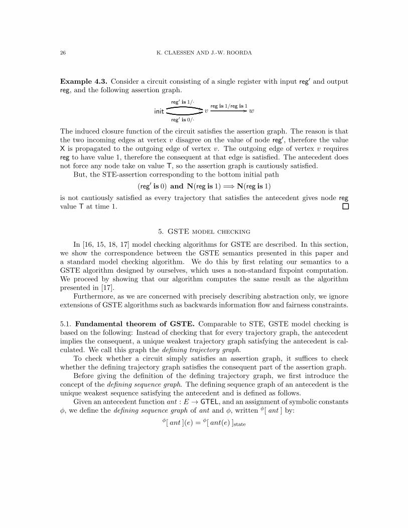
Example 4.3. Consider a circuit consisting of a single register with input reg′ and outputreg, and the following assertion graph.

init

reg′ is 1/·++

reg′ is 0/·

33 vreg is 1/reg is 1

// w

The induced closure function of the circuit satisfies the assertion graph. The reason is thatthe two incoming edges at vertex v disagree on the value of node reg′, therefore the valueX is propagated to the outgoing edge of vertex v. The outgoing edge of vertex v requiresreg to have value 1, therefore the consequent at that edge is satisfied. The antecedent doesnot force any node take on value T, so the assertion graph is cautiously satisfied.

But, the STE-assertion corresponding to the bottom initial path

(reg′ is 0) and N(reg is 1) =⇒ N(reg is 1)

is not cautiously satisfied as every trajectory that satisfies the antecedent gives node reg

value T at time 1.

5. GSTE model checking

In [16, 15, 18, 17] model checking algorithms for GSTE are described. In this section,we show the correspondence between the GSTE semantics presented in this paper anda standard model checking algorithm. We do this by first relating our semantics to aGSTE algorithm designed by ourselves, which uses a non-standard fixpoint computation.We proceed by showing that our algorithm computes the same result as the algorithmpresented in [17].

Furthermore, as we are concerned with precisely describing abstraction only, we ignoreextensions of GSTE algorithms such as backwards information flow and fairness constraints.

5.1. Fundamental theorem of GSTE. Comparable to STE, GSTE model checking isbased on the following: Instead of checking that for every trajectory graph, the antecedentimplies the consequent, a unique weakest trajectory graph satisfying the antecedent is cal-culated. We call this graph the defining trajectory graph.

To check whether a circuit simply satisfies an assertion graph, it suffices to checkwhether the defining trajectory graph satisfies the consequent part of the assertion graph.

Before giving the definition of the defining trajectory graph, we first introduce theconcept of the defining sequence graph. The defining sequence graph of an antecedent is theunique weakest sequence satisfying the antecedent and is defined as follows.

Given an antecedent function ant : E → GTEL, and an assignment of symbolic constantsφ, we define the defining sequence graph of ant and φ, written φ[ ant ] by:

φ[ ant ](e) = φ[ ant(e) ]state


whereφ[m is b ]state(n) =

{

b, if m=nX, otherwise

φ[ f1 and f2 ]state = φ[ f1 ]state ⊔φ[ f2 ]state

φ[ P → f ]state =

{

φ[ f ]state, if φ |= PX, otherwise

Proposition 5.1. φ[ ant ] is the weakest sequence graph satisfying ant and φ.

Proof. Trivial, by considering one edge at the time and induction on the structure of theantecedent at that edge.

Given an antecedent function ant : E → GTEL, a closure function F , and an assignmentof symbolic constants φ, we define the defining trajectory graph of ant , F and φ, writtenφF [[ ant ]] by:

φF [[ ant ]] = F ◦(φ[ ant ])

Proposition 5.2.φF [[ ant ]] is the weakest trajectory graph satisfying ant.

Proof. From F ◦ being extensive, it follows directly that φ[ant ] ≤ F ◦(φ[ant ]), so φF [[ ant ]] |=

ant .Suppose T is a trajectory graph satisfying ant , then φ[ant ] ≤ T . From monotonicity of

F ◦, it follows that F ◦(ant) ≤ F ◦(T ). As T is a fixpoint of F ◦ it follows that F ◦(ant) ≤ T .

Theorem 5.3 (Fundamental Theorem of GSTE). For each closure function F , assignment

of symbolic constants φ, and assertion graph G = (V,E, ant , cons),

(φ[ cons ] ≤ φF [[ ant ]]) ⇔ F |=Simple G

Proof. Directly from Proposition 5.2.

The fundamental theorem of GSTE states that to check whether a circuit with closurefunction F satisfies an assertion graph, we only have to check that, for each φ, the definingtrajectory graph of F satisfies the consequent.

5.2. GSTE Algorithm. The GSTE algorithm calculates a symbolic representation of thedefining trajectory graph of an antecedent. Then, it checks whether this symbolic definingtrajectory graph meets the consequent.

We first present a scalar version of the algorithm.

5.2.1. A scalar GSTE-algorithm. In (our version of the) scalar GSTE-algorithm, the defin-ing trajectory graph of the antecedent is calculated using the constructive version of Tarski’sfixpoint theorem [13].

Proposition 5.4. For each Σ, the greatest fixpoint of the function F ◦Σ is equal to limit ∆Σ

∗

of the sequence ∆Σk = (F ◦

Σ)k(T). Here, T represents the sequence graph with the same edges

and vertices as Σ that gives value T to each circuit node at each edge.


Proof. A function is continuous if for all sequence d0, d1, d2, . . . such that di+1 ≤ di holds:

f( ⊔k∈N

dk) = ⊔k∈N

f(dk)

The constructive version of Tarski’s fixpoint theorem [13] states that the greatest fixpointof a monotone and continuous function f on a complete lattice is given by: ⊓

k∈Nfk(T).

We will use this version of Tarski’s fixpoint theorem to prove the proposition. First,we prove that each monotonic function on a finite domain is also continuous. Suppose f iscontinuous on a finite domain, and d0, d1, d2, . . . is a sequence such that di+1 ≤ di, then thesequence has a fixpoint d∗, thus:

f( ⊔k∈N

dk) = f(d∗)

By monotonicity of f , also the sequence f(d0), f(d1), f(d2), . . . is increasing, so the sequencehas the fix-point f(d∗) as well. So:

⊔k∈N

f(dk) = f(d∗)

Therefore, F ◦Σ is both monotone and continuous. Thus:

gfp∆.F ◦Σ(∆) = ⊓

k∈N(F ◦

Σ)k(T) = ⊓

k∈N∆Σ

k

We prove by induction on k that ∆Σk+1 ≤ ∆Σ

k for each k.

The case for k = 0 is trivial. The induction hypothesis is ∆Σk+1 ≤ ∆Σ

k . We prove that

∆Σk+2 ≤ ∆Σ

k+1. The case for e is initial is trivial. Suppose e is not initial. Then,

∆Σk+2(e)

= F ◦Σ(∆

Σk+1)(e) (Definition ∆Σ

k+2)= F ( Σ(e) ⊔ ⊓

i∈in(e)next(∆Σ

k+1(i)) ) (Definition F ◦Σ)

≤ F ( Σ(e) ⊔ ⊓i∈in(e)

next(∆Σk (i)) ) (Induction Hypothesis)

= F ◦Σ(∆

Σk+1)(e) (Defintion F ◦

Σ)= ∆Σ

k+1(e) (Definition ∆Σk+1)

So, the sequence ∆Σ0 ,∆

Σ1 ,∆

Σ2 will eventually reach a fixpoint ∆Σ

∗ .Thus:

gfp∆.F ◦Σ(∆) = ∆Σ

∗

Definition 5.5 (Scalar GSTE-algorithm). Given an assertion graph G, and a closure func-tion F , the scalar GSTE-algorithm calculates for every φ the defining trajectory graphφF [[ ant ]] by calculating ∆

φ[ ant ]∗ and checks whether

φ[ cons ] ≤ φF [[ ant ]]

If this check fails for any φ the algorithm returns False, otherwise it returns True.

Proposition 5.6. The scalar algorithm is sound and complete with respect to the presented

semantics for GSTE.

Proof. Directly from the fundamental theorem of GSTE and Proposition 5.4.


Comparing with earlier presentation In [17] the fixpoint is calculated in a slightlydifferent way. If we adjust the presentation to use the closure function F instead of atransition relation, the following sequence is defined for a given sequence graph Σ:

ΓΣ0 (e) =

{

F (Σ(e)), e is an initial edgeT, otherwise

ΓΣk+1(e) = ΓΣ

k (e) ⊓ F ( Σ(e) ⊔ ⊓i∈in(e)

next(∆k(i)) )

Proposition 5.7. For each Σ, ΓΣ∗ = ∆Σ

∗ .

Proof. By definition,

∆Σ0 (e)(n) = T

∆Σk+1(e) =

{

F (Σ(e)), e is initialF ( Σ(e) ⊔ ⊓

i∈in(e)next(∆k(i)) ), otherwise

We prove by induction on k that for each initial edge e, for each k, ΓΣk = F (Σ(e)). The base

case is trivial. Now suppose for each initial edge e, ΓΣk (e) = F (Σ(e)), then for an arbitrary

initial edge e:ΓΣk+1(e)

= ΓΣk (e) ⊓ F ( Σ(e) ⊔ . . . ) (Definition ΓΣ

k+1)= F (Σ(e)) ⊓ F ( Σ(e) ⊔ . . . ) (Induction Hypothesis)= F (Σ(e)) (Property ⊔,⊓)

So, for each initial edge and k > 0, ΓΣk (e) = ∆Σ

k (e).We prove by induction on k that for each non-initial edge e, for each k > 0,

ΓΣk (e) = ∆Σ

k (e)

In the base-case, k is equal to 1,

ΓΣ1 (e)

= ΓΣ0 (e) ⊓ F ( Σ(e) ⊔ ⊓

i∈in(e)next(Γ0(i)) (Definition ΓΣ

k+1)

= T ⊓ F ( Σ(e) ⊔ ⊓i∈in(e)

next(T(i)) (Definition ΓΣ0 )

= F ( Σ(e) ⊔ ⊓i∈in(e)

next(T(i)) (Property ⊓)

= F ( Σ(e) ⊔ ⊓i∈in(e)

next(∆0(i)) (Definition ∆Σ0 )

= ∆Σ1 (Definition ∆Σ

1 )

Now suppose ΓΣk (e) = ∆Σ

k (e), then:

ΓΣk+1(e)

= ΓΣk (e) ⊓ F ( Σ(e) ⊔ ⊓

i∈in(e)next(Γk(i)) (Definition ΓΣ

k+2)

= ∆Σk (e) ⊓ F ( Σ(e) ⊔ ⊓

i∈in(e)next(∆k(i)) (Induction Hypothesis)

= ∆Σk (e) ⊓∆Σ

k+1(e) (Definition ∆Σk+1(e))

= ∆Σk+1(e) (Property ⊓,∆Σ

k+1(e) ≤ ∆Σk (e))

So, for each non-initial edge and k > 0, ΓΣk (e) = ∆Σ

k (e). So, for k > 0, ΓΣk = ∆Σ

k . Thus,

ΓΣ∗ = ∆Σ

∗ .


5.2.2. A symbolic GSTE-algorithm. In actual implementations of GSTE, the above algo-rithm is implemented symbolically. That is, instead of calculating the defining trajectorygraph for a specific valuation φ, it calculates, using BDDs, a symbolic defining trajectorygraph in terms of the symbolic constants in φ.

Then, a BDD is constructed that specifies under which conditions on the symbolicconstants the symbolic defining trajectory graph satisfies the consequent. If this BDD isequal to the logical constant True, the property is proven. Otherwise, the BDD indicates forwhich valuations of the symbolic constants the antecedent does not imply the consequent.

6. Future Work

Extension to the semantics for GSTE. There exist several extensions of the GSTE algorithmthat considerably improve the algorithm’s proving power. Examples of such extensions areprecise nodes [18, 15] and knots [7]. We would like to give semantic characterisations ofthese extensions.

In [17, 16, 18], a backwards algorithm for GSTE is described. Using this algorithmproperties can be proven that depend on a backwards (that is, from outputs to inputs,and from time t + 1 to t) information flow. In [17, 18] a semantics for this form of GSTEis given. The semantics is however not faithful as the algorithm is incomplete w.r.t. thesemantics [17]. A faithful semantics for this form of GSTE could be a topic of future work.

SAT-based GSTE model checking. The model checking algorithms for GSTE described inthe current literature are based on BDDs. In previous work we described how a faithfulsemantics for STE [9] enabled us to construct a new SAT-based model checking algorithmfor STE [8]. In the same way, our faithful semantics for GSTE could be used to constructa SAT-based model checking algorithm for GSTE. The aim would be to create a tool verymuch like satGSTE [14] that actually respects the GSTE semantics, so that it can possiblyfind all counter examples. In this way, the tool could be used seamlessly in conjunctionwith a GSTE model checker.

Monitor circuits for GSTE assertion graphs. In [4, 7] methods for automatic constructionof monitor circuits for GSTE assertion graphs are described.

The papers explain how monitor circuits can be used to quickly debug and refine GSTEspecifications before trying to use, more labour intensive, GSTE model checking.

The monitor circuits implement the ∀-semantics for GSTE. However, as explained inthis paper, the GSTE model checking algorithms are not faithful to this semantics. There-fore, monitor circuits cannot be used to debug and refine assertion graphs that are true inthe ∀-semantics, but yield a spurious counter-example when trying to prove them with aGSTE model checker. Future work could consist of constructing monitor circuits that canbe used to debug and refine assertion graphs in this class. Here, the faithful semantics forGSTE can be used as a starting point.


Reasoning about GSTE assertion graphs. Using the construction of monitor circuits forGSTE assertion graphs, [5] describes two algorithms that can be used in compositionalverification using GSTE. The first algorithm decides whether one assertion graph impliesanother. The second algorithm can be used to model check an assertion graph under theassumption that another assertion graph is true.

The algorithms, and the corresponding soundness and completeness proofs, are basedon the ∀-semantics. Therefore, as the algorithms are based on GSTE model checking, themethods are incomplete when abstraction is used. A possible direction for future work isexplaining how the GSTE abstraction affects the completeness of the algorithms.

7. Conclusion

The semantics for GSTE given in [17, 18] are not faithful to the proving power ofGSTE model checking algorithms, that is, the algorithms are incomplete with respect tothe semantics. The reason is that the the semantics do not capture the abstraction used inGSTE precisely.

The abstraction used in GSTE makes it hard to understand why a specific propertycan, or cannot, be proven by GSTE. The semantics mentioned above cannot help the userin doing so. So, in the current situation, users of GSTE often have to revert to the GSTEalgorithm to understand why a property can or cannot be proven by GSTE.

In this paper, we have presented a semantics for GSTE that is faithful to the provingpower of the main GSTE model checking algorithm. We believe that this semantics is animportant contribution to the research on GSTE for at least two reasons.

First of all, a faithful semantics makes GSTE more accessible to novice users: a faithfulsemantics enables users to understand the abstraction used in GSTE, without having tounderstand the details of the model checking algorithm.

Furthermore, a faithful semantics for GSTE can be used as basis for research on newGSTE model checking algorithms and other GSTE tools. To illustrate this, in previouswork [8], we described a new SAT-based model checking algorithm for STE and proventhat it is sound and complete w.r.t. to our faithful semantics for STE presented in [9].Without a faithful semantics for STE, we would have been forced to prove the correctnessof our algorithm by relating it to other model checking algorithms for STE. This is clearlya more involved and less elegant approach. In fact, we believe that without constructing afaithful semantics for STE first, we would not have obtained the level of understanding ofSTE needed to develop the new SAT-based model checking algorithm.

In the same way, we expect that the faithful semantics for GSTE presented in thispaper will open the door for new research on GSTE model checking algorithms and otherGSTE tools.

Acknowledgements. Thanks to Tom Melham, Mary Sheeran, Rachel Tzoref, and the anony-mous referees for commenting on earlier drafts of this paper.

References

[1] Mark Aagaard, Robert B. Jones, Thomas F. Melham, John W. O’Leary, and Carl-Johan H. Seger.A methodology for large-scale hardware verification. In Warren A. Hunt Jr. and Steven D. Johnson,editors, FMCAD, volume 1954 of Lecture Notes in Computer Science, pages 263–282. Springer, 2000.


[2] Mark Aagaard and John W. O’Leary, editors. Formal Methods in Computer-Aided Design, 4th Interna-tional Conference, FMCAD 2002, Portland, OR, USA, November 6-8, 2002, Proceedings, volume 2517of Lecture Notes in Computer Science. Springer, 2002.

[3] FORTE.http://www.intel.com/software/products/opensource/tools1/verification.

[4] Alan J. Hu, Jeremy Casas, and Jin Yang. Efficient generation of monitor circuits for GSTE asser-tion graphs. In International Conference on Computer-Aided Design (ICCAD), pages 154–160. IEEEComputer Society / ACM, 2003.

[5] Alan J. Hu, Jeremy Casas, and Jin Yang. Reasoning about GSTE assertion graphs. In Daniel Geist andEnrico Tronci, editors, Correct Hardware Design and Verification Methods (CHARME), volume 2860of Lecture Notes in Computer Science, pages 170–184. Springer, 2003.

[6] Thomas F. Melham and Robert B. Jones. Abstraction by symbolic indexing transformations. In Aagaardand O’Leary [2], pages 1–18.

[7] Kelvin Ng, Alan J. Hu, and Jin Yang. Generating monitor circuits for simulation-friendly GSTE asser-tion graphs. In International Conference on Computer Design (ICCD), pages 409–416. IEEE ComputerSociety, 2004.

[8] Jan-Willem Roorda and Koen Claessen. A new SAT-based algorithm for symbolic trajectory evalua-tion. In Dominique Borrione and Wolfgang J. Paul, editors, Correct Hardware Design and VerificationMethods (CHARME), volume 3725 of Lecture Notes in Computer Science, pages 238–253. Springer,2005.

[9] Jan-Willem Roorda and Koen Claessen. Explaining symbolic trajectory evaluation by giving it a faithfulsemantics. In Dima Grigoriev, John Harrison, and Edward A. Hirsch, editors, International ComputerScience Symposium in Russia (CSR), volume 3967 of Lecture Notes in Computer Science, pages 555–566.Springer, 2006.

[10] Thomas Schubert. High level formal verification of next-generation microprocessors. In Design Automa-tion Conference (DAC), pages 1–6. ACM, 2003.

[11] Roberto Sebastiani, Eli Singerman, Stefano Tonetta, and Moshe Y. Vardi. GSTE is partitioned modelchecking. In Rajeev Alur and Doron Peled, editors, Computer-Aided Verification (CAV), volume 3114of Lecture Notes in Computer Science, pages 229–241. Springer, 2004.

[12] Carl-Johan H. Seger and Randal E. Bryant. Formal verification by symbolic evaluation of partially-ordered trajectories. Formal Methods in System Design, 6(2), 1995.

[13] A. Tarski. A lattice theoretical fixpoint theorem and its applications. Pacific J. of Mathematics, 5:285–309, 1955.

[14] Jin Yang, Rami Gil, and Eli Singerman. satGSTE: Combining the abstraction of GSTE with the capacityof a SAT solver. In Designing Correct Circuits (DCC), A satellite event of the ETAPS 2004 group ofconferences, 2004.

[15] Jin Yang and Amit Goel. GSTE through a case study. In Lawrence T. Pileggi and Andreas Kuehlmann,editors, International Conference on Computer-Aided Design (ICCAD), pages 534–541. ACM, 2002.

[16] Jin Yang and C.-J. H. Seger. Introduction to generalized symbolic trajectory evaluation. In InternationalConference on Computer Design (ICCD), pages 360–367, Washington - Brussels - Tokyo, 2001. IEEE.

[17] Jin Yang and Carl Seger. Generalized symbolic trajectory evaluation. Unpublished draft, 2001.[18] Jin Yang and Carl-Johan H. Seger. Generalized symbolic trajectory evaluation - abstraction in action.

In Aagaard and O’Leary [2], pages 70–87.

This work is licensed under the Creative Commons Attribution-NoDerivs License. To viewa copy of this license, visit http:// reative ommons.org/li enses/by-nd/2.0/ or send aletter to Creative Commons, 559 Nathan Abbott Way, Stanford, California 94305, USA.

a faithful semantics for generalised … · generalised symbolic trajectory ... meaning that...

Documents