a duct mapping method using least squares support vector...

A duct mapping method using least squares support vector

machines

Remi Douvenot,1,2 Vincent Fabbro,1 Peter Gerstoft,3 Christophe Bourlier,2

and Joseph Saillard2

Received 21 February 2008; revised 17 July 2008; accepted 24 July 2008; published 3 December 2008.

[1] This paper introduces a ‘‘refractivity from clutter’’ (RFC) approach with an inversionmethod based on a pregenerated database. The RFC method exploits the informationcontained in the radar sea clutter return to estimate the refractive index profile. Whereasinitial efforts are based on algorithms giving a good accuracy involving highcomputational needs, the present method is based on a learning machine algorithm inorder to obtain a real-time system. This paper shows the feasibility of a RFC techniquebased on the least squares support vector machine inversion method by comparing it to agenetic algorithm on simulated and noise-free data, at 1 and 5 GHz. These data aresimulated in the presence of ideal trilinear surface-based ducts. The learning machine isbased on a pregenerated database computed using Latin hypercube sampling to improvethe efficiency of the learning. The results show that little accuracy is lost comparedto a genetic algorithm approach. The computational time of a genetic algorithm is veryhigh, whereas the learning machine approach is real time. The advantage of a real-timeRFC system is that it could work on several azimuths in near real time.

Citation: Douvenot, R., V. Fabbro, P. Gerstoft, C. Bourlier, and J. Saillard (2008), A duct mapping method using least squaressupport vector machines, Radio Sci., 43, RS6005, doi:10.1029/2008RS003842.

1. Introduction

[2] In the low troposphere, anomalous propagationevents occur owing to air movements and water evapo-ration. Survey radars usually work between 1 and 10 GHzin sea environment, and the detection range stronglydepends on the atmospheric conditions at these frequen-cies. Anomalous propagation can cause ‘‘holes’’ in de-tection and either increase or decrease the radar detectionrange. This topic is especially critical for low-flying andfloating targets for survey radar. Evaporation ducts,surface-based ducts, elevated ducts, and subrefractivelayers are the identified anomalous propagation phenom-ena. These atmospheric structures are characterized bytheir vertical refractive index profile (Figure 1) [Babin etal., 1997].

[3] The atmospheric conditions can be measured withradiosondes, rocket sondes, and buoys. Then the refrac-tive index profile can be deduced from these measure-ments. Besides, refractometers can directly measure therefractive index. However, these techniques are difficultand expensive to implement. Atmospheric measurementsalso have a very low refreshment frequency and thedelay between two measurements is too large for mostsituations. That is why ‘‘refractivity from clutter’’ (RFC)has been proposed to extract the refractivity directly fromthe radar clutter return [Krolik and Tabrikian, 1998;Rogers et al., 2000; Gerstoft et al., 2003a, 2003b; Yardimet al., 2007]. Inferring the values of the modifiedrefractivity profile from the sea clutter is a complexinverse problem because the relation between modifiedrefractivity profile parameters and sea clutter is clearlynonlinear and ill-posed. Moreover, from a meteorologicalpoint of view, it implies several simplifying hypothesesto be solvable as described in section 2.[4] The choice of the algorithm for the inversion is

critical for RFC applications. Operational applicationsnecessitate short computation time, less than ten minutes,to avoid error due to temporal evolution of refractivity[Rogers, 1996; Douvenot et al., 2008]. Many fast non-linear optimization methods exist. Neural networks,

RADIO SCIENCE, VOL. 43, RS6005, doi:10.1029/2008RS003842, 2008ClickHere

for

FullArticle

1Departement Electromagnetisme et Radar, Office Nationald’Etudes et de Recherches Aerospatiales, Toulouse, France.

2Institut de Recherche en Electrotechnique et Electronique deNantes Atlantique, Radar Team, Ecole Polytechnique de l’Universite deNantes, Nantes, France.

3Marine Physics Laboratory, Scripps Institution of Oceanography,University of California, San Diego, La Jolla, California, USA.

Copyright 2008 by the American Geophysical Union.0048-6604/08/2008RS003842$11.00

RS6005 1 of 12

http://dx.doi.org/10.1029/2008RS003842

Support Vector Machines (SVM), radial basis functions,and kriging are the most common [Bartoli et al., 2006].[5] In the present paper, a learning method using the

least squares support vector machines algorithm (LS-SVM) [Suykens et al., 2002] is proposed. The LS-SVMalgorithm is based on a least squares optimization withlinear constraints. This kind of problem is convex andavoids the local minima during the learning phase.Therefore, LS-SVM is preferred to neural networks andother optimization methods. The work presented herefocuses on obtaining the modified refractivity profilefrom modeled propagation losses, without taking intoaccount the value of the sea clutter radar cross section(RCS). This paper focuses on the feasibility of such asystem, by comparing a LS-SVM method with a geneticalgorithm (GA) [Gerstoft et al., 2003a] in ideal condi-tions, with noiseless simulated propagation losses. RFCusing LS-SVM method can provide a system giving arefractivity estimation in real time, which is important foroperational conditions.[6] First, the RFC is introduced and the parameterization

of the refractivity profile is presented. Second, the GA andLS-SVM processes are briefly exposed. The two inversionmethods for RFC applications are compared in terms ofaccuracy and speed, and finally, the results are discussed.

2. Definitions and Hypotheses

2.1. Atmospheric Ducts

[7] When modeling the atmospheric ducts, the modi-fied refractivityM is preferred to the refractive index n. Itis expressed as

M ! n" 1# $ % 106 & 0:157z; #1$

where z is the altitude in meter. As the refractive index isvery close to unity, the difference from 1 is highlightedinM. The second term corrects for the Earth curvature. Anegative gradient of modified refractivity implies ductingconditions, subrefractive condition appears for a gradientsuperior to 0.127 M unit/m [Yardim et al., 2007], andstandard atmosphere corresponds to 0.118 M unit/m.[8] Some meteorological conditions can cause abnor-

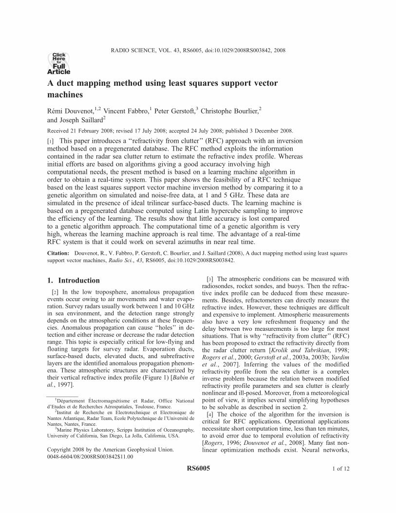
mal propagation. The refractivity is modified by temper-ature and/or humidity gradients. There are four identifiedtypes of duct [Turton et al., 1988] (Figure 1): curve a,evaporation duct; curve b, surface-based duct; curve c,elevated duct; and curve d, subrefractive layer. Elevatedducts are similar to surface-based ducts with a higherduct base. They are not taken into account in RFCbecause they have low influence on the power losses atthe sea level. Actually, the waves trapped into anelevated duct are bent at high altitude and reach thesea surface beyond the maximum radar range consideredfor RFC. The subrefractive layer is a rare event andmeasurements are lacking to be accurately characterized,hence it is not taken into account in this study.[9] The refractive conditions are considered constant

with the distance for the entire propagation path. Thishypothesis seems valid in open sea but could be a strongsimplification in coastal environment, where the meteo-rological conditions may highly vary [Kerr, 1987]. Adistance-varying refractive index could be introduced infurther work. Rogers [1996] shows that the RMS error inpropagation factor exceeds 6 dB or more after 30 mindue to temporal decorrelation. Thus, a practical RFCsystem has to update environment parameter estimatesmuch faster than 30 min. This calls for a simple range-independent model that can be estimated fast.

Figure 1. Modified refractivity profile and associated parameters for evaporation duct (curve a),surface-based duct (curve b), elevated duct (curve c), and subrefractive layer (curve d). Forevaporation duct and subrefractive layer, d is the duct height. For surface-based duct and elevatedduct, zb is the height of the duct base, Md is the M deficit into the duct, and zthick is the ductthickness.

RS6005 DOUVENOT ET AL.: A DUCT MAPPING METHOD USING LS-SV

2 of 12

RS6005

[10] The evaporation duct is a quasi-permanent eventabove the sea. It is due to a strong humidity gradient atthe sea surface, which causes a refractive index gradientas well. The worldwide mean of the duct height d,defined as the height above the sea mean level at whichdM/dz = 0 M unit/m (Figure 1, curve a), is about 10 m.The duct height sometimes reaches 30 m and exception-ally 40 m [Anderson, 1989; Patterson, 1992]. If the valueof d is considered as constant with the distance,performing an inversion in the case of an evaporationduct is not a hard problem because d is the onlyparameter to retrieve. A simple inversion method asgradient descent or quadratic regression could be used[Rogers et al., 2000].[11] On the contrary, the surface-based duct is less

frequent, but its effect on propagation is much stronger. Ithighly increases the radar range or creates detection‘‘holes.’’ Its occurrence is about 15% of the time world-wide but until 50% of the time in the Persian Gulf[Patterson, 1992]. It is often due to an advection move-ment of a relatively warm and dry air, which forms astrong negative gradient of modified refractivity. Thesurface-based duct is typically modeled as a trilinearprofile (Figure 1, curve b) [Gossard and Strauch, 1983],where zb is the height of the duct base, Md is the Mdeficit into the duct, and zthick is the duct thickness. Thefollowing limits for the duct parameters are chosen fromthe work of Gerstoft et al. [2003a]: zb varies from 0 to300 m, Md from 0 to 100 M unit, and zthick from 0 to100 m. The obtained profile is trilinear with slopediscontinuities at the basis and at the top of the duct. Acontinuous arctangent-shaped surface-based duct modelhas been proposed by Webster [1983] to avoid disconti-

nuities in the model. However, nor the trilinear modelneither the arctangent-shaped model are based on aphysical description and a model cannot be presentedas better than the other. Moreover, these two types ofducts have very close effects on the wave propagation(see Appendix A). We finally choose the trilinear model,which is simpler to use. Actually, the duct strength canbe linked to the parameters of the trilinear duct throughthe expression [Turton et al., 1988]

lmax !2Csbd %

!!!!!!

Md

p% zthick

3; #2$

where Csbd is a constant equal to 3.77 % 10"3 forsurface-based ducts and lmax is the maximum wave-length trapped into the duct in meter.[12] Evaporation ducts are modeled using one or two

parameters and are quite simple ducts to retrieve. TheLS-SVM RFC method has been applied on real data inthe presence of evaporation ducts [Douvenot et al.,2007]. Therefore, surface based ducts are considered totest and validate the feasibility of an RFC systemincluding the inversion method proposed in this paper.More complex and realistic profiles, as ‘‘double ducts’’composed of an evaporation duct and a surface-basedduct simultaneously, are to be studied in further works.

2.2. Sea Clutter Model

[13] In RFC technique, the propagation losses L areprocessed to determine the environmental parametersM = (zb, Md, zthick). In this paper, the refractiveconditions are determined from simulated propagationlosses. However, in operational conditions, only thepower PR(M) observed by the radar is available. Thereceived power has to be processed in order to isolatethe propagation losses. The received power can bewritten (from the radar equation) [Kerr, 1987, p. 473]

PR M# $ ! PEG2 4pl2

sL2 M# $; #3$

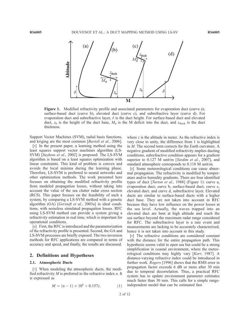
where the emitted power PE, the wavelength l, and theantenna gain G are known. Only the radar cross section(RCS) of the sea clutter s is needed to obtain thepropagation losses L from the received power. Now,the RCS s is the product of the illuminated area AI bythe Normalized RCS (NRCS) s0. The illuminated areacan be expressed as (Figure 2)

AI !1

2Rq3dB HORtc sec qg

" #

; #4$

where t is the radar pulse length, c is the velocity ofwave propagation, R is the distance from the radar tothe sea pixel, q3dBHOR is the horizontal antennaaperture, qg is the grazing angle, and sec denotes thesecant function. The range resolution of the radar is

Figure 2. The area illuminated by the radar (top) fromabove and (bottom) from the side. The parameter t is theradar pulse length, c is the velocity of wave propagation,R is the distance from the radar to the sea pixel, !3dBHOR

is the horizontal antenna aperture, !g is the grazing angle,and sec is the secant function.


3 of 12

RS6005

(1/2)tc [Kerr, 1987]. Note that AI is proportional to Rif qg is constant.[14] The problem is now to choose a model for the

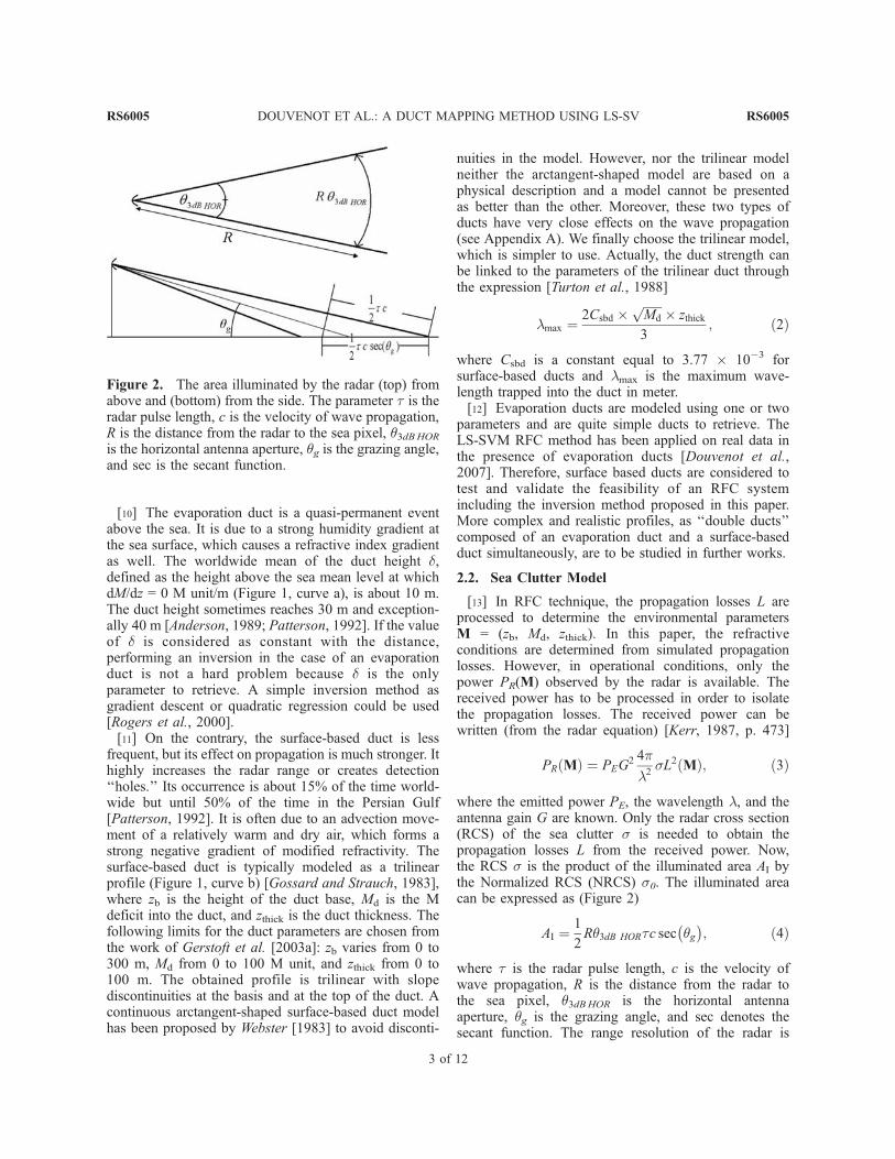
NRCS of the sea clutter s0. It depends on severalmeteorological parameters and on the grazing angle qg[Feng et al., 2005]. However, the grazing angle is almostconstant beyond the horizon in the presence of a range-independent evaporation duct [Paulus, 1990].[15] For instance, with an antenna at a height of 25 m,

the grazing angle hardly fluctuates beyond 10 km(Figure 3) for each refractivity condition. This result isobtained using ray tracing in heterogeneous and verti-cally stratified atmosphere [Paulus, 1990; Rogers et al.,2000]. The incident angle of the electromagnetic wave qgis determined at sea level. Considering the sea roughnessas uniform with the distance and the incident grazingangle of the trapped wave also as constant at the seasurface, s0 can be considered as constant beyond thehorizon. Hence the model s = Ct R, where Ct is aconstant, could be relevant. Note that these results areobtained for range-independent evaporation ducts. De-pendence with respect to the grazing angle [Ward et al.,2006] could be introduced for the study of complexrefractivity variations.[16] Once the propagation losses L are known, an

inversion algorithm is needed in order to retrieve theparameters of the modified refractivity profile.

3. Inversion Methods

[17] Retrieving the parameters of the ducts from thepropagation losses is a complex problem. Two different

inversion methods are presented in this paper. The first isa GA included in the SAGA code developed by Gerstoftet al. [2003a, 2003b]. The second, the LS-SVM, is alearning machine selected for its computational speedonce trained. This latter method is based on a pregen-erated and preprocessed database. As the main part of thecomputation is made prior to the operational use, theinversion using LS-SVM is real time.

3.1. Genetic Algorithm

[18] Genetic algorithms (GA) start with the selection ofa population of q member models. Models consist of bitstrings for each uncertain/unknown parameters (parame-ters are, thus, discretized in GA, in contrast to SimulatedAnnealing methods, which usually work with continuousvariables).[19] The ‘‘fitness’’ of each member is the value of the

objective function for the particular model. On the basisof the fitness of the members, ‘‘parents’’ are selected andthrough a randomization, a set of ‘‘children’’ is pro-duced. These children replace the least fit of the originalpopulation and the process iterates to develop an overallfitter population. The formation of child models isperformed through the application of operators to theparents.[20] Figure 4 shows the GA principle. Each child

population Pi+1 is processed in three steps: first, themore likely ‘‘parents’’ are selected in the parent popula-tion Pi. Then, crossover uses a part of the string corres-ponding to a parameter from one parent and supplementsit with a part of the string for the same parameter fromthe other parent. The operation is applied individually toevery parameter string (multipoint crossover), resultingin all-direction parameter perturbations.[21] Mutation follows crossover and changes bit values

in parameter strings in a random fashion. Bit changesoccur with a low probability (usually 0.05). The smallchanges imposed on the new generation through theoccasional bit changes assist the optimization processto escape from local minima. These three steps areapplied on each population to obtain a final populationcontaining an overall fitter population Pk. A more de-tailed description of genetic algorithms and their appli-cation to parameter estimation is given by Gerstoft[1994].

3.2. LS-SVM

[22] In the late 1990s, Suykens and Vandewalle [1999]developed LS-SVM from Vapnik’s work on supportvector machines (SVM) [Vapnik and Lerner, 1963;Vapnik and Chervonenkis, 1964; Vapnik, 1995]. Thisspecial case (quadratic loss function) simplifies theSVM theory formulation as exposed by Smola andScholkopf [1998]. Moreover, the authors made greatefforts to unify the theories of LS-SVM, neural net-

Figure 3. Reflection angle with respect to the distancein the presence of an evaporation duct for d = 2.5, 10,and 20 m. Antenna is at a height of 25 m.


4 of 12

RS6005

works, optimization, and Gaussian processes. FollowingSuykens et al. [2002], the theory is outlined below.[23] LS-SVM is a training process. The aim of

the training process is to obtain an approximationof the nonlinear function f with respect to the vector ofthe propagation losses L at different ranges. The vectorof the duct parameters M is the output: M = f(L).[24] Figure 5 displays the process to generate the N

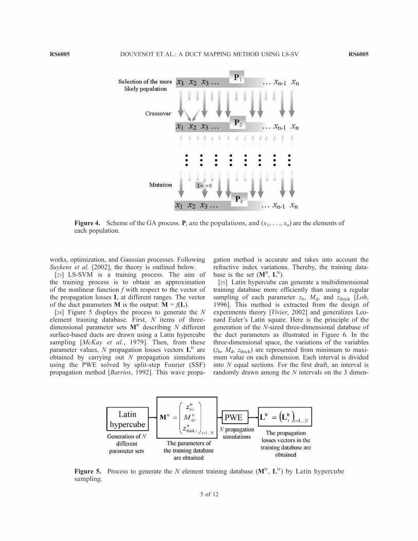
element training database. First, N items of three-dimensional parameter sets Mtr describing N differentsurface-based ducts are drawn using a Latin hypercubesampling [McKay et al., 1979]. Then, from theseparameter values, N propagation losses vectors Ltr areobtained by carrying out N propagation simulationsusing the PWE solved by split-step Fourier (SSF)propagation method [Barrios, 1992]. This wave propa-

gation method is accurate and takes into account therefractive index variations. Thereby, the training data-base is the set (Mtr, Ltr).[25] Latin hypercube can generate a multidimensional

training database more efficiently than using a regularsampling of each parameter zb, Md, and zthick [Loh,1996]. This method is extracted from the design ofexperiments theory [Vivier, 2002] and generalizes Leo-nard Euler’s Latin square. Here is the principle of thegeneration of the N-sized three-dimensional database ofthe duct parameters as illustrated in Figure 6. In thethree-dimensional space, the variations of the variables(zb, Md, zthick) are represented from minimum to maxi-mum value on each dimension. Each interval is dividedinto N equal sections. For the first draft, an interval israndomly drawn among the N intervals on the 3 dimen-

Figure 5. Process to generate the N element training database (Mtr, Ltr) by Latin hypercubesampling.

Figure 4. Scheme of the GA process. Pi are the populations, and (x1, . . ., xn) are the elements ofeach population.


5 of 12

RS6005

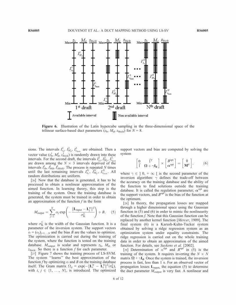
sions. The intervals Izb1 , IMd

1 , Izthick1 are obtained. Then a

vector value (zb1, Md

1, zthick1 ) is randomly drawn into these

intervals. For the second draft, the intervals Izb2 , IMd

2 , Izthick2

are drawn among the N % 3 intervals deprived of theintervals Izb

1 , IMd1 , Izthick

1 . The process is repeated N timesuntil the last remaining intervals Izb

N , IMd

N , IzthickN . All

random distributions are uniform.[26] Now that the database is generated, it has to be

processed to obtain a nonlinear approximation of theaimed function. In learning theory, this step is thetraining of the system. Once the training database isgenerated, the system must be trained in order to obtainan approximation of the function f in the form

Moutput !X

N

j!1

aj exp "kLinput " Ltr

j k2

s2K

!

& B; #5$

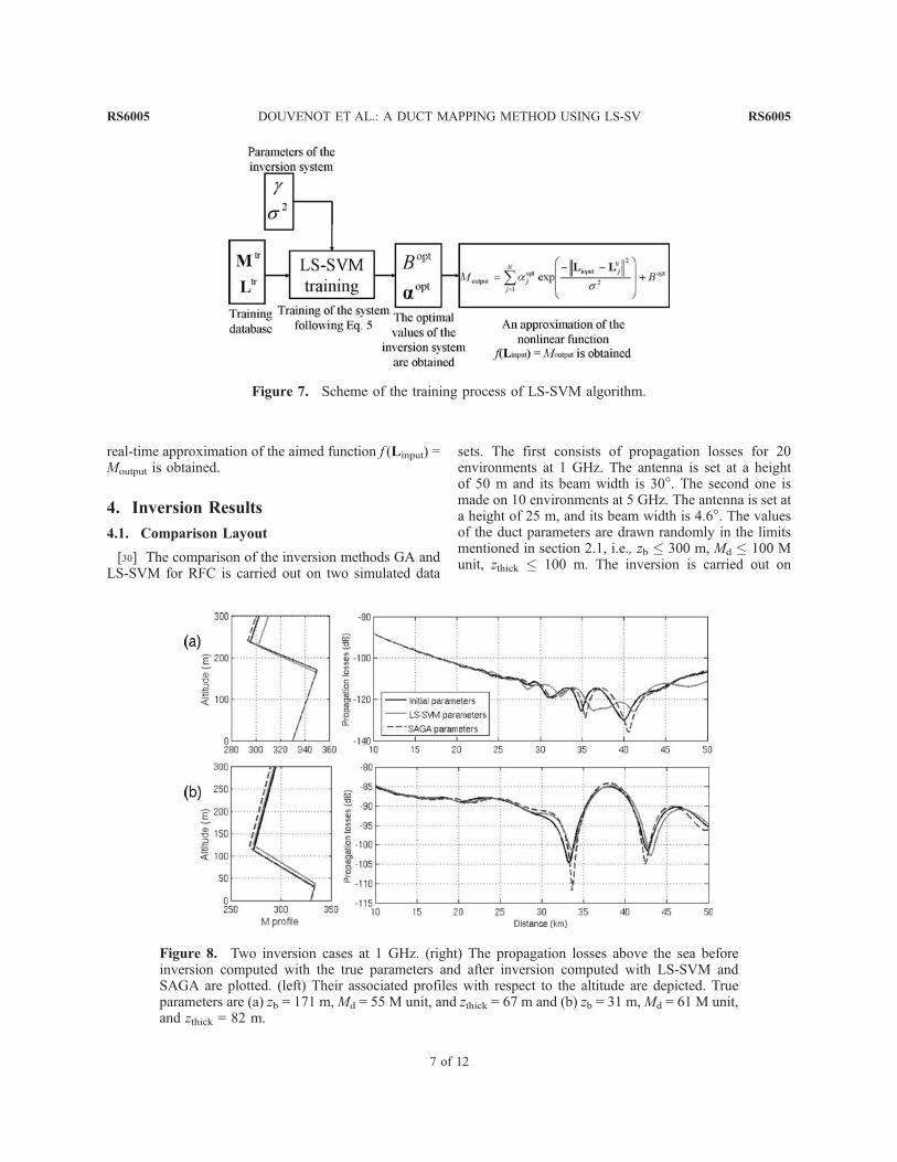
where sK2 is the width of the Gaussian function. It is aparameter of the inversion system. The support vectorsa = (aj)j=1. . .N and the bias B are the values to optimize.The optimization is carried out during the training ofthe system, where the function is tested on the trainingdatabase. Moutput is scalar and represents zb, Md, orzthick. So there is a function f for each parameter.[27] Figure 7 shows the training process of LS-SVM.

The system ‘‘learns’’ the best approximation of thefunction f by optimizing a and B on the training databaseitself. The Gram matrix Wij = exp("kLi

tr " Ljtrk2/sK2 ),

with i, j 2 {1, . . ., N}, is introduced. The optimized

support vectors and bias are computed by solving thesystem

0 ~1T

~1 W& gId

$ %

% Bopt

aopt

$ %

! 0Mtr

$ %

; #6$

where g 2 ] 0, + 1 [ is the second parameter of theinversion algorithm: g defines the trade-off betweenthe accuracy on the training database and the ability ofthe function to find solutions outside the trainingdatabase. It is called the regulation parameter; aopt arethe support vectors, and Bopt is the bias of the function atthe optimum.[28] In theory, the propagation losses are mapped

through a higher dimensional space using the Gaussianfunction in (5) and (6) in order to mimic the nonlinearityof the function f. Note that this Gaussian function can bereplaced by another kernel function [Mercer, 1909]. Thefinal system (6) is a Karush-Kuhn-Tucker systemobtained by solving a ridge regression system as anoptimization system under equality constraints. Theridge regression is carried out on the whole trainingdata in order to obtain an approximation of the aimedfunction. For details, see Suykens et al. [2002].[29] Determination of aopt and Bopt in (5) is the

training of the system. It requires inverting the N % Nmatrix W + gId. Once the system is trained, the inversionprocess is fast, less than 1 s. For an observed vector ofpropagation losses Linput, the equation (5) to determinethe duct parameter Moutput is very fast. A nonlinear and

Figure 6. Illustration of the Latin hypercube sampling in the three-dimensional space of thetrilinear surface-based duct parameters (zb, Md, zthick) for N = 8.


6 of 12

RS6005

real-time approximation of the aimed function f (Linput) =Moutput is obtained.

4. Inversion Results

4.1. Comparison Layout

[30] The comparison of the inversion methods GA andLS-SVM for RFC is carried out on two simulated data

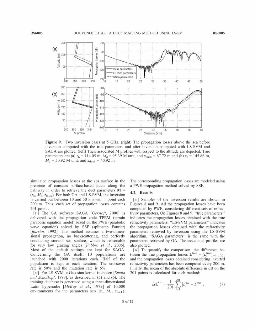
sets. The first consists of propagation losses for 20environments at 1 GHz. The antenna is set at a heightof 50 m and its beam width is 30!. The second one ismade on 10 environments at 5 GHz. The antenna is set ata height of 25 m, and its beam width is 4.6!. The valuesof the duct parameters are drawn randomly in the limitsmentioned in section 2.1, i.e., zb ' 300 m, Md ' 100 Munit, zthick ' 100 m. The inversion is carried out on

Figure 7. Scheme of the training process of LS-SVM algorithm.

Figure 8. Two inversion cases at 1 GHz. (right) The propagation losses above the sea beforeinversion computed with the true parameters and after inversion computed with LS-SVM andSAGA are plotted. (left) Their associated profiles with respect to the altitude are depicted. Trueparameters are (a) zb = 171 m,Md = 55 M unit, and zthick = 67 m and (b) zb = 31 m,Md = 61 M unit,and zthick = 82 m.


7 of 12

RS6005

simulated propagation losses at the sea surface in thepresence of constant surface-based ducts along thepathway in order to retrieve the duct parameters M =(zb, Md, zthick). For both GA and LS-SVM, the inversionis carried out between 10 and 50 km with 1 point each200 m. Thus, each set of propagation losses contains201 points.[31] The GA software SAGA [Gerstoft, 2006] is

delivered with the propagation code TPEM (terrainparabolic equation model) based on the PWE (parabolicwave equation) solved by SSF (split-step Fourier)[Barrios, 1992]. This method assumes a two-dimen-sional propagation, no backscattering, and perfectlyconducting smooth sea surface, which is reasonablefor very low grazing angles [Fabbro et al., 2006].Most of the default settings are kept for SAGA.Concerning the GA itself, 10 populations arelaunched with 2000 iterations each. Half of thepopulation is kept at each iteration. The crossoverrate is 50% and the mutation rate is 5%.[32] For LS-SVM, a Gaussian kernel is chosen [Smola

and Scholkopf, 1998], as described in (5) and (6). Thetraining database is generated using a three-dimensionalLatin hypercube [McKay et al., 1979] of 10,000environments for the parameters sets (zb, Md, zthick).

The corresponding propagation losses are modeled usinga PWE propagation method solved by SSF.

4.2. Results

[33] Samples of the inversion results are shown inFigures 8 and 9. All the propagation losses have beencomputed by PWE, considering different sets of refrac-tivity parameters. On Figures 8 and 9, ‘‘true parameters’’indicates the propagation losses obtained with the truerefractivity parameters. ‘‘LS-SVM parameters’’ indicatesthe propagation losses obtained with the refractivityparameters retrieved by inversion using the LS-SVMalgorithm. ‘‘SAGA parameters’’ is the same with theparameters retrieved by GA. The associated profiles arealso plotted.[34] To quantify the comparison, the difference be-

tween the true propagation losses Ltrue = (Litrue)i=1. . .201

and the propagation losses obtained considering invertedrefractivity parameters has been computed every 200 m.Finally, the mean of the absolute difference in dB on the201 points is calculated for each method:

DLinv ! 1

201

X

201

i!1

Linvi " Ltruei

&

&

&

&; #7$

Figure 9. Two inversion cases at 5 GHz. (right) The propagation losses above the sea beforeinversion computed with the true parameters and after inversion computed with LS-SVM andSAGA are plotted. (left) Their associated M profiles with respect to the altitude are depicted. Trueparameters are (a) zb = 114.05 m, Md = 95.39 M unit, and zthick = 67.72 m and (b) zb = 145.86 m,Md = 50.92 M unit, and zthick = 40.92 m.


8 of 12

RS6005

where the superscript ‘‘inv’’ is the name of the inversionmethod (LS-SVM or GA). This result is finally averagedon all the tested cases to get a global error estimationDLmean

inv .[35] The results of LS-SVM and GA inversions are

summarized as follows: (1) at 1 GHz, DLmeanLSSVM =

2.38 dB and DLmeanGA (mean on 20 cases); and (2) at

5 GHz, DLmeanLSSVM = 2.71 dB and DLmean

GA = 1.54 dB(mean on 10 cases).[36] The two algorithms are fundamentally different

and this is observed in the results. GA is more accuratethan LS-SVM, but GA uses significantly more CPUtime. The mean of the computation time for the GA isTmeanGA ( 90 min at 1 GHz and Tmean

GA ( 1100 min at5 GHz. On the same computer, for the LS-SVMalgorithm, Tmean

LSSVM ' 0.2 s for both frequencies.Actually, as shown in section 3.2, LS-SVM only requiresthe calculus of the kernel function, whereas the GArequires a propagation computation, longer at 5 GHzthan at 1 GHz, for each forward model. For LS-SVMapproach, all the propagation computations have beenpreprocessed during the training step.[37] Event though the GA gives more accurate results,

the LS-SVM gives a good idea of the wave propagationand of the atmospheric duct as shown in Figure 8 (for1 GHz) and Figure 9 (5 GHz). The one-way propagationlosses above the sea are shown for the true surface-basedduct parameters and for the parameters retrieved byinversion with the LS-SVM algorithm and with theGA. Then the associated refractive profiles are plotted.The two cases are shown at each frequency. The prop-agation losses obtained with the GA parameters fit theoriginal ones. However, apart from small discrepancies,the LS-SVM curve follows the original one. Moreover,the ducts retrieved by LS-SVM are close to the originalones. Such accuracy might be sufficient to characterizethe environment effect on propagation in order topredict trapping phenomenon and to detect shadowzones in the radar cover as the duct itself is wellapproximated by LS-SVM.

5. Summary and Conclusion

[38] In this paper, the feasibility of a RFC system usinga learning machine has been shown on simulated data.The simplifying hypotheses have first been explained,then the method has been compared to a GA RFC systemon noiseless simulated data. The results show a minorreduction in accuracy but a great improvement in com-putation time. Our system is especially interesting inhigher frequencies, around 5 GHz, when the computationtime of the GA-type RFC systems are very slow. Themain interest of the LS-SVM learning machine is tomake all the main calculations before the inversion is

started. Then the obtained RFC system could work inreal time.[39] The LS-SVM inversion method is not as precise as

the GA one. Yet, the system gives a good idea of theelectromagnetic wave behavior and of the refractive indexprofile. Both methods are less precise at 5 GHz as thewave is more sensitive to refractive index variations.[40] There are several ways to improve the RFC using

learning machine: the first means is to improve the veryinversion algorithm. An interesting way is to find a fitterkernel than the Gaussian kernel to the RFC problem.However, creating a kernel for a specific problem is adifficult task. Another possible improvement is theintroduction of a correlation between the differentdimensions of the duct during the inversion. The use ofa multitask learning algorithm [Argyriou et al., 2006]could improve the inversion by inverting the three ductparameters at once. To improve the inversion, thismethod could also be hybridized with a GA-typeinversion: the LS-SVM inversion could give a firstapproximation of the duct parameters, and then the GAcould refine the inversion. Therefore, the inversion couldhave the accuracy of GAwith a lower computation time.[41] Another way to improve RFC using a learning

machine is to optimize the training database. Indeed, asLS-SVM is a learning machine, the generation of thetraining database is critical for the efficiency of thealgorithm. To generate an efficient training database,one must describe at best all the possible cases. Thus,large and precise meteorological data could permit torefine the values of the parameters describing the duct inthe training database. The more precise the database, themore likely the inversion is to succeed. Moreover, thechoice of the sampling method is decisive. A samplingmethod better than Latin hypercube sampling could beapplied for RFC.[42] If the LS-SVM inversion is not precise enough to

perfectly retrieve the refractivity profile, the advantage ofthis method is the real-time working. In operationalconditions, the radar can observe several azimuths atseveral times. The obtained results could be smoothedover time and space in order to correlate the results.Having data at several frequencies or several elevationangles could also be useful.

Appendix A

[43] The debate of surface-based duct modeling is stillopen. One point of interest is the discontinuities in thevertical profile. To discuss the choice of a trilinearsurface-based duct profile, which implies discontinuities,a comparison is carried out with a continuous arctangent-shaped profile, as advised by Webster [1983]. This


9 of 12

RS6005

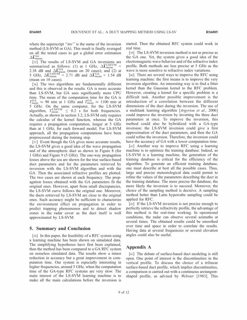
comparison has been made at 2.84 GHz with an antennaat a height of 30.78 m.[44] Figure A1 (left) represents the modified refractiv-

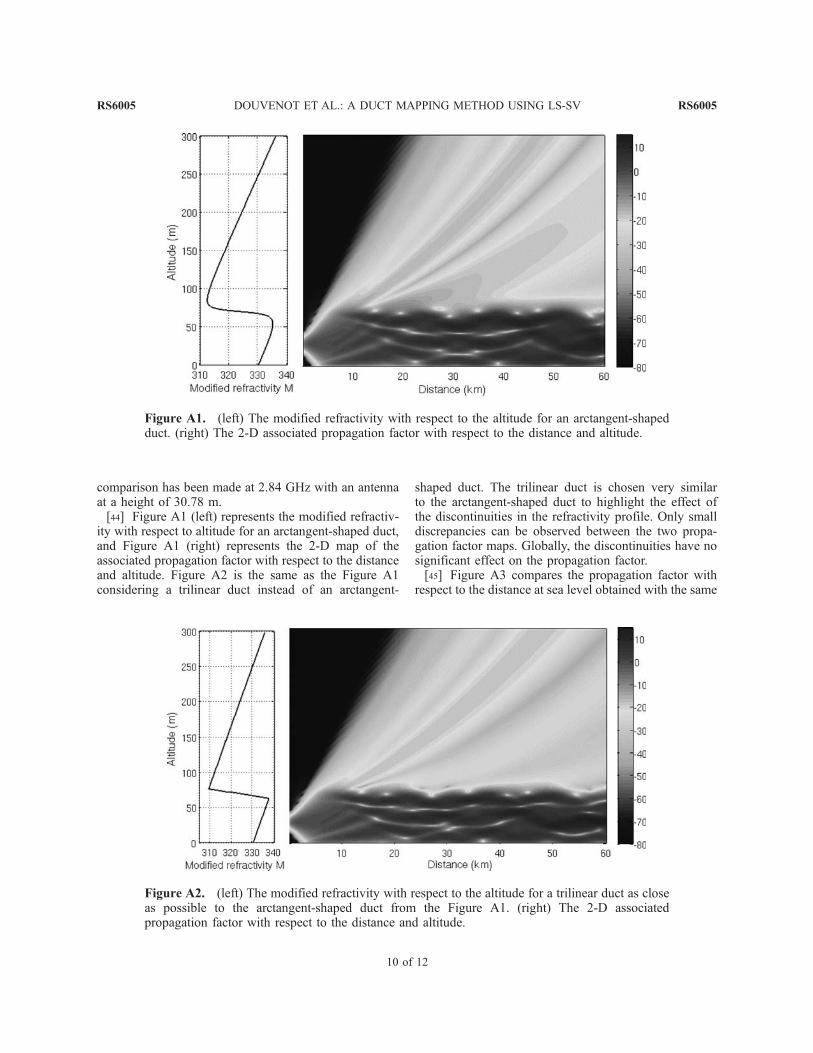
ity with respect to altitude for an arctangent-shaped duct,and Figure A1 (right) represents the 2-D map of theassociated propagation factor with respect to the distanceand altitude. Figure A2 is the same as the Figure A1considering a trilinear duct instead of an arctangent-

shaped duct. The trilinear duct is chosen very similarto the arctangent-shaped duct to highlight the effect ofthe discontinuities in the refractivity profile. Only smalldiscrepancies can be observed between the two propa-gation factor maps. Globally, the discontinuities have nosignificant effect on the propagation factor.[45] Figure A3 compares the propagation factor with

respect to the distance at sea level obtained with the same

Figure A1. (left) The modified refractivity with respect to the altitude for an arctangent-shapedduct. (right) The 2-D associated propagation factor with respect to the distance and altitude.

Figure A2. (left) The modified refractivity with respect to the altitude for a trilinear duct as closeas possible to the arctangent-shaped duct from the Figure A1. (right) The 2-D associatedpropagation factor with respect to the distance and altitude.


10 of 12

RS6005

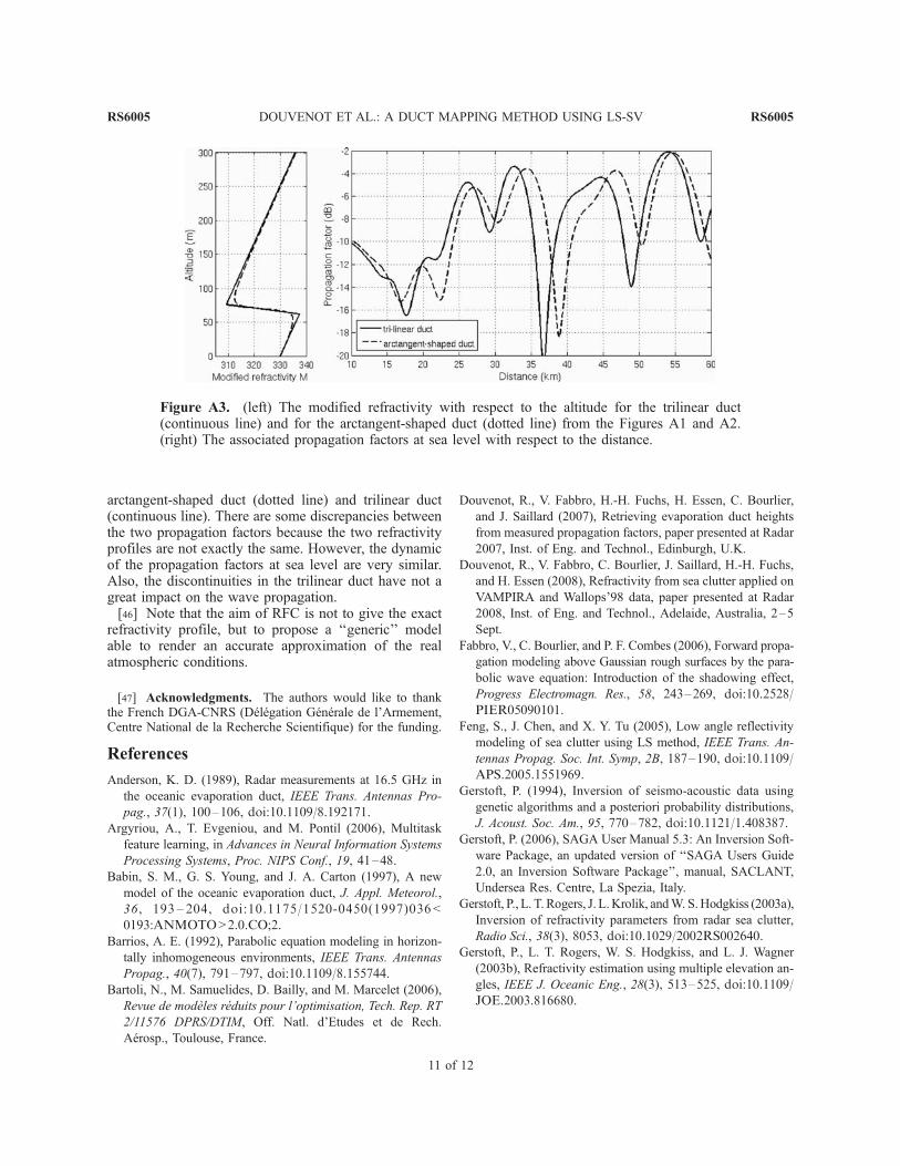
arctangent-shaped duct (dotted line) and trilinear duct(continuous line). There are some discrepancies betweenthe two propagation factors because the two refractivityprofiles are not exactly the same. However, the dynamicof the propagation factors at sea level are very similar.Also, the discontinuities in the trilinear duct have not agreat impact on the wave propagation.[46] Note that the aim of RFC is not to give the exact

refractivity profile, but to propose a ‘‘generic’’ modelable to render an accurate approximation of the realatmospheric conditions.

[47] Acknowledgments. The authors would like to thankthe French DGA-CNRS (Delegation Generale de l’Armement,Centre National de la Recherche Scientifique) for the funding.

References

Anderson, K. D. (1989), Radar measurements at 16.5 GHz inthe oceanic evaporation duct, IEEE Trans. Antennas Pro-pag., 37(1), 100–106, doi:10.1109/8.192171.

Argyriou, A., T. Evgeniou, and M. Pontil (2006), Multitaskfeature learning, in Advances in Neural Information SystemsProcessing Systems, Proc. NIPS Conf., 19, 41–48.

Babin, S. M., G. S. Young, and J. A. Carton (1997), A newmodel of the oceanic evaporation duct, J. Appl. Meteorol.,36, 193 – 204, doi:10.1175/1520-0450(1997)036<0193:ANMOTO>2.0.CO;2.

Barrios, A. E. (1992), Parabolic equation modeling in horizon-tally inhomogeneous environments, IEEE Trans. AntennasPropag., 40(7), 791–797, doi:10.1109/8.155744.

Bartoli, N., M. Samuelides, D. Bailly, and M. Marcelet (2006),Revue de modeles reduits pour l’optimisation, Tech. Rep. RT2/11576 DPRS/DTIM, Off. Natl. d’Etudes et de Rech.Aerosp., Toulouse, France.

Douvenot, R., V. Fabbro, H.-H. Fuchs, H. Essen, C. Bourlier,and J. Saillard (2007), Retrieving evaporation duct heightsfrom measured propagation factors, paper presented at Radar2007, Inst. of Eng. and Technol., Edinburgh, U.K.

Douvenot, R., V. Fabbro, C. Bourlier, J. Saillard, H.-H. Fuchs,and H. Essen (2008), Refractivity from sea clutter applied onVAMPIRA and Wallops’98 data, paper presented at Radar2008, Inst. of Eng. and Technol., Adelaide, Australia, 2–5Sept.

Fabbro, V., C. Bourlier, and P. F. Combes (2006), Forward propa-gation modeling above Gaussian rough surfaces by the para-bolic wave equation: Introduction of the shadowing effect,Progress Electromagn. Res., 58, 243–269, doi:10.2528/PIER05090101.

Feng, S., J. Chen, and X. Y. Tu (2005), Low angle reflectivitymodeling of sea clutter using LS method, IEEE Trans. An-

tennas Propag. Soc. Int. Symp, 2B, 187–190, doi:10.1109/APS.2005.1551969.

Gerstoft, P. (1994), Inversion of seismo-acoustic data usinggenetic algorithms and a posteriori probability distributions,J. Acoust. Soc. Am., 95, 770–782, doi:10.1121/1.408387.

Gerstoft, P. (2006), SAGA User Manual 5.3: An Inversion Soft-ware Package, an updated version of ‘‘SAGA Users Guide2.0, an Inversion Software Package’’, manual, SACLANT,Undersea Res. Centre, La Spezia, Italy.

Gerstoft, P., L. T. Rogers, J. L.Krolik, andW. S.Hodgkiss (2003a),Inversion of refractivity parameters from radar sea clutter,Radio Sci., 38(3), 8053, doi:10.1029/2002RS002640.

Gerstoft, P., L. T. Rogers, W. S. Hodgkiss, and L. J. Wagner(2003b), Refractivity estimation using multiple elevation an-gles, IEEE J. Oceanic Eng., 28(3), 513–525, doi:10.1109/JOE.2003.816680.

Figure A3. (left) The modified refractivity with respect to the altitude for the trilinear duct(continuous line) and for the arctangent-shaped duct (dotted line) from the Figures A1 and A2.(right) The associated propagation factors at sea level with respect to the distance.


11 of 12

RS6005

Gossard, E. E., and R. G. Strauch (1983), Radar Observation of

Clear Air and Clouds, Elsevier Sci., Amsterdam.Kerr, D. E. (1987), Propagation of Short Radio Waves, IEE

Electromagn. Waves Ser., vol. 24, Peter Peregrinus, London.Krolik, J. L., and J. Tabrikian (1998), Tropospheric refractivity

estimation using radar clutter from the sea surface, in Pro-ceedings of the 1997 Battlespace Atmospherics Conference,

SPAWAR Syst. Command Tech. Rep. 2989, pp. 635–642,Space and Nav. Warfare Syst. Command Cent., San Diego,Calif.

Loh, W.-L. (1996), On Latin hypercube sampling, Ann. Stat.,24(5), 2058–2080, doi:10.1214/aos/1069362310.

McKay, M. D., W. J. Conover, and R. J. Beckman (1979), Acomparison of three methods for selecting values of inputvariables in the analysis of output from a computer code,Technometrics, 21(2), 239–245.

Mercer, J. (1909), Functions of positive and negative type andtheir connection with the theory of integral equations, Phi-los. Trans. R. Soc. London, 209, 415–446, doi:10.1098/rsta.1909.0016.

Patterson, W. (1992), Ducting climatology summary, report,Space and Nav. Warfare Syst. Cent., San Diego, Calif.

Paulus, R. (1990), Evaporation duct effects on sea clutter, IEEETrans. Antennas Propag., 38(11), 1765–1771, doi:10.1109/8.102737.

Rogers, L. T. (1996), Effects of the variability of atmosphericrefractivity on propagation estimates, IEEE Trans. Antennas

Propag., 44(4), 460–465, doi:10.1109/8.489297.Rogers, L. T., C. P. Hattan, and J. K. Stapleton (2000), Estimat-

ing evaporation duct heights from radar sea clutter, RadioSci., 35(4), 955–966, doi:10.1029/1999RS002275.

Smola, A. J., and B. Scholkopf (1998), A tutorial on supportvector regression, NeuroCOLT Tech. Rep. NC-TR-98-030,R. Holloway Coll., Univ. of London, London, U.K.

Suykens, J. A. K., and J. Vandewalle (1999), Least squaressupport vector machine classifier, Neural Processes Lett.,9(3), 293–300, doi:10.1023/A:1018628609742.

Suykens, J. A. K., Van T. Gestel, De J. Brabanter, B. De Moor,and J. Vandewalle (2002), Least Squares Support VectorMachines, World Sci., Singapore.

Turton, J. D., D. A. Bennetts, and S. F. G. Farmer (1988), Anintroduction to radio ducting, Meteorol. Mag., 117, 245–254.

Vapnik, V. (1995), The Nature of Statistical Learning Theory,Springer, New York.

Vapnik, V., and A. Chervonenkis (1964), A note on one class ofperceptions, Autom. Remote Control, 25, 821–837.

Vapnik, V., and A. Lerner (1963), Pattern recognition usinggeneralized portrait method, Autom. Remote Control, 24,774–780.

Vivier, S. (2002), Strategies d’optimisation par la methode desplans d’experience et application aux dispositifs electrotech-niques modelises par elements finis, Ph.D. thesis, EcoleCent. Lille and Univ. des Sci. et Technol., Lille, France.

Ward, K. D., R. J. A. Tough, and S. Watts (2006), Sea Clutter:Scattering, the K Distribution and Radar Performance, TheInstitution of Engineering Technology, London, UK.

Webster, A. R. (1983), Angles-of-arrival and delay times onterrestrial line-of-sight microwave links, IEEE Trans. Anten-nas Propag., 31(1), 12–17, doi:10.1109/TAP.1983.1142976.

Yardim, C., P. Gerstoft, and W. S. Hodgkiss (2007), Statisticalmaritime radar duct estimation using hybrid geneticalgorithm–Markov chain Monte Carlo method, Radio Sci.,42, RS3014, doi:10.1029/2006RS003561.

""""""""""""C. Bourlier and J. Saillard, Institut de Recherche en

Electrotechnique et Electronique de Nantes Atlantique, RadarTeam, Ecole Polytechnique de l’Universite de Nantes, RueChristian Pauc, La Chantrerie, BP 50609, 44306 Nantes,France.

R. Douvenot and V. Fabbro, Departement Electromagne-tisme et Radar, BP 4025, ONERA, 2 avenue Edouard Belin,F-31055 Toulouse CEDEX 4, France. ([email protected])

P. Gerstoft, Marine Physics Laboratory, Scripps Institutionof Oceanography, University of California, San Diego,MC0238, 9500 Gillman Drive, La Jolla, CA 92093-0238,USA.


12 of 12

RS6005

a duct mapping method using least squares support vector...

Documents