a customer management dilemma: when is it profitable to...
TRANSCRIPT
A Customer Management Dilemma:
When Is It Profitable to Reward Existing Customers?
Jiwoong Shin and K. Sudhir*
Yale University
September 2009
* The authors thank the editor, the area editor, and the four anonymous reviewers for their very constructive and detailed comments during the review process. The authors are grateful to Drew Fudenberg, Duncan Simester, J. Miguel Villas-Boas, and Birger Wernerfelt for their helpful comments. They also thank seminar participants at Duke, Korea University, Stanford, UCLA, University of Chicago, University of Toronto, and Yale, as well as participants in the NEMC conference at MIT and the SICS conference at UC Berkeley for their comments and suggestions. The authors contributed equally and their names are listed in alphabetical order. Correspondence: 135 Prospect St., P.O. Box 208200, New Haven, CT 06520, email: [email protected], [email protected]
A Customer Management Dilemma:
When Is It Profitable to Reward Existing Customers?
Abstract
This study attempts to answer a basic customer management dilemma facing firms: When should
the firm use behavior-based pricing (BBP) to discriminate between its own and competitors’
customers in a competitive market? If BBP is profitable, when should the firm offer a lower
price to its own customers rather than to the competitor's customers? This analysis considers two
features of customer behavior hitherto ignored in BBP literature: heterogeneity in customer value
and changing preference (i.e., customer preferences are correlated but not fixed over time). In a
model where both consumers and competing firms are forward looking, we identify conditions
when it is optimal to reward the firm’s own or competitor’s customers and when BBP increases
or decreases profits. To the best of our knowledge, we are the first to identify conditions in
which (1) it is optimal to reward one’s own customers under symmetric competition and (2) BBP
can increase profits with fully strategic and forward-looking consumers.
Key Words: Behavior-based pricing, Customer heterogeneity, Stochastic Preferences, Forward-
looking customers, Forward-looking firms, Customer relationship management,
Competitive strategy, Game theory.
1
1. Introduction
Over the past two decades, firms have made massive investments of their organizational
resources (human, technical, and financial) into building information infrastructures that store
and analyze data about customer purchase behavior. Armed with such data, firms can pursue
detailed micro-segmentation and customer management strategies. A routinely used strategy is
behavior-based pricing (BBP), such that firms offer different prices to different customers based
on their past purchase behavior.1 However, firms differ in whether they offer a lower price to
their own customers or competitors’ customers. Catalog retailers for items such as apparel
typically send special discount “value” catalogs to existing customers, whereas magazines and
software firms often offer discounts to buyers of competing products in the form of lowered
introductory prices. Would it be more profitable for a magazine to offer a better price for a
subscription renewal as opposed to a new subscription? Should a wireless carrier offer lower
rates to its high-volume customers who use more minutes or to its new customers? Should a
hotel, airline, or retailer offer better rates for high value, loyalty card members or to new
customers it seeks to acquire? This paper answers a basic customer management dilemma for
firms practicing BBP: When should a firm use BBP to discriminate between its own and
competitors’ customers in a competitive market? If BBP is profitable, when should the firm offer
the lower price to its own customers rather than competitor's customers?
Although this customer management dilemma is ubiquitous across industries, little consensus
exists about the correct answers to these questions. The academic literature differs sharply from
the practitioner intuition on these questions. O’Brien and Jones (1995, p. 76) epitomize the
conventional wisdom of many practitioners: “to maximize loyalty and profitability, a company
1 The literature variously refers to it as behavior-based price discrimination (Fudenberg and Tirole 2000) or pricing with customer recognition (Villas-Boas 1999, 2004).
2
must give its best value to its best customers. As a result, they will then become even more loyal
and profitable” (emphasis added). Essentially, practitioners argue that rewarding own customers
leads to a virtuous cycle: The firm rewards its current customers with better value propositions,
which makes it optimal for those customers to deepen their relationship with the firm, which
ultimately increases firm profitability (Peppers and Rogers 2004).
But academic literature is skeptical of this conventional wisdom. In most existing models of
BBP, the optimal choice is not to offer current customers a lower price. When the firm can price
discriminate on the basis of consumers’ past purchase behavior, it should charge higher prices to
existing customers, who already have revealed their higher willingness to pay for the product
(otherwise, they would not have purchased from it), relative to competitor’s customers. That is,
customers’ past purchases reveal their relative preference for each firm. Further, if consumers
recognize the possibility that they will be penalized in future, they can alter their behavior to
reduce the ability of firms to infer their true preferences. Such strategic behavior by consumers
and increased competition to poach others’ customers may make BBP unprofitable. Fudenberg
and Villas-Boas’s (2006, p. 2) succinct summary of existing literature on BBP notes: “the seller
may be better off if it can commit to ignore information about buyer’s past decisions … more
information will lead to more intense competition between firms.” The overall lesson is that
BBP cannot be profitable if both consumers and firms are rational and forward looking;
furthermore, it is never optimal to reward one's own customers.
In this paper, we resolve this discrepancy between theoretical predictions and practitioner
intuitions by incorporating two simple but important features of customer behavior into our
analytical model. Our results nest these two viewpoints and identify conditions in which either
3
practitioner intuition or current theoretical results hold, even when both consumers and firms are
strategic and forward-looking. We now describe the two key features that we add.
1.1. Customer Value Heterogeneity
Not all customers are equally valuable to firms. Some purchase more than others or contribute
more to a firm’s profits. Widespread empirical support in various categories confirms the 80/20
rule, that is, the idea that a small proportion of customers contributes to most of the purchases
and profit in a category (Schmittlein et al. 1993). Such customer heterogeneity is critical for
capturing the practitioner notion of a “best” customer – a feature generally does not appear in
current analytical models.
Modeling customer heterogeneity in purchase quantity also allows firms to gain a new
dimension of information about consumers from their purchase history data. In addition to the
usual "whom they bought from" data, which provide horizontal information about the relative
preferences of consumers, data pertaining to "how much they bought" provide vertical
information about the relative importance of consumers to the firm.
Vertical information about quantity not only provides additional information to firms but also
generates an information asymmetry among otherwise symmetric firms. With these data, a firm
can identify the “best customers” only among its own customers, but not among its competitor’s
customers. Although the firm knows there are a mix of high and low volume customers among
its competitor’s customers, it cannot know the exact identity of who is who. Existing models
assume that all customers buy just one unit of the product and the market is fully covered, which
implies that if a consumer does not buy from one firm, it must have bought from the other and,
therefore, there is no information advantage about one's own customers. That is, existing models
abstract away from a major reason that firms invest in customer relationship management (CRM)
4
in practice: to obtain an information advantage over competitors about existing customers. This
information asymmetry emerges as critical for obtaining more complete insights into BBP.
1.2. Stochastic Preferences
We also recognize that consumers’ preferences can be stochastic. Consumer preference for a
product may change across purchase occasions, independent of the marketing mix or pricing,
because their needs or wants depend on the specific purchase situation, which changes over time
(Wernerfelt 1994). This is relevant in many choice contexts. For example, for store choice,
consumers’ preferred geographic locations likely vary across time; a customer may generally
prefer Lowe’s for purchasing home improvement products because a store is closer to her home
and offers superior quality offerings. However, she may visit the Home Depot store that is on her
way home from work. A similar logic may apply to consumers’ choices of hotels; even if a
customer prefers Marriott in general, he may find that a Sheraton satisfies his needs better on a
particular trip because of its proximity to a conference venue.2
Previous research in BBP (e.g., Caminal and Matutues 1990, Fudenberg and Tirole 2000)
recognizes the possibility of stochastic preference, but only for the extreme case in which
customers’ preferences are completely independent over time. Although the independence
assumption makes the analysis tractable, it is not innocuous in a customer management context.
With completely independent preferences, customers’ past purchases are of no use in predicting
future purchases. For past purchase information to be valuable to firms in future price setting
efforts, those preferences must be correlated across time. Our formulation of stochastic
preferences will accommodate such correlation in preferences across time, a characteristic of
most real world markets.
2 It is important to note that we are not assuming that consumer choice changes over time. Consumers’ purchase choice is still endogenous decision. For example, even if the Sheraton is preferable because of its proximity to a conference venue, a consumer may still stay in Marriott if Marriott offers a special deal or some other incentive.
5
With these two features included, we identify conditions in which (1) behavior-based pricing
is profitable in a competitive market, even when firms and consumers are strategic and forward
looking, and (2) firms should offer lower prices to their own best customers or to competitor’s
customers. We find that either sufficiently high heterogeneity in customer value or stochasticity
in preference is sufficient for BBP to increase firm profits. However, both sufficient
heterogeneity in customer value and stochastic preference are required for firms to reward their
own best customers; if both elements do not exist, they should reward competitors’ customers.
The rest of this article is organized as follows: Section 2 describes the related literature.
Sections 3 and 4 describe the model and the analysis, respectively. Section 5 concludes.
2. Literature Review
Our research connects several interrelated areas of marketing and economics. Our primary
contribution applies to behavior-based pricing (BBP) (for a review, see Fudenberg and Villas-
Boas 2006). In terms of model setup, our work comes closest to Fudenberg and Tirole’s (2000)
analysis of a two-period duopoly model with a Hotelling line and in which customers and firms
are forward looking. Villas-Boas (1999) extends Fudenberg and Tirole (2000) to an infinite
period model with overlapping generations of customers. In both studies, BBP leads to a
prisoner’s dilemma that induces lower profits than the case in which firms credibly commit not
to use past purchase information, and it is never optimal to reward the firm’s own customers.
Pazgal and Soberman (2008) replicate these results but show that profits can increase if only one
of the firms practices BBP, though it is still not profitable to reward own customers.3
Another related literature pertains to switching costs. Firms can price discriminate between
their own locked-in customers and customers locked-in to a rival through switching costs. Chen
3 Fudenberg and Tirole (1998) also identify conditions in which a firm selling successive generations of durable goods should reward current consumers or new customers in a monopoly setting.
6
(1997) analyzes a two-period duopoly model with heterogeneous switching costs among
customers. Similar to BBP, firms always charge the lower price to competitor’s customers, and
the total profits are lower than if they could not discriminate. Taylor (2003) extends Chen’s
model to competition between many firms and continues to find that firms charge the lowest
prices to new customers. Shaffer and Zhang (2000) also consider a static game, similar to the
second period of Fudenberg and Tirole’s (2000) two-period model, but they allow switching
costs to be asymmetric across the consumers of the two firms. With symmetric switching costs,
firms always charge a lower price to their rival’s consumers, whereas with asymmetry, the firm
with lower switching costs may offer lower prices to own customers, though it is never optimal
for both firms to charge lower prices to their own customers. In a comprehensive review, Farrell
and Klemperer (2007) thus conclude that switching cost literature finds it hard to explain
discrimination in favor of own customers (page 1993).
Our work also aligns closely with the theoretical and empirical literature on targeted pricing.4
Although targeted pricing by a monopolist always leads to greater profits, the competitive
implications in oligopoly markets are subtle. Thisse and Vives (1988) and Shaffer and Zhang
(1995) show that price discrimination effects get overwhelmed by competition effects in targeted
pricing, leading to a prisoner’s dilemma. Chen et al. (2001) further note that targeting accuracy
can moderate the profitability of firms. They recognize that consumer information is noisy;
hence, targeting is imperfect. At low levels of accuracy, the positive effect of price
discrimination on profit is stronger, whereas at high levels, the negative effect of competition on
profit is stronger. Overall, profits are greatest at moderate levels of accuracy.
4 Unlike BBP models, targeting models are static, and firms discriminate among consumers on the basis of perfect or noisy information about their underlying preferences. In BBP, one explicitly models how past purchase behavior provides firms with information about preferences, which are then used to determine discriminatory prices in the future. In contrast, targeting literature does not model how firms obtain preference information.
7
Empirical literature on this topic (McCulloch et al. 1996, Besanko et al. 2003, Pancras and
Sudhir 2007) indicates that firms can improve profits through targeted pricing if they use
customers’ past purchase histories to infer preferences. Interestingly, the probit and logit
empirical models in these papers that support the profit improvement achieved through targeted
pricing include the two key consumer features that we model, namely, customer heterogeneity in
category usage (through the brand intercept terms relative to the outside good) and changing
customer preferences (through the normal and extreme value distributions in consumer utility).
We also find connections with our work in adverse selection models in financial markets
(Sharpe 1990, Pagano and Jappelli 1993, Villas-Boas and Schmidt-Mohr 1999). In contrast with
the focus on a customer’s relative preference (horizontal preference information) in BBP, this
literature stream models vertical information about own customer types (ability to repay loans),
arguing that firms use this information asymmetry to determine future loans to customers.5 Our
model combines two aspects of information about customers’ past behavior, that is, (1)
horizontal preference information, which is the focus in BBP, and (2) vertical information, which
represents the focus of adverse selection literature in economics and finance.
Finally, our work relates to CRM literature in marketing (for a general review, see Boulding
et al. 2005), which investigates whether firms should use acquisition or retention strategies (e.g.,
Syam and Hess 2006, Musalem and Joshi 2008). A large body of empirical research also
employs data about customers’ purchase history to estimate and show significant heterogeneity
in customer lifetime value (Blattberg and Deighton 1996, Jain and Singh 2002, Venkatesan and
Kumar 2003, Gupta et al. 2004).
5 Several related theoretical papers in marketing accommodate customer heterogeneity in purchase quantities (Kim et al. 2001, Kumar and Rao 2006) and costs to serve (Shin 2005). However, these studies do not address behavior-based pricing—that is, offering different prices to own versus competitor’s customers.
8
3. Model
We follow Fudenberg and Tirole (2000) in considering a two-period standard Hotelling model
with two retailers, geographically located on the two ends of a unit line. We denote the retailer
located at point 0 as retailer A and the retailer at point 1 as retailer B. The retailers sell an
identical nondurable good (e.g., ice cream, gasoline), from which the consumer receives a gross
utility of v. We assume that v is large enough that in equilibrium, all consumers purchase the
product from one of the retailers.6 We also assume the retailer’s marginal cost for the product is
constant and normalize it to 0 without loss of generality. The market contains two periods, and
consumers make purchase decisions in both. We denote the prices charged by retailers A and B
in period t as Atp and B
tp , respectively.
We adapt the Hotelling model to capture our two new features – customer value
heterogeneity and unstable preference. First, to model customer heterogeneity parsimoniously in
terms of value to the firm (i.e., 80/20 rule), we assume there are two types of consumers in the
market ( { , }j L H ): a high type segment (H) that purchases q units of the good in each period,
and a low type segment (L) that purchases only one unit.7 The proportions of H and L types in
the market are ( 0) and 1 , respectively. Both H- and L-type consumers’ geographic
locations or preferences (denoted ) are uniformly distributed along the Hotelling line,
[0,1]U . We normalize the size of the market to 1, such that a j-type ( { , }j L H ) consumer
located at receives the following utilities from purchasing the product:
6 The assumptions of exogenous locations at the ends of the Hotelling line and full market coverage are standard (e.g., Villas-Boas 1999, Fudenberg and Tirole 2000); they ensure no discontinuities in the demand function, which is a general problem in Hotelling type models in which the location choices are endogenous (d’Aspremont et al. 1979). 7 Ideally, we would model customer lifetime value through multiple period purchases. However, in a two-period framework, we abstract and capture the spirit of the 80/20 rule parsimoniously through different purchase quantities (q) and keep the model analytically tractable. In reality, q may arise from multiple purchases across each period.
9
where
We treat q as exogenous; some consumers need more of the product than others for reasons
exogenous to the model. For example, a household with two people will need two cones of ice
cream rather than the one cone demanded by a single-person household; a person who lives
farther from work will buy gasoline more frequently than will someone who lives close to work.
Second, to capture the idea of stochastic preference, we allow the preference for the retailer
to change across periods. As we discussed previously, this change in preference may occur due
to a change in the consumer’s geographic location (e.g., shopping trip starts from home or office).
Similar to Klemperer (1987), we allow the customer location in the second period to change with
probability but remain the same as in the first period with probability1 . When the location
changes in the second period, the new location comes from a uniform distribution, ~ [0,1]U .
Let 1 be the first-period location. Then the second period location 2 with probability , or
2 1 with probability 1 . Therefore, customer locations correlate over the two periods, and
the expected location of the second period for a customer is 2 1(1 )E . If
preferences are stable ( 0 ), 2 1 all the time. In contrast, when 1 , there is maximum
instability, because consumer locations are completely independent.8
In the first period, the retailers A and B each offer a single price, 1Ap and 1
Bp , respectively, to
all consumers. Consumers purchase from either retailer, depending on which choice is optimal
8 We consider an alternative specification for preference correlation: the second-period location, q2, is the weighted average of the first-period location and the external situational shock (q2 = (1-b)q1+bw). The advantage of this approach is that we can capture the local movement of customers (i.e., the second location is a function of the first location). However, this specification leads to an abundance of corner solutions, which makes the analysis extremely tedious without adding insight. Nevertheless, we do find a parameter space in which the “reward own customers” and “increased profit” results hold even in this specification, which suggests that our key results are robust to alternative specifications. An alternative formulation more amenable to empirical work would be a normal distribution that allows for serial correlation across time.
if purchase from retailer ,( )( , )
if purchase from retailer ,( ) (1 )
j Aj A B t
t t j Bt
AQ v pU p p
BQ v p
1, .L HQ Q q
10
for them. Note that we allow consumers to be strategic and forward looking; they can correctly
anticipate how their purchase behavior will affect the prices they will have to pay in the future,
and therefore, they may modify from whom they buy in the first period to avoid being taken
advantage of by the retailers in the second period.
In the second period, the retailer can distinguish among three types of customers: (1)
customers who bought q units from it, (2) customers who bought one unit from it, and (3)
customers who bought no units (and therefore must have bought from the competitor). Based on
the customer’s purchase behavior in the first period, retailers can infer two types of information
about customers: horizontal information about their relative location proximity to A or B, and
vertical information about the type of customer, based on the quantity purchased. Although the
horizontal information is symmetric to both retailers, because the market is covered, the vertical
information is asymmetric, in that a firm knows this information only about its own customers.
Therefore, customer heterogeneity in purchase quantity confers an endogenous information
advantage on retailers about their current customers for the second period.9 This point represents
a key departure from existing models that exclude heterogeneity in purchase quantity.
The retailer knows that consumers who purchased from it in the first period preferred it but
also recognizes that no guarantee ensures they will continue to prefer it in the second period,
because consumer preferences are not fixed. However, as we show in Section 4.1, a consumer
who purchases from a retailer in the first period is probabilistically more likely to prefer the same
retailer in the second. Thus, retailers possess useful probabilistic information about the relative
preferences of customers in the second period, given purchase information in the first period. We
9 Regarding the idea that firms have different amounts of information about their own customers and non-customers, Villas-Boas (1999) incorporates information asymmetry by assuming customers can be either new or competitor’s customers. In contrast, our information asymmetry comes from the customer type (quantity). Also, Villas-Boas and Schmidt-Mohr (1999) consider the impact of asymmetric information between firms and consumers.
11
formally analyze relative location more precisely in Section 4.1, but for now, it suffices to say
that first-period choice reveals information about relative location, even when consumer
locations are stochastic.
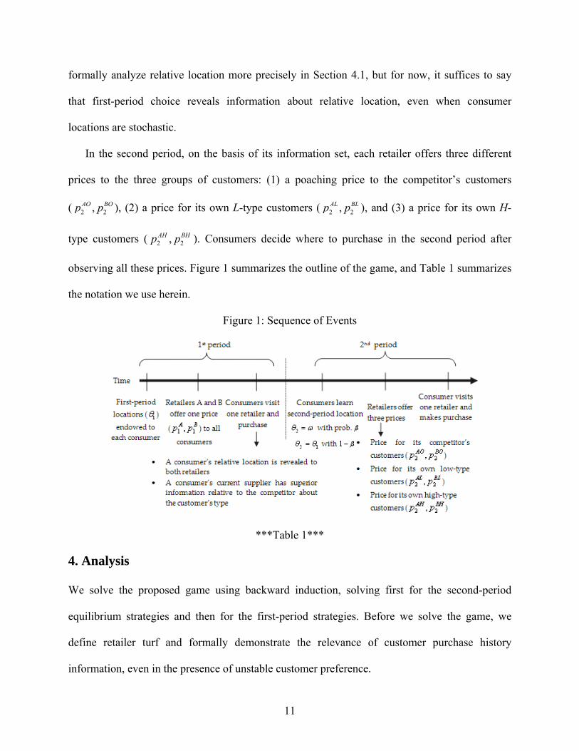
In the second period, on the basis of its information set, each retailer offers three different
prices to the three groups of customers: (1) a poaching price to the competitor’s customers
( 2 2,AO BOp p ), (2) a price for its own L-type customers ( 2 2,AL BLp p ), and (3) a price for its own H-
type customers ( 2 2,AH BHp p ). Consumers decide where to purchase in the second period after
observing all these prices. Figure 1 summarizes the outline of the game, and Table 1 summarizes
the notation we use herein.
Figure 1: Sequence of Events
***Table 1***
4. Analysis
We solve the proposed game using backward induction, solving first for the second-period
equilibrium strategies and then for the first-period strategies. Before we solve the game, we
define retailer turf and formally demonstrate the relevance of customer purchase history
information, even in the presence of unstable customer preference.
12
4.1. Retailer Turf and the Value of Purchase History Information
For any pair of first-period prices (all consumers purchase and both retailers have positive sales),
there is a cut-off 1j
( { , }j L H ), such that all consumers of type j whose 1j
decide to
purchase from retailer A, and the rest purchase from retailer B. Following Fudenberg and Tirole
(2000), we say that consumers to the left of 1j
lie in retailer A’s turf and those on the right lie in
retailer B’s turf to emphasize consumers’ relative locations on the Hotelling line.
For consumers who purchased from retailer A in the first period, retailer A offers the prices
2 2,AH ALp p to H- and L-type customers, respectively, whereas retailer B offers the price 2BOp to
both types at the beginning of the second period. Similarly, among consumers who purchased
from retailer B in the first period, retailer B charges 2 2,BH BLp p , whereas retailer A charges 2 .AOp 10
Given preference correlation in the second period ( 2 1(1 )E , where [0,1]
and ~ [0,1]U ), the conditional probability that consumers will locate in a certain range of the
Hotelling line, given their first-period purchase choice of A or B, is as follows:
1
12 11
1
(1 ) if ,Pr[ ]
(1 ) if ,
x xx x
x x
(1)
1
12 11
1
(1 ) (1 ) if ,Pr[ ] 1
(1 ) (1 ) if .1
x xx x
x x
(2)
Note that Equations (1) and (2) both indicate the general conditional probabilities of the second-
period locations, assuming that a consumer purchases from retailer A or B in the first period.
Therefore, we offer the following lemma:
10 When we analyze the symmetric case, “no poaching” does not arise in equilibrium, but in the asymmetric case, when 1
1 4 , A’s turf is very small and consists only of consumers with a strong preference for A, and retailer A can
charge a monopoly price but not lose any sales to retailer B.
13
Lemma 1 (Value of Purchase History Information): When stochasticity in preference is not
extreme ( 12(1 )z , where z is first-period market share), a consumer who purchases from
retailer j ( { , }j A B ) in period 1 is more likely to stay in the same retailer’s turf rather than
move to the competitor’s turf.
Proof: See Appendix.
This lemma shows that the customer’s first-period purchase is probabilistically informative
of second-period preference, because she or he is more likely to remain in the same turf unless
preference is extremely stochastic. For example, consider the specific case of 11 2 and 1
2 .
A consumer in A’s turf relocates to the same turf with a probability of 34 and relocates to B’s turf
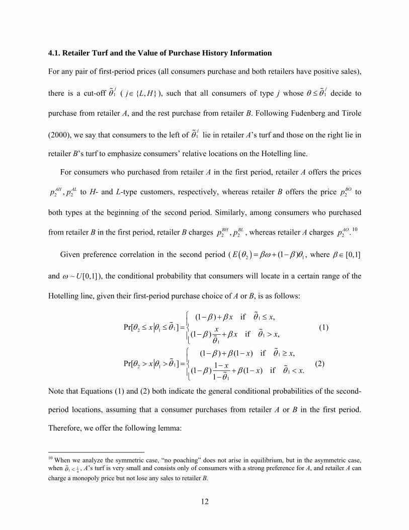
with only a probability of 14 .11 Figure 2 illustrates the redistribution of customer locations in the
second period for four H-type and L-type first-period customers of A. Each letter represents one
H- or L-type consumer. Probabilistically, three H- and L-type consumers remain relatively close
to retailer A, and one of each type changes his or her location toward retailer B in the second
period, as indicated by the arrows in Figure 2.
Note that retailers do not know the exact locations of their own customers in the first period,
but they know their relative location, in that these customers must be somewhere on their turf. In
the second period, retailers still do not know the exact locations of their first-period customers,
but they can assess the average probability of the relative proximity (closer to A or B) of their
first-period customers.
When the turf is symmetric ( 11 2 ), a customer is always more likely to stay on the same
turf for all [0,1) . When 1 (complete independence in preferences), not surprisingly, they
11 Lemma 1 focuses on the horizontal information about the customer’s first-period relative location, as observed from past purchases. Past purchases also reveal vertical information about the customer quantities, which is always valuable, irrespective of the degree of preference stochasticity.
14
are equally likely to appear in either turf in the second period. Thus, past purchases are
informative of future preferences for all [0,1).
Figure 2: Redistribution of Consumer Locations for Consumers in Retailer A’s Turf
4.2. Second Period
A consumer in retailer A’s turf purchases again from retailer A in the second period if and only if
, where { , }j L H and
. Otherwise, the consumer switches to retailer B. We denote the repeat purchase
probability of the high and low types for retailer A as Pr AH and Pr AL , respectively. Thus,
2 21 ( )12 12Pr Pr[ ]
BO AH Hq p pAH and 2 21 ( )
12 12Pr Pr[ ]BO AL Lp pAL
, where 1j
is the
first-period cut-off for type { , }j L H . The repeat purchase probabilities for retailer B similarly
are 2 21 ( )12 12Pr Pr[ ]
BH AO Hq p pBH and PrBL 2 21
12 12Pr[ ]BL AO Lp p
.
The second-period profits of retailers A and B then are
1 1 1 12 2 2 2
1 1 1 12 2 2 2
Pr (1 ) Pr (1 )(1 Pr ) (1 )(1 )(1 Pr ) ,
(1 ) Pr (1 )(1 ) Pr (1 Pr ) (1 ) (1 Pr ) .
H L H LA AH AH AL AL AO BH BL
H L H LB BH BH BL BL BO AH AL
p q p p q
p q p p q
(3)
2 21 ( )22 2 2 2 2 2(1 )
Ajj BO j AjQ p Q pj j Aj j j BOQ v Q p Q v Q p
1,L HQ Q q
15
Each retailer’s second-period demand consists of three parts. For example, retailer A enjoys
demand from (1) its own previous H-type customers ( 1H
), who continue to be in the retailer’s
turf in the second period (with probability Pr AH ) and pay a price 2AHp ; (2) its own previous L-
type customers ( 1L
), who continue to be in the retailer’s turf in the second period (with
probability Pr AL ) and pay a price 2ALp ; and (3) a mix of the competitor’s previous high- and low-
type customers ( 1 1(1 ) (1 )H L
) who have shifted to the retailer’s turf (with probability
1 PrBj , where { , }j L H ) and pay a price 2AOp .
Using Equations (1) and (2), we can obtain the second-period prices by solving the retailers’
first-order conditions. We only look for the pure strategy equilibrium in a symmetric game. In
the first-period analysis, we show that the symmetric outcome, in which both firms charge the
same price in the first period, is indeed the equilibrium solution.
Proposition 1: Suppose there exists a non-zero portion of H-type customers in the market
( 0 1 ).
(a) Reward Competitor’s Customers: When preference stochasticity is low
(
2
2
2 3 1 2
3 1 4( , )
q q
q qq
), there exists a symmetric pure strategy equilibrium in second-
period prices, such that retailers charge 2
2 1 ( 1)12 2 2 6 2 1 ( 1)
,qAH BHq q
p p
2 2
AL BLp p
2
2 1 ( 1)12 6 2 1 ( 1)
,q
q
and
2
2 1 ( 1)2 2 3 2 1 ( 1)
.qAO BO
qp p
Prices follow an ordinal relationship,
2 2 2iO iH iLp p p , where { , }i A B ; that is, the competitor’s customers receive the lowest price.
(b) Reward Own Best Customers: When preference stochasticity is sufficiently high
22 2 2
2
2 ( 6)(1 ) 2 ( 6)(1 ) 12(1 ) 4 ( 3)(1 )
4 ( 3)(1 )( ( , ) )
q q q q q q
q qq
and consumer heterogeneity in
16
purchase quantity is sufficiently high (2 9(1 )1 1 46 47
8 5 3max{ , }q
), there exists a symmetric
pure strategy equilibrium in second-period prices, such that retailers charge
2
2 1 ( 1)22 2 2 6 2 1
,qAH BHq q
p p
2
2 1 ( 1)12 2 2 6 2 1
,qAL BL
qp p
and 2 2
AO BOp p
2
2 1 ( 1)
3 2 1.q
q
Prices follow an ordinal relationship, 2 2 2
iH iO iLp p p , where { , }i A B ; that is,
the retailer’s own high-type customers receive the lowest price. 12
Proof. See Appendix.
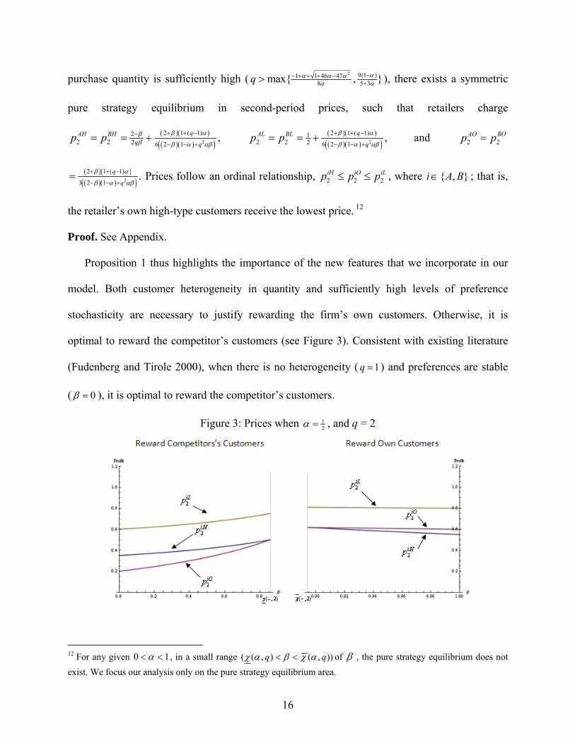
Proposition 1 thus highlights the importance of the new features that we incorporate in our
model. Both customer heterogeneity in quantity and sufficiently high levels of preference
stochasticity are necessary to justify rewarding the firm’s own customers. Otherwise, it is
optimal to reward the competitor’s customers (see Figure 3). Consistent with existing literature
(Fudenberg and Tirole 2000), when there is no heterogeneity ( 1q ) and preferences are stable
( 0 ), it is optimal to reward the competitor’s customers.
Figure 3: Prices when 12 , and q = 2
12 For any given 0 1 , in a small range ( ( , ) ( , ))q q of , the pure strategy equilibrium does not
exist. We focus our analysis only on the pure strategy equilibrium area.
17
The intuition for why both customer heterogeneity and sufficient preference stochasticity are
needed to reward the firm’s own customers is as follows: As Lemma 1 shows, in a symmetric
market, customers are more likely to stay with the current retailer than they are to switch to a
rival for all [0,1) . If customers are all equal in value (i.e., no customer heterogeneity in
quantity), retailers take advantage of customers’ revealed preferences from the previous purchase
and charge a higher price to their own customers, and expend more effort to acquire the
competitor’s customers through low prices. Although retailers understand that some existing
customers switch in the second period (though they cannot identify exactly who; they only know
the aggregate probability of customers changing turfs), they do not find it optimal to offer a
lower price to their current customers, because the potential loss from existing customers can be
more than compensated for by the newly acquired competitor’s customers since both own and
competitor’s customers are all equal in value.
However, if customers are heterogeneous, retailers must assess whether selective retention
(rewarding own best customers) is profitable. The value of the firm’s own high-type customers is
greater than the expected average value of the competitor’s customers. Furthermore, as
preference stochasticity increases, the monopoly power that the retailer enjoys from horizontal
preference weakens. Beyond a certain threshold of preference stochasticity, the marginal gain in
profit from retaining high-type customers through lowered prices becomes greater than the
marginal benefit of poaching a mix of high- and low-type competitor’s customers. Therefore,
both heterogeneity in quantities and high levels of preference stochasticity are necessary to make
rewarding the firm’s own high-type customers an effective strategy.
Finally, it is never optimal to offer a better value to own low-type customers, whose value is
less than the expected average value of the competitor’s customers. They always receive the
18
highest price offer. This result echoes practitioners’ assertion that the firm must reward its own
best customers (not all of its customers!)13
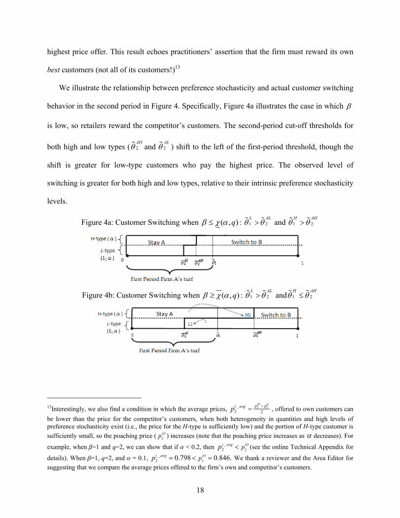
We illustrate the relationship between preference stochasticity and actual customer switching
behavior in the second period in Figure 4. Specifically, Figure 4a illustrates the case in which
is low, so retailers reward the competitor’s customers. The second-period cut-off thresholds for
both high and low types ( 2AH
and 2AL
) shift to the left of the first-period threshold, though the
shift is greater for low-type customers who pay the highest price. The observed level of
switching is greater for both high and low types, relative to their intrinsic preference stochasticity
levels.
Figure 4a: Customer Switching when ( , )q : 1 2L AL
and 1 2H AH
Figure 4b: Customer Switching when ( , )q :
1 2L AL
and 1 2H AH
13Interestingly, we also find a condition in which the average prices, 2 2_
2 2
iH iLp pi avgp , offered to own customers can
be lower than the price for the competitor’s customers, when both heterogeneity in quantities and high levels of preference stochasticity exist (i.e., the price for the H-type is sufficiently low) and the portion of H-type customer is
sufficiently small, so the poaching price ( 2
iOp ) increases (note that the poaching price increases as decreases). For
example, when b=1 and q=2, we can show that if a < 0.2, then 2
_2
iOi avg pp (see the online Technical Appendix for
details). When b=1, q=2, and a = 0.1, 2
_2 0.798 0.846.iOi avg pp We thank a reviewer and the Area Editor for
suggesting that we compare the average prices offered to the firm’s own and competitor’s customers.
19
In Figure 4b, we present the case when is high, so retailers reward their own best
customers. An H-type customer (H1) who bought from retailer A in the first period but gets a
shock in the second period that moves him closer to retailer B, still remains with retailer A. An L-
type customer (L1) who bought from retailer A and receives a shock that makes her even closer to
retailer A instead may switch in the second period. In effect, the observed level of switching
among H-types is lower relative to their preference stochasticity level, because they still
repurchase from the same retailer even though they are much closer to the alternative. In contrast,
the observed level of switching among L-type customers is greater than their preference
stochasticity level. Even if the level of preference stochasticity is identical for the two types (i.e.,
no exogenous relationship between quantity and loyalty), firms’ BBP practice creates an
endogenous tendency for the most valuable (H-type) customers to stay more loyal than do L-type
customers.14
4.3. First Period
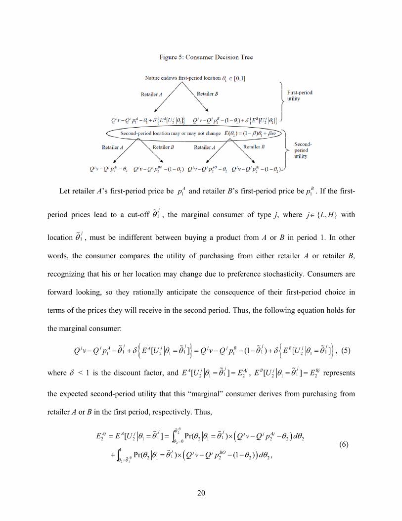
In the first period, the forward-looking consumer solves a dynamic program that takes into
account the probabilities of second-period location and the prices offered by both retailers, as we
show in Figure 5. Because these prices are the outcome of a dynamic strategic game played by
the retailers, solving for the equilibrium retailer and consumer strategies requires embedding the
consumer’s dynamic programming problem within a dynamic strategic game that involves one
price for each retailer in the first period and three prices (own high and low types, and
competitor’s customers) for each retailer in the second period.
14 We thank the Editor for suggesting an analysis of the interplay between quantity and customer loyalty. To this end, we consider the possibility of different preference stochasticity levels across two segments, say b for L-type and kb for H-type. Our main result—pertaining to rewarding the firm’s own customers by offering them a lower price beyond a certain threshold level of b—remains robust as long as kb is higher than a threshold level, that is, if the preference stochasticity of the high types is not much lower than that of the low types. However, if kb for H-type customers is extremely low (i.e., little preference stochasticity), the firm has no incentive to reward its own high-type customers, who are very likely to stay with the firm. The Technical Appendix on the Web provides details.
20
Let retailer A’s first-period price be 1Ap and retailer B’s first-period price be 1
Bp . If the first-
period prices lead to a cut-off 1j
, the marginal consumer of type j, where { , }j L H with
location 1j
, must be indifferent between buying a product from A or B in period 1. In other
words, the consumer compares the utility of purchasing from either retailer A or retailer B,
recognizing that his or her location may change due to preference stochasticity. Consumers are
forward looking, so they rationally anticipate the consequence of their first-period choice in
terms of the prices they will receive in the second period. Thus, the following equation holds for
the marginal consumer:
1 1 1 11 2 1 1 2 1[ ] (1 ) [ ]j j j jj j A A j j j B B jQ v Q p E U Q v Q p E U , (5)
where < 1 is the discount factor, and 12 1 2[ ]jA j AjE U E ,
12 1 2[ ]jB j BjE U E represents
the expected second-period utility that this “marginal” consumer derives from purchasing from
retailer A or B in the first period, respectively. Thus,
2
2
2 2
1 12 2 1 2 1 2 2 20
1
12 1 2 2 2
[ ] Pr( )
Pr( ) (1 ) ,
Aj
Aj
j jAj A j j j Aj
j j j BO
E E U Q v Q p d
Q v Q p d
(6)
21
2
2
2 2
1 12 2 1 2 1 2 2 20
1
12 1 2 2 2
[ ] Pr( )
Pr( ) (1 ) ,
Bj
Bj
j jBj B j j j AO
j j j Bj
E E U Q v Q p d
Q v Q p d
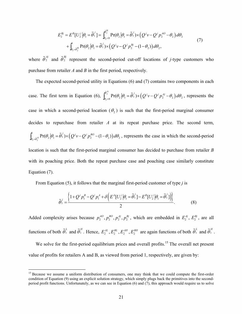
(7)
where 2Aj
and 2Bj
represent the second-period cut-off locations of j-type customers who
purchase from retailer A and B in the first period, respectively.
The expected second-period utility in Equations (6) and (7) contains two components in each
case. The first term in Equation (6),
2
2
12 1 2 2 20Pr( )
Ajj j j AjQ v Q p d
, represents the
case in which a second-period location ( 2 ) is such that the first-period marginal consumer
decides to repurchase from retailer A at its repeat purchase price. The second term,
2 2
1
12 1 2 2 2Pr( ) (1 )Aj
j j j BOQ v Q p d
, represents the case in which the second-period
location is such that the first-period marginal consumer has decided to purchase from retailer B
with its poaching price. Both the repeat purchase case and poaching case similarly constitute
Equation (7).
From Equation (5), it follows that the marginal first-period customer of type j is
1 11 1 2 1 2 1
1
1 [ ] [ ].
2
j jj B j A A j B j
jQ p Q p E U E U
(8)
Added complexity arises because 2 2 2 2, , ,AO BO Aj Bjp p p p , which are embedded in 2 ,AjE 2BjE , are all
functions of both 1 1 and .L H
Hence, 2ALE , 2
BLE , 2AHE , 2
BHE are again functions of both 1 1and L H
.
We solve for the first-period equilibrium prices and overall profits.15 The overall net present
value of profits for retailers A and B, as viewed from period 1, respectively, are given by:
15 Because we assume a uniform distribution of consumers, one may think that we could compute the first-order condition of Equation (9) using an explicit solution strategy, which simply plugs back the primitives into the second-period profit functions. Unfortunately, as we can see in Equation (6) and (7), this approach would require us to solve

22
1 11 2
1 11 2
( ) ,
( ) (1 ) (1 ) ,
H LA A A
H LB B B
p q
p q
(9)
where 2 2,A B are as defined in Equation (3).
Taking first-order conditions with respect to prices, we find a symmetric pure strategy
equilibrium in which both retailers charge the same prices (by using the envelope theorem and
indirect method to solve for the first-order conditions that we develop in Lemma 2 in Appendix,
we can arrive at the closed form solutions; see the Appendix for details):
1 1
1 1
1 1
1 1
(1 ) 2
1 12 (1 )
H LH H
A Ap p
H L
A Ap p
qA B
q
p p
, (10)
2 2 2 2 2 2 2 2
2 2 21 1 1 1 1
,L
AA BO AB BL AB BH AA AB
BO L BL L BH L L L
dp dp dp
p p pd d d
2 2 2 2 2 2 2 2
2 2 21 1 1 1 1
.H
AA BO AB BL AB BH AA AB
BO H BL H BH H H H
dp dp dp
p p pd d d
Therefore, the equilibrium profits are
1 1
1 1
1 1
1 1
(1 ) 2(1 )
1 21 2 222 (1 )
( ) (1 ) .
H LH H
A Ap p
H L
A Ap p
qH L qA B A A A
q
p q
(11)
We now compare these profits obtained by BBP with a model that does not use customer
purchase information. The comparison should help us understand the benefits, if any, of BBP.
The model that does not use customer purchase information reduces to a static pricing model.
In each period, the two retailers maximize their current profits. In this static pricing scenario,
both retailers would charge the static price ( 1sp ), which maximizes the static profit functions in
each period, such that
the integral with the boundary and the probability itself involving the primitives of 1
j
, which is again the implicit
function of itself and 1
Ap . It is therefore infeasible to employ this explicit solution strategy. We follow and extend
the general approach, first employed by Fudenberg and Tirole (2000). Furthermore, we develop an indirect method to solve this challenge, which we show in Lemma 2 of the Appendix.
23
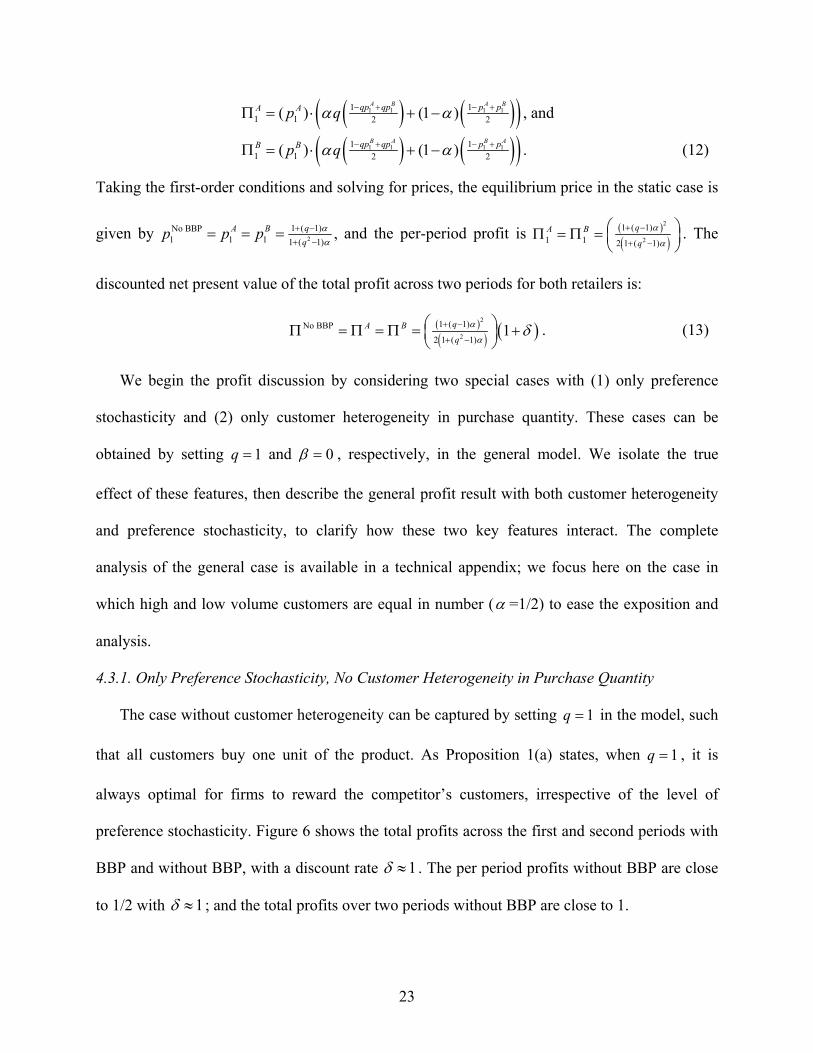
1 1 1 11 11 1 2 2( ) (1 )
A B A Bqp qp p pA Ap q , and
1 1 1 11 11 1 2 2( ) (1 )
B A B Aqp qp p pB Bp q . (12)
Taking the first-order conditions and solving for prices, the equilibrium price in the static case is
given by 2
1 ( 1)No BBP1 1 1 1 ( 1)
,qA B
qp p p
and the per-period profit is
2
2
1 ( 1)1 1 2 1 ( 1)
qA B
q
. The
discounted net present value of the total profit across two periods for both retailers is:
2
2
1 ( 1)No BBP
2 1 ( 1)1qA B
q
. (13)
We begin the profit discussion by considering two special cases with (1) only preference
stochasticity and (2) only customer heterogeneity in purchase quantity. These cases can be
obtained by setting 1q and 0 , respectively, in the general model. We isolate the true
effect of these features, then describe the general profit result with both customer heterogeneity
and preference stochasticity, to clarify how these two key features interact. The complete
analysis of the general case is available in a technical appendix; we focus here on the case in
which high and low volume customers are equal in number ( =1/2) to ease the exposition and
analysis.
4.3.1. Only Preference Stochasticity, No Customer Heterogeneity in Purchase Quantity
The case without customer heterogeneity can be captured by setting 1q in the model, such
that all customers buy one unit of the product. As Proposition 1(a) states, when 1q , it is
always optimal for firms to reward the competitor’s customers, irrespective of the level of
preference stochasticity. Figure 6 shows the total profits across the first and second periods with
BBP and without BBP, with a discount rate 1 . The per period profits without BBP are close
to 1/2 with 1 ; and the total profits over two periods without BBP are close to 1.
24
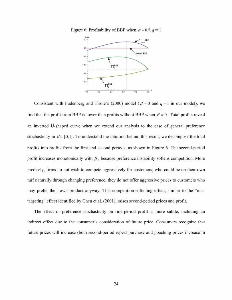
Figure 6: Profitability of BBP when 0.5, q = 1
Consistent with Fudenberg and Tirole’s (2000) model ( 0 and 1q in our model), we
find that the profit from BBP is lower than profits without BBP when 0 . Total profits reveal
an inverted U-shaped curve when we extend our analysis to the case of general preference
stochasticity in [0,1] . To understand the intuition behind this result, we decompose the total
profits into profits from the first and second periods, as shown in Figure 6. The second-period
profit increases monotonically with , because preference instability softens competition. More
precisely, firms do not wish to compete aggressively for customers, who could be on their own
turf naturally through changing preference; they do not offer aggressive prices to customers who
may prefer their own product anyway. This competition-softening effect, similar to the “mis-
targeting” effect identified by Chen et al. (2001), raises second-period prices and profit.
The effect of preference stochasticity on first-period profit is more subtle, including an
indirect effect due to the consumer’s consideration of future price. Consumers recognize that
future prices will increase (both second-period repeat purchase and poaching prices increase in
25
), so their choices become less sensitive to changes in the first-period price. The lower price
sensitivity shifts first-period price upward as increases.16
However, a countervailing direct effect exerts downward pressure on first-period prices. As
increases, the link between customers’ choices in the first and second periods weakens,
because consumer preferences become less correlated, and price elasticity in the first period is
less affected by what happens in the second period. The direct effect interacts with the indirect
effect and effectively weakens the upward pressure of the indirect effect. At the extreme, when
1 , demand in the two periods becomes independent, and price elasticity increases to short-
run elasticity without BBP; in turn, profits with and without BBP become identical.
In summary, the net effect on first-period price (upward pressure from indirect effect and
downward pressure from direct effect) leads to an inverted U-shaped curve for first-period
profits (and total profits). Therefore, the total equilibrium profit is maximized at 0.6435 ,
increasing for 0,0.6435 and decreasing for 0.6435,1 .
4.3.2. No Stochastic Preference , Only Customer Heterogeneity in Purchase Quantity
When there is no changing preference ( 0 ), we know from Proposition 1 that retailers
offer the lowest price to their competitor’s customers; therefore, 2 2 2iO iH iLp p p . However, the
more surprising result indicates that when heterogeneity in purchase quantities is sufficiently
high, the total profit with BBP is greater than profits without BBP.
16 More precisely, the indirect effect of consumer’s future consideration affects the first-period price in two ways: (1) Second-period high repeat purchase prices decrease price elasticity in the first period, because customers know they will be ripped off by the same firm in the second period (ratchet effect), and (2) second-period low poaching price increases price elasticity in the first period, causing a downward pressure on prices. As β increases, both poaching and repeat purchase prices increase, and the correct expectation of high prices makes consumers less price sensitive in the first period (higher repeat purchase price further decreases price elasticity; higher poaching price weakens upward pressure on price elasticity). The indirect effect through a consumer’s dynamic consideration makes first-period demand less elastic, causing firms to increase prices and profits in the first period as β increases.
26
Proposition 2. Suppose there is no preference stochasticity ( 0 ). If heterogeneity in purchase
quantities is sufficiently high (q > 5), both retailers increase their profits under BBP.
Proof. See Appendix.
Thus, BBP can increase both competing firms’ profits even when consumer preferences are
stable if there is sufficient heterogeneity in quantities. This result does not occur simply because
of heterogeneity in quantities and the ability to distinguish between high- and low-type
customers. The asymmetric information about customer types is critical.
The intuition for this result is as follows: With asymmetric information, the poacher faces an
adverse selection (lemon) problem when attracting the competitor’s customers. Because the high
types get lower prices from their current retailer, firms recognize that poaching
disproportionately attracts L-type relative to H-type customers. Therefore, firms become less
aggressive in attracting the competitor’s customers as customer heterogeneity becomes
significant (i.e., degree of adverse selection becomes greater). In other words, asymmetric
customer information softens competition, so the benefit of price discrimination dominates the
cost of increased competition typically associated with BBP when customer heterogeneity
becomes significant.
4.3.3. Both Stochastic Preference and Customer Heterogeneity in Purchase Quantity
We next consider the full model by relaxing both the q=1 and 0 assumptions.
Specifically, we consider the q=2 case to allow for customer heterogeneity, which helps build the
intuition for the customer heterogeneity case with the least complexity.
In Figure 7, we show the total profits with and without BBP when 0.5, and 2q . As
anticipated from Proposition 1, there are two regimes based on the pricing strategy in period 2:
the “reward competitor’s customers” regime and the “reward own best customers” regime. As a
27
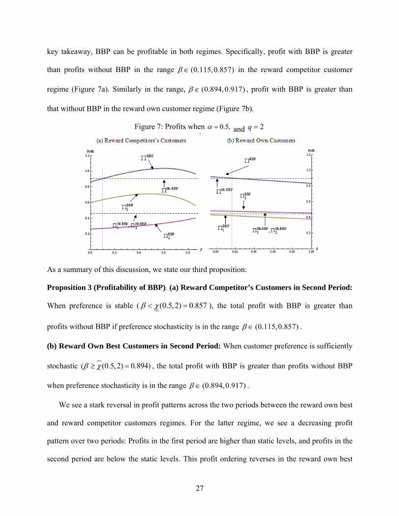
key takeaway, BBP can be profitable in both regimes. Specifically, profit with BBP is greater
than profits without BBP in the range (0.115,0.857) in the reward competitor customer
regime (Figure 7a). Similarly in the range, (0.894,0.917) , profit with BBP is greater than
that without BBP in the reward own customer regime (Figure 7b).
Figure 7: Profits when 0.5, and 2q
As a summary of this discussion, we state our third proposition:
Proposition 3 (Profitability of BBP). (a) Reward Competitor’s Customers in Second Period:
When preference is stable ( (0.5,2) 0.857 ), the total profit with BBP is greater than
profits without BBP if preference stochasticity is in the range (0.115,0.857) .
(b) Reward Own Best Customers in Second Period: When customer preference is sufficiently
stochastic ( (0.5,2) 0.894) , the total profit with BBP is greater than profits without BBP
when preference stochasticity is in the range (0.894,0.917) .
We see a stark reversal in profit patterns across the two periods between the reward own best
and reward competitor customers regimes. For the latter regime, we see a decreasing profit
pattern over two periods: Profits in the first period are higher than static levels, and profits in the
second period are below the static levels. This profit ordering reverses in the reward own best
28
customers regime, so that we see an increasing profit pattern over time; that is, the first-period
profits are below the static levels, whereas second period profits are above.
The intuition for profits under the reward competitors' customer regime follows directly from
the previous discussion regarding the direct and indirect effects of preference stochasticity alone
and the discussion of information asymmetry with only heterogeneity. On the other hand, the
intuition for the increasing price and profit pattern over time under the reward own best
customers regime follows from the lock-in intuition, similar to switching cost models
(Klemperer 1995, Farrell and Klemperer 2007). Firms compete to attract more customers in the
first period to gain an information advantage about customer types. By using this information
advantage, firms effectively can lock in their most valuable (and profitable) H-type customers by
rewarding them in the second period.17 This lock-in intuition explains the profit pattern over
time—that is, lower first-period profit and higher second-period profit. Moreover, we find that
firms can be better off with BBP under this regime.
However, as preference stochasticity gets closer to 1, the benefit of lock-in weakens due to
the imperfect lock-in that arises from preference stochasticity, which in turn lowers the second-
period profits. At high levels of preference stochasticity, overall profits can be lower with BBP
when 0.5, and q = 2. In general, the total profit can be higher with BBP even when
preference stochasticity is very high, because of the same adverse selection intuition in the pure
heterogeneity case. For example, when a = 0.5, BBP is always profitable if q ≥ 5. The threshold
level of preference stochasticity at which the total profit with BBP is greater than that without
BBP is 0.917 when 0.5, and q = 2.
17 In our model, the high types are indeed the most valuable customers for firms, because the optimal prices are such
that per period profits will be higher for the high type (that is, 1
2 2 22
AH AO ALqq p p p for all and 2q ). In
other words, the cost to retain high types does not exceed the benefit of retaining them. Furthermore, it is easy to see
that second-period prices are all higher than the first-period price, 2 1
AH Ap p .
29
This threshold is in fact a function of a and q. When the value of information asymmetry is
greater (larger q), the threshold rises, and rewarding own best customers is a profitable strategy
for a wider range of preference stochasticity. For example, when q = 16, which is the case
suggested by the 80/20 rule when a = 0.5,18 the range in which BBP is profitable under the
reward own best customers regime becomes much larger, b œ (0.731, 0.961).
5. Conclusion
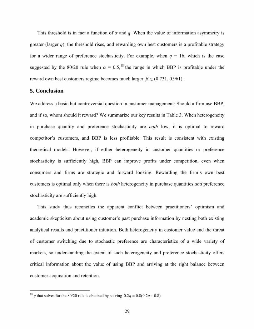
We address a basic but controversial question in customer management: Should a firm use BBP,
and if so, whom should it reward? We summarize our key results in Table 3. When heterogeneity
in purchase quantity and preference stochasticity are both low, it is optimal to reward
competitor’s customers, and BBP is less profitable. This result is consistent with existing
theoretical models. However, if either heterogeneity in customer quantities or preference
stochasticity is sufficiently high, BBP can improve profits under competition, even when
consumers and firms are strategic and forward looking. Rewarding the firm’s own best
customers is optimal only when there is both heterogeneity in purchase quantities and preference
stochasticity are sufficiently high.
This study thus reconciles the apparent conflict between practitioners’ optimism and
academic skepticism about using customer’s past purchase information by nesting both existing
analytical results and practitioner intuition. Both heterogeneity in customer value and the threat
of customer switching due to stochastic preference are characteristics of a wide variety of
markets, so understanding the extent of such heterogeneity and preference stochasticity offers
critical information about the value of using BBP and arriving at the right balance between
customer acquisition and retention.
18 q that solves for the 80/20 rule is obtained by solving 0.2 0.8(0.2 0.8).q q
30
Table 3: Summary of Results
Certain limitations of our model suggest interesting directions for further research. First, we
do not allow consumers to split their purchases across different firms or even across periods;19
thus, it is harder for firms to infer the customer’s true potential and share of customer wallet. In
our current model, the first-period purchases help firms unambiguously identify H- and L-type
consumers. When consumers can split their purchases, the inference about consumer type would
be only probabilistic, even if firms possess share-of-wallet information. Thus, share-of-wallet
information weakens the extent of information asymmetry in the model (see Du and Kamakura
2008 as an example for how a firm may infer share of wallet).
Second, third parties also sell estimates of customer spending potential, based on the
observed characteristics of the household (e.g., zip code, demographics), but this information is
far from perfect. Therefore, even with third-party information, the observed purchase history still
provides the information asymmetry critical to the profitability of BBP. We therefore believe our
findings are robust even with the introduction of noisy potential information, though it might
weaken the information asymmetry. A systematic analysis of how share of wallet and potential 19 Consumers may strategically time their purchases. This could be related to sales force literature where in response to quotas and bonuses, sales people sometimes shift their effort and book sales towards the end of the year to qualify for a bonus (Steenburgh 2008). We thank an anonymous reviewer for raising this issue.

31
estimates may affect information asymmetry, and their resulting effect on BBP, would offer an
important next step from both the empirical and theoretical perspectives.20
Third, given our focus on BBP, we have abstracted away from modeling second-degree price
discrimination. Our model is a reasonable abstraction of many real-world markets (e.g., airlines,
department stores, grocery stores), in which firms only use BBP with past customer purchase
history data but do not offer a menu of prices. This could be because consumers differ not in the
quantity they use at any one time but in the frequency of their use. Firms need to aggregate the
flow of multiple purchases across a certain time period into a “past quantity” stock. In this
scenario, menu pricing is not feasible, and BBP is appropriate. Nevertheless, further research
needs to consider how robust our results are if competitors could offer a menu of poaching prices.
The second-degree price discrimination problem in a competitive setting with customer behavior
information is a technical challenge that has not yet been solved generally and awaits further
research (Stole 2007). We therefore leave the issue of combining BBP and second-degree price
discrimination as an important, but challenging, area of further research.
Fourth, our theoretical model provides empirically testable hypotheses for further research.
We find that BBP is most likely effective when there is sufficient heterogeneity in customer
quantities and preference stochasticity. Empirical research across categories which vary along
these dimensions can help ascertain whether these predictions are valid. We therefore hope our
model serves as an impetus for further theoretical and empirical research into BBP.
20 A potential formulation that accommodates the notion of share of wallet and customer potential might be q = Potential S(q), where S(q) the share of wallet of the customer, is a function of the relative preference between firms (i.e., based on location q).

32
Appendix
Proof of Lemma 1 (Value of information).
We first address retailer A. Let z be the first-period market share. Then,
2 1 2 1Pr[ ] Pr[ ] (1 ) (1 ).z z z z z z In turn, 2 1Pr[ ]z z
2 1Pr[ ]z z 12(1 )0 .z Therefore, it always holds when 1
2(1 )z . In particular, when
12z , the inequality always holds for (0,1] . Next, let 1z z be retailer B’s first-period
market share and substitute it into Equation (2). We get the exactly same result. Q.E.D.
Proof of Proposition 1 (Reward own customers or competitor’s customers).
(a) We start with
2
2
2 3 1 2
3 1 4( , )
q q
q qq
, where ( , ) ( , )q q for (0,1) , which
ensures that 1 2L AL
and 1 2H AH
, in equilibrium. Again, using Equations (1) and (2), we
know that 2 2
1
1 ( )12Pr ,
BO AH
H
q p pAH
2 2
1
112Pr ,
Bo AL
L
p pAL
PrBH
2 2
1
1 ( )121
( )BH Ao
L
q p p
, and 2 2
1
1121
Pr ( )BL AO
L
p pBL
. Similar to the proof of Proposition 1, we
solve the first-order conditions. When 11 2
j , second-period prices are
2
2 1 ( 1)12 2 2 6 2 1 ( 1)
,qAH BHq q
p p
2 2
AL BLp p 2
2 1 ( 1)12 6 2 1 ( 1)
q
q
, and
2
2 1 ( 1)2 2 3 2 1 ( 1)
,qAO BO
qp p
which confirms that 1 2L AL
and 1 2H AH
when
2
2
2 3 1 2
3 1 4( )
q q
q qq
. We only need to
show that 2 2 2iO iH iLp p p . First, we notice that
2
2
2 3 1 2
3 1 4( )
q q
q qq
is an increasing function in
[0,1] for any 1q . Second, we have
2
22
2 5 1 62 1 ( 1) 12 2 2 7 1 66 2 1 ( 1)
q qqiO iHq q qq
p p
,

33
and
2
2
2 5 1 6
7 1 61
q q
q q
for any 1q and [0,1] . Hence, the inequality always satisfies for all
1q . In addition, it is obvious that 1 12 2 2 2iH iL
qp p for all 1q . ■
(b) Next, we look at the case ( )q , which ensures that in equilibrium, the market is
1 2L AL
and 1 2H AH
, where 22 2 2
2
2 ( 6)(1 ) 2 ( 6)(1 ) 12(1 ) 4 ( 3)(1 )
4 ( 3)(1 )( )
q q q q q q
q qq
. Again,
from Equations (1) and (2), we know that 2 21 ( )2Pr (1 ) ,
BO AHq p pAH
2 2
1
112Pr ,
Bo AL
L
p pAL
2 21 ( )
2Pr (1 ) ( ),BH Aoq p pBH and PrBL 2 2
1
1121
( )BL AO
L
p p
.
Plugging these into Equation (3), we obtain the second-period prices by solving the retailers’
first-order conditions. Specifically, when 11 2
j , the second-period prices are
2
2 1 ( 1)22 2 2 6 2 1
,qAH BHq q
p p
2
2 1 ( 1)12 2 2 6 2 1
,qAL BL
qp p
and
2
2 1 ( 1)2 2 3 2 1
.qAO BO
qp p
We confirm that
1 2L AL
and 1 2H AH
when 1q and ( ).q
First, we verify that 2
(2 )(1 ) 2 212 6( 1)(2 )
0 2(3 2) (3 4)qiL iO iL iO
qp p p p q q q q
.
Note that 2 2(3 4) (3 4)q q q q for [0,1] . Hence, the result that iL iOp p for all
[0,1] and 1q derives directly from 2 22(3 2) (3 4) 3 ( 1) 0q q q q q q . Second,
we show that iH iOp p . Notice that 2
(2 )(1 )2
6( 1)(2 )( ).qiH iO
q qp p q
We only need to
show that there exists [0,1] , such that
22 2 2
2
2 ( 6)(1 ) 2 ( 6)(1 ) 12(1 ) 4 ( 3)(1 )
4 ( 3)(1 )( , )
q q q q q q
q qq
.
Lemma 1: For all (0,1) , there always exists 2 9(1 )1 1 46 47
8 5 3max{ , }q
, such that
( , ) 1q .
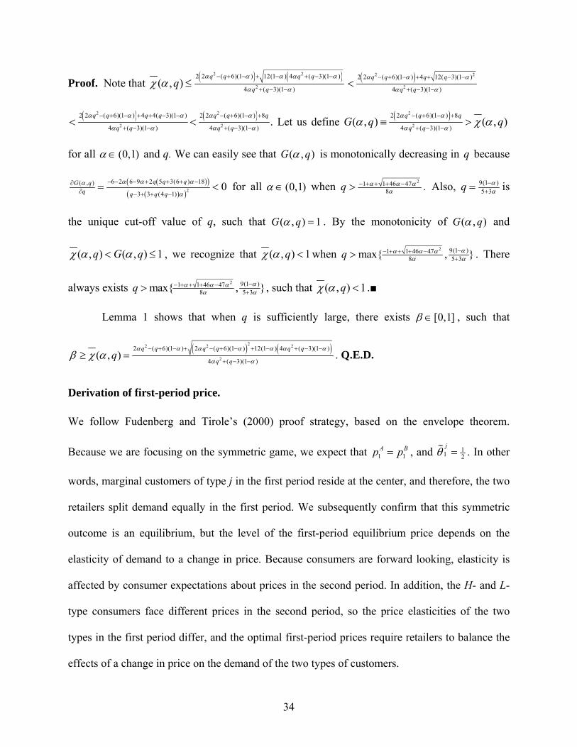
34
Proof. Note that 2 2
2
2 2 ( 6)(1 ) 12(1 ) 4 ( 3)(1 )
4 ( 3)(1 )( , )
q q q q
q qq
2 2
2
2 2 ( 6)(1 ) 4 12( 3)(1 )
4 ( 3)(1 )
q q q q
q q
2 2
2 2
2 2 ( 6)(1 ) 4 4( 3)(1 ) 2 2 ( 6)(1 ) 8
4 ( 3)(1 ) 4 ( 3)(1 ).
q q q q q q q
q q q q
Let us define
2
2
2 2 ( 6)(1 ) 8
4 ( 3)(1 )( , ) ( , )
q q q
q qG q q
for all (0,1) and q. We can easily see that ( , )G q is monotonically decreasing in q because
2
6 2 6 9 2 5 3(6 ) 18( , )
3 3 (4 1)0
q q qG qq q q q
for all (0,1) when 21 1 46 47
8q
. Also, 9(1 )5 3q
is
the unique cut-off value of q, such that ( , ) 1G q . By the monotonicity of ( , )G q and
( , ) ( , ) 1q G q , we recognize that ( , ) 1q when 2 9(1 )1 1 46 47
8 5 3max{ , }q
. There
always exists 2 9(1 )1 1 46 47
8 5 3max{ , }q
, such that ( , ) 1q .■
Lemma 1 shows that when q is sufficiently large, there exists [0,1] , such that
22 2 2
2
2 ( 6)(1 ) 2 ( 6)(1 ) 12(1 ) 4 ( 3)(1 )
4 ( 3)(1 )( , )
q q q q q q
q qq
. Q.E.D.
Derivation of first-period price.
We follow Fudenberg and Tirole’s (2000) proof strategy, based on the envelope theorem.
Because we are focusing on the symmetric game, we expect that 1 1A Bp p , and 1
1 2
j . In other
words, marginal customers of type j in the first period reside at the center, and therefore, the two
retailers split demand equally in the first period. We subsequently confirm that this symmetric
outcome is an equilibrium, but the level of the first-period equilibrium price depends on the
elasticity of demand to a change in price. Because consumers are forward looking, elasticity is
affected by consumer expectations about prices in the second period. In addition, the H- and L-
type consumers face different prices in the second period, so the price elasticities of the two
types in the first period differ, and the optimal first-period prices require retailers to balance the
effects of a change in price on the demand of the two types of customers.

35
Applying the implicit function theorem, we arrive at the following lemma:
Lemma 2. The first-period price sensitivities for L- and H-type consumers are
1 1
1 1
and L HH L L H
H H L LA L H L H A L H L H
L H H L L H H L
F q F q F Fd d
dp F F F F dp F F F F
,
where
1 1
2 ,AL BL
L L
L E ELF
1 1
,AH BH
L L
H E ELF
1 1
,AL BL
H H
L E EHF
1 1
2 .AH BH
H H
H E EHF
Proof: We define the implicit functions from Equation (8) as follows:
1 1 1 1 1 1 11 1 1( , , ) 2 1 ( , ) ( , ) 0,L H L L H L HL A B A AL BLF p p p E E and
1 1 1 1 1 1 11 1 1( , , ) 2 1 ( , ) ( , ) 0.L H H L H L HH A B A AH BHF p qp qp E E
We differentiate both equations and rearrange them as follows:
1
1 111
1
1
,
HL L
A H AL
A L
L
F F dp dpd
dp F
and
1
1 111
1
1
.
LH H
A L AH
A H
H
F F dp dpd
dp F
Solving these two equations simultaneously, we obtain the following results:
1 1
1 1and ,
L HF FL H H LH Lp p p pH L L H L H H LH LL HF FH p H p L p L pH L
A H L L H A L H L HL H L HF F F FL HH L H L L H H LH L H LL HH LF FH L
F F F FF F F F F F F Fd d
dp F F F F dp F F F FF F
Using 1 1
1, ,L H
A A
F FL Hp pp p
F F q
we recognize that
1 1 1
2 ,L AL BL
L L L
FL E ELF
1
H
L
FHLF
1 1
,AH BH
L LE E
and
1 1 1
2 .H AH BH
H H H
FH E EHF
Q.E.D.
It is convenient to rewrite Equation (11) for firm A’s overall profits using the functions
2 2,AA AB to represent its second-period profit from its own previous customers and from
retailer B’s previous customers, respectively:
1 1 1 11 2 2 1 1 2 1 1 1 1 1 1
1 12 2 1 1 2 1 1 1 1 1 1
(1 ) ( , ), ( , ), ( , ), ( , )
( , ), ( , ), ( , ), ( , )
H L L HA A AA Ai A B Bi A B A B A B
L HAB Ai A B Bi A B A B A B
p q p p p p p p p p p p
p p p p p p p p p p
(A-1)

36
where 1 1 1 1 1 12 2 2 2 2 2 2 2 2, , , ( ) Pr , , ( )(1 ) Pr , , ,L H H H L LAA Ai Bi AH AH AH BO AL AL AL BOp p p q p p p p p
1 1 1 1 1 12 2 2 2 2 2 2 2, , , (1 ) 1 Pr , , (1 )(1 ) 1 Pr , , .L H H H L LAB Ai Bi AO BH AH BO BL AL BOp p p q p p p p
Note that 2 21 ( )12 12Pr Pr[ ]
BO AH Hq p pAH and 2 21 ( )
12 12Pr Pr[ ]BH AO Hq p pBH
are functions of 2 ,AHp 12 ,HBOp ; in addition, 2 21 ( )
12 12Pr Pr[ ]BO AL Lp pAL
and
2 21 ( )12 12Pr[ ]
BL AO Lp p
are functions of 12 2, ,LAL BOp p .
Because retailer A’s own second-period prices are set to maximize A’s second-period
profit, we can use the envelope theorem ( 2
20
AA
Aip
, 2
20
AB
AOp
) to write the first-order conditions
for this maximization as:
1 1 12 2 2 2 2 2 2 21 1 1
1 1 2 2 2 11 1 1 1 1
(1 ) (1 )
H L HAA BO AB BL AB BH AA ABH L A
H H H H HA A BO BL BH A
dp dp dpq p q
p p p p p pd d d
12 2 2 2 2 2 2 2
2 2 2 11 1 1 1 1
0.LAA BO AB BL AB BH AA AB
L L L L LBO BL BH A
dp dp dp
p p p pd d d
Then, the first-order condition of Equation (12) at 11 1 2
H L simplifies to
1 1
1 1
1 1
1 1
(1 ) 2
1 12 (1 )
,
H LH H
A Ap p
H L
A Ap p
qA B
q
p p
where 2 2 2 2 2 2 2 2
2 2 21 1 1 1 1L
AA BO AB BL AB BH AA AB
BO L BL L BH L L L
dp dp dp
p p pd d d
2 2 2 2 2 2 2 2
2 2 21 1 1 1 1
.H
AA BO AB BL AB BH AA AB
BO H BL H BH H H H
dp dp dp
p p pd d d
Q.E.D.
Proof of Proposition 2.
We know that if 0 , it is optimal to reward competitor customers for all q>1. Hence, when
12 , Equation (3) can be rewritten as:

37
2 2 2 2 2 2 2 2
2 2 2 2 2 2 2 2
1 ( ) 1 1 ( ) 12 2 21 12 2 2 2 2
1 ( ) 1 1 ( ) 12 2 21 12 2 2 2 2
,2 2 2
.2 2 2
BO AH BO AL BH AO BL AO
AO BH AO BL BO AH BO AL
AH AL AOH Lq p p p p q p p p pA
BH BL BOH Lq p p p p q p p p pB
p q p pq
p q p pq
The first-order conditions for the retailers’ maximization yield 12
3 (2 1) 42 6 (1 )
,q q qAH
q qp
12
2 (3 1) 42 6(1 )
,q qAL
qp
1
2
3(1 ) 42 3(1 )
,qAO
qp
21
2
3( 1) 6(1 ) 42 6 (1 )
,q q qBH
q qp
21
2
3(1 ) 3(1 ) 42 6(1 )
,q qBL
qp
and 1
2
4 (1 )2 3(1 )
,qBO
qp
where
1 11 2
H Lq . In turn, firms A’s and B’s overall profit functions can be rewritten as:
1 1
2
1 1
2
62 80 (1 )1 491 1 144 144(1 )
62 80 (1 )1 491 1 144 144(1 )
,
(1 ) (1 ) .
2
2
AH L q qA
q
BH L q qB
q
pq
p cq
By using Lemma 1 and Equation (12), we obtain 2
(3 )(1 )1 1 3(1 )
qA B
qp p
. We get the profit result
directly from plugging prices into the equation,
22
2 2 2
1 136(1 ) 46 ( 5)(5 1)41144 144(1 ) 4(1 ) 144(1 )
0qq q q qA s
q q q
if q > 5. Q.E.D.
38
References
Besanko, David, Jean-Pierre Dube, and Sachin Gupta (2003), “Competitive Price Discrimination
Strategies in a Vertical Channel with Aggregate Data,” Management Science, 49 (9), 1121-
1138.
Blattberg, Robert, and John Deighton (1996), “Manage Marketing by the Customer Equity Test,”
Harvard Business Review, (July-August), 136-144.
Boulding, William, Richard Staelin, Michael Ehret, and Wesley Johnston (2005), “A Customer
Relationship Management Roadmap: What is Known, Potential Pitfalls, and Where to Go,”
Journal of Marketing, 69 (October), 219-229.
Caminal, Ramon and Carmen Matutes (1990), “Endogenous Switching Cost in a Duopoly
Model,” International Journal of Industrial Organization, 8 (3), 353-373.
Chen, Yongmin (1997), "Paying Customers to Switch," Journal of Economics and Management
Strategy, 6 (4), 877-897.
Chen, Yuxin, Chakravarthi Narasimhan, and Z. John Zhang (2001), “Individual Marketing and
Imperfect Targetability,” Marketing Science, 20 (1), 23-41.
D’Aspremont, Claude, J. Jaskold Gabszewicz, and J.-F. Thisse (1979), “On the Stability of
Dynamic Processes in Economic Theory,” Econometrica, 47 (September), 1145-1150.
Du, Rex, Wagner Kamakura, and Carl Mela (2007), “Size and Share of Customer Wallet,”
Journal of Marketing, 71 (April), 94-113.
Farrell, Joseph and Paul Klemperer (2007), “Coordination and Lock-In: Competition with
Switching Costs and Network Effects,” Handbook of Industrial Organization, Vol. 3,
Amsterdam: Elsevier, 1967-2072.
39
Fudenberg, Drew and Jean Tirole (1998), “Upgrades, Tradeins, and Buybacks,” RAND Journal
of Economics, 29 (Summer), 235-258.
Fudenberg, Drew and Jean Tirole (2000), “Customer Poaching and Brand Switching,” RAND
Journal of Economics, 31 (Winter), 634-657.
Fudenberg, Drew and J. Miguel Villas-Boas (2006), “Behavior-Based Price Discrimination and
Customer Recognition,” Handbook on Economics and Information Systems, T.J.
Hendershott, ed. Amsterdam: Elsevier, 41-47.
Gupta, Sunil, Don R. Lehmann, and Jennifer A. Stuart (2004), “Valuing Customers,” Journal of
Marketing Research, 41 (February), 7-18.
Jain, Dipak and Siddhartha S. Singh (2002), “Customer Lifetime Value Research: A Review and
Future Directions,” Journal of Interactive Marketing, 16 (2), 34-46.
Kim, Byung-Do, Mengze Shi, and Kannan Srinivasan (2001), “Reward Programs and Tacit
Collusion,” Marketing Science, 20 (1), 99-120.
Klemperer, Paul (1987), “The Competitiveness of Markets with Switching Costs,” RAND
Journal of Economics, 18 (1), 138-150.
Klemperer, Paul (1995), “Competition When Consumers Have Switching Costs: An Overview
with Applications to Industrial Organization, Macroeconomics, and International Trade,”
Review of Economic Studies, 62 (4), 515-539.
Kumar, Nanda and Ram Rao (2006), “Using Basket Composition Data for Intelligent
Supermarket Pricing,” Marketing Science, 25 (2), 188-199.
McCulloch, Robert E., Peter E. Rossi, and Greg M. Allenby (1996), “The Value of Purchase
History Data in Target Marketing,” Marketing Science, 15 (4), 321-340.
40
Musalem, Andres and Yogesh Joshi (2009), “How Much Should You Invest In Each Customer
Relationship? A Competitive Strategic Approach,” Marketing Science, 28 (3), 555-565.
O’Brian, Louise and Charles Jones (1995), “Do Rewards Really Create Loyalty?” Harvard
Business Review, (May-June), 75-82.
Pagano, Marco and Tullio Jappelli (1993), “Information Sharing in Credit Markets,” Journal of
Finance, 48 (December), 1693-1718.
Pancras, Joseph and K. Sudhir (2007), “Optimal Marketing Strategies for a Customer Data
Intermediary” Journal of Marketing Research, 44 (4), 560-578.
Pazgal, Amit and David Soberman (2008), “Behavior-Based Discrimination: Is It a Winning
Play and If So When?" Marketing Science, forthcoming.
Peppers, Don and Martha Rogers (2004), Managing Customer Relationships, Hoboken, NJ: John
Wiley & Sons.
Schmittlein, David C., Lee G. Cooper, and Donald G. Morrison (1993), “Truth in Concentration
in the Land of (80/20) Laws,” Marketing Science, 12 (2), 167-183.
Shaffer, Greg and Z. John Zhang (1995), “Competitive Coupon Targeting,” Marketing Science,
14, 395-416.
Shaffer, Greg and Z. John Zhang (2000), “Pay to Switch or Pay to Stay: Preference-Based Price
Discrimination in Markets with Switching Costs,” Journal of Economics and Management
Strategy, 9, 397-424.
Sharpe, Steven (1990), “Asymmetric Information, Bank Lending, and Implicit Contracts: A
Stylized Model of Customer Relationships,” Journal of Finance, 45 (September), 1069-1087.
Shin, Jiwoong (2005), “The Role of Selling Costs in Signaling Price Image,” Journal of
Marketing Research, 32 (August), 302-312.
41
Steenburgh, Thomas J. (2008), “Effort or Timing: The Effect of Lump-Sum Bonuses,”
Quantitative Marketing and Economics, 6 (3), 235-256.
Stole, Lars A. (2007), “Price Discrimination and Competition,” Handbook of Industrial
Organization, Vol. 3, Amsterdam: Elsevier, 2221-2299.
Taylor, Curtis R. (2003), “Supplier Surfing: Competition and Consumer Behavior in
Subscription Markets,” RAND Journal of Economics, 34 (2), 223-246.
Syam, Niladri B. and James D. Hess (2006), “Acquisition versus Retention: Competitive
Customer Relationship Management,” working paper, University of Houston.
Thisse, Jacques-Francois and Xavier Vives (1988), “On the Strategic Choice of Spatial Price
Policy,” American Economic Review, 78 (1), 122-137.
Venkatesan, Rajkumar and V. Kumar (2003), “A Customer Lifetime Value Framework for
Customer Selection and Resource Allocation Strategy,” Journal of Marketing, 68 (October),
106-125.
Villas-Boas, J. Miguel (1999), “Dynamic Competition with Customer Recognition,” RAND
Journal of Economics, 30 (4), 604-631.
Villas-Boas, J. Miguel (2004), “Price Cycles in Markets with Customer Recognition,” RAND
Journal of Economics, 35 (3), 486-501.
Villas-Boas, J. Miguel and Udo Schmidt-Mohr (1999), “Oligopoly with Asymmetric
Information: Differentiation in Credit Markets,” RAND Journal of Economics, 30 (2), 375-
396.
Wernerfelt, Birger (1994), “On the Function of Sales Assistance,” Marketing Science, 13
(Winter), 68-82.

42
Table 1: Terminology
jQ Purchase quantity of customer type { , }j L H , where 1,L HQ Q q .
1
ip Retailer { , }i A B ’s first-period price to all consumers.
2
iLp Retailer { , }i A B ’s second-period price to its L-type customers.
2
iHp Retailer { , }i A B ’s second-period price to its H-type customers.
2
iOp Retailer { , }i A B ’s second-period price to its competitor’s customers.
Probability that consumer location changes in period 2, [0,1].
If consumer location changes, consumer location in period 2, ~ [0,1].U
t Consumer’s preference or geographical location at period {1, 2}.t In particular,
2 2 1 with prob and with prob 1- .
1
j
First-period threshold for customer type { , }j L H , such that all consumers of type j with
1
j
purchase from retailer A and the rest purchase from retailer B.
2
Aj
Second-period threshold for customer type { , }j L H , who was on retailer A’s turf in the first
period, such that all consumers of type j with 2
Aj
repeat purchase from retailer A and the
rest switch to B.
2
Bj
Second-period threshold for customer type { , }j L H , who was on retailer B’s turf in the first
period, such that all consumers of type j with 2
Bj
repeat purchase from retailer B and the rest
switch to A.
Pr Aj Probability of repeat purchasing in second period from retailer A for customer type { , }j L Hwho was in A’s turf in the first period.
PrBj Probability of repeat purchasing in second period from retailer B for customer type { , }j L Hwho was in B’s turf in the first period.
it Profit of retailer { , }i A B in period t. Total profit for retailer i is 1 2
i ii .
Discount rate.
1 12[ ]AjjE U
Expected second-period utility that marginal customer of type { , }j L H gets when he or she
purchases from retailer A. A marginal customer is indifferent between purchasing a product from A and B in the first period.
1 12[ ]BjjE U
Expected second-period utility that marginal customer gets when he or she purchases from retailer B.