A Computational Algorithm for Origami Design

Robert J. Lang7580 Olive Drive

Pleasanton, CA 94588rjlang@aol.com

1. Introduction

1.1 Background

Origami is the Japanese name for the centuries-old art of foldingpaper into representations of birds, insects, animals, plants, humanfigures, inanimate objects, and abstract shapes. In the purest formof origami, the figure is folded from a single uncut square ofpaper. In the past 50 years, the complexity of origami figures hasincreased dramatically, evolving from simple, stylized shapes tohighly detailed representations of crtrstacea [1], insects [2, 3],dinosaurs [4, 5], and other multi-legged, multi-winged, andgenerally multi-appendaged creatures. As the range of origamisubject matter has expanded in complexity, the problem of foldinga base— a geometric shape with flaps for each of the appendagesof the subject — has assumed greater and greater importance.Indeed, the problem of folding a multi-pointed base constitutes thebulk of that branch of the art known as origami sekkei, or“technical folding.”

Throughout the history of origami, most origami design has beencarried out by a combination of trial and error and/or heuristictechniques based on the folder’s intuition. In this paper, I presentfor the first time a complete algorithm for the design of anarbitrary origami figure, specifically, for the solution of a creasepattern that folds flat into a base with any desired number of flapsof arbitrary length, which become the arms, legs, wings, etc., ofthe origami figure. The algorithm is based on a set ofmathematical conditions on the mapping between the creasepattern and a tree graph representing the base. In this fashion, theproblem is transformed into a nonlinear constrained optimization,which as it turns out, is closely related to existing circle packingand triangulation algorithms. I have implemented the algorithm ina computer program written in C++ that is available on theInternet; with it one can compute the crease pattern for origamidesigns of unprecedented complexity and sophistication.

1.2 Previous Work

The problem of designing an origami shape based on the numberof appendages has been recognized for years [6] and severalworkers have addressed various aspects of origami design [7–9],albeit typically at a conceptual rather than an algorithmic level. Inrecent years, several authors, notably Meguro [10], Maekawa [ 11],Kawahata [1 2], and Kawasaki [13] have described usefulgeometric algorithms for the design of a base in which the targetshape is represented as a stick figure, and flaps of the base arerepresented by nonoverlapping circles and/or circular contours. Ihave also described a geometric algorithm for origami design in[14]. The present work builds upon and generalizes conceptspresented in and implicit in [10-14], mathematically proves theunderlying theory, and completes the algorithm begun in [14] in aform suitable for computer implementation,1.3 Outline of the Approach

The basis of many complex origami designs is a geometric shapecalled a base, which is a folded configuration of the originalsquare that has the same number of flaps of the same length as theappendages of the subject. Once the folder has a base with the

Permissionto makedigitallhard copiesof all or part of this material forpersonalor classroomuseis grantedwithout feeprovided that the copiesare not madeor distributed for profit or commercialadvantage,the copy-right notice, the title of the publication and its date appear, and notice isgiven that copyright is by permission of the ACM, Inc. To copy otherwise,to repubtiatr,to post on serversor to redistributeto lists, requiresspecificpermission and/or fee.Computational Geometry’96, Philadelphia PA, USA

@1996 AC&f o-89791-804-5196/05. .$3.50

9

right number of flaps, it is relatively easy to transform it into arecognizable representation of the subject, so for complexsubjects, at least, most effort is focused on folding the base tobegin with.

I begin in section 2 by establishing a mathematical definition of abase and several useful measures of its properties, including thetree graph that forms an abstraction of the base and that serves todefine the target design. In section 3 I establish a set of necessaryconditions relating key vertices of the crease pattern to properties

of the desired base. These necessary conditions help identify“active paths” — primary valley creases that subdivide the crease

pattern into convex polygons, which correspond to distinctportions of the base. Sections 4 and 5 introduce the “universal

molecule,” an algorithm for filling in the creases in each polygon.Section 6 describes the mathematical and computerimplementation of the algorithm and gives an example of its usagein the construction of an origami base.

2. Sufficient Conditions

2.1 What is a Base?

To start, I will establish some definitions:

A crease pattern is a division of the unit square into a finite set of

polygonal regions by a set of straight line segments. Each segmentis called a crease. Each polygon, which is bounded by acombination of creases and the edge of the square, is called afacet of the crease pattern.

A base is a non-stretching transformation of the unit square into3-space such that the facets remain flat, i.e., all folding occursonly on creases. A base can therefore be fully defined by thelocations of the creases, their angles, and the orientation andlocation of a facet.

A flat-foldable crease pattern is any crease pattern that can befolded into a base so that all layers of the base lie in a commonplane.

A base may have several properties:

1. Protectability. A protectable base can be oriented in 3-space so

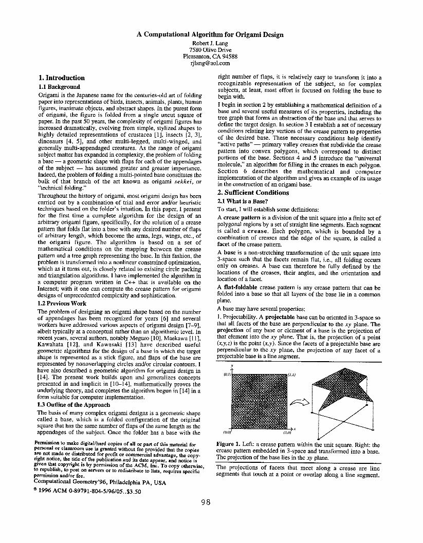
that all facets of the base are perpendicular to the xy plane. Theprojection of any base or element of a base is the projection ofthat element into the xy plane. That is, the projection of a point(x,Y,z) is the point (x,y). Since the facets of a protectable base areperpendicular to the xy plane, the projection of any facet of aprotectable base is a line segment.

Y

(o,

(o,

Figure 1. LefL a crease pattern within the unit square. Right: thecrease pattern embedded in 3-space and transformed into a base.The projection of the base lies in the xy plane.

The projections of facets that meet along a crease are linesegments that touch at a point or overlap along a line segment.

8

Since the facets of a crease pattern are connected, the set of allline segments formed by projecting individual facets into the xy

plane is connected as well and forms a planar embedding of a treegraph. The line segments thus formed are the edges of the graph;points where two edges come together are nodes of the graph.Nodes that have exactly one edge connected to them are terminalnodew the remaining nodes are internal nodes.

Definition: a flap k a group of facets in a base that project to acommon edge of the tree graph such that:

1. Every facet in the flap projects to the same edge;

2. Any facet in the base that projects to the edge and is connectedto a facet of the flap is itself a part of the flap.

3. The boundary of the facets that makeup the flap projects to oneor two nodes that are the endpoint(s) of the edge.

Therefore each flap in a base is associated with an edge of the treegraph. In many cases, the flaps of a protectable base can bepositioned at different angles, in 3-space giving projected treegraphs that differ in the arrangement of their edges. Note that twoside-by-side flaps may project to overlapping line segments in thev plane; we still distinguish different flaps by associating themwith distinct edges of the tree graph. To avoid ambiguity, a treegraph will always be drawn with nonoverlapping edges, but it

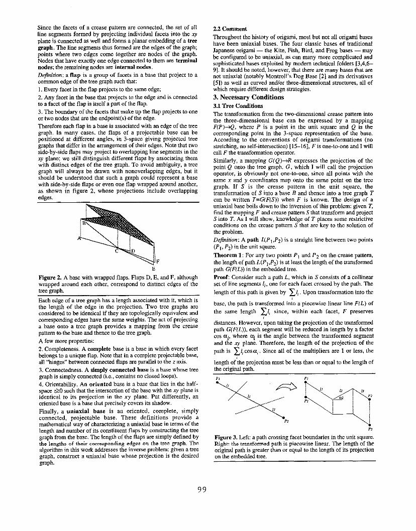
should be understood that such a graph could represent a basewith side-by-side flaps or even one flap wrapped around another,as shown in figure 2, whose projections include overlappingedges.

FE

Figure 2. A base with wrapped flaps. Flaps D, E, and F, althoughwrapped around each other, correspond to distinct edges of thetree graph.

Each edge of a tree graph has a length associated with it, which isthe length of the edge in the projection. Two tree graphs areconsidered to be identicrd if they are topologically equivalent andcorresponding edges have the same weights. The act of projectinga base onto a tree graph provides a mapping from the crease

pattern to the base and thence to the tree graph.

A few more properties:

2. Completeness. A complete base is a base in which every facetbelongs to a unique flap. Note that in a complete protectable base,rdl “hinges” between connected flaps are parallel to the z axis.

3. Connectedness. A simply connected base is a base whose treegraph is simply connected (i.e., contains no closed loops).

4. Orientability. An oriented base is a base that lies in the half-space z20 such that the intersection of the base with the w plane isidentical to its projection in the xy plane. Put differently, anoriented base is abase that precisely covers its shadow.

Finally, a uniaxial base is an oriented, complete, simplyconnected, protectable base. These definitions provide amathematicrd way of characterizing a uniaxial base in terms of thelength and number of its constituent flaps by constructing the treegraph from the base. The length of the flaps are simply defined bythe lengths of their corresponding edges on the tree graph. Thealgorithm in this work addresses the inverse problem: given a treegraph, construct a uniaxial base whose projection is the desiredgraph.

2.2 Comment

Throughout the history of origami, most but not all origami bases

have been uniaxial bases. The four classic bases of traditional

Japanese origami — the Kite, Fish, Bird, and Frog bases — maybe configured to be uniaxial, as can many more complicated andsophisticated bases exploited by modern technical folders [3,4,6–9]. It should be noted, however, that there are many bases that arenot uniaxial (notably Montroll’s Dog Base [2] and its derivatives[5]) as well as curved andlor three-dimensional structures, all ofwhich require different design strategies.

3. Necessary Conditions

3.1 Tree Conditions

The transformation from the two-dimensional crease pattern intothe three-dimensional base can be expressed by a mappingF(P)+, where F’ is a point in the unit square and Q is thecorresponding point in the 3-space representation of the base.According to the conventions of origami transformations (nostretching, no self-intersection) [15–1 6], F is one-to-one and I willcall F the transformation operator.

Similarly, a mapping G(Q)+R expresses the projection of thepoint Q onto the tree graph. G, which I will call the projectionoperator, is obviously not one-to-one, since all points with thesame x and y coordinates map onto the same point on the treegraph. If S is the crease pattern in the unit square, thetransformation of S into a base B and thence into a tree graph Tcan be written T= G(F(S)) when F is known. The design of auniaxial base boils down to the inversion of this problem: given T,find the mapping F and crease pattern S that transform and projectS into T. As I will show, knowledge of T places some restrictiveconditions on the crease pattern S that are key to the solution ofthe problem.

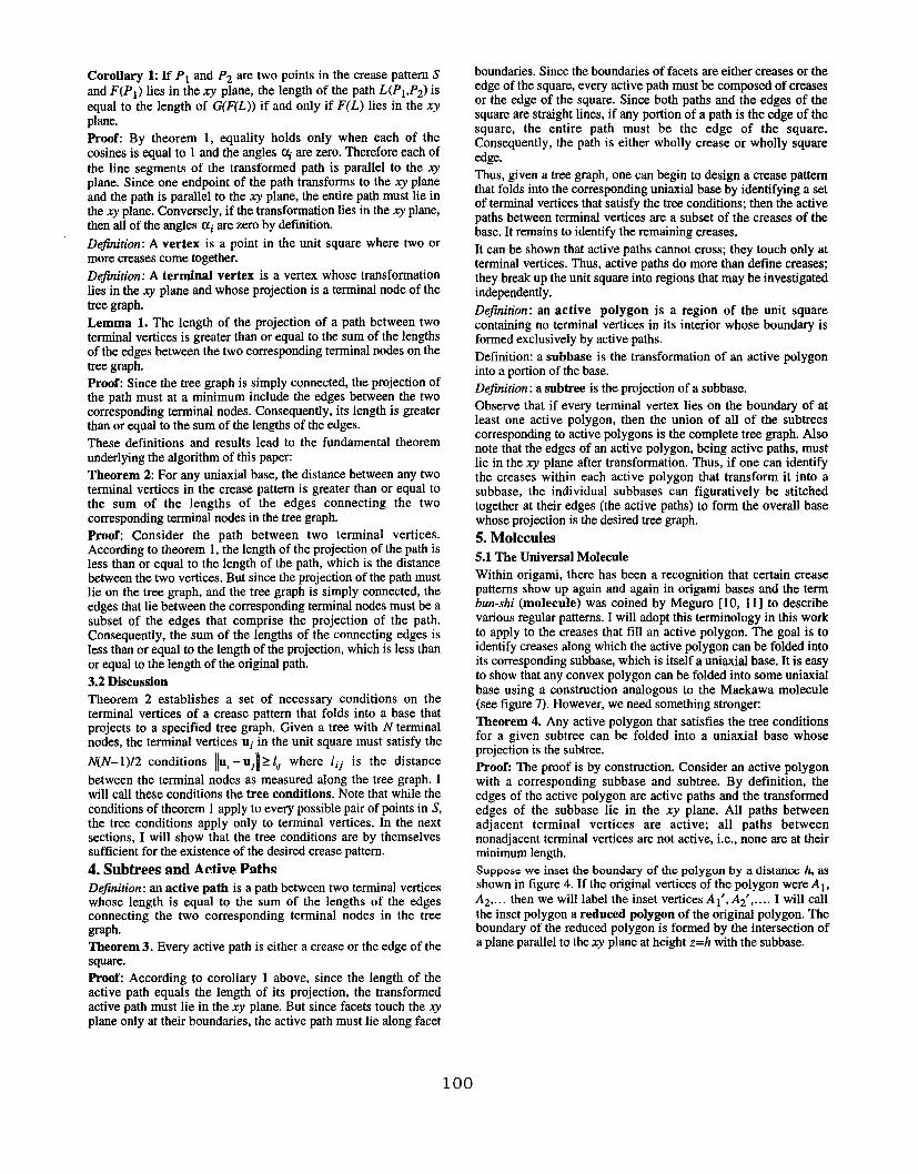
Definition: A path Z.(P1,P2) is a straight line between two points

(Pl, P2) in the unit square.

Theorem 1: For any two points P1 and P2 on the crease pattern,

the length of path L(P1,P2) is at least the length of the transformed

path G(F(L)) in the embedded tree.

Proof: Consider such a path L, which in S consists of a collinearset of line segments li, one for each facet crossed by the path. The

length of this path is given by xl,. Upon transformation into the

base, the uath is transformed into a uiecewise linear line F(L) of

the same length ~li since, within each facet, F preserves

distances. However, upon taking the projection of the transfon-nedpath G(F(L)), each segment will be reduced in length by a factor

cos rxti where ~ is the angle between the transformed segment

and the xy plane. Therefore, the length of the projection of the

path is Eli cos ai. Since all of the multipliers are 1 or less, the

length of the projection must be less than or equal to the length ofthe original path.

PI PI

P2

Figure 3. Left a path crossing facet boundaries in the unit square.Right, the transformed path is piecewise linear. The length of theoriginal path is greater than or equal to the length of its projectionon the embedded tree.

99

Corollary 1: If PI and P2 are two points in the crease pattern S

and F(P1) lies in the xy plane, the length of the path L(P1,P2) is

equal to the length of G(F(L)) if and only if F(L) lies in the xyplane.

Proof: By theorem 1, equality holds only when each of thecosines is equal to 1 and the angles cq are zero. Therefore each of

the line segments of the transformed path is parallel to the vplane. Since one endpoint of the path transforms to the xy planeand the path is parallel to the xy plane, the entire path must lie inthe xy plane. Conversely, if the transformation lies in the xy plane,then all of the angles ~i are zero by definition.

Definition: A vertex is a point in the unit square where two ormore creases come together.

Definition: A terminal vertex is a vertex whose transformation

lies in the xy plane and whose projection is a terminal node of thetree graph.

Lemma 1. The length of the projection of a path between twoterminal vertices is greater than or equal to the sum of the lengthsof the edges between the two corresponding terminal nodes on thetree graph.

Proof: Since the tree graph is simply connected, the projection ofthe path must at a minimum include the edges between the twocorresponding tertninrd nodes. Consequently. its length is greaterthan or equal to the sum of the lengths of the edges.

These definitions and results lead to the fundamental theoremunderlying the algorithm of this pape~

Theorem 2 For any tmiaxial base, the distance between any twoterminal vertices in the crease pattern is greater than or equal tothe sum of the lengths of the edges connecting the twocorresponding terminal nodes in the tree graph.

Proof: Consider the path between two terminal vertices.According to theorem 1, the length of the projection of the path isless than or equal to the length of the path, which is the distancebetween the two vertices. But since the projection of the path mustlie on the tree graph, and the tree graph is simply connected, theedges that lie between the corresponding terminal nodes must be asubset of the edges that comprise the projection of the path.Consequently, the sum of the lengths of the connecting edges isless than or equrd to the length of the projection, which is less thanor equal to the length of the original path.

3.2 Discussion

Theorem 2 establishes a set of necessary conditions on theterminal vertices of a crease pattern that folds into a base thatprojects to a specified tree graph. Given a tree with N terminalnodes, the terminal vertices ui in the unit square must satisfy the

N(N-1)12 conditions I/u, - u,]] 21,, where lij is the distance

between the terminal nodes as measured along the tree graph. Iwill call these conditions the tree conditions. Note that while theconditions of theorem 1 apply to every possible pair of points in S,the tree conditions apply only to terminal vertices. In the nextsections, I will show that the tree conditions are by themselvessufficient for the existence of the desired crease pattern.

4. Subtrees and Active Paths

Definition: an active path is a path between two terminal verticeswhose length is equal to the sum of the lengths of the edgesconnecting the two corresponding terminal nodes in the treegraph.

Theorem 3. Every active path is either a crease or the edge of thesquare.

Proof: According to corollary 1 above, since the length of theactive path equals the length of its projection, the transformedactive path must lie in the xy plane. But since facets touch the xyplane only at their boundaries, the active path must lie rdong facet

boundaries. Since the boundaries of facets are either creases or theedge of the square, every active path must be composed of creasesor the edge of the square. Since both paths and the edges of thesquare are straight lines, if any portion of a path is the edge of thesquare, the entire path must be the edge of the square.Consequently, the path is either wholly crease or wholly squareedge.

Thus, given a tree graph, one can begin to design a crease patternthat folds into the corresponding trniaxird base by identifying a setof terminal vertices that satisfy the tree conditions; then the activepaths between terminal vertices are a subset of the creases of thebase. It remains to identify the remaining creases.

It can be shown that active paths cannot cross; they touch only atterminal vertices. Thus, active paths do more than define creases;they break up the unit square into regions that maybe investigatedindependently.

De~nition: an active polygon is a region of the unit squarecontaining no terminal vertices in its interior whose boundary isfortned exclusively by active paths.

Definition: a subbase is the transformation of an active polygoninto a portion of the base.

Definition: a aubtree is the projection of a subbase.

Observe that if every terminal vertex lies on the boundary of atleast one active polygon, then the union of all of the subtrees

corresponding to active polygons is the complete tree graph. Alsonote that the edges of an active polygon, being active paths, mustlie in the xy plane after transformation. Thus, if one can identifythe creases within each active polygon that transform it into asubbase, the individual subbases can figuratively be stitchedtogether at their edges (the active paths) to form the overall basewhose projection is the desired tree graph.

5. Molecules

5.1 The Universal Molecule

Within origami, there has been a recognition that certain creasepatterns show up again and again in origami bases and the termbun-shi (molecule) was coined by Megtrro [10, 11] to describevarious regular patterns. I will adopt this terminology in this workto apply to the creases that fill an active polygon. The gord is toidentify creases along which the active polygon can be folded intoits corresponding subbase, which is itself a tmiaxial base. It is easyto show that any convex polygon can be folded into some uniaxialbase using a construction analogous to the Maekawa molecule(see figure 7). However, we need something stronge~

Theorem 4. Any active polygon that satisfies the tree conditionsfor a given subtree can be folded into a uniaxial base whoseprojection is the subtree.

ProoE The proof is by construction. Consider an active polygonwith a corresponding subbase and subtree. By definition, theedges of the active polygon are active paths and the transformededges of the subbase lie in the xy plane. All paths betweenadj scent terminal vertices are active; all paths betweennonadjacent terminal vertices are not active, i.e., none are at theirminimum length.

Suppose we inset the boundary of the polygon by a distance h, asshown in figure 4. If the original vertices of the polygon were A 1,

A2,... then we will label the inset vertices A 1’, A2’, . . . . I will call

the inset polygon a reduced polygon of the original polygon. Theboundary of the reduced polygon is formed by the intersection ofa plane parallel to the xy plane at height z=h with the subbase.

100

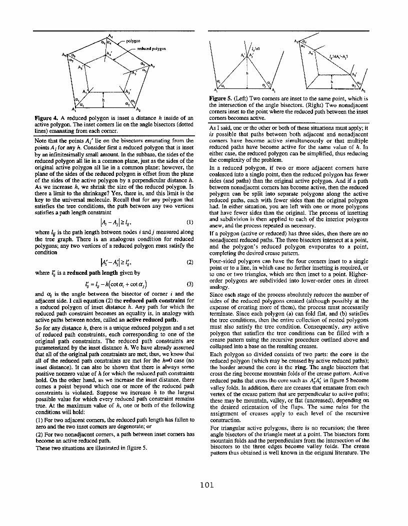
Figure 4. A reduced polygon is inset a distance h inside of anactive polygon. The inset comers lie on the angle bisectors (dottedlines) emanating from each comer.

Note that the points Ai’ lie on the bisectors emanating from the

points Ai for any h. Consider first a reduced polygon that is insetby an infinitesimally smrdl amount. In the subbase, the sides of thereduced polygon all lie in a common plane, just as the sides of theoriginal active polygon rdl lie in a common plane; however, theplane of the sides of the reduced polygon is offset from the planeof the sides of the active polygon by a perpendicular distance h.As we increase h, we shrink the size of the reduced polygon. Isthere a limit to the shrinkage? Yes, there is, and this limit is thekey to the universal molecule. Recall that for any polygon thatsatisfies the tree conditions, the path between any two verticessatisfies a path length constraint

IA, -AJ21,, (1)

where Iv is the path length between nodes i and j measured along

the tree graph. There is an analogous condition for reducedpolygons; any two vertices of a reduced polygon must satisfy thecondition

where l; is a reduced path length given by

1;= lU - h(cot a, + cot et,)

(2)

(3)

and cq is the angle between the bisector of corner i and the

adjacent side. I call equation (2) the reduced path constraint fora reduced polygon of inset distance h. Any path for which thereduced path constraint becomes an equality is, in analogy withactive paths between nodes, called an active reduced path.

So for any distance h, there is a unique reduced polygon and a set

of reduced path constraints, each corresponding to one of theoriginal path constraints. The reduced path constraints areparametrized by the inset distance h. We have already assumedthat all of the original path constraints are met thus, we know thatall of the reduced path constraints are met for the h=O case (noinset distance). It can also be shown that there is always somepositive nonzero vahre of h for which the reduced path constraintshold. On the other hand, as we increase the inset distance, therecomes a point beyond which one or more of the reduced pathconstraints is violated. Suppose we increase h to the largestpossible value for which every reduced path constraint remainstrue. At the maximum value of h, one or both of the followingconditions will hold:

(1) For two adjacent comers, the reduced path length has fallen tozero and the two inset comers are degenerate, or

(2) For two nonadjacent comers, a path between inset comers hasbecome an active reduced path.

These two situations are illustrated in figure 5.

!kA!!!J1

Figure 5. (Left) Two comers are inset to the same point, which isthe intersection of the angle bisectors. (Right) Two nonadjacentcomers inset to the point where the reduced path between the insetcomers becomes active.

As I said, one or the other or both of these situations must apply; itis possible that paths between both adjacent and nonadjacentcorners have become active simultaneously or that multiplereduced paths have become active for the same value of h. Ineither case, the reduced polygon can be simplified, thus reducing

the complexity of the problem.

In a reduced polygon, if two or more adjacent comers havecoalesced into a single point, then the reduced polygon has fewersides (and paths) than the original active polygon. And if a pathbetween nonadjacent comers has become active, then the reducedpolygon can be split into separate polygons along the activereduced paths, each with fewer sides than the original polygonhad. In either situation, you are left with one or more polygonsthat have fewer sides than the original. The process of insettingand subdivision is then applied to each of the interior polygonsanew, and the process repeated as necessay.

If a polygon (active or reduced) has three sides, then there are nononadjacent reduced paths. The three bisectors intersect at a point,and the polygon’s reduced polygon evaporates to a point,completing the desired crease pattern.

Four-sided polygons can have the four corners inset to a singlepoint or to a line, in which case no further insetting is required, orto one or two triangles, which are then inset to a point. Higher-order polygons are subdivided into lower-order ones in directanalogy.

Since each stage of the process absolutely reduces the number ofsides of the reduced polygons created (although possibly at theexpense of creating more of them), the process must necessarilyterminate. Since each polygon (a) can fold flat, and (b) satisfiesthe tree conditions, then the entire collection of nested polygonsmust also satisfy the tree condition. Consequently, any activepolygon that satisfies the tree conditions can be filled with a

crease pattern using the recursive procedure outlined above andcollapsed into abase on the resulting creases.

Each polygon so divided consists of two parts: the core is thereduced polygon (which may be crossed by active reduced paths);the border around the core is the ring. The angle bisectors thatcross the ring become mountain folds of the crease pattern. Active

reduced paths that cross the core such as AjAj in figure 5 become

valley folds. In addition, there are creases that emanate from eachvertex of the crease pattern that are perpendicular to active paths;these may be mountain, valley, or flat (ungreased), depending onthe desired orientation of the flaps. The same rules for theassignment of creases apply to each level of the recursive

construction.

For triangular active polygons, there is no recursion; the threeangle bisectors of the triangle meet at a point. The bisectors formmountain folds and the perpendiculars from the intersection of thebisectors to the three edges become valley folds. The creasepattern thus obtained is well known in the origami literature. The

101

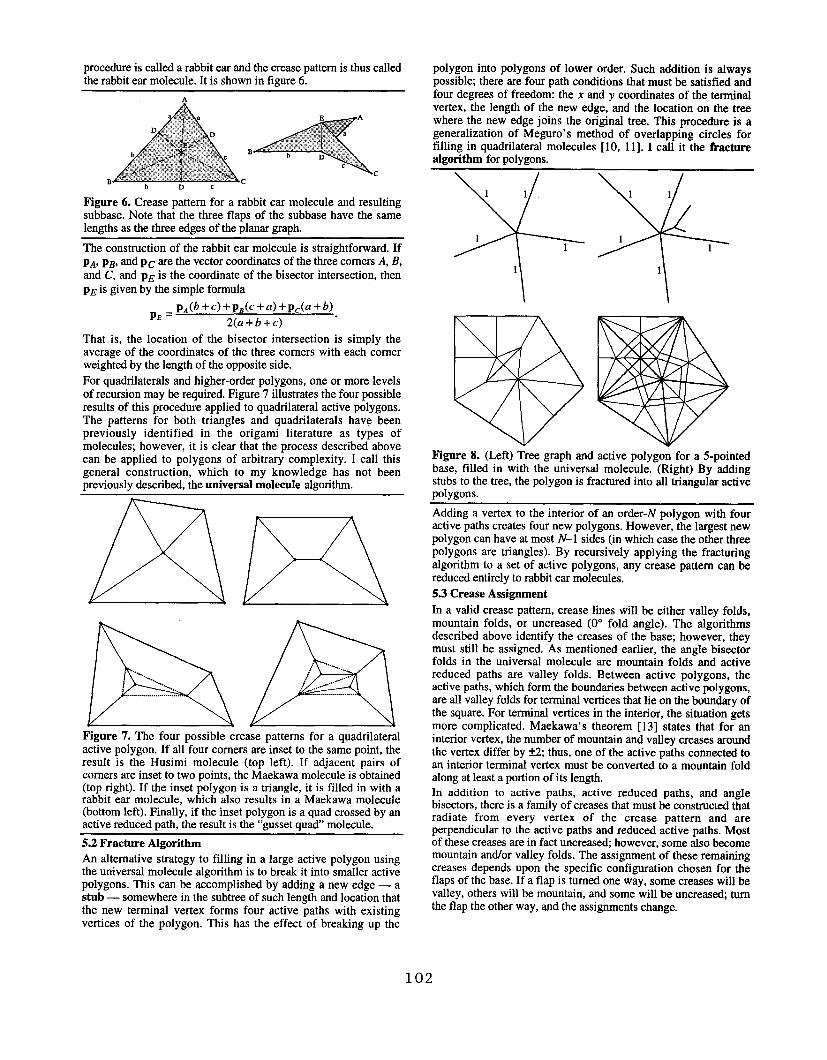
procedure is called a rabbit ear and the crease pattern is thus called

the rabbit ear molecule. It is shown in figure 6.

Figure 6. Crease pattern for a rabbit ear molecule and resultingsubbase. Note that the three flaps of the subbase have the samelerwths as the three edges of the danar zraDh.

The construction of the rabbit ear molecule is straightforward. If

PA, PB, ~d PC Me the vector coordinates of the three comers A, B>and C, and pE is the coordinate of the bisector intersection, then

pE is given by the simple formula

pE = P.(b +C)+PB(c+a)+Pc(a +b)2(a+b+c)

.

That is, the location of the bisector intersection is simply theaverage of the coordinates of the three comers with each comerweighted by the length of the opposite side.

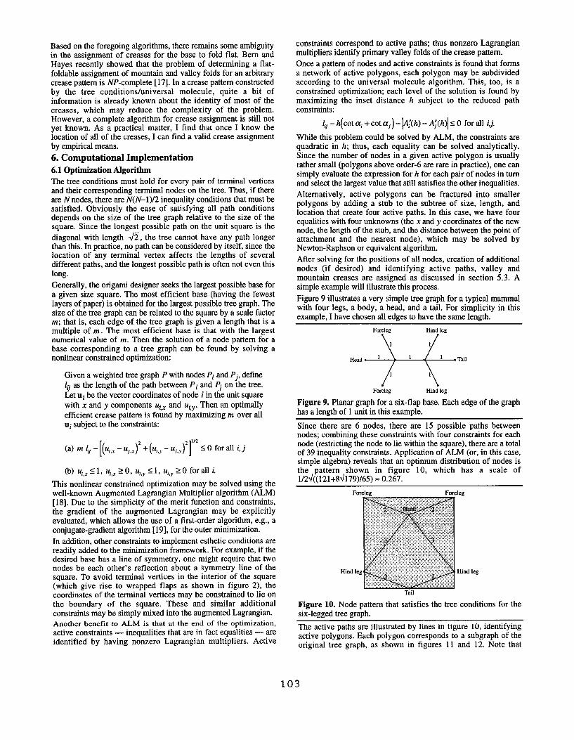
For quadrilaterals and higher-order polygons, one or more levels

of recursion maybe required. Figure 7 illustrates the four possibleresults of this procedure applied to quadrilateral active polygons.The patterns for both triangles and quadrilaterals have beenpreviously identified in the origami literature as types ofmolecules; however, it is clear that the process described abovecan be applied to polygons of arbitrary complexity. I call thisgeneral construction, which to my knowledge has not beenpreviously described, the universal molecule algorithm.

k&Figure 7. The four possible crease patterns for a quadrilateralactive polygon. If all four comers are inset to the same point, theresult is the Husimi molecule (top left). If adjacent pairs ofcomers are inset to two points, the Maekawa molecule is obtained(top right). If the inset polygon is a triangle, it is filled in with arabbit ear molecule, which also results in a Maekawa molecule(bottom left). Finally, if the inset polygon is a quad crossed by anactive reduced path, the result is the “gusset quad” molecule.

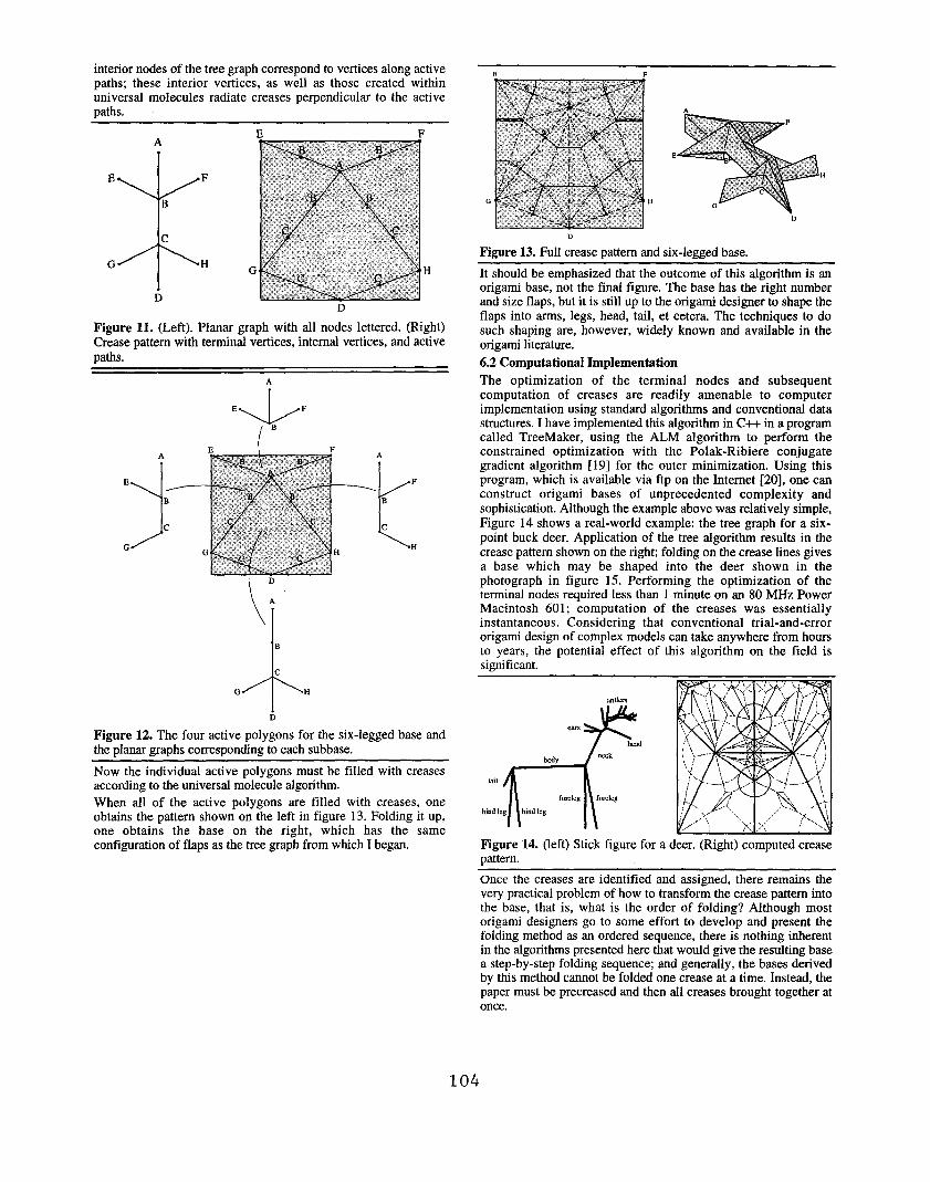
5.2 Fracture Algorithm

An alternative strategy to filling in a large active polygon usingthe universrd molecule algorithm is to break it into smaller activepolygons. This can be accomplished by adding a new edge — astub — somewhere in the subtree of such length and location that

the new terminal vertex forms four active paths with existingvertices of the polygon. This has the effect of breaking up the

polygon into polygons of lower order. Such addition is alwayspossible; there are four path conditions that must be satisfied andfour degrees of freedom: the x and y coordinates of the terminalvertex, the length of the new edge, and the location on the treewhere the new edge joins the original tree. This procedure is ageneralization of Megttro’s method of overlapping circles forfilling in quadrilateral molecules [10, 11]. I call it the fracturealgorithm for polygons.

+

1 1

11

1

Figure 8. (Left) Tree graph and active polygon for a 5-pointedbase, filled in with the universal molecule. (Right) By addingstubs to the tree, the polygon is fractured into all triangular active

~olv~ons.

Adding a vertex to the interior of an order-N polygon with fouractive paths creates four new polygons. However, the largest newpolygon can have at most N-1 sides (in which case the other threepolygons are triangles). By recursively applying the fracturingrdgorithm to a set of active polygons, any crease pattern can bereduced entirely to rabbit ear molecules.

5.3 Crease Assignment

In a valid crease pattern, crease lines will be either valley folds,mountain folds, or uncreased (0° fold angle). The rdgorithmsdescribed above identify the creases of the base; however, theymust still be assigned. As mentioned earlier, the angle bisectorfolds in the universal molecule are mountain folds and activereduced paths are valley folds. Between active polygons, theactive paths, which form the boundaries between active polygons,are all valley folds for terminal vertices that lie on the boundary ofthe square. For terminal vertices in the interior, the situation getsmore complicated. Maekawa’s theorem [13] states that for aninterior vertex, the number of mountain and valley creases around

the vertex differ by&; thus, one of the active paths connected toan interior terminal vertex must be converted to a mountain foldalong at least a portion of its length.

In addition to active paths, active reduced paths, and anglebisectors, there is a family of creases that must be constructed thatradiate from every vertex of the crease pattern and areperpendicular to the active paths and reduced active paths. Mostof these creases are in fact uncreased; however, some also becomemountain and/or valley folds. The assignment of these remainingcreases depends upon the specific configuration chosen for theflaps of the base. If a flap is turned one way, some creases will bevalley, others will be mountain, and some will be uncreased; turnthe flap the other way, and the assignments change.

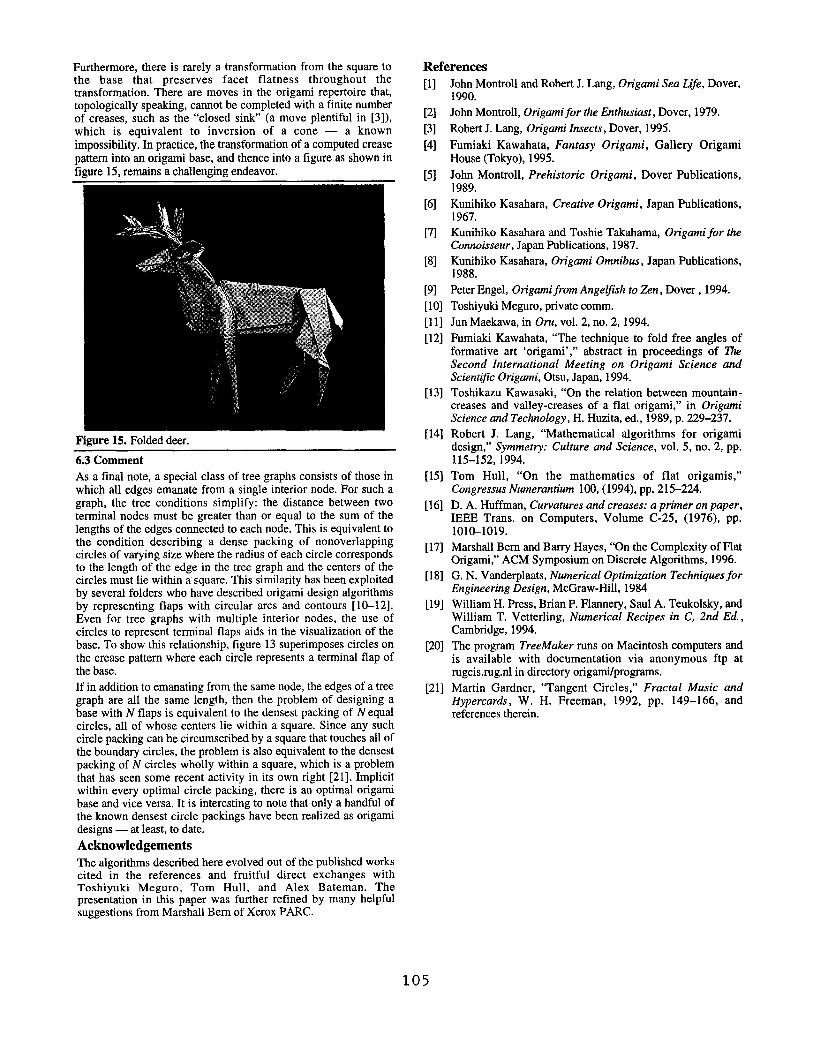
1102

Based on the foregoing algorithms, there remains some ambiguityin the assignment of creases for the base to fold flat. Bern and

Hayes recently showed that the problem of determining a flat-foldable assignment of mountain and valley folds for an arbitrarycrease pattern is NP-complete [17]. In a crease pattern constructed

by the tree conditions/universal molecule, quite a bit ofinformation is already known about the identity of most of thecreases, which may reduce the complexity of the problem.However, a complete algorithm for crease assignment is still notyet known. As a practical matter, I find that once I know thelocation of all of the creases, I can find a valid crease assignmentby empiricrd means.

6. Computational Implementation

6.1 Optimization Algorithm

The tree conditions must hold for every pair of terminal verticesand their corresponding terminal nodes on the tree. Thus, if thereare N nodes, there are N(N-1 )/2 inequality conditions that must besatisfied. Obviously the ease of satisfying all path conditionsdepends on the size of the tree graph relative to the size of thesquare. Since the longest possible path on the unit square is the

diagonal with length W, the tree cannot have any path longerthan this. In practice, no path can be considered by itself, since thelocation of any terminal vertex affects the lengths of severaldifferent paths, and the longest possible path is often not even thislong.

Generally, the origami designer seeks the largest possible base for

a given size square. The most efficient base (having the fewestlayers of paper) is obtained for the largest possible tree graph. Thesize of the tree graph can be related to the square by a scale factorm; that is, each edge of the tree graph is given a length that is amultiple of m. The most efficient base is that with the largestnumerical value of m. Then the solution of a node pattern for abase corresponding to a tree graph can be found by solving anonlinear constrained optimization:

Given a weighted tree graph P with nodes Pi and Pj, define

ld as the length of the path between Pi and Pj on the tree.

Let ui be the vector coordinates of node i in the unit square

with x and y components ui,x and Ui,y. Then an optimally

efficient crease pattern is found by maximizing m over allui subject to the constraints:

[(s0 m lU- (u/,x- u],=~+(ui,~-uj,~~l’” SO for all i,j

(b) U,,XS1, u,,, 20, U,,YS1, ui,Y20 for all i.

This nonlinear constrained optimization may be solved using thewell-known Augmented Lagrangian Multiplier algorithm (ALM)[18]. Due to the simplicity of the merit function and constraints,the gradient of the augmented Lagrangian may be explicitly

evahtated, which allows the use of a first-order algorithm, e.g., aconjugate-gradient algorithm [19], for the outer minimization.

In addition, other constraints to implement esthetic conditions arereadily added to the minimization framework. For example, if thedesired base has a line of symmetry, one might require that twonodes be each other’s reflection about a symmetry line of thesquare. To avoid terminal vertices in the interior of the square(which give rise to wrapped flaps as shown in figure 2), thecoordinates of the terminal vertices may be constrained to lie onthe boundary of the square. These and similar additionalconstraints may be simply mixed into the augmented Lagrangirm.

Another benefit to ALM is that at the end of the optimization,active constraints — inequalities that are in fact equalities — areidentified by having nonzero Lagrangian multipliers. Active

constraints correspond to active paths; thus nonzero Lagrangianmultipliers identify primary valley folds of the crease pattern.

Once a pattern of nodes and active constraints is found that formsa network of active polygons, each polygon may be subdividedaccording to the universal molecule algorithm. This, too, is a

constrained optimizatiorv each level of the solution is found bymaximizing the inset distance h subject to the reduced pathconstraints:

11– h(cot a, + cot a,) – lAJ(h) - Aj(h)ls O for all i,j.

While this problem could be solved by ALM, the constraints arequadratic in h; thus, each equality can be solved analytically.Since the number of nodes in a given active polygon is usuallyrather smrdl (polygons above order-6 are rare in practice), one cansimply evahtate the expression for h for each pair of nodes in turnand select the largest value that still satisfies the other ineqttrdities.

Alternatively, active polygons can be fractured into smallerpolygons by adding a stub to the subtree of size, length, andlocation that create four active paths. In this case, we have fourequalities with four unknowns (the x and y coordinates of the newnode, the length of the stub, and the distance between the point ofattachment and the nearest node), which may be solved byNewton-Raphson or equivalent rdgorithm.

After solving for the positions of all nodes, creation of additionrdnodes (if desired) and identifying active paths, valley and

mountain creases are assigned as discussed in section 5.3. Asimple example will illustrate this process.

Figure 9 illustrates a very simple tree graph for a typical mammalwith four legs, a body, a head, and a tail. For simplicity in thisexample, I have chosen all edges to have the same length.

Foreleg*

Hhd legP

J \Foreles Hind Ies

Figure 9. Planar graph for a six-flap base. Each edge of the graphhas a length of 1 unit in this example.

Figure 10. Node pattern that satisfies the tree conditions for thesix-legged tree graph.

The active paths are illustrated by lines in figure 10, identifyingactive polygons. Each polygon corresponds to a subgraph of theoriginal tree graph, as shown in figures 11 and 12. Note that

103

interior nodes of the tree graph correspond to vertices along activepaths; these interior vertices, as well as those created withinuniversal molecules radiate creases perpendicular to the activepaths.

A

D

Figure 11. (Left). Planar graph with all nodes lettered. (Right)Crease pattern with terminal vertices, internal vertices, and active

paths.

A

E

J/

F

1°

4“\

B

c

G H

D

Figure 12. The four active polygons for the six-legged base andthe planar graphs corresponding to each subbase.

Now the individual active polygons must be filled with creasesaccording to the universal molecule algorithm.

When all of the active polygons are filled with creases, oneobtains the pattern shown on the left in figure 13. Folding it up,one obtains the base on the right, which has the sameconfiguration of flaps as the tree graph from which I began.

D

Figure 13. Full crease pattern and six-legged base.

It should be emphasized that the outcome of this algorithm is anorigami base, not the final figure. The base has the right numberand size flaps, but it is still up to the origami designer to shape theflaps into arms, legs, head, tail, et cetera. The techniques to dosuch shaping are, however, widely known and available in theorigami literature.

6.2 Computational Implementation

The optimization of the terminal nodes and subsequentcomputation of creases are readily amenable to computerimplementation using standard algorithms and conventional datastructures. I have implemented this algorithm in C++ in a programcalled TreeMaker, using the ALM algorithm to perform theconstrained optimization with the Polak-Ribiere conjugategradient algorithm [19] for the outer minimization. Using thisprogram, which is available via ftp on the Intemet [20], one canconstruct origami bases of unprecedented complexity and

sophistication. Although the example above was relatively simple,Figure 14 shows a real-world example: the tree graph for a six-point buck deer. Application of the tree algorithm results in thecrease pattern shown on the righ~ folding on the crease lines givesa base which may be shaped into the deer shown in thephotograph in figure 15. Performing the optimization of theterminal nodes required less than 1 minute on an 80 MHz PowerMacintosh 601; computation of the creases was essentiallyinstantaneous. Considering that conventional trial-and-errororigami design of complex models can take anywhere from hoursto years, the potential effect of this algorithm on the field issignificant. -

ankx

emsF head

M.neck

n....mil

foreleg fmekg

hind leg hid leg

. .[/ /’-’

r. ,<..,4/\,.>.,

i ,, ,, \

Figure 14. (left) Stick figure for a deer. (Right) computed creasepattern.

Once the creases are identified and assigned, there remains thevery practical problem of how to transform the crease pattern intothe base, that is, what is the order of folding? Although mostorigami designers go to some effort to develop and present thefolding method as an ordered sequence, there is nothing inherentin the algorithms presented here that would give the resulting basea step-by-step folding sequence; and generally, the bases derivedby this method cannot be folded one crease at a time. Instead, thepaper must be precreased and then all creases brought together atonce.

104

References

6.3 Comment

As a final note, a special class of tree graphs consists of those inwhich all edges emanate from a single interior node. For such agraph, the tree conditions simplify: the distance between twoterminal nodes must be greater than or equal to the sum of the

lengths of the edges connected to each node. This is equivalent tothe condition describing a dense packing of nonoverlappingcircles of varying size where the radius of each circle correspondsto the length of the edge in the tree graph and the centers of thecircles must lie within a square. This similarity has been exploitedby several folders who have described origami design algorithmsby representing flaps with circular arcs and contours [10-12].Even for tree graphs with multiple interior nodes, the use of

circles to represent terminal flaps aids in the visualization of thebase. To show this relationship, figure 13 superimposes circles onthe crease pattern where each circle represents a terminal flap ofthe base.

If in addition to emanating from the same node, the edges of a treegraph are all the same length, then the problem of designing a

base with N flaps is equivalent to the densest packing of N equalcircles, all of whose centers lie within a square. Since any suchcircle packing can be circumscribed by a square that touches all ofthe boundary circles, the problem is also equivalent to the densestpacking of N circles wholly within a square, which is a problem

that has seen some recent activity in its own right [21]. Implicitwithin every optimal circle packing, there is an optimal origami

base and vice versa. It is interesting to note that only a handful ofthe known densest circle packings have been realized as origamidesigns — at least, to date.

Acknowledgements

[1]

[2]

[3]

[4]

[5]

[6]

[m

[8]

[9]

[10]

[11]

[12]

[13]

[14]

[15]

[16]

[17]

[18]

[19]

[20]

[21]

John Montroll and Robert J. Lang, Origami Sea Life, Dover,1990.

John Montroll, Origami for the Enthusiast, Dover, 1979.

Robert J. Lang, Origami Insects, Dover, 1995.

Fumiaki Kawahata, Fantasy Origami, Gallery Origami

House (Tokyo), 1995.

John Montroll, Prehistoric Origami, Dover Publications,1989.

Kunihiko Kasahara, Creative Origami, Japan Publications,1967.

Kunihiko Kasahara and Toshie Takahama, Origami for theConnoisseur, Japan Publications, 1987.

Kunihiko Kasahara, Origami Omnibus, Japan Publications,1988.

Peter Engel, Origamifiom Angeljish to Zen, Dover, 1994.

Toshiyuki Meguro, private comm.

Jun Maekawa, in Oru, vol. 2, no, 2, 1994.

Fumiaki Kawahata, “The technique to fold free angles offormative art ‘origami’ ~’ abstract in proceedings of TheSecond International Meeting on Origami Science andScientljic Origami, Otsu, Japan, 1994.

Toshikazu Kawasaki, “On the relation between mountain-creases and valley-creases of a flat origami,” in OrigamiScience and Technology, H. Huzita, cd., 1989, p. 229-237.

Robert J. Lang, “Mathematical algorithms for origami

designl’ Symmetry: Culture and Science, vol. 5, no. 2, pp.115-152,1994.

Tom Hull, “On the mathematics of flat origamis,”Congresses Numerantium 100, (1994), pp. 215-224.

D. A. Huffman, Curvatures and creases: a primer on paper,IEEE Trans. on Computers, Volume C-25, (1976), pp.

1010-1019.

Marshall Bern and Barry Hayes, “On the Complexity of FlatOrigami,” ACM Symposium on Discrete Algorithms, 1996.

G. N. Vanderplaats, Numerical Optimization Techniques forEngineering Design, McGraw-Hill, 1984

William H. Press, Brian P. Flannery, Saul A. Teukolsky, andWilliam T. Vetterling, Numerical Recipes in C, 2nd Ed.,Cambridge, 1994.

The program TreeMaker runs on Macintosh computers andis available with documentation via anonymous ftp atrugcis.rug,nl in directory origami/programs.

Martin Gardner, “Tangent Circles,” Fractal Music andHyperCard, W. H. Freeman, 1992, pp. 149-166, andreferences therein.

The algorithms described here evolved out of the published workscited in the references and fruitful direct exchanges withToshiyuki Meguro, Tom Hull, and Alex Bateman. Thepresentation in this paper was further refined by many helpfulsuggestions from Marshall Bern of Xerox PARC.

105