a comparative study between priority assigning method...

- 1 -

A COMPARATIVE STUDY BETWEEN PRIORITY ASSIGNING

METHOD AND LAMBDA ITERATION METHOD FOR UNIT

COMMITMENT PROBLEMS

CHANDAN BHARDWAJ (109EE0034)

MAYANK MISHRA (109EE0047)

Department of Electrical Engineering

National Institute of Technology Rourkela

- 2 -

A COMPARATIVE STUDY BETWEEN PRIORITY

ASSIGNING METHOD AND LAMBDA ITERATION

METHOD FOR UNIT COMMITMENT PROBLEMS

A Thesis submitted in partial fulfillment of the requirements for the degree of

Bachelor of Technology in “Electrical Engineering”

By

CHANDAN BHARDWAJ (109EE0034)

MAYANK MISHRA (109EE0047)

Under guidance of

Prof. Sanjib Ganguly

Department of Electrical Engineering

National Institute of Technology

Rourkela-769008 (ODISHA)

May-2013

- 3 -

DEPARTMENT OF ELECTRICAL ENGINEERING

NATIONAL INSTITUTE OF TECHNOLOGY, ROURKELA

ODISHA, INDIA-769008

CERTIFICATE

This is to certify that the thesis entitled “A Comparative Study Between Priority Assigning

Method And Lambda Iteration Method for Unit Commitment Problems”, submitted Mr.

Chandan Bhardwaj, Roll No: 109EE0034 and Mr. Mayank Mishra, Roll No: 109EE0047 in

partial fulfilment of the requirements for the award of Bachelor of Technology in Electrical

Engineering during session 2010-2011 at National Institute of Technology, Rourkela. A

bonafide record of research work carried out by them under my supervision and guidance.

The candidates have fulfilled all the prescribed requirements.

The Thesis which is based on candidates‟ own work, have not submitted elsewhere for a

degree/diploma.

In my opinion, the thesis is of standard required for the award of a bachelor of technology degree

in Electrical Engineering.

Place: Rourkela

Dept. of Electrical Engineering Prof. Sanjib Ganguly

National institute of Technology Supervisor

Rourkela-769008

a

ACKNOWLEDGEMENTS

We wish to express our sincere gratitude to our guide Prof. Sanjib Ganguly Electrical Engineering

Department, National Institute of Technology, Rourkela for his invaluable guidance and co-operation, and

for providing the necessary facilities and sources during the period of this project. We would also like to

thank the authors of various research articles and books that we referred to during the course of the

project.

Chandan Bhardwaj

Mayank Mishra

B.Tech (Electrical Engineering)

2

ABSTRACT

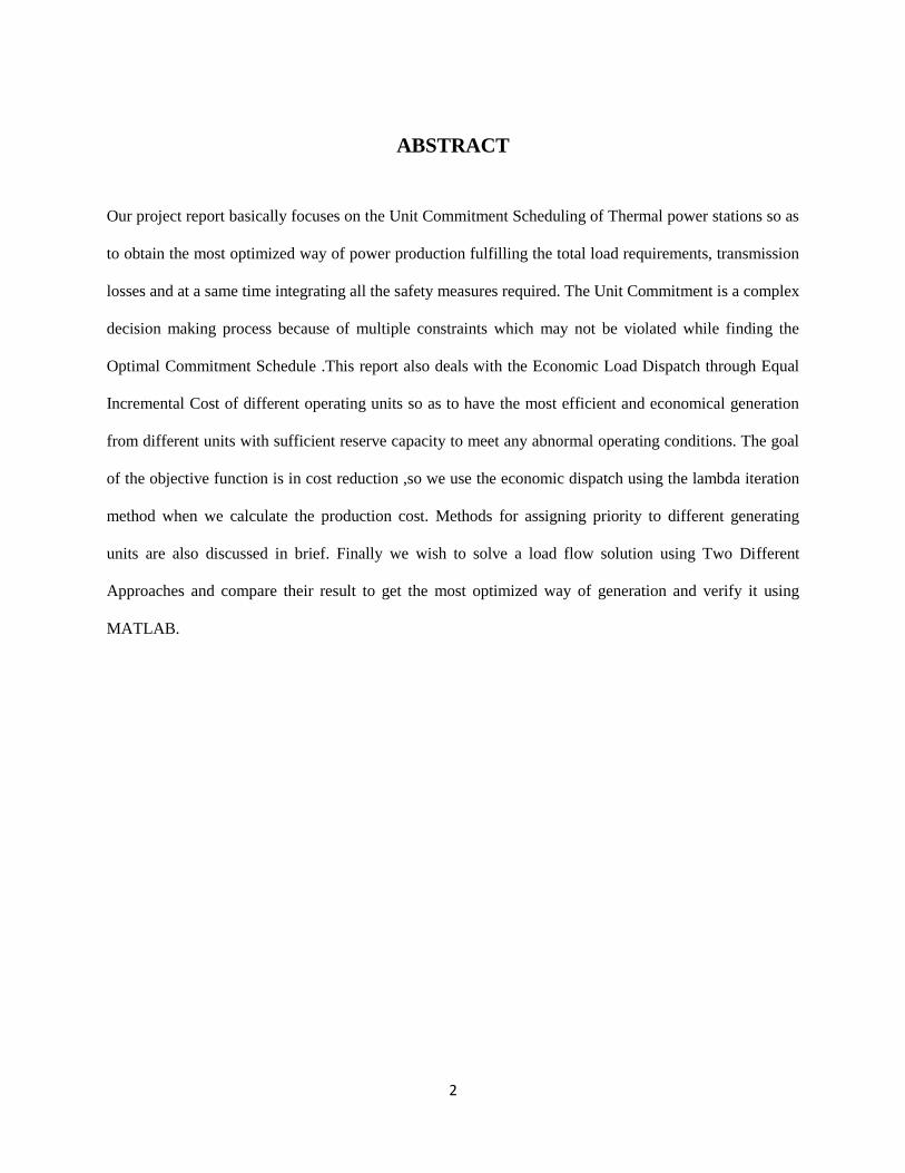
Our project report basically focuses on the Unit Commitment Scheduling of Thermal power stations so as

to obtain the most optimized way of power production fulfilling the total load requirements, transmission

losses and at a same time integrating all the safety measures required. The Unit Commitment is a complex

decision making process because of multiple constraints which may not be violated while finding the

Optimal Commitment Schedule .This report also deals with the Economic Load Dispatch through Equal

Incremental Cost of different operating units so as to have the most efficient and economical generation

from different units with sufficient reserve capacity to meet any abnormal operating conditions. The goal

of the objective function is in cost reduction ,so we use the economic dispatch using the lambda iteration

method when we calculate the production cost. Methods for assigning priority to different generating

units are also discussed in brief. Finally we wish to solve a load flow solution using Two Different

Approaches and compare their result to get the most optimized way of generation and verify it using

MATLAB.

3

Table of Contents

Abstract……………………………………………………………………………………………2

Contents…………………………………………………………………………………………...3

List of Figures……………………………………………………………………………………..5

List of Tables……………………………………………………………………………………...6

CHAPTER 1:

UNIT COMMITMENT

1.1 INTRODUCTION, WHAT IS UNIT COMMITMENT…………………………….............................8

1.2 APPLICATIONS OF UNIT COMMITMENT ………………………………………………………..8

1.3 LITERATURE REVIEW……………………………………………………………………………....9

CHAPTER 2:

ECONOMICS OF POWER GENERATION

2.1 ECONOMICS OF POWER GENERATION……………………………………………………...….14

2.2 THERMAL GENERATION…………………………………………………………………………..15

2.3 CONSTRAINTS……………………………………………………………………...……………….16

CHAPTER 3:

METHODS OF UNIT COMMITMENT

3.1 METHODS OF UNIT COMMITMENT………………………………………………………….…..19

3.1.1 Introduction……………………………………………………………………………...….19

3.1.2 A major setback to this method………………………………………..................................19

3.2 A MODIFIED APPROACH METHOD OF EQUAL INCREMENT……………………….………..21

3.2.1 Introduction………………………………………………………………………………....21

3.2.2 Advantage of this method……………………………………………………..……………22

3.2.3 Drawback of this method………………………………………………………………...…22

3.2.4 Flowchart representation of this method……………………………………………………23

4

3.3 LAMDA ITERATIVE METHOD……………………………………………………...……………..24

3.3.1 Hit and trial method…………………………………………………………….…………....24

3.3.2 Regular falsi method…………………………………………………………………………24

3.4 PRIORITY LIST APPROACH FOR ECONOMIC LOAD DISPATCH……………………………..26

3.4.1 Introduction ………………………………………………………………….………………26

3.4.2 Flowchart representation of this method……………………………………...…………….. 27

CHAPTER 4:

RESULTS AND DISCUSSIONS

4.1 LOAD CURVE ……………………………………………………………………………………….29

4.2 UNIT CHARACTERISTICS ………………………………………………………...……………….30

4.3 RESULTS OBTAINED BY MODIFIED EQUAL INCREMENTAL PRODUCTION COST

(METHOD1)…………………………………………………………………………………………..….31

4.3.1 Generation graph of various generators……………………………………………...…………32

4.3.2 Graph showing the variation of lambda………………………………………………..……….33

4.4 RESULTS OBTAINED BY PRIORITY ASSIGNING METHOD (METHOD 2)…………………..34

4.5 COMPARATIVE STUDY……………………………………………………………………………35

CHAPTER 5:

CONCLUSION

5.1 Conclusion……………………………………………………………….………………………….38

REFERENCE ………………………………………………………………………..…………………..39

5

LIST OF FIGURES

S. No TITLE PAGE NO

3.1 FLOW CHART REPRESENTATION OF MODIFIED EQUAL

INCREMENATL PRODUCTION COST METHOD

23

3.2 LAMBDA ITERATION BY REGULA-FALSI METHOD 25

3.3 FLOW CHART REPRESENTATION OF PRIORITY ASSIGNING

METHOD

27

4.1 LOAD VARIATION OVER 24 HOURS 30

4.2 VARIATION IN GENERATION LEVEL FROM GENERATOR 1 32





4.7 LAMBDA ITERATION FOR D = 5000 AND G = 20 33








4.15 COMPARATIVE STUDY BETWEEN BOTH THE METHODS 36

6

LIST OF TABLES

S. No TITLE PAGE No

4.1 LOAD DEMAND AT DIFFERENT HRS IN A DAY 29

4.2 SPECIFICATIONS OF DIFFERENT GENERATING UNITS 30

4.3 LOAD DISTRIBUTION ACCORDING TO MODIFIED EQUAL

INCREMENTAL COST METHOD

31

4.4 LOAD DISTRIBUTION ACCORDING TO PRIORITY ASSIGNING METHOD 34

4.5 TOTAL COST INCURRED BY BOTH THE METHODS 35

7

CHAPTER1

UNIT COMMITMENT

8

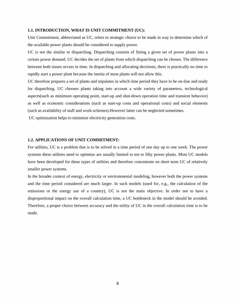
1.1. INTRODUCTION, WHAT IS UNIT COMMITMENT (UC):

Unit Commitment, abbreviated as UC, refers to strategic choice to be made in way to determine which of

the available power plants should be considered to supply power.

UC is not the similar to dispatching. Dispatching consists of fitting a given set of power plants into a

certain power demand. UC decides the set of plants from which dispatching can be chosen. The difference

between both issues occurs in time. In dispatching and allocating decisions, there is practically no time to

rapidly start a power plant because the inertia of most plants will not allow this.

UC therefore prepares a set of plants and stipulates in which time period they have to be on-line and ready

for dispatching. UC chooses plants taking into account a wide variety of parameters, technological

aspects(such as minimum operating point, start-up and shut-down operation time and transient behavior)

as well as economic considerations (such as start-up costs and operational costs) and social elements

(such as availability of staff and work-schemes).However latter can be neglected sometimes.

UC optimization helps to minimize electricity generation costs.

1.2. APPLICATIONS OF UNIT COMMITMENT:

For utilities, UC is a problem that is to be solved in a time period of one day up to one week. The power

systems these utilities need to optimize are usually limited to ten to fifty power plants. Most UC models

have been developed for these types of utilities and therefore concentrate on short term UC of relatively

smaller power systems.

In the broader context of energy, electricity or environmental modeling, however both the power systems

and the time period considered are much larger. In such models (used for, e.g., the calculation of the

emissions or the energy use of a country), UC is not the main objective. In order not to have a

disproportional impact on the overall calculation time, a UC bottleneck in the model should be avoided.

Therefore, a proper choice between accuracy and the utility of UC in the overall calculation time is to be

made.

9

1.3 LITERATURE REVIEW:

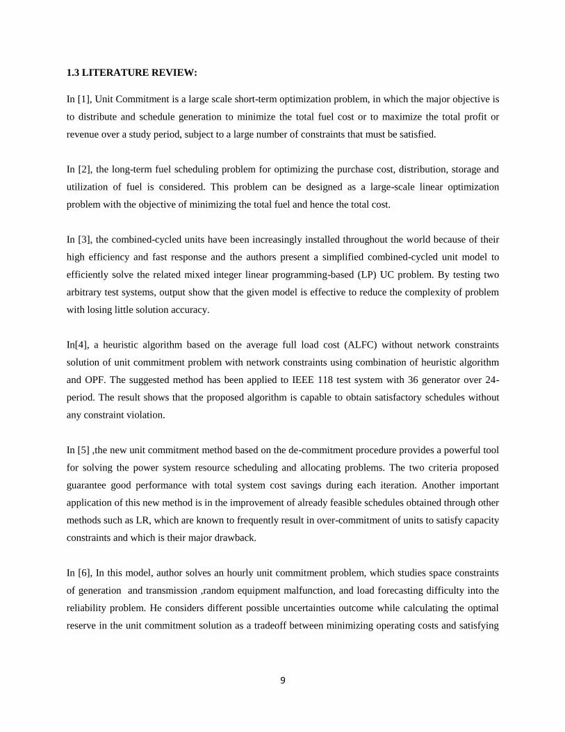
In [1], Unit Commitment is a large scale short-term optimization problem, in which the major objective is

to distribute and schedule generation to minimize the total fuel cost or to maximize the total profit or

revenue over a study period, subject to a large number of constraints that must be satisfied.

In [2], the long-term fuel scheduling problem for optimizing the purchase cost, distribution, storage and

utilization of fuel is considered. This problem can be designed as a large-scale linear optimization

problem with the objective of minimizing the total fuel and hence the total cost.

In [3], the combined-cycled units have been increasingly installed throughout the world because of their

high efficiency and fast response and the authors present a simplified combined-cycled unit model to

efficiently solve the related mixed integer linear programming-based (LP) UC problem. By testing two

arbitrary test systems, output show that the given model is effective to reduce the complexity of problem

with losing little solution accuracy.

In[4], a heuristic algorithm based on the average full load cost (ALFC) without network constraints

solution of unit commitment problem with network constraints using combination of heuristic algorithm

and OPF. The suggested method has been applied to IEEE 118 test system with 36 generator over 24-

period. The result shows that the proposed algorithm is capable to obtain satisfactory schedules without

any constraint violation.

In [5] ,the new unit commitment method based on the de-commitment procedure provides a powerful tool

for solving the power system resource scheduling and allocating problems. The two criteria proposed

guarantee good performance with total system cost savings during each iteration. Another important

application of this new method is in the improvement of already feasible schedules obtained through other

methods such as LR, which are known to frequently result in over-commitment of units to satisfy capacity

constraints and which is their major drawback.

In [6], In this model, author solves an hourly unit commitment problem, which studies space constraints

of generation and transmission ,random equipment malfunction, and load forecasting difficulty into the

reliability problem. He considers different possible uncertainties outcome while calculating the optimal

reserve in the unit commitment solution as a tradeoff between minimizing operating costs and satisfying

10

power system reliability requirements. Loss-of-load-expectation (LOLE) is included as a constraint in the

stochastic unit commitment for calculating the cost of supplying the reserve.

In [7], the EPL method consists of two stages; in the first stage we get any initial unit commitment

problem schedules by Priority List (PL) method. At this step, operational constraints are not taken into

account. In the second stage unit schedule is changed using the problem specific heuristics to fulfill

operational constraints.

In [8], the work done in this paper by using the forward dispatching, allocation modification and

backward dispatching, a generation allocation which satisfies the spinning reserve requirement and the

ramp rate limits are obtained. This schedule is automated by the future probabilistic reserve assessment to

meet a given risk value. The optimum value of this risk index is selected based on the tradeoff between

the total unit- commitment schedule cost and the expected cost of energy not served. Finally, a unit de-

commitment technique is incorporated to solve the problem of reserve over-commitment in Lagrangian

relaxation based unit commitment.

In [9] , Two-stage robust optimization formulation to address unit commitment problem in unit outages.

The overall problem is solved by using two-level cutting-plane algorithm, which converges within

reasonable time. The total cost under worst contingency over a selected uncertainty set is to be

minimized, so the resultant decisions have good robust performance if the uncertainty set is appropriately

defined. Besides the conventional (n – K) criterion, this paper provides a novel α-cut criterion that make

use of the information of probability distributions to reduce the operating cost.

In [10], Load forecasting accuracy has significant impact to the cost saving of all utilities in the planning

of energy supply. According to the recorded performance of Artificial Neural Network Short-term Load

forecaster being utilized in a real operational environment, the temperature forecast error is observed to be

the major cause of load forecast error. This paper describes the steps to develop an artificial neural

network model (ANN) for short term load forecast and proposed the enhancement of STLF engine by the

integration of front-end weather forecast model.

In [11], the multi-pass dynamic programming technique for the solution of the unit commitment and

hydrothermal generation scheduling problem. The problem formulation is very complicated and is more

complete than hydrothermal coordination. The algorithm is tested on Tai-power system with seven hydro

11

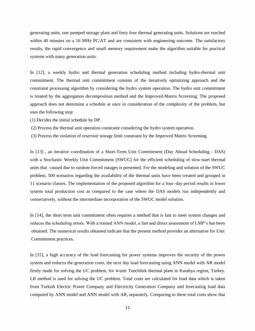
generating units, one pumped storage plant and forty four thermal generating units. Solutions are reached

within 40 minutes on a 16 MHz PC/AT and are consistent with engineering outcome. The satisfactory

results, the rapid convergence and small memory requirement make the algorithm suitable for practical

systems with many generation units.

In [12], a weekly hydro and thermal generation scheduling method including hydro-thermal unit

commitment. The thermal unit commitment consists of the iteratively optimizing approach and the

constraint processing algorithm by considering the hydro system operation. The hydro unit commitment

is treated by the aggregation decomposition method and the Improved-Matrix Screening. The proposed

approach does not determine a schedule at once in consideration of the complexity of the problem, but

uses the following step:

(1) Decides the initial schedule by DP.

(2) Process the thermal unit operation constraint considering the hydro system operation.

(3) Process the violation of reservoir storage limit constraint by the Improved Matrix Screening.

In [13] , an iterative coordination of a Short-Term Unit Commitment (Day Ahead Scheduling - DAS)

with a Stochastic Weekly Unit Commitment (SWUC) for the efficient scheduling of slow-start thermal

units that caused due to random forced outages is presented. For the modeling and solution of the SWUC

problem, 500 scenarios regarding the availability of the thermal units have been created and grouped in

11 scenario classes. The implementation of the proposed algorithm for a four–day period results in lower

system total production cost as compared to the case where the DAS models run independently and

consecutively, without the intermediate incorporation of the SWUC model solution.

In [14], the short term unit commitment often requires a method that is fast to meet system changes and

reduces the scheduling errors. With a trained ANN model, a fast and direct assessment of LMP‟s has been

obtained. The numerical results obtained indicate that the present method provides an alternative for Unit

Commitment practices.

In [15], a high accuracy of the load forecasting for power systems improves the security of the power

system and reduces the generation costs, the next day load forecasting using ANN model with AR model

firstly made for solving the UC problem, for 4-unit Tuncbilek thermal plant in Kutahya region, Turkey.

LR method is used for solving the UC problem. Total costs are calculated for load data which is taken

from Turkish Electric Power Company and Electricity Generation Company and forecasting load data

computed by ANN model and ANN model with AR, separately. Comparing to these total costs show that

12

load forecasting is important for UC. Furthermore, it is clear that the UC solution with the forecasting

load is better than without one in terms of total cost.

In [16] ,a large scale Unit Commitment (UC) problem has been solved using Conventional dynamic

programming (CDP), Sequential dynamic programming (SDP) and Truncation dynamic programming

(TDP) without time constraints and the results show the comparison of production cost and CPU time.

The UC provides a path to reduce the cost and improve reliability of the system. The Unit Commitment is

a dynamic process, and the generating strategy is always changing according to different load and

network topology.

13

CHAPTER2

ECONOMICS OF POWER GENERATION

14

2.1 ECONOMICS OF THE POWER GENERATION:

The function of a power station is to deliver power at the lowest possible cost per kilo watt hour. This

total cost is made up of fixed charges consisting of interest on the capital, taxes, insurance, depreciation

and salary of managerial staff, the operating expenses such as cost of fuels, water, oil, labor, repairs and

maintenance etc. The cost of power generation can be minimized by:

1. Choosing equipment that is available for operation during the largest possible % of time in a year.

2. Reducing the amount of investment in the plant.

3. Operation through fewer men.

4. Having uniform design

5. Selecting the station as to reduce cost of fuel, labor, etc.

All the electrical energy generated in a power station must be consumed

immediately as it cannot be stored. So the electrical energy generated in a power station must be regulated

according to the demand. The demand of electrical energy or load will also vary with the time and a

power station must be capable of meeting the maximum load at any time. Certain definitions related to

power station practice are given below:

Load curve: Load curve is plot of load in kilowatts versus time usually for a day or a year.

Load duration curve: Load duration curve is the plot of load in kilowatts versus time duration for which it

occurs.

Maximum demand: Maximum demand is the greatest of all demands which have occurred during a given

period of time.

Average load: Average load is the average load on the power station in a given period (day/month or

year)

Base load: Base load is the minimum load over a given period of time

Peak load: Peak load is the maximum load consumed or produced by a unit or group of units in a stated

period of time. It may be the maximum instantaneous load or the maximum average load over a

designated interval of time.

15

2.2 THERMAL GENERATION:

Thermal units provide a well-coordinated generation schedule to meet the power demand in the most

optimized effective and economical way. Generally the generation from thermal units is kept constant at

some particular base value and generation from different hydro units is varied according to the load

fluctuations as it is more easy to control hydro power and higher response rate then thermal generating

units.

Objective function

Thermal coordination is to find the optimal generating schedule of each unit so that the total system

production cost is minimum over the time range under schedule. Therefore the objective functions can be

expressed as follows:

Minimize ∑ ∑ ( )

………………….. (2.1)

Where

: the total system production cost

:number of hours at the time interval

: the cost function of thermal unit

the genration output of the ith thermal unit at the time stage

:the number of thermal units committed at the time interval

:maximum number of time stages

The cost functions of thermal generation units are expressed as second order polynomial.

……………………………………………….(2.2)

, and are constants.

16

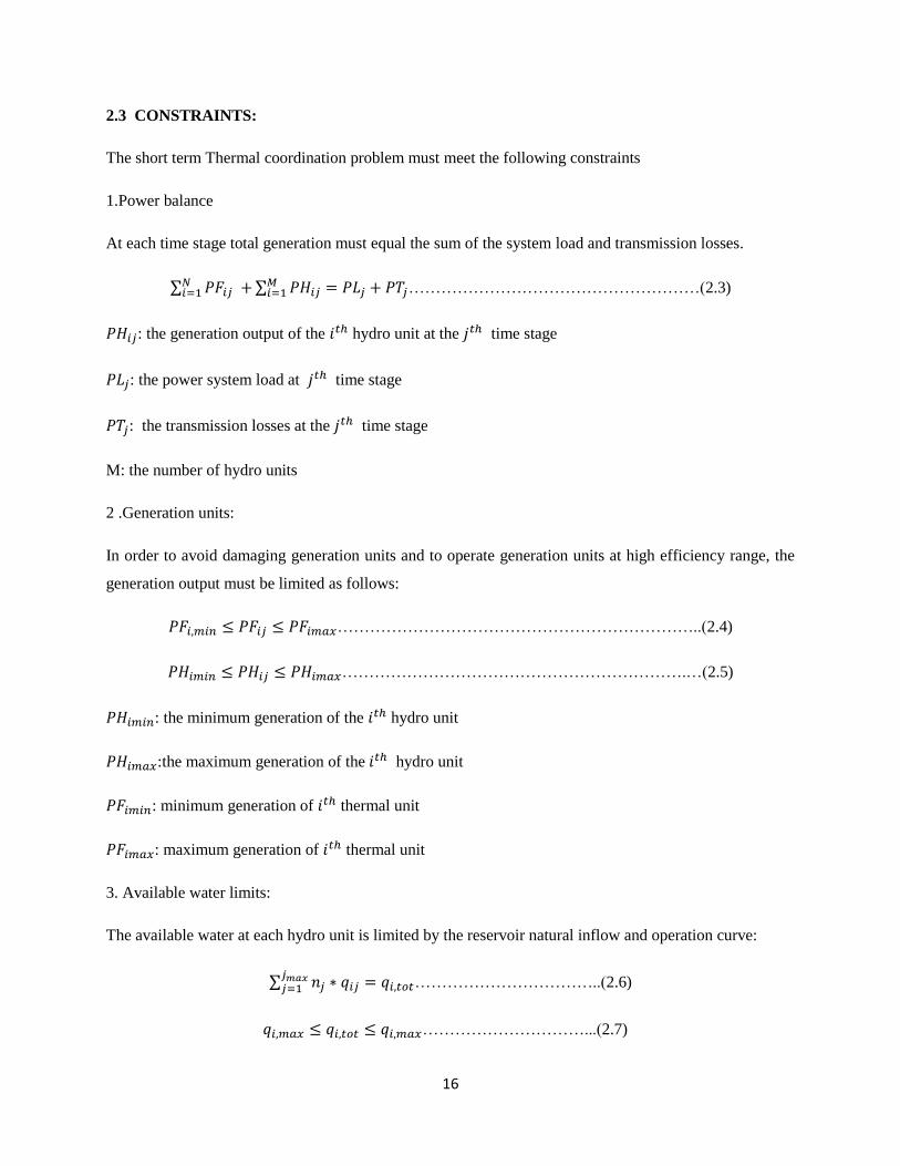
2.3 CONSTRAINTS:

The short term Thermal coordination problem must meet the following constraints

1.Power balance

At each time stage total generation must equal the sum of the system load and transmission losses.

∑ ∑

………………………………………………(2.3)

: the generation output of the hydro unit at the time stage

: the power system load at time stage

: the transmission losses at the time stage

M: the number of hydro units

2 .Generation units:

In order to avoid damaging generation units and to operate generation units at high efficiency range, the

generation output must be limited as follows:

…………………………………………………………..(2.4)

……………………………………………………….…(2.5)

: the minimum generation of the hydro unit

:the maximum generation of the hydro unit

: minimum generation of thermal unit

: maximum generation of thermal unit

3. Available water limits:

The available water at each hydro unit is limited by the reservoir natural inflow and operation curve:

∑ ……………………………..(2.6)

…………………………...(2.7)

17

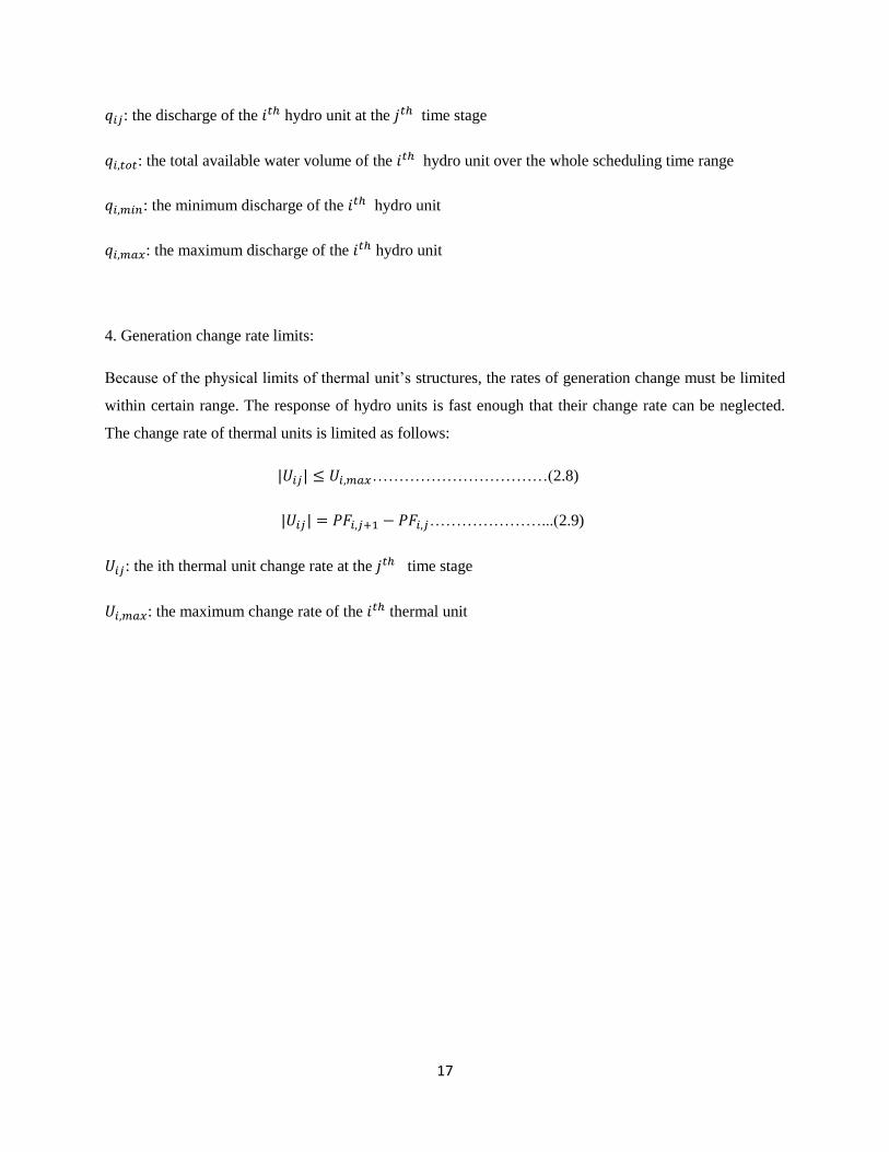
: the discharge of the hydro unit at the time stage

: the total available water volume of the hydro unit over the whole scheduling time range

: the minimum discharge of the hydro unit

: the maximum discharge of the hydro unit

4. Generation change rate limits:

Because of the physical limits of thermal unit‟s structures, the rates of generation change must be limited

within certain range. The response of hydro units is fast enough that their change rate can be neglected.

The change rate of thermal units is limited as follows:

……………………………(2.8)

…………………...(2.9)

: the ith thermal unit change rate at the time stage

: the maximum change rate of the thermal unit

18

CHAPTER3

METHODS OF UNIT COMMITMENT

19

3.1 METHOD OF EQUAL INCREMENTAL OF PRODUCTION COST :

3.1.1 INTRODUCTION: The economic load dispatch problem is defined as

∑ ………………………….. (3.1)

Subjected to = ∑ ………………..(3.2)

Where: : Total Fuel Input to the system.

: The fuel input to the unit.

: Total power demand.

: The generation from unit.

By making use of the Langrangian multiplier the auxiliary function is obtained as:

F = + λ ( - ∑ )………….(3.3)

Where: λ is the langrangian multiplier.

Differentiating F with respect to the generation and equating to zero gives the condition for optimal

operation of the system.

=

+ λ (0-1) = 0……………………,.(3.4)

=

– λ =0.

Since = + + ……. + …………..……..(3.5)

Therefore condition for optimum operation is

=

= …………….. =

= λ. …………………(3.6)

Where:

= incremental production cost of plant „n‟.

3.1.2 A MAJOR SETBACK TO THIS METHOD:

As we know, the fuel cost characteristic of any generating unit takes a differential form as follows :

20

F = A + (B*P) + (C* ). …………………………..(3.7)

≤ P ≤ . …………………………...……(3.8)

Where: F = total production cost.

P = total power generated from that unit.

A= Fixed production cost constant.

B, C = variable production cost constant.

= Maximum generation that can be obtained from that unit.

= Minimum generation from that unit.

Now as we know from the method of Equal Incremental of Production cost, for optimum production cost,

rate of generation from each unit in a system has to be same. When we differentiate the cost function and

equate that differentiated function to lambda „λ‟, we get the equation as follows:

B + (2 * C * P) = λ. ……………………………….(3.9)

Since every generating unit is associated with a Minimum and Maximum generation limit, there is also a

limit defined for the value of „λ‟ for each generating unit corresponding to ≤ λ ≤ .

Where : = B + (2*C* ) …………………………(3.10)

= B + (2*C* ) …………………………..(3.11)

Now for application of Method of Equal Incremental, each generating unit in a plant should have an

overlapping range of values of „lambda‟, which in most of the cases is not possible as any generating

plant consists of several unit having different generation limits. Any value of „lambda‟ not lying in the

specified range for that particular unit will lead to allocation of power which will be deviated from the

given range of power generation capability of that unit. So in all those cases it will be difficult to

implement this Method of Equal Incremental. This is one of the major setbacks of Equal Incremental

Production Cost method.

21

3.2 A MODIFIED APPOACH TO METHOD OF EQUAL INCREMENTAL:

3.2.1 INTRODUCTION: In this modified approach, we will be performing „n‟ no iterations for having the

final allotment of power through various generating units where „n‟ is the total no of generating units

involved for the Generation of that particular Demand.

In each iteration we will be calculating the value of „lambda‟ satisfying the total load demand for that

iteration. Corresponding to that „lambda‟ value, we will be calculating power allotted to each generating

unit.

= (λ – B ) / (2 * C); ……………………………….(3.12)

∑ = Demand. ………………………………….(3.13)

This first iteration is exactly same as that of the Method of Equal Incremental of Production Cost. Now

knowing the power allotted to different generating units, we will be calculating the total cost incurred

from each generating unit corresponding to their respective cost functions.

Suppose at the end of First iteration,

let power allotted to different units be , , ……… , .

and corresponding cost be , , …………, .

Since our main aim is to minimize the total cost of production, from the various cost ( , ,……, )

that we obtained, we will consider the unit having the minimum cost. [Minimum ( , ,……, ) ]. Let

that be any unit. For that unit we will see what was the power allotted initially ( ). If this power is

within the limits of generation of that unit, than we will fix the generation from that unit at . Now

for the next iteration, number of units will be (n-1) and total demand will be (Demand - ).

However, if does not fall in the specified range of power generation, than following alteration will be

made to the value of .

If > : ( which means for most economical production, generation from that unit should be

maximum ) : so in this case, we will set = . So for next iteration,

New Demand = Initial Demand-

22

If < : ( which means for most economical production, Generation from that unit should be

minimum ) : so in this case, we will set = 0. So for next iteration,

New Demand = Initial Demand.

After the first iteration is over, we will perform the other iterations in the same way as before but with

new Demand and reduced no of Generating units.

Iterations will continue till each generating unit has been assigned a particular power demand.

3.2.2 ADVANTAGE OF THIS METHOD:

With this new modified approach whatever be the size of the plant, whatever be the no of generating units

and whatever be the range of power generation of each unit, we can easily find the most optimized way to

allocate power among all the units with all the allocated power lying in the specified range for each

generating unit.

Problem of over-exhausting any unit by producing more than its specified level and also problem of

under-production from any unit is eliminated by this method as both the above circumstances not only

leads to more losses but also leads to continuous deterioration of generating units.

3.2.3 DRAWBACK OF THIS METHOD:

If we are considering for a station with large number of generating units, than for allocation of power to

each unit, number of iterations required will be more. For „n‟ number of units we will be performing „n‟

no iteration with each iteration consisting of finding suitable „lambda‟ satisfying the total demand for that

iteration. Since finding value of „lambda‟ itself is too time consuming task, the total time required for the

final allocation of power will be very large as compared to that of Original Equal Incremental Production

Cost Method.

Also, while calculating the value of „lambda‟, we always consider a particular deviation from the actual

demand i.e. total demand associated with any particular „lambda‟ value will deviate from original demand

by small amount ( ± some % of actual Demand ). Since in this method, in each iteration we are

calculating new value of „lambda‟, the total variation in the power Generated to that of the total Demand

is found to be somewhat more than that with Original Equal Incremental Production Cost Method.

23

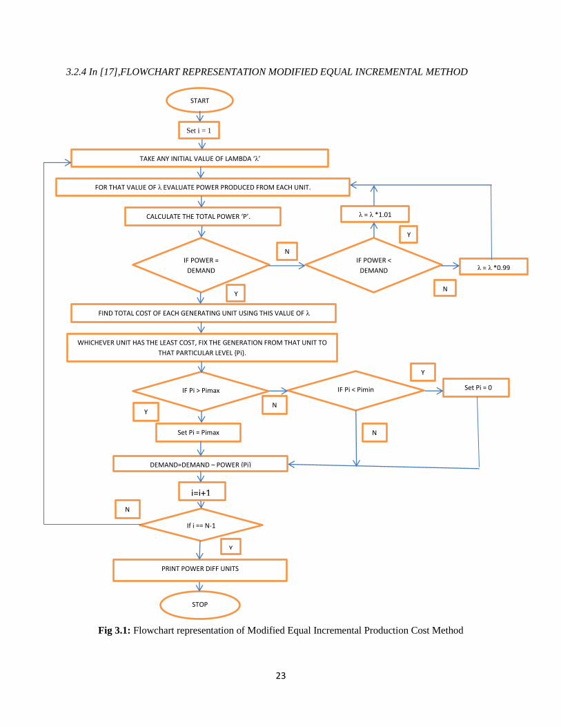
3.2.4 In [17],FLOWCHART REPRESENTATION MODIFIED EQUAL INCREMENTAL METHOD

Fig 3.1: Flowchart representation of Modified Equal Incremental Production Cost Method

TAKE ANY INITIAL VALUE OF LAMBDA ‘λ’

FOR THAT VALUE OF λ EVALUATE POWER PRODUCED FROM EACH UNIT.

CALCULATE THE TOTAL POWER ‘P’.

IF POWER =

DEMAND

IF POWER <

DEMAND

λ = λ *1.01

λ = λ *0.99

FIND TOTAL COST OF EACH GENERATING UNIT USING THIS VALUE OF λ

WHICHEVER UNIT HAS THE LEAST COST, FIX THE GENERATION FROM THAT UNIT TO

THAT PARTICULAR LEVEL {Pi}.

DEMAND=DEMAND – POWER {Pi}

If i == N-1

STOP

N

Y

Y

N

N

Y

START

IF Pi > Pimax

Set Pi = Pimax

IF Pi < Pimin Set Pi = 0

Set i = 1

i=i+1

PRINT POWER DIFF UNITS

YN

Y

N

24

3.3 LAMDA ‘λ’ ITERATIVE METHOD:

3.3.1 HIT AND TRIAL METHOD: In this Method, we will initially take any value of lambda. For that

value of „lambda‟ we will calculate power from each of the generating unit.

= (λ – B ) / (2 * C); ……………………………………(3.14)

Let P = ∑ . ………………………………………………(3.15)

For any Total Demand “D” -

if P>D – than we will decrease the value of „lambda‟ by .99 i.e. λ = λ*0.99.

if P<D – than we will increase the value of „lambda‟ by 1.01 i.e. λ = λ *1.01.

Than with this new value of „lambda‟, we will again calculate the total power and repeat the above steps

till we get a definite value of λ satisfying the load demand.

3.3.2 REGULAR FALSI-METHOD: In this method, we will take two initial values of „lambda‟

( . For both these values of „lambda‟ we will calculate total power from each of the units as

above –

= (λ – B ) / (2 * C);

Let P = ∑ .

For any load demand „D‟, we define error „e‟ as e = ( D – P ).

The initial values of „lambda‟ should be chosen such that for one „lambda‟ value we will get a positive

(+ve) error ( and for the other we get a negative (-ve) error ( ). This clearly means that desired value

of „lambda‟ lies between these two limits. For getting the desired value of „lambda‟, we will apply the

formula for regula-falsi method i.e.

25

λ = ( (

. …………….………..(3.16)

Now for this value of „lambda‟, we will calculate power from each unit and hence the total power ( ).

Than we will calculate the error ( ).

If > 0 i.e. (+ve), than

If < 0 i.e. (-ve), than .

With this new values of ( we will again calculate the total power and again new value of

„lambda‟ till we don`t get a that value of „lambda‟ for which error is zero or within certain acceptable

limit.

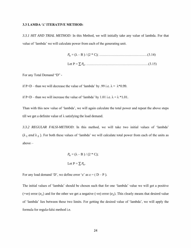
Fig 3.2 : Lambda iteration by Regula-Falsi Method

and corresponds to the two initial approximated values of Lambda such that error for 1 is positive

and other is negative and from the two values we are estimating the real value of Lambda

λ

λ

𝑒

𝑒 λ

26

3.4 PRIORITY LIST APPROACH FOR ECONOMIC LOAD DISPATCH:

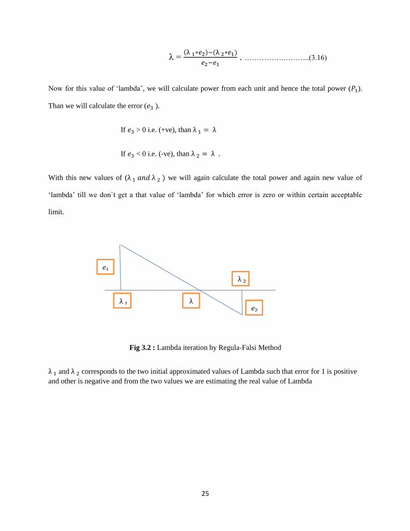
3.4.1 INTRODUCTON: This method is considered to be one of the simplest method of unit commitment

scheduling. This method consists of creating a priority list of all the generating units based on their

Average Full Load Cost (AFLC) value. Unit with the least value of AFLC is assigned the top most

priority and the rest according to the increasing value of AFLC.

This method is primarily based on the principle that unit with the least value of AFLC should be loaded to

the maximum level and the unit with the least value should be lightly loaded as this may fetch more

economical unit commitment solution.

The value of AFLC is calculated as follows :

= ( (

………………..(3.17)

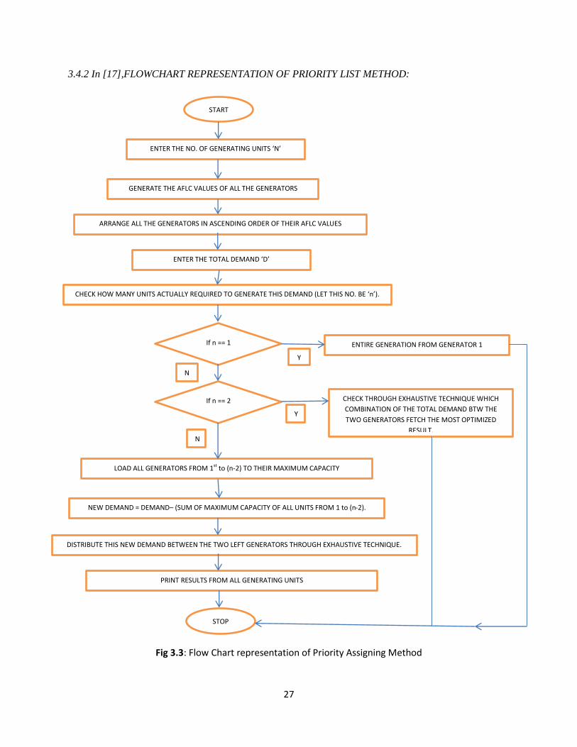
Following steps are followed for having unit commitment through Priority List Method –

- According to the AFLC value, arrange each generator in increasing order of their AFLC values.

Generator with least value is given the highest priority.

- Now according to the total demand „D‟, select how many generators required to fetch the given

demand i.e. ∑ of how many generators from top are giving the required Demand.

- If number „n‟ comes out to be one, than entire generation from that priority 1 unit.

- If „n‟ comes out to be two, than through exhaustive technique checking which combination of

power distribution between the two units is fetching the most optimized result.

- If „n‟ is coming greater than two, than all the generators from 1 to (n-2) will be loaded to their full

capacity. The power left after loading these (n-2) generators will be distributed between the two

left generators and through exhaustive technique, we will find the most optimized way to

distribute the remaining power between these two units.

27

3.4.2 In [17],FLOWCHART REPRESENTATION OF PRIORITY LIST METHOD:

Fig 3.3: Flow Chart representation of Priority Assigning Method

START

ENTER THE NO. OF GENERATING UNITS ‘N’

If n == 1

GENERATE THE AFLC VALUES OF ALL THE GENERATORS

ARRANGE ALL THE GENERATORS IN ASCENDING ORDER OF THEIR AFLC VALUES

ENTER THE TOTAL DEMAND ‘D’

CHECK HOW MANY UNITS ACTUALLY REQUIRED TO GENERATE THIS DEMAND (LET THIS NO. BE ‘n’).

If n == 2

ENTIRE GENERATION FROM GENERATOR 1

CHECK THROUGH EXHAUSTIVE TECHNIQUE WHICH

COMBINATION OF THE TOTAL DEMAND BTW THE

TWO GENERATORS FETCH THE MOST OPTIMIZED

RESULT.

LOAD ALL GENERATORS FROM 1st to (n-2) TO THEIR MAXIMUM CAPACITY

NEW DEMAND = DEMAND– (SUM OF MAXIMUM CAPACITY OF ALL UNITS FROM 1 to (n-2).

DISTRIBUTE THIS NEW DEMAND BETWEEN THE TWO LEFT GENERATORS THROUGH EXHAUSTIVE TECHNIQUE.

PRINT RESULTS FROM ALL GENERATING UNITS

STOP

N

Y

Y

N

28

CHAPTER4

RESULTS AND DISCUSSIONS

29

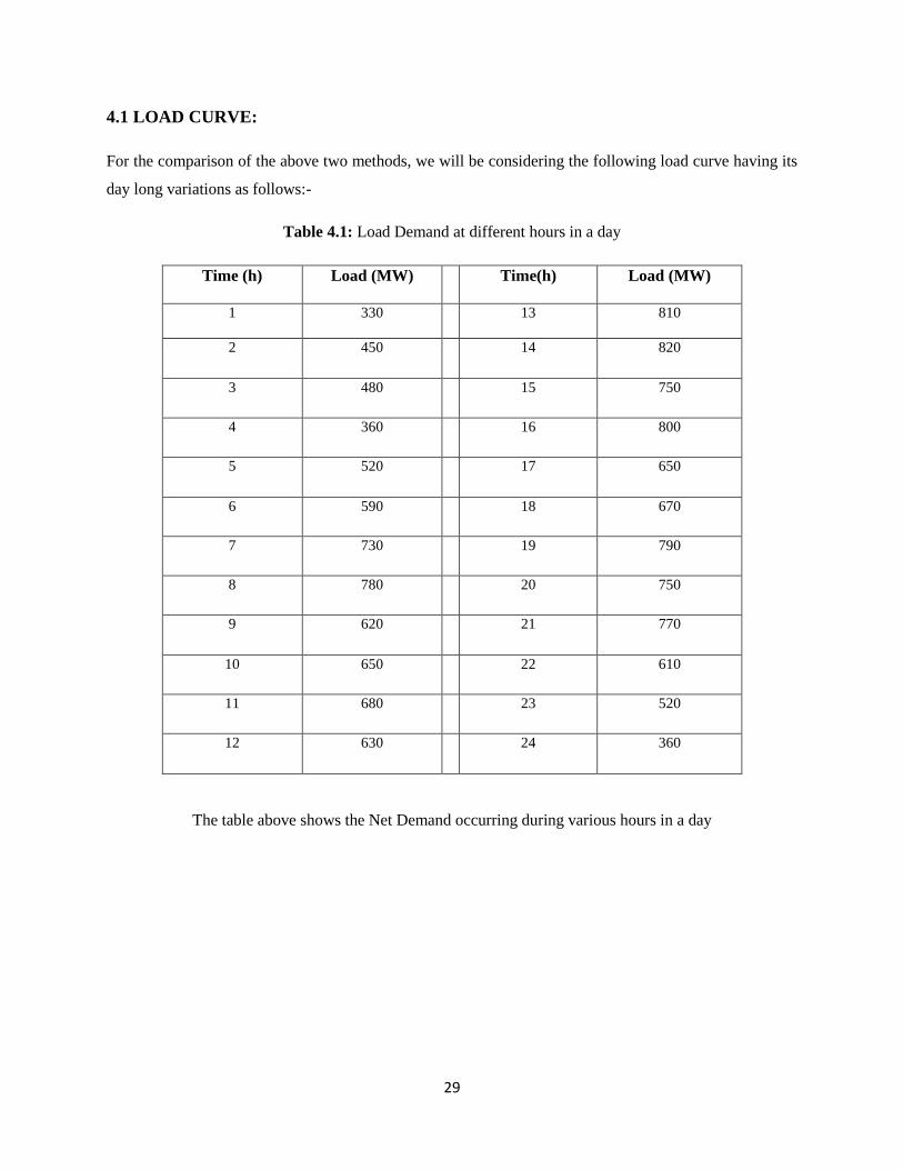
4.1 LOAD CURVE:

For the comparison of the above two methods, we will be considering the following load curve having its

day long variations as follows:-

Table 4.1: Load Demand at different hours in a day

Time (h) Load (MW) Time(h) Load (MW)

1 330 13 810

2 450 14 820

3 480 15 750

4 360 16 800

5 520 17 650

6 590 18 670

7 730 19 790

8 780 20 750

9 620 21 770

10 650 22 610

11 680 23 520

12 630 24 360

The table above shows the Net Demand occurring during various hours in a day

30

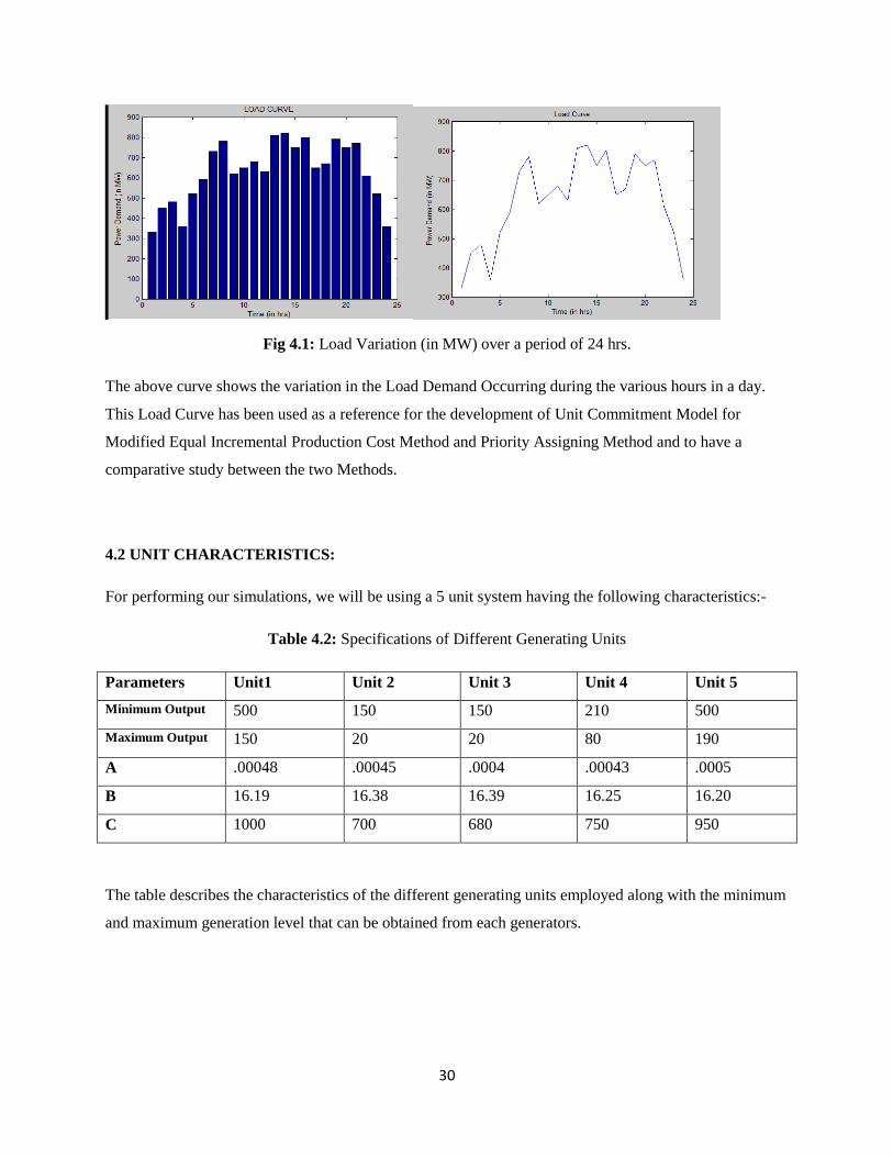
Fig 4.1: Load Variation (in MW) over a period of 24 hrs.

The above curve shows the variation in the Load Demand Occurring during the various hours in a day.

This Load Curve has been used as a reference for the development of Unit Commitment Model for

Modified Equal Incremental Production Cost Method and Priority Assigning Method and to have a

comparative study between the two Methods.

4.2 UNIT CHARACTERISTICS:

For performing our simulations, we will be using a 5 unit system having the following characteristics:-

Table 4.2: Specifications of Different Generating Units

Parameters Unit1 Unit 2 Unit 3 Unit 4 Unit 5

Minimum Output 500 150 150 210 500

Maximum Output 150 20 20 80 190

A .00048 .00045 .0004 .00043 .0005

B 16.19 16.38 16.39 16.25 16.20

C 1000 700 680 750 950

The table describes the characteristics of the different generating units employed along with the minimum

and maximum generation level that can be obtained from each generators.

31

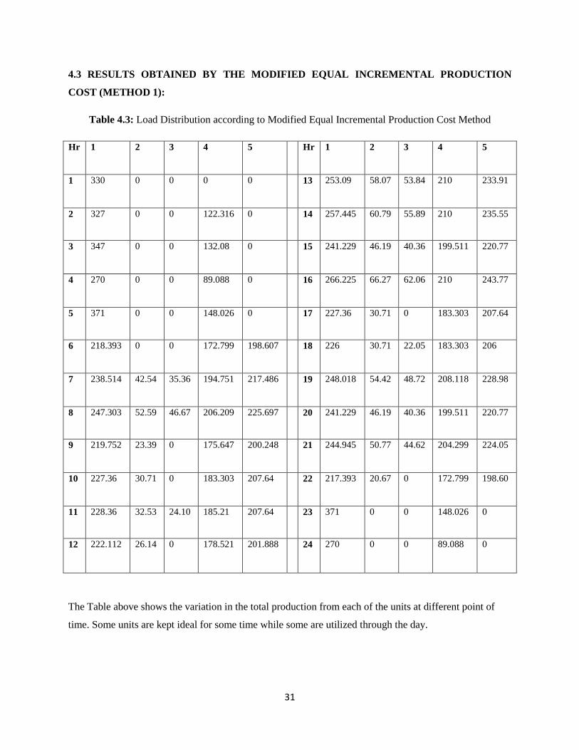
4.3 RESULTS OBTAINED BY THE MODIFIED EQUAL INCREMENTAL PRODUCTION

COST (METHOD 1):

Table 4.3: Load Distribution according to Modified Equal Incremental Production Cost Method

Hr 1 2 3 4 5 Hr 1 2 3 4 5

1 330 0 0 0 0 13 253.09 58.07 53.84 210 233.91

2 327 0 0 122.316 0 14 257.445 60.79 55.89 210 235.55

3 347 0 0 132.08 0 15 241.229 46.19 40.36 199.511 220.77

4 270 0 0 89.088 0 16 266.225 66.27 62.06 210 243.77

5 371 0 0 148.026 0 17 227.36 30.71 0 183.303 207.64

6 218.393 0 0 172.799 198.607 18 226 30.71 22.05 183.303 206

7 238.514 42.54 35.36 194.751 217.486 19 248.018 54.42 48.72 208.118 228.98

8 247.303 52.59 46.67 206.209 225.697 20 241.229 46.19 40.36 199.511 220.77

9 219.752 23.39 0 175.647 200.248 21 244.945 50.77 44.62 204.299 224.05

10 227.36 30.71 0 183.303 207.64 22 217.393 20.67 0 172.799 198.60

11 228.36 32.53 24.10 185.21 207.64 23 371 0 0 148.026 0

12 222.112 26.14 0 178.521 201.888 24 270 0 0 89.088 0

The Table above shows the variation in the total production from each of the units at different point of

time. Some units are kept ideal for some time while some are utilized through the day.

32

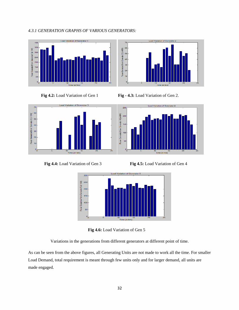
4.3.1 GENERATION GRAPHS OF VARIOUS GENERATORS:

Fig 4.2: Load Variation of Gen 1 Fig - 4.3: Load Variation of Gen 2.

Fig 4.4: Load Variation of Gen 3 Fig 4.5: Load Variation of Gen 4

Fig 4.6: Load Variation of Gen 5

Variations in the generations from different generators at different point of time.

As can be seen from the above figures, all Generating Units are not made to work all the time. For smaller

Load Demand, total requirement is meant through few units only and for larger demand, all units are

made engaged.

33

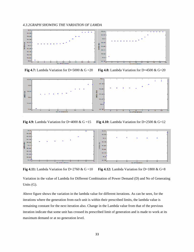
4.3.2GRAPH SHOWING THE VARIATION OF LAMDA

Fig 4.7: Lambda Variation for D=5000 & G =20 Fig 4.8: Lambda Variation for D=4500 & G=20

F



Variation in the value of Lambda for Different Combination of Power Demand (D) and No of Generating

Units (G).

Above figure shows the variation in the lambda value for different iterations. As can be seen, for the

iterations where the generation from each unit is within their prescribed limits, the lambda value is

remaining constant for the next iteration also. Change in the Lambda value from that of the previous

iteration indicate that some unit has crossed its prescribed limit of generation and is made to work at its

maximum demand or at no generation level.

34

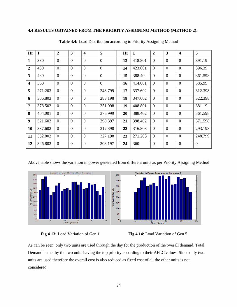
4.4 RESULTS OBTAINED FROM THE PRIORITY ASSIGNING METHOD (METHOD 2):

Table 4.4: Load Distribution according to Priority Assigning Method

Hr 1 2 3 4 5 Hr 1 2 3 4 5

1 330 0 0 0 0 13 418.801 0 0 0 391.19

2 450 0 0 0 0 14 423.601 0 0 0 396.39

3 480 0 0 0 0 15 388.402 0 0 0 361.598

4 360 0 0 0 0 16 414.001 0 0 0 385.99

5 271.203 0 0 0 248.799 17 337.602 0 0 0 312.398

6 306.803 0 0 0 283.198 18 347.602 0 0 0 322.398

7 378.502 0 0 0 351.998 19 408.801 0 0 0 381.19

8 404.001 0 0 0 375.999 20 388.402 0 0 0 361.598

9 321.603 0 0 0 298.397 21 398.402 0 0 0 371.598

10 337.602 0 0 0 312.398 22 316.803 0 0 0 293.198

11 352.802 0 0 0 327.198 23 271.203 0 0 0 248.799

12 326.803 0 0 0 303.197 24 360 0 0 0 0

Above table shows the variation in power generated from different units as per Priority Assigning Method

Fig 4.13: Load Variation of Gen 1 Fig 4.14: Load Variation of Gen 5

As can be seen, only two units are used through the day for the production of the overall demand. Total

Demand is met by the two units having the top priority according to their AFLC values. Since only two

units are used therefore the overall cost is also reduced as fixed cost of all the other units is not

considered.

35

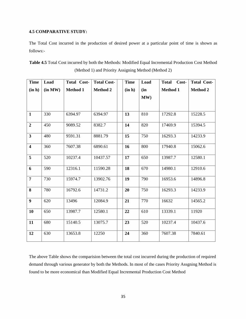
4.5 COMPARATIVE STUDY:

The Total Cost incurred in the production of desired power at a particular point of time is shown as

follows:-

Table 4.5 Total Cost incurred by both the Methods: Modified Equal Incremental Production Cost Method

(Method 1) and Priority Assigning Method (Method 2)

Time

(in h)

Load

(in MW)

Total Cost-

Method 1

Total Cost-

Method 2

Time

(in h)

Load

(in

MW)

Total Cost-

Method 1

Total Cost-

Method 2

1 330 6394.97 6394.97 13 810 17292.8 15228.5

2 450 9089.52 8382.7 14 820 17469.9 15394.5

3 480 9591.31 8881.79 15 750 16293.3 14233.9

4 360 7607.38 6890.61 16 800 17940.8 15062.6

5 520 10237.4 10437.57 17 650 13987.7 12580.1

6 590 12316.1 11590.28 18 670 14980.1 12910.6

7 730 15974.7 13902.76 19 790 16953.6 14896.8

8 780 16792.6 14731.2 20 750 16293.3 14233.9

9 620 13496 12084.9 21 770 16632 14565.2

10 650 13987.7 12580.1 22 610 13339.1 11920

11 680 15140.5 13075.7 23 520 10237.4 10437.6

12 630 13653.8 12250 24 360 7607.38 7840.61

The above Table shows the comparision between the total cost incurred during the production of required

demand through various generator by both the Methods. In most of the cases Priority Assgning Method is

found to be more economical than Modified Equal Incremental Production Cost Method

36

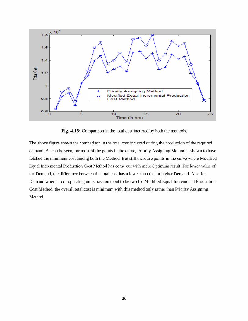
Fig. 4.15: Comparison in the total cost incurred by both the methods.

The above figure shows the comparison in the total cost incurred during the production of the required

demand. As can be seen, for most of the points in the curve, Priority Assigning Method is shown to have

fetched the minimum cost among both the Method. But still there are points in the curve where Modified

Equal Incremental Production Cost Method has come out with more Optimum result. For lower value of

the Demand, the difference between the total cost has a lower than that at higher Demand. Also for

Demand where no of operating units has come out to be two for Modified Equal Incremental Production

Cost Method, the overall total cost is minimum with this method only rather than Priority Assigning

Method.

37

CHAPTER5

CONCLUSIONS

38

5.1 CONCLUSIONS

- Total Cost incurred during the generation of the required demand was obtained for both the

methods i.e. Modified Equal Incremental Production Cost Method and Priority Assigning

Method.

- For maximum cases of power requirement, Priority Assigning Method was found to give more

optimized result in term of Total Cost than Modified Equal Incremental Production Cost Method.

- However, for certain cases, involving low power demand, Modified Equal Incremental

Production Cost Method were found to be better than Priority Assigning Method.

- Number of Units Operating for fulfilling a specific Load Demand was found to be more in case of

Modified Equal Incremental Production Cost Method.

- Since the no. of units are coming to be more, so the Fixed Cost of all the generating units adds up

to give an overall more Total Cost for Modified Equal Incremental Production Cost Method than

Priority Method.

- Variations in the value of Lambda for different iterations were obtained and were found to vary

considerably between successive iterations.

39

REFERENCES

1. D Srinivasan, senior member IEEE, J Chazelas,”A priority list-based evolutionary algorithm to solve

large scale unit commitment” 2004 International Conference on Power System Technology -

POWERCON 2004 Singapore, 21-24 November 2004.

2. G. E. Seymore, "Long-Term, Mid-Term, and Short-Term Fuel Scheduling", EPRI EL-2630, Volumes

1&2, Project 1048-6 Final Report, EPRI, Palo Alto, CA, January 1983.

3. G. W. Chang, M. Aganagic, J. G. Waight, J. Medina, T. Burton, S. Reeves, “Working with mixed

integer linear programming(LP) based approaches on short-term hydro scheduling units ,” IEEE

Transactions on Power Systems, Vol. 14, No. 3, Nov. 2001, pp. 742-749.

4. W.L. Snyde.Jr., H.DPowel1, J.C.Rayburn, “Dynamic Programming Approach to Unit Commitment”,

IEEE Trans. on Power Systems, Vol PERS-2, No.2, pp.339-350, 1987.

5. Chao-an Li, Raymond B. Johnson (Member, IEEE), Alva J. Svoboda (Member, IEEE),” A new unit

commitment method” IEEE Transactions on Power Systems, Vol. 13, No. 2, February 1996.

6. Lei Wu,Member, IEEE, Mohammad Shahidehpour, Fellow, IEEE, and Tao Li, Member, IEEE,” Cost

of Reliability Analysis Based on Stochastic Unit Commitment” IEEE transactions on power system,

VOL. 27, NO. 2, AUGUST 2008.

7. H. Mori and Matsuzaki, “ Application of Priority-List-Embedded Tabu Search to Unit Commitment in

Power Systems ” , IEEJ, Vol. 101-B, NO. 3, pp. 535-551, 2003.

8. A. Merlin and P. Sandrin, “A New Method for Unit Commitment at Electricity in France ”, lEEE

Transactions on Power Systems, Vol. PAS-102, No. 5, pp. 1218-1225, May 1983.

9. A. Street, F. Oliveira, and J. Arroyo, “A constrained unit commitment with n − k security criterion: A

robust optimization approach,” IEEE Trans. Power. Syst., vol. 28, no. 4, pp. 1581–1591,2011.

10. A.D. Papalexopoulos, T. C. Hesterberg, “A regressive approach to short-term load forecasting,” IEEE

Trans Power Syst., vol. 7, pp. 1537-1547, 1991.

40

11. Jin-Shyr Yang, Member IEEE Nanming Chen , Member, IEEE,” unit commitment and hydrothermal

generation scheduling by multi-pass dynamic programming” Proceedings of 29th Conference on Decilon

and Control Honolulu, December 1990.

12. S. Soares, C. Lya and H. Tavares, “Qptimal Generation Scheduling of Hydrothermal Power Systems",

IEEE Trans. PAS, Vol. PAS-97, No. 2, pp.l104-lIlS, MaylJune 1986.

13. Pandelis N. Biskas, Costas G. Baslis, Christos K. Simoglou, Anastasios G. Bakirtzis” Coordination of

Day-Ahead Scheduling with a Stochastic Weekly Unit Commitment for the efficient scheduling of slow-

start thermal units” 2010 IREP Symposium- Bulk Power System Dynamics and Control – VIII (IREP),

August 1-6, 2010, Buzios, RJ, Brazil.

14. W. L.Snyder, H. D. Powell and J. C. Raybum,” Dynamic Programming Approach to Unit

Commitment”, IEEE Trans. PWRS-2(2), pp.339- 350, 1987

15. Titti Saksornchai, Wei-Jen Lee, Member, IEEE,James R. Liao, Member, IEEE, and Richard J. Ross”

“Improve the Unit Commitment Scheduling by Using the Neural-Network-Based Short-Term Load

Forecasting” IEEE TRANSACTIONS ON INDUSTRY APPLICATIONS, VOL. 45, NO. 1,

JANUARY/FEBRUARY 2006

16. J. Muksadt, “The use of Mixed- Integer Programming Duality to Scheduling Thermal Generating

Systems,” IEEE Transactions on Power equipments and Systems, vol. PAS-87, no. 12, pp. 1968-1978,

December 1968

17. Joon-Hyung Park, Sun-Kyo Kim, “Modified Dynamic Programming Based Unit Commitment

Technique”, IEEE conference paper, 2010.

a comparative study between priority assigning method...

Documents