a comparative study between a small time scale model and the two driving force model for fatigue...

International Journal of Fatigue 42 (2012) 57–70

Contents lists available at ScienceDirect

International Journal of Fatigue

journal homepage: www.elsevier .com/locate / i j fa t igue

A comparative study between a small time scale model and the twodriving force model for fatigue analysis

Zizi Lu, Yongming Liu ⇑Clarkson University, Potsdam, NY 13699, USA

a r t i c l e i n f o

Article history:Received 29 September 2010Received in revised form 28 April 2011Accepted 18 May 2011Available online 27 May 2011

Keywords:Two driving force approachSmall time scaleFatigue crack growth

0142-1123/$ - see front matter � 2011 Elsevier Ltd. Adoi:10.1016/j.ijfatigue.2011.05.016

⇑ Corresponding author. Tel.: +1 315 268 2341; faxE-mail address: [email protected] (Y. Liu).

a b s t r a c t

A comparative study is performed to demonstrate the difference and similarity between the two drivingforce approach and a small time scale model under both constant and variable amplitude loading. Thesmall time scale model is different from most existing fatigue analysis methodologies and is based onthe instantaneous crack growth kinetics within one cycle. The two driving force approach is cycle-basedand uses two driving force parameters to describe crack growth rate per cycle under constant amplitudeloadings. A simple modified two driving force approach is proposed based on the concept of forward andreverse plastic zone interaction and is used to calculate the fatigue crack growth under general variableamplitude loadings. Extensive experimental data for various metallic materials are used to validate thetwo driving force model and the small time scale model.

� 2011 Elsevier Ltd. All rights reserved.

1. Introduction

Most existing fatigue crack growth prediction models are cycle-based, in which the smallest time scale is one cycle. However, fati-gue damage accumulation process is a multi-scale phenomenon,which involves very different spatial and temporal scales. The cy-cle-based approach is not able to capture the detailed mechanismat the sub-cycle scale. A new fatigue crack growth formulation,i.e., small time scale model, based on the small time scale crackincrement instead of cycle-based approach is developed by thesame authors [1]. This method is based on the incremental crackgrowth at any time instant during one cycle. The forward and re-verse plastic zone interaction is used to explain the nonlinear crackgrowth kinetics within one loading cycle, in which the crack closurehypothesis is used to estimate the plastic zone size. The equivalentcycle-based formula of the small time scale model shows that twodriving force parameters (i.e., Kmax and DK) is required to describethe crack growth rate under constant amplitude loadings [1]. Thus,it will be helpful to evaluate the difference and similarities betweenthe widely used two driving force approach and the small time scaleformulation.

The two driving force (e.g., DK and Kmax) approach was firstlyintroduced by Sadananda and Vasudevan [2,3] in order to describecrack growth rates. Based on the two driving force concept, Kujaw-ski [4,5] proposed a two driving force fatigue crack growth modelby defining a new effective crack driving parameter consideringboth DK and Kmax terms.

ll rights reserved.

: +1 315 268 7985.

A two driving force model accounting for the variable amplitudeloading history effects, named UniGrow model was proposed in[6]. The UniGrow model is based on the analysis of the elastic–plastic strain–stress history near the crack tip. Although the Uni-Grow methodology is an attractive method for fatigue analysis un-der random variable amplitude loading, it requires a sophisticateddetermination of different loading and unloading regimes in crackgrowth simulation. In addition, this approach requires the discret-ization of crack tip zone into many small spring elements, which iscomputationally expensive for large structural applications.

The main objective of this study is to compare the two drivingforce approach with a previously developed small time scale modelfor fatigue crack growth prediction under both constant amplitudeloading and variable loading. A new and simple two driving forcemethodology is proposed for fatigue crack growth predictions un-der various variable amplitude loading histories. The coupling ef-fect under variable loading is included using the small time scalemechanism modeling. The advantage of the proposed approach isthat it has the simple form of the two driving force approach andis very efficient in handling the variable spectrum loadings. Exper-imental validation shows generally very good prediction accuracyfor the proposed approach. Some conclusions are drawn based onthe proposed study.

2. Model description

In this section, the small time scale model is briefly discussedfirst to show the basic concept and hypotheses. Following this,the widely used two driving force approach is discussed. A modi-fied version under variable amplitude loading is proposed, which

http://dx.doi.org/10.1016/j.ijfatigue.2011.05.016

mailto:[email protected]

http://dx.doi.org/10.1016/j.ijfatigue.2011.05.016

http://www.sciencedirect.com/science/journal/01421123

http://www.elsevier.com/locate/ijfatigue

Old crack surface

Current crack surface at t+dt

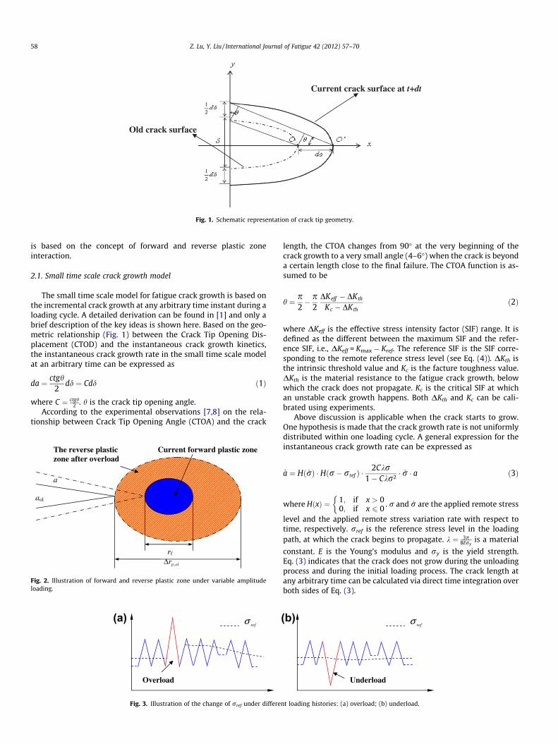
Fig. 1. Schematic representation of crack tip geometry.

58 Z. Lu, Y. Liu / International Journal of Fatigue 42 (2012) 57–70

is based on the concept of forward and reverse plastic zoneinteraction.

2.1. Small time scale crack growth model

The small time scale model for fatigue crack growth is based onthe incremental crack growth at any arbitrary time instant during aloading cycle. A detailed derivation can be found in [1] and only abrief description of the key ideas is shown here. Based on the geo-metric relationship (Fig. 1) between the Crack Tip Opening Dis-placement (CTOD) and the instantaneous crack growth kinetics,the instantaneous crack growth rate in the small time scale modelat an arbitrary time can be expressed as

da ¼ ctgh2

dd ¼ Cdd ð1Þ

where C ¼ ctgh2 . h is the crack tip opening angle.

According to the experimental observations [7,8] on the rela-tionship between Crack Tip Opening Angle (CTOA) and the crack

The reverse plastic zone after overload

Current forward plastic zone

rf

aol

a

olpr ,Δ

Fig. 2. Illustration of forward and reverse plastic zone under variable amplitudeloading.

Overload

refσ(a)

Fig. 3. Illustration of the change of rref under differe

length, the CTOA changes from 90� at the very beginning of thecrack growth to a very small angle (4–6�) when the crack is beyonda certain length close to the final failure. The CTOA function is as-sumed to be

h ¼ p2� p

2DKeff � DKth

Kc � DKthð2Þ

where DKeff is the effective stress intensity factor (SIF) range. It isdefined as the different between the maximum SIF and the refer-ence SIF, i.e., DKeff = Kmax � Kref. The reference SIF is the SIF corre-sponding to the remote reference stress level (see Eq. (4)). DKth isthe intrinsic threshold value and Kc is the facture toughness value.DKth is the material resistance to the fatigue crack growth, belowwhich the crack does not propagate. Kc is the critical SIF at whichan unstable crack growth happens. Both DKth and Kc can be cali-brated using experiments.

Above discussion is applicable when the crack starts to grow.One hypothesis is made that the crack growth rate is not uniformlydistributed within one loading cycle. A general expression for theinstantaneous crack growth rate can be expressed as

_a ¼ Hð _rÞ � Hðr� rref Þ �2Ckr

1� Ckr2 � _r � a ð3Þ

where HðxÞ ¼ 1; if x > 00; if x 6 0

�. r and _r are the applied remote stress

level and the applied remote stress variation rate with respect totime, respectively. rref is the reference stress level in the loadingpath, at which the crack begins to propagate. k ¼ 3p

8Eryis a material

constant. E is the Young’s modulus and ry is the yield strength.Eq. (3) indicates that the crack does not grow during the unloadingprocess and during the initial loading process. The crack length atany arbitrary time can be calculated via direct time integration overboth sides of Eq. (3).

Underload

refσ(b)

nt loading histories: (a) overload; (b) underload.

Table 1Summary of experimental data under constant amplitude loading.

Materials Yieldstrength ry (MPa)

Ultimatestrength ru (MPa)

Modulus ofelasticity E (MPa)

Stress ratio R Ref.

Al 2024-T3 360 490 72,000 �2, �1, �0.5, 0, 0.5, 0.7 [13]Al 7050-T7451 455 515 68,000 0.02, 0.1, 0.33, 0.5, 0.75 [13]Al 7075-T6 520 575 72,000 0.08, 0.1, 0.4, 0.5, 0.7, 0.8 [13]300M steel 1380 1770 205,000 0.05, 0.3, 0.5, 0.7 [14]4340 steel 1410 1510 72,000 �1, 0, 0.5, 0.7 [15]Ti–10V–2Fe–3Al 1028 1047 103,000 0.1, 0.5, 0.8 [16]

Table 2Summary of parameters for all materials.

Materials Thickness(mm)

DKth

(MPa m1/2)Kc

(MPa m1/2)C a p

Al 2024-T3 2.3 0.9 96 1.43e�11 0.511 3.54Al 7050-T7451 2.3 0.9 72.3 1.42e�11 0.469 3.60Al 7075-T6 2.3 0.8 36.5 1.21e�12 0.461 3.05300M steel 1.4 0.9 91 1.46e�11 0.272 2.844340 steel 5.1 0.8 198 3.45e�11 0.616 2.24Ti–10V–2Fe–3Al 8 0.8 116 5.80e�12 0.3524 3.34

100 110-9

10-8

10-7

10-6

10-5

10-4

Δ K (M

da/d

N (m

/cyc

le)

Al 7075-T6

100 101 10210-9

10-8

10-7

10-6

10-5

10-4 Two Driving Force Model

da/d

N (m

/cyc

le)

PredictionR= 0.02R= 0.1R= 0.33R= 0.5R= 0.75

Al 7075-T6

ΔKeq (MPa-m0.5)

(

(b)Fig. 4. Analysis of crack growth data for Al 7075-T6: (a) crack growth data of as a functiondriving force model, and (c) small time scale model.

Table 3Normalized Kref under constant amplitude loading history for Al 7075-T6.

R-ratio �1 �0.5 0.0 0.33 0.4 0.5 0.7

Kref �0.37 0.02 0.32 0.55 0.60 0.66 0.80

Z. Lu, Y. Liu / International Journal of Fatigue 42 (2012) 57–70 59

The classical crack growth rate per cycle (e.g., da/dN) can be ob-tained by the direct integration of Eq. (3) during one loading cycleas

01 102

Pa-m.5)

R= 0.02R= 0.1R= 0.33R= 0.5R= 0.75

100 101 10210-9

10-8

10-7

10-6

10-5

10-4Small Time Scale Model

da/d

N (m

/cyc

le)

PredictionR= 0.02R= 0.1R= 0.33R= 0.5R= 0.75

Al 7075-T6

ΔKeq (MPa-m0.5)

a)

(c)of DK; crack growth data of as a function of DKeq with the prediction curve, (b) two


Da ¼ dadN¼

pCka r2max � r2

ref

� �p 1� Ckr2

max

� � ¼Ck K2

max � K2ref

� �p 1� Ckr2

max

� � ð4Þ

It is shown in Eq. (4) that the equivalent cycle-based formula ofthe small time scale model includes two driving force parameters,which are consistent with the two driving force approach assump-tions. This is one of the motivations that we propose a comparativestudy between these two different approaches.

Above discussions are for constant amplitude loadings and theidea can be extended to variable amplitude loadings. The conceptof forward and reverse plastic zone interaction is used for the var-iable amplitude loading ‘‘memory’’ effect. Unlike the crack tip plas-ticity under monotonic loading, there are two plastic zones underfatigue cyclic loading: forward plastic zone during the loading pathand reverse plastic zone during the unloading path [9]. A schematicillustration of the proposed model is shown in Fig. 2. In Fig. 2, thereverse plastic zone is shown as the textured area and the forwardplastic zone is shown as the shaded area. The reverse plastic zoneafter the unloading produces compressive residual stress fieldsahead of the crack tip. Crack will not grow unless the compressiveresidual stress is reversed, which indicates that crack will onlygrow beyond a certain stress level rref in the loading path, i.e.,when the present forward plastic zone size reaches the previousreverse plastic zone size ahead of the crack tip [1].

Under constant amplitude loadings, the largest reverse plasticzone size at any time point always comes from the previous near-

100 10110-9

10-8

10-7

10-6

10-5

10-4

Δ K (MPa

da/d

N (m

/cyc

le)

Al 2024-T3

100 101 102 10310-9

10-8

10-7

10-6

10-5

10-4Two Driving Force Model

da/d

N (m

/cyc

le)

PredictionR= -1R= -0.5R= 0R= 0.33R= 0.4R= 0.5R= 0.7

Al 2024-T3

ΔKeq (MPa-m0.5)

(a)

(b)Fig. 5. Analysis of crack growth data for Al 2024-T3: (a) crack growth data of as a functiondriving force model, and (c) small time scale model.

est unloading process. However, as for the variable amplitude load-ing, the largest reverse plastic zone size may come from a previousunloading process far from the current time point (e.g., a largeoverload before the current loading cycle). The current forwardplastic zone has to go beyond the largest reverse plastic zone in or-der to grow the crack. As it is shown in Fig. 2, an overload is appliedwhen the crack length is aol and the resulted reverse plastic zone isDrp,ol. At the current calculation, the crack length is a and the cur-rent forward plastic zone size is rf. It is seen that the largest reverseplastic zone produced from a previous overload may affect thecrack growth many cycles after the overload. This is known asthe ‘‘memory effect’’ during the variable amplitude loading crackgrowth, such as the overload retardation.

In order to represent the mechanism in Fig. 2, a modified limitstate function is proposed to calculate the rref as

aol þ Drp;ol ¼ aþ rf ð5Þ

The left side of Eq. (5) calculates the coordinate of the largest re-verse plastic zone boundary and the right side of Eq. (5) calculatesthe coordinate of the current forward plastic zone boundary. Eq.(5) is also applicable to the constant loading case and is the generallimit state function in determining the reference stress level undervariable amplitude loading.

A schematic illustration for one constant loading history in-serted with an overload/underload is shown in Fig. 3. It is shownthat the rref (i.e., the lower integration stress level) is different

102

-m.5)

R= -1R= -0.5R= 0R= 0.33R= 0.4R= 0.5R= 0.7

10-1 100 101 10210-10

10-9

10-8

10-7

10-6

10-5

10-4 Small Time Scale Model

da/d

N (m

/cyc

le)

PredictionR= -1R= -0.5R= 0R= 0.33R= 0.4R= 0.5R= 0.7

Al 2024-T3

ΔKeq (MPa-m0.5)



due to the interaction of forward and reversed plastic zone,although the maximum stress levels are same. The rref increasesto a higher level after an overload inserted into the regular con-stant amplitude loading history as it shown in Fig. 3a and will re-duce to the regular level after a certain crack growth length.Overload retardation happens since the crack growth per cycle isreduced due to increased lower integration stress level. Similarly,the rref decreases following an underload and the underload accel-eration phenomenon happens.

One advantage of the proposed small time scale model is that itcan be used for fatigue analysis at variable time and length scales.The fatigue crack growth analysis under random variable ampli-tude loading can be performed without cycle-counting. Anotheradvantage is that the small time scale model includes the stress ra-tio effect intrinsically since the direct stress state instead of thestress range is used.

2.2. Two driving force approach

Since the comprehensive review and discussion of the two driv-ing force approach is not the focus of this study. Only a brief intro-duction is described here. Detailed derivations can be found in thereferred articles. Based on the two driving force concept, Kujawski[4] proposed a two driving force fatigue crack growth model bydefining a new effective crack driving parameter as

100 10110-10

10-9

10-8

10-7

10-6

10-5

Δ K (MP

da/d

N (m

/cyc

le)

Al 7050-T7451

100 101 10210-10

10-9

10-8

10-7

10-6


da/d

N (m

/cyc

le)

PredictionR= 0.08 R= 0.1R= 0.4R= 0.5 R= 0.7R= 0.8

Al 7050-T7451

ΔKeq (MPa-m0.5)

(a)

(b)Fig. 6. Analysis of crack growth data for Al 7050-T7451: (a) crack growth data of as a funtwo driving force model, and (c) small time scale model.

DK� ¼ ðKmax � DKþÞ0:5 ð6Þ

where DK+ is the positive part of the applied stress intensity factor(SIF) range, and Kmax is the corresponding maximum value of theapplied SIF. This model was then modified to be a more generalform [5] as

DK� ¼ DKð1�aÞ � Kamax ð7Þ

The data under various R-ratios can be consolidated to a singlemaster curve by incorporating the simple mathematical transfor-mation of the Paris equation. The two driving force model for fati-gue crack growth is expressed by replacing the DK in Paris lawwith the DK� as

da=dN ¼ C � ðDKð1�aÞ � KamaxÞ

p ð8Þ

Model validations in [5,10–12] suggested that the revised twodriving force model (Eq. (7)) works better for some engineeringmaterials compared to its original format (Eq. (6)). Therefore, theEq. (8) is used in this comparative study.

Above discussion is for the application of the two driving forceapproach under constant amplitude loadings. Compared to theextensive studies of the two driving force approaches under con-stant variable loading, very few studies focused on the extensionto the variable amplitude loading. The UniGrow [6] model is prob-ably the only one available in the open literature. The UniGrow

102

a-m.5)

R= 0.08R= 0.1R= 0.4R= 0.5R= 0.7R= 0.8

10-1 100 101 10210-10

10-9

10-8

10-7

10-6


da/d

N (m

/cyc

le)

PredictionR= 0.08 R= 0.1R= 0.4R= 0.5R= 0.7R= 0.8

Al 7050-T7451

ΔKeq (MPa-m0.5)

(c)ction of DK; crack growth data of as a function of DKeq with the prediction curve, (b)


model explains the overload retardation with the internal stressand requires a discretization of the crack tip region. The elementsize in the discretization zone needs calibration using experimen-tal data. The UniGrow model is an attractive model, but requiresdetailed analysis of crack tip stress/strain response. In this paper,a simple modified two driving force approach is proposed for var-iable amplitude loading cases. The comparison with the UniGrowmodel needs further investigation.

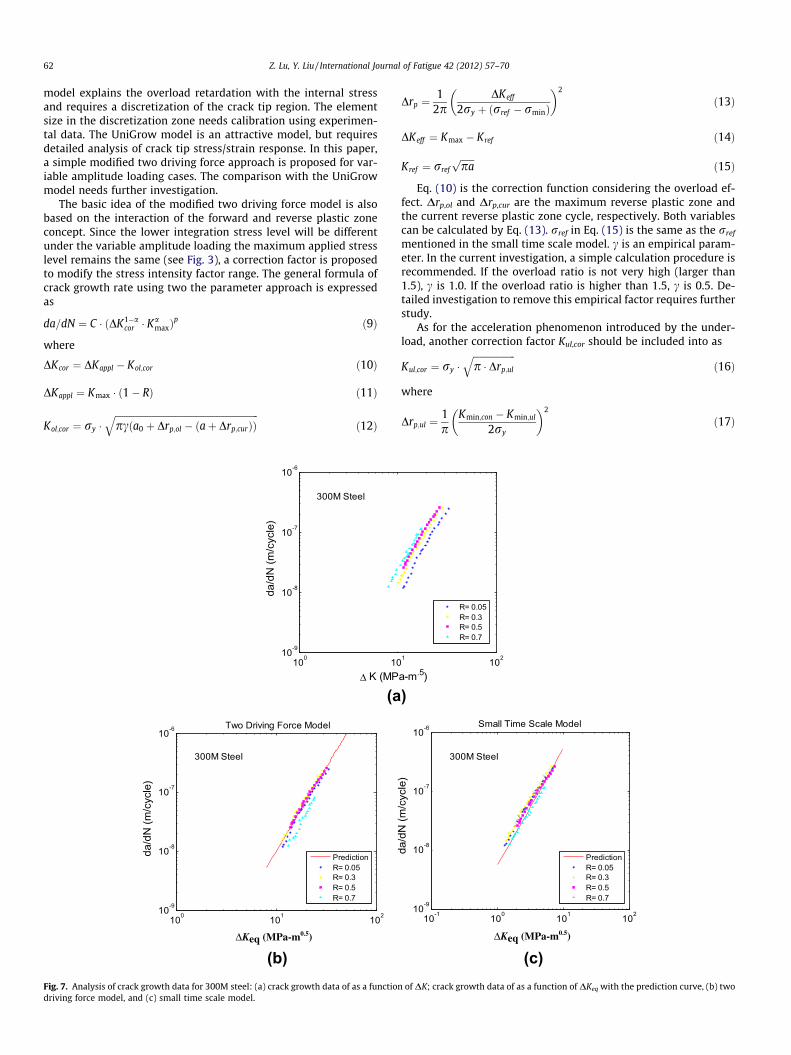
The basic idea of the modified two driving force model is alsobased on the interaction of the forward and reverse plastic zoneconcept. Since the lower integration stress level will be differentunder the variable amplitude loading the maximum applied stresslevel remains the same (see Fig. 3), a correction factor is proposedto modify the stress intensity factor range. The general formula ofcrack growth rate using two the parameter approach is expressedas

da=dN ¼ C � ðDK1�acor � K

amaxÞ

p ð9Þ

where

DKcor ¼ DKappl � Kol;cor ð10Þ

DKappl ¼ Kmax � ð1� RÞ ð11Þ

Kol;cor ¼ ry �ffiffiffiffiffiffiffiffiffiffiffiffiffiffiffiffiffiffiffiffiffiffiffiffiffiffiffiffiffiffiffiffiffiffiffiffiffiffiffiffiffiffiffiffiffiffiffiffiffiffiffiffiffiffiffiffiffiffiffiffiffiffipcða0 þ Drp;ol � ðaþ Drp;curÞÞ

qð12Þ

100 1010-9

10-8

10-7

10-6

Δ K (MP

da/d

N (m

/cyc

le)

300M Steel

100 101 10210-9

10-8

10-7


da/d

N (m

/cyc

le)

PredictionR= 0.05R= 0.3R= 0.5R= 0.7

300M Steel

ΔKeq (MPa-m0.5)

(a

(b)Fig. 7. Analysis of crack growth data for 300M steel: (a) crack growth data of as a functiondriving force model, and (c) small time scale model.

Drp ¼1

2pDKeff

2ry þ ðrref � rminÞ

� 2

ð13Þ

DKeff ¼ Kmax � Kref ð14Þ

Kref ¼ rref

ffiffiffiffiffiffipap

ð15Þ

Eq. (10) is the correction function considering the overload ef-fect. Drp,ol and Drp,cur are the maximum reverse plastic zone andthe current reverse plastic zone cycle, respectively. Both variablescan be calculated by Eq. (13). rref in Eq. (15) is the same as the rref

mentioned in the small time scale model. c is an empirical param-eter. In the current investigation, a simple calculation procedure isrecommended. If the overload ratio is not very high (larger than1.5), c is 1.0. If the overload ratio is higher than 1.5, c is 0.5. De-tailed investigation to remove this empirical factor requires furtherstudy.

As for the acceleration phenomenon introduced by the under-load, another correction factor Kul,cor should be included into as

Kul;cor ¼ ry �ffiffiffiffiffiffiffiffiffiffiffiffiffiffiffiffiffiffip � Drp;ul

qð16Þ

where

Drp;ul ¼1p

Kmin;con � Kmin;ul

2ry

� 2

ð17Þ

1 102

a-m.5)

R= 0.05R= 0.3R= 0.5R= 0.7

10-1 100 101 10210-9

10-8

10-7

10-6 Small Time Scale Model

da/d

N (m

/cyc

le)

PredictionR= 0.05R= 0.3R= 0.5R= 0.7

300M Steel

ΔKeq (MPa-m0.5)

)



Kmin,con and Kmin,ul are the stress intensity factors at the minimumstress point of the constant amplitude loading cycle and minimumstress point of its corresponding underload cycle, respectively.

The general term of the SIF range considering both overload andunderload effect can be rewritten as

DKcor ¼ DKappl � Kol;cor þ Kul;cor ð18Þ

It can be seen that the proposed modification reduces to theconstant amplitude loading formula if no overload or underloadoccurs. This modified two driving force approach is used for fatiguecrack growth prediction under general variable amplitudeloadings.

3. Comparative study under constant amplitude loadings

In this section, the prediction for crack growth made by the twodriving force model and the small time scale model are examinedby experimental data in literatures for various metallic materialsunder different R-ratios.

3.1. Experimental data summary

In this section, six sets of experimental data on fatigue crackgrowth testing are collected for several materials under differentstress ratios. A summary of the collected experimental data arelisted in Table 1.

100 10110-9

10-8

10-7

10-6

10-5

Δ K (MP

da/d

N (m

/cyc

le)

4340 Steel

100 101 102 10310-9

10-8

10-7

10-6


da/d

N (m

/cyc

le)

PredictionR= -1R= 0R= 0.5R= 0.7

4340 Steel

ΔKeq (MPa-m0.5)

(a

(b)Fig. 8. Analysis of crack growth data for 4340 steel: (a) crack growth data of as a functiondriving force model, and (c) small time scale model.

In the proposed model, the values of DKth and Kc in Eq. (4) arerequired. DKth and Kc can be calibrated using crack growth curvedata under a single stress ratio. The calibrated values for all mate-rials are shown in Table 2. It is observed that the intrinsic thresholdstress intensity factor is 0.8–0.9 MPa m1/2 for all materials col-lected in this study. Parameter values for the two driving force ap-proach are also listed in Table 2.

In order to show the Kref in the proposed small time scale model,the normalized Kref (Kref ¼ Kref =Kmax) under constant amplitudeloading history is listed in Table 3 for Al 7075-T6 under variousR-ratios. Detailed calculation procedure can be found in [1].

3.2. Comparison of model predictions and experimental observations

The collected experimental data are shown using the DKeq vs.da/dN plot to evaluate the ability of each model in consolidatingcrack growth data. For the two driving force model, the DKeq is de-fined using the driving parameter by Eq. (7) as

DKeq ¼ DK� ¼ DKð1�aÞ � Kamax ð19Þ

For the small time scale model, the DKeq is expressed as

DKeq ¼

ffiffiffiffiffiffiffiffiffiffiffiffiffiffiffiffiffiffiffiffiffiffiffiffiffiffiffiffiffiffiffiffiffiffiðK2

max � K2ref Þ

pð1=C � kr2maxÞ

sð20Þ

102 103

a-m.5)

R= -1R= 0R= 0.5R= 0.7

10-1 100 101 10210-9

10-8

10-7

10-6


da/d

N (m

/cyc

le)

PredictionR= -1R= 0R= 0.5R= 0.7

4340 Steel

ΔKeq (MPa-m0.5)

)


100 101 10210-9

10-8

10-7

10-6

10-5

Δ K (MPa-m.5)

da/d

N (m

/cyc

le)

R= 0.1R= 0.5R= 0.8

Ti-10V-2Fe-3Al

100 101 10210-9

10-8

10-7

10-6


da/d

N (m

/cyc

le)

PredictionR= 0.1R= 0.5R= 0.8

Ti-10V-2Fe-3Al

10-1 100 101 10210-9

10-8

10-7

10-6


da/d

N (m

/cyc

le)

PredictionR= 0.1R= 0.5R= 0.8

Ti-10V-2Fe-3Al

ΔKeq (MPa-m0.5) ΔKeq (MPa-m0.5)

(a)

(b) (c)Fig. 9. Analysis of crack growth data for Ti–10V–2Fe–3Al: (a) crack growth data of as a function of DK; crack growth data of as a function of DKeq with the prediction curve, (b)two driving force model, and (c) small time scale model.

Table 4Geometry and material properties of plate specimens.

Specimen material Yield strength ry (MPa) Modulus of elasticity E (MPa) Plate width (mm) Plate thickness (mm) C a p Ref.

7075-T6 520 69,600 305 4.1 1.21e�12 0.461 3.05 [17]2024-T3 327.9 71,750 229 4.1 1.43e�11 0.511 3.54 [17,18]

0

2

4

6

8

10

12

14

16

18

One block of loading

Str

ess

(ksi

)

n

σ1

σ2

σmin

m

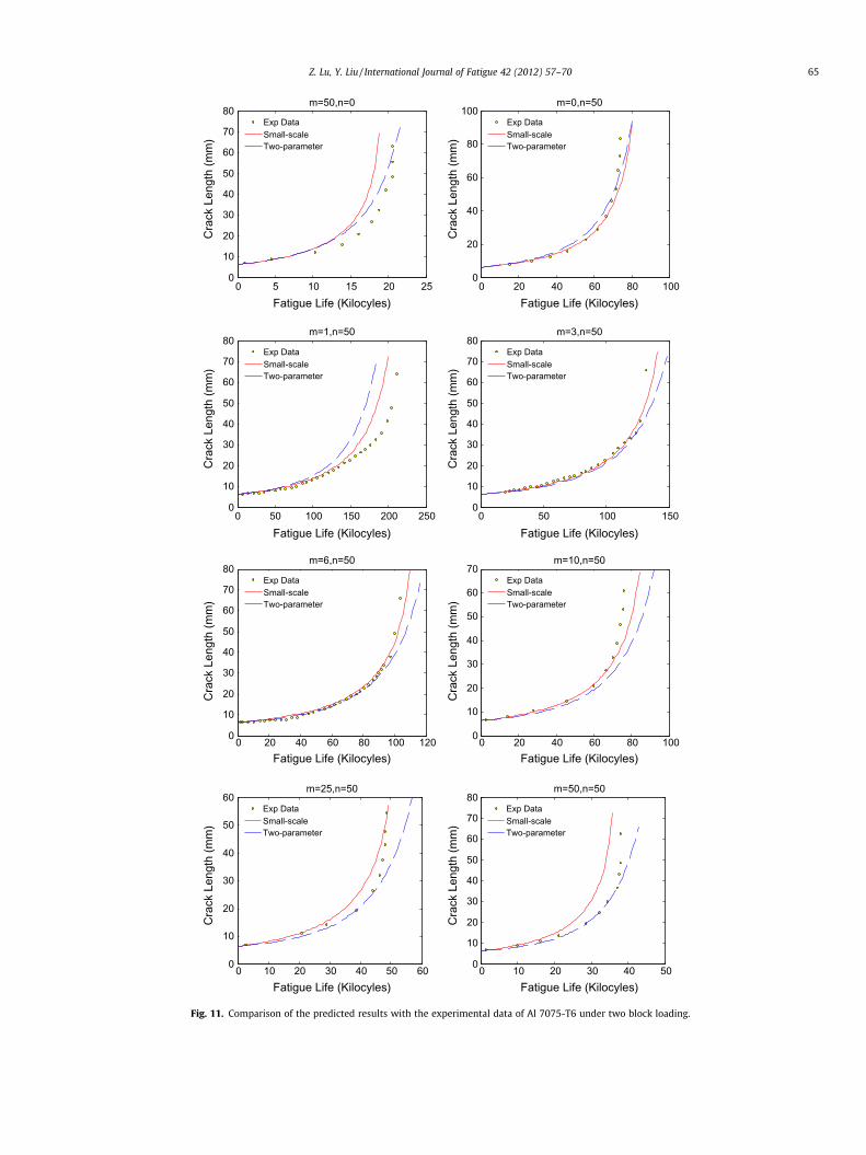
Fig. 10. Schematic illustration of the two block loading [17].


Figs. 4a–9a show the raw fatigue crack growth data as afunction of DK for Al 7075-T6 [13], Al 2024-T3 [13], Al 7050-T4571 [13], 300M steel [14], 4340 steel [15] and Ti–10V–2Fe–3Al [16], respectively. Using DKeq instead of DK, data under var-ious R-ratios can be consolidated into a single master curve. Figs.4b–9b show the fatigue crack growth data as a function of DKeq

using the two driving force approach and Figs. 4c–9c shows theplot for the small time scale model. It is seen that both ap-proaches yield a satisfactory results. For 4340 steel, the twodriving force model seems to catch crack growth curve better.The small time scale model overestimates the slope of the fati-gue crack growth rate curve. Detailed investigation for the smalltime scale formulation for high strength steel alloys needs fur-ther investigation.

0 5 10 15 20 250

10

20

30

40

50

60

70

80

Fatigue Life (Kilocyles)

Cra

ck L

engt

h (m

m)

m=50,n=0

Exp DataSmall-scaleTwo-parameter

0 20 40 60 80 1000

20

40

60

80

100


Cra

ck L

engt

h (m

m)

m=0,n=50


0 50 100 150 200 2500

10

20

30

40

50

60

70

80


Cra

ck L

engt

h (m

m)

m=1,n=50


0 50 100 1500

10

20

30

40

50

60

70

80


Cra

ck L

engt

h (m

m)

m=3,n=50


0 20 40 60 80 100 1200

10

20

30

40

50

60

70

80


Cra

ck L

engt

h (m

m)

m=6,n=50


0 20 40 60 80 1000

10

20

30

40

50

60

70


Cra

ck L

engt

h (m

m)

m=10,n=50


0 10 20 30 40 500

10

20

30

40

50

60

70

80


Cra

ck L

engt

h (m

m)

m=50,n=50


0 10 20 30 40 50 600

10

20

30

40

50

60


Cra

ck L

engt

h (m

m)

m=25,n=50


Fig. 11. Comparison of the predicted results with the experimental data of Al 7075-T6 under two block loading.


0

2

4

6

8

10

12

14

16

18

Block of loading

Stre

ss (

ksi)

σ1

σmin

σ2

n

Fig. 12. Block loading illustration.

0 20 40 60 800

10

20

30

40

50

60

70


Cra

ck L

engt

h (m

m)

Constant Amplitude Loading


MPa45.3

MPa95.68

min

1

==

σσ

0 50 100 150 2000

10

20

30

40

50

60

70


Cra

ck L

engt

h (m

m)

m=1,n=29


MPa43.103

MPa95.68

2

1

==

σσ

0 50 100 1500

10

20

30

40

50

60


Cra

ck L

engt

h (m

m)

m=1,n=29


MPa90.137

MPa95.68

2

1

==

σσ

Fig. 13. Comparison of the predicted results with the exp


4. Comparative study under variable amplitude loadings

4.1. Experimental data summary

In this part, experimental data on Al 7075-T6 and Al 2024-T3plate specimen with center through crack under different typesof variable amplitude loading are used to validate the proposedmodel. The experimental data are reported in [17] and [18].

A summary of the properties of the specimens used for the col-lected experimental data are listed in Table 4. For the two drivingforce model, the parameters C, a, and p in Eq. (2) are calibrated bycrack growth data under five different R-ratios in reference [13].The values are reported in Table 4.

0 20 40 60 80 100 1200

20

40

60

80

100


Cra

ck L

engt

h (m

m)

m=1,n=29


MPa54.76

MPa95.68

2

1

==

σσ

0 50 100 150 200 2500

10

20

30

40

50

60

70


Cra

ck L

engt

h (m

m)

m=1,n=29


MPa66.120

MPa95.68

2

1

==

σσ

0 100 200 300 4000

10

20

30

40

50

60

70

80


Cra

ck L

engt

h (m

m)

m=1,n=29


MPa43.103

MPa95.68

2

1

==

σσ

erimental data of Al 7075-T6 under overload loading.

Program P01

Program P04

0

2

4

6

8

10

12


Stre

ss (

ksi)

0 20 40 60 80 100 1200

20

40

60

80

100


Cra

ck L

engt

h (m

m)

P01


0

2

4

6

8

10

12

14


Stre

ss (

ksi)

0 20 40 60 80 1000

20

40

60

80

100


Cra

ck L

engt

h (m

m)

P04Exp DataSmall-scaleTwo-parameter

Program P09

Program P10

0

2

4

6

8

10

12

14

16


Stre

ss (k

si)

0 50 100 150 2000

20

40

60

80

100


Cra

ck L

engt

h (m

m)

P09


0

2

4

6

8

10

12

14


Stre

ss (

ksi)

0 50 100 1500

20

40

60

80

100


Cra

ck L

engt

h (m

m)

P10


Fig. 14. Model validation with spectrum data for Al 2024-T3 [17,18].


0 50 100 1500

10

20

30

40

50


Cra

ck L

engt

h (m

m)

m=1,n=50


MPa14.155

5.17MPa

2

1

==

σσ

0 20 400

10

20

30

40

50

60

70

Fatigue Life

Cra

ck L

engt

h (m

m)

m=1,n=


No OverloadOnly Underload

0 20 40 60 80 100 1200

10

20

30

40

50

60


Cra

ck L

engt

h (m

m)

m=1,n=50


MPa45.134

MPa31.03

2

1

==

σσ

Fig. 16. Model validation with overload–

0

4

8

12

16

20

24

0 5 10 15 20 25 30 35 40

Loading

Str

ess

(Ksi

)

1σ

2σ

Fig. 15. Loading illustration for overload–underload [17].


4.2. Comparison between model predictions and experimentalobservations

Extensive experimental data are collected from open literaturefor model validation. They are grouped into three categories: twoblock loading, spectrum loading and overload/underload loading.Details are shown below.

4.2.1. Al 7075-T6 under two block loadingExperimental data of Al 7075-T6 [17] under two block loading

and single overload spectrum are used for model validation. Aschematic illustration of the two block loading is shown in

0 50 100 150 2000

10

20

30

40

50

60

70


Cra

ck L

engt

h (m

m)

m=1,n=50


MPa14.155

MPa31.03

2

1

==

σσ

60 80 (Kilocyles)

50

MPa45.103

5.17MPa

2

1

==

σσ

0 20 40 60 805

10

15

20

25

30

35


Cra

ck L

engt

h (m

m)

m=1,n=50


MPa85.206

5.17MPa

2

1

==

σσ

underload data for Al 7075-T6 [17].


Fig. 10. m and n in Fig. 10 controls the number of cycles at the highamplitude and the low amplitude, respectively. Eight sets of exper-imental different block loadings are used for model validation andare plotted in Fig. 11. m and n values for each spectrum loading areshown in the legend. Predictions given by the two driving forcemodel and the small time scale model are plotted together.

To further investigate different model performance, a specialtwo block loading (i.e., single overload loading) is shown sepa-rately. The illustration of the single overload spectrum is shownin Fig. 12. The maximum stress values of the overload cycle andthe regular load cycle are shown as r1 and r2 in Fig. 12, respec-

0

4

8

12

16

20

24

0 5 10 15 20 25 30 35 40

Loading

Stre

ss (

Ksi

)

n

1σ

2σ

Fig. 17. Loading illustration for underload–overload [17].

0 20 40 60 80 100 1200

10

20

30

40

50


Cra

ck L

engt

h (m

m)

m=1,n=50


155.14MPa

5.17MPa

2

1

==

σσ

0 20 40 60 80 1005

10

15

20

25

30

35


Cra

ck L

engt

h (m

m)

m=1,n=50


206.85MPa

MPa5.17

2

1

==

σσ

Fig. 18. Model validation with underload

tively. Model predictions are compared with experimental datain Fig. 13 for six different overload ratios. r1 and r2 are listed inthe legend for different cases. According to the comparisons re-sults, it is seen that both the two driving force model and the smalltime scale model give satisfactory results, except for one loadingcase.

4.2.2. Al 2024-T3 under variable spectrum loadingDifferent variable spectrum loading of Al 2024-T3 is used to val-

idate the proposed model. Comparisons are shown in Fig. 14. Thefigure on the left side is the illustration of spectrum shape andthe figure on the right side is the model predictions with experi-mental data. A total of 13 spectrums are compared and only afew of them are shown here to save the space. For some cases,the proposed two driving force model gives a very good predictionand for some cases it seems to have a conservative prediction.

4.2.3. Al 7075-T6 specimen under underload/overload interactionsThis sub-task investigates the effect of underload/overload

interaction, which has been shown to be important for variableamplitude loading crack growth [19,20]. Two types of loading areused. The first the overload followed by an underload. A schematicplot of this type of loading is shown in Fig. 15. Model predictionsare compared with experimental data in Fig. 16. Another loadingtype is the underload followed by an overload. A schematic plotof this type of loading is shown in Fig. 17. Model predictions arecompared with experimental data for Al 7075-T6 in Fig. 18. Gener-ally, both models agree the experimental observation well.

0 50 100 1500

10

20

30

40

50

60

70


Cra

ck L

engt

h (m

m)

m=1,n=50


134.45MPa

31.03MPa

2

1

==

σσ

0 50 100 150 200 2500

10

20

30

40

50

60

70


Cra

ck L

engt

h (m

m)

m=1,n=50


155.14MPa

31.03MPa

2

1

==

σσ

–overload data for Al 7075-T6 [17].


5. Conclusions

This paper gives a comprehensive comparative study of the twodriving force approach and the previously developed small timescale fatigue model under constant amplitude loading. A modifiednew two driving force model is developed based on the concept ofinteraction of forward and reverse plastic zone under variableamplitude loading to include the overload/underload interactionssimilar to the small time scale model. Detailed comparison is per-formed to compare the applicability of the two driving force modeland the small time scale model for fatigue crack growth predictionunder constant amplitude loadings and variable amplitude load-ings. For both models, good agreements with experimental dataare observed for the loading history and materials collected inthe current investigation.

In future work, direct in situ testing is required to investigatecrack growth mechanism at the sub-cycle level in order to enhancethe physical significance of proposed small time scale model. Somepreliminary results have been shown under in situ SEM testing forthis purpose in [21]. Intrinsic threshold SIF value and the near-threshed crack growth need further investigation since theproposed methodology is mainly on the linear Paris regime. Inaddition, the current investigation is deterministic in nature anda probabilistic approach is more appropriate to handle theprediction errors/variability in the future study.

Acknowledgements

The research reported in this paper was supported by fundsfrom the NASA Ames Research Center (Contract No. NNX09AY54A,Project Manager: Dr. Kai Goebel) and by funds by funds from NAV-AIR under SBIR N68335-09-C-0265 (Project Manager: Dr. Rahman,Anisur). The support is gratefully acknowledged.

References

[1] Lu Zizi, Liu Yongming. Small time scale fatigue crack growth analysis. Int JFatigue 2010;32(8):1306–21.

[2] Sadananda K, Vasudevan AK. Multiple mechanisms controlling fatigue crackgrowth. Fatigue Fract Eng Mater Struct 2003;26(9):835–45.

[3] Vasudevan AK, Sadananda K. Application of unified fatigue damage approachto compression–tension region. Int J Fatigue 1999;21:S263–73.

[4] Kujawski Daniel. A new (DK + Kmax)0.5 driving force parameter for crackgrowth in aluminum alloys. Int J Fatigue 2001;23(8):733–40.

[5] Kujawski Daniel. A fatigue crack driving force parameter with load ratioeffects. Int J Fatigue 2001;23(Suppl. 1):239–46.

[6] Noroozi AH, Glinka G, Lambert S. A two parameter driving force for fatiguecrack growth analysis. Int J Fatigue 2005;27(10–12):1277–96.

[7] Newman JC, James MA, Zerbst U. A review of the CTOA/CTOD fracture criterion.Eng Fract Mech 2003;70:371–85.

[8] Srinivansan K, Kolednik O, Siegmund T. A study on crack propagation inheterogeneous elastic–plastic solids. In: Nielson F, editor. The 15th Europeanconference on fracture, Stockholm; 2004.

[9] McClung RC. Crack closure and plastic zone sizes in fatigue. Fatigue Fract EngMater Struct 1990;14(4):455–68.

[10] Dinda Sudip, Kujawski Daniel. Correlation and prediction of fatigue crackgrowth for different R-ratios using Kmax and DK+ parameters. Eng Fract Mech2004;71(12):1779–90.

[11] Stoychev Stoyan, Kujawski Daniel. Analysis of crack propagation using[Delta]K and Kmax. Int J Fatigue 2005;27(10–12):1425–31.

[12] Maymon G. A ‘unified’ and a (DK � Kmax)1/2 crack growth models for aluminum2024-T351. Int J Fatigue 2005;27(6):629–38.

[13] Forman FG, Shivakumar V, Cardinal JW, Williams LC, McKeighan PC. Fatiguecrack growth database for damage tolerance analysis. US Department ofTransportation, Federal Aviation Administration; 2005. p. 126.

[14] Chang T, Guo W. Effects of strain hardening and stress state on fatigue crackclosure. Int J Fatigue 1999;21(9):881–8.

[15] Noroozi AH, Glinka G, Lambert S. A study of the stress ratio effects on fatiguecrack growth using the unified two-parameter fatigue crack growth drivingforce. Int J Fatigue 2007;29(9-11):1616–33.

[16] Jha SK, Ravichandran KS. Effect of mean stress (stress ratio) and aging onfatigue-crack growth in a metastable beta titanium alloy, Ti–10V-2Fe–3Al.Metall Mater Trans 2000;31A:703–14.

[17] Porter TR. Method of analysis and prediction for variable amplitude fatiguecrack growth. Eng Fract Mech 1972;4:717–36.

[18] Patankar R. Modeling fatigue crack growth for life extending control. In:Mechanical engineering, vol. Doctor: Pennsylvania State University; 1999.

[19] Mikheevskiy S, Glinka G. Elastic–plastic fatigue crack growth analysis undervariable amplitude loading spectra. Int J Fatigue 2009;31(11–12):1828–36.

[20] Skorupa M. Load interaction effects during fatigue crack growth under variableamplitude loading – a literature review. Part II: Qualitative interpretation.Fatigue Fract Eng Mater Struct 1998;22:905–26.

[21] Zhang W, Liu Y. In-situ optical microscopy/SEM fatigue crack growth testing ofAl7075-T6. In: Aircraft airworthiness & sustainment, Austin, TX 2010.

a comparative study between a small time scale model and the two driving force model for fatigue...

Documents