A CAPITAL MARKETSVIEW OF MORTGAGESERVICING RIGHTS

SIMON P. B. ALDRICHD I R E C T O R

C D C M O R T G A G E C A P I T A L9 W. 5 7 T H S T . N Y, N Y 1 0 0 1 9

S I M O N @ C D C N A . C O M( 2 1 2 ) 8 9 1 - 6 1 6 3

WILLIAM R. GREENBERGD I R E C T O R

C D C M O R T G A G E C A P I T A L9 W. 5 7 T H S T . N Y, N Y 1 0 0 1 9

G R E E N B E R @ C D C N A . C O M( 2 1 2 ) 8 9 1 - 6 2 2 0

BROOK S. PAYNERM A N A G I N G D I R E C T O R

C D C M O R T G A G E C A P I T A L9 W. 5 7 T H S T . N Y, N Y 1 0 0 1 9

PAY N E R @ C D C N A . C O M( 2 1 2 ) 8 9 1 - 6 2 8 1

ABSTRACT

A consistent framework for the valuation and hedging of mortgage servicing rights (MSR) using theIO securities markets is described. The similarities and differences between the mortgage servicingand IO securities markets are explored. After a discussion of some of the characteristics and risksinherent in an investment in mortgage servicing rights, we use option pricing techniques to look atmortgage servicing valuation in the context of IO market valuations. Results showing therelationships between these two markets are displayed. Issues regarding the hedging of mortgageservicing, again relative to the IO market, are also discussed.

S U B M I T T E D T O “ T H E J O U R N A L O F F I X E D I N C O M E ” O C T O B E R 2 0 0 0V e r s i o n 7 ; 1 0 / 2 0 / 0 0

2

I . INTRODUCTION

After opening its New York office in 1990, Caisse Des Depots et Consignations, “CDC,” quicklybecame recognized as one of the leading investors in the mortgage-backed securites markets.Developing its own interest-rate and prepayment models, CDC employed OAS and other option-pricing techniques from the earliest days. In 1994, CDC leveraged its expertise in the MBS marketsand became an investor in the market for mortgage servicing rights (MSR’s). Through the years, aswe have traded and monitored both the MBS market, specifically mortgage derivatives, and themortgage servicing market, we have had the opportunity to think very hard about the difficult issuesinvolved in hedging and pricing mortgage servicing compared to the hedging and pricing of MBS.This paper is the result of those experiences. We hope that mortgage-backed securities traders andinvestors, particularly participants in the IO/PO market, will read this paper and learn somethingabout mortgage servicing rights and the issues surrounding that peculiar asset. Additionally, we hopethat mortgage servicers will read this paper and learn about the way that IO/PO traders andinvestors look at the world and the consequences of that view for the mortgage servicing market.

Over the last several years, the market for mortgage servicing rights has undergone a significanttransformation as the trend towards consolidation in the industry continues. There are now nineservicers with over $100 billion in servicing while the top ten servicers combined together represent41.6% of the market1. The objective of consolidation among these mega-servicers is to benefit fromeconomies of scale. Profitability should increase because marginal cost is much less than averagecost and marginal revenue should increase from greater cross-selling opportunities. The concept ofthe “customer for life” and the profits to be garnered from him have driven the competition betweenthe mega-servicers to new levels as market prices for MSR’s are at multiples that have not been seenin many years, if ever.2 As a consequence, smaller servicers have largely chosen to sell to the mega-servicers and recognize any gains in current earnings thereby satisfying management and shareholderswhile eliminating the interest rate risk associated with holding the asset. This has been particularlytrue of so-called pre-FAS122 servicing, which was booked at zero value and therefore was effectivelynot on the balance sheet.3 Even as smaller originators have sold most of their servicing, more recentoriginations of on-balance-sheet servicing have been brought to market as well. Anotherconsequence of the consolidation trend is that smaller servicers are becoming more broker-like,originating loans and selling their servicing on a flow basis to the very largest servicers.

Another development in the mortgage servicing market in recent years is the recognition of thesubstantial market risks inherent in owning MSR’s. Many market participants still employ a staticanalysis of risk, which significantly understates the true exposure. The use of dynamic interest rateand prepayment models gives a more realistic picture of the risks involved in owning MSR’s,although these models are still deficient in practice as significant differences between theoretical andmarket valuations can persist over long periods of time. 1 Mortgage Servicing News, Volume 4, No. 6, June 2000

2 The price of servicing is often expressed as a multiple of the servicing strip. For example, a 25 basis point strip of MSR’spriced at 200 basis points (up front) has a multiple of 8.0.

3 Pre-FAS 122 servicing is servicing which was originated prior to the adoption of FAS 122.

3

Furthermore, the imminent adoption of FAS133 has focused much attention on the issues of valuingand hedging MSR’s. The details of the requirements of FAS133 are too complex to describesuccinctly here. The implications of the new guideline, however, are easy to understand. Prior to theadoption of FAS 133, the accounting rules for MSR’s are that they are marked at Lower Of Cost OrMarket (LOCOM) and associated hedges are marked to market. To the extent that rates rise, it isonly possible to mark the MSR’s up to the cost paid for those rights and no higher. Thus, there is anaccounting distortion relative to the economics. The amount by which the market value of theservicing exceeds the cost is sometimes called “cushion”. If certain requirements are satisfied,“hedge accounting” can be used. Under hedge accounting rules, the value of the servicing can bemarked up above its cost to the extent, and only to the extent, that it offsets losses on derivativehedge instruments which are marked to market. Thus, in a rising rate environment, MSR’s can bewritten up to offset the losses on the hedges, resulting in very little p&l volatility. Under FAS 133,hedge accounting is still attainable but under different and more stringent requirements. Evenassuming that these requirements can be met, the new rule states that MSR’s are essentially marked tomarket, as are the derivative hedges. The result is that any p&l volatility between the market value ofthe hedges and the market value of the servicing flows through to current earnings4. For the mega-servicers who own hundreds of billions of dollars in servicing, this volatility could potentially be inthe neighborhood of $100-$150 million per quarter5. For publicly traded companies whose earningsare in the $500 million-$1 billion per quarter range, the earnings volatility due to mortgage servicingis very significant. Thus, the question of how to very precisely hedge MSR’s has become cruciallyimportant.

The risks associated with mortgage servicing rights are similar in many respects to those associatedwith Interest-Only (IO) securities in the mortgage-backed securities markets. The biggest risk isprepayment risk. When mortgage rates decline, prepayments increase, and the value of IO’s andmortgage servicing alike decline. IO’s, however, are securities which are actively traded in a relativelyliquid market. The prices of most Trust IO’s are easy to obtain. Not so with MSR’s since the marketis nowhere near as liquid. MSR’s are not securities and do not have uniform characteristics like IOstrips. Furthermore, the characteristics of the investors in IO securities are very different from theinvestors in mortgage servicing. As described above, mortgage servicing investors are primarilyinterested in earning fees from servicing the customer, collecting loan payments, and processing theclerical aspects of the business. IO investors have no direct interest in the customer, but insteadhope to extract a spread between the income generated from the security and the cost of funding.They do not care about the underlying customer, can never sell him anything (nor do they want to),

4 Another accounting possibility exists whereby hedge accounting treatment is not sought and earnings volatility insteadflows through equity. In this case, the servicing is accounted for on a LOCOM basis and the hedge instruments, whichmight include cash instruments, are held in an “available for sale” account. In a falling rate environment, the servicingdeclines in value, which flows through to income, and the hedges increase in price, which flows through to equity. In orderto flatten out the changes in value in the equity, the hedge instruments must be sold and new hedge instruments will needto be purchased. This results in no net change to equity and no net change to income. In a rising rate environment,servicing prices are capped, so nothing flows through to income, while hedge values decline in value. In this case, the p&lvolatility due to LOCOM hedging flows through to equity.

5 Even if the interest rate risk of servicing is hedged perfectly, spread movements between the servicing and its hedge stillare significant. If the spread moves 100 basis points, the spread duration is 3.5 years, the market value of servicing is $3 to$4 billion, then the volatility is conservatively estimated to be $100-$140 million. As shown below, 100 basis points hasbeen a relatively small spread movement on an historical basis.

4

and since the IO is a security, they do not have any of the accounting difficulties that servicerswrestle with every day. Another salient difference is that mortgage servicers can sometimes recapturea loan that prepays, thereby reducing the loss realized from prepayment.6 In contrast, once a loanpays off, the IO investor realizes his loss immediately.

Nevertheless, since the financial risks are so similar – indeed, a subset of the mortgage servicingcashflows is economically identical to Trust IO’s – it makes sense to try to extract information aboutMSR’s from the IO market. This has been the philosophy underlying CDC’s valuation and hedgingof mortgage servicing over the years. It is our view that through the application of some of the mostcommonly used methods in the IO market to determine relative value, information regarding thevaluation and hedging of mortgage servicing can be extracted. The purpose of this paper is todescribe a consistent method of looking at the valuation of MSR’s in the context of the IO market(using option pricing techniques) and to share some of the more interesting results which we haveobserved regarding the relationship between these two markets. In this paper, we refer to thisapproach as the Capital Markets approach to valuing and hedging MSR’s.

The remainder of this paper is organized as follows. In Section II, the characteristics of mortgageservicing rights are more fully described. In Section III, the risks associated with mortgage servicingare outlined, and the differences and similarities to the IO market are also described. In Section IV,the way that CDC has used the IO market to extract information regarding servicing is described.Sections V, VI, and VII contain the results of the “OAS” analysis and will hopefully provide newinsights to the reader regarding the current state of the mortgage servicing market as well as thevaluation and hedging of mortgage servicing rights. Finally, in Section VII, a summary of the paperis provided and conclusions are drawn.

II . CHARACT ERISTICS OF MORTGAGE SERVICING

Mortgage servicing rights, although they are not securities, grant the owner the right to receivecertain cashflows and encumber the owner with the responsibility to pay certain other cashflows. Avery simple model divides the servicing cashflows into six separate components: the servicing fee, thenet cost to service, the float on taxes and insurance, the float on principal and interest, the gain fromprepayments, and the loss due to compensating interest. Each of these is taken up in turn below.

The mortgage servicer actually receives the gross servicing fee but only gets to retain the net servicingfee. The gross servicing fee is the difference between the coupon on the underlying mortgage andthe coupon on the loan which has been purchased by an investor such as a Government SponsoredEnterprise (“GSE”) or by a private investor. The net servicing fee is that amount of the grossservicing fee that is left after paying the GSE’s guaranty fees and other fees. Typically, forconventional servicing, the net servicing fee is about 25 bps (0.25%) of the balance of the underlyingloan; for GNMA servicing, the net servicing fee is typically 44 bps.

6 The ability to recapture a prepaying loan implies that servicing values should account this feature which is missing fromIO valuations. The fact that origination volumes typically increase during periods of high prepayments leads to the notionof a “natural hedge” for servicers who also have an origination business. We discuss the implications of recapturingprepaying loans below.

5

It is important to note that the servicing fee retained by the servicer is not necessarily the same forevery loan. If the servicing fees on the loans comprising a pool are different, then at the pool level,the net servicing fee realized by the servicer can increase if the lower service fee loans pay off early,or it can decrease if the higher service fee loans pay off sooner. Typically, the higher service feeloans correspond to higher mortgage rates and so it is more common for these loans to pay offsooner and the servicing fee typically declines over time. In the securities market, this is similar to aso-called weighted average coupon IO (“WAC IO”).

The second component is the net cost to service. That is, unlike the IO investor, the servicer isactually required to spend money to go out and collect the service fee. Systems and people arerequired to do the billing, collection, processing, and customer service associated with mortgagepayments. This is another big difference between the IO buyer and the servicing buyer. Getting ahandle on the actual costs a company faces in servicing its loans is one of the biggest challenges itfaces. The prices at which portfolios of servicing rights are exchanged imply a certain cost to service– this subject will be returned to later. It is also interesting to question whether it is the average costto service the loans or the marginal cost which is relevant and for which purposes. In evaluating thetotal economics of a servicing business, it makes sense to use the average cost per loan in calculatingprofitability. For pricing portfolios of servicing, however, it makes sense to use the marginal cost,since that most accurately reflects the cost of adding more loans to an existing platform.

Every portfolio has at least some delinquent loans. When a loan becomes delinquent, late chargesaccrue. To the extent that the servicer can collect these late fees, they are another source of income.Typically, a servicer might expect to collect 80% or so of the late charges owed. Additionally,however, as more loans become delinquent, more time and effort has to be spent on that loan tocollect the late fee and to make the loan current again. While there is some extra income associatedwith loans becoming delinquent, it is never a good thing for too many loans to become delinquent asthe cost to service rises and principal losses may accumulate. Servicing advances of late paymentsalso increase costs, although for GSE guaranteed loans, these costs will generally be reimbursed at alater date by the agencies, assuming that there was no fraud in the origination of the loan. There issometimes an assortment of other fees which are assessed sporadically and which accrue to thebenefit of the servicer.

Our approach has been to combine these components of the cost to service together with the benefitof late charges and other ancillary income. For example, it might cost $40 per loan per year toservice a loan and the servicer might realize $30 per loan per year in late charges and ancillaryincome, for a net $10 cost. Alternatively, the servicer might realize $60 per loan per year in ancillaryincome and it might only cost $25 to service for a net gain of $35 per loan per year. Most servicersagree that, after taking all of these factors into account, the industry marginal cost to service, net ofancillary and late charges, is probably somewhere in the $0-$20 net cost range. As we review later,this marginal cost is embedded in our analysis of the pricing of servicing portfolios that areexchanged in the market.

Another source of information on the net servicing cost is the sub-servicing market. Sub-servicerswill perform the servicing function in return for a fee, usually on a per loan basis. It is interesting tonote, however, that at the time of this writing, the market for sub-servicing requires that the sub-servicer get paid a fee closer to $70 than to $20 per loan per year net of ancillary income and latecharges. This may imply a difference between sub-servicers’ and primary servicers’ cost to serviceand may help explain why the sub-servicing market has been slow to become substantial. The largest

6

subservicers have substantially smaller servicing portfolios than the largest primary servicers so thattheir average cost is probably much larger than that of the typical primary servicer. If a primaryservicer’s own cost is substantially below what he can get in the sub-servicing market then hisincentive to use a sub-servicer will be low.

In addition to discussing cost assumptions with other servicers, we have asked brokers about theirviews of costs and also observed the costs implied in market prices of servicing portfolios.Although, in this paper, we argue that option pricing techniques are the most reliable for pricing andhedging portfolios of mortgage servicing, many servicing market participants use a static pricingmethodology – with Bloomberg median prepayment speeds and a single static discount rate andcrediting rate. Indeed, every quarter CDC asks two servicing brokers to estimate market prices forCDC’s portfolios of servicing rights, the brokers provide, in addition to price estimates, theirassumptions regarding the cost to service and ancillary income and late charges. One broker hasindicated that the cost to service net of ancillary income is $15 per loan per year, but not includinglate charges. If late charges are included this number should be in the $10-$5 per loan per year in netcosts. A second broker indicates that the total cost to service, net of late charges and ancillaryincome is $10 per loan per year. As further support, CDC’s own experience in trying to predict tradeprices on portfolios of servicing using the static method of pricing servicing portfoilios– usingBloomberg median prepayment rates and some static discount rate – actually works quite well whenthe net cost to service is in the $5-$15 per loan per year range. Throughout this paper, we use $10per loan per year cost to service, net of ancillary income and late fees.

The third component is the income generated from the float on taxes and insurance. A portion ofthe mortgage payment made by a homeowner typically includes an amount to pay taxes on theproperty and to pay for insurance. The servicer collects these monies from the homeowners andpays them to the appropriate entities. However, the collecting entities do not all expect the money atthe same time; the servicer holds these funds and invests them for some period of time. Differentstates have different requirements as to when and how often the taxes must be remitted. Servicingfrom a state that only requires the taxes to be remitted once per year is more valuable than servicingfrom a state that requires remittances more than once per year, everything else being equal.Additionally, some states require that the servicer credit the mortgagor with a certain rate of intereston these balances. Typically, we use LIBOR as the crediting rate for the float income on T&I. Oneimportant feature of T&I float is that it grows over time as a percent of the remaining loan balance.That is, as long as a homeowner owns his home, he has to pay taxes and insurance based on thevalue of the house, regardless of the principal balance outstanding on the loan.

Similarly, the servicer is able to invest the principal and interest payments which the homeownermakes before remitting to the agencies. The exact number of days that the servicer can invest thismoney depends on the remittance program of the GSE. The number of days of possible investmentrange from 0 in “Actual/Actual” programs to as much as 45 days depending on when thehomeowner makes his monthly payment. 7

7 For a description of various remittance programs and the valuation of the float components, see “Mortgage PrepaymentFloat”, The Journal of Fixed Income, Vol.7 No. 4, March 1998.

7

There is also the possibility of a further gain on the float components due to prepayments. When aloan prepays, the servicer invests the loan balance until the remittance date and earns interest on thebalance. However, there is also the possibility that the servicer loses money on prepayments, whichis the last of the 6 servicing components. Depending on the servicing remittance type, the servicermay be required to remit to the agencies a full month of interest on each underlying loan, regardlessof when that loan has paid off during that month. If a loan pays off in the middle of a month, thehomeowner only pays the pro-rata share of the interest; the servicer must make up the rest. This isknown in the securities markets as compensating interest.

We have built a simple model of mortgage servicing cashflows which incorporates all of thecomponents described above. Other models can be used which have more inputs, but we believethat most of those additional components for which we do not have explicit inputs can be includedin the net cost to service or in one of the other components. The explicit model is described below.

At time t the cashflow from a mortgage servicing portfolio can be written as

)()()()()()()( tLtGtTItPItCtStCF +++++= , (1)

where, )(tS is the contribution due to the IO Strip, )(tC is the contribution due to the Net MarginalCost, )(tPI is the contribution due to the Scheduled P&I Float, )(tTI is the contribution due to theT&I Float, )(tG is the contribution due to the Prepay Gain component, and )(tL is thecontribution due to the Prepay Loss component. Explicitly, these components are given by thefollowing expressions:

,)()()(

,360

))(()(

,360

)()(

,)0()0(

121)()(

,360

)()(

),()(

),(12

)(

00 tB

tBNtN

dwstPItL

dtPIrtG

NTIitNrtTI

dtPIrtPI

tcNtC

tBstS

lossunsched

unschedunschedpi

t

ti

schedschedpi

=

−=

=

���

� +=

=

=

=

(2)

and where s is the annualized net servicing fee (e.g. 25 bps), B(t) is the balance of the pool at time t, cis the cost to service per loan net of ancillary income and late charges, per month (e.g. $10 net costwould be –0.8333 dollars per loan). dsched, dunsched, dloss, represent the number of days the servicer isentitled to hold the scheduled principal and interest payments, the number of days the servicer is

8

entitled to hold the unscheduled principal payments, and the number of days of compensatinginterest necessary to make up one entire month of interest which must be remitted to the agency,depending on the remittance type and the day of the month the mortgagor pays off his loan. Therates rpi, rti, represent the crediting rate for principal and interest and for taxes and insurance for thefloating rate components. These numbers are typically 1-month LIBOR based and may or may notinclude a spread. PIsched and PIunschedi represent the scheduled and unscheduled principal and interestpayments, which are projected from CDC’s interest rate and prepayment models, given theunderlying mortgage characteristics. N(t) is the number of loans outstanding at time t; N(0) is thenumber of loans at t=0, or the original number of loans. The inflation rate, i, represents the rate atwhich T&I payments grow. The quantity TI(0) is equal to the T&I constant multiplied by the stateT&I factor. The gross wac of the underlying mortgage is denoted by w. Finally, B0(t) is the projectedbalance of the mortgage pool, using the interest rate and prepayment models, assuming 0 CPR. Thisquantity is used in our model to project the number of loans remaining in the pool.

III . RISKS ASSOCIAT ED WIT H MORTGAGE SERVICING

There are basically three main risks associated with owning mortgage servicing rights: operationalrisk, interest rate risk, and prepayment risk. Each of these is taken up in turn below.

Mortgage servicing, as distinct from an investment in a security, requires the owner to deploysubstantial resources in order to collect and process the promised cashflows. The risks due to theoperational side of the servicing business are of an entirely different nature than the financial marketrisks associated with interest rates and prepayment rates. For instance, in making loans and retainingthe servicing, there is the possibility that the initial mortgage was made based on fraudulentinformation. In the case of GSE guaranteed loans, if the mortgagor defaults on the property, theagency will not reimburse the servicer for advances made to the security holders. Even if themortgage was made properly, if certain files relating to the loan origination become lost or misplaced,then the servicer might not be reimbursed for any losses relating to that particular loan.Furthermore, if a mortgagor defaults on a properly made loan, then the servicer will typically have toadvance the funds to the agencies. Even though this money is eventually repaid to the servicer whenthe property is sold, the servicer must bear the cost of financing the advance. The number ofdelinquent loans could increase which, even if the servicer is able to collect a late fee and the loancures itself, requires more time and effort on the part of the company to make sure the monies arecollected. These sorts of risks are difficult to quantify in the model presented above and to theextent they are uncorrelated with interest rates will have little or no impact on hedge ratios.

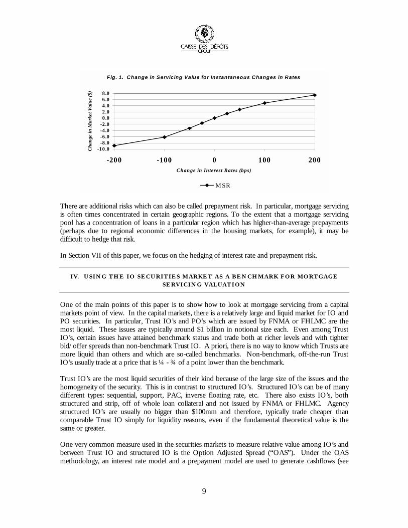
Other risks associated with owning mortgage servicing rights are prepayment risk and interest raterisk. It is sometimes difficult to separate the two since prepayments and interest rates are correlated.As interest rates (mortgage rates) fall, prepayments rise, and the value of the servicing fee declines.Furthermore, since mortgage servicing contains the P&I and T&I float components, thesecomponents are more valuable when rates are high and less when rates are low. The change in valueof a sample mortgage servicing portfolio for instantaneous changes in interest rates is shown inFigure 1, based on the model described in Section II and CDC’s prepayment and interest ratemodels. The profile shown in Figure 1 is a clearly IO-like profile, where the value of the assetincreases when interest rates increase and decreases as rates decrease. In the Figure, the yield curve isassumed to make parallel shifts.

9

Fig. 1. Change in Servicing Value for Instantaneous Changes in Rates

-10.0-8.0-6.0-4.0-2.00.02.04.06.08.0

-200 -100 0 100 200Change in Interest Rates (bps)

Chan

ge in

Mar

ket V

alue

($)

MSR

There are additional risks which can also be called prepayment risk. In particular, mortgage servicingis often times concentrated in certain geographic regions. To the extent that a mortgage servicingpool has a concentration of loans in a particular region which has higher-than-average prepayments(perhaps due to regional economic differences in the housing markets, for example), it may bedifficult to hedge that risk.

In Section VII of this paper, we focus on the hedging of interest rate and prepayment risk.

IV. USING THE IO SECURITIES MARKET AS A BENCHMARK FOR MORTGAGESERVICING VALUATION

One of the main points of this paper is to show how to look at mortgage servicing from a capitalmarkets point of view. In the capital markets, there is a relatively large and liquid market for IO andPO securities. In particular, Trust IO’s and PO’s which are issued by FNMA or FHLMC are themost liquid. These issues are typically around $1 billion in notional size each. Even among TrustIO’s, certain issues have attained benchmark status and trade both at richer levels and with tighterbid/offer spreads than non-benchmark Trust IO. A priori, there is no way to know which Trusts aremore liquid than others and which are so-called benchmarks. Non-benchmark, off-the-run TrustIO’s usually trade at a price that is ¼ - ¾ of a point lower than the benchmark.

Trust IO’s are the most liquid securities of their kind because of the large size of the issues and thehomogeneity of the security. This is in contrast to structured IO’s. Structured IO’s can be of manydifferent types: sequential, support, PAC, inverse floating rate, etc. There also exists IO’s, bothstructured and strip, off of whole loan collateral and not issued by FNMA or FHLMC. Agencystructured IO’s are usually no bigger than $100mm and therefore, typically trade cheaper thancomparable Trust IO simply for liquidity reasons, even if the fundamental theoretical value is thesame or greater.

One very common measure used in the securities markets to measure relative value among IO’s andbetween Trust IO and structured IO is the Option Adjusted Spread (“OAS”). Under the OASmethodology, an interest rate model and a prepayment model are used to generate cashflows (see

10

Section II). These cashflows are discounted to their present value again using the interest rate model.The option-adjusted spread, OAS, is that spread which must be added to every discount rate suchthat the sum of the discounted cashflows equals the market price. As such, the OAS is a measure ofhow much extra yield over the reference discount factors an investor earns by holding the security.8 9

IO market participants often talk about relative value between structured IO and Trust IO in termsof OAS. That is, off-the-run Trust IO will trade approximately 50 basis points of OAS cheap to thebenchmark of that issue. Other kinds of sequential or support IO might trade 100 to 200 basispoints of OAS cheap to the benchmark. Inverse floating rate IO’s might trade 300-1000 bps cheapto the benchmark.

It has been our approach to treat mortgage servicing as just another structured IO which should bevalued at some spread to the benchmark Trust IO. Furthermore, it is our view that by consideringonly the difference in OAS between servicing and Trust IO’s, the model dependence introducedthrough using particular interest rate and prepayment models (e.g. CDC’s) is greatly reduced. That is,while the details of the results presented here might change slightly based on a different prepaymentor interest rate model, the general trends and conclusions would still hold true.

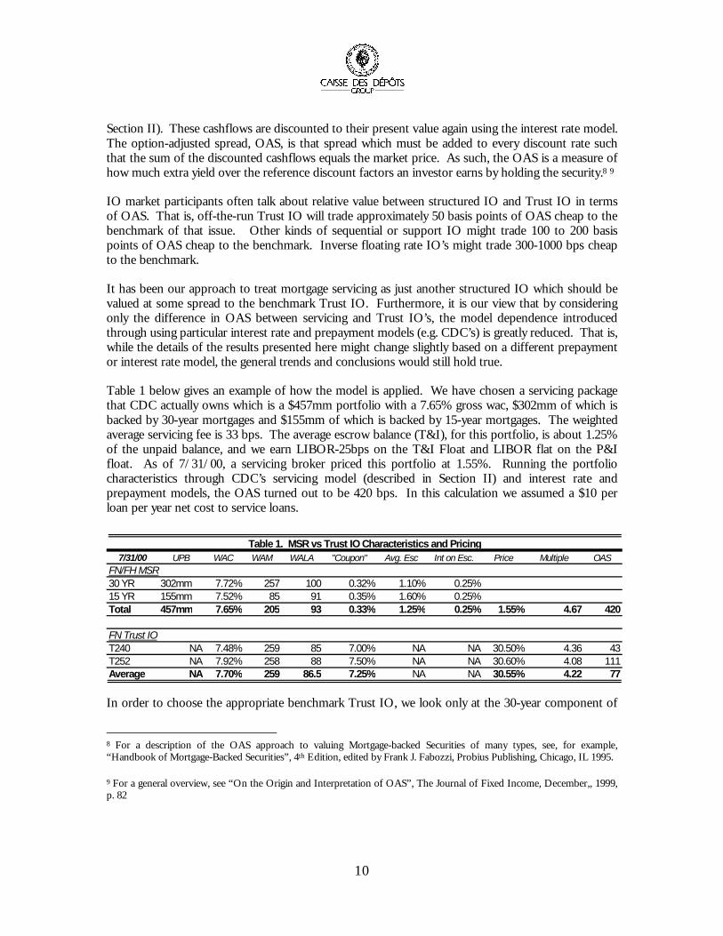
Table 1 below gives an example of how the model is applied. We have chosen a servicing packagethat CDC actually owns which is a $457mm portfolio with a 7.65% gross wac, $302mm of which isbacked by 30-year mortgages and $155mm of which is backed by 15-year mortgages. The weightedaverage servicing fee is 33 bps. The average escrow balance (T&I), for this portfolio, is about 1.25%of the unpaid balance, and we earn LIBOR-25bps on the T&I Float and LIBOR flat on the P&Ifloat. As of 7/31/00, a servicing broker priced this portfolio at 1.55%. Running the portfoliocharacteristics through CDC’s servicing model (described in Section II) and interest rate andprepayment models, the OAS turned out to be 420 bps. In this calculation we assumed a $10 perloan per year net cost to service loans.

7/31/00 UPB WAC WAM WALA "Coupon" Avg. Esc Int on Esc. Price Multiple OASFN/FH MSR30 YR 302mm 7.72% 257 100 0.32% 1.10% 0.25%15 YR 155mm 7.52% 85 91 0.35% 1.60% 0.25%Total 457mm 7.65% 205 93 0.33% 1.25% 0.25% 1.55% 4.67 420

FN Trust IOT240 NA 7.48% 259 85 7.00% NA NA 30.50% 4.36 43T252 NA 7.92% 258 88 7.50% NA NA 30.60% 4.08 111Average NA 7.70% 259 86.5 7.25% NA NA 30.55% 4.22 77

Table 1. MSR vs Trust IO Characteristics and Pricing

In order to choose the appropriate benchmark Trust IO, we look only at the 30-year component of

8 For a description of the OAS approach to valuing Mortgage-backed Securities of many types, see, for example,“Handbook of Mortgage-Backed Securities”, 4th Edition, edited by Frank J. Fabozzi, Probius Publishing, Chicago, IL 1995.

9 For a general overview, see “On the Origin and Interpretation of OAS”, The Journal of Fixed Income, December,, 1999,p. 82

11

the servicing. In this example, the 30-year wac and wam are 7.72% and 257 months, respectively.These parameters are about halfway between FNMA Trust 240 and FNMA Trust 252. Thecharacteristics for those two trusts are also shown in Table 1; the average wac is 7.70% and theaverage wam is 258.5 months, which is pretty close to the 30-year servicing. Each of the Trust IO’swas run through CDC’s models, using market prices, to obtain OAS’s of 43 bps and 111 bps,respectively. The average OAS of the two Trusts is 77 bps. Thus, as of the end of July 2000, thisservicing package was valued at 343 bps cheap relative to Trust IO.10

It is interesting in this analysis to also look at a comparison of the pricing “multiples”. The multipleis simply the price of the asset divided by the coupon. As seen in Table 1, the servicing multiple isgreater, by about 0.45, than the Trust IO multiple. One might claim that servicing is rich relative toTrust IO just because the multiple is larger. This is not true. Because the floating rate components,T&I and P&I float, contribute about 30% to the value of a servicing package but do not increase thecoupon, the multiple on the overall servicing package is naturally higher than that on just the stripportion. Indeed, the servicing is 343 bps cheap on an OAS basis.

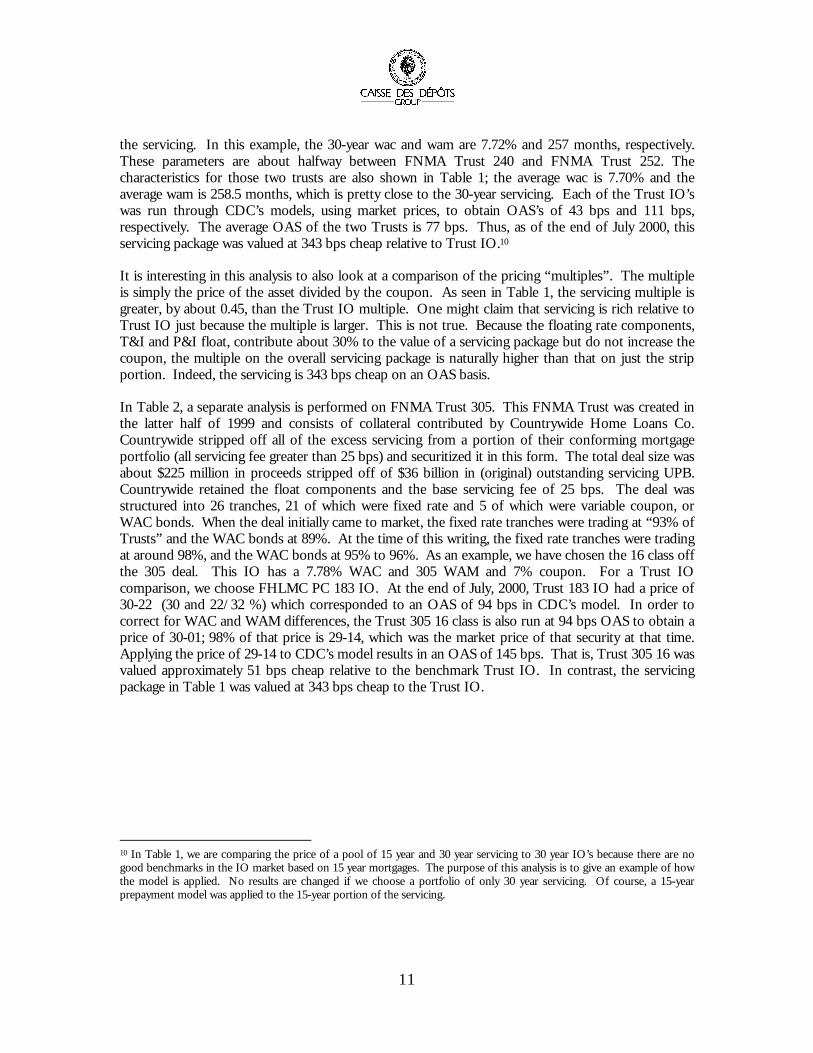
In Table 2, a separate analysis is performed on FNMA Trust 305. This FNMA Trust was created inthe latter half of 1999 and consists of collateral contributed by Countrywide Home Loans Co.Countrywide stripped off all of the excess servicing from a portion of their conforming mortgageportfolio (all servicing fee greater than 25 bps) and securitized it in this form. The total deal size wasabout $225 million in proceeds stripped off of $36 billion in (original) outstanding servicing UPB.Countrywide retained the float components and the base servicing fee of 25 bps. The deal wasstructured into 26 tranches, 21 of which were fixed rate and 5 of which were variable coupon, orWAC bonds. When the deal initially came to market, the fixed rate tranches were trading at “93% ofTrusts” and the WAC bonds at 89%. At the time of this writing, the fixed rate tranches were tradingat around 98%, and the WAC bonds at 95% to 96%. As an example, we have chosen the 16 class offthe 305 deal. This IO has a 7.78% WAC and 305 WAM and 7% coupon. For a Trust IOcomparison, we choose FHLMC PC 183 IO. At the end of July, 2000, Trust 183 IO had a price of30-22 (30 and 22/32 %) which corresponded to an OAS of 94 bps in CDC’s model. In order tocorrect for WAC and WAM differences, the Trust 305 16 class is also run at 94 bps OAS to obtain aprice of 30-01; 98% of that price is 29-14, which was the market price of that security at that time.Applying the price of 29-14 to CDC’s model results in an OAS of 145 bps. That is, Trust 305 16 wasvalued approximately 51 bps cheap relative to the benchmark Trust IO. In contrast, the servicingpackage in Table 1 was valued at 343 bps cheap to the Trust IO.

10 In Table 1, we are comparing the price of a pool of 15 year and 30 year servicing to 30 year IO’s because there are nogood benchmarks in the IO market based on 15 year mortgages. The purpose of this analysis is to give an example of howthe model is applied. No results are changed if we choose a portfolio of only 30 year servicing. Of course, a 15-yearprepayment model was applied to the 15-year portion of the servicing.

12

7/31/00 WAC WAM WALA "Coupon" Avg. Esc Int on Esc. Price Multiple OAS

FHS 183 IO 7.63% 306 42 7.00% NA NA 30.69% 4.38 94FN 305 16 7.78% 305 44 7.00% NA NA 30.03% 4.29 94FN 305 16 (98% of equal OAS price) 29.43% 4.20 145

Table 2. Countrywide Excess Servicing IO vs Trust IO Characteristics and Pricing

There are certain similarities and differences between Trust 305 and mortgage servicing. On the onehand, Trust 305 certainly has some of the same risks as servicing. Namely, single servicerconcentration and different geography than generics. Indeed, the perception in the IO market wasthat since Countrywide has a reputation as an aggressive solicitor of refinancing, prepayments onTrust 305 would be much faster than other Trust IO. So far, this fear has been unjustified. On theother hand, Trust 305 only contains service fee or strip cashflows, so it is directly comparable toTrust IO.

Given the difficulties surrounding the implementation of FAS133, other servicers may find thisexecution compelling in order to reduce their risk. In July, Trust 305 traded only 50 basis pointscheap to benchmark Trust IO’s. In contrast, a pool of servicing, albeit less than $1 billion in size,traded more than 300 basis points cheap to benchmark Trust IO’s. It is unclear, however, how theIO market would react to more servicers coming to market with this sort of transaction. When theCountrywide deal came to market, the supply concerns (approximately $800 MM of IO were createdand no extra PO) weighed on the market for months.11 Were another few billion to appear alsowithout complementary PO, it is not clear that the secondary trading levels of the Countrywide IOdeal could be attained.

One of the important claims of this paper is that by valuing mortgage servicing using an OAS spreadto some benchmark Trust IO, most of the biases contained in the prepayment and interest ratemodels are canceled out, making the result largely model independent. To show that this is indeedthe case, we have recalculated the results in Tables 1 and 2 using the Andrew Davidson & Co.prepayment model instead of CDC’s proprietary one. The results are shown in Tables 1a and 2a.

11 IO market participants normalized the $225 million in market value of Countrywide IO to a notional Trust IO equivalentof about $800 million based on the net wac of the underlying Trust tranche.

13

7/31/00 UPB WAC WAM WALA "Coupon" Avg. Esc Int on Esc. Price Multiple OASFN/FH MSR30 YR 302mm 7.72% 257 100 0.32% 1.10% 0.25%15 YR 155mm 7.52% 85 91 0.35% 1.60% 0.25%Total 457mm 7.65% 205 93 0.33% 1.25% 0.25% 1.55% 4.67 509

FN Trust IOT240 7.48% 259 85 7.00% NA NA 30.50% 4.36 131T252 7.92% 258 88 7.50% NA NA 30.60% 4.08 201Average 7.70% 259 86.5 7.25% 30.55% 4.22 166

Table 1a. MSR vs Trust IO Characteristics and Pricing - ADCO prepay model

7/31/00 WAC WAM WALA "Coupon" Avg. Esc Int on Esc. Price Multiple OAS

FHS 183 IO 7.63% 306 42 7.00% NA NA 30.69% 4.38 196FN 305 16 7.78% 305 44 7.00% NA NA 30.09% 4.30 196FN 305 16 (98% of Equal OAS Price) 29.47% 4.21 249

Table 2a. Countrywide Excess Servicing IO vs Trust IO Characteristics and Pricing

Comparing Tables 1 and 1a, it is seen that although the prices of the Trust IO’s and servicing givedifferent OAS’s, the spread between the servicing and the Trusts remain unchanged at 343 bps.Comparing Tables 2 and 2a, much the same pattern is observed. Namely, pricing Trust 305 16 at98% of the equal OAS price results in a difference in OAS due to prepayment models of merely 2basis points.

V. THE MORTGAGE SERVICING MARKET IN 2000

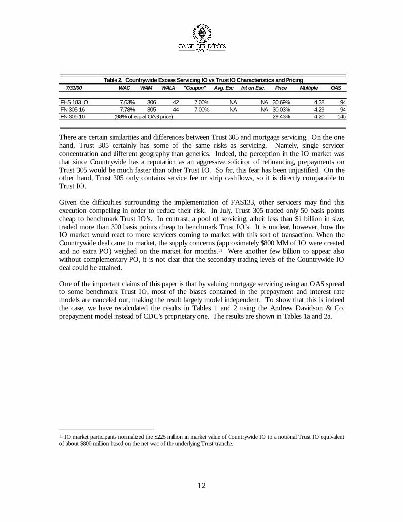
For the last several years, the main trend in the mortgage servicing market has been consolidation.Since December, 1998, the top 10 mortgage servicers have increased their market share from 34.85%to 41.62% and the total amount of mortgages serviced from $1.57 trillion to $1.99 trillion, an increaseof $420 billion in loans. The statistics are shown in Table 3. The servicers shown in Table 3generally did not come by their huge volumes purely by origination. Rather, they have been largebuyers of servicing in the open market, both in bulk and on a flow basis. The consolidation in theServicing industry is consistent with that in other industries with large fixed costs and low marginalcosts and where technologically driven platforms can be expanded relatively easily. The motivationfor servicer consolidation goes beyond cost advantages, however. Servicers are also driven by thedesire to capture “the customer for life”. The thinking goes that once a customer has a relationshipwith an institution from the mortgage process, then it will be easier to sell that customer otherproducts including credit cards, checking accounts, mutual funds, encyclopedias, etc. Once acustomer has a mortgage with an institution, then it may be more likely for that institution to capturethe next mortgage that customer takes out. These retention and ancillary income benefits havereceived a lot of attention in recent years and have been a common explanation for why servicingprices have increased as much as they have.

14

Rank Rank Name Vol Vol Mkt Sh Mkt ShMar-00 Dec-98 Mar-00 Dec-98 Mar-00 Dec-98

1 4 Chase Mortgage 324,730$ 249,661$ 6.79% 5.55%2 1 Bank of America 324,702$ 247,316$ 6.79% 5.50%3 2 Wells Fargo 286,398$ 208,599$ 5.99% 4.64%4 3 Countrywide 253,437$ 206,347$ 5.30% 4.59%5 8 Washington Mutual 165,095$ 139,608$ 3.45% 3.10%6 7 Homeside Lending 152,501$ 120,098$ 3.19% 2.67%7 5 GMAC Mortgage 150,000$ 118,797$ 3.13% 2.64%8 6 Fleet Mortgage 138,800$ 107,612$ 2.90% 2.39%9 9 First Nationwide 101,254$ 86,355$ 2.12% 1.92%10 - CitiMortgage 93,626$ 1.96%- 10 GE Capital 83,273$ 1.85%

1,990,543$ 1,567,666$ 41.62% 34.85%Source: Mortgage Servicing News, Vol. 4, No. 8, August 2000

Total

Table 3. Top 10 Servicers and Volume

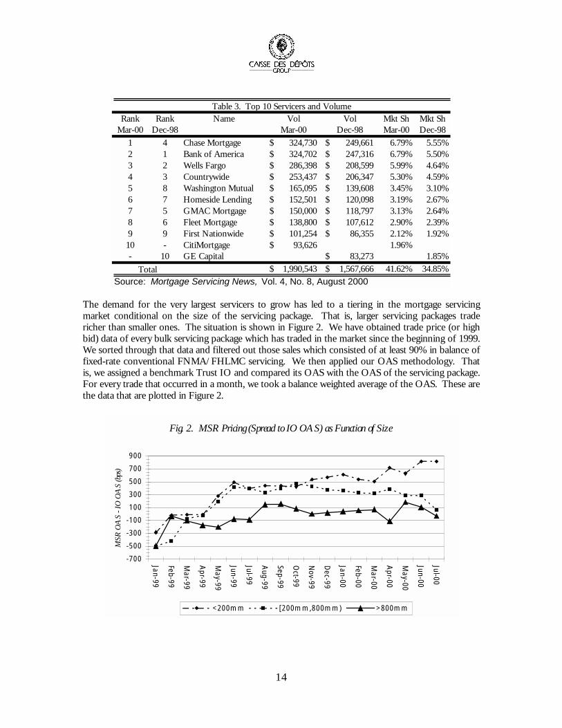
The demand for the very largest servicers to grow has led to a tiering in the mortgage servicingmarket conditional on the size of the servicing package. That is, larger servicing packages tradericher than smaller ones. The situation is shown in Figure 2. We have obtained trade price (or highbid) data of every bulk servicing package which has traded in the market since the beginning of 1999.We sorted through that data and filtered out those sales which consisted of at least 90% in balance offixed-rate conventional FNMA/FHLMC servicing. We then applied our OAS methodology. Thatis, we assigned a benchmark Trust IO and compared its OAS with the OAS of the servicing package.For every trade that occurred in a month, we took a balance weighted average of the OAS. These arethe data that are plotted in Figure 2.

Fig. 2. MSR Pricing (Spread to IO OAS) as Function of Size

-700

-500

-300

-1 00

1 00

300

500

700

900

Jan-99

Feb-99

Mar-99

Apr-99

May-99

Jun-99

Jul-99

Aug-99

Sep-99

Oct-99

Nov-99

Dec-99

Jan-00

Feb-00

Mar-00

Apr-00

May-00

Jun-00

Jul-00M

SR O

AS

- IO

OA

S (b

ps)

<200mm [200mm,800mm) >800mm

15

We segregated the servicing sales by size: sales less than $200 million in unpaid balance, thosebetween $200 million and $800 million, and those greater than $800 million. There are typically moresales per data point in the smallest size bucket than in the larger ones. There are 95 sales containedin the smallest size bucket; 46 sales contained in the medium-sized bucket; and 29 sales in the largestsized bucket. The average number of sales in each bucket is 5.0, 2.4, and 1.5, respectively. Thelargest number of sales in any month for each of the three data sets is 10, 8, and 4, respectively.

As is seen clearly in the Figure, the largest packages trade roughly flat to IO OAS; medium-sizedones trade 300-500 bps cheap to benchmark IO; and the smallest packages trade 400-600 bps cheapto IO. Note that this graph aggregates sales of different coupons because we assume thatcomparison to the relevant benchmark IO takes out most of the coupon-related effects. Weattribute this tiering to the fact that the mega-servicers’ demand for growth can best be accomplishedby buying the largest packages in the market. Purchases of smaller packages require nearly the sameamount of time and effort to close as larger packages. Although the comprehensive pre-1999 data isunavailable, CDC does have quarterly data on its own servicing portfolios in each tier, prior to thebeginning of 1999. CDC’s results indicate that the tiering began in the fall of 1998 and prior to that,servicing packages of all sizes were priced comparably on this OAS basis.

It is also interesting to note that at the beginning of the period, January 1999, all servicing traded veryrich on an OAS basis relative to IO. Over the period, all servicing cheapened dramatically, with thesmallest packages cheapening about 1000 bps and the largest ones only about 500 bps.

VI. VALUING MORTGAGE SERVICING

Using the assumptions of $10 per loan per year for the net cost to service, one-month LIBOR forthe crediting rate for P&I and T&I float, and CDC’s interest rate and prepayment models, therelative amounts of value contained in a servicing package are shown in Table 4. The servicingcomponents shown in the Table are the same as those described in Equations (2). This is thesame servicing package which has been used as an example throughout. As of 7/31/00 thispackage had a market price of 1.55%. Most of the value of servicing is contained in the servicingfee strip and in the T&I float. IO investors may be unaware that anywhere from 15%-50% ofthe value of a servicing portfolio is contained in the T&I float component. In Table 4, it isshown that 26.4% of the value of our sample servicing portolio is in the T&I float. Of course, asthe loans age and the balance on the loans pay down, the absolute and the share of value of theT&I float will increase. This is because T&I deposits continue as long as the loan is outstandingregardless of the unpaid balance on the loan. Furthermore, inflation, assumed in this case to be3% per annum, increases the property value and adds incremental value to the T&I componentover time. These effects mean that for seasoned loans, the value of the T&I float componentcan be even larger than that shown in the table. Recall, that the servicing package in thisexample has a weighted average loan age of almost 8 years. Newer servicing portfolios havecloser to 15% of their value in the T&I, while very seasoned ones may have closer to 50%.

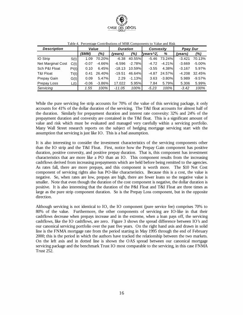
16

Description($MM) (%) (years) (%) (years^2) % (years) (%)

IO Strip 1.09 70.20% -6.38 40.55% -5.46 73.24% -3.421 70.13%Net Marginal Cost -0.07 -4.66% -6.596 -2.78% -4.72 -4.21% -3.669 -5.00%Sch P&I Float 0.10 6.45% -18.13 10.59% -3.55 4.38% -3.167 5.97%T&I Float 0.41 26.40% -19.51 46.64% -4.87 24.57% -4.208 32.45%Prepay Gain 0.09 5.47% 2.29 -1.13% 3.63 -3.80% 5.989 -9.57%Prepay Loss -0.06 -3.86% 17.022 5.95% 7.84 5.79% 5.306 5.99%Servicing 1.55 100% -11.05 100% -5.23 100% -3.42 100%

C(t)

Table 4. Percentage Contributions of MSR Components to Value and Risk Ppay Dur

S(t)

Value Duration Convexity

PI(t)TI(t)G(t)L(t)

While the pure servicing fee strip accounts for 70% of the value of this servicing package, it onlyaccounts for 41% of the dollar duration of the servicing. The T&I float accounts for almost half ofthe duration. Similarly for prepayment duration and interest rate convexity: 32% and 24% of theprepayment duration and convexity are contained in the T&I float. This is a significant amount ofvalue and risk which must be evaluated and managed very carefully within a servicing portfolio.Many Wall Street research reports on the subject of hedging mortgage servicing start with theassumption that servicing is just like IO. This is a bad assumption.

It is also interesting to consider the investment characteristics of the servicing components otherthan the IO strip and the T&I Float. First, notice how the Prepay Gain component has positiveduration, positive convexity, and positive prepay duration. That is, this component has investmentcharacteristics that are more like a PO than an IO. This component results from the increasingcashflows derived from increasing prepayments which are held before being remitted to the agencies.As rates fall, there are more prepays, and this component is worth more. The $10 Net Costcomponent of servicing rights also has PO-like characteristics. Because this is a cost, the value isnegative. So, when rates are low, prepays are high, there are fewer loans so the negative value issmaller. Note that even though the duration of the cost component is negative, the dollar duration ispositive. It is also interesting that the duration of the P&I Float and T&I Float are three times aslarge as the pure strip component duration. So is the Prepay Loss component, but in the oppositedirection.

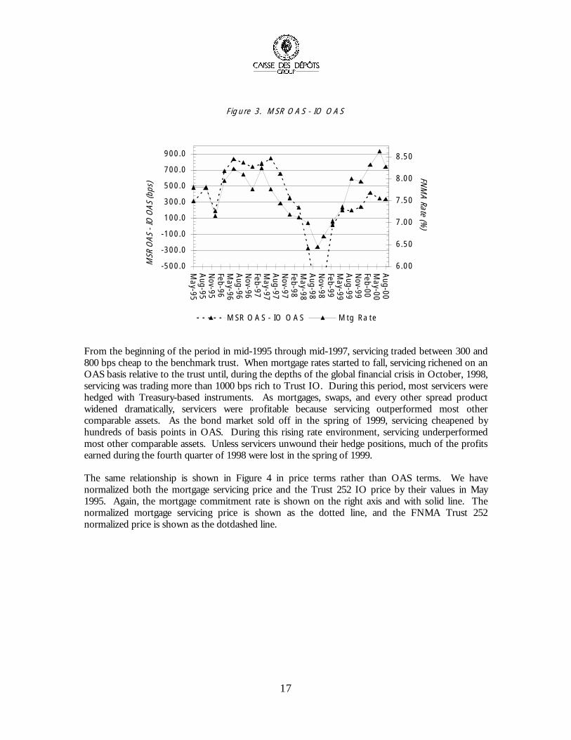
Although servicing is not identical to IO, the IO component (pure service fee) comprises 70% to80% of the value. Furthermore, the other components of servicing are IO-like in that theircashflows decrease when prepays increase and in the extreme, when a loan pays off, the servicingcashflows, like the IO cashflows, are zero. Figure 3 shows the spread difference between IO’s andour canonical servicing portfolio over the past five years. On the right hand axis and drawn in solidline is the FNMA mortgage rate from the period starting in May 1995 through the end of February2000; this is the period in which the authors have tracked the relationship between the two markets.On the left axis and in dotted line is shown the OAS spread between our canonical mortgageservicing package and the benchmark Trust IO most comparable to the servicing, in this case FNMATrust 252.

17

F ig ure 3. M SR O A S - IO O A S

-500.0

-300.0

-1 00.0

1 00.0

300.0

500.0

700.0

900.0

May-95

Aug-95

Nov-95

Feb-96M

ay-96A

ug-96N

ov-96Feb-97M

ay-97A

ug-97N

ov-97Feb-98M

ay-98A

ug-98N

ov-98Feb-99M

ay-99A

ug-99N

ov-99Feb-00M

ay-00A

ug-00

MSR

OAS

- IO

OAS

(bps

)

6.00

6.50

7.00

7.50

8.00

8.50FN

MA Rate (%

)

MSR O A S - IO O A S Mtg Ra te

From the beginning of the period in mid-1995 through mid-1997, servicing traded between 300 and800 bps cheap to the benchmark trust. When mortgage rates started to fall, servicing richened on anOAS basis relative to the trust until, during the depths of the global financial crisis in October, 1998,servicing was trading more than 1000 bps rich to Trust IO. During this period, most servicers werehedged with Treasury-based instruments. As mortgages, swaps, and every other spread productwidened dramatically, servicers were profitable because servicing outperformed most othercomparable assets. As the bond market sold off in the spring of 1999, servicing cheapened byhundreds of basis points in OAS. During this rising rate environment, servicing underperformedmost other comparable assets. Unless servicers unwound their hedge positions, much of the profitsearned during the fourth quarter of 1998 were lost in the spring of 1999.

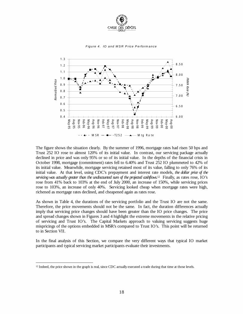
The same relationship is shown in Figure 4 in price terms rather than OAS terms. We havenormalized both the mortgage servicing price and the Trust 252 IO price by their values in May1995. Again, the mortgage commitment rate is shown on the right axis and with solid line. Thenormalized mortgage servicing price is shown as the dotted line, and the FNMA Trust 252normalized price is shown as the dotdashed line.

18

F ig u re 4 . IO a n d M S R P ric e P e rfo rm a n ce

0 .4

0 .5

0 .6

0 .7

0 .8

0 .9

1 .0

1 . 1

1 .2

1 .3

May-95

Aug-95

Nov-95

Feb-96

May-96

Aug-96

Nov-96

Feb-97

May-97

Aug-97

Nov-97

Feb-98

May-98

Aug-98

Nov-98

Feb-99

May-99

Aug-99

Nov-99

Feb-00

May-00

Aug-00

Nor

mal

ized

Pric

e

6 .0 0

6 .5 0

7 .0 0

7 .5 0

8 .0 0

8 .5 0

FNM

A Rate (%)

M S R T2 5 2 M t g R a t e

The figure shows the situation clearly. By the summer of 1996, mortgage rates had risen 50 bps andTrust 252 IO rose to almost 120% of its initial value. In contrast, our servicing package actuallydeclined in price and was only 95% or so of its initial value. In the depths of the financial crisis inOctober 1998, mortgage (commitment) rates fell to 6.40% and Trust 252 IO plummeted to 42% ofits initial value. Meanwhile, mortgage servicing retained most of its value, falling to only 76% of itsinitial value. At that level, using CDC’s prepayment and interest rate models, the dollar price of theservicing was actually greater than the undiscounted sum of the projected cashflows.12 Finally, as rates rose, IO’srose from 41% back to 103% at the end of July 2000, an increase of 150%, while servicing pricesrose to 103%, an increase of only 40%. Servicing looked cheap when mortgage rates were high,richened as mortgage rates declined, and cheapened again as rates rose.

As shown in Table 4, the durations of the servicing portfolio and the Trust IO are not the same.Therefore, the price movements should not be the same. In fact, the duration differences actuallyimply that servicing price changes should have been greater than the IO price changes. The priceand spread changes shown in Figures 3 and 4 highlight the extreme movements in the relative pricingof servicing and Trust IO’s. The Capital Markets approach to valuing servicing suggests hugemispricings of the options embedded in MSR’s compared to Trust IO’s. This point will be returnedto in Section VII.

In the final analysis of this Section, we compare the very different ways that typical IO marketparticipants and typical servicing market participants evaluate their investments.

12 Indeed, the price shown in the graph is real, since CDC actually executed a trade during that time at those levels.

19

Prepay = 150 PSA Static Static OAS OAS OAS Static a/o 3/31/00 Yield Price Spread Spread Price YieldIO Strip S(t) 9.50% 1.29% -48 174 1.21% 11.71%Net Marginal Cost C(t) 9.50% -0.09% -30 174 -0.08% 11.52%P&I Float PI(t)+G(t)+L(t) 9.50% 0.12% 723 174 0.14% 6.25%T&I Float TI(t) 9.50% 0.40% 447 174 0.45% 7.11%Total 9.50% 1.72% 174 174 1.72% 9.50%

Table 5. Static and OAS pricing for mortgage servicing

Table 5 is divided in half. The left half shows a method used by many mortgage servicers to evaluateMSR’s. Again, we have taken the canonical mortgage servicing package which has been used as anexample throughout this paper, and the components which are defined in Equations (2). At the endof March 2000, a servicing broker marked this servicing portfolio at 1.72% (at the end of July, 2000,the same broker marked it at 1.55%). Many mortgage servicers value MSR’s on a static basis. Thatis, they will assume a static discount rate, say 9.5%, a static prepayment speed, say 150 PSA, and astatic crediting rate for the P&I and T&I float, say 6.13%, which was the value of 1-month LIBOR atthat time. Assuming these parameters are applied equally across servicing components, the prices foreach component are shown in the “Static Price” column of the first sub-section. Keeping thosestatic prices constant, CDC’s model was applied to the servicing and to the benchmark Trust IO tocompute the OAS spread between the OAS of each component given the static price and the OASof the benchmark Trust IO. These spreads are shown in the “OAS Spread” column. As of the endof March, the OAS spread between the servicing and the benchmark Trust IO was 174 bps. Theinteresting result is that in the static method employed by some servicers, the service fee component,which is the largest component of servicing value, is implicitly priced 400-800 bps richer than thefloating rate components.

In the right half of Table 5, we show the servicing valuation from the capital markets point of view.Namely, at the broker-determined price of 1.72%, the OAS spread to the benchmark IO is 174 bps.If that same 174 bps spread is applied to each servicing component, the prices obtained are displayedin the “OAS Price” column. In both cases, the total price is unchanged, as is the total OAS.However, the strip price is higher in the static method and float components are priced higher in theOAS method. If the static parameters are again applied, 150 PSA, and 6.13 crediting rate, then thestatic yields which result are shown in the last column. There it is seen that the service fee is morelike 11.71% yield and the float yields are 6.25% and 7.11%. In this case, the static yields on theservice fee more resemble the static yields on Trust IO, while the float components have loweryields13.

The lower yields on the float components, however, are misleading because static yields calculated onfloating rate instruments can be either high or low depending, for example, on the shape of the yieldcurve. Indeed, when this Table was calculated, the forward one-month LIBOR rate was more like

13 Whether in yield or OAS terms, there is no reason a priori that all of the components of servicing must be priced at thesame yield or OAS. Nonetheless, we find that different pools of servicing with similar WACs and WAMs tend to trade atsimilar OAS even if the other characteristics of the servicing are somewhat different. This suggests to us that equal OASacross servicing components is not a bad assumption.

20

7.40% for several years out, with a peak at 7.60% two years forward. So the low yields reflect thefact that the static method assumes LIBOR is fixed at 6.13% rather than increasing along withforward rates. In a steep LIBOR curve environment, the static pricing method will undervalue thefloat component which will result in high OAS for those components in a dynamic pricing method.Conversely, in a dynamic pricing method, the price for the floating rate components will result in alow static yield when a lower than average crediting rate is applied. Of course, since by constructionboth the static pricing and dynamic pricing methods start with the same price for the entire package,the shape of LIBOR curve will only affect the relative value of the components within the servicingasset. When the floating rate components appear cheap, the strip component will appear rich, andvice versa. However, as the yield curve changes shape, the static yield method will require a differentyield to compute the correct price. Similarly, packages with different components of float andservice fee will need to be priced at different yields. This analysis shows some of the difficulties in astatic pricing methodology. It is true, however, that if some average forward rate is used as the staticcrediting rate instead of the spot LIBOR rate, then some of these issues can be avoided.

It is also interesting to note that the OAS spread relative to the Trust IO on the IO Strip component,)(tS , is negative. That is, when priced statically, the servicing strip is richer than the benchmark

Trust IO. It is tempting to attribute this increased value of the servicing strip to retention value orotherwise attributable to the value of the customer, and that if the customer value were valuedseparately, then this component would be priced at IO levels or wider. However, as the precedingdiscussion showed, the relative OAS valuations between the components in a static methodology isfundamentally a consequence of the shape of the LIBOR curve and its relation to the spot value.

Indeed, later in 2000, the LIBOR curve was significantly flatter and this analysis showed that thedifference in yields and OAS spreads between the strip components and the floating ratecomponents was more like 200 bps rather than 400-800 bps shown here. In fact, pricing the stripcomponent in the static method resulted in a price which appeared to be approximately the same asthat calculated in the dynamic method. Indeed, as of this writing, the difference between the spotLIBOR rate and the forward rates going out ten years is only about 10 bps.

One interesting observation in servicing pricing is that MSR’s with significant excess servicing tradeat lower multiples than the same portfolio without excess servicing. A common interpretation of thisfact is that servicers are really after customers and therefore prefer to have a smaller strip component,other things being equal. The claim is that servicers pay less for excess servicing for this reason.However, the decomposition in Table 5 shows clearly that doubling the strip component, evenpriced at the same OAS, should lower the multiple since the other components are largelyunchanged, yet they contribute significantly to the value of the servicing package.

VII . HEDGING MORTGAGE SERVICING

In order to evaluate a hedging strategy for MSR, it is important to begin with a statement of thehedge objective. Over the years, the hedge objective of most servicers has evolved from “not at all,”for pre-FAS 122 off-balance-sheet servicing, to hedging changes in MSR values determined by aLOCOM accounting methodology. Recall that the LOCOM or lower of cost or market method ofaccounting allows MSR to be marked down or up but only up to the original (or amortized) cost. Inaddition, under hedge accounting, MSR can be marked up or down to the extent of changes in thevalue of a derivative hedge. For servicers who hedge LOCOM without getting hedge accounting

21

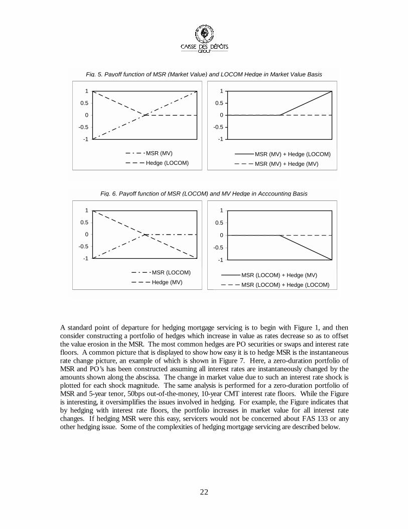
treatment, the values based on LOCOM are equivalent to the payoff function of a short put optionposition on the underlying MSR with a strike price equal to the original purchase price. Clearly, thestrategy of hedging LOCOM accounting or a short at-the-money put option position is not the sameas hedging the value of MSR for all changes in interest rates. In fact, hedging the option position iseven more complex than hedging the outright position since the option is on an underlyinginstrument which itself contains embedded (prepayment) options. In addition, the goal of hedgingthe LOCOM values is driven by accounting rules and not by the economics of the business.

The first set of figures below, Figure 5, show the payoffs of the market value hedge and the LOCOMhedge in terms of market values. The second set of figures, shown in Figure 6, shows the hedgeoutcomes in terms of accounting values. Although the market hedge theoretically shows volatility ofprofitability in accounting terms, it in fact shows no volatility in market value terms. The LOCOMhedge theoretically shows no volatility in accounting terms but in fact shows volatility in market valueterms. One is tempted to argue that the downside of the LOCOM hedge is to understate economicgains whereas the downside of the market value hedge is to show accounting losses even where nolosses exist in market value terms. Of course, even if one employed the LOCOM hedge and MSRvalues rose above cost, accounting results would show no change whereas true market values wouldshow a gain. Attempting to lock in that gain by hedging at that point would not work becausewhether MSR values rose or fell, the accounting value would not change whereas the hedge valuewould. As a result of accounting distortions, most servicers attempt to use hedge accounting rulesand thereby hedge both gains and losses in their MSR so that accounting and economics most closelyresemble each other.

In our discussion of hedging MSR below, we are approaching hedging from an economicperspective. We are not attempting to hedge LOCOM accounting rules. Rather, we are attemptingto hedge market values and will rely on a hedge accounting methodology.14 15

14 Theoretically, the techniques we describe below can be used to hedge LOCOM values by making adjustments necessaryfor hedging short put options. However, as noted above, hedging an option on an instrument which itself containsembedded prepayment options can be very complex.

15 While we do not go into the details of FAS 133, we expect to follow the requirements outlined in FAS 133 to obtainhedge accounting treatment. The difference between the FAS 133 implementation whereby the hedge “errors” passthrough the income statement and previous implementations whereby they do not has no impact on our methodology.

22

Fig. 5. Payoff function of MSR (Market Value) and LOCOM Hedge in Market Value Basis

-1

-0.5

0

0.5

1

MSR (MV)

Hedge (LOCOM)

-1

-0.5

0

0.5

1

MSR (MV) + Hedge (LOCOM)

MSR (MV) + Hedge (MV)

Fig. 6. Payoff function of MSR (LOCOM) and MV Hedge in Acccounting Basis

-1

-0.5

0

0.5

1

MSR (LOCOM)

Hedge (MV)

-1

-0.5

0

0.5

1

MSR (LOCOM) + Hedge (MV)

MSR (LOCOM) + Hedge (LOCOM)

A standard point of departure for hedging mortgage servicing is to begin with Figure 1, and thenconsider constructing a portfolio of hedges which increase in value as rates decrease so as to offsetthe value erosion in the MSR. The most common hedges are PO securities or swaps and interest ratefloors. A common picture that is displayed to show how easy it is to hedge MSR is the instantaneousrate change picture, an example of which is shown in Figure 7. Here, a zero-duration portfolio ofMSR and PO’s has been constructed assuming all interest rates are instantaneously changed by theamounts shown along the abscissa. The change in market value due to such an interest rate shock isplotted for each shock magnitude. The same analysis is performed for a zero-duration portfolio ofMSR and 5-year tenor, 50bps out-of-the-money, 10-year CMT interest rate floors. While the Figureis interesting, it oversimplifies the issues involved in hedging. For example, the Figure indicates thatby hedging with interest rate floors, the portfolio increases in market value for all interest ratechanges. If hedging MSR were this easy, servicers would not be concerned about FAS 133 or anyother hedging issue. Some of the complexities of hedging mortgage servicing are described below.

23

Fig. 7. Change in Servicing Value for Instantaneous Chanegs in Rates

-8.0-6.0-4.0-2.00.02.04.06.08.0

-200 -150 -100 -50 0 50 100 150 200

Change in Interest Rates (bps)

Cha

nge

in M

arke

t Val

ue ($

)

MSR MSR+Floor MSR+PO

In Figures 3 and 4 it was shown that the servicing-to-IO OAS spread has been very volatile over thelast several years, ranging from +700 bps to –1000 bps back to +500 bps. It can also be seenempirically that the servicing prices appear to be much less sensitive to changes in mortgage ratesthan Trust IO. If a model gives the result that the OAS consistently widen in a rally and tighten in atradeoff, then using that model for hedging will prove to be difficult.16

The first point to make about hedging servicing relates to the difference between servicing durationsand IO durations. In order to compare the price movements of servicing to IO’s, we can computethe theoretical hedge ratio between our servicing package and a Trust IO. The theoretical hedgeratio, h, is:

h = ioio

ss

io

s

PDPD

PP =

∆∆

, (3)

where Ps is the MSR price, Pio is the IO price, Ds is the MSR duration, and Dio is the IO duration.

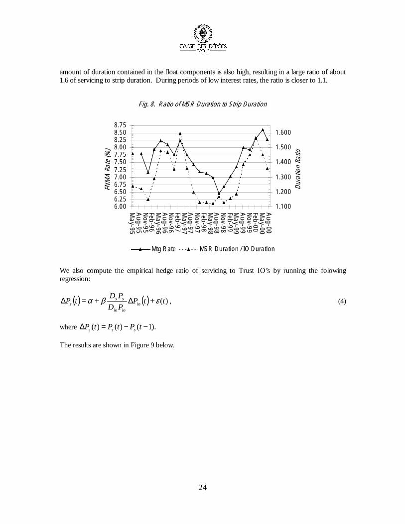
In Figure 8, we plotted the mortgage rate with a solid line. On the right axis and with the dotted lineis the ratio of our mortgage servicing portfolio model (dollar) duration to the model (dollar) duration ofjust the servicing strip portion of the asset. This is the parameter h. The result is sort of obvious.During periods when mortgage rates are high, short rates are likely high as well, and the value and

16 In practice, if the OAS widening and tightening was a deterministic function of interest rates or IO prices, then one couldcalculate a hedge strategy based on the assumption that the observed spread relationships would be maintained in thefuture. However, we observe no consistent patterns in historical spread movements.

24

amount of duration contained in the float components is also high, resulting in a large ratio of about1.6 of servicing to strip duration. During periods of low interest rates, the ratio is closer to 1.1.

F ig. 8. R atio of MSR Duration to S trip Duration

6.006.256.506.757.007.257.507.758.008.258.508.75

May-95

Aug-95

Nov-95

Feb-96M

ay-96A

ug-96N

ov-96Feb-97M

ay-97A

ug-97N

ov-97Feb-98M

ay-98A

ug-98N

ov-98Feb-99M

ay-99A

ug-99N

ov-99Feb-00M

ay-00A

ug-00

FNM

A Ra

te (%

)

1 .1 00

1 .200

1 .300

1 .400

1 .500

1 .600

Dura

tion

Ratio

Mtg R ate MS R Duration / IO Duration

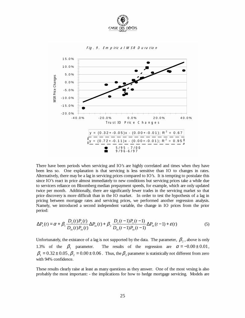
We also compute the empirical hedge ratio of servicing to Trust IO’s by running the folowingregression:

( ) ( ) )(ttPPDPDtP io

ioio

sss εβα +∆+=∆ , (4)

where ).1()()( −−=∆ tPtPtP sss

The results are shown in Figure 9 below.

25

F ig . 9 . E m p ir ic a l M S R D u r a t io n

y = ( 0 .3 2 + - 0 .0 5 ) x - ( 0 .0 0 + - 0 .0 1 ) ; R 2 = 0 .6 7

y = ( 0 .7 2 + - 0 .1 1 ) x - ( 0 .0 0 + - 0 .0 1 ) ; R 2 = 0 .9 5

- 2 0 .0 %

- 1 5 .0 %

- 1 0 .0 %

- 5 .0 %

0 .0 %

5 .0 %

1 0 .0 %

1 5 .0 %

- 4 0 .0 % - 2 0 .0 % 0 .0 % 2 0 .0 % 4 0 .0 %T r u s t IO P r ic e C h a n g e s

MSR

Pric

e Ch

ange

s

5 / 9 5 - 7 / 0 09 / 9 6 - 6 / 9 7

There have been periods when servicing and IO’s are highly correlated and times when they havebeen less so. One explanation is that servicing is less sensitive than IO to changes in rates.Alternatively, there may be a lag in servicing prices compared to IO’s. It is tempting to postulate thissince IO’s react in price almost immediately to new conditions but servicing prices take a while dueto servicers reliance on Bloomberg median prepayment speeds, for example, which are only updatedtwice per month. Additionally, there are significantly fewer trades in the servicing market so thatprice discovery is more difficult than in the IO market. In order to test the hypothesis of a lag inpricing between mortgage rates and servicing prices, we performed another regression analysis.Namely, we introduced a second independent variable, the change in IO prices from the priorperiod:

)()1()1()1()1()1()(

)()()()()( 21 ttP

tPtDtPtDtP

tPtDtPtDtP io

ioio

ssio

ioio

sss εββα +−∆

−−−−+∆+=∆ (5)

Unfortunately, the existance of a lag is not supported by the data. The parameter, 2β , above is only1.3% of the 1β parameter. The results of the regression are 01.000.0 ±−=α ,

05.032.01 ±=β , 06.000.02 ±=β . Thus, the 2β parameter is statistically not different from zerowith 94% confidence.

These results clearly raise at least as many questions as they answer. One of the most vexing is alsoprobably the most important: - the implications for how to hedge mortgage servicing. Models are

26

useful for many relative value questions and we believe that by spreading to Trust IO much of themodel sensitivity is reduced. However, when thinking about hedging, one has to be more careful.

In the IO market, it often happens that a particular interest rate model and prepayment model give aduration for Trust IO which is different from how the market prices are moving with respect tointerest rates. A hedger in this situation has two choices: he can continue to use his model durationin the belief that over the long haul the market-implied duration will converge to the model durationand he may realize significant p&l volatility in the interim, or he can throw out his model and hedgeto market-implied or market-consensus durations on the IO, reducing the p&l volatility but makinghim appear unhedged on a model basis. In such a case when the model duration diverges from themarket-implied duration, it is still possible to hedge perfectly by buying a PO and selling MBScollateral. However, this is only possible because of the existence of the complement of the IO: thePO. Indeed, some participants in the securities markets argue that this is a reason why even well-structured PAC IO must trade behind Trusts, because of the lack of the complement. In the case ofmortgage servicing, the situation is even worse since not only is there no such thing as thecomplement to the T&I float. Moreover, the T&I float component itself does not trade separately inthe marketplace. If a particular model is giving the “wrong” duration on Trust IO, then that must bealso “wrong” for the float, but the trader or portfolio manager will not have any idea how to correctfor the errors or how to find the market-implied duration for these components.

Furthermore, even if some strategy for hedging the floating rate components is determined, there arestill risks. For instance, the most natural hedge for servicing is PO. That is to say, a PO is the mostnatural hedge from an economic perspective in that it will reduce the prepayment risk, even though itmay not reduce p&l volatility as seen in Figure 4. Other risks include the fact that by simply buyingPO there is also the so-called “combo premium”. The combo premium is the difference betweenthe sum of the Trust IO and PO prices and the collateral price. In general, the combo premium isbounded from below by zero and can be substantially positive. This reflects the fact that differentmarket participants can have different prepayment views and can lever those views in either IO orPO independently. In Table 6 is shown the value of certain combo premiums from 12/97 through6/00, in 32nd’s of a point.

Trust Coupon WAM 12/97 03/98 06/98 09/98 12/98 03/99 06/99 09/99 12/99 03/00 06/00T249 6.5 269 33 31 19 5 9 13 23 42 51 40 40S192 6.5 326 n/a 5 6 (2) (1) 2 4 10 19 17 17T240 7.0 266 n/a 17 12 1 1 3 (3) 28 30 28 28S183 7.0 313 16 12 16 (1) 0 3 1 7 10 20 20T252 7.5 265 30 36 17 (0) (0) 7 6 19 18 22 22T284 7.5 318 15 22 11 (0) (0) 7 2 11 19 19 19

Table 6. Combination premiums of IO/PO Trusts (in 32nd's)

As can be seen clearly in the Table, these premiums can range from a few ticks for new collateral toas much as 1 ½ points for seasoned. Much of the large premiums simply reflect the value ofseasoned collateral over new collateral. However, the value of seasoned collateral over new did notpersist during the financial crisis in the fall of 1998 when combo premiums on all collateral seasonedand new alike vanished.

27

What the numbers in Table 6 say is that a servicer who buys servicing and hedges with PO, or an IObuyer who buys IO and hedges with PO can easily lock in a certain amount losses by buying the POand selling collateral, if he does everything right.

Servicers often talk about the “Natural” hedge: namely, production of new servicing. Originationvolumes increase in periods of low interest rates and decrease in periods of high interest rates,partially offsetting the value changes in the MSR on the balance sheet. From a hedging perspective, aservicer can account for this natural hedge by determining how his originations will change withinterest rates and valuing the change in those originations accordingly. This hedge will never cover100% of the change in MSR value because even if a servicer retained 100% of his MSR portfolio in aperiod of high prepayments, there is a cost associated with making those originations so that theservicer is in effect buying the new servicing (at the cost of originating the new loan). If the cost tooriginate were equal to the market value of the servicing, then the natural hedge would not be ahedge at all. It would merely be a method of acquiring replacement servicing at the cost in themarket. However, if the cost to originate were lower than the market value then the natural hedgecould be an important and significant component of servicing values and hedge strategies.Nonetheless, the loss of value on the prepaid amount will typically be greater than the incrementalservicing value acquired (by the cost of origination). Typically, the cost to originate a new loan costssomewhere in the neighborhood of 75-100 bps. A “streamlined” loan probably costs somewherearound 50-75 bps. In today’s market, the average market value of new servicing is probably 1.50,around 6 multiple. So, in recapturing loans which prepay, the servicer can hope to only lose half hisinvestment in those loans. Unfortunately, the recapture rate of servicers is only around 10% forprepaying loans. That is, servicers typically lose 95% of their investment in loans which prepay.Even if the recapture rate were as high as 30%, which is a goal of most servicers, the loss would stillbe 85% of investment. Five to fifteen percent of price is not negligible, but neither is it important.Nevertheless, one can take account of the amount of prepaid servicing retained in calculating thevalue and hedge ratio using the techniques we describe in the paper. Although we have neglectedthis component in the analysis presented previously, we now describe how a simple model of theretention component affects the results in this paper.

We have chosen to focus on a servicing portfolio which traded in the marketplace on 11 October2000. This package had an unpaid principal balance of $3.14 Billion and a 7.50% WAC and a 233month WAM. The net service fee was a weighted average 39.6 bps. The traded price was 1.97%.Using the methodology described in Table 1, the OAS spread to the benchmark Trust IO was –53bps. (Note that if we price this portfolio statically, using our assumption of $10 net marginal cost,then the static yield is 10.56%.) This spread is consistent with where other larger sized packages aretrading in the market at this time.

In order to get a handle on the value of the retention, it is necessary to consider 2 variables: theretention rate and the difference between the origination cost and the current market value. Wemake the assumption that whatever loans are retained are immediately sold in the marketplace on aflow basis and the difference between origination cost and current market value is realized in thatperiod. In this way, the balance of the portfolio declines just as it does without including thiscomponent, but there is an extra cashflow amount. In Figure 10 the spread between the MSR OASand the IO OAS are plotted as a function of the retention rate for four different origination costs. Inparticular, the solid line assumes that the difference between the origination cost and the currentmarket value (at any period) is 25 bps; the dashed line assumes this difference is 50 bps; the dottedline 75 bps; and the dot-dashed line assumes that this difference is 100 bps.

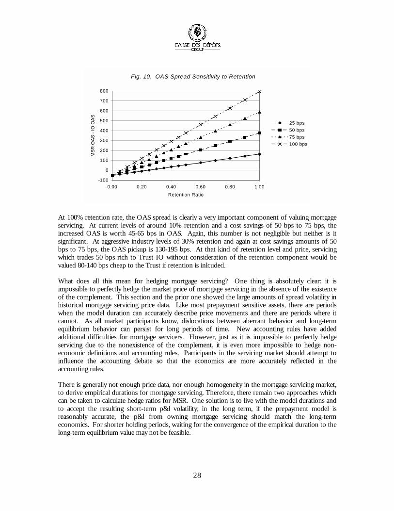
28

Fig. 10. OAS Spread Sensitivity to Retention

-100

0

100

200

300

400

500

600

700

800

0.00 0.20 0.40 0.60 0.80 1.00Retention Ratio

MSR

OAS

- IO

OAS

25 bps50 bps75 bps100 bps

At 100% retention rate, the OAS spread is clearly a very important component of valuing mortgageservicing. At current levels of around 10% retention and a cost savings of 50 bps to 75 bps, theincreased OAS is worth 45-65 bps in OAS. Again, this number is not negligible but neither is itsignificant. At aggressive industry levels of 30% retention and again at cost savings amounts of 50bps to 75 bps, the OAS pickup is 130-195 bps. At that kind of retention level and price, servicingwhich trades 50 bps rich to Trust IO without consideration of the retention component would bevalued 80-140 bps cheap to the Trust if retention is inlcuded.

What does all this mean for hedging mortgage servicing? One thing is absolutely clear: it isimpossible to perfectly hedge the market price of mortgage servicing in the absence of the existenceof the complement. This section and the prior one showed the large amounts of spread volatility inhistorical mortgage servicing price data. Like most prepayment sensitive assets, there are periodswhen the model duration can accurately describe price movements and there are periods where itcannot. As all market participants know, dislocations between aberrant behavior and long-termequilibrium behavior can persist for long periods of time. New accounting rules have addedadditional difficulties for mortgage servicers. However, just as it is impossible to perfectly hedgeservicing due to the nonexistence of the complement, it is even more impossible to hedge non-economic definitions and accounting rules. Participants in the servicing market should attempt toinfluence the accounting debate so that the economics are more accurately reflected in theaccounting rules.

There is generally not enough price data, nor enough homogeneity in the mortgage servicing market,to derive empirical durations for mortgage servicing. Therefore, there remain two approaches whichcan be taken to calculate hedge ratios for MSR. One solution is to live with the model durations andto accept the resulting short-term p&l volatility; in the long term, if the prepayment model isreasonably accurate, the p&l from owning mortgage servicing should match the long-termeconomics. For shorter holding periods, waiting for the convergence of the empirical duration to thelong-term equilibrium value may not be feasible.

29

CDC’s approach to hedging MSR is to make adjustments to model-derived IO hedge ratios andpartial durations based on certain empirical results and to apply these same adjustments to the modelderived hedge ratios and partial durations for MSR. For example, if Trust IO’s are trading to muchmore negative durations than models would indicate, CDC might shift the elbow of the prepaymentcurve by an amount necessary to obtain the empirical trading duration of the Trust IO, and then usethat same shifted model to compute the duration of mortgage servicing.

It should be stressed that the discussion in this section refers to the price sensitivity of MSR to anymarket parameter. For simplicity, we have focused on interest rates and mortgage rates. Specifically,in periods of low prepayment volatility then the methods described in this section regarding thehedge ratios of IO’s and MSR’s can be usefully applied, whether the hedge instruments are PO’s,Treasuries, interest-rate swaps, floors, or whatever. Now, it may be true that Treasuries will exhibitlarger errors in hedging MSR than, say, PO’s will, but that is a question not of hedge ratio or durationbut of basis risk.

It is also true that the analysis in this section can be applied to the hedging of prepayment duration.Recall that over the period September 1998 through March 1999, the mortgage universe experiencedthe most massive prepayment wave ever, and it reverberated throughout the sector until well into thewinter months of 1999. Unless prepayment-sensitive hedges were employed, then hedges during thisperiod proved inadequate in specifically hedging against prepayment risk. Because there is a limitedsupply of hedge instruments which have non-vanishing prepayment duration, it is impossible forlarger servicers to hedge out their sensitivity to prepayments. As a result, prepayments still remain,and will always remain, a significant risk of owning mortgage servicing.

VIII . SUMMARY AND CONCLUSIONS

In this paper, we have shared some of the most interesting results which we have observed intracking the relationships between the IO securities markets and the mortgage servicing rightsmarkets over the last five years. In our view, the most interesting result is the massive servicing-to-IO spread tightening and widening, on the order of more than a thousand basis points, which hasoccurred over that time. As a result, hedging mortgage servicing remains extremely difficult. In fact,even assuming that the market sensitivities to price can be completely hedged out by using anapproach like CDC’s described in this paper, the spread volatility experienced by MSR dominates thep&l over short time frames.

Nevertheless, hedging mortgage servicing is still the focus of much attention due to the imminentadoption of FAS133 and the p&l volatility which will flow through to earnings. This is in contrast tothe current situation where hedge “ineffectiveness” is offset by gains or losses in the hedgeinstruments, subject to hedge accounting rules. For larger companies which have earnings in therange of $500MM-$1Billion per quarter, the p&l volatility is huge. In the Introduction to this paper,it was pointed out that for 100 bps change in the servicing-to-IO spread, a servicer with $3 Billion -$4 Billion in assets would experience $100 MM - $140 MM in p&l volatility. Calculating from thesame data as in Figure 3, the standard deviation of servicing-to-IO OAS spread over the past fiveyears is about 450 bps; the p&l volatility experienced by large mortgage servicers can be very large,indeed.

30

Servicers face many difficult hedging decisions. In the Trust IO/PO markets, it is possible to hedgein a model independent fashion by buying the complement and selling the underlying collateral.Since the complement for servicing does not exist, a MSR hedger must decide how to implement ahedging strategy. In the securities markets, when model IO durations diverge from empirical IOdurations, a trader will most often adjust his duration to the empirical. CDC’s approach to hedgingmortgage servicing has been to treat servicing in a similar manner. Namely, in the case when themodel IO duration is different from the empirical, the prepayment model can be adjusted to obtainmarket implid hedge ratios, and that adjusted model can be applied to the MSR. While thismethodology will not produce optimal results in the case where the empirical IO duration (andempirical MSR duration) converges to the equilibrium model durations, it will produce better resultsin the non-convergence case. This methodology certainly requires a regular monitoring andrecalibration of the adjusted prepayment model.

The precise nature of the adjustment made to the prepayment model in such circumstances is alsosubjective. For instance, if prepayments in the model seem to be running too slow, then they can besped up by increasing the turnover speed, increasing the peak speed attainable in periods of low rates,shifting the elbow thereby reducing refinancing incentive, increasing the so-called media-effect,increasing the steepness of the prepayment curve, etc. Other adjustments might include linking pricechanges to changes in implied volatility or the shape of the yield curve.

We believe that all of the current focus on hedging mortgage servicing will most likely have asmoothing effect on servicing-to-IO spreads. As servicing market participants focus more and moreon hedging their risks, this will increasingly mean using more prepayment sensitive hedgeinstruments, e.g. PO. As the servicers start to pay more attention to the IO/PO market and shift inand out of the PO hedges depending on relative richness or cheapness compared with other hedgealternatives, it can be argued that the price of servicing will eventually move in a more correlatedfashion to the price of IO than has been observed historically.

The smaller and medium-sized servicers are able to hedge their risks by buying prepayment sensitivesecurities and can opportunistically buy mortgage servicing when servicing-to-IO spreads are wideand sell when those spreads are tight.

The larger mortgage servicers are in a different situation. Not only are they unable to hedge theirrisks completely due to the lack of enough prepayment duration in the securities markets, but theyare also unable to buy and sell servicing in the sizes needed to be meaningful. The big servicers arein the business to stay. The adoption of FAS133 and the attendant p&l volatility caused by massiveservicing-to-IO spread movements will cause the large mortgage servicers to experience large p&lswings. The mega-servicers must be prepared to accept these p&l swings as the cost of being in theservicing business. To the extent that those companies or their shareholders are unable or unwillingto accept such large p&l swings in their earnings at current MSR pricing levels, then MSR prices willdecline to reflect the risks of owning servicing. We suspect that after some number of servicers takea $100 MM or more loss due to servicing hedging mismatch, the MSR repricing will not be farbehind. This repricing itself will be painful to many of the large servicers who have their servicingmarked at current market levels. The ultimate clearing level for mortgage servicing is, of course,unknown at this time. However, we feel that the risks are significant enough that we would not besurprised to find that the equilibrium price of servicing is a multiple or more lower than it is today.

31

IX. ACKNOWLEDGEMENTS

The ideas presented in this paper are the result of many discussions the authors have had over theyears with each other and with other people. The authors wish to thank Don Brownstein, EricRaiten, Jacques Rolfo, Ramine Rouhani, and Cathy Wang for many useful discussions. We also wishto thank Andrew Davidson for providing a version of his prepayment model which is also used inthis paper.