987 measurement of velocity and vorticity fields in j the ... · pdf filemeasurement of...

NASA i 1, 1 Technical

Paper 2780 1

I

I 987

National Aeronautics and Space Administration

Scientific and Technical Information Division

Measurement of Velocity J

and Vorticity Fields in the Wake of an Airfoil in Periodic Pitching Motion

Earl R. Booth, Jr. Langley Research Center Hampton, Virginia

https://ntrs.nasa.gov/search.jsp?R=19880003620 2018-04-17T00:45:21+00:00Z

Abstract The velocity field created by the wake of an air-

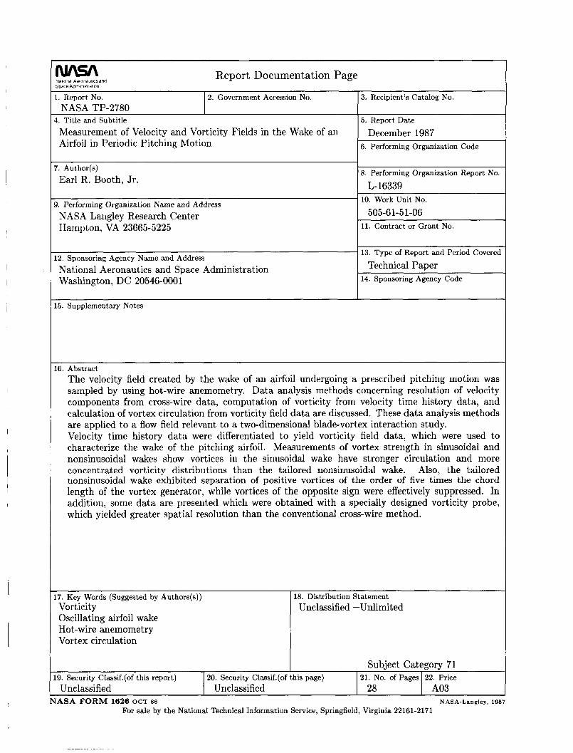
foil undergoing a prescribed pitching motion was sampled by using hot-wire anemometry. Data analysis methods concerning resolution of velocity components from cross-wire data, computation of vorticity from velocity time history data, and calculation of vortex circulation from vorticity field data are discussed. These data analysis methods are applied to a flow field relevant to a two-dimensional blade-vortex interaction study.

Velocity time history data were differentiated to yield vorticity field data, which were used to characterize the wake of the pitching airfoil. Measure- ments of vortex strength in sinusoidal and nonsinusoidal wakes show vortices in the sinusoidal wake have stronger circulation and more concentrated vorticity distributions than the tailored nonsinusoidal wake. Also, the tailored nonsinusoidal wake exhibited separation of positive vortices of the order of five times the chord length of the vortex generator, while vortices of the opposite sign were effectively suppressed. In addition, some data are presented which were obtained with a specially designed vorticity probe, which yielded greater spatial resolution than the conventional cross-wire method.

1 t

1

Introduction Blade-vortex interaction (BVI) is the source of a

major component of helicopter noise. To study the fundamental physics of BVI, a research program designed to explore two-dimensional blade-vortex interaction (2-D BVI) was initiated at NASA Langley Research Center. The key to simulation of 2-D BVI is the generation of two-dimensional vortex flow fields. The method of generation chosen was oscillation of an airfoil in pitch such that the vorticity shed from the airfoil into the wake organized into sufficiently concentrated transverse vortices. The method of vortex generation has been reported along with an an- alytical method for determining the resulting wake structure (ref. l), but the actual flow field had not been measured directly, a serious shortcoming. This study was designed to make flow field measurements in the vortex flow field to complement the 2-D BVI data (refs. 1, 2, and 3). An additional objective of this investigation was to evaluate a prototype vorticity probe in a research environment.

The velocity field created by the wake of an airfoil undergoing a prescribed pitching motion was sampled by using hot-wire anemometry. The velocity data were differentiated to yield vorticity field data. The vorticity data were used to characterize the wake of the pitching airfoil for two conditions relevant

to a 2-D BVI study. In addition, some data were obtained with a specially designed vorticity probe, which yielded greater spatial resolution than the conventional cross-wire method.

Symbols I

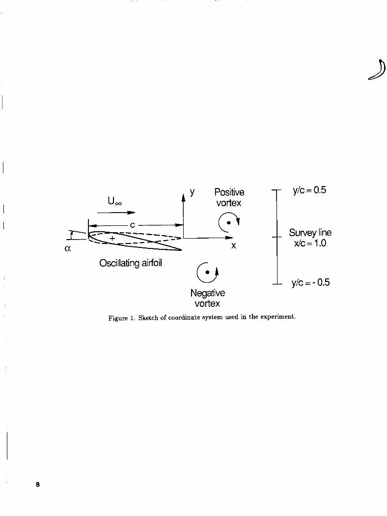
The coordinate system used in this study is presented in figure 1.

A

A1

B

B1

d

E

c

f i k m n

Q R S

t U

u, U

V

Vn

Vl, 02

X

Y

z

Q

r 6

P

constant calibration constant constant calibration constant chord length of vortex generator, 6.0 in.

hot-wire diameter hot-wire bridge voltage, V frequency of airfoil oscillation, Hz hot-wire current, A reduced frequency, 7r f c/U, integer

calibration constant heat lost from hot wire to flow resistance, R reciprocal of sample rate, sec time, sec total velocity in the z-direction, U, + u, ft/sec

free-stream velocity, ft/sec perturbation velocity in the z-direction, ft/sec

perturbation velocity in the y-direction, ft/sec

velocity normal to hot wire, ft/sec velocity normal to wire 1 and wire 2, respectively

downstream direction direction perpendicular to the free- stream velocity vector

direction normal to x-y plane airfoil angle of attack, deg

circulation of vortex, ft2/sec flow direction angle, deg viscosity, slug/ft-sec

P density, slug/ft3 w component of vorticity vector in the z-

direction, l/sec

Experimental Methodology

Experimental Setup The experiment was performed in the Langley

Aircraft Noise Reduction Laboratory using the Quiet Flow Facility as a low-speed, low-turbulence wind tunnel. A two-dimensional test section was formed by installing two side plates to the edges of a 1.0- by 1.5-ft nozzle, which was itself mounted to the 4-ft-diameter low-speed duct of the facility. The laboratory is described in more detail in reference 4.

An oscillating airfoil device was installed between the side plates downstream of the nozzle exit plane. A 6-in. chord, NACA 0012 airfoil model was driven in pitch about the quarter-chord station in pitch schedules determined by a motor-cam-transmission assem- bly. The pitch schedules, determined by inserting the proper cam, consisted of a sinusoidal oscillation and a tailored oscillation, both with a 10" amplitude. The tailored-oscillation pitch schedule consisted of a sinusoidal-like sweep from minimum incidence to maximum incidence for the first 20 percent of the cycle, with a linear return sweep making up the re- maining 80 percent of the cycle. Oscillation rate was set by motor speed, which was continuously variable. The two wakes of interest in this study were produced by oscillating the airfoil sinusoidally at 30 Hz, referred to henceforth as the sinusoidal wake, and by oscillating the airfoil by the tailored pitch schedule at 6 Hz, referred to as the tailored wake. An opti- cal encoder in the motor system provided the time reference signal for conditional sampling.

Velocity in the two-dimensional test section was monitored with a Pitot-static probe at the nozzle exit plane. Since the wake produced by the oscillating airfoil is a function of reduced frequency I C , the desired test velocity was determined by the oscillation rate and was 20 ft/sec, as measured at the nozzle exit. This flow rate actually produced a mean velocity of 15 ft/sec at the flow survey station. Because of the low test velocity and the open circuit wind-tunnel facility, variation in outside wind conditions produced significant variation of test section velocity. As a result, data were taken conditional to both the flow velocity and the time reference signal.

Description of Hot-wire Probes Data were acquired with a constant temperature

hot-wire anemometer connected directly to a four- channel analog-to-digital A/D unit. The data were

conditionally sampled by using the flow velocity data to arm the system and the time reference encoder signal to trigger the A/D unit, which then sampled the hot-wire bridge voltage at a given sample rate for a specified length of time. To provide data records covering more than one oscillation period, the sampling rate for the sinusoidal wake was 10000 samples/sec covering a time of 0.15 sec. Similarly, for the tailored wake, the sampling rate was 5000 samples/sec and the record length was 0.30 sec. Both conditions yielded a data record 1500 points long.

Two types of hot-wire probes were employed in the current study. Most of the data were obtained with a commercially produced cross-wire probe. Some data were obtained with a prototype vorticity probe.

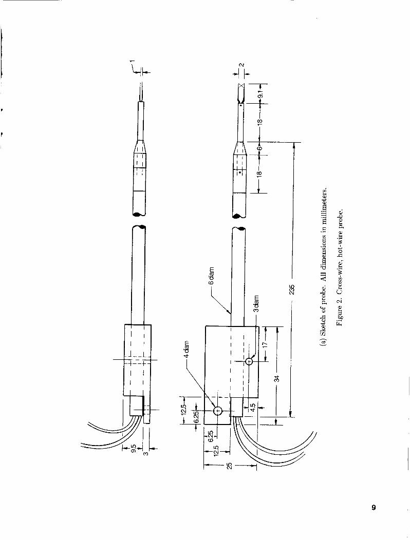
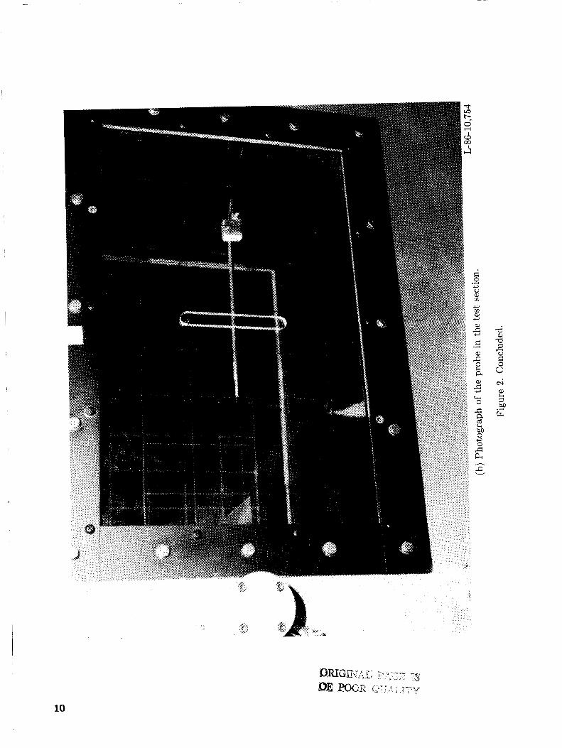
Cross-wire probe. Several commercially obtained cross-wire probes were used to survey the flow field in the wake downstream of the oscillating airfoil. The probes were Dantec 55P51 probes described in reference 5. The cross-wire probe was used to measure velocity and flow direction in the x-y plane as functions of spatial position and time. A sketch of the probe and a photograph of the probe in the test section are presented as figure 2.

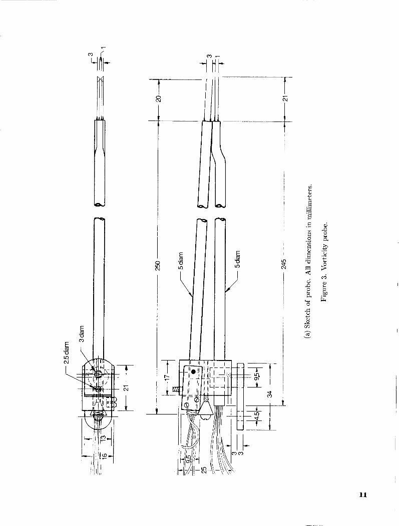
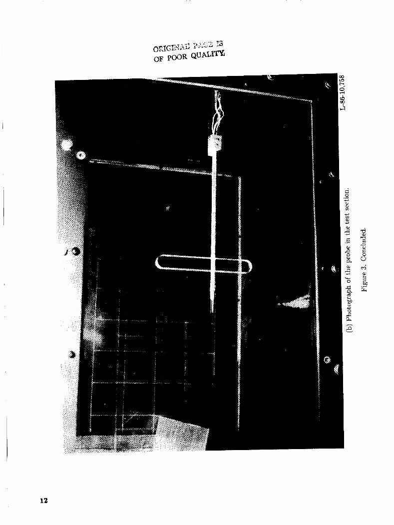
Vorticity probe. As covered in the data analysis section below, the data obtained with the cross- wire probe were used to compute the vorticity field that characterizes the wake. However, this method required time-synchronized velocity time histories at two closely spaced points to perform the data reduction; thus spatial resolution of the vorticity calculation is determined by both the sample rate and the spatial distance between data points. A more complicated probe, designed to improve spatial resolution of the vorticity measurement as well as to eliminate the need for correlation between data samples from two points, was employed to measure the tailored wake. Data obtained with the vorticity probe are compared with data from the cross-wire probe. A full description of the vorticity probe is contained in reference 6; a sketch of the probe and a photograph of the probe in the test section are presented as figure 3.

Description of Experimental Process

Two basic types of flow survey were accomplished in the experiment. First, data were obtained at a given x, y location in various z planes to determine to what extent the wake produced by the oscillating airfoil was two-dimensional. Second, data were obtained at a given 2, z location at a series of y stations to yield the velocity field crossing the survey

2

r line as a function of time. The hot-wire probe was traversed mechanically across a selected survey line at the z/c = 1.0 station. Data were obtained for y/c values from -0.5 to 0.5 in increments of 0.033~. These data were used to compute the vorticity field as a function of y/c and time. The bulk of the data reported here is from the second type of flow survey.

Data Analysis Data analysis involved three main processes: en-

semble averaging of the hot-wire bridge voltage signals, conversion of hot-wire bridge voltage time histories into velocity time histories, and calculation of vorticity from the velocity time histories.

i I

Ensemble Averaging of Hot-wire Signals The raw data were in the form of bridge voltage

from the hot-wire anemometer at a time referenced to airfoil oscillation for a series of data points. Since this was a real flow, some variation due to turbulence, variation of test section velocity, and other factors combined to make each data sample unique and only partially representative of the flow for which measurement was desired. As a result, it was necessary to average the conditionally sampled data to produce a data sample representing an average flow. This process, known as ensemble averaging, is described in reference 7 along with methods to estimate the uncertainty in the data.

Unaveraged time history data were collected and examined to determine what percentage of the hot- wire signal was random and to compute the number of averages needed for a given uncertainty level. The time history data were then averaged and compared with independent averaged data to confirm data repeatability. It was determined that 20 data records could be averaged into a data record with good repeatability characteristics. The repeatability of the data is vital to perform the vorticity calculation, as differentiation magnifies the randomness present in sampled data, particularly the cross-wire data, where independent samples are cross differentiated.

Resolution Into Velocity Data Hot-wire bridge voltage data were converted into

velocity data by using calibration coefficients obtained during calibration runs. A probe was removed from the experimental apparatus and placed in a variable-speed flow. The output bridge voltage was then curve fitted to Reynolds number based on the wire diameter. Parameters describing the resulting curve were used as calibration coefficients. Although day-to-day changes in the calibration coefficients are small, indicated velocity is very sensitive to small

changes in calibration coefficients. As a result, the calibration process was performed daily to minimize error in velocity data.

The calibration was based on King's Law. This approach assumes that, although the hot wire actually can exchange heat with the test medium through radiation, conduction, and convection, the heat lost because of conduction and radiation is negligible. In the steady state, the amount of heat Q lost from the hot wire to the flow (through convection) is

Q = i2R (1) This equation can be expressed in terms of non-

dimensional Nusselt number Nu and Reynolds number Re as

NU = A + B& where A and B are found from calibration (ref. 8). Since Nu is proportional to the square of the bridge voltage, this equation can be expressed as

(3) To allow another degree of freedom in the curve

fit, the power to which the Reynolds number is raised is expressed as l /n , with the understanding that n should be close to 2. Thus, the Reynolds number can be expressed as a function of bridge voltage by the relation

(4)

The data were thus converted from bridge voltage to Reynolds number by the above relation. Velocity was obtained from the Reynolds number by using the relation

(5)

with measured density for p, standard values for p, and the hot-wire diameter for d.

At this point, the data were in the form of velocity normal to the hot wire as a function of time. To convert from this coordinate system to the experimental frame of reference, a further calibration was performed. At a constant velocity, the hot wire was rotated from an angle of 6' = -90" to 6' = 90" in 2" increments, where the probe was aligned with the flow at 6' = 0'. The ratio of the normal velocities from wires 1 and 2 was used as a calibration curve for flow direction. This curve exhibits a maxima near 6' = 45" and a minima near 6' = -45", so the curve between these extrema was used to compute flow direction. In addition, a flow magnitude correction was computed based on the square root of the sum of the squares

3

of V I and v2 divided by the t,rue velocity. With these two curves, the velocity data were converted from v1 and v2 to U and v as functions of time. The constant mean velocity, 15 ft/sec, was subtracted from U as the free-stream velocity to yield u.

Calculation of Vorticity and Circulation The main purpose of this flow survey was to

determine the circulation of the vortices in the wake of an oscillating airfoil. In a two-dimensional flow, only one component of vorticity is present. The purpose of this section is to explain how vorticity at a point is computed with the velocity time histories and how these vorticity data are used to calculate the circulation of vortices in the airfoil wake.

In the experiment, velocity time history data of the form

(6 ) u = U(Y,t) v = V(Y,t)

were obtained for a series of points spatially separated by a constant Ay. Obviously then, Ay is one length scale defining spatial resolution of the velocity measurement. In two-dimensional flow, vorticity is given by

(7) a v a u ax a y

u = - - -

Evaluation of au/ay is straightforward; however, evaluation of av/ax requires a bit of manipulation.

Consider a two-dimensional vortex traveling through the test section at a velocity U,. Fixed inside the test section is a cross-wire probe measuring the velocity sum of U , and perturbation velocities induced by the vortex, u and v. As the vortex approaches the probe at time t i , the probe measures velocities U,+u(tl) and v(t1). Some small At later, at t 2 , the probe measures velocities U , + u(t2) and v(t2). In a probe-fixed coordinate system, then

Unfortunately, this is not the d v / d x appropriate for calculation of vorticity in the vortex. Measuring vorticity distribution in a vortex, as opposed to measuring vorticity flux at the probe, requires a vortex-fixed coordinate system. Consider, in such a reference frame, that the cross-wire probe appears to fly through the vortex at a velocity -Urn. At time t l , the probe measures U, + u( t1) and v(t1) as before. Similarly, at time t 2 , the probe measures U,+u(t2) and 4 2 ) . This time, however, the length scale is the

distance the probe appears to have moved, from the vortex’s perspective, -U,At. Thus, in the vortex- fixed reference system

4 t 2 ) - v(t1) (9) I vortex fixed = lim ax ~ t - 0 -U,At

This is the appropriate derivative for vorticity calculation, and the appropriate length scale for resolution of the vorticity measurement is some multiple of U,At.

A space-centered first approximation of the vorticity is given by

v(y, t - ms) - v(y, t + ms) 2msU, 4 Y , t ) =

where m is chosen so that

m = Integer - (11) [S%l

so that the two length scales are approximately equal. For the data from the tailored oscillation, s = 0.0002 sec/point, U, = 15 ft/sec, and Ay = 0.20/12 ft. Thus, m = 6 for this case.

An implication of this method is that vorticity cannot be computed for the first six data points or the last six data points of the data record. In this case, this is not a major concern, since the data record length exceeds one oscillation period. Also, this method is valid only if the data are sampled at a rate greater than U,/Ay.

The above method applies to the cross-wire data. The vorticity probe uses four hot-wire elements: two crossed wires and two parallel wires normal to the flow direction. Thus, the Ay used for the vorticity probe is the distance between the parallel wires, hence the length scale for the measurement is much less. As a result, a smaller sample area is considered in the vorticity calculation with m (from eq. (11)) equal to one. Thus, vorticity is measured with greater spatial resolution.

With the present data, there are particularly large concentrations of vorticity indicative of the major vortex filaments in the wake. The purpose of this investigation was to determine the strength of these vortex filaments.

Once the vorticity is known for a given range of y/c and time, it is possible to integrate the vorticity over an “area” to compute the circulation acting in

4

that area. The method used is described in reference 9. By using the relation below, the vorticity is integrated over a surface to produce the circulation.

r = - / / w . n d S (12)

where S is the surface over which the integration The double

integral was rewritten as a double summation, the differential area was computed by using the sampling rate, free-stream velocity, and distance between survey points, and a relatively simple computer routine was written to perform the integration.

1 takes place, in this case the z-y plane.

Results The data will be discussed in three parts: assess-

ment of flow two-dimensionality, results from the sinusoidal wake, and results from the tailored wake.

Flow Two-Dimensionality

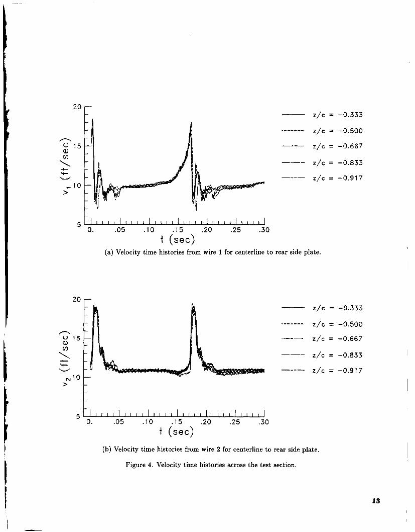
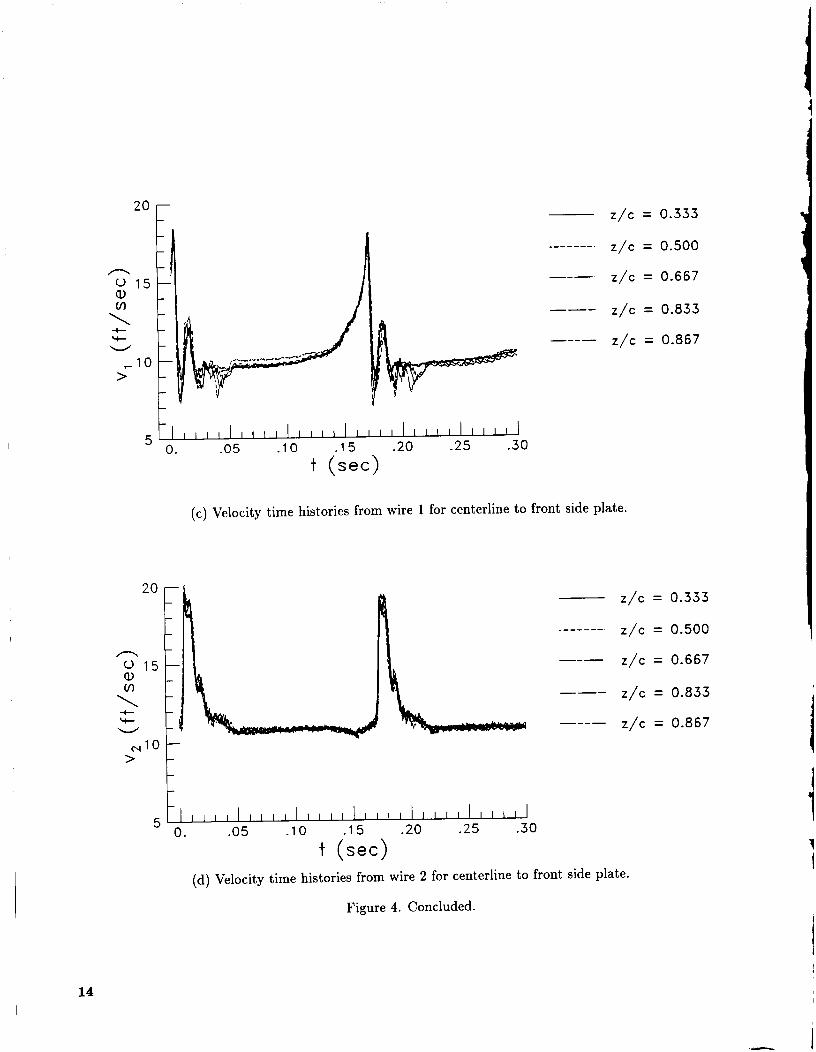
Ideally, a two-dimensional flow field is invariant in one dimension, in this case the z-direction. Of course, a real flow may be influenced by such factors as boundary layer effects and vortex filament twisting. An attempt to assess the invariance of the velocity field in the z-direction was made by sampling the velocity at a fixed z,y point in various z-planes. The data, in the form of velocity time histories, are presented in figure 4. The data presented were obtained at z/c = 1.0, y/c = 0.333 with the tailored wake as the incident flow.

In figure 4(a), the velocity normal to wire 1 is presented for several stations between the centerline of the test section and the back side plate. It is immediately evident that the velocity time histories at all stations are very similar. The two large velocity variations occurring at the start of the data record and around 0.17 sec are the result of a vortex passage. Notice that, with the exception of the data taken at z /c = -0.917 (0.5 in. away from the rear side plate), the amplitude and timing of the velocity variation are invariant with z-station. This indicates that the flow is two-dimensional from the centerline to within an inch of the side plate. Delay of the velocity variation because of the vortex passage at the z / c = -0.917 station indicates that the boundary layer on the side plate is tending to bend the end of the vortex structure as it drags against the solid surface in the boundary layer. Figure 4(b), which depicts the velocity normal to the other wire in the cross-wire probe, shows a similar trend, although the delay caused by the side plate boundary layer is not as evident.

Figure 4(c) contains the velocity survey from the centerline to the front side plate. Of interest is the fact that a delayed velocity variation is not as evident in the data nearest the side plate, although the smearing of the velocity time history in a sec- ondary minima occurring around 0.21 sec grows pro- gressively worse as the side plate is approached. One possible explanation for the lack of the delay feature could be that the survey was not performed as close to the side plate as for the previous case because of interference between the side plate and the probe mount. Note that the data for the z / c = 0.500 station were obtained on a different day from the re- mainder of the data in the figure, and the 0.5 ft/sec difference in the mean velocity data is probably representative of typical day-to-day repeatability of the data. Figure 4(d), containing the velocity normal to the other wire in the probe, shows little variation with z-station.

From the data presented, one may conclude that the wake produced by the pitching airfoil is indeed two-dimensional for a large portion of the test section span.

Survey of Sinusoidal Wake Initially, in the two-dimensional blade-vortex

study, the wake produced by oscillating the airfoil sinusoidally at 30 cycles/sec was used as the test flow. In this section, the wake produced by those conditions will be examined.

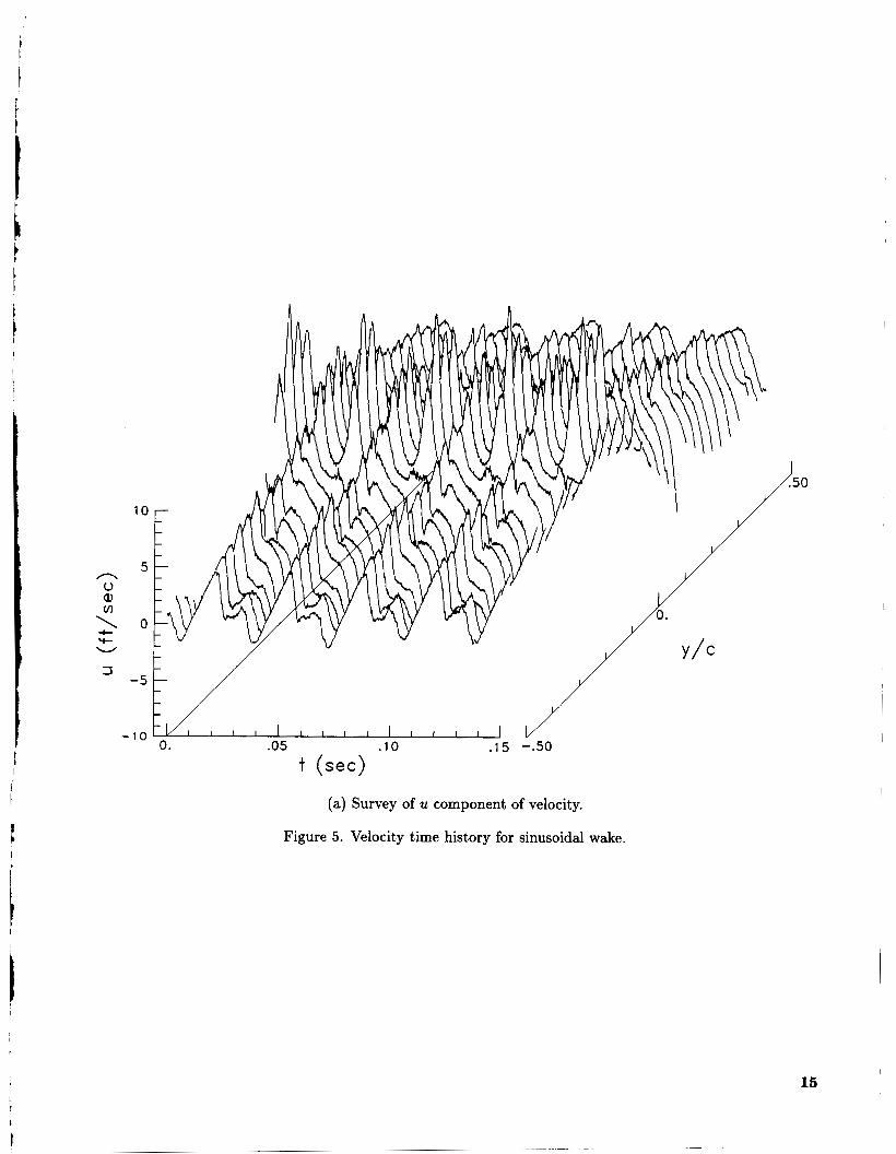
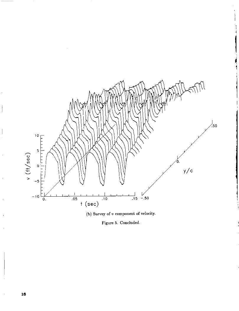
Velocity fierd. The velocity field produced by the sinusoidal oscillation case is presented in figure 5. In figure 5(a), the u velocity component is shown to be periodic, with a period of approximately 0.033 sec, which corresponds to an oscillation frequency of 30 Hz and (at a free-stream velocity of 15 ft/sec) a spatial separation of IC. Another item of note is that the amplitude of the u velocity component reaches a maximum very near the center of the flow field. Figure 5(b) displays similar trends for the v velocity field. Another interesting feature in the ZI component data is that the shape of the velocity time history curves changes at approximately the center of the test section to a near mirror image; this indicates that the flow features in one-half of the flow are nearly opposite and equal to what is hap- pening in the other half of the flow. Actually, this is a consequence of the fact that the sinusoidal oscillation produces a train of vortices of alternating sign and nearly equal magnitude.

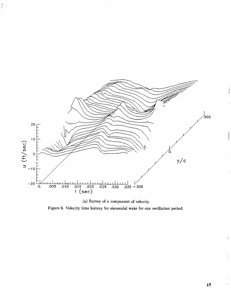
Examination of the velocity field for a single cycle is useful to gain a more thorough understanding of the flow field. In figure 6, velocity data for each component are displayed for a single cycle. In

5

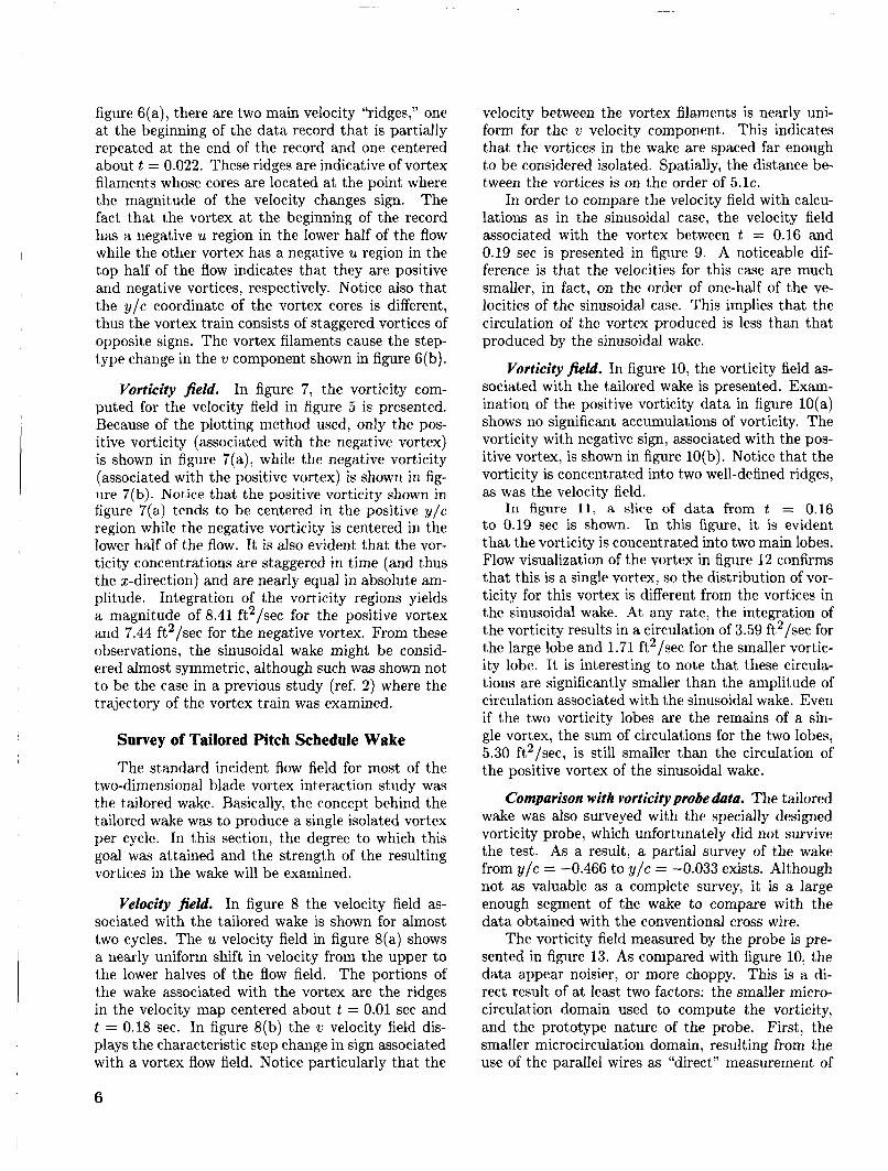
figure 6(a), there are two main velocity “ridges,” one at the beginning of the data record that is partially repeated at the end of the record and one centered about t = 0.022. These ridges are indicative of vortex filaments whose cores are located at the point where the magnitude of the velocity changes sign. The fact that the vortex at the beginning of the record has a negative u region in the lower half of the flow while the other vortex has a negative u region in the top half of the flow indicates that they are positive and negative vortices, respectively. Notice also that the y/c coordinate of the vortex cores is different, thus the vortex train consists of staggered vortices of opposite signs. The vortex filaments cause the step- type change in the ?J component shown in figure 6(b).

Vorticity field. In figure 7, the vorticity computed for the velocity field in figure 5 is presented. Because of the plotting method used, only the positive vorticity (associated with the negative vortex) is shown in figure 7(a), while the negative vorticity (associated with the positive vortex) is shown in figure 7(b). Notice that the positive vorticity shown in figure 7(a) tends to be centered in the positive y/c region while the negative vorticity is centered in the lower half of the flow. It is also evident that the vorticity concentrations are staggered in time (and thus the 2-direction) and are nearly equal in absolute amplitude. Integration of the vorticity regions yields a magnitude of 8.41 ft2/sec for the positive vortex and 7.44 ft2/sec for the negative vortex. From these observations, the sinusoidal wake might be considered almost symmetric, although such was shown not to be the case in a previous study (ref. 2) where the trajectory of the vortex train was examined.

Survey of Tailored Pitch Schedule Wake The standard incident flow field for most of the

two-dimensional blade vortex interaction study was the tailored wake. Basically, the concept behind the tailored wake was to produce a single isolated vortex per cycle. In this section, the degree to which this goal was attained and the strength of the resulting vortices in the wake will be examined.

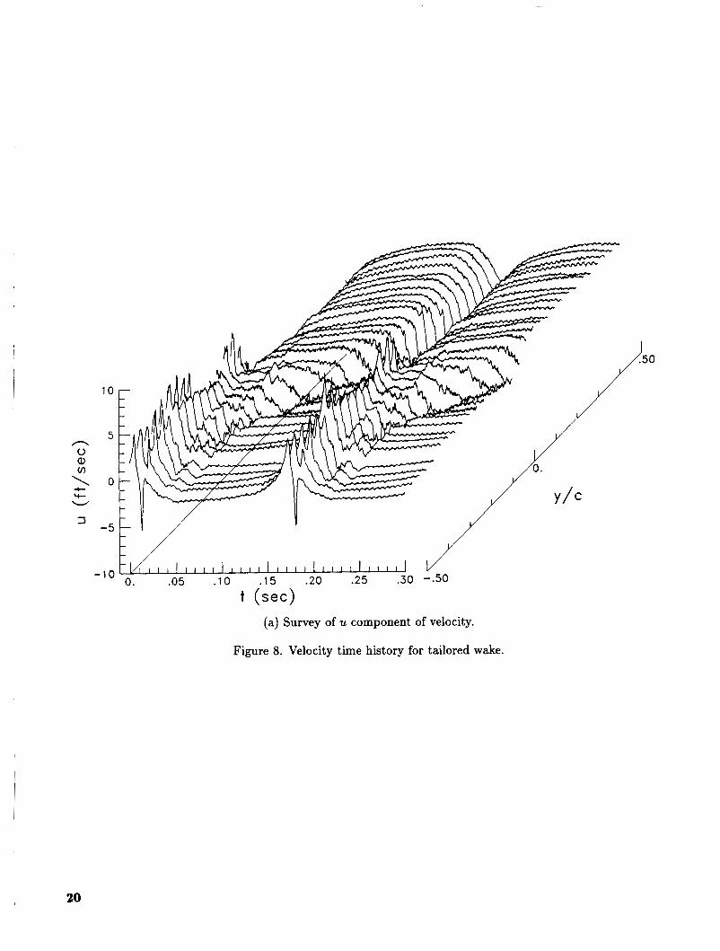
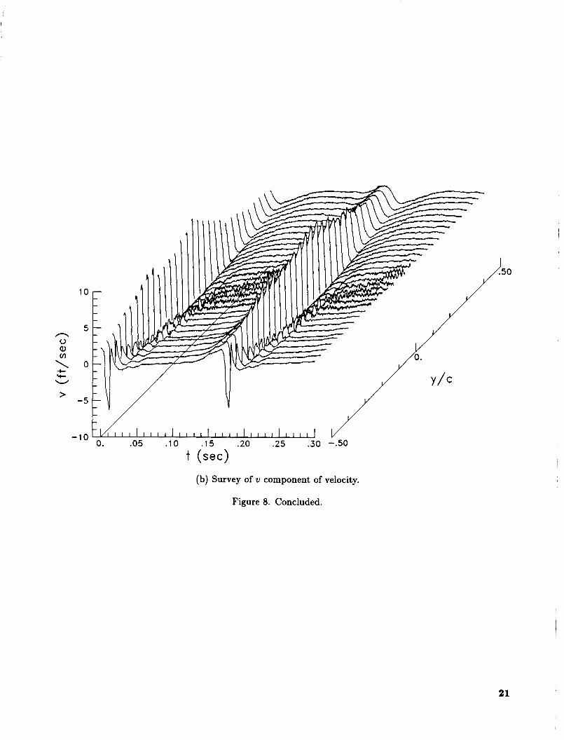
Velocity fieZd. In figure 8 the velocity field associated with the tailored wake is shown for almost two cycles. The u velocity field in figure 8(a) shows a nearly uniform shift in velocity from the upper to the lower halves of the flow field. The portions of the wake associated with the vortex are the ridges in the velocity map centered about t = 0.01 sec and t = 0.18 sec. In figure 8(b) the ?J velocity field displays the characteristic step change in sign associated with a vortex flow field. Notice particularly that the

velocity between the vortex filaments is nearly uniform for the u velocity component. This indicates that the vortices in the wake are spaced far enough to be considered isolated. Spatially, the distance between the vortices is on the order of 5 . 1 ~ .

In order to compare the velocity field with calcu- lations as in the sinusoidal case, the velocity field associated with the vortex between t = 0.16 and 0.19 sec is presented in figure 9. A noticeable difference is that the velocities for this case are much smaller, in fact, on the order of one-half of the velocities of the sinusoidal case. This implies that the circulation of the vortex produced is less than that produced by the sinusoidal wake.

Vorticity fieZd. In figure 10, the vorticity field associated with the tailored wake is presented. Exam- ination of the positive vorticity data in figure lO(a) shows no significant accumulations of vorticity. The vorticity with negative sign, associated with the positive vortex, is shown in figure 10(b). Notice that the vorticity is concentrated into two well-defined ridges, as was the velocity field.

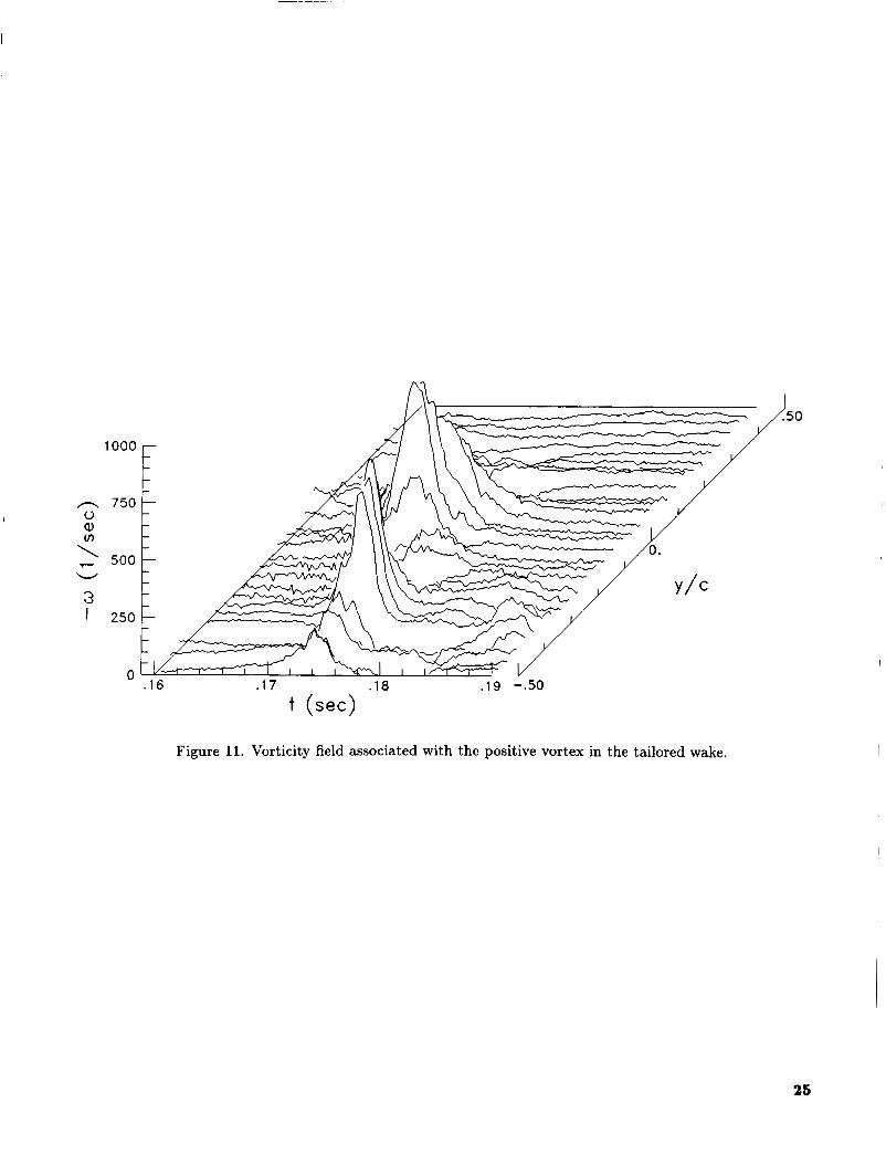
In figure 11, a slice of data from t = 0.16 to 0.19 sec is shown. In this figure, it is evident that the vorticity is concentrated into two main lobes. Flow visualization of the vortex in figure 12 confirms that this is a single vortex, so the distribution of vorticity for this vortex is different from the vortices in the sinusoidal wake. At any rate, the integration of the vorticity results in a circulation of 3.59 ft2/sec for the large lobe and 1.71 ft2/sec for the smaller vorticity lobe. It is interesting to note that these circulations are significantly smaller than the amplitude of circulation associated with the sinusoidal wake. Even if the two vorticity lobes are the remains of a single vortex, the sum of circulations for the two lobes, 5.30 ft2/sec, is still smaller than the circulation of the positive vortex of the sinusoidal wake.

Comparison with vorticity probe data. The tailored wake was also surveyed with the specially designed vorticity probe, which unfortunately did not survive the test. As a result, a partial survey of the wake from y/c = -0.466 to y/c = -0.033 exists. Although not as valuable as a complete survey, it is a large enough segment of the wake to compare with the data obtained with the conventional cross wire.

The vorticity field measured by the probe is presented in figure 13. As compared with figure 10, the data appear noisier, or more choppy. This is a direct result of at least two factors: the smaller microcirculation domain used to compute the vorticity, and the prototype nature of the probe. First, the smaller microcirculation domain, resulting from the use of the parallel wires as “direct” measurement of

6

the du/dy term, is less numerically stable. In equation (lo), the magnitudes of the denominator terms decrease by an order of magnitude, therefore, a given error in the numerator terms is magnified by that order of magnitude. A second reason for the noisier data is the prototype nature of the probe, being itself a research project instead of a commercial product. A commercially designed and manufactured vorticity probe probably would exhibit cleaner output data as well as being a bit more rugged.

Two interesting features of the data in figure 13 are that the magnitudes of the negative vorticity peaks are much greater than those in figure 10 and that the negative vorticity peaks in figure 13 are ac- companied by adjoining positive vorticity peaks that are not at all evident in figure 10. A possible explanation of this may be that the increase in spatial resolution inherent in the vorticity probe is de- tecting real flow features that were smeared over by the conventional probe. A method of testing this hypothesis is to compute the circulation over a selected area in both data sets and compare the results. The region selected is bounded by t = 0.15 sec, t = 0.21 sec, y/c = -0.466, and y/c = -0.033. The resulting values of circulation are 0.272 ft2/sec for the vorticity probe as compared with 0.340 ft2/sec for the cross wire. Since these values are similar, the additional vorticity features are probably due to the spatial resolution of the vorticity probe. Further development of the vorticity probe is therefore war- ranted for measurements where the additional resolution of the probe is required.

Summary of Results The velocity field produced by an airfoil oscillat-

ing about its quarter-chord has been surveyed by using hot-wire anemometry. The velocity field was used to calculate the vorticity in the wake, which was used to calculate the circulation of the coherent vortex filaments embedded in the wake. These data were examined to characterize the vortex wake for two conditions relevant to a two-dimensional blade- vortex investigation.

Examination of velocity time histories taken at several spanwise locations verifies that the velocity field is two-dimensional for a large portion of the span of the test section.

Data from the sinusoidal wake reveal that the wake is composed of staggered vortices of opposite sign and nearly equal amplitude. The spacing of adjacent vortices of like sign is on the order of IC (the chord length of the vortex generator). The amplitude

of the circulation of the negative vortex is 7.44 ft2/sec and that of the positive vortex is 8.41 ft2/sec.

The velocity field produced by the tailored wake shows that the vortex filaments are not as strong as for the sinusoidal wake and are separated by about 5. IC. Although prominent positive vortices are present in the tailored wake, no strong negative vortex is evident. The positive vortex feature appears in the vorticity data as two distinct vorticity accumulations, although flow visualization data show only a single vortex feature. The circulation of the vortex is 5.30 ft2/sec.

The vorticity data measured with a prototype vorticity probe exhibit more numerical noise, which has been ascribed to the smaller measurement domain and the prototype nature of the probe. The vorticity probe data reveal details in the vorticity field not evident in the cross-wire data because of the greater spatial resolution of the probe. Magni- tude differences in the vorticity data are the result of the smaller measurement volume used by the probe. Integration of vorticity over an area in both data sets produced similar values of circulation.

NASA Langley Research Center Hampton, Virginia 23665-5225 November 5, 1987

References 1.

2.

3.

4.

5.

6.

7.

8.

9.

Booth, Earl R., Jr.; and Yu, James C.: New Technique for Experimental Generation of Two-Dimensional Blade- Vortex Interaction at Low Reynolds Numbers. NASA

Booth, E. R., Jr.; and Yu, J. C.: Two-Dimensional Blade-Vortex Flow Visualization Investigation. A I A A J. , vol. 24, no. 9, Sept. 1986, pp. 1468-1473. Booth, Earl R., Jr.: Surface Pressure Measurement Dur- ing Low Speed Two-Dimensional Blade-Vortex Inter- action. AIAA-861856, July 1986. Hubbard, Harvey H.; and Manning, James C.: Aero- acoustic Research Facilities at N A S A Langley Research Center-Description and Operational Characteristics.

D I S A Probe Catalog. Publ. No. 2201 E, Dantec Elec- tronics Inc., Mar. 1982. Foss, John F.; Klewicki, Casey L.; and Disimile, Peter J.: Transverse Vorticity Measurements Using a n Array of Four Hot- Wire Probes. NASA CR-178098, 1986. Hardin, Jay C.: Introduction to T ime Series Analysis.

Liepmann, H. W.; and Roshko, A.: Elements of Gas- dynamics. John Wiley & Sons, Inc., c.1957. Kuethe, Arnold M.; and Chow, Chuen-Yen: Foundations of Aerodynamics: Bases of Aerodynamic Design, Third ed. John Wiley & Sons, c.1976.

TP-2551, 1986.

NASA TM-84585, 1983.

NASA RP-1145, 1986.

7

Positive U, fY vortex

I n

Oscillating airfoil

Negative vortex

y/C = 0.5

T Survey line x/c= 1.0 t

1 y/C = - 0.5

Figure 1. Sketch of coordinate system used in the experiment.

I Ht

11

2o F Z/C = -0.333

n 0 0 < + cc W

F

>

15

10

Z/C = -0.500

Z/C = -0.667

Z/C = -0.833

Z/C = -0.917

0. .05 .10 .15 .20 .25 .30 5 I I i I I I I I I I ' I 1 l l ' I I i I ' I I I I ( I I I I I

t (sec) (a) Velocity time histories from wire 1 for centerline t o rear side plate.

20 r

(b) Velocity time histories from wire 2 for centerline to rear side plate.

Z/C = -0.333

Z/C = -0.500

Z/C = -0.667

Z/C = -0.833

Z/C = -0.917

Figure 4. Velocity time histories across the test section.

z/c = 0.333

t ( s e c )

(c) Velocity time histories from wire 1 for centerline to front side plate.

20 z/c = 0.333

z/c = 0.500

z/c = 0.667

z/c = 0.833

z/c = 0.867

i 1 .25 .30 0. .05 .10 .15 .20 5

t (sec) (d) Velocity time histories from wire 2 for centerline to front side plate.

Figure 4. Concluded.

7 1

14

I

t

I I I I I l l 1 I l l 1 -10 0. .05 .10 .15 -.50

t (sec)

(a) Survey of u component of velocity.

Figure 5. Velocity time history for sinusoidal wake.

1 5 0

15

10

5

i 1

n 0 a, v,

\ o c

> -5

-10

t (sec)

(b) Survey of v component of velocity.


16

20

10 n V a, v)

\ o + 't v

3 -10

t ( s e c )


Figure 6. Velocity time history for sinusoidal wake for one oscillation period.

17

n *O 10 E 0 a, v,

\ o + + W

> -10

- 20

t (sec)

(b) Survey of IJ component of velocity.


18

!50

t (sec)

(a) Positive vorticity field.

!50

2000

1500 A 0 0 v)

\ 1000 7

W

3 I 500

0

t (sec)

(b) Negative vorticity field.

Figure 7. Vorticity field survey for sinusoidal wake.

19

!50

n 0 a, v)

\ t + v

S

10

5

0

-5


Figure 8. Velocity time history for tailored wake.

20

10

5 n 0 Q,

< o + Y- W

> -5

-10 0. .05 .10 .15 .20 -25 .30 -.SO

t (sec)



21

10

5

\ o c

I l l 1 I l l 1 I l l 1 -10 .17 . I a .19 -050 .16

t (sec)


Figure 9. Velocity time history for tailored wake.

22

10

5 n

> -5

-10

t (sec)



23

1

1000

0 a, ul \ 500 W

t (sec)


A 0 a, v)

\

3 I

- W

50

t (sec)


Figure 10. Vorticity field for tailored wake.

24

50

1000

n 750 0 Q, v, > 500

W

3 I 250

.16 .17 .18 0

t (sec)

Figure 11. Vorticity field associated with the positive vortex in the tailored wake.

25

n 0 a, v)

\ 7

W

I

3

1500

1000

500

0

A 1500 u a, v) > 1000

W

)O.

Y/C

t (sec)


0


Figure 13. Vorticity field measured by vorticity probe.

27

N/\sJ\ Nalional AeronauliCS and Report Documentation Page

1. Report No. NASA TP-2780

2. Government Accession No.

7. Author(s) Earl R. Booth, Jr

19. Security Classif.(of this report) Unclassified

3. Performing Organization Name and Address NASA Langley Research Center Hampton, VA 23665-5225

20. Security Classif.(of this page) 21. No. of Pages 22. Price Unclassified 28 A03

12. Sponsoring Agency Name and Address National Aeronautics and Space Administration Washington, DC 20546-0001

15. Supplementary Notes

3. Recipient’s Catalog No.

5. Report Date

December 1987 6. Performing Organization Code

8. Performing Organization Report No.

L-16339 10. Work Unit No.

505-61-51-06 11. Contract or Grant No.

13. Type of Report and Period Covered

Technical Paper 14. Sponsoring Agency Code

16. Abstract The velocity field created by the wake of an airfoil undergoing a prescribed pitching motion was sampled by using hot-wire anemometry. Data analysis methods concerning resolution of velocity components from cross-wire data, computation of vorticity from velocity time history data, and calculation of vortex circulation from vorticity field data are discussed. These data analysis methods are applied to a flow field relevant to a two-dimensional blade-vortex interaction study. Velocity time history data were differentiated to yield vorticity field data, which were used to characterize the wake of the pitching airfoil. Measurements of vortex strength in sinusoidal and nonsinusoidal wakes show vortices in the sinusoidal wake have stronger circulation and more concentrated vorticity distributions than the tailored nonsinusoidal wake. Also, the tailored nonsinusoidal wake exhibited separation of positive vortices of the order of five times the chord length of the vortex generator, while vortices of the opposite sign were effectively suppressed. In addition, some data are presented which were obtained with a specially designed vorticity probe, which yielded greater spatial resolution than the conventional cross-wire method.

17. Key Words (Suggested by Authors(s)) Vorticity Oscillating airfoil wake Hot-wire anemometry Vortex circulation

18. Distribution Statement Unclassified-Unlimited

Subject Category 71

987 measurement of velocity and vorticity fields in j the ... · pdf filemeasurement of...

Documents