7 energy resources and potentials - iiasa · maurice b. dusseault (university of waterloocanada) ,...
TRANSCRIPT

425
Energy Resources and Potentials
Convening Lead Author (CLA) Hans-Holger Rogner (International Atomic Energy Agency, Austria)
Lead Authors (LA) Roberto F. Aguilera (Curtin University, Australia) Cristina L. Archer (California State University and Stanford University, USA) Ruggero Bertani (Enel Green Power S.p.A., Italy) S.C. Bhattacharya (International Energy Initiative, India) Maurice B. Dusseault (University of Waterloo, Canada) Luc Gagnon (HydroQu é bec, Canada) Helmut Haberl (Klagenfurt University, Austria) Monique Hoogwijk (Ecofys, the Netherlands) Arthur Johnson (Hydrate Energy International, USA) Mathis L. Rogner (International Institute for Applied Systems Analysis, Austria) Horst Wagner (Montan University Leoben, Austria) Vladimir Yakushev (Gazprom, Russia)
Contributing Authors (CA) Doug J. Arent (National Renewable Energy Laboratory, USA) Ian Bryden (University of Edinburgh, UK) Fridolin Krausmann (Klagenfurt University, Austria) Peter Odell (Erasmus University Rotterdam, the Netherlands) Christoph Schillings (German Aerospace Center) Ali Shafi ei (University of Waterloo, Canada)
Review Editor Ji Zou (Renmin University of China)
7

Energy Resources and Potentials Chapter 7
Contents
426
Contents
Executive Summary . . . . . . . . . . . . . . . . . . . . . . . . . . . . . . . . . . . . . . . . . . . . . . . . . . . . . . . . . . . . . . . . . . . . . . . . . . . . . . . . . . . . . . . . . . . . . . . . . . . . . . . . . . . . . . . . . . . . . . . . . . . . . . . . . . . . . . . . . . . . . . . . . . . . . . . . . . . . 430
Hydrocarbons and Nuclear . . . . . . . . . . . . . . . . . . . . . . . . . . . . . . . . . . . . . . . . . . . . . . . . . . . . . . . . . . . . . . . . . . . . . . . . . . . . . . . . . . . . . . . . . . . . . . . . . . . . . . . . . . . . . . . . . . . . . . . . . . . . . . . . . . . . . . . . . . . . . . . . . . . . . . . . . . 430
Renewables . . . . . . . . . . . . . . . . . . . . . . . . . . . . . . . . . . . . . . . . . . . . . . . . . . . . . . . . . . . . . . . . . . . . . . . . . . . . . . . . . . . . . . . . . . . . . . . . . . . . . . . . . . . . . . . . . . . . . . . . . . . . . . . . . . . . . . . . . . . . . . . . . . . . . . . . . . . . . . . . . . . . . . . . . . . . . . . . 431
7.1 Introduction . . . . . . . . . . . . . . . . . . . . . . . . . . . . . . . . . . . . . . . . . . . . . . . . . . . . . . . . . . . . . . . . . . . . . . . . . . . . . . . . . . . . . . . . . . . . . . . . . . . . . . . . . . . . . . . . . . . . . . . . . . . . . . . . . . . . . . . . . . . . . . . . . . . . . . . . 433
7.1.1 Defi nitions and Classifi cations . . . . . . . . . . . . . . . . . . . . . . . . . . . . . . . . . . . . . . . . . . . . . . . . . . . . . . . . . . . . . . . . . . . . . . . . . . . . . . . . . . . . . . . . . . . . . . . . . . . . . . . . . . . . . . . . . . . . . . . . . . . . . . . . . . 433
7.1.2 The ‘Peak Debate’ . . . . . . . . . . . . . . . . . . . . . . . . . . . . . . . . . . . . . . . . . . . . . . . . . . . . . . . . . . . . . . . . . . . . . . . . . . . . . . . . . . . . . . . . . . . . . . . . . . . . . . . . . . . . . . . . . . . . . . . . . . . . . . . . . . . . . . . . . . . . . . . . . . . . . 435
7.1.3 Units of Measurement . . . . . . . . . . . . . . . . . . . . . . . . . . . . . . . . . . . . . . . . . . . . . . . . . . . . . . . . . . . . . . . . . . . . . . . . . . . . . . . . . . . . . . . . . . . . . . . . . . . . . . . . . . . . . . . . . . . . . . . . . . . . . . . . . . . . . . . . . . . . . . 437
7.2 Oil . . . . . . . . . . . . . . . . . . . . . . . . . . . . . . . . . . . . . . . . . . . . . . . . . . . . . . . . . . . . . . . . . . . . . . . . . . . . . . . . . . . . . . . . . . . . . . . . . . . . . . . . . . . . . . . . . . . . . . . . . . . . . . . . . . . . . . . . . . . . . . . . . . . . . . . . . . . . . . . . . . . . . . . . . . . 438
7.2.1 Overview . . . . . . . . . . . . . . . . . . . . . . . . . . . . . . . . . . . . . . . . . . . . . . . . . . . . . . . . . . . . . . . . . . . . . . . . . . . . . . . . . . . . . . . . . . . . . . . . . . . . . . . . . . . . . . . . . . . . . . . . . . . . . . . . . . . . . . . . . . . . . . . . . . . . . . . . . . . . . . . . . . 438
7.2.2 Estimates of Conventional Oil . . . . . . . . . . . . . . . . . . . . . . . . . . . . . . . . . . . . . . . . . . . . . . . . . . . . . . . . . . . . . . . . . . . . . . . . . . . . . . . . . . . . . . . . . . . . . . . . . . . . . . . . . . . . . . . . . . . . . . . . . . . . . . . . . . . 439
7.2.3 Types of Unconventional Oil . . . . . . . . . . . . . . . . . . . . . . . . . . . . . . . . . . . . . . . . . . . . . . . . . . . . . . . . . . . . . . . . . . . . . . . . . . . . . . . . . . . . . . . . . . . . . . . . . . . . . . . . . . . . . . . . . . . . . . . . . . . . . . . . . . . . . 441
7.2.4 Estimates of Unconventional Oil . . . . . . . . . . . . . . . . . . . . . . . . . . . . . . . . . . . . . . . . . . . . . . . . . . . . . . . . . . . . . . . . . . . . . . . . . . . . . . . . . . . . . . . . . . . . . . . . . . . . . . . . . . . . . . . . . . . . . . . . . . . . . . . 443
7.2.5 Oil Supply Cost Curves . . . . . . . . . . . . . . . . . . . . . . . . . . . . . . . . . . . . . . . . . . . . . . . . . . . . . . . . . . . . . . . . . . . . . . . . . . . . . . . . . . . . . . . . . . . . . . . . . . . . . . . . . . . . . . . . . . . . . . . . . . . . . . . . . . . . . . . . . . . . . . 444
7.2.6 Environmental and Social Implications . . . . . . . . . . . . . . . . . . . . . . . . . . . . . . . . . . . . . . . . . . . . . . . . . . . . . . . . . . . . . . . . . . . . . . . . . . . . . . . . . . . . . . . . . . . . . . . . . . . . . . . . . . . . . . . . . . . . . . 445
7.2.7 Summary . . . . . . . . . . . . . . . . . . . . . . . . . . . . . . . . . . . . . . . . . . . . . . . . . . . . . . . . . . . . . . . . . . . . . . . . . . . . . . . . . . . . . . . . . . . . . . . . . . . . . . . . . . . . . . . . . . . . . . . . . . . . . . . . . . . . . . . . . . . . . . . . . . . . . . . . . . . . . . . . . . 450
7.3 Natural Gas . . . . . . . . . . . . . . . . . . . . . . . . . . . . . . . . . . . . . . . . . . . . . . . . . . . . . . . . . . . . . . . . . . . . . . . . . . . . . . . . . . . . . . . . . . . . . . . . . . . . . . . . . . . . . . . . . . . . . . . . . . . . . . . . . . . . . . . . . . . . . . . . . . . . . . . . . 450
7.3.1 Overview . . . . . . . . . . . . . . . . . . . . . . . . . . . . . . . . . . . . . . . . . . . . . . . . . . . . . . . . . . . . . . . . . . . . . . . . . . . . . . . . . . . . . . . . . . . . . . . . . . . . . . . . . . . . . . . . . . . . . . . . . . . . . . . . . . . . . . . . . . . . . . . . . . . . . . . . . . . . . . . . . . 450
7.3.2 Classifying Conventional Gas and Unconventional Gas . . . . . . . . . . . . . . . . . . . . . . . . . . . . . . . . . . . . . . . . . . . . . . . . . . . . . . . . . . . . . . . . . . . . . . . . . . . . . . . . . . . . . . . . . . . . . . 450
7.3.3 Conventional Natural Gas Reserves and Resources . . . . . . . . . . . . . . . . . . . . . . . . . . . . . . . . . . . . . . . . . . . . . . . . . . . . . . . . . . . . . . . . . . . . . . . . . . . . . . . . . . . . . . . . . . . . . . . . . . . 451
7.3.4 Unconventional Gas . . . . . . . . . . . . . . . . . . . . . . . . . . . . . . . . . . . . . . . . . . . . . . . . . . . . . . . . . . . . . . . . . . . . . . . . . . . . . . . . . . . . . . . . . . . . . . . . . . . . . . . . . . . . . . . . . . . . . . . . . . . . . . . . . . . . . . . . . . . . . . . . . . 453
7.3.5 Resource Estimates for Unconventional Gas Resources (Excluding Gas Hydrate) . . . . . . . . . . . . . . . . . . . . . . . . . . . . . . . . . . . . . . . . . . . . . . . . . . . . . . . . 455
7.3.6 Gas Hydrate . . . . . . . . . . . . . . . . . . . . . . . . . . . . . . . . . . . . . . . . . . . . . . . . . . . . . . . . . . . . . . . . . . . . . . . . . . . . . . . . . . . . . . . . . . . . . . . . . . . . . . . . . . . . . . . . . . . . . . . . . . . . . . . . . . . . . . . . . . . . . . . . . . . . . . . . . . . . . 455
Chapter 7 Energy Resources and Potentials
427
7.3.7 Abiogenic Gas Theory . . . . . . . . . . . . . . . . . . . . . . . . . . . . . . . . . . . . . . . . . . . . . . . . . . . . . . . . . . . . . . . . . . . . . . . . . . . . . . . . . . . . . . . . . . . . . . . . . . . . . . . . . . . . . . . . . . . . . . . . . . . . . . . . . . . . . . . . . . . . . . . 458
7.3.8 Natural Gas Supply Cost Curves . . . . . . . . . . . . . . . . . . . . . . . . . . . . . . . . . . . . . . . . . . . . . . . . . . . . . . . . . . . . . . . . . . . . . . . . . . . . . . . . . . . . . . . . . . . . . . . . . . . . . . . . . . . . . . . . . . . . . . . . . . . . . . . . 459
7.3.9 Environmental and Social Implications . . . . . . . . . . . . . . . . . . . . . . . . . . . . . . . . . . . . . . . . . . . . . . . . . . . . . . . . . . . . . . . . . . . . . . . . . . . . . . . . . . . . . . . . . . . . . . . . . . . . . . . . . . . . . . . . . . . . . . 460
7.3.10 Summary . . . . . . . . . . . . . . . . . . . . . . . . . . . . . . . . . . . . . . . . . . . . . . . . . . . . . . . . . . . . . . . . . . . . . . . . . . . . . . . . . . . . . . . . . . . . . . . . . . . . . . . . . . . . . . . . . . . . . . . . . . . . . . . . . . . . . . . . . . . . . . . . . . . . . . . . . . . . . . . . . . 460
7.4 Coal . . . . . . . . . . . . . . . . . . . . . . . . . . . . . . . . . . . . . . . . . . . . . . . . . . . . . . . . . . . . . . . . . . . . . . . . . . . . . . . . . . . . . . . . . . . . . . . . . . . . . . . . . . . . . . . . . . . . . . . . . . . . . . . . . . . . . . . . . . . . . . . . . . . . . . . . . . . . . . . . . . . . . . . . 461
7.4.1 Overview . . . . . . . . . . . . . . . . . . . . . . . . . . . . . . . . . . . . . . . . . . . . . . . . . . . . . . . . . . . . . . . . . . . . . . . . . . . . . . . . . . . . . . . . . . . . . . . . . . . . . . . . . . . . . . . . . . . . . . . . . . . . . . . . . . . . . . . . . . . . . . . . . . . . . . . . . . . . . . . . . . 461
7.4.2 Coal Production . . . . . . . . . . . . . . . . . . . . . . . . . . . . . . . . . . . . . . . . . . . . . . . . . . . . . . . . . . . . . . . . . . . . . . . . . . . . . . . . . . . . . . . . . . . . . . . . . . . . . . . . . . . . . . . . . . . . . . . . . . . . . . . . . . . . . . . . . . . . . . . . . . . . . . . . 461
7.4.3 Reserves . . . . . . . . . . . . . . . . . . . . . . . . . . . . . . . . . . . . . . . . . . . . . . . . . . . . . . . . . . . . . . . . . . . . . . . . . . . . . . . . . . . . . . . . . . . . . . . . . . . . . . . . . . . . . . . . . . . . . . . . . . . . . . . . . . . . . . . . . . . . . . . . . . . . . . . . . . . . . . . . . . . 461
7.4.4 Resources . . . . . . . . . . . . . . . . . . . . . . . . . . . . . . . . . . . . . . . . . . . . . . . . . . . . . . . . . . . . . . . . . . . . . . . . . . . . . . . . . . . . . . . . . . . . . . . . . . . . . . . . . . . . . . . . . . . . . . . . . . . . . . . . . . . . . . . . . . . . . . . . . . . . . . . . . . . . . . . . . 463
7.4.5 Coal Mining Technology . . . . . . . . . . . . . . . . . . . . . . . . . . . . . . . . . . . . . . . . . . . . . . . . . . . . . . . . . . . . . . . . . . . . . . . . . . . . . . . . . . . . . . . . . . . . . . . . . . . . . . . . . . . . . . . . . . . . . . . . . . . . . . . . . . . . . . . . . . . . 464
7.4.6 Coal Mining Costs . . . . . . . . . . . . . . . . . . . . . . . . . . . . . . . . . . . . . . . . . . . . . . . . . . . . . . . . . . . . . . . . . . . . . . . . . . . . . . . . . . . . . . . . . . . . . . . . . . . . . . . . . . . . . . . . . . . . . . . . . . . . . . . . . . . . . . . . . . . . . . . . . . . . . 465
7.4.7 Coal Supply Cost Curves . . . . . . . . . . . . . . . . . . . . . . . . . . . . . . . . . . . . . . . . . . . . . . . . . . . . . . . . . . . . . . . . . . . . . . . . . . . . . . . . . . . . . . . . . . . . . . . . . . . . . . . . . . . . . . . . . . . . . . . . . . . . . . . . . . . . . . . . . . . 466
7.4.8 Environmental and Social Implications . . . . . . . . . . . . . . . . . . . . . . . . . . . . . . . . . . . . . . . . . . . . . . . . . . . . . . . . . . . . . . . . . . . . . . . . . . . . . . . . . . . . . . . . . . . . . . . . . . . . . . . . . . . . . . . . . . . . . . 466
7.4.9 Summary . . . . . . . . . . . . . . . . . . . . . . . . . . . . . . . . . . . . . . . . . . . . . . . . . . . . . . . . . . . . . . . . . . . . . . . . . . . . . . . . . . . . . . . . . . . . . . . . . . . . . . . . . . . . . . . . . . . . . . . . . . . . . . . . . . . . . . . . . . . . . . . . . . . . . . . . . . . . . . . . . . 467
7.5 Nuclear Resource Materials . . . . . . . . . . . . . . . . . . . . . . . . . . . . . . . . . . . . . . . . . . . . . . . . . . . . . . . . . . . . . . . . . . . . . . . . . . . . . . . . . . . . . . . . . . . . . . . . . . . . . . . . . . . . . . . . . . . . . . . . . . . 468
7.5.1 Overview . . . . . . . . . . . . . . . . . . . . . . . . . . . . . . . . . . . . . . . . . . . . . . . . . . . . . . . . . . . . . . . . . . . . . . . . . . . . . . . . . . . . . . . . . . . . . . . . . . . . . . . . . . . . . . . . . . . . . . . . . . . . . . . . . . . . . . . . . . . . . . . . . . . . . . . . . . . . . . . . . . 468
7.5.2 Uranium . . . . . . . . . . . . . . . . . . . . . . . . . . . . . . . . . . . . . . . . . . . . . . . . . . . . . . . . . . . . . . . . . . . . . . . . . . . . . . . . . . . . . . . . . . . . . . . . . . . . . . . . . . . . . . . . . . . . . . . . . . . . . . . . . . . . . . . . . . . . . . . . . . . . . . . . . . . . . . . . . . . 468
7.5.3 Thorium . . . . . . . . . . . . . . . . . . . . . . . . . . . . . . . . . . . . . . . . . . . . . . . . . . . . . . . . . . . . . . . . . . . . . . . . . . . . . . . . . . . . . . . . . . . . . . . . . . . . . . . . . . . . . . . . . . . . . . . . . . . . . . . . . . . . . . . . . . . . . . . . . . . . . . . . . . . . . . . . . . . 472
7.5.4 Fusion Materials . . . . . . . . . . . . . . . . . . . . . . . . . . . . . . . . . . . . . . . . . . . . . . . . . . . . . . . . . . . . . . . . . . . . . . . . . . . . . . . . . . . . . . . . . . . . . . . . . . . . . . . . . . . . . . . . . . . . . . . . . . . . . . . . . . . . . . . . . . . . . . . . . . . . . . . 473
7.5.5 Environmental and Social Implications . . . . . . . . . . . . . . . . . . . . . . . . . . . . . . . . . . . . . . . . . . . . . . . . . . . . . . . . . . . . . . . . . . . . . . . . . . . . . . . . . . . . . . . . . . . . . . . . . . . . . . . . . . . . . . . . . . . . . . 474
7.5.6 Summary . . . . . . . . . . . . . . . . . . . . . . . . . . . . . . . . . . . . . . . . . . . . . . . . . . . . . . . . . . . . . . . . . . . . . . . . . . . . . . . . . . . . . . . . . . . . . . . . . . . . . . . . . . . . . . . . . . . . . . . . . . . . . . . . . . . . . . . . . . . . . . . . . . . . . . . . . . . . . . . . . . 475
Energy Resources and Potentials Chapter 7
428
7.6 Hydropower . . . . . . . . . . . . . . . . . . . . . . . . . . . . . . . . . . . . . . . . . . . . . . . . . . . . . . . . . . . . . . . . . . . . . . . . . . . . . . . . . . . . . . . . . . . . . . . . . . . . . . . . . . . . . . . . . . . . . . . . . . . . . . . . . . . . . . . . . . . . . . . . . . . . . . . . 475
7.6.1 Overview . . . . . . . . . . . . . . . . . . . . . . . . . . . . . . . . . . . . . . . . . . . . . . . . . . . . . . . . . . . . . . . . . . . . . . . . . . . . . . . . . . . . . . . . . . . . . . . . . . . . . . . . . . . . . . . . . . . . . . . . . . . . . . . . . . . . . . . . . . . . . . . . . . . . . . . . . . . . . . . . . . 475
7.6.2 Estimating Hydropower Potentials . . . . . . . . . . . . . . . . . . . . . . . . . . . . . . . . . . . . . . . . . . . . . . . . . . . . . . . . . . . . . . . . . . . . . . . . . . . . . . . . . . . . . . . . . . . . . . . . . . . . . . . . . . . . . . . . . . . . . . . . . . . . 476
7.6.3 Hydropower Potentials . . . . . . . . . . . . . . . . . . . . . . . . . . . . . . . . . . . . . . . . . . . . . . . . . . . . . . . . . . . . . . . . . . . . . . . . . . . . . . . . . . . . . . . . . . . . . . . . . . . . . . . . . . . . . . . . . . . . . . . . . . . . . . . . . . . . . . . . . . . . . 476
7.6.4 Environmental and Social Implications . . . . . . . . . . . . . . . . . . . . . . . . . . . . . . . . . . . . . . . . . . . . . . . . . . . . . . . . . . . . . . . . . . . . . . . . . . . . . . . . . . . . . . . . . . . . . . . . . . . . . . . . . . . . . . . . . . . . . . 477
7.6.5 Summary . . . . . . . . . . . . . . . . . . . . . . . . . . . . . . . . . . . . . . . . . . . . . . . . . . . . . . . . . . . . . . . . . . . . . . . . . . . . . . . . . . . . . . . . . . . . . . . . . . . . . . . . . . . . . . . . . . . . . . . . . . . . . . . . . . . . . . . . . . . . . . . . . . . . . . . . . . . . . . . . . . 478
7.7 Biomass Energy . . . . . . . . . . . . . . . . . . . . . . . . . . . . . . . . . . . . . . . . . . . . . . . . . . . . . . . . . . . . . . . . . . . . . . . . . . . . . . . . . . . . . . . . . . . . . . . . . . . . . . . . . . . . . . . . . . . . . . . . . . . . . . . . . . . . . . . . . . . . . . . . . . 478
7.7.1 Overview . . . . . . . . . . . . . . . . . . . . . . . . . . . . . . . . . . . . . . . . . . . . . . . . . . . . . . . . . . . . . . . . . . . . . . . . . . . . . . . . . . . . . . . . . . . . . . . . . . . . . . . . . . . . . . . . . . . . . . . . . . . . . . . . . . . . . . . . . . . . . . . . . . . . . . . . . . . . . . . . . . 478
7.7.2 The Theoretical Potential for Land-based Biomass Energy Production . . . . . . . . . . . . . . . . . . . . . . . . . . . . . . . . . . . . . . . . . . . . . . . . . . . . . . . . . . . . . . . . . . . . . . . . 478
7.7.3 Technical Biomass Potentials . . . . . . . . . . . . . . . . . . . . . . . . . . . . . . . . . . . . . . . . . . . . . . . . . . . . . . . . . . . . . . . . . . . . . . . . . . . . . . . . . . . . . . . . . . . . . . . . . . . . . . . . . . . . . . . . . . . . . . . . . . . . . . . . . . . . 481
7.7.4 Summary of Global Technical Bioenergy Potential Estimates . . . . . . . . . . . . . . . . . . . . . . . . . . . . . . . . . . . . . . . . . . . . . . . . . . . . . . . . . . . . . . . . . . . . . . . . . . . . . . . . . . . . . 485
7.7.5 Economics of Bioenergy Production and Supply Cost Curves . . . . . . . . . . . . . . . . . . . . . . . . . . . . . . . . . . . . . . . . . . . . . . . . . . . . . . . . . . . . . . . . . . . . . . . . . . . . . . . . . . . . . 485
7.7.6 Social and Environmental Aspects of Bioenergy Use . . . . . . . . . . . . . . . . . . . . . . . . . . . . . . . . . . . . . . . . . . . . . . . . . . . . . . . . . . . . . . . . . . . . . . . . . . . . . . . . . . . . . . . . . . . . . . . . . . 487
7.7.7 Summary . . . . . . . . . . . . . . . . . . . . . . . . . . . . . . . . . . . . . . . . . . . . . . . . . . . . . . . . . . . . . . . . . . . . . . . . . . . . . . . . . . . . . . . . . . . . . . . . . . . . . . . . . . . . . . . . . . . . . . . . . . . . . . . . . . . . . . . . . . . . . . . . . . . . . . . . . . . . . . . . . . 489
7.8 Wind . . . . . . . . . . . . . . . . . . . . . . . . . . . . . . . . . . . . . . . . . . . . . . . . . . . . . . . . . . . . . . . . . . . . . . . . . . . . . . . . . . . . . . . . . . . . . . . . . . . . . . . . . . . . . . . . . . . . . . . . . . . . . . . . . . . . . . . . . . . . . . . . . . . . . . . . . . . . . . . . . . . . . . 489
7.8.1 Overview . . . . . . . . . . . . . . . . . . . . . . . . . . . . . . . . . . . . . . . . . . . . . . . . . . . . . . . . . . . . . . . . . . . . . . . . . . . . . . . . . . . . . . . . . . . . . . . . . . . . . . . . . . . . . . . . . . . . . . . . . . . . . . . . . . . . . . . . . . . . . . . . . . . . . . . . . . . . . . . . . . 489
7.8.2 Theoretical Potential . . . . . . . . . . . . . . . . . . . . . . . . . . . . . . . . . . . . . . . . . . . . . . . . . . . . . . . . . . . . . . . . . . . . . . . . . . . . . . . . . . . . . . . . . . . . . . . . . . . . . . . . . . . . . . . . . . . . . . . . . . . . . . . . . . . . . . . . . . . . . . . . 489
7.8.3 Technical Potential . . . . . . . . . . . . . . . . . . . . . . . . . . . . . . . . . . . . . . . . . . . . . . . . . . . . . . . . . . . . . . . . . . . . . . . . . . . . . . . . . . . . . . . . . . . . . . . . . . . . . . . . . . . . . . . . . . . . . . . . . . . . . . . . . . . . . . . . . . . . . . . . . . . 489
7.8.4 Practical Potential . . . . . . . . . . . . . . . . . . . . . . . . . . . . . . . . . . . . . . . . . . . . . . . . . . . . . . . . . . . . . . . . . . . . . . . . . . . . . . . . . . . . . . . . . . . . . . . . . . . . . . . . . . . . . . . . . . . . . . . . . . . . . . . . . . . . . . . . . . . . . . . . . . . . 490
7.8.5 Environmental and Social Implications . . . . . . . . . . . . . . . . . . . . . . . . . . . . . . . . . . . . . . . . . . . . . . . . . . . . . . . . . . . . . . . . . . . . . . . . . . . . . . . . . . . . . . . . . . . . . . . . . . . . . . . . . . . . . . . . . . . . . . 491
7.8.6 Summary . . . . . . . . . . . . . . . . . . . . . . . . . . . . . . . . . . . . . . . . . . . . . . . . . . . . . . . . . . . . . . . . . . . . . . . . . . . . . . . . . . . . . . . . . . . . . . . . . . . . . . . . . . . . . . . . . . . . . . . . . . . . . . . . . . . . . . . . . . . . . . . . . . . . . . . . . . . . . . . . . . 492
7.9 Solar . . . . . . . . . . . . . . . . . . . . . . . . . . . . . . . . . . . . . . . . . . . . . . . . . . . . . . . . . . . . . . . . . . . . . . . . . . . . . . . . . . . . . . . . . . . . . . . . . . . . . . . . . . . . . . . . . . . . . . . . . . . . . . . . . . . . . . . . . . . . . . . . . . . . . . . . . . . . . . . . . . . . . . 492
7.9.1 Overview . . . . . . . . . . . . . . . . . . . . . . . . . . . . . . . . . . . . . . . . . . . . . . . . . . . . . . . . . . . . . . . . . . . . . . . . . . . . . . . . . . . . . . . . . . . . . . . . . . . . . . . . . . . . . . . . . . . . . . . . . . . . . . . . . . . . . . . . . . . . . . . . . . . . . . . . . . . . . . . . . . 492
Chapter 7 Energy Resources and Potentials
429
7.9.2 Theoretical Potential . . . . . . . . . . . . . . . . . . . . . . . . . . . . . . . . . . . . . . . . . . . . . . . . . . . . . . . . . . . . . . . . . . . . . . . . . . . . . . . . . . . . . . . . . . . . . . . . . . . . . . . . . . . . . . . . . . . . . . . . . . . . . . . . . . . . . . . . . . . . . . . . 493
7.9.3 Technical Potential . . . . . . . . . . . . . . . . . . . . . . . . . . . . . . . . . . . . . . . . . . . . . . . . . . . . . . . . . . . . . . . . . . . . . . . . . . . . . . . . . . . . . . . . . . . . . . . . . . . . . . . . . . . . . . . . . . . . . . . . . . . . . . . . . . . . . . . . . . . . . . . . . . . 494
7.9.4 Environmental and Social Implications . . . . . . . . . . . . . . . . . . . . . . . . . . . . . . . . . . . . . . . . . . . . . . . . . . . . . . . . . . . . . . . . . . . . . . . . . . . . . . . . . . . . . . . . . . . . . . . . . . . . . . . . . . . . . . . . . . . . . . 496
7.9.5 Summary . . . . . . . . . . . . . . . . . . . . . . . . . . . . . . . . . . . . . . . . . . . . . . . . . . . . . . . . . . . . . . . . . . . . . . . . . . . . . . . . . . . . . . . . . . . . . . . . . . . . . . . . . . . . . . . . . . . . . . . . . . . . . . . . . . . . . . . . . . . . . . . . . . . . . . . . . . . . . . . . . . 496
7.10 Geothermal Energy . . . . . . . . . . . . . . . . . . . . . . . . . . . . . . . . . . . . . . . . . . . . . . . . . . . . . . . . . . . . . . . . . . . . . . . . . . . . . . . . . . . . . . . . . . . . . . . . . . . . . . . . . . . . . . . . . . . . . . . . . . . . . . . . . . . . . . . . . . . 496
7.10.1 Overview . . . . . . . . . . . . . . . . . . . . . . . . . . . . . . . . . . . . . . . . . . . . . . . . . . . . . . . . . . . . . . . . . . . . . . . . . . . . . . . . . . . . . . . . . . . . . . . . . . . . . . . . . . . . . . . . . . . . . . . . . . . . . . . . . . . . . . . . . . . . . . . . . . . . . . . . . . . . . . . . . . 496
7.10.2 Present Utilization of Geothermal Resources . . . . . . . . . . . . . . . . . . . . . . . . . . . . . . . . . . . . . . . . . . . . . . . . . . . . . . . . . . . . . . . . . . . . . . . . . . . . . . . . . . . . . . . . . . . . . . . . . . . . . . . . . . . . 497
7.10.3 Theoretical Potential . . . . . . . . . . . . . . . . . . . . . . . . . . . . . . . . . . . . . . . . . . . . . . . . . . . . . . . . . . . . . . . . . . . . . . . . . . . . . . . . . . . . . . . . . . . . . . . . . . . . . . . . . . . . . . . . . . . . . . . . . . . . . . . . . . . . . . . . . . . . . . . . 498
7.10.4 Technical Potential . . . . . . . . . . . . . . . . . . . . . . . . . . . . . . . . . . . . . . . . . . . . . . . . . . . . . . . . . . . . . . . . . . . . . . . . . . . . . . . . . . . . . . . . . . . . . . . . . . . . . . . . . . . . . . . . . . . . . . . . . . . . . . . . . . . . . . . . . . . . . . . . . . . 498
7.10.5 Economic Potential . . . . . . . . . . . . . . . . . . . . . . . . . . . . . . . . . . . . . . . . . . . . . . . . . . . . . . . . . . . . . . . . . . . . . . . . . . . . . . . . . . . . . . . . . . . . . . . . . . . . . . . . . . . . . . . . . . . . . . . . . . . . . . . . . . . . . . . . . . . . . . . . . . . 499
7.10.6 Cost Structure of a Typical Geothermal Electricity Project . . . . . . . . . . . . . . . . . . . . . . . . . . . . . . . . . . . . . . . . . . . . . . . . . . . . . . . . . . . . . . . . . . . . . . . . . . . . . . . . . . . . . . . . . 499
7.10.7 Environmental and Social Implications . . . . . . . . . . . . . . . . . . . . . . . . . . . . . . . . . . . . . . . . . . . . . . . . . . . . . . . . . . . . . . . . . . . . . . . . . . . . . . . . . . . . . . . . . . . . . . . . . . . . . . . . . . . . . . . . . . . . . . 500
7.10.8 Summary . . . . . . . . . . . . . . . . . . . . . . . . . . . . . . . . . . . . . . . . . . . . . . . . . . . . . . . . . . . . . . . . . . . . . . . . . . . . . . . . . . . . . . . . . . . . . . . . . . . . . . . . . . . . . . . . . . . . . . . . . . . . . . . . . . . . . . . . . . . . . . . . . . . . . . . . . . . . . . . . . . 501
7.11 Ocean Energy . . . . . . . . . . . . . . . . . . . . . . . . . . . . . . . . . . . . . . . . . . . . . . . . . . . . . . . . . . . . . . . . . . . . . . . . . . . . . . . . . . . . . . . . . . . . . . . . . . . . . . . . . . . . . . . . . . . . . . . . . . . . . . . . . . . . . . . . . . . . . . . . . . . . . . 501
7.11.1 Overview . . . . . . . . . . . . . . . . . . . . . . . . . . . . . . . . . . . . . . . . . . . . . . . . . . . . . . . . . . . . . . . . . . . . . . . . . . . . . . . . . . . . . . . . . . . . . . . . . . . . . . . . . . . . . . . . . . . . . . . . . . . . . . . . . . . . . . . . . . . . . . . . . . . . . . . . . . . . . . . . . . 501
7.11.2 Ocean Thermal Energy Conversion . . . . . . . . . . . . . . . . . . . . . . . . . . . . . . . . . . . . . . . . . . . . . . . . . . . . . . . . . . . . . . . . . . . . . . . . . . . . . . . . . . . . . . . . . . . . . . . . . . . . . . . . . . . . . . . . . . . . . . . . . . . . 501
7.11.3 Wave Resources . . . . . . . . . . . . . . . . . . . . . . . . . . . . . . . . . . . . . . . . . . . . . . . . . . . . . . . . . . . . . . . . . . . . . . . . . . . . . . . . . . . . . . . . . . . . . . . . . . . . . . . . . . . . . . . . . . . . . . . . . . . . . . . . . . . . . . . . . . . . . . . . . . . . . . . . 502
7.11.4 Tidal Energy . . . . . . . . . . . . . . . . . . . . . . . . . . . . . . . . . . . . . . . . . . . . . . . . . . . . . . . . . . . . . . . . . . . . . . . . . . . . . . . . . . . . . . . . . . . . . . . . . . . . . . . . . . . . . . . . . . . . . . . . . . . . . . . . . . . . . . . . . . . . . . . . . . . . . . . . . . . . . 502
7.11.5 Osmotic Energy . . . . . . . . . . . . . . . . . . . . . . . . . . . . . . . . . . . . . . . . . . . . . . . . . . . . . . . . . . . . . . . . . . . . . . . . . . . . . . . . . . . . . . . . . . . . . . . . . . . . . . . . . . . . . . . . . . . . . . . . . . . . . . . . . . . . . . . . . . . . . . . . . . . . . . . . 502
7.11.6 Environmental and Social Implications . . . . . . . . . . . . . . . . . . . . . . . . . . . . . . . . . . . . . . . . . . . . . . . . . . . . . . . . . . . . . . . . . . . . . . . . . . . . . . . . . . . . . . . . . . . . . . . . . . . . . . . . . . . . . . . . . . . . . . 503
7.11.7 Summary . . . . . . . . . . . . . . . . . . . . . . . . . . . . . . . . . . . . . . . . . . . . . . . . . . . . . . . . . . . . . . . . . . . . . . . . . . . . . . . . . . . . . . . . . . . . . . . . . . . . . . . . . . . . . . . . . . . . . . . . . . . . . . . . . . . . . . . . . . . . . . . . . . . . . . . . . . . . . . . . . . 503
References . . . . . . . . . . . . . . . . . . . . . . . . . . . . . . . . . . . . . . . . . . . . . . . . . . . . . . . . . . . . . . . . . . . . . . . . . . . . . . . . . . . . . . . . . . . . . . . . . . . . . . . . . . . . . . . . . . . . . . . . . . . . . . . . . . . . . . . . . . . . . . . . . . . . . . . . . . . . . . . . . . . . . . . . . . . . . 504

Energy Resources and Potentials Chapter 7
430
Executive Summary
An energy resource is the first step in the chain that supplies energy services (for a definition of energy services, see Chapter 1 ). Energy services are largely ignorant of the particular resource that supplies them; however, often the infrastructures, technologies, and fuels along the delivery chain are highly dependent on a particular type of resource. The availability and costs of bringing energy resources to the market place are key determinants to affordable and accessible energy services.
Energy resources pose no inherent limitation to meeting the rapidly growing global energy demand as long as adequate upstream investment is forthcoming – for exhaustible resources in exploration, production technology, and capacity (mining and field development) and, by analogy, for renewables in conversion technologies.
Hydrocarbons and Nuclear Occurrences of hydrocarbons and fissile materials in the Earth’s crust are plentiful – yet they are finite. The extent of the ultimately recoverable oil, natural gas, coal, or uranium is the subject of numerous reviews, yet still the range of values in the literature is large ( Table 7.1 ). For example, the range for conventional oil is between 4900 exajoules (EJ) for reserves to 13,700 EJ (reserves plus resources) – a range that sustains continued debate and controversy. The large range is the result of varying boundaries of what is included in the analysis of a finite stock of an exhaustible resource, e.g., conventional oil only or conventional oil plus unconventional occurrences, such as oil shale, tar sands, and extra-heavy oils. Likewise, uranium resources are a function of the level of uranium ore concentrations in the source rocks that are considered technically and economically extractable over the long run.
Oil production from areas that are difficult to access or from unconventional resources is not only more energy •intensive, but also technologically and environmentally more challenging. The production of oil from tar sands, shale oil, natural gas from shale gas or the deep-sea production of conventional oil and gas raises further environmental risks, ranging from oil spillages, groundwater contamination, greenhouse gas (GHG) emissions, and water contamination to the release of toxic materials and radioactivity. A significant fraction of the energy gained needs to be reinvested in the extraction of the next unit, thus further exacerbating already higher exploration and production costs.
Historically, technology change and knowledge accumulation have largely counterbalanced otherwise dwindling •resource availabilities or steadily rising production costs (in real terms). They extended the exploration and production frontiers, which to date have allowed the production of all finite energy resources to grow. The question now is whether technology advances will be able to sustain growing levels of finite resource production and what will be the necessary stimulating market conditions?
Resources need first to be identified and delineated before the technical and economic feasibility of their extraction •can be determined. However, having identified resources in the ground does not guarantee its prerequisite technical producibility or its economic viability in the market place. The viability is determined by:
the demand for a resource (by the energy service-to-resource chain); • the price it can obtain; and • the technology capability, economic performance and environmental limitations. The last is becoming •increasingly difficult to accomplish (see Sections 7.2.6 and 7.3.9 ).
Thus, timely above-ground investment in exploration and production capacities is essential to unlocking below- •ground resources. Private sector investment is governed by the expected future market and price developments, while public sector investment competes with other development objectives. The time lag between investment in new production capacities and the actual start of deliveries can be up to 10 years and more, especially for the development of unconventional resources. Until new large-scale capacities come online, uncertainty and price volatility will prevail.

Chapter 7 Energy Resources and Potentials
431
There appears to be general consensus that the occurrence of fossil and fissile energy resources is large enough to •fuel global energy needs for many centuries. There is much less consensus as to their actual future availability in the market place. While the ‘barrels’ of exhaustible resources may well be humongous, the sizes of their taps that enable the flow from the barrels to the market are subject to a variety of components, including:
smaller and smaller deposits in harsher and harsher environments; • rising exploration, production, and marketing costs; • excessive environmental impacts; • diminishing energy ratios; • rate of technology change; and • environmental policy. •
These factors inherently reduce accessible stocks (size of the barrel) and flow rates, while demand, high prices (plus associated investments), innovation, and technology change tend to increase stock sizes and flow rates. The question arises, which of these opposing forces is going to prevail in the mid-to-long term? It suffices to say that because of these constraints only a fraction of these resources is likely to be produced.
Renewables Renewable energy resources represent the annual energy flows available through sustainable harvesting on an indefin-ite basis. While their annual flows far exceed global energy needs, the challenge lies in developing adequate technolo-gies to manage the often low or varying energy densities and supply intermittencies, and to convert them into usable fuels.
Annual renewable energy flows 1 are abundant and exceed even the highest future demand speculations by orders of magnitude ( Table 7.2 ). The influx of solar radiation 2 that reaches the Earth’s surface amounts to 3.9 million EJ/yr. Accounting for cloud coverage and empirical irradiance data, the availability of solar energy reduces to 630,000 EJ/yr. The energy carried by wind flows is estimated at about 110,000 EJ/yr and the energy in the water cycle amounts to
1 The numbers presented here are different than in other reports; please see Table 11.3 for an explanation.
2 A good graphical summary of renewable energy fl ows can be found in Sorensen ( 1979 ).
Table 7.1 | Fossil and uranium reserves, resources, and occurrences. a
Historical production through 2005
Production 2005
Reserves ResourcesAdditional
occurrences
[EJ] [EJ] [EJ] [EJ] [EJ]
Conventional oil 6069 147.9 4900–7610 4170–6150
Unconventional oil 513 20.2 3750–5600 11,280–14,800 > 40,000
Conventional gas 3087 89.8 5000–7100 7200–8900
Unconventional gas 113 9.6 20,100–67,100 40,200–121,900 > 1,000,000
Coal 6712 123.8 17,300–21,000 291,000–435,000
Conventional uranium b 1218 24.7 2400 7400
Unconventional uranium 34 n.a. 7100 > 2,600,000
a The data refl ect the ranges found in the literature; the distinction between reserves and resources is based on current (exploration and production) technology and market conditions. Resource data are not cumulative and do not include reserves.
b Reserves, resources, and occurrences of uranium are based on a once-through fuel cycle operation. Closed fuel cycles and breeding technology would increase the uranium resource dimension 50–60 fold. Thorium-based fuel cycles would enlarge the fi ssile-resource base further.

Energy Resources and Potentials Chapter 7
432
more than 500,000 EJ/yr, of which 200 EJ/yr theoretically could be harnessed for hydro electricity. Net primary biomass production is approximately 2200 EJ/yr, which, after deducting the needs for food and feed, leaves in theory some 1100 EJ/yr for energy purposes. The global geothermal energy stored in the Earth’s crust up to a depth of 5000 m is estimated at 140,000 EJ/yr. The annual rate of heat flow to the Earth’s surface is about 1500 EJ/yr. Oceans are the largest solar energy collectors on Earth absorbing on average some 1 million EJ/yr. These gigantic annual energy flows are of theoretical value and the amounts that can be utilized technically and economically are significantly lower. Renewables, except for biomass, convert resource flows directly into electricity or heat. Their technical potentials are thus a direct function of the performance characteristics of their respective conversion technologies as well as of factors such as geographic location and orientation, terrain, supply density, distance to markets or availability of land and water, while the economic potentials of renewables depend on their competitiveness within a specific local market setting.
Table 7.2 | Renewable energy fl ows, potential, and utilization in EJ of energy inputs provided by nature. a
Utilization 2005 Technical potential Annual flows
[EJ] [EJ/a] [EJ/a]
Biomass, MSW, etc. 46.3 160–270 2200
Geothermal 2.3 810–1545 1500
Hydro 11.7 50–60 200
Solar 0.5 62,000–280,000 3,900,000
Wind 1.3 1250–2250 110,000
Ocean – 3240–10,500 1,000,000
a The data are energy-input data, not output. Considering technology-specifi c conversion factors greatly reduces the output potentials. For example, the technical 3150 EJ/yr of ocean energy in ocean thermal energy conversion (OTEC) would result in an electricity output of about 100 EJ/yr.

Chapter 7 Energy Resources and Potentials
433
7.1 Introduction
This chapter reviews the world’s endowment of exhaustible and renew-able energy occurrences. It foremost attempts to clarify what nature has to offer, what it may cost to make its resource stocks and flows accessible to the market place, and what the social and environmental implications of their extraction are. It does not per se speculate whether, how, or how much of these resources will be utilized – this is the sub-ject of Chapter 17 (Scenarios) and Chapters 8 – 16 , which cover energy-conversion technologies throughout the energy system to the supply of energy services (for a definition of energy services, see Chapter 1 ).
This is not to say that demand is irrelevant. On the contrary, without a demand dimension any resource assessment is a futile undertaking. Indeed, nature’s offerings become relevant resources only in the pres-ence of demand and the existence of an appropriate technology for mining and harvesting at affordable costs. Therefore, in the presence of demand, technology and technology change (innovation) are funda-mental in bringing energy resources to the market place. This chapter restricts its assessment to technologies necessary for mining and mobi-lizing hydrocarbon or fissile materials, for improving land productivity, or for damming up water. Here, advances in geosciences, exploration techniques, mining methods, or biotechnology are examples that will shape our knowledge about resource dimensions, producibility, costs, and potential adverse consequences.
This approach works for finite resources, but not for most renewables – the degree of their future use is rather a question of the anticipated technological and economic performance of technologies that feed on these natural flows and not the magnitude of the flows themselves, as these are undeniably enormous.
The natural question arises of how to reconcile the apparent contradic-tion between the approach adopted here and the above statement that resources are determined by demand, technology, and costs (relative to alternatives). To begin, the assessment takes stock of the material vol-umes contained in the Earth’s crust, the magnitudes of renewable flows, and the land available for energy-crop production. Next, the quantified stocks and flows are divided into separate resource categories or classes to reflect the different degrees of quality or technological challenge of extraction and/or harvesting, whenever possible by way of cost tags. For example, aggregate supply cost curves are developed for oil and coal, while wind energy resources are presented in categories of specific wind speed, general geographical condition, etc.
Finally, supply cost curves and resource categories serve as an input to the scenario and technology chapters. These chapters determine the overall call on resource utilization (the demand) depending on the relative merit order of the various conversion technologies (technology and costs) and associated energy inputs (resource categories). Finally, feedback from the technology and scenario chapters helps to refine the resource categories and supply cost curves of this chapter.
7.1.1 Definitions and Classifications
There is no consensus on the exact meanings of the terms reserves, resources, and occurrences. Many countries and institutions have devel-oped their own expressions and definitions, and different authors and institutions have different meanings for the same terms. This lack of con-sistent definitions is one cause of confusion. Another cause is rooted in the fact that most reserves quantities, estimated as deposits, are often located several kilometers below the surface. The estimates are based on inher-ently limited information and the geological data derived from exploration activities are subject to interpretation and judgment. “Reserves estimation is a bit like a blindfolded person trying to judge what the whole elephant looks like from touching it in just a few places. It is not like counting cars in a parking lot, where all the cars are in full view” (Hirsch, 2005 ).
Principally, this chapter adopts the concept of the McKelvey box ( Figure 7.1 ), which presents resource categories in a matrix that shows increasing degrees of geological assurance and economic feasibil-ity. This scheme, developed by the US Bureau of Mines and the US Geological Survey (USGS), is reflected in the international classifica-tion system used by the United Nations (USGS, 1980 ; UNESC, 1997 ; ECE, 2010 ).
In this classification system, ‘resources’ are defined as “concentrations of naturally occurring solid, liquid, or gaseous material in or on the Earth’s crust in such form that economic extraction is potentially fea-sible.” The geological dimension is divided into ‘identified’ and ‘undis-covered’ resources.
‘Identified’ resources are deposits that have a known location, grade, quality, and quantity – or that can be estimated from geological evi-dence. Identified resources are further subdivided into ‘demonstrated’ and ‘inferred’ resources, to reflect varying degrees of geological assur-ance, or lack thereof. ‘Undiscovered’ resources are quantities expected or postulated to exist based on materials found in analogous geological
Increasing degree of geological assurance
Incr
easi
ng d
egre
eof
econ
omic
fea
sibi
lity
Subeconomic
Economic
Not economic
Reserves
Resources
Unconventional and low-gradeoccurrences
InferredMeasured Indicated
Demonstrated
Identified Reserves
Hypothetical Speculative
Probability range (or)
Undiscovered Resources
of
Subeconomic
Economic
Not economic
Reserves
Resources
Unconventional and low-gradeoccurrences
InferredMeasured Indicated
Demonstrated
Identified Reserves
Hypothetical Speculative
Probability range (or)
Undiscovered Resources
Subeconomic
Economic
Not economic
Reserves
Resources
Unconventional and low-gradeoccurrences
InferredMeasured Indicated
Demonstrated
Identified Reserves
Hypothetical Speculative
Probability range (or)
Undiscovered Resources
Figure 7.1 | Principles of resource classifi cation. Source: McKelvey, 1967 .

Energy Resources and Potentials Chapter 7
434
conditions. ‘Other occurrences’ are materials that are too low grade or for other reasons not considered technically or economically extractable. For the most part, unconventional resources are included in this category.
The boundary between ‘reserves’ and ‘resources’ is the current or expected profitability of exploitation, governed by the ratio of future market prices to the long-run cost of production. Price increases and pro-duction cost reductions expand reserves by moving resources into the reserve category and vice versa. Production costs of reserves are usually supported by actual production experience and feasibility analyses, while cost estimates for resources are often inferred from current production experience, adjusted for specific geological and geographical conditions.
Reserve outlooks reported by the media are usually framed within a short-term market perspective, which focuses on prices, who is producing from which fields, where might spare capacity exist to meet short-term demand peaks, the politics of oil, and how this all balances with demand.
In contrast, long-term supply, given sufficient demand, is a question of the replenishment of known reserves with new ones presently either unknown, not delineated, or from known deposits currently not produc-ible or accessible for technoeconomic reasons (Rogner, 1997 ; Rogner et al., 2000 ). Here the development and application of advanced explo-ration and production technologies are essential prerequisites for the long-term resource availability. Technologies are continuously shifting resources into the reserve category by advancing knowledge and lower-ing extraction costs. The outer boundary of resources and the interface to other occurrences is less clearly defined and often subject to a much wider margin of interpretation and judgment. Other occurrences are not considered to have economic potential at the time of classification. Production inevitably depletes reserves and eventually exhausts depos-its, yet over the very long term, technological progress may upgrade significant portions of occurrences to resources and later to reserves. In essence, sufficient long-term supply is a function of investment in research and development (R&D) of exploration and new production methods and in extraction capacity, with demand prospects and com-petitive markets as the principal drivers.
More precisely, this assessment uses the following definitions in decreas-ing order of certainty and economic producibility:
‘Occurrences’ are hydrocarbon or fissile materials contained in the •Earth’s crust in some sort of recognizable form (WEC, 1998 ).
‘Resources’ are detected quantities that cannot be profitably recov- •ered with current technology, but might be recoverable in the future, as well as those quantities that are geologically possible, but yet to be found. Undiscovered resources are what remain and, by defini-tion, one can only speculate on their existence.
‘Reserves’ are generally those quantities that geological and engi- •neering information indicate with reasonable certainty that can be
recovered in the future from known reservoirs under existing eco-nomic and operating conditions (BP, 2010 ). 3
Another major factor in estimating future availabilities of oil, gas, coal, and uranium is the difference between ‘conventional’ and ‘unconventional’ occurrences (e.g., oil shale, tar sands, coal-bed methane [CBM], methane clathrates, and uranium in black shale or dissolved in sea water). Again, terms that lack a standard definition are often used, which adds greatly to misunderstandings, especially in the debates on peak oil, gas, or coal. As the name suggests, unconventional resources generally cannot be extracted with technology and processes used for conventional oil, gas, or uranium. They require different logistics and cost profiles, and pose different environmental challenges. Their future accessibility is, therefore, a question of technology development, i.e., the rate at which unconven-tional resources can be converted into conventional reserves (notwith-standing demand and relative costs). In short, the boundary between conventional and unconventional resources is in permanent flux.
This chapter is based on a comprehensive literature review which revealed a wide range of resource quantifications with particularly high variability for unconventional oil and gas over short time intervals at the national or regional levels. Here the responsible author(s) used their expert judgment on which data to report in this assessment.
For renewable energy sources, the concepts of reserves, resources, and occurrences need to be modified as renewables represent, at least in principle, annual energy flows that, if their flows are harvested without disturbing nature’s equilibria, are available indefinitely. In this context, the total natural flows of solar, wind, hydro, and geothermal energy, and of grown biomass are referred to as theoretical potentials and are analogous to ‘occurrences.’ ‘Resources’ of renewable energy are cap-tured by using the concept of ‘technical potential’ – the degree of use that is possible within thermodynamic, geographical, or technological limitations without a full consideration of economic feasibility.
‘Reserves’ of renewable energy would then correspond to the portion of the technical potential that could be utilized cost-effectively with current technology. Future innovations and technology will change and expand the technoeconomic frontier further, so ‘reserves’ will move dynamically in response to market conditions, demand, and advances in conversion technologies. For example, the economic potential of solar is largely a matter of the cost of photovoltaic or concentrated solar
3 The industry associates proved reserves (so-called 1P reserves) with quantities recov-erable with at least 90% probability (P90) under existing economic and political conditions and using existing technology. Reserves based on median estimates and at least a 50% probability (P50) of being produced are referred to by industry as probable or 2P (proved plus probable) reserves. 3P (proved plus probable plus pos-sible) reserves characterize occurrences with at least a 10% probability of being produced. 2P and 3P reserves refl ect the inherent uncertainties of the estimation process caused by varying interpretations of geology, future market conditions, and future recovery methods (SPE, 2005 ).

Chapter 7 Energy Resources and Potentials
435
conversion systems, electricity system integration, and local market conditions, and not of the overall amount of solar radiation.
Conversion technologies are outside the scope of this chapter, but are extensively dealt with in Chapters 8 – 16 . Chapter 17 (Energy Pathways for Sustainable Development) integrates demand, resources, and all technologies throughout the energy system and balances supply and demand. However, some basic assumptions regarding the current and future performance of conversion technologies to harvest renewable energy flows as well as system aspects, distances to demand centers, etc., are necessary to quantify ‘resources.’ Therefore, the term ‘practical potential’ is used in this assessment as proxy for renewable resources.
The reserve, resource, and potential estimates of this chapter serve as inputs to the later chapters that present different energy future pathways and technology reviews. At the same time, feedback from the technology and scenario chapters has helped refine the resource categories and supply cost curves in this chapter. In this context, it is important that there is one fundamental difference between this resource chapter and the technology and scenario chapters. The latter report potentials or utilization in terms of output (e.g., kilowatt-hours [kWh] or megajoules [MJ]), while this chapter presents resources and potential in terms of inputs (e.g., the kinetic energy of the wind hitting the turbine blades of a wind power plant).
7.1.2 The ‘Peak Debate’
How much oil, gas, coal, or uranium does the Earth’s crust hold? This question has preoccupied resource analysts since the dawn of the 20th century and the answers provided reflect a deep divide between representatives of different disciplines, i.e., between geologists and economists. Over time, the divide appears to have widened rather than narrowed, resulting in what is now termed the ‘peak debate.’ Traditionally, its focus has been on the availability of conventional oil (e.g., Aleklett et al., 2010 ), but more recently the notions of peak coal (Heinberg and Fridley, 2010 ), peak gas (Laherr è re, 2004 ), and peak ura-nium (EWG, 2006 ) also entered the debate. The arguments brought for-ward in support or rejection of an imminent peak are largely the same for each resource. Therefore, the following paragraphs summarizing the peak-oil debate are representative for all resources.
An increasing number of analysts expect the production of oil to peak in the near future, i.e., over the next 10 to 20 years. Some even argue that ‘peak oil is now’ (EWG, 2007 ). They base their projections on the fact that large oil discoveries (‘super giants’) ended in the mid-1960s, followed by a substantial decline in the discoveries of new reserves ( Figure 7.2 ). Between 1980 and 2009, slightly more than 65% of glo-bal oil production was reported to be offset by new additions of oil reserves ( Figure 7.3 ) (BP, 2010 ). However, it has been argued that the increased levels of reported oil since 1980 are merely the result of belated corrections to previous oil-field estimates. Backdating the revisions to the years in which the fields were discovered reveals that
reserves have been falling because of a steady decline in truly new-found oil deposits. On this account, for each barrel of oil newly listed as discovered some 4–6 barrels are removed from the ground (Campbell and Laherr è re, 1998 ; Hirsch, 2005 ). For example, the reserve additions in 2008, reported by BP, are “primarily due to an upward revision in Venezuela of 73 billion barrels (10 Gt)” (R ü hl, 2010 ).
Continuously removing more oil than is offset by new reserve additions will eventually result in reaching a level of “peak oil” at approximately the time when half of the oil reserves have been used. After peak oil, the global availability of oil will decline year after year at a rate depend-ing on the rate of production. The assumed ultimate global oil reserve endowment is therefore a critical parameter in determining both the level of peak production and the point in time when it will occur.
‘Estimated ultimate recoverable oil’ 4 (EUR) refers to estimates of the total amount of the world’s conventional oil – that which has already
0
1
2
3
4
5
6
7
8
9
0
1
2
3
4
5
6
7
8
9
1930 1940 1950 1960 1970 1980 1990 2000
Gt
Discovery
Production
Figure 7.2 | Oil discoveries and oil production. Source: adapted from Earth Policy Institute, 2007 .
0
2
4
6
8
10
12
14
16
0
2
4
6
8
10
12
14
16
1981 1991 2001
Gt Discovery
Additions
Production
Figure 7.3 | Oil production, oil reserve discoveries, and oil reserve additions. Source: adapted from Earth Policy Institute, 2007 ; BP, 2010 .
4 EUR includes past production.

Energy Resources and Potentials Chapter 7
436
been taken out of the ground and that which remains. Since the 1950s, approximately 100 different estimates have been made. The majority lie in the range 12.6–16.7 ZJ (300–400 Gt 5 ). By the end of 2008, cumula-tive oil production amounted to some 6.5 ZJ (156 Gt). For the lower esti-mates, this means the half-way production mark (the peak) has almost been reached. Using the higher estimates would shift the peak only by a decade or so.
The term ‘recoverable’ in ‘estimated ultimate recoverable oil’ means that it is not a measurement of the total amount of oil in place, but refers only to the portion that is recoverable, taking into account geological com-plexities and economic limitations. Estimates, therefore, include certain (usually tacit) assumptions about costs, markets, and technology. It is this interplay between technology (innovation and knowledge) and prices, but also with demand, that prompts some analysts, especially with an eco-nomics background, to be more sanguine about EUR estimates. Not that the economists ignore the ultimate finiteness of exhaustible resources or that peak oil production will eventually take place – this is not the issue. In their view, human ingenuity has kept ahead of reserve depletion and there is no obvious reason why this should change (Bentley and Smith, 2004 ) as technological innovation will continue to unlock additional reserves currently not identified or understood, or not economically extractable with existing technology and market conditions.
In terms of economic factors, higher prices not only push the frontier of marketable resources (exploitation of smaller fields, higher recovery rates, ability to operate in more challenging environments, etc.), but also stimulate upstream technology R&D for expanding exploration and production activities. At the same time higher prices generally suppress demand, lowering pressure on supply. Claims that recent skyrocketing oil prices reflect that the peak has arrived ignore these market funda-mentals. As was observed in the second half of 2008, a slight reduction in global oil demand started a precipitous drop in prices along the entire oil chain.
‘Unconventional’ oil resources are not included in EUR estimates until they become economically and technically producible. The inclu-sion of unconventional oil resources in the standard future produc-tion profiles of the ‘peak oil’ analysts would radically change the shape of the global oil production profile (Odell, 2004 ; McKenzie-Brown, 2008 ). In fact, the notion of ‘peak oil’ is misleading. When total (conventional and unconventional) oil production approaches a maximum level, production is likely to be characterized by an ‘undu-lating plateau’ (see Figure 7.4 ) rather than by a peak followed by a sharp drop-off in output (IHS-CERA, 2006 ; Witze, 2007). However, the ‘peak oil’ proponents would counter that even if the resource base of non-conventional oil is tapped, production would be constrained by high specific investment and production costs as well as environ-mental regulations. As rising costs continue to push prices, consumers
Figure 7.4 | Undulating plateau versus peak oil. Source: Witze, 2007 .
5 1 t = 42 MJ = 7.33 barrels of oil (bbl).
Chapter 7 Energy Resources and Potentials
437
would eventually turn to cheaper non-oil alternatives leaving plenty of untapped oil in the ground.
Both sides do agree that conventional oil production is going to peak in the foreseeable future, e.g., sometime between now and 2040, with a peak production volume between 4.1–4.5 Gt/yr (82–95 Mbbl/day). Differences in EUR estimates and the role of technology and price explain the variations in time and volume.
Both sides see a role for unconventional oil in future oil supply. There is agreement that the overall ‘barrel’ of conventional and unconventional oil resources is large indeed, but there is disagreement about the size of the tap, i.e., the rate at which the barrel’s (finite) contents be devel-oped, and on the related economic and environmental costs. Potential financial, environmental, and sociopolitical constraints that could limit exploitation of unconventional oil include:
the high capital intensity of bringing unconventional oil to the market; •
the extraction of unconventional oil is more energy intensive than •conventional oil (up to 30% of net output, with corresponding increases in GHG emissions); and
enormous local environmental burdens (severe soil and water con- •tamination by chlorinated hydrocarbons and heavy metals) from processing unconventional oil into marketable oil.
Large-scale exploitation of unconventional oil necessitates conditions of low financial, environmental, and geopolitical risk averseness, which the ‘peak oil’ school simply does not see forthcoming. Indeed, most of the unconventional oil in place may never reach the market place. However, this is less a resource-existence issue, but more a result of sociopolitical choice. Then again, leaving aside such constraints, unconventional oil may well postpone the overall decline of oil into the second half of the 21st century.
7.1.3 Units of Measurement
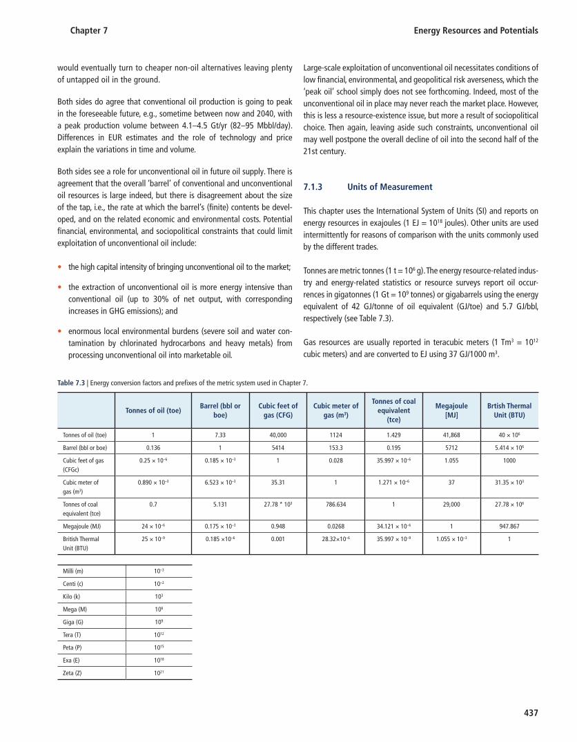
This chapter uses the International System of Units (SI) and reports on energy resources in exajoules (1 EJ = 10 18 joules). Other units are used intermittently for reasons of comparison with the units commonly used by the different trades.
Tonnes are metric tonnes (1 t = 10 6 g). The energy resource-related indus-try and energy-related statistics or resource surveys report oil occur-rences in gigatonnes (1 Gt = 10 9 tonnes) or gigabarrels using the energy equivalent of 42 GJ/tonne of oil equivalent (GJ/toe) and 5.7 GJ/bbl, respectively (see Table 7.3 ).
Gas resources are usually reported in teracubic meters (1 Tm 3 = 10 12 cubic meters) and are converted to EJ using 37 GJ/1000 m 3 .
Table 7.3 | Energy conversion factors and prefi xes of the metric system used in Chapter 7 .
Tonnes of oil (toe)Barrel (bbl or
boe)Cubic feet of
gas (CFG)Cubic meter of
gas (m 3 )
Tonnes of coal equivalent
(tce)
Megajoule [MJ]
Brtish Thermal Unit (BTU)
Tonnes of oil (toe) 1 7.33 40,000 1124 1.429 41,868 40 × 10 6
Barrel (bbl or boe) 0.136 1 5414 153.3 0.195 5712 5.414 × 10 6
Cubic feet of gas (CFGc)
0.25 × 10 –6 0.185 × 10 –3 1 0.028 35.997 × 10 –6 1.055 1000
Cubic meter of gas (m 3 )
0.890 × 10 –3 6.523 × 10 –3 35.31 1 1.271 × 10 –6 37 31.35 × 10 3
Tonnes of coal equivalent (tce)
0.7 5.131 27.78 * 10 3 786.634 1 29,000 27.78 × 10 6
Megajoule (MJ) 24 × 10 –6 0.175 × 10 –3 0.948 0.0268 34.121 × 10 –6 1 947.867
British Thermal Unit (BTU)
25 × 10 –9 0.185 × 10 –6 0.001 28.32 × 10⁻⁶ 35.997 × 10 –9 1.055 × 10 –3 1
Milli (m) 10 –3
Centi (c) 10 –2
Kilo (k) 10 3
Mega (M) 10 6
Giga (G) 10 9
Tera (T) 10 12
Peta (P) 10 15
Exa (E) 10 18
Zeta (Z) 10 21
Energy Resources and Potentials Chapter 7
438
Coal resources are usually accounted for in natural units, although the energy content of coal may vary considerably within and between dif-ferent coal categories. The Bundesanstalt f ü r Geowissenschaften und Rohstoffe (BGR; German Federal Institute for Geosciences and Natural Resources) in Hannover (Germany) is the only institution that converts regional coal occurrences into tonnes of coal equivalent (1 tce = 29.3 GJ). Thus coal resource data comes from the BGR.
Uranium and other nuclear materials are usually reported in tonnes of metal. The thermal energy equivalent of 1 tonne of uranium in average once-through fuel cycles is about 589 terajoules (IPCC, 1996 ).
7.2 Oil
7.2.1 Overview
Oil is one of the most important sources of global energy because of its high energy density, high abundance and easy transportability at stand-ard temperatures and pressures. In 2009, oil was responsible for over one-third (34.8%) of the world’s total primary energy supply. Almost 70% of global oil production is used for transportation and petrochem-istry (IEA, 2010a ).
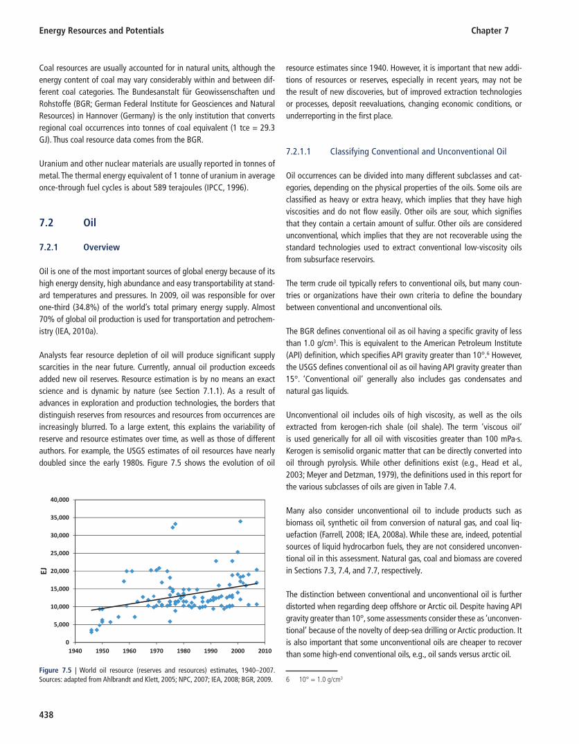
Analysts fear resource depletion of oil will produce significant supply scarcities in the near future. Currently, annual oil production exceeds added new oil reserves. Resource estimation is by no means an exact science and is dynamic by nature (see Section 7.1.1 ). As a result of advances in exploration and production technologies, the borders that distinguish reserves from resources and resources from occurrences are increasingly blurred. To a large extent, this explains the variability of reserve and resource estimates over time, as well as those of different authors. For example, the USGS estimates of oil resources have nearly doubled since the early 1980s. Figure 7.5 shows the evolution of oil
resource estimates since 1940. However, it is important that new addi-tions of resources or reserves, especially in recent years, may not be the result of new discoveries, but of improved extraction technologies or processes, deposit reevaluations, changing economic conditions, or underreporting in the first place.
7.2.1.1 Classifying Conventional and Unconventional Oil
Oil occurrences can be divided into many different subclasses and cat-egories, depending on the physical properties of the oils. Some oils are classified as heavy or extra heavy, which implies that they have high viscosities and do not flow easily. Other oils are sour, which signifies that they contain a certain amount of sulfur. Other oils are considered unconventional, which implies that they are not recoverable using the standard technologies used to extract conventional low-viscosity oils from subsurface reservoirs.
The term crude oil typically refers to conventional oils, but many coun-tries or organizations have their own criteria to define the boundary between conventional and unconventional oils.
The BGR defines conventional oil as oil having a specific gravity of less than 1.0 g/cm 3 . This is equivalent to the American Petroleum Institute (API) definition, which specifies API gravity greater than 10°. 6 However, the USGS defines conventional oil as oil having API gravity greater than 15°. ‘Conventional oil’ generally also includes gas condensates and natural gas liquids.
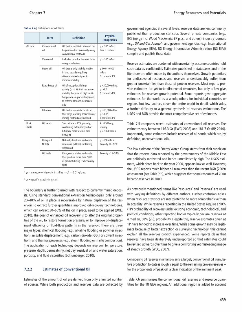
Unconventional oil includes oils of high viscosity, as well as the oils extracted from kerogen-rich shale (oil shale). The term ‘viscous oil’ is used generically for all oil with viscosities greater than 100 mPa·s. Kerogen is semisolid organic matter that can be directly converted into oil through pyrolysis. While other definitions exist (e.g., Head et al., 2003 ; Meyer and Detzman, 1979 ), the definitions used in this report for the various subclasses of oils are given in Table 7.4 .
Many also consider unconventional oil to include products such as biomass oil, synthetic oil from conversion of natural gas, and coal liq-uefaction (Farrell, 2008 ; IEA, 2008a ). While these are, indeed, potential sources of liquid hydrocarbon fuels, they are not considered unconven-tional oil in this assessment. Natural gas, coal and biomass are covered in Sections 7.3 , 7.4 , and 7.7 , respectively.
The distinction between conventional and unconventional oil is further distorted when regarding deep offshore or Arctic oil. Despite having API gravity greater than 10°, some assessments consider these as ‘unconven-tional’ because of the novelty of deep-sea drilling or Arctic production. It is also important that some unconventional oils are cheaper to recover than some high-end conventional oils, e.g., oil sands versus arctic oil.
0
5,000
10,000
15,000
20,000
25,000
30,000
35,000
40,000
1940 1950 1960 1970 1980 1990 2000 2010
EJ
Figure 7.5 | World oil resource (reserves and resources) estimates, 1940–2007. Sources: adapted from Ahlbrandt and Klett, 2005 ; NPC, 2007 ; IEA, 2008 ; BGR, 2009 . 6 10° = 1.0 g/cm 3
Chapter 7 Energy Resources and Potentials
439
The boundary is further blurred with respect to currently mined depos-its. Using standard conventional extraction technologies, only around 20–40% of oil in place is recoverable by natural depletion of the res-ervoir. To extract further quantities, improved oil-recovery technologies, which can extract 30–60% of the oil in place, need to be applied (DOE, 2010 ). The goal of enhanced oil recovery is to alter the original proper-ties of the oil, to restore formation pressure, or to improve oil-displace-ment efficiency or fluid-flow patterns in the reservoir. There are three major types: chemical flooding (e.g., alkaline flooding or polymer injec-tion), miscible displacement (e.g., carbon dioxide [CO 2 ] or solvent injec-tion), and thermal processes (e.g., steam flooding or in situ combustion). The application of each technology depends on reservoir temperature, pressure, depth, permeability, net pay, residual oil and water saturation, porosity, and fluid viscosities (Schlumberger, 2010 ).
7.2.2 Estimates of Conventional Oil
Estimates of the amount of oil are derived from only a limited number of sources. While both production and reserves data are collected by
government agencies at several levels, reserves data are less commonly published than production statistics. Several private companies (e.g., IHS Energy Inc., Wood Mackenzie, BP p.l.c., and others), industry journals (e.g., Oil and Gas Journal ), and government agencies (e.g., International Energy Agency [IEA], US Energy Information Administration [US EIA]) compile and publish these data.
Reserve estimates are burdened with uncertainty as some countries hold such data as confidential. Estimates published in databases and in the literature are often made by the authors themselves. Growth potentials for undiscovered resources and reserves understandably suffer from greater uncertainties than those of proven reserves. Most reports pro-vide estimates for yet-to-be-discovered resources, but only a few give estimates for reserves-growth potential. Some reports give aggregate estimates for the world as a whole, others for individual countries or regions, but few sources cover the entire world in detail, which adds a further difficulty to a general synthesis of reserves estimations. The USGS and BGR provide the most comprehensive set of estimates.
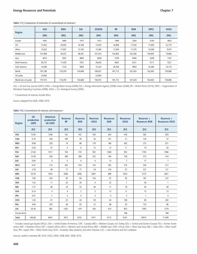
Table 7.5 compares recent estimates of conventional oil reserves. The estimates vary between 116.3 Gt (EWG, 2008 ) and 181.7 Gt (BP, 2010 ). Importantly, some estimates include reserves of oil sands, which are, by definition, unconventional oils.
The low estimate of the Energy Watch Group stems from their suspicion that the reserve data reported by the governments of the Middle East are politically motivated and hence unrealistically high. The USGS esti-mate, which dates back to the year 2000 , appears low as well. However, the USGS reports much higher oil resources than the recent BGR ( 2009 ) assessment (see Table 7.6 ), which suggests that some resources of 2000 became reserves in 2009.
As previously mentioned, terms like ‘resources’ and ‘reserves’ are used with varying definitions by different authors. Further confusion arises when resource statistics are interpreted to be more comprehensive than in actuality. While reserves reporting in the United States require a 90% (1P) probability of recovery under existing economic, technological, and political conditions, other reporting bodies typically declare reserves at a median, 50% (2P), probability. Despite this, reserve estimates given at 1P have tended to increase over time. While some growth may be legiti-mate because of better extraction or surveying technology, this cannot explain all the reserves growth experienced. Some reports claim that reserves have been deliberately underreported so that estimates could be revised upwards over time to give a comforting yet misleading image of steady growth (WEC, 2007 ).
Considering oil reserves in a narrow sense, largely conventional oil, cumula-tive production to date is roughly equal to the remaining proven reserves – for the proponents of ‘peak oil’ a clear indication of the imminent peak.
Table 7.6 summarizes the conventional oil reserves and resource quan-tities for the 18 GEA regions. An additional region is added to account
Table 7.4 | Defi nitions of oil terms.
Term DefinitionPhysical
properties
Oil type Conventional oil
Oil that is mobile in situ and can be produced economically using conventional methods
μ < 100 mPa . s a Low S content
Viscous oil Inclusive term for the next three categories below
μ > 100 mPa . s
Heavy oil Oil that is only slightly mobile in situ, usually requiring stimulation techniques to improve mobility
μ 100–10,000 mPa . s S content <1%
Extra-heavy oil Oil of exceptionally high gravity ( ρ >1.0) that has some mobility because of high in situ temperatures (particularly used to refer to Orinoco, Venezuela oils)
μ <10,000 mPa . s, ρ >1.0 S content >1%
Bitumen Oil that is immobile in situ so that large viscosity reductions or mining methods are needed
μ >10,000 mPa . s ρ >1.0 b S content >1%
Rock strata
Oil sands Sand strata > 25% porosity, containing extra-heavy oil or bitumen, more viscous than heavy oil
k >0.5 Darcy, usually μ > 1000 mPa . s
Heavy-oil NFCRs
Naturally fractured carbonate reservoirs (NFCRs) containing viscous oil
μ >100 mPa . s Porosity 10–20%
Oil shale Kerogenous shales and marls that produce more than 50 l/t of product during Fischer Assay tests
Porosity >15–20%
a μ = measure of viscosity in mPa . s = cP = 0.01 g/cm . s.
b ρ = specifi c gravity in g/cm 3 .
Energy Resources and Potentials Chapter 7
440
Table 7.5 | Comparison of estimates of conventional oil reserves. a
RegionOGJ EWG EIA EXXON BP BGR OPEC USGS
[Mt] [Mt] [Mt] [Mt] [Mt] [Mt] [Mt] [Mt]
Europe 1942 3469 1977 1913 1849 2264 2164 4632
CIS 13,452 20,952 16,784 13,453 16,808 17,543 17,450 22,773
Africa 15,622 17,007 15,192 15,366 17,404 17,276 16,268 9,973
Middle East 101,808 49,252 98,301 101,610 102,803 102,366 100,893 70,866
Asia 4673 7007 4893 4628 5749 5600 5208 7167
North America 28,737 11,429 7921 28,442 8392 6121 5111 5221
Latin America 14,946 7143 9600 15,225 28,706 9854 16,369 10,174
World 181,180 116,259 154,668 180,637 181,712 161,024 163,463 130,806
Oil sands 23,665 23,665
World w/o oil sands 157,515 116,259 154,668 156,972 181,712 161,024 163,463 130,806
OGJ = Oil and Gas Journal ( 2007 ); EWG = Energy Watch Group ( 2008 ); EIA = Energy Information Agency (2008); Exxon ( 2008 ), BP = British Petrol ( 2010 ), OPEC = Organization of Petroleum Exporting Countries (2008), USGS = U.S. Geological Survey ( 2000 ).
a Conventional oil reserves include NGLs.
Source: adapted from BGR, 2009 ; 2010 .
Table 7.6 | Conventional oil reserves and resources. a
Region
Oil production
2009
Historical production
till 2009
Reserves BP
Reserves BGR
Reserves USGS
Resources BGR
Resources USGS
Reserves + Resources BGR
Reserves + Resources USGS
[EJ] [EJ] [EJ] [EJ] [EJ] [EJ] [EJ] [EJ] [EJ]
USA 15.00 1246 162 162 183 420 476 582 659
CAN 6.70 200 189 28 36 101 21 129 57
WEU 8.98 329 74 88 179 186 492 275 671
EEU 0.28 47 4 6 15 13 11 19 26
FSU 27.64 1017 704 735 953 1008 952 1743 1906
NAF 10.38 336 389 388 252 184 158 573 410
EAF 0.00 0 0 4 0 13 7 17 7
WCA 6.07 214 263 254 142 302 375 556 517
SAF 3.78 48 77 77 24 150 97 227 121
MEE 50.78 1823 4308 4286 2967 889 1654 5175 4621
CHN 7.90 220 85 84 142 97 95 181 237
OEA 1.02 11 26 26 0 32 1 58 1
IND 1.57 46 33 33 40 17 18 50 58
OSA 0.14 4 4 2 3 13 11 15 13
JPN 0.01 2 0 0 0 0 0 1 0
OCN 1.20 41 25 24 94 44 108 69 202
PAS 4.90 203 68 65 22 88 63 153 86
LAC 20.30 862 1203 479 426 614 853 1093 1279
Circum-Arctic 768 768
Total 166.68 6647 7615 6742 5477 4172 6161 10914 11,638
a Includes natural gas liquids (NGLs). USA = United States of America; CAN - Canada; WEU = Western Europe, incl. Turkey; EEU = Central and Eastern Europe; FSU = Former Soviet Union; NAF = Northern Africa; EAF = Eastern Africa; WCA = Western and Central Africa; MEE = Middle East; CHN =China; OEA = Other East Asia; IND = India; OSA = Other South Asia; JPN =Japan; PAS = Other Pacifi c Asia; OCN = Australia, New Zealand, and other Oceania; LAC = Latin America and the Caribbean
Sources: author’s estimate; BP, 2010 ; USGS, 2000 ; 2008 ; BGR, 2009 ; 2010 .

Chapter 7 Energy Resources and Potentials
441
for resources located within the Arctic Circle (USGS, 2008 ). The table compiles reserves estimates from BP, BGR, and the USGS – the three organizations that regularly assess global oil reserves or resources. While reserve estimates exhibit only slight variance, less than 15% between the highest (7615 EJ by BP) and lowest estimates (6635 EJ by BGR), resource estimates show almost a 50% difference (4170 EJ by BGR and 6150 EJ by USGS).
The discrepancies arise because of different definitions, boundaries, and classifications of different oil types. While reserves estimation is somewhat better defined, resource estimation has very few guidelines and is thus subject to greater institutional subjectivity. For example, the USGS resource estimate includes oil occurrences in the Arctic (768 EJ). Furthermore, estimates of resources in undiscovered fields, despite their inherent ambiguity, have also grown over time. This is mainly because technology changes that have either shifted resources from the uncon-ventional to conventional category, or have opened new territories to exploration (e.g., deep-water areas).
Figure 7.6 displays the regional distribution of conventional oil reserves and resources. Almost two-thirds of global conventional oil is shared between the Middle Eastern countries (48.6%) and the Former Soviet Union (FSU) (16.7%), while the remaining regions, except Latin America (9.0%) and the United States (5.7%) hold less than 5% (BGR, 2009 ).
The regional distribution of oil resources has significant implications for rapidly developing economies such as China and India. China’s ability to provide for its own needs is limited because its proven oil reserves are small compared to its consumption. Despite recent attempts at
diversifying its oil supply, China will inevitably become more dependent on Middle Eastern oil to fuel its economic development.
7.2.3 Types of Unconventional Oil
7.2.3.1 Viscous Oil
Anaerobic biodegradation of light oil is recognized as the main process responsible for the large viscous oil deposits around the world (Atlas and Bartha, 1992 ; Head et al., 2003 ). Aitken et al. ( 2004 ) investigated the hydrocarbon degradation of 77 oil samples from around the world, including Canadian tar sands deposits, and concluded that the hydro-carbon biodegradation must have been an anaerobic process, at least at some point, and this is certainly the case for viscous oil deposits at depths where aerobic biodegradation was unlikely. Thus, light oil gen-erated deep in megasynclinal structures migrated up-dip because of density differences and hydrodynamic forces until geochemical condi-tions suitable for biodegradation were encountered. Archaeobacteria then fed on the light oil, generating viscous oil and CH 4 . Furthermore, at shallow depths, some aerobic effects may occur, and light-oil fractions can also be removed by hydrodynamic washing and diffusion, further increasing the viscosity. As a result of increasing temperature and the biodegradation origins of viscous oil, it is rarely found below depths of ~2000 m; probably greater than 85% of the resource base is shallower than 1000 m ( Figure 7.7 ).
Many of the molecules of high molecular weight, such as asphaltenes, that give the oil its high viscosity are the remnants of the cell walls (lipids) of the bioorganisms. The oil contains sulfur, as well as heavy
0
1000
2000
3000
4000
5000
6000
0
20
40
60
80
100
120
140
MEE
FSU
LAC
USA
NA
F
WCA
WEU
CHN
PAS
CAN
SAF
OCN IN
D
OEA EEU
OSA EA
F
JPN
EJ
Conv
en�
onal
oil
rese
rves
and
reso
urce
s G
t
Figure 7.6 | Regional distribution of conventional oil reserves and resources. Source: BGR, 2010 .

Energy Resources and Potentials Chapter 7
442
metals such as vanadium and nickel. The concentration of these elem-ents in viscous oil is a function of density: oils of ρ >1.0 can have sulfur concentrations greater than 4% and heavy metal contents as high as 500 parts per million (ppm). Viscous oils with ρ <0.92–0.93, by contrast, typically have less than 25% of such concentrations. In the production of these resources, the elements S, V, Ni, Fe, and the high oil viscosity lead to problems in processing and environmental management (Head et al., 2003 ).
Bitumen is the heaviest, thickest form of petroleum. The bitumen con-tained in shallow oil (tar) sands can be recovered using surface min-ing techniques. However, it takes about two tonnes of oil sands mined (0.9 m 3 ) and processed to obtain one barrel of synthetic crude oil. About 90% of mined bitumen can be recovered by way of hot water and sur-factant mixing and separation from the sand in special agitation-flo-tation tanks. After oil extraction, solids and water are returned to the mine, which is eventually reclaimed. Separated bitumen is then shipped or upgraded to synthetic crude oil.
Deposits with overburdens of more than perhaps 60 m must be exploited by in situ methods, e.g., injecting steam into the depos-its to reduce the bitumen’s viscosity and increase reservoir pressure (which also induces fracturing), and thereby enable bitumen to flow (Dusseault, 2002 ). The advantage of in situ extraction is avoidance of
the massive movement of the oil’s host material and attendant surface disruption. The disadvantage is its water and energy intensity (about 3–4 barrels of steam per barrel of oil produced). Two processes are cur-rently applied: cyclic steam simulation (CSS) (Nasr and Ayodele, 2005 ) and steam-assisted gravity drainage (SAGD) (Butler and Stephens, 1980 ; 1981 ). CSS involves the injection of a charge of high-pressure steam into a well over some time, and during the production cycle the heat and pressure mobilize bitumen flow to the same well, along with hot water. The cycle is repeated when the rate of production flow declines and a well may have a lifespan of 8–12 years. SAGD involves twin parallel horizontal wells separated vertically by about 4–5 m. Steam is injected into the top well, the mobilized bitumen drains into the bottom well and is lifted to the surface. Other in situ extraction processes being tested include the use of chemical solvents, electric heating, and partial combustion, none of which are currently consid-ered commercially viable.
In situ production of heavy and extra-heavy oils utilizes methods simi-lar to those for the production of oil sands, except that if the viscosity is modest and the permeability high, conventional pumping and water flooding may result in modest recovery factors (5–20%) without steam stimulation. If the sand is unconsolidated and has good solution-gas content, in many cases encouraging sand influx has proven to be a via-ble and economic production process.
Figure 7.7 | The ‘standard’ model for viscous oil formation. Source: Head et al., 2003 .

Chapter 7 Energy Resources and Potentials
443
Not only are viscous oils difficult to extract, they are difficult to process and transport. These oils may be viewed as deficient in hydrogen (carbon rich) and must be upgraded to produce useful products. Hydrogenation and carbon rejection (coking) are used to improve the hydrogen-to- carbon ratio, with CH 4 used as the source of hydrogen during upgrading. The heavy metals lead to difficulties in processing because they rapidly poison catalyst beds. Large volumes of sulfur and coke are by-products of typical upgrading operations. Once upgraded, the synthetic crude oil is sent to conventional refineries for further beneficiation to create mar-ketable products. If local upgrading is not used, pipelining viscous oil requires blending with diluents, light oil, or synthetic crude oil.
At the present time (2010), only nine countries in the world produce more than 250,000 bbl/day or 12.5 Mt/yr of non-conventional (vis-cous) oil: Canada (~90 Mt/yr), Venezuela (~50 Mt/yr), the United States (~20 Mt/yr), Mexico (~18 Mt/yr), and each of Russia, China, Oman, Iran, and Brazil at about 15 Mt/yr.
7.2.3.2 Oil Shales (Kerogen)
Kerogen is a semisolid organic compound formed from algal residues. It is found in shales – sedimentary rocks that were buried rapidly, which led to low oxygen conditions that preserved the lipids and other similar cellu-lar debris from the algae. Over geological time, kerogen buried to depths greater than 3 km and at temperatures greater than 80–90ºC is bro-ken down and converted into light oil. Economically interesting kerogen deposits are found at relatively shallow depths, less than 1500–2000 m. Kerogen in oil shales is viewed as ‘immature oil’ and, like viscous oil, is deficient in hydrogen (Dyni, 2006 ; Altun et al., 2006 ; WEC, 2007 ).
Near-surface deposits can be produced with standard surface and underground mining techniques using surface retorting (pyrolysis),
and the shale-oil product (a mixture of gases and liquids) used directly as boiler fuel or as hydrocarbon products. The generation of synthetic crude oil from kerogen requires pyrolytic retorting with collection and treatment of the product. In contrast to most viscous oil, kerogen in deeper reservoirs cannot be mobilized, but must be converted physic-ally through pyrolytic approaches. For example, kerogenous shale can be exposed to a combustion process (oxypyrolysis) that literally cooks the shale by partial combustion, generating valuable lighter products.
In situ or surface anoxic pyrolysis requires temperatures greater than 325°C to decompose the complex molecules into liquid and gaseous products that can be recovered, leaving behind perhaps 30% of the organic matter as elemental carbon. Anoxic in situ extraction tech-nologies are based on conductive heating of shale beds using thermal energy (electrical heating or hot fluid circulation), with separate wells to collect generated fluids (e.g., Biglarbigi et al., 2009 ; Crawford et al., 2008 , 2009 ).
Unlike heavy oil, kerogen does not contain sulfur and heavy metals. Thus, the products from pyrolysis are light ‘sweet’ gases and liquids that are processed relatively easily.
7.2.4 Estimates of Unconventional Oil
There are about 1780 Gt (74.8 ZJ) of liquid petroleum (shale oil, heavy oil, extra-heavy oil, and bitumen) trapped in sedimentary rocks in several thou-sand basins around the world ( Table 7.7 ). Oil-shale resources are estimated at about 382–450 Gt (16–18.9 ZJ) (Dyni, 2006 ; WEC, 2007 ). However, these figures, particularly for oil shale, are somewhat conservative because of the lack of detailed exploration for these resources, particularly in coun-tries with large conventional oil resources. For example, Libya, Iraq, Saudi Arabia, Iran, Oman, Kuwait, the United Arab Emirates, and other countries
Table 7.7 | World oil resource estimates.
Oil type Definition Gt ZJ
Conventional Original oil <100 cP viscosity in place, including sandstones and carbonates 614 25.7
Produced to date Estimated cumulative production to date, 98% of which has been conventional oil <100 cP in situ
150–164 6.3–6.9
Remaining conventional Total remaining in place Technically recoverable, current technology Ultimately recoverable, including above
464 150 205
19.4 6.3 8.6
Viscous oil Original oil in place, all rock types 1350 56.4
Viscous oil in sandstones All viscous oil in sandstone reservoirs Technically recoverable, current technology Ultimately recoverable, including above
~1023 109 273
42.8 4.6 11.4
Viscous oil in NFCRs All viscous oil in NFCRs Technically recoverable, current technology Ultimately recoverable, including above
205–300 <14 41
8.6–12.5 <0.59
1.7
Shale oil converted into liquid oil (excluding gas) Estimated barrels in place, >50 l/t shale oil Technically recoverable, current technology Ultimately recoverable, including above
382–450 <14 41
16–18.8 <0.59
1.7
Sources: quantitative data from authors’ estimates; WEC, 2007 ; USGS, 2000 ; 2008 ; IEA, 2008a ; BGR, 2009 .
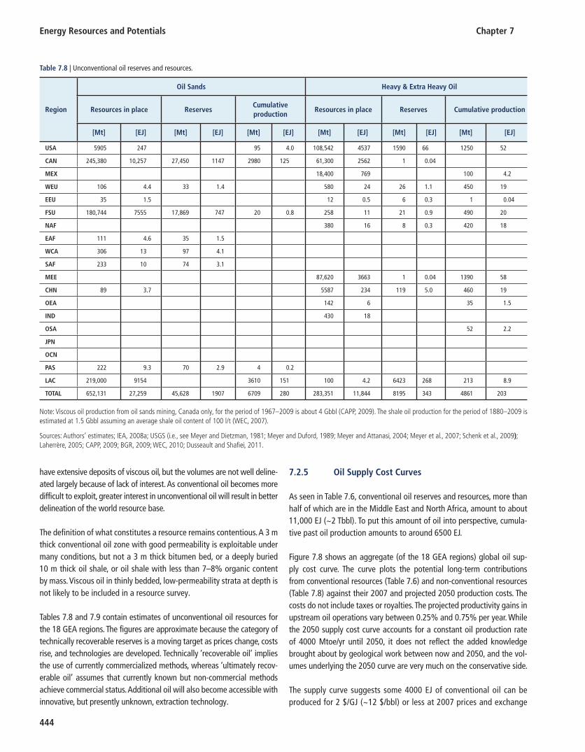
Energy Resources and Potentials Chapter 7
444
have extensive deposits of viscous oil, but the volumes are not well deline-ated largely because of lack of interest. As conventional oil becomes more difficult to exploit, greater interest in unconventional oil will result in better delineation of the world resource base.
The definition of what constitutes a resource remains contentious. A 3 m thick conventional oil zone with good permeability is exploitable under many conditions, but not a 3 m thick bitumen bed, or a deeply buried 10 m thick oil shale, or oil shale with less than 7–8% organic content by mass. Viscous oil in thinly bedded, low-permeability strata at depth is not likely to be included in a resource survey.
Tables 7.8 and 7.9 contain estimates of unconventional oil resources for the 18 GEA regions. The figures are approximate because the category of technically recoverable reserves is a moving target as prices change, costs rise, and technologies are developed. Technically ‘recoverable oil’ implies the use of currently commercialized methods, whereas ‘ultimately recov-erable oil’ assumes that currently known but non-commercial methods achieve commercial status. Additional oil will also become accessible with innovative, but presently unknown, extraction technology.
7.2.5 Oil Supply Cost Curves
As seen in Table 7.6 , conventional oil reserves and resources, more than half of which are in the Middle East and North Africa, amount to about 11,000 EJ (~2 Tbbl). To put this amount of oil into perspective, cumula-tive past oil production amounts to around 6500 EJ.
Figure 7.8 shows an aggregate (of the 18 GEA regions) global oil sup-ply cost curve. The curve plots the potential long-term contributions from conventional resources ( Table 7.6 ) and non-conventional resources ( Table 7.8 ) against their 2007 and projected 2050 production costs. The costs do not include taxes or royalties. The projected productivity gains in upstream oil operations vary between 0.25% and 0.75% per year. While the 2050 supply cost curve accounts for a constant oil production rate of 4000 Mtoe/yr until 2050, it does not reflect the added knowledge brought about by geological work between now and 2050, and the vol-umes underlying the 2050 curve are very much on the conservative side.
The supply curve suggests some 4000 EJ of conventional oil can be produced for 2 $/GJ (~12 $/bbl) or less at 2007 prices and exchange
Table 7.8 | Unconventional oil reserves and resources.
Region
Oil Sands Heavy & Extra Heavy Oil
Resources in place ReservesCumulative production
Resources in place Reserves Cumulative production
[Mt] [EJ] [Mt] [EJ] [Mt] [EJ] [Mt] [EJ] [Mt] [EJ] [Mt] [EJ]
USA 5905 247 95 4.0 108,542 4537 1590 66 1250 52
CAN 245,380 10,257 27,450 1147 2980 125 61,300 2562 1 0.04
MEX 18,400 769 100 4.2
WEU 106 4.4 33 1.4 580 24 26 1.1 450 19
EEU 35 1.5 12 0.5 6 0.3 1 0.04
FSU 180,744 7555 17,869 747 20 0.8 258 11 21 0.9 490 20
NAF 380 16 8 0.3 420 18
EAF 111 4.6 35 1.5
WCA 306 13 97 4.1
SAF 233 10 74 3.1
MEE 87,620 3663 1 0.04 1390 58
CHN 89 3.7 5587 234 119 5.0 460 19
OEA 142 6 35 1.5
IND 430 18
OSA 52 2.2
JPN
OCN
PAS 222 9.3 70 2.9 4 0.2
LAC 219,000 9154 3610 151 100 4.2 6423 268 213 8.9
TOTAL 652,131 27,259 45,628 1907 6709 280 283,351 11,844 8195 343 4861 203
Note: Viscous oil production from oil sands mining, Canada only, for the period of 1967–2009 is about 4 Gbbl (CAPP, 2009 ). The shale oil production for the period of 1880–2009 is estimated at 1.5 Gbbl assuming an average shale oil content of 100 l/t (WEC, 2007 ).
Sources: Authors’ estimates; IEA, 2008a ; USGS (i.e., see Meyer and Dietzman, 1981 ; Meyer and Duford, 1989 ; Meyer and Attanasi, 2004 ; Meyer et al., 2007 ; Schenk et al., 2009 ) ; Laherr è re, 2005 ; CAPP, 2009 ; BGR, 2009 ; WEC, 2010 ; Dusseault and Shafi ei, 2011 .
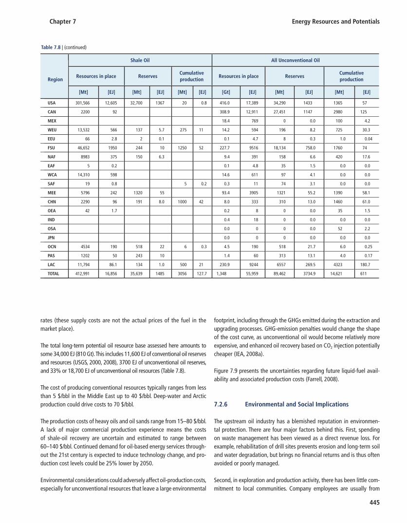
Chapter 7 Energy Resources and Potentials
445
rates (these supply costs are not the actual prices of the fuel in the market place).
The total long-term potential oil resource base assessed here amounts to some 34,000 EJ (810 Gt). This includes 11,600 EJ of conventional oil reserves and resources (USGS, 2000 , 2008 ), 3700 EJ of unconventional oil reserves, and 33% or 18,700 EJ of unconventional oil resources ( Table 7.8 ).
The cost of producing conventional resources typically ranges from less than 5 $/bbl in the Middle East up to 40 $/bbl. Deep-water and Arctic production could drive costs to 70 $/bbl.
The production costs of heavy oils and oil sands range from 15–80 $/bbl. A lack of major commercial production experience means the costs of shale-oil recovery are uncertain and estimated to range between 60–140 $/bbl. Continued demand for oil-based energy services through-out the 21st century is expected to induce technology change, and pro-duction cost levels could be 25% lower by 2050.
Environmental considerations could adversely affect oil-production costs, especially for unconventional resources that leave a large environmental
footprint, including through the GHGs emitted during the extraction and upgrading processes. GHG-emission penalties would change the shape of the cost curve, as unconventional oil would become relatively more expensive, and enhanced oil recovery based on CO 2 injection potentially cheaper (IEA, 2008a ).
Figure 7.9 presents the uncertainties regarding future liquid-fuel avail-ability and associated production costs (Farrell, 2008 ).
7.2.6 Environmental and Social Implications
The upstream oil industry has a blemished reputation in environmen-tal protection. There are four major factors behind this. First, spending on waste management has been viewed as a direct revenue loss. For example, rehabilitation of drill sites prevents erosion and long-term soil and water degradation, but brings no financial returns and is thus often avoided or poorly managed.
Second, in exploration and production activity, there has been little com-mitment to local communities. Company employees are usually from
Shale Oil
Resources in place ReservesCumulative production
[Mt] [EJ] [Mt] [EJ] [Mt] [EJ]
301,566 12,605 32,700 1367 20 0.8
2200 92
13,532 566 137 5.7 275 11
66 2.8 2 0.1
46,652 1950 244 10 1250 52
8983 375 150 6.3
5 0.2
14,310 598
19 0.8 5 0.2
5796 242 1320 55
2290 96 191 8.0 1000 42
42 1.7
4534 190 518 22 6 0.3
1202 50 243 10
11,794 86.1 134 1.0 500 21
412,991 16,856 35,639 1485 3056 127.7
All Unconventional Oil
Resources in place ReservesCumulative production
[Gt] [EJ] [Mt] [EJ] [Mt] [EJ]
416.0 17,389 34,290 1433 1365 57
308.9 12,911 27,451 1147 2980 125
18.4 769 0 0.0 100 4.2
14.2 594 196 8.2 725 30.3
0.1 4.7 8 0.3 1.0 0.04
227.7 9516 18,134 758.0 1760 74
9.4 391 158 6.6 420 17.6
0.1 4.8 35 1.5 0.0 0.0
14.6 611 97 4.1 0.0 0.0
0.3 11 74 3.1 0.0 0.0
93.4 3905 1321 55.2 1390 58.1
8.0 333 310 13.0 1460 61.0
0.2 8 0 0.0 35 1.5
0.4 18 0 0.0 0.0 0.0
0.0 0 0 0.0 52 2.2
0.0 0 0 0.0 0.0 0.0
4.5 190 518 21.7 6.0 0.25
1.4 60 313 13.1 4.0 0.17
230.9 9244 6557 269.5 4323 180.7
1,348 55,959 89,462 3734.9 14,621 611
Table 7.8 | (continued)
Region
USA
CAN
MEX
WEU
EEU
FSU
NAF
EAF
WCA
SAF
MEE
CHN
OEA
IND
OSA
JPN
OCN
PAS
LAC
TOTAL

446
Tabl
e 7.
9 | U
ncon
vent
iona
l oil
rese
rves
and
reso
urce
s.
Regi
on
Oil
sand
sH
eavy
& e
xtra
hea
vy o
ilSh
ale
oil
All
unco
nven
tion
al o
il
Am
ount
in
pla
ceRe
sour
ces
Rese
rves
Am
ount
in
plac
eRe
sour
ces
Rese
rves
Am
ount
in
plac
eRe
sour
ces
Rese
rves
Am
ount
in
plac
eRe
sour
ces
Rese
rves
[Mt]
[Mt]
[Mt]
[Mt]
[Mt]
[Mt]
[Mt]
[Mt]
[Mt]
[EJ]
[EJ]
[EJ]
USA
59
0520
650
415
763
301,
566
73,0
3035
,970
12,8
7031
4215
04
CAN
27
2,00
081
,853
27,4
500
21
2200
00
11,4
6234
2211
47
WEU
33
610
633
2312
419
2613
,532
307
151
676
359
EEU
10
035
061
126
664
29
20
FSU
18
0,74
457
,005
17,8
6914
3425
821
46,6
5254
526
895
6524
1675
9
NA
F 0
00
7914
889
8333
516
537
915
7
EAF
352
111
350
00
50
015
51
WCA
97
130
697
00
014
,310
00
639
134
SAF
739
233
740
00
190
032
103
MEE
0
00
10
157
9629
4814
5224
212
361
CHN
25
389
014
1125
411
922
9042
721
016
532
14
OEA
0
00
00
042
00
20
0
IND
0
00
00
00
00
00
0
OSA
0
00
00
00
00
00
0
JPN
0
00
00
00
00
00
0
OCN
0
00
00
045
3411
5656
919
048
24
PAS
708
222
700
00
1202
543
267
8032
14
LAC
260
920
240,
740
46,8
2064
2311
,794
298
147
10,5
6719
7327
5
TOTA
L 46
2,36
814
2,11
745
,628
246,
453
47,8
5566
0841
2,99
179
,592
39,2
0246
,892
11,2
6838
22
Sour
ce: B
GR,
200
9 .

Chapter 7 Energy Resources and Potentials
447
distant communities, spending a limited time in the area. Again, drill-site rehabilitation serves as a useful example. In Wytch Farm (UK), only a few kilometers from expensive beach properties, drill sites are fully reha-bilitated, reforested, and invisible from all recreational sites. However, in southeastern Ecuador, 30-year-old drill sites in the jungle, including drilling waste pits and oil spills, continue to erode and cause silting and local contamination (San Sebastian et al., 2001).
Third, there is the joint problem of poor regulatory enforcement and occasionally associated corruption. Environmental protection requires strong, transparent, and consistent enforcement of regulatory guide-lines, often in remote areas. Human fallibility and greed, combined with industry ‘capture’ of regulatory bodies, has led to unfortunate cases of collusion and corruption, invariably with negative consequences. Neutral third-party annual audits with full publication of results constitute an approach to reducing this problem.
Fourth, ignorance of environmental impacts has led to a general reactive attitude to environmental management rather than to proactive avoid-ance. Once a severe problem happens, mitigation costs and reputational loss often far exceed the initial investment in avoidance that should have been made. Increasing corporate attention to employee education is reducing this problem.
Recent and continued progress (Marika et al. 2009 ) suggests that goals of ‘minimal impact-quasi zero emissions’ are technically feasible and economically attainable, as well as socially desirable.
7.2.6.1 Environmental Issues in Oil Development
Oil development involves, among others, the following activities: seismic exploration, exploratory and development drilling, infrastructure generation,
0
5
10
15
20
25
30
0 5000 10000 15000 20000 25000 30000 35000
Prod
uc�
on c
osts
, $/G
J
EJ
Current Technology
2050 Technology
Figure 7.8 | Long-term oil supply curve 7 – combined global conventional and uncon-ventional oil reserves and resources. Source: USGS, 2000 ; 2008 ; IEA, 2008a ; Deutsche Bank, 2009 ; Aguilera et al., 2009 .
20
60
40
80
100
- -4 000 0 4 000 8 000 12 000 16 000 20 000 24 000 28 000 32 000 36 000
Prod
uc�
on c
ost (
2005
$ p
er b
bl)
Reserves and Resources (EJ)
Conven�onalOil
EOR
Tar sands andheavy oil
Oil shaleYet to be producedAlreadyproduced
-8 000
Figure 7.9 | Liquid fuel supply potentials and production costs. The green bars represent the economic cost of extracting fuels. The black bar to the left of the vertical axis represents cumulative past oil production (about 157 Gt). The height of the bars represents the degree of uncertainty of the production costs. The widths of the bars represent how plentiful the resource is, and the lightness of the bars refl ects the degree of uncertainty of resource availability. Source: adapted from Farrell, 2008 .
7 The 2050 supply curve is net of a hypothetical cumulative production between 2005 and 2050 based on the historically observed production growth rate between 1995 and 2007. The resources exploited during the period up to 2050 are no longer available after 2050. Despite upstream innovation and technology change, the 2050 supply cost curve is higher as resource extraction until 2050 is expected to exploit lower cost occurrences fi rst.
Energy Resources and Potentials Chapter 7
448
long-term production, transportation (generally pipelines), siting for large upgrading, refining and petrochemical facilities, and postactivity cleanup.
Current liabilities that reside in previously contaminated sites are large, as the industry efforts to rectify the impact of poor historical practices. The full economic implications of poor environmental management is little understood and under heated debate. While issues common to oil and gas development are discussed in this section in a somewhat posi-tive light, with the notion that the industry is doing better, it is clear that it can and must continue to improve.
With regard to climate-change issues, the major CO 2 emissions related to oil products come from their end-use combustion, and these numbers overwhelm the emissions from oil exploration and production activity (Charpentier et al., 2009 ; IHS-CERA, 2010 ).
However, there are other major impacts on land and water resources. Seismic work requires access to land areas, generally by cutting paths to allow the use of all-terrain vehicles. Sensitive areas include permafrost regions, forests, and steep terrain where vegetation disturbance leads to permafrost degradation or soil erosion. Low-impact methods reduce damage in these areas by hand-cutting narrow lines, and using helicop-ters and vehicles with small contact pressure for transport.
Exploratory drilling with light helicopter rigs has reduced road-triggered erosion, and better cuttings and waste-disposal practices, combined with improved site rehabilitation, have significantly reduced waste abandon-ment and erosion. Directional pad drilling in the North Slope of Alaska and winter-only transport have reduced the surface area needs to about 13%, compared to 30 years ago. Similar improvements have been made in jungle areas (Peru) and in farming regions (Saskatchewan and Alberta). Fossil-fuel exploitation can be compatible with agriculture and sensitive ecosystems.
Vast volumes of produced water (greater than three tonnes of water per tonne of oil worldwide) are now systematically reinjected for water flooding or disposed into deep saline aquifers (Veil and Quinn, 2008 ). In development plans for the Mara ñ on Basin in Peru, companies are contractually committed to full reinjection without diversion to river courses. Landfills should be avoided for any solid waste that contains species potentially harmful to subsurface potable water because of long-term security issues: all landfills leak or will eventually leak. Other produced liquid wastes, emulsions, and solid wastes can be slurried and reinjected safely, virtually to eliminate environmental liability. After exploitation and beneficiation, sites and spills must be properly cleaned and disposed, and corporations are requested more and more to post bonds (insurance) against future problems. Cleanup must be an ongoing and regulated activity, not reserved for when production is fully terminated.
Pipeline and flowline installations in jungle areas now increasingly use forest canopy preservation, and the Aleyska pipeline from the Alaska
North Slope lies largely on elevated beams placed on thermo-siphon piles that do not degrade the permafrost. In built-up areas, pipeline burial, and reuse of rights-of-way as farmland is the rule, and pipe-line companies have trained response teams for accident manage-ment. Aggressive reseeding of cleared areas using rapidly growing grasses and plants reduces erosion, and in many areas actually pro-vides enhanced grazing for ungulates. Forty years ago all these prac-tices only took place in developed areas; now they are basically the rule everywhere, but regulatory vigilance is vital. In particular, as the pipeline infrastructure ages, better inspections and corrosion-detection methods are needed to identify problems before they become breaks and spills (OGJ, 2010 ).
Environmental difficulties at large processing centers attract a great deal of media attention, which forces operators to become more vigilant and proactive. Nevertheless, a long history of site contamination blights the reputation of fossil-fuel companies. Many sites around the United States and the Mexico Gulf Coast are in a state of severe contamination (hydrocarbons, chlorinated hydrocarbons, and heavy metals); in some cases, sites (and responsibilities) have been abandoned for several dec-ades. Deep slurried solids injection provides a method for cleaning these and other sites.
During offshore developments, the key to protecting marine environ-ments near production and exploration activities is to plan and enforce zero liquid and solid discharge policies, as adopted by the Government of Norway, for example (Ekins et al., 2007 ). This is achieved by shipping waste to shore for treatment and by the injection of solids and liquid waste into oil-free saline aquifers. Spill risks must be managed properly and emergency response measures put in place. Old platforms are sal-vaged or sunk to provide rich environments for marine life, as iron is a limited nutrient in the ocean.
The recent (April 2010 ) Deep Water Horizon blowout in the Gulf of Mexico is having profound effects on safety practices, both to prevent and to respond to such incidents (OGJ, 2010 ). At the present time opera-tors in the region have invested large sums to create a joint industry-response approach, and regulatory aspects are being examined carefully. This accident will affect all future offshore practices, and the cost to BP (US$40 billion projected is the most recent estimate) has already trig-gered improvements in procedures manuals, operational quality control, regulatory management, and response plans. These changes will reduce environmental risk for offshore operations around the world.
7.2.6.2 Oil Sands Mining In Canadian surface mining of viscous oil, the issues are atmospheric emissions (sulfoxides [SO x ], nitrogen oxides [NO x ], CO 2 , and particu-lates), water use (water sources, tailings ponds, seepage into groundwa-ter), and solid-waste management (sand-tailings management, mature fine-grained oily sludges, long-term coke and sulfur storage, disposal of solid wastes such as pipe scale, tank bottoms, and emulsions). Concerns over massive surface changes can be mitigated through reclamation

Chapter 7 Energy Resources and Potentials
449
efforts with the resultant terrain often more ecologically productive than before. Furthermore, the area amenable to surface mining in Alberta, about 3400 km 2 , is no larger than 60% of the greater Los Angeles area; 95% of Alberta’s boreal forests will remain unaffected (~470 km 2 of boreal forest has been cleared or mined to date).
One cubic meter of ore weighs 2.2 tonnes and averages 0.68 m 3 of silica sand, 0.23 m 3 of oil, 0.06 m 3 of water, and 0.03 m 3 of fine-grained silt and clay. The products are approximately 0.2 m 3 (0.171 t) of raw bitu-men, 1.1 m 3 of bulked sand (35% porosity) that contains water, fine-grained minerals, and residual oil in the pores, 1.6 m 3 of water, much of which is recycled for further extraction, and 0.20 m 3 of oily aqueous sludge containing 60% of the clay minerals in the original raw ore. In addition, for each cubic meter of ore, 0.3 m 3 of overburden is removed, organic soil is stored for future reclamation, and 0.01 m 3 each of coke and sulfur are produced and stockpiled. CO 2 emissions for mining and upgrading are about 700–750 kgCO 2 per tonne of oil, exclusive of trans-portation and further refining (IHS CERA, 2011 ).
Of these materials, the large volumes of pond sludge constitute the major waste stream that presents a significant long-term problem, although tailings dams, coke, and sulfur may have local groundwater impacts. Since mining of oil sand in Alberta began 40 years ago, the volumes of sludge per barrel of bitumen produced have halved, and research continues to develop less water-intensive extraction methods. General groundwater drainage toward the large local river (Athabasca) means that management of contamination is feasible through intercep-tion and dilution. The recent focus of industry on sludge rehabilitation has resulted in large-scale experiments by corporations (Shell, Suncor, Syncrude) into methods to reduce sludge generation volumes and solid-ify the remaining sludge.
The incentive arises from a tightening of licensing practices by the Alberta government, but progress remains slow. Some low-volume, difficult wastes are also being disposed into deep salt caverns (e.g., Veil et al., 1999 ) in Alberta and Saskatchewan to achieve permanent isolation. Nevertheless, final pond closure, elimination of mature fine-grained tailings sludge, and reestablishing a stable productive landscape represent challenges to be met.
Recovery processes for in situ viscous oil Steam for heavy oil recovery requires heat and water sources, as well as water recycling. Natural gas is by far the main source of heat, but asphaltene and coke (or coal) combustion for heat and H 2 generation will become more common. On average, recovery of one tonne of vis-cous oil by steam methods requires three tonnes of water as steam at 200–300°C. Steam generation requires water treatment and attendant sludge-disposal needs. Production of viscous oil also generates emul-sions that are challenging to treat and are best disposed of through deep injection. Saline boiler subfeed water and other contaminated water can be injected, along with all other contaminated water, into saline aquifers. CO 2 emissions (extraction, upgrading, transportation, and refining only) are 990–1100 kg/t of oil for SAGD methods, and
1170–1390 kg/tCO 2 per tonne oil for cyclic steam stimulation (IHS CERA 2010). About 85% of emissions are allocated to steam generation, H 2 generation, power, and pumping inputs, ranked by size. For comparison, synthetic crude oil from mining requires about 950–1000 kg/tCO 2 to bring the product from the ground to the service station.
In situ combustion processes, by contrast, are anhydrous; CO 2 emissions are estimated at 880–1000 kg/t, generally less than steam projects based on natural gas. Furthermore, lack of significant liquid and solid wastes make in situ combustion processes more benign in terms of envi-ronmental impact. However, combustion methods remain far from com-mercialization at this time.
Oil-shale development Anoxic in situ pyrolysis of oil shales at high temperatures generates no surface wastes or significant atmospheric emissions. Anoxic surface pyrolysis is also a process with low atmospheric emissions, but solid wastes are generated. If combustion-based in situ pyrolysis or surface retorting is used, CO 2 emissions are likely to be about 1170–1470 kg/t, not counting additional energy sources for heating or transportation. If ore is mined and retorted, spent shale to be disposed of has a vol-ume bulking factor of about 20%, but it is an inert substance without residual oil or environmentally damaging substances. In the vast oil-shale deposits in the United States, as well as for some other oil-shale deposits in Jordan, China, and Australia, an arid climate means that reclamation of mined land is challenging, although the land-use value of these arid regions is low. Water requirements for oil-shale develop-ment are low because steam will not be used and retorting is anhy-drous. It is unlikely that large-scale exploitation of the vast American oil-shale deposits will ever occur by surface mining methods because of the environmental impacts, solids management costs, and reclama-tion problems.
Zero emissions targets Suppressing stack emissions of SO x , NO x , and particulates to near-zero levels is currently achievable, but CO 2 emissions will remain an envi-ronmental concern for the foreseeable future (see also Chapters 12 and 13 ). Produced solids, scale, cuttings, pond sludges, tank bottoms, emulsions, and treatment fluids, as well as many other noxious and hazardous wastes, can be slurried with untreated waste water and dis-posed of safely through deep-well injection. The slurry is injected at depths greater than 400 m into saline aquifers with adequate seals against upward flow. Solids are permanently retained in the stratum once the pressures dissipate, which happens rapidly in permeable strata. Costs are generally far less than those of chemical treatment or washing processes, which often generate other waste streams. An example of a large heavy-oil field approaching zero surface discharge is Duri, Indonesia, where deep-injection practices are used for the great majority of waste streams, including wastes from previous surface pits (Marika et al., 2009 ). Finally, as noted above, zero saline water dis-charge is now being practiced widely, and should be mandated in many other areas.
Energy Resources and Potentials Chapter 7
450
It appears that reasonable cost technologies exist to achieve near-zero discharge in oil and gas exploitation. Regulatory practices and enforce-ment are key to achieving the environmental goals that are now techni-cally feasible. Good industry and regulatory practices must be promoted in the less-developed world, and the responsibility for this resides both with corporations and with non-industry agencies (governmental and non-governmental organizations) that promote good governance.
7.2.7 Summary
Cumulative global oil production to date is about equal to the current remaining conventional oil reserves. Based on conventional reserves alone, oil production will peak soon and steadily decline shortly there-after. However, reserves and resources of all types of oil are sufficiently large to meet ever-rising demands for one to two decades until produc-tion reaches its peak.
Only the massive development of unconventional oil occurrences would shift peak liquid-fuel supply from oil-based resources to 2050 or beyond. This would require ramped up investments in upstream R&D, followed by the commercialization of new exploration, production, and upgrad-ing techniques. The extraction of unconventional oil is more energy intensive than that of today’s conventional oil production, claiming up to 20–30% of the oil’s energy content rather than 10–15%, and leaving an emissions footprint that is about 10% higher than conventional oil on a well-to-wheels total CO 2 emissions basis (IHS-CERA 2010 ).
The investment share in extraction and upgrading of viscous oil is expected to increase slowly, compared to that of conventional oil, rais-ing the issue of finance and timely investment to avoid future shortfalls and excessive upward pressure on prices. The lead time for large-scale viscous oil projects can be 3–5 years for in situ projects and 7–10 years for large mining projects.
Decisions on oil investments depend on several factors, ranging from aggregate demand, the nature of the markets served, to the availability of competitive alternative transportation fuels, as well as issues such as climate change and geopolitics.
7.3 Natural Gas
7.3.1 Overview
Natural gas is a mixture of combustible and non-combustible gases. Its chief combustible component is CH 4 ; other energy-relevant components include butane, ethane, and propane. Typical non-combustible compo-nents of natural gas are nitrogen, CO 2 , and hydrogen sulfide (H 2 S). Like oil, typically natural gas resources are trapped in porous underground rock formations, predominantly composed of sandstone. It is gener-ally accepted that CH 4 is the result of the anaerobic decomposition of
organic material. 8 Organic matter is ubiquitous in all sediments and so is CH 4 . Although abundantly available, most of these occurrences are too diffuse to warrant commercial recovery.
Gas reservoirs differ greatly, with varying physical conditions affecting reservoir performance and recovery rates. Over geological time, almost all natural gas migrates upwards through the Earth’s crust and eventu-ally leaks to the atmosphere. If its migration is blocked by a geological trap – porous reservoir rock sealed above by impermeable cap rock – commercial quantities of gas can accumulate. This gas usually contains little admixtures of other hydrocarbons and is termed non-associated gas or dry gas.
Commercial amounts of gas can accumulate also as a gas cap above an oil pool or, with high reservoir pressures, dissolved in the oil. Such natural gas is referred to as ‘associated gas’ because its recovery is gen-erally a by-product of oil production. The associated gas recovered along with oil is separated at the surface. Depending on location, field size, geology, and gas in place, associated gas is either recovered for revenue generation, reinjected for field pressurization and prolonged oil recovery, or flared. Approximately 17% (~135 billion m 3 or 5 EJ) of total recov-ered associated gas is currently flared because of the lack of harvesting infrastructure, especially for remote or small fields that do not warrant a commercial gas collection and transportation system.
Non-associated natural gas reservoirs are much more abundant than reservoirs with both oil and gas. When there are no significant liquid hydrocarbon components, a larger part of the in-place gas can be recov-ered by dropping reservoir pressures. Reservoir pressure, however, is often maintained by encroachment of water in the sedimentary rock formation and some of the gas will be trapped by capillarity behind the incoming water. Therefore, in practice, only approximately 60–80% of the in-place gas can be recovered (IEA, 2009 ).
Compared to oil, the remaining resources of natural gas are abun-dant. Reserve additions consistently outpace production volumes and resource estimations have increased steadily since the 1970s (IEA, 2010a ). Figure 7.10 shows the evolution of natural gas resource esti-mates since 1950. The biggest uncertainty for future gas supply is thus a question of whether sufficient and timely investment will be made in developing these resources and associated transmission infrastructures to bring them to the market place at competitive costs.
7.3.2 Classifying Conventional Gas and Unconventional Gas
Like oil, natural gas resources are termed ‘conventional’ when recovery is possible with standard extraction technologies.
8 There exists a different theory (see Section 7.3.7 ).
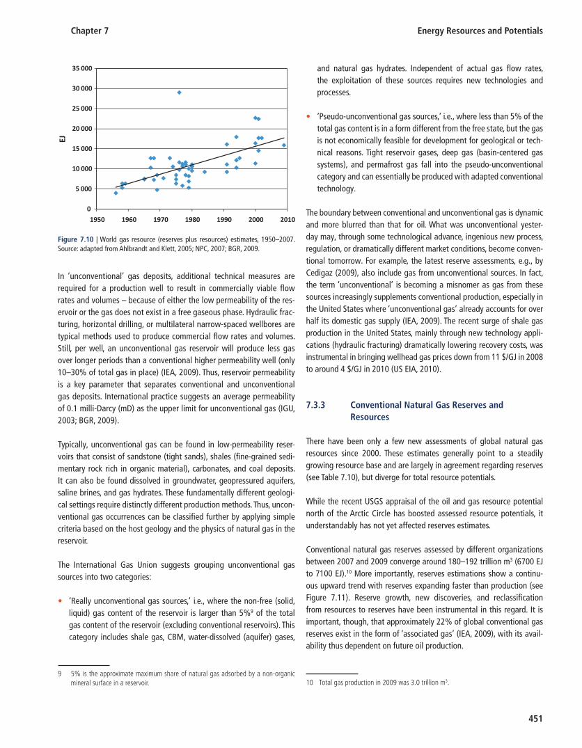
Chapter 7 Energy Resources and Potentials
451
In ‘unconventional’ gas deposits, additional technical measures are required for a production well to result in commercially viable flow rates and volumes – because of either the low permeability of the res-ervoir or the gas does not exist in a free gaseous phase. Hydraulic frac-turing, horizontal drilling, or multilateral narrow-spaced wellbores are typical methods used to produce commercial flow rates and volumes. Still, per well, an unconventional gas reservoir will produce less gas over longer periods than a conventional higher permeability well (only 10–30% of total gas in place) (IEA, 2009 ). Thus, reservoir permeability is a key parameter that separates conventional and unconventional gas deposits. International practice suggests an average permeability of 0.1 milli-Darcy (mD) as the upper limit for unconventional gas (IGU, 2003 ; BGR, 2009 ).
Typically, unconventional gas can be found in low-permeability reser-voirs that consist of sandstone (tight sands), shales (fine-grained sedi-mentary rock rich in organic material), carbonates, and coal deposits. It can also be found dissolved in groundwater, geopressured aquifers, saline brines, and gas hydrates. These fundamentally different geologi-cal settings require distinctly different production methods. Thus, uncon-ventional gas occurrences can be classified further by applying simple criteria based on the host geology and the physics of natural gas in the reservoir.
The International Gas Union suggests grouping unconventional gas sources into two categories:
‘Really unconventional gas sources,’ i.e., where the non-free (solid, •liquid) gas content of the reservoir is larger than 5% 9 of the total gas content of the reservoir (excluding conventional reservoirs). This category includes shale gas, CBM, water-dissolved (aquifer) gases,
and natural gas hydrates. Independent of actual gas flow rates, the exploitation of these sources requires new technologies and processes.
‘Pseudo-unconventional gas sources,’ i.e., where less than 5% of the •total gas content is in a form different from the free state, but the gas is not economically feasible for development for geological or tech-nical reasons. Tight reservoir gases, deep gas (basin-centered gas systems), and permafrost gas fall into the pseudo-unconventional category and can essentially be produced with adapted conventional technology.
The boundary between conventional and unconventional gas is dynamic and more blurred than that for oil. What was unconventional yester-day may, through some technological advance, ingenious new process, regulation, or dramatically different market conditions, become conven-tional tomorrow. For example, the latest reserve assessments, e.g., by Cedigaz ( 2009 ), also include gas from unconventional sources. In fact, the term ‘unconventional’ is becoming a misnomer as gas from these sources increasingly supplements conventional production, especially in the United States where ‘unconventional gas’ already accounts for over half its domestic gas supply (IEA, 2009 ). The recent surge of shale gas production in the United States, mainly through new technology appli-cations (hydraulic fracturing) dramatically lowering recovery costs, was instrumental in bringing wellhead gas prices down from 11 $/GJ in 2008 to around 4 $/GJ in 2010 (US EIA, 2010 ).
7.3.3 Conventional Natural Gas Reserves and Resources
There have been only a few new assessments of global natural gas resources since 2000. These estimates generally point to a steadily growing resource base and are largely in agreement regarding reserves (see Table 7.10 ), but diverge for total resource potentials.
While the recent USGS appraisal of the oil and gas resource potential north of the Arctic Circle has boosted assessed resource potentials, it understandably has not yet affected reserves estimates.
Conventional natural gas reserves assessed by different organizations between 2007 and 2009 converge around 180–192 trillion m 3 (6700 EJ to 7100 EJ). 10 More importantly, reserves estimations show a continu-ous upward trend with reserves expanding faster than production (see Figure 7.11 ). Reserve growth, new discoveries, and reclassification from resources to reserves have been instrumental in this regard. It is important, though, that approximately 22% of global conventional gas reserves exist in the form of ‘associated gas’ (IEA, 2009 ), with its avail-ability thus dependent on future oil production.
0
5 000
10 000
15 000
20 000
25 000
30 000
35 000
1950 1960 1970 1980 1990 2000 2010
EJ
Figure 7.10 | World gas resource (reserves plus resources) estimates, 1950– 2007 . Source: adapted from Ahlbrandt and Klett, 2005 ; NPC, 2007 ; BGR, 2009 .
9 5% is the approximate maximum share of natural gas adsorbed by a non-organic mineral surface in a reservoir. 10 Total gas production in 2009 was 3.0 trillion m 3 .
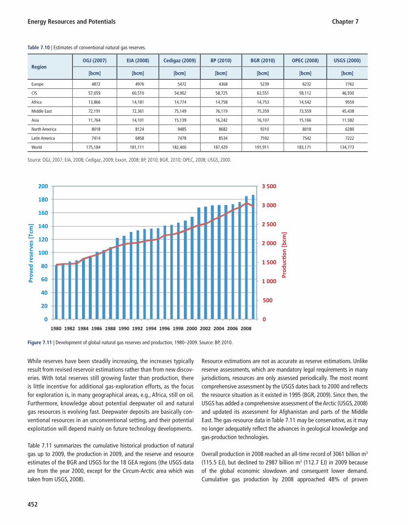
Energy Resources and Potentials Chapter 7
452
While reserves have been steadily increasing, the increases typically result from revised reservoir estimations rather than from new discov-eries. With total reserves still growing faster than production, there is little incentive for additional gas-exploration efforts, as the focus for exploration is, in many geographical areas, e.g., Africa, still on oil. Furthermore, knowledge about potential deepwater oil and natural gas resources is evolving fast. Deepwater deposits are basically con-ventional resources in an unconventional setting, and their potential exploitation will depend mainly on future technology developments.
Table 7.11 summarizes the cumulative historical production of natural gas up to 2009, the production in 2009, and the reserve and resource estimates of the BGR and USGS for the 18 GEA regions (the USGS data are from the year 2000 , except for the Circum-Arctic area which was taken from USGS, 2008 ).
Resource estimations are not as accurate as reserve estimations. Unlike reserve assessments, which are mandatory legal requirements in many jurisdictions, resources are only assessed periodically. The most recent comprehensive assessment by the USGS dates back to 2000 and reflects the resource situation as it existed in 1995 (BGR, 2009 ). Since then, the USGS has added a comprehensive assessment of the Arctic (USGS, 2008 ) and updated its assessment for Afghanistan and parts of the Middle East. The gas-resource data in Table 7.11 may be conservative, as it may no longer adequately reflect the advances in geological knowledge and gas-production technologies.
Overall production in 2008 reached an all-time record of 3061 billion m 3 (115.5 EJ), but declined to 2987 billion m 3 (112.7 EJ) in 2009 because of the global economic slowdown and consequent lower demand. Cumulative gas production by 2008 approached 48% of proven
Table 7.10 | Estimates of conventional natural gas reserves.
Region OGJ ( 2007 ) EIA ( 2008 ) Cedigaz ( 2009 ) BP ( 2010 ) BGR ( 2010 ) OPEC ( 2008 ) USGS ( 2000 )
[bcm] [bcm] [bcm] [bcm] [bcm] [bcm] [bcm]
Europe 4872 4976 5472 4368 5239 6232 7762
CIS 57,059 60,510 54,902 58,725 63,551 58,112 46,930
Africa 13,866 14,181 14,774 14,758 14,753 14,542 9559
Middle East 72,191 72,361 75,149 76,119 75,359 73,559 45,438
Asia 11,764 14,101 15,139 16,242 16,107 15,166 11,582
North America 8018 8124 9485 8682 9310 8018 6280
Latin America 7414 6858 7478 8534 7592 7542 7222
World 175,184 181,111 182,400 187,429 191,911 183,171 134,773
Source: OGJ, 2007 ; EIA, 2008 ; Cedigaz, 2009 ; Exxon, 2008 ; BP, 2010 ; BGR, 2010 ; OPEC, 2008 ; USGS, 2000 .
0
500
1 000
1 500
2 000
2 500
3 000
3 500
0
20
40
60
80
100
120
140
160
180
200
1980 1982 1984 1986 1988 1990 1992 1994 1996 1998 2000 2002 2004 2006 2008
Prod
uc�
on [b
cm]
Prov
ed r
eser
ves
[Tcm
]
Figure 7.11 | Development of global natural gas reserves and production, 1980–2009. Source: BP, 2010 .
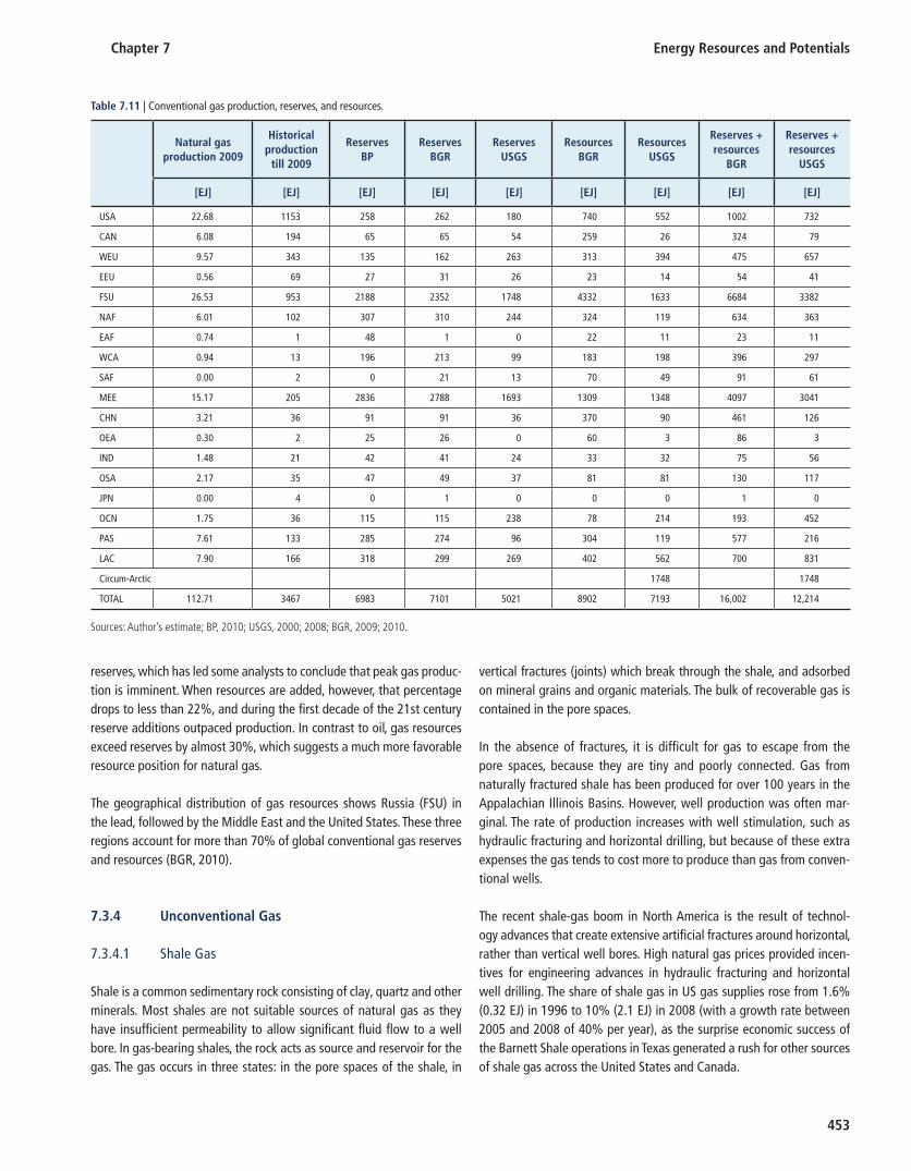
Chapter 7 Energy Resources and Potentials
453
reserves, which has led some analysts to conclude that peak gas produc-tion is imminent. When resources are added, however, that percentage drops to less than 22%, and during the first decade of the 21st century reserve additions outpaced production. In contrast to oil, gas resources exceed reserves by almost 30%, which suggests a much more favorable resource position for natural gas.
The geographical distribution of gas resources shows Russia (FSU) in the lead, followed by the Middle East and the United States. These three regions account for more than 70% of global conventional gas reserves and resources (BGR, 2010 ).
7.3.4 Unconventional Gas
7.3.4.1 Shale Gas
Shale is a common sedimentary rock consisting of clay, quartz and other minerals. Most shales are not suitable sources of natural gas as they have insufficient permeability to allow significant fluid flow to a well bore. In gas-bearing shales, the rock acts as source and reservoir for the gas. The gas occurs in three states: in the pore spaces of the shale, in
vertical fractures (joints) which break through the shale, and adsorbed on mineral grains and organic materials. The bulk of recoverable gas is contained in the pore spaces.
In the absence of fractures, it is difficult for gas to escape from the pore spaces, because they are tiny and poorly connected. Gas from naturally fractured shale has been produced for over 100 years in the Appalachian Illinois Basins. However, well production was often mar-ginal. The rate of production increases with well stimulation, such as hydraulic fracturing and horizontal drilling, but because of these extra expenses the gas tends to cost more to produce than gas from conven-tional wells.
The recent shale-gas boom in North America is the result of technol-ogy advances that create extensive artificial fractures around horizontal, rather than vertical well bores. High natural gas prices provided incen-tives for engineering advances in hydraulic fracturing and horizontal well drilling. The share of shale gas in US gas supplies rose from 1.6% (0.32 EJ) in 1996 to 10% (2.1 EJ) in 2008 (with a growth rate between 2005 and 2008 of 40% per year), as the surprise economic success of the Barnett Shale operations in Texas generated a rush for other sources of shale gas across the United States and Canada.
Table 7.11 | Conventional gas production, reserves, and resources.
Natural gas production 2009
Historical production
till 2009
Reserves BP
Reserves BGR
Reserves USGS
Resources BGR
Resources USGS
Reserves + resources
BGR
Reserves + resources
USGS
[EJ] [EJ] [EJ] [EJ] [EJ] [EJ] [EJ] [EJ] [EJ]
USA 22.68 1153 258 262 180 740 552 1002 732
CAN 6.08 194 65 65 54 259 26 324 79
WEU 9.57 343 135 162 263 313 394 475 657
EEU 0.56 69 27 31 26 23 14 54 41
FSU 26.53 953 2188 2352 1748 4332 1633 6684 3382
NAF 6.01 102 307 310 244 324 119 634 363
EAF 0.74 1 48 1 0 22 11 23 11
WCA 0.94 13 196 213 99 183 198 396 297
SAF 0.00 2 0 21 13 70 49 91 61
MEE 15.17 205 2836 2788 1693 1309 1348 4097 3041
CHN 3.21 36 91 91 36 370 90 461 126
OEA 0.30 2 25 26 0 60 3 86 3
IND 1.48 21 42 41 24 33 32 75 56
OSA 2.17 35 47 49 37 81 81 130 117
JPN 0.00 4 0 1 0 0 0 1 0
OCN 1.75 36 115 115 238 78 214 193 452
PAS 7.61 133 285 274 96 304 119 577 216
LAC 7.90 166 318 299 269 402 562 700 831
Circum-Arctic 1748 1748
TOTAL 112.71 3467 6983 7101 5021 8902 7193 16,002 12,214
Sources: Author’s estimate; BP, 2010 ; USGS, 2000 ; 2008 ; BGR, 2009 ; 2010 .
Energy Resources and Potentials Chapter 7
454
To date, almost all successful shale-gas wells have been in rocks of Paleozoic age, but shales of other ages are being evaluated, particularly Cretaceous shales in Rocky Mountain basins. In other parts of the world shale gas has not yet been produced commercially because of a limited geological knowledge about shale gas and host reservoirs, as well as higher technical and economic costs. However, since 2006 accelerated shale-gas exploration has occurred in both Europe and Asia.
7.3.4.2 Coal-bed Methane
CBM is gas that is adsorbed into the solid matrix of the coal. Its lack of H 2 S content means the gas is considered a ‘sweet gas.’ It is located in various forms in natural fractures (free form), coal pores (free and adsorbed form), and coal structures (absorbed form). The presence of this gas is well known from its occurrence in underground coal mining, where it presents a serious safety risk. CBM is located at depths that range between 300–2000 m and can be extracted by multi-leg, horizontal wells or wells with massive hydraulic fractur-ing. As a result of low pressures and low well-head flow rates, the production of CBM is economically feasible only in the vicinity of gas-demand centers. Thus, its production is feasible in countries with considerable coal basins and where substantial populations exist on the territory of these basins: the United States, Canada, Australia, Russia, Ukraine, China, India, and approximately another 35 coun-tries. CBM is produced commercially in the United States from some 40,000 coal-bed gas wells, and accounts for approximately 9% (1.8 EJ) of total domestic gas production.
The development of CBM in countries outside the United States contin-ues to be slow for several reasons, including unfavorable reservoir char-acteristics, inadequate infrastructure, lack of operating knowledge, and competition from conventional gas. In some cases, leases have changed ownership several times before an operator with the right combination of corporate size, technical know-how, and contractual terms has been able to achieve a successful project.
7.3.4.3 Tight Reservoir (Tight Sands) Gas
Tight sands reservoirs are conventional gas resources located in sedi-mentary basins with less than 0.1 mD permeability, and at a depth of up to 4500 m. These geological structures can be found practi-cally everywhere in the world. Still, countries with large conventional resources in very permeable reservoirs have had a tendency to pay little or no attention to tight reservoirs. Gas production from these reservoirs is developing in countries with mature gas industries (e.g., the United States, Canada, Great Britain, and Russia) and in coun-tries poorly endowed with conventional natural gas resources (e.g., Japan and China). In fact, the distinction between conventional and unconventional tight gas is increasingly blurred, especially in North America. For example, the US EIA no longer lists the production of
tight gas under unconventional gas, and it is now accounted for under conventional gas.
7.3.4.4 Gas in Deep Reservoirs (Basin-centered Gas Systems)
Deep reservoirs are deep sedimentary basins located at depths greater than 4500 m and are usually characterized by high pressures and high temperatures, and the presence of significant acid components (IGU, 1994 ; 2003 ; BGR, 2009 ). Basin-centered gas systems are typically fur-ther characterized by regionally pervasive accumulations that are gas saturated, abnormally pressured, commonly lack a down-dip water con-tact, and have low-permeability reservoirs.
Production from depths larger than 4500 m is technologically challeng-ing. Low porosity and permeability limit gas flow rates to the well bore and require reservoir fracturing and complex horizontal and multilateral production wells. Drilling in tight formations with conventional technol-ogy at depths approaching 4500 m becomes increasingly prohibitive, and the extractable gas per well is lower than that for conventional gas at shallower depths. Deep gas has been explored in North America, North Europe, Russia, and some other regions. Exploration and produc-tion is technically challenging and there are only a few examples of deep-gas production: in the United States (on old exhausted fields and fields close to the consumer), in the North Sea (an old gas-producing region), and in Russia in the super-giant Astrakhan gas field. In all these cases production is constrained by technical, safety, and environmental restrictions.
7.3.4.5 Water-dissolved (Aquifer) Gas
‘Aquifer gas’ refers to CH 4 dissolved and dispersed in groundwater. This can be found practically everywhere as almost all porous rock forma-tions below groundwater tables contain small amounts of CH 4 . As a result of the low solubility of CH 4 in water, the gas content of water at depths less than 1000 m is low (0.3–3 m 3 /m 3 of water) and production is economically unattractive. At greater depths, the CH 4 content can reach 10–15 m 3 /m 3 . In areas under high tectonic stress, gas concentrations of up to 90 m 3 /m 3 can be found (BGR, 2009 ). The gas contained in aquifers exceeds reserves of conventional gas by two orders of magnitude, but even with new extraction technology only a small share of this gas is expected to become commercially viable in the long run.
Unlike conventional and other unconventional gases, the produc-tion of aquifer gas hinges upon the coextraction of the CH 4 substrate water. The process of water lifting and aboveground separation of typi-cally low-concentration CH 4 , as well as subsequent water treatment and disposal/recycling, generally has a low energy payback and thus lacks economic attractiveness. The economics may improve, for exam-ple in regions with high freshwater demand where gas production would be a convenient by-product, or in cases where geopressure and
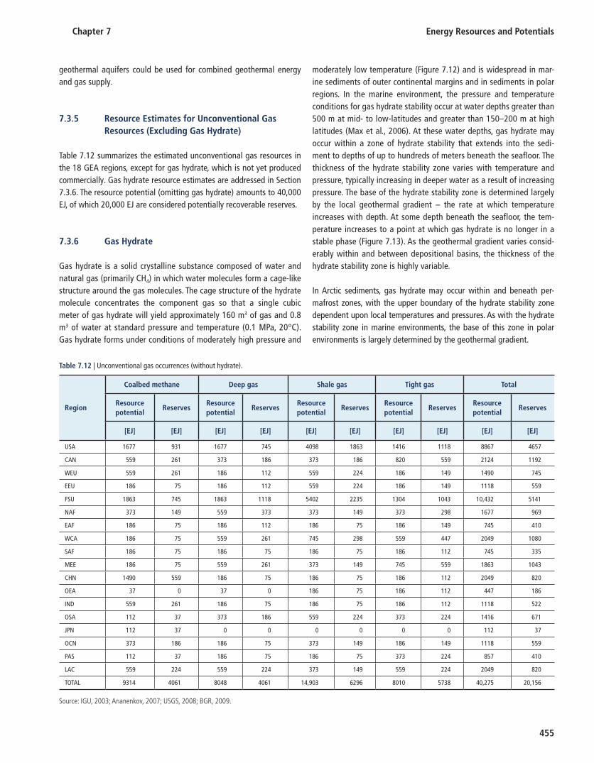
Chapter 7 Energy Resources and Potentials
455
geothermal aquifers could be used for combined geothermal energy and gas supply.
7.3.5 Resource Estimates for Unconventional Gas Resources (Excluding Gas Hydrate)
Table 7.12 summarizes the estimated unconventional gas resources in the 18 GEA regions, except for gas hydrate, which is not yet produced commercially. Gas hydrate resource estimates are addressed in Section 7.3.6 . The resource potential (omitting gas hydrate) amounts to 40,000 EJ, of which 20,000 EJ are considered potentially recoverable reserves.
7.3.6 Gas Hydrate
Gas hydrate is a solid crystalline substance composed of water and natural gas (primarily CH 4 ) in which water molecules form a cage-like structure around the gas molecules. The cage structure of the hydrate molecule concentrates the component gas so that a single cubic meter of gas hydrate will yield approximately 160 m 3 of gas and 0.8 m 3 of water at standard pressure and temperature (0.1 MPa, 20°C). Gas hydrate forms under conditions of moderately high pressure and
moderately low temperature ( Figure 7.12 ) and is widespread in mar-ine sediments of outer continental margins and in sediments in polar regions. In the marine environment, the pressure and temperature conditions for gas hydrate stability occur at water depths greater than 500 m at mid- to low-latitudes and greater than 150–200 m at high latitudes (Max et al., 2006 ). At these water depths, gas hydrate may occur within a zone of hydrate stability that extends into the sedi-ment to depths of up to hundreds of meters beneath the seafloor. The thickness of the hydrate stability zone varies with temperature and pressure, typically increasing in deeper water as a result of increasing pressure. The base of the hydrate stability zone is determined largely by the local geothermal gradient – the rate at which temperature increases with depth. At some depth beneath the seafloor, the tem-perature increases to a point at which gas hydrate is no longer in a stable phase ( Figure 7.13 ). As the geothermal gradient varies consid-erably within and between depositional basins, the thickness of the hydrate stability zone is highly variable.
In Arctic sediments, gas hydrate may occur within and beneath per-mafrost zones, with the upper boundary of the hydrate stability zone dependent upon local temperatures and pressures. As with the hydrate stability zone in marine environments, the base of this zone in polar environments is largely determined by the geothermal gradient.
Table 7.12 | Unconventional gas occurrences (without hydrate).
Region
Coalbed methane Deep gas Shale gas Tight gas Total
Resource potential
ReservesResource potential
ReservesResource potential
ReservesResource potential
ReservesResource potential
Reserves
[EJ] [EJ] [EJ] [EJ] [EJ] [EJ] [EJ] [EJ] [EJ] [EJ]
USA 1677 931 1677 745 4098 1863 1416 1118 8867 4657
CAN 559 261 373 186 373 186 820 559 2124 1192
WEU 559 261 186 112 559 224 186 149 1490 745
EEU 186 75 186 112 559 224 186 149 1118 559
FSU 1863 745 1863 1118 5402 2235 1304 1043 10,432 5141
NAF 373 149 559 373 373 149 373 298 1677 969
EAF 186 75 186 112 186 75 186 149 745 410
WCA 186 75 559 261 745 298 559 447 2049 1080
SAF 186 75 186 75 186 75 186 112 745 335
MEE 186 75 559 261 373 149 745 559 1863 1043
CHN 1490 559 186 75 186 75 186 112 2049 820
OEA 37 0 37 0 186 75 186 112 447 186
IND 559 261 186 75 186 75 186 112 1118 522
OSA 112 37 373 186 559 224 373 224 1416 671
JPN 112 37 0 0 0 0 0 0 112 37
OCN 373 186 186 75 373 149 186 149 1118 559
PAS 112 37 186 75 186 75 373 224 857 410
LAC 559 224 559 224 373 149 559 224 2049 820
TOTAL 9314 4061 8048 4061 14,903 6296 8010 5738 40,275 20,156
Source: IGU, 2003 ; Ananenkov, 2007 ; USGS, 2008 ; BGR, 2009 .
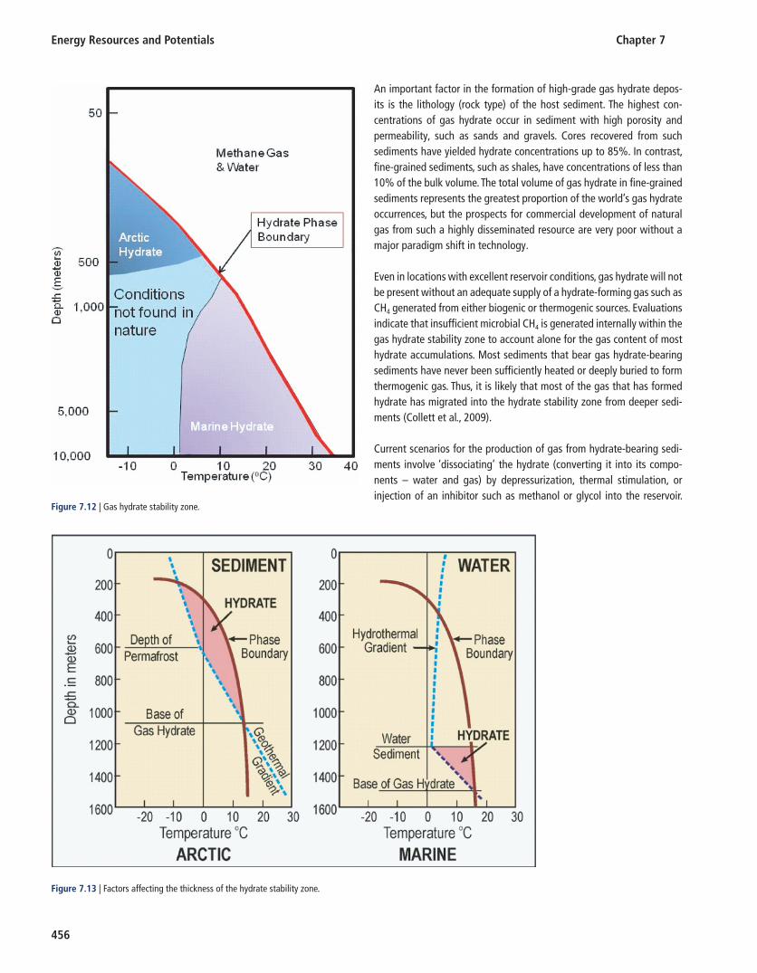
Energy Resources and Potentials Chapter 7
456
An important factor in the formation of high-grade gas hydrate depos-its is the lithology (rock type) of the host sediment. The highest con-centrations of gas hydrate occur in sediment with high porosity and permeability, such as sands and gravels. Cores recovered from such sediments have yielded hydrate concentrations up to 85%. In contrast, fine-grained sediments, such as shales, have concentrations of less than 10% of the bulk volume. The total volume of gas hydrate in fine-grained sediments represents the greatest proportion of the world’s gas hydrate occurrences, but the prospects for commercial development of natural gas from such a highly disseminated resource are very poor without a major paradigm shift in technology.
Even in locations with excellent reservoir conditions, gas hydrate will not be present without an adequate supply of a hydrate-forming gas such as CH 4 generated from either biogenic or thermogenic sources. Evaluations indicate that insufficient microbial CH 4 is generated internally within the gas hydrate stability zone to account alone for the gas content of most hydrate accumulations. Most sediments that bear gas hydrate-bearing sediments have never been sufficiently heated or deeply buried to form thermogenic gas. Thus, it is likely that most of the gas that has formed hydrate has migrated into the hydrate stability zone from deeper sedi-ments (Collett et al., 2009 ).
Current scenarios for the production of gas from hydrate-bearing sedi-ments involve ‘dissociating’ the hydrate (converting it into its compo-nents – water and gas) by depressurization, thermal stimulation, or injection of an inhibitor such as methanol or glycol into the reservoir.
Figure 7.12 | Gas hydrate stability zone.
Figure 7.13 | Factors affecting the thickness of the hydrate stability zone.
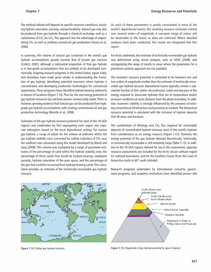
Chapter 7 Energy Resources and Potentials
457
The method utilized will depend on specific reservoir conditions, includ-ing hydrate saturation, porosity, and permeability. Natural gas may also be produced from gas hydrate through a chemical exchange, such as a substitution of CO 2 for CH 4 . This approach has the advantage of seques-tering CO 2 as well as yielding commercial gas production (Graue et al., 2006 ).
In summary, the volume of natural gas contained in the world’s gas hydrate accumulations greatly exceeds that of known gas reserves (Collett, 2002 ), although a substantial proportion of that gas hydrate is in low-grade accumulations that are unlikely to be developed com-mercially. Ongoing research programs in the United States, Japan, India, and elsewhere have made great strides in understanding the forma-tion of gas hydrate, identifying potential reservoirs where hydrate is concentrated, and developing production technologies for commercial exploitation. These programs have identified hydrate-bearing sediments in dozens of locations ( Figure 7.14 ). Thus far, the vast energy potential of gas hydrate resources has not been proven commercially viable. There is, however, growing evidence that natural gas can be produced from high-grade gas hydrate accumulations with existing conventional oil and gas production technology (Moridis et al., 2008 ).
Estimates of the gas hydrate resource potential for each of the 18 GEA regions was undertaken by first segregating each region into sepa-rate subregions based on the local depositional setting. For marine gas hydrate, a range of values for the volume of sediment within the gas hydrate stability zone (corrected for sulfate reduction of CH 4 near the seafloor) was calculated using the model developed by Wood and Jung ( 2008 ). This volume was multiplied by a range of parameter esti-mates of the percentage of sand within the hydrate stability zone, the percentage of those sands that would be hydrate-bearing, sandstone porosity, hydrate saturation of the pore space, and the percentage of the gas that could be recovered from hydrate-bearing sands. This calcu-lation provides an estimate of the technically recoverable gas hydrate resource.
As each of these parameters is poorly constrained in most of the world’s depositional basins, the resulting resource estimates extend over several orders of magnitude. A narrower range of values will be obtainable in the future as data are collected. Where detailed analyses have been conducted, the results are integrated into this report.
For Arctic sediments, the estimate of technically recoverable gas hydrate was determined using recent analyses, such as USGS ( 2008 ), and extrapolating the range of results to areas where the parameters for a petroleum-systems approach are not available.
The economic resource potential is estimated to be between one and two orders of magnitude smaller than the estimate of technically recov-erable gas hydrate because depositional basins typically contain a sub-stantial fraction of thin and/or discontinuous sands and because of the energy required to dissociate hydrates that are at temperature and/or pressure conditions at some distance from the phase boundary. In addi-tion, economic viability is strongly influenced by the presence of exist-ing conventional infrastructure and proximity to markets. The theoretical resource potential is calculated with the inclusion of hydrate deposits that fill veins and fractures.
The combination of lithology and CH 4 flux required for extractable deposits of concentrated hydrate removes most of the world’s hydrate from consideration as an energy resource ( Figure 7.15 ). However, the energy potential of the gas hydrate deemed theoretically, technically, or economically recoverable is still extremely large ( Table 7.13 ). In addi-tion to the 18 GEA regions defined for use in this assessment, separate resource assessments are included for the Arctic Ocean without regard for national boundaries, and for the Southern Ocean (from the coast of Antarctica north to 60° south latitude).
Research programs undertaken by international consortia, govern-ment programs, and academic institutions have identified proven and
Figure 7.14 | Global gas hydrate locations. Figure 7.15 | Magnitude of gas hydrate potential by type of deposit.

Energy Resources and Potentials Chapter 7
458
probable gas hydrate locations along continental margins and in polar regions throughout the world, although characterization of deposits is limited to relatively few locations.
7.3.6.1 Overall Unconventional Gas Resources (Including Gas Hydrate)
Table 7.14 summarizes the current understanding of global uncon-ventional gas resources. Gas hydrate and water-dissolved gas are the most abundant, and are also relatively evenly distributed geographi-cally. CBM, shale gas, and deep formation gas appear to be less evenly distributed, but this may well be the consequence of limited geological knowledge through historically low interest. Gas is likely to be found in the tighter formations of all sedimentary basins of the world, but actual quantities can only be confirmed and delineated through dedicated and costly exploration activities.
7.3.7 Abiogenic Gas Theory
While petroleum (oil and gas) occurrences are commonly thought of as being derived from biological substances, i.e., by the thermal decompo-sition of organic matter or by microbial processes (Lollar et al., 2002 ), since the very beginning of the ‘petroleum age’ there has been a sub-stantial amount of skepticism voiced about its exclusively biological origin (e.g., Mendeleev, 1877 ; Kudryavtsev, 1951 ; Gold and Soter, 1980 ; 1982 ; Gold, 1999 ; Kenney et al., 2009 ). According to the proponents of an abiogenic origin of hydrocarbons, CH 4 and oil are also, perhaps even predominantly, formed well below the usual depths of oil and gas deposits.
By comparing the carbon and hydrogen stable isotope signatures of CH 4 seeping from hard rock mines of Canadian and Fennoscandian shields, with microbial and thermogenic CH 4 , Lollar et al. ( 2002 ) confirmed the abiogenic formation of hydrocarbons within the Earth’s crust. Abiogenic hydrocarbon formation is attributed to the reduction of CO 2 in hydro-thermal water-rock interactions similar to Fischer-Tropsch reactions and serpentinization of ultramafic rock. However, the lack of abiogenic isotope signatures in current conventional gases means these authors doubt that abiogenic formation is a significant hydrocarbon source. In contrast, the ‘modern Russian-Ukrainian’ theory of the origins of hydro-carbons postulates that petroleum is a primordial material of deep origin which is transported at high pressures via ‘cold’ eruptive proc-esses into the crust of the Earth (Kenney et al., 2002 ). Much of this theory has developed through chemistry and chemical thermodynamics. One conclusion from the theory is that the origin of hydrocarbon mol-ecules (except CH 4 ) from biogenic ones in the temperature and pressure regimes of the Earth’s near-surface crust is in violation of the second law of thermodynamics (Kenney, 1996 ).
The abiogenic theory has been applied extensively across the former Soviet Union and has revealed 80 oil and gas fields in the Caspian dis-trict with production from the crystalline basement rock. Other examples
Table 7.13 | Recoverable gas hydrate resource potentials.
Region
Theoretical potential
Technical potentialEconomic potential
[EJ] [EJ] [EJ]
USA 782–122,128 395–12,213 0–1229
CAN 298–71,049 142–71,049 0–712
WEU 37–490,153 11–11,758 0–1177
EEU 0–820 0–83 0
FSU 820–80,997 402–8100 0–808
NAF 0–30,439 0–1449 0–71
EAF 0–155,883 4–15,588 0–779
WCA 37–211,061 22–21,106 0–1054
SAF 75–208,676 34–20,868 0–1043
MEE 0–30,439 7–3044 0–30
CHN 0–14,158 4–1416 0–142
OEA 0–21,386 4–2139 0–212
IND 37–49,589 11–4959 0–496
OSA 0–27,682 7–2768 0–276
JPN 37–3726 19–373 0–37
OCN 37–53,427 11–5343 0–533
PAS 37–205,323 15–20,532 0–2053
LAC 149–198,766 67–19,877 0–1986
SOO* 75–357,779 37–35,782 0
ARC** 75–439,409 45–43,926 0
Total 2,496–2,772,889 1237–238,428 0–12,638
* Southern Ocean
** Arctic Ocean
Table 7.14 | Global unconventional gas resources.
Really unconventional
Water-dissolved (aquifer) gas (depth up to 4.5 km)
8000–10,000 Tm 3 300,000–370,000 EJ
Gas of hydrates (including permafrost metastable hydrates)
2500–21,000 Tm 3 90,000–780,000 EJ
Shale gas 380–420 Tm 3 14,000–15,500 EJ
CBM (up to depth 4.5 km) 200–250 Tm 3 7500–9300 EJ
Pseudounconventional
Dense reservoirs (tight sands) gas (depth up to 4.5 km)
180–220 Tm 3 6700–8200 EJ
Deep reservoirs (depth 4.5–7.0 km) gas 200–300 Tm 3 7500–11,200 EJ
Source: Ananenkov, 2007 .

Chapter 7 Energy Resources and Potentials
459
have been found in the western Siberian cratonic-rift sedimentary basin with numerous fields producing from the crystalline basement; on the northern flanks of the Dneiper-Donotz basin; and elsewhere in Azerbaijan, Tatarstan, and Asian Siberia.
The theory also postulates that many of the world’s oil and gas fields are being continuously recharged from deeper horizons with abiogenic hydrocarbons, so making the fields ‘effectively inexhaustible,’ and there-fore oil and gas fields now considered exhausted should be thoroughly investigated to ascertain the quantities of oil and gas that may have accumulated since the fields were shut-in. In view of the above consid-erations, Kenney et al. ( 2009 ) believe that petroleum abundances are limited by little more than the quantities of its constituent elements that were incorporated into the Earth at the time of its formation and the petroleum industry is only now “entering its adolescence.”
Gold ( 1988 ) argues that hydrocarbons are of primordial origin without biological derivation. The presence of hydrocarbons in the planetary system, e.g., the atmospheres of Jupiter, Saturn, or Neptune contain enormous amounts of CH 4 and other hydrocarbons, while Titan, a satel-lite of Saturn, has a CH 4 and ethane atmosphere that is unlikely the result of biological processes. Rather, carbonaceous chondrite meteor-ites are thought to have brought carbon to the Earth during its forma-tion. Subjected to the appropriate heat and pressure domains present at great depths, e.g., in the vicinity of magma cooling, the carbonaceous material would produce hydrocarbons, chiefly CH 4 , as well as hydrogen and CO 2 , which is subsequently outgassed to the upper layers of the Earth’s crust. Such an environment is also quite amenable for the forma-tion of heavier hydrocarbon molecules.
The discovery of microbial life in ocean vents too deep for photosynthesis is used by Gold ( 1999 ) in support of the abiogenic gas theory. Instead of pho-tosynthesis, the large amounts of CH 4 in these hydrothermal vents migrat-ing from deeper levels supply the energy required for life in chemical form. In addition, the existence of anaerobic bacteria in rock structures and CH 4 environments at depths of more than 4 km is another indication of abio-genic CH 4 . In turn, bacteria brought along the upward-migrating hydrocar-bons explain the existence of certain biomarkers in extracted petroleum commonly associated with the decomposition of organic matter.
The abiogenic origin of hydrocarbon debate dates back to the mid-19th century and since then the theory has undergone extensive development, refinement, and application. More than 4000 articles on the theory have been published (Odell, 2010 ) and numerous scientific conferences have been held to debate and evaluate the theory. The existence of abiogenic formation of CH 4 and hydrocarbon gases within the Earth has been con-firmed (Lollar et al., 2002 ), but their substantial or exclusive contribution to, and replenishment of, current gas and oil deposits making hydrocar-bons a quasi renewable source as proposed by the Russian-Ukrainian theory remains a matter of controversy.
7.3.8 Natural Gas Supply Cost Curves
The aggregate global gas supply cost curve shown in Figure 7.16 plots the potential long-term contributions from conventional and unconven-tional gas reserves and resources (see Tables 7.11 and 7.12 ) against their estimated production costs. The costs do not include taxes or royal-ties, nor do they include external environmental or social costs associ-ated with gas production.
Conventional gas reserves and resources amount to about 12,000 EJ (~300 trillion m 3 ). In this analysis, the costs of producing conven-tional resources range from 0.50–3.50 $/GJ. The supply curve sug-gests some 5000 EJ of conventional gas can be produced for around 1 $/GJ or less at 2007 prices and exchange rates (these supply costs are not the actual prices in the market place). To put this amount of gas into perspective, the cumulative past gas production amounts to 3467 EJ.
Unconventional gas reservoirs are very diverse in their geological struc-ture, location, and accessibility and each deposit requires a specifically tailored extraction technology. Production cost estimates vary consider-ably, from less than 2 $/GJ for shale gas from very permeable reservoirs, CBM, or onshore gas hydrate to more than 13 $/GJ for offshore deep gas reservoirs. The supply cost curve of Figure 7.16 includes 28,000 EJ of unconventional gas (reserves plus 20% of resources assumed to become resources before 2050) and 5000 EJ of hydrate gas. The production costs of 40% of unconventional reserves are estimated at 2–5 $/GJ, while the remaining 60% of reserves plus 20% of the resources can eventually be recovered for 5–13 $/GJ.
Almost all unconventional resources are characterized by low per-meability, and their extraction requires intensive reservoir stimula-tion through various techniques, e.g., horizontal drilling, multi-leg
0123456789
1011121314
0 5000 10000 15000 20000 25000 30000 35000 40000 45000
Prod
uc�
on c
osts
, $/G
J
EJ
Current Technology
2050 Technology
Figure 7.16 | Aggregate world-supply cost curve 11 for conventional and unconven-tional natural gas. Source: Rogner, 1997 ; Rogner et al., 2000 ; USGS, 2000 ; 2008 ; Aguilera et al., 2009 ; BGR, 2009 .
11 See footnote 7.
Energy Resources and Potentials Chapter 7
460
completion, hydraulic fracturing, reservoir acid treatment (for carbon-ates), and thermal stimulation (for hydrate).
Regarding actual production experience with unconventional gas, the US gas industry is very much in the lead globally. Faced with perpetu-ally declining production from conventional gas reserves, the indus-try sought alternatives. National fiscal policy created incentives for technological advances in exploration and production of unconven-tional gas. This led to a ‘quiet revolution’ in North America, where techniques, such as horizontal drilling and hydraulic fracturing, are allowing access to deposits of unconventional tight and shale gas, and of CBM at much lower costs than thought possible five years ago. In some cases, costs are now lower than those in conventional gas projects.
Costs for the production of gas from hydrate have yet to be deline-ated and to date no commercial production experience exists. Costs will depend on a variety of factors ranging from geological conditions (e.g., permeability of sediments, reservoir pressure, location, and size of hydrate deposits) to the necessary selective adaptation of explora-tion and extraction technology. For example, free gas trapped by a hydrate deposit may well be producible with conventional produc-tion technology for natural gas. Generally, site development will be more complex, and hence costlier, than that for conventional natu-ral gas. The estimates of economically recoverable gas quantities from hydrate are based inherently on the expected competition with conventional and other unconventional gas occurrences and their respective future costs, and a range of 8–12 $/GJ for gas from hydrate appears plausible.
7.3.9 Environmental and Social Implications
In addition to concerns similar to those relating to oil development, natural gas development raises several other issues.
CH 4 , the chief constituent of natural gas, has a very high global warming potential and special care is needed to minimize leaks to the atmos-phere. Leakage of gas behind casings of abandoned and ‘sealed’ oil and gas wells leads to gas entering shallow aquifers, thus degrading potable water resources. This is a significant environmental issue, identified by the US Environmental Protection Agency (US EPA) as a major concern. It can be addressed through better well-abandonment regulations, as well as enforcement of collection or flaring of small and low-grade CH 4 emissions.
Shale-gas development involving deep hydraulic fracturing in the United States has caused serious concerns about drinking water contamination and land degradation (Arthur et al. 2008 ). The US EPA has undertaken a scientific study to investigate the potential risks to drinking water from hydraulic fracturing and will consider the need for additional health and safety regulations.
Exploitation of sour gas resources requires special attention to escape of H 2 S during production and SO x during processing. Long-term stock-age of elemental sulfur from gas plants is of environmental concern in areas such as Kazakhstan and western Canada because of distance-to-sea transportation (costs) and the oncoming world sulfur surplus as more sulfurous feedstocks are processed. For example, Tengizchevroil in Kazakhstan has been fined repeatedly for failure to meet contractual obligations in sulfur management. However, the environmental impact of elemental sulfur is small because it is inert.
Production of gas from hydrate involves potential adverse environmen-tal consequences comparable to those of conventional natural gas. Appropriate environmental management and safety measures exist to minimize potential harmful effects. However, two threats are hydrate specific. First, destabilization of the seabed may cause subsidence and land slippage, including blow outs. Second, gas hydrate utilization may adversely affect the habitat of microorganisms and other forms of bio-coenosis systems whose metabolisms depend on CH 4 from hydrate and which form an essential part of the food chain for mussels and beard worms (BGR, 2009 ). Both threats are generally considered of a local nature and manageable.
7.3.10 Summary
The global occurrence of natural gas is enormous and a significant por-tion of the total volume occurs in technically exploitable reservoirs. With regard to unconventional gas resources, the recent boom of shale-gas production in the United States is one example of how quickly technical change stimulated by declining conventional reserves and high market prices can reverse the overall supply outlook and price expectations.
The term ‘unconventional’ is becoming a misnomer, especially with respect to tight gas, shale gas, and CBM. Still, enormous technical chal-lenges exist in the development of innovative exploration and produc-tion technology.
Broad-ranging technology impacts can take decades from initial con-cept to large-scale implementation. In addition, the energy needed to produce unconventional gas is usually higher than that for conventional gas. In the case of gas hydrate, this can reduce the net energy gain by up to 20% or more. Gas hydrate represents the largest of the unconven-tional natural gas resource options. Yet it is currently unclear how much gas hydrate can be exploited, both technically and economically. Field testing of marine and Arctic reservoirs is planned for the near term, and the results of these tests will determine their commercial viability. The development of gas hydrate has important implications, as it is wide-spread along the margins of every continent and, as such, includes areas that lack conventional oil and gas resources.
It is important, however, that progress in exploiting unconventional gases will depend on environmental regulation and suitable management

Chapter 7 Energy Resources and Potentials
461
practices, since many of these resources are in remote and ecologically sensitive areas.
7.4 Coal
7.4.1 Overview
Coal is a combustible, sedimentary, organic rock composed mainly of carbon, hydrogen, and oxygen. It is a fossil fuel formed from vegeta-tion lying between rock strata and altered by the combined effects of pressure and heat over millions of years. Coal deposits can be found in sedimentary basins of various geological ages. Dependent on age, depo-sitional conditions, and geological history, the nature of coal deposits and the quality and characteristics of coal vary in terms of heat value, reaction characteristics, and impurities.
The degree of change undergone by coal as it matures from peat to anthracite – known as coalification – defines its physical and chemical properties and is referred to as the ‘rank’ of the coal. Low-rank coals, such as lignite and sub-bituminous coals, are characterized by high moisture levels, low carbon content, and a consequently low energy content. These coals are typically used locally, predominantly power generation. Higher rank hard coals, i.e., anthracite and bituminous coals, have a higher car-bon content and lower moisture content, which result in higher energy quantities per unit mass of coal. Hard coals are produced both for domes-tic and export markets, including power generation, iron and steel mak-ing processes, and chemical industries (WCI, 2008 ; IEA, 2008a ). The large variety of different coal characteristics and specific energy values mean that assessments of reserve and resource are rather challenging.
Efforts to estimate global coal reserves and resources can be traced back to the beginning of the 20th century ( Table 7.15 ). While there has
been a steady increase in resource estimates, there has been consider-able fluctuation in the estimates of proven hard-coal reserves.
7.4.2 Coal Production
Global hard-coal production amounted to 2.24 Gt in 1950 and has tri-pled since then, with 6.94 Gt produced in 2009. Three distinct periods occurred. A steady annual increase of about 64 Mt between 1950–1986, a period of stagnation from 1988–2000, and a dramatic increase of 260 Mt/yr or 4.7% from 2000–2009 (BP, 2010 ). The first period was char-acterized by a slight growth of coal consumption in the Organisation of Economic Co-Operation and Development (OECD) countries, a static situation in the FSU and marked increases in China, the rest of Asia, and Africa. The period of stagnation coincides with the collapse of cen-trally controlled economies. The unprecedented 50% increase in coal production since 2000 is primarily because of the economic upsurge of China and East Asia (see Table 7.16 ). Since 1981, coal production in the European Union (EU) has decreased by more than half and by one-third in the countries of the FSU; it has remained virtually constant in the OECD countries.
The reason for the marked increase in coal production lies in the relative abundance and broad geographical distribution of coal reserves and the comparatively low cost of coal production from shallow coal deposits. Coal is a domestically available energy source in many countries, and offers relative energy independence and foreign exchange savings.
Table 7.16 details the 2008 coal production for the 18 GEA regions. A heat value of 16.5 MJ/kg demarcates hard coal (bituminous and high-energy sub-bituminous coals) and soft brown coal (lignite and low-energy sub-bituminous coals). In 2008 world coal production amounted to 6799 Mt: 5774 Mt of hard coal and 1025 Mt of lignite/brown coal. Table 7.16 shows that:
China and the United States together account for 56% of world coal •production.
Latin and South America and Africa together produce less than 6% •of world coal.
Asia has developed into the major coal-producing region in the •world.
7.4.3 Reserves
Universally applicable, geological, quality, and technological criteria have yet to be uniformly applied, so assessments of global coal reserves and resources are subject to uncertainty. Most importantly, without a clear distinction between the quality or rank of coals and their spe-cific energy contents, which can vary between 5–30 MJ/kg, aggregate
Table 7.15 | Historical development of hard coal resource estimates.
Source Reserves (Gt) Resources (Gt)
International Geological Congress (IGC) 1913
312 4399
World Power Conference (WPC) 1936 623 5269
World Energy Conference (WEC) 1974 998 7065
Federal Institute of Geo-Sciences and Mineral Resources (BGR) 2007
736 8818
Federal Institute of Geo-Sciences and Mineral Resources (BGR) 2010
723 17,167 a
World Energy Council (WEC) 2010 861 – b
a BGR has included in the 2010 global hard coal resources fi gures, hypothetical coal resources in Canada and the United States, which have almost doubled the hard-coal resources fi gures published in 2007 .
b The World Energy Council does not publish global coal resources fi gures.
Source: adapted from Fettweis, 1976 .
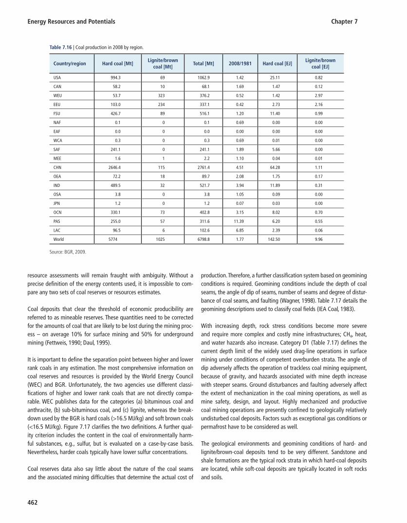
Energy Resources and Potentials Chapter 7
462
resource assessments will remain fraught with ambiguity. Without a precise definition of the energy contents used, it is impossible to com-pare any two sets of coal reserves or resources estimates.
Coal deposits that clear the threshold of economic producibility are referred to as mineable reserves. These quantities need to be corrected for the amounts of coal that are likely to be lost during the mining proc-ess – on average 10% for surface mining and 50% for underground mining (Fettweis, 1990 ; Daul, 1995 ).
It is important to define the separation point between higher and lower rank coals in any estimation. The most comprehensive information on coal reserves and resources is provided by the World Energy Council (WEC) and BGR. Unfortunately, the two agencies use different classi-fications of higher and lower rank coals that are not directly compa-rable. WEC publishes data for the categories (a) bituminous coal and anthracite, (b) sub-bituminous coal, and (c) lignite, whereas the break-down used by the BGR is hard coals (>16.5 MJ/kg) and soft brown coals (<16.5 MJ/kg). Figure 7.17 clarifies the two definitions. A further qual-ity criterion includes the content in the coal of environmentally harm-ful substances, e.g., sulfur, but is evaluated on a case-by-case basis. Nevertheless, harder coals typically have lower sulfur concentrations.
Coal reserves data also say little about the nature of the coal seams and the associated mining difficulties that determine the actual cost of
production. Therefore, a further classification system based on geomining conditions is required. Geomining conditions include the depth of coal seams, the angle of dip of seams, number of seams and degree of distur-bance of coal seams, and faulting (Wagner, 1998 ). Table 7.17 details the geomining descriptions used to classify coal fields (IEA Coal, 1983 ).
With increasing depth, rock stress conditions become more severe and require more complex and costly mine infrastructures; CH 4 , heat, and water hazards also increase. Category D1 ( Table 7.17 ) defines the current depth limit of the widely used drag-line operations in surface mining under conditions of competent overburden strata. The angle of dip adversely affects the operation of trackless coal mining equipment, because of gravity, and hazards associated with mine depth increase with steeper seams. Ground disturbances and faulting adversely affect the extent of mechanization in the coal mining operations, as well as mine safety, design, and layout. Highly mechanized and productive coal mining operations are presently confined to geologically relatively undisturbed coal deposits. Factors such as exceptional gas conditions or permafrost have to be considered as well.
The geological environments and geomining conditions of hard- and lignite/brown-coal deposits tend to be very different. Sandstone and shale formations are the typical rock strata in which hard-coal deposits are located, while soft-coal deposits are typically located in soft rocks and soils.
Table 7.16 | Coal production in 2008 by region.
Country/region Hard coal [Mt] Lignite/brown
coal [Mt] Total [Mt] 2008/1981 Hard coal [EJ]
Lignite/brown coal [EJ]
USA 994.3 69 1062.9 1.42 25.11 0.82
CAN 58.2 10 68.1 1.69 1.47 0.12
WEU 53.7 323 376.2 0.52 1.42 2.97
EEU 103.0 234 337.1 0.42 2.73 2.16
FSU 426.7 89 516.1 1.20 11.40 0.99
NAF 0.1 0 0.1 0.69 0.00 0.00
EAF 0.0 0 0.0 0.00 0.00 0.00
WCA 0.3 0 0.3 0.69 0.01 0.00
SAF 241.1 0 241.1 1.89 5.66 0.00
MEE 1.6 1 2.2 1.10 0.04 0.01
CHN 2646.4 115 2761.4 4.51 64.28 1.11
OEA 72.2 18 89.7 2.08 1.75 0.17
IND 489.5 32 521.7 3.94 11.89 0.31
OSA 3.8 0 3.8 1.05 0.09 0.00
JPN 1.2 0 1.2 0.07 0.03 0.00
OCN 330.1 73 402.8 3.15 8.02 0.70
PAS 255.0 57 311.6 11.39 6.20 0.55
LAC 96.5 6 102.6 6.85 2.39 0.06
World 5774 1025 6798.8 1.77 142.50 9.96
Source: BGR, 2009 .
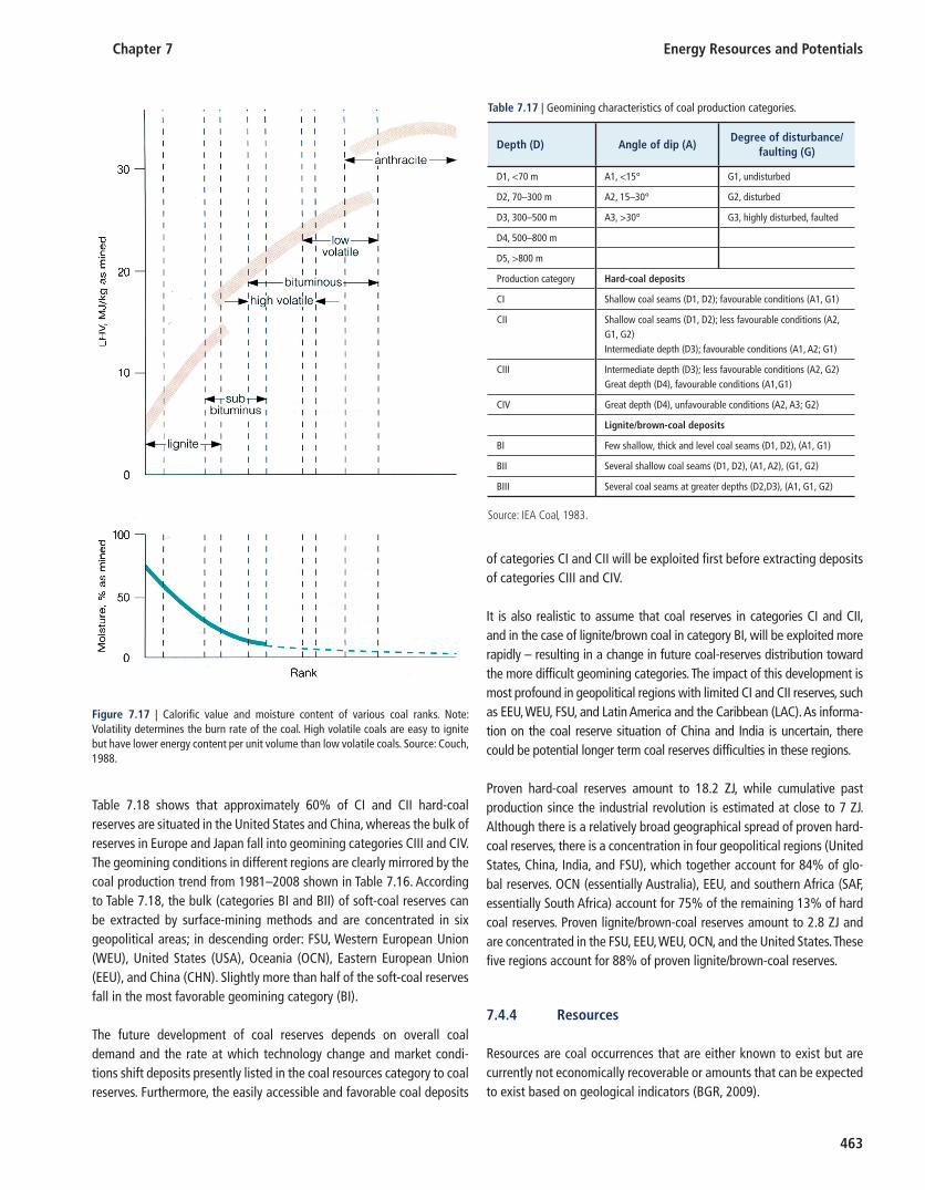
Chapter 7 Energy Resources and Potentials
463
Table 7.18 shows that approximately 60% of CI and CII hard-coal reserves are situated in the United States and China, whereas the bulk of reserves in Europe and Japan fall into geomining categories CIII and CIV. The geomining conditions in different regions are clearly mirrored by the coal production trend from 1981–2008 shown in Table 7.16 . According to Table 7.18 , the bulk (categories BI and BII) of soft-coal reserves can be extracted by surface-mining methods and are concentrated in six geopolitical areas; in descending order: FSU, Western European Union (WEU), United States (USA), Oceania (OCN), Eastern European Union (EEU), and China (CHN). Slightly more than half of the soft-coal reserves fall in the most favorable geomining category (BI).
The future development of coal reserves depends on overall coal demand and the rate at which technology change and market condi-tions shift deposits presently listed in the coal resources category to coal reserves. Furthermore, the easily accessible and favorable coal deposits
of categories CI and CII will be exploited first before extracting deposits of categories CIII and CIV.
It is also realistic to assume that coal reserves in categories CI and CII, and in the case of lignite/brown coal in category BI, will be exploited more rapidly – resulting in a change in future coal-reserves distribution toward the more difficult geomining categories. The impact of this development is most profound in geopolitical regions with limited CI and CII reserves, such as EEU, WEU, FSU, and Latin America and the Caribbean (LAC). As informa-tion on the coal reserve situation of China and India is uncertain, there could be potential longer term coal reserves difficulties in these regions.
Proven hard-coal reserves amount to 18.2 ZJ, while cumulative past production since the industrial revolution is estimated at close to 7 ZJ. Although there is a relatively broad geographical spread of proven hard-coal reserves, there is a concentration in four geopolitical regions (United States, China, India, and FSU), which together account for 84% of glo-bal reserves. OCN (essentially Australia), EEU, and southern Africa (SAF, essentially South Africa) account for 75% of the remaining 13% of hard coal reserves. Proven lignite/brown-coal reserves amount to 2.8 ZJ and are concentrated in the FSU, EEU, WEU, OCN, and the United States. These five regions account for 88% of proven lignite/brown-coal reserves.
7.4.4 Resources
Resources are coal occurrences that are either known to exist but are currently not economically recoverable or amounts that can be expected to exist based on geological indicators (BGR, 2009 ).
Figure 7.17 | Calorifi c value and moisture content of various coal ranks. Note: Volatility determines the burn rate of the coal. High volatile coals are easy to ignite but have lower energy content per unit volume than low volatile coals. Source: Couch, 1988 .
Table 7.17 | Geomining characteristics of coal production categories.
Depth (D) Angle of dip (A)Degree of disturbance/
faulting (G)
D1, <70 m A1, <15° G1, undisturbed
D2, 70–300 m A2, 15–30° G2, disturbed
D3, 300–500 m A3, >30° G3, highly disturbed, faulted
D4, 500–800 m
D5, >800 m
Production category Hard-coal deposits
CI Shallow coal seams (D1, D2); favourable conditions (A1, G1)
CII Shallow coal seams (D1, D2); less favourable conditions (A2, G1, G2) Intermediate depth (D3); favourable conditions (A1, A2; G1)
CIII Intermediate depth (D3); less favourable conditions (A2, G2) Great depth (D4), favourable conditions (A1,G1)
CIV Great depth (D4), unfavourable conditions (A2, A3; G2)
Lignite/brown-coal deposits
BI Few shallow, thick and level coal seams (D1, D2), (A1, G1)
BII Several shallow coal seams (D1, D2), (A1, A2), (G1, G2)
BIII Several coal seams at greater depths (D2,D3), (A1, G1, G2)
Source: IEA Coal, 1983 .

Energy Resources and Potentials Chapter 7
464
Resources are shown as in situ amounts; the eventually extractable quantities will be significantly lower. As a result of the large reserve base and the considerable costs associated with the exploration and delin-eation of resources that may potentially be at the cross-over threshold to reserves, there is limited economic incentive to expand the reserve base beyond a certain range, commonly expressed in terms of years of reserves at current production levels. In the case of coal this is more than 100 years (Wellmer, 2008 ).
The global in situ coal resource data in EJ of Table 7.19 were derived from regional estimates of physical in situ quantities by applying the heating values of coal reserves of these regions areas published by the BGR (Rempel et al., 2007 ).
While coal resources are 20 times higher than known extractable coal reserves, there is uncertainty about the minable portion of these in situ quantities. Information on the geomining conditions of coal resources is insufficient for a reliable production assessment. For example, most of the better delineated coal resources are situated at greater depths and thus belong to geomining categories CIII and CIV. Extraction ratios in geologically difficult coal deposits can be below 40% (Kundel, 1985 ; Daul, 1995 ; USGS, 2009 ). Since many of the ‘in situ’ hard-coal resource deposits are in narrow seams at depths of more than 1000 m, an overall
recovery rate of 20% may well be achievable practically. For example, 60% of coal resources in China are found at depths deeper than of 1000 m (Pan, 2005 ; Minchener, 2007 ). Without new extraction methods, a 20% recovery rate puts the portion of coal resources that eventually could become available as reserves to 87,154 EJ.
7.4.5 Coal Mining Technology
The past 50 years have witnessed remarkable improvements in coal mining technology and productivity. Mechanization and the adoption of engineering-systems approaches resulted in a fourfold increase in labor productivity between 1980 and 2000. In surface mining, bucket-wheel excavators are employed under soft overburden conditions, while drag lines are used under hard overburden conditions, where the overburden strata has to be blasted to expose the coal. In underground mining, manual labor is becoming extinct, except in marginal micromines in developing countries. Coal is now mined by powerful continuous-min-ing machines in room and pillar mining, and pillar recovery operations. As a result of mechanization, safety in underground coal mining has improved and productivities have increased substantially. Output from individual longwall faces has increased more than 10 times over the past 30 years.
Table 7.18 | Hard-coal and lignite/brown-coal reserves in terms of surface and mining potential and geomining conditions.
Region
Hard coal Lignite/brown coal
Total reserves
[EJ]
Surface [EJ]
Underground [EJ]
Category [EJ] Total reserves
[EJ]
Surface [EJ]
Categrory [EJ]
C I C II C III C IV B I B II B III
USA 5856 2342 3514 3924 1347 586 0 371 371 186 186 0
CAN 110 82 27 64 29 18 0 27 27 21 5 0
WEU 67 0 67 0 11 34 22 421 379 253 126 42
EEU 457 32 425 32 32 197 197 198 159 99 60 40
FSU 3306 694 2612 298 926 1455 628 1037 933 622 311 104
NAF 2 1 1 0 1 1 0 0 0 0 0 0
EAF 0 0 0 0 0 0 0 0 0 0 0 0
WCA 9 4 4 2 2 2 2 0 0 0 0 0
SAF 757 144 613 287 212 204 53 0 0 0 0 0
MEE 10 2 8 0 3 4 3 0 0 0 0 0
CHN 4387 965 3422 1579 1623 965 219 106 64 32 32 43
OEA 119 45 74 38 19 34 27 20 20 10 10 0
IND 1856 612 1243 612 1021 223 0 42 42 29 13 0
OSA 11 7 4 9 2 0 0 28 28 14 14 0
JPN 9 1 8 0 2 4 3 0 0 0 0 0
OCN 982 236 747 609 373 0 0 426 426 213 213 0
PAS 55 48 8 48 2 3 3 47 47 24 24 0
LAC 252 43 209 48 126 66 13 51 51 26 26 0
TOTAL 18,246 5259 12,987 7550 5730 3796 1170 2775 2547 1528 1018 228
Source: adapted from Wagner, 2010.
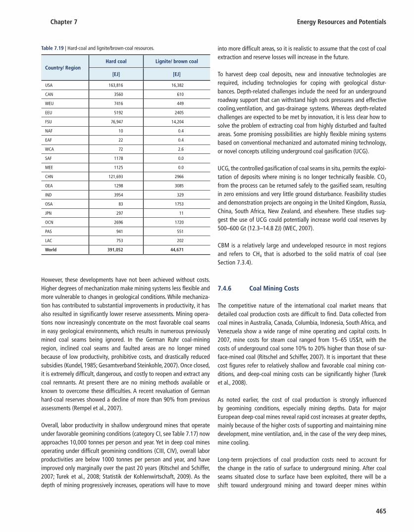
Chapter 7 Energy Resources and Potentials
465
However, these developments have not been achieved without costs. Higher degrees of mechanization make mining systems less flexible and more vulnerable to changes in geological conditions. While mechaniza-tion has contributed to substantial improvements in productivity, it has also resulted in significantly lower reserve assessments. Mining opera-tions now increasingly concentrate on the most favorable coal seams in easy geological environments, which results in numerous previously mined coal seams being ignored. In the German Ruhr coal-mining region, inclined coal seams and faulted areas are no longer mined because of low productivity, prohibitive costs, and drastically reduced subsidies (Kundel, 1985 ; Gesamtverband Steinkohle, 2007 ). Once closed, it is extremely difficult, dangerous, and costly to reopen and extract any coal remnants. At present there are no mining methods available or known to overcome these difficulties. A recent revaluation of German hard-coal reserves showed a decline of more than 90% from previous assessments (Rempel et al., 2007 ).
Overall, labor productivity in shallow underground mines that operate under favorable geomining conditions (category CI, see Table 7.17 ) now approaches 10,000 tonnes per person and year. Yet in deep coal mines operating under difficult geomining conditions (CIII, CIV), overall labor productivities are below 1000 tonnes per person and year, and have improved only marginally over the past 20 years (Ritschel and Schiffer, 2007 ; Turek et al., 2008 ; Statistik der Kohlenwirtschaft, 2009 ). As the depth of mining progressively increases, operations will have to move
into more difficult areas, so it is realistic to assume that the cost of coal extraction and reserve losses will increase in the future.
To harvest deep coal deposits, new and innovative technologies are required, including technologies for coping with geological distur-bances. Depth-related challenges include the need for an underground roadway support that can withstand high rock pressures and effective cooling,ventilation, and gas-drainage systems. Whereas depth-related challenges are expected to be met by innovation, it is less clear how to solve the problem of extracting coal from highly disturbed and faulted areas. Some promising possibilities are highly flexible mining systems based on conventional mechanized and automated mining technology, or novel concepts utilizing underground coal gasification (UCG).
UCG, the controlled gasification of coal seams in situ, permits the exploi-tation of deposits where mining is no longer technically feasible. CO 2 from the process can be returned safely to the gasified seam, resulting in zero emissions and very little ground disturbance. Feasibility studies and demonstration projects are ongoing in the United Kingdom, Russia, China, South Africa, New Zealand, and elsewhere. These studies sug-gest the use of UCG could potentially increase world coal reserves by 500–600 Gt (12.3–14.8 ZJ) (WEC, 2007 ).
CBM is a relatively large and undeveloped resource in most regions and refers to CH 4 that is adsorbed to the solid matrix of coal (see Section 7.3.4 ).
7.4.6 Coal Mining Costs
The competitive nature of the international coal market means that detailed coal production costs are difficult to find. Data collected from coal mines in Australia, Canada, Columbia, Indonesia, South Africa, and Venezuela show a wide range of mine operating and capital costs. In 2007 , mine costs for steam coal ranged from 15–65 US$/t, with the costs of underground coal some 10% to 20% higher than those of sur-face-mined coal (Ritschel and Schiffer, 2007 ). It is important that these cost figures refer to relatively shallow and favorable coal mining con-ditions, and deep-coal mining costs can be significantly higher (Turek et al., 2008 ).
As noted earlier, the cost of coal production is strongly influenced by geomining conditions, especially mining depths. Data for major European deep-coal mines reveal rapid cost increases at greater depths, mainly because of the higher costs of supporting and maintaining mine development, mine ventilation, and, in the case of the very deep mines, mine cooling.
Long-term projections of coal production costs need to account for the change in the ratio of surface to underground mining. After coal seams situated close to surface have been exploited, there will be a shift toward underground mining and toward deeper mines within
Table 7.19 | Hard-coal and lignite/brown-coal resources.
Country/ RegionHard coal Lignite/ brown coal
[EJ] [EJ]
USA 163,816 16,382
CAN 3560 610
WEU 7416 449
EEU 5192 2405
FSU 76,947 14,204
NAF 10 0.4
EAF 22 0.4
WCA 72 2.6
SAF 1178 0.0
MEE 1125 0.0
CHN 121,693 2966
OEA 1298 3085
IND 3954 329
OSA 83 1753
JPN 297 11
OCN 2696 1720
PAS 941 551
LAC 753 202
World 391,052 44,671
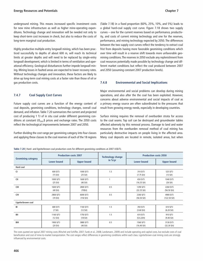
Energy Resources and Potentials Chapter 7
466
underground mining. This means increased specific investment costs for new mine infrastructure as well as higher mine-operating expen-ditures. Technology change and innovation will be needed not only to keep short-term cost increases in check, but also to reduce the costs of long-term marginal coal production.
Highly productive multiple-entry longwall mining, which has been prac-ticed successfully to depths of about 600 m, will reach its technical limits at greater depths and will need to be replaced by single-entry longwall development, which is limited in terms of ventilation and oper-ational efficiency. Geological disturbances further impede longwall min-ing. Mining losses in faulted areas are expected to lower recovery rates. Without technology changes and innovation, these factors are likely to drive up long-term coal mining costs at a faster rate than those of oil or gas production costs.
7.4.7 Coal Supply Cost Curves
Future supply cost curves are a function of the energy content of coal deposits, geomining conditions, technology changes, overall coal demand, and inflation. Table 7.20 summarizes the current and projected cost of producing 1 TJ of in situ coal under different geomining con-ditions at constant US 2007 $ prices and exchange rates. The 2050 costs reflect the technological improvements between 2007 and 2050.
Further dividing the cost range per geomining category into four classes and applying these classes to the coal reserves of each of the 18 regions
( Table 7.18 ) in a fixed proportion (60%, 25%, 10%, and 5%) leads to a global hard-coal supply cost curve. Figure 7.18 shows two supply curves – one for the current reserves based on performance, productiv-ity, and costs of current mining technology and one for the reserves, performance, and mining technology expected by 2050. The differences between the two supply cost curves reflect the tendency to extract coal frist from deposits having more favorable geomining conditions which over time will result in a reserve shift towards more unfavorable geo-mining conditions. The reserves in 2050 exclude any replenishment from coal resources potentially made possible by technology change and dif-ferent market conditions but reflect the coal produced between 2007 and 2050 (assuming constant 2007 production levels).
7.4.8 Environmental and Social Implications
Major environmental and social problems can develop during mining operations, and also after the the coal has been exploited. However, concerns about adverse environmental and social impacts of coal as a primary energy source are often subordinated to the pressures that result from growing energy needs, especially in developing countries.
Surface mining requires the removal of overburden strata for access to the coal seams. Top soil can be destroyed and groundwater tables affected adversely by this removal process. Damage to land and water resources from the overburden removal method of coal mining has particularly destructive impacts on people living in the affected area. Many coal deposits are located in remote, isolated areas, but when
Table 7.20 | Hard- and lignite/brown-coal production costs for different geomining conditions at 2007 US$/TJ.
Geomining category Production costs 2007
Technology change in %/yr
Production costs 2050
Lower bound Upper bound Lower bound Upper bound
Hard coal
CI 600 $/TJ (15 $/t)
1000 $/TJ (25 $/t)
1.5 310 $/TJ (7.75 $/t)
525 $/TJ (13 $/t)
CII 1000 $/TJ (25 $/t)
1600 $/TJ (40 $/t)
1 650 $/TJ (16.25 $/t)
1040 $/TJ (26 $/t)
CIII 1600 $/TJ (40 $/t)
2800 $/TJ (70$/t)
0.5 1290 $/TJ (32.25 $/t)
2260 $/TJ (56.50 $/t)
CIV 2800 $/TJ (70 $/t)
6000 $/TJ (150 $/t)
0.5 2260 $/TJ (56.50 $/t)
4900 $/TJ (122.50 $/t)
Lignite/brown coal
BI 680 $/TJ (7 $/t)
1160 $/TJ (12 $/t)
1.5 350 $/TJ (3.60 $/t)
610 $/TJ(6.20 $/t)
BII 1160 $/TJ (12 $/t)
1750 $/TJ (18 $/t)
1.5 610 $/TJ ($ 6.20/t)
910 $/TJ (9.40 $/t)
BIII 1900 $/TJ (20 $/t)
3880 $/TJ (40 $/t)
0.5 1560 $/TJ (16.40 $/t)
3130 $/TJ (32.30 $/t)
The costs quoted are typical 2007 mining costs (Ritschel and Schiffer, 2007 ; Turek et al., 2008 ; Landsmann, 2009 ) and include operating and capital costs, but exclude costs of coal benefi cation and cost of mine-to-market transportation. The cost ranges refl ect differences in geomining conditions within each class. Lignite/brown-coal mining costs are strongly infl uenced by environmental costs.

Chapter 7 Energy Resources and Potentials
467
mining operations are undertaken in densely populated areas, resettle-ment of the population can be a costly and politically sensitive issue. Differences in the cost of lignite mining in Europe and overseas are, to a considerable degree, linked to environmental legislation and the cost of resettlement.
Other environmental impacts of surface mining are ground vibrations and dust caused by overburden blasting. Once production has ceased, the overburden strata is returned to fill the void created by the coal extraction and the land surface is reshaped and rehabilitated. Many jurisdictions mandate rehabilitation to conditions at least equal to those prior to mining operations. As a result, the cost of land rehabilitation can be 20–30% of total mining cost and depends on climatic conditions, prior land use, and applicable mining regulations.
Underground coal mining is generally associated with less-severe environmental impacts, but presents significant health and safety hazards for workers, including mine fires, CH 4 and coal dust explo-sions, ground instability, and flooding. Coal mining requires a well-qualified and highly specialized workforce. In many countries such skills are not sufficiently available. Training and education of coal-mining personnel and continued mining R&D are essential as the extraction of deep coal resources in difficult geological environments requires new mining systems and technologies. With the demise of the nationalized coal-mining industries in most countries, mining research is left to equipment manufacturers and academic institu-tions (Wagner and Fettweis, 2001 ). As a result, research of coal-mine safety has suffered.
Mine subsidence is a critical issue. In the case of room and pillar mining, subsidence is a distinct possibility even many years after completion of mining operations. Caving of the roof strata tends to be less critical with longwall mining, particularly at great mine depths and moderate seam thicknesses. Mine subsidence associated with longwall mining is rather predictable and can be prevented by appropriate engineering
approaches. In sensitive areas, mine subsidence can be minimized by applying backfill (stowing).
Mine fires in relatively shallow underground mines can cause major environmental and safety hazards, especially where the sulfur content of coal is high. These fires can develop many years after completion of coal mining operations as a result of air entering through fractures in the overburden strata. Control of mine fires has been a serious chal-lenge in many mining countries, notably China. High sulfur contents in coal seams can also give rise to problems of acidic mine drainage.
Many coal resources in the northern hemisphere are located in areas of permafrost. This creates unique environmental problems that not only impact the environment, but also can give rise to unique technical and social problems. Other environmental concerns include CH 4 emissions from shallow coal-mine workings, and transportation of coal from the remote mining areas to the industrialized areas.
7.4.9 Summary
Proven hard- and lignite/brown-coal reserves are abundant, i.e., 21,000 EJ, of which 18,000 EJ are hard coal. Estimated coal resources exceed proven reserves more than 20 times. Even on the basis of a very conservative assumption of a 20% in situ recovery rate, coal is suffi-ciently available to support annual coal production increases of 2% for more than 100 years. However, many coal deposits are located in remote areas with little or no infrastructure and often harsh climatic conditions. Bringing these coals to the market will pose immense challenges.
Coal mining technology and productivity have increased significantly in recent years and secured the position of coal as the fossil energy source of lowest cost. The expected increase in the average depth of coal min-ing and increased environmental regulation of coal mining operations will exert upward pressure on production costs, while advances in min-ing technology are expected to at least partly offset these increased costs.
0
1
2
3
4
5
6
7
0 2000 4000 6000 8000 10,000 12,000 14,000 16,000 18,000 20,000
US$
(200
7) p
er G
J
EJ
0
1
2
3
4
5
6
7
0 500 1000 1500 2000 2500 3000 3500
US$
(200
7) p
er G
J
EJ
Current Technology
2050 TechnologyCurrent Technology
2050 Technology
Figure 7.18 | Global coal supply cost curves 12 for 2007 and 2050.
12 See footnote 7.
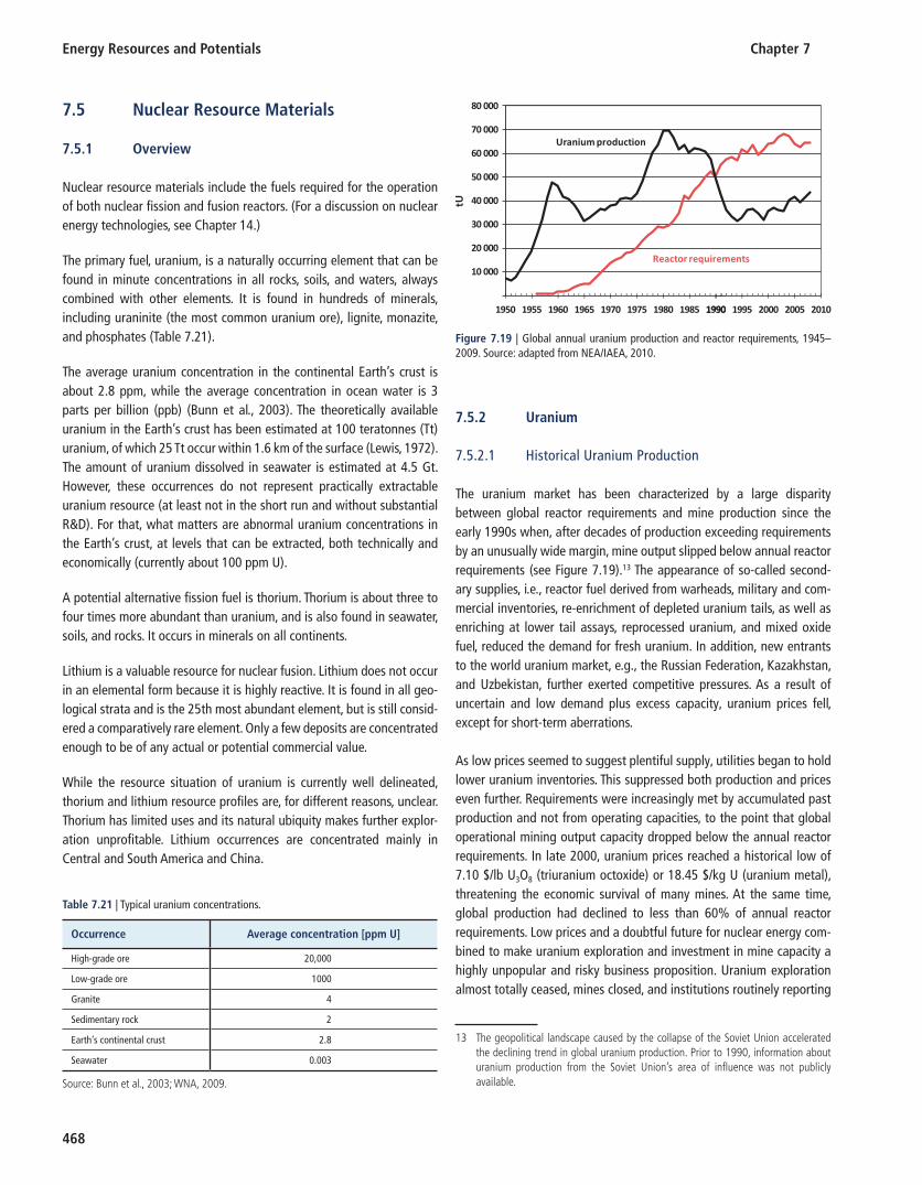
Energy Resources and Potentials Chapter 7
468
7.5 Nuclear Resource Materials
7.5.1 Overview
Nuclear resource materials include the fuels required for the operation of both nuclear fission and fusion reactors. (For a discussion on nuclear energy technologies, see Chapter 14 .)
The primary fuel, uranium, is a naturally occurring element that can be found in minute concentrations in all rocks, soils, and waters, always combined with other elements. It is found in hundreds of minerals, including uraninite (the most common uranium ore), lignite, monazite, and phosphates ( Table 7.21 ).
The average uranium concentration in the continental Earth’s crust is about 2.8 ppm, while the average concentration in ocean water is 3 parts per billion (ppb) (Bunn et al., 2003 ). The theoretically available uranium in the Earth’s crust has been estimated at 100 teratonnes (Tt) uranium, of which 25 Tt occur within 1.6 km of the surface (Lewis, 1972 ). The amount of uranium dissolved in seawater is estimated at 4.5 Gt. However, these occurrences do not represent practically extractable uranium resource (at least not in the short run and without substantial R&D). For that, what matters are abnormal uranium concentrations in the Earth’s crust, at levels that can be extracted, both technically and economically (currently about 100 ppm U).
A potential alternative fission fuel is thorium. Thorium is about three to four times more abundant than uranium, and is also found in seawater, soils, and rocks. It occurs in minerals on all continents.
Lithium is a valuable resource for nuclear fusion. Lithium does not occur in an elemental form because it is highly reactive. It is found in all geo-logical strata and is the 25th most abundant element, but is still consid-ered a comparatively rare element. Only a few deposits are concentrated enough to be of any actual or potential commercial value.
While the resource situation of uranium is currently well delineated, thorium and lithium resource profiles are, for different reasons, unclear. Thorium has limited uses and its natural ubiquity makes further explor-ation unprofitable. Lithium occurrences are concentrated mainly in Central and South America and China.
7.5.2 Uranium
7.5.2.1 Historical Uranium Production
The uranium market has been characterized by a large disparity between global reactor requirements and mine production since the early 1990s when, after decades of production exceeding requirements by an unusually wide margin, mine output slipped below annual reactor requirements (see Figure 7.19 ). 13 The appearance of so-called second-ary supplies, i.e., reactor fuel derived from warheads, military and com-mercial inventories, re-enrichment of depleted uranium tails, as well as enriching at lower tail assays, reprocessed uranium, and mixed oxide fuel, reduced the demand for fresh uranium. In addition, new entrants to the world uranium market, e.g., the Russian Federation, Kazakhstan, and Uzbekistan, further exerted competitive pressures. As a result of uncertain and low demand plus excess capacity, uranium prices fell, except for short-term aberrations.
As low prices seemed to suggest plentiful supply, utilities began to hold lower uranium inventories. This suppressed both production and prices even further. Requirements were increasingly met by accumulated past production and not from operating capacities, to the point that global operational mining output capacity dropped below the annual reactor requirements. In late 2000, uranium prices reached a historical low of 7.10 $/lb U 3 O 8 (triuranium octoxide) or 18.45 $/kg U (uranium metal), threatening the economic survival of many mines. At the same time, global production had declined to less than 60% of annual reactor requirements. Low prices and a doubtful future for nuclear energy com-bined to make uranium exploration and investment in mine capacity a highly unpopular and risky business proposition. Uranium exploration almost totally ceased, mines closed, and institutions routinely reporting
Table 7.21 | Typical uranium concentrations.
Occurrence Average concentration [ppm U]
High-grade ore 20,000
Low-grade ore 1000
Granite 4
Sedimentary rock 2
Earth’s continental crust 2.8
Seawater 0.003
Source: Bunn et al., 2003 ; WNA, 2009 .
13 The geopolitical landscape caused by the collapse of the Soviet Union accelerated the declining trend in global uranium production. Prior to 1990, information about uranium production from the Soviet Union’s area of infl uence was not publicly available.
Figure 7.19 | Global annual uranium production and reactor requirements, 1945–2009. Source: adapted from NEA/IAEA, 2010 .

Chapter 7 Energy Resources and Potentials
469
uranium reserves and resources became reluctant to do so in a compre-hensive manner.
The situation changed dramatically starting in 2000 for four main rea-sons. First, the license extension of nuclear power plants in the United States generated another 20 years of unexpected uranium demand. Second, the emergence in the uranium market of China and India, potentially major customers for uranium, generated additional demand with consequent pressure on supply capacity.
Third, in the light of volatile fossil-energy prices, energy security concerns, and concerns about climate change, a growing number of countries began to reevaluate the nuclear option thus further adding to potential supply shortfalls. Fourth, when two of the world’s top producing mines greatly reduced output because of fire and flooding incidents, the supply/demand imbalance began to impact uranium markets (PCA, 2006 ). Spot prices instantly shot through the roof and continued climbing, approach-ing 350 $/kgU in 2007 . Exploration expenditures also increased by an order of magnitude, from US$100 million in 2002 to over US$1 billion in 2008 . By April 2009 spot prices had dropped to one-third of the peak level or about 110 $/kgU and have not changed markedly since.
7.5.2.2 Conventional Uranium Reserves and Resources
Conventional uranium resources are defined as those occurrences from which uranium is recoverable as a primary product, a co-product, or an important by-product. Uranium reserves are periodically estimated by the OECD’s Nuclear Energy Agency (NEA) together with the International Atomic Energy Agency (IAEA), and also the World Nuclear Association (WNA), WEC, and numerous national geological institutions. NEA-IAEA estimates have the widest coverage, so the reserves reported in their lat-est survey (the so-called Red Book) are given here (NEA/IAEA, 2010 ). The two organizations define ‘reserves’ as those deposits that could be pro-duced competitively in an expanding market. This category is called iden-tified resources 14 and, until 2008, included uranium recoverable at less than 130 $/kgU. Stimulated by high spot prices of up to 350 $/kg in 2007, the 2010 edition of the Red Book extended the cost ranges to 260 $/kgU.
What is important for a good comprehension of the long-term availabil-ity of uranium is the impact of demand prospects and prices on the vol-ume of reported reserves and resources. The recent uranium-price hike stimulated exploration, prompted institutions to report occurrences long labeled irrelevant, and led companies to consider reopening high-cost mines. The RAR category in the Red Books increased by 27% between 2001 and 2009 (or 43% if reserves up to 260 $/kg production cost are included). In addition, the category of ‘uranium that could be expected
to be found based on the geological characteristics of known resources grew by 5%. Figure 7.20 shows the historical development of identified resources since the early 1970s.
Table 7.22 shows the identified uranium resources by region reported in the Red Book 2009 (NEA/IAEA, 2010 ). Altogether, there are 6.3 MtU (or 3.7 ZJ) 15 of conventional uranium resources available at extraction costs of less than 260 $/kgU. Vast additional uranium occurrences can be mobilized at costs larger than 260 $/kg.
Table 7.23 shows uranium occurrences yet to be discovered based on knowledge derived from already discovered and delineated deposits, as well as from regional geological analogies and mapping activities. Reports on ‘prognosticated resources’ are usually supported by some hard evi-dence. These deposits are generally located in known uranium provinces. Data on ‘speculative resources’ are not supported by direct evidence, but rather based on analogy and other considerations. Hence both categories require substantial additional exploration efforts before their existence can be confirmed and their overall qualities and quantities delineated.
Reporting on undiscovered resources ( Table 7.23 ) is sketchy and incom-plete, and recently the number of reporting countries has declined. Several reasons account for this decline, including funding constraints from governmental offices, lack of interest from industries, and plentiful known and accessible uranium occurrences.
7.5.2.3 Unconventional Uranium Resources
The distinction between conventional and unconventional resources is not clearly defined, but generally unconventional uranium resources
14 Until 2003 ‘Identifi ed Resources’ were reported as known conventional resources (KCR), i.e., the sum of reasonably assured resources (RAR) and estimated additional resources category-I (EAR-I). After 2003 Identifi ed resources are the sum of RAR and inferred resources.
Figure 7.20 | Development of identifi ed uranium resources at less than 130 $/kgU production costs, 1973–2009, and less than 260 $/kgU for 2009. Source: NEA/IAEA, 2010 .
15 The thermal energy equivalent of 1 tonne of uranium in average once-through fuel cycles is about 589 TJ (IPCC, 1996 ).
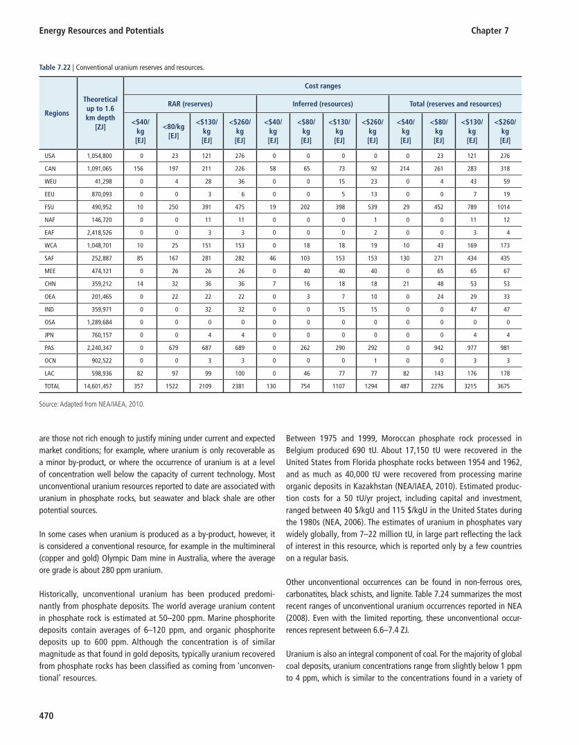
Energy Resources and Potentials Chapter 7
470
are those not rich enough to justify mining under current and expected market conditions; for example, where uranium is only recoverable as a minor by-product, or where the occurrence of uranium is at a level of concentration well below the capacity of current technology. Most unconventional uranium resources reported to date are associated with uranium in phosphate rocks, but seawater and black shale are other potential sources.
In some cases when uranium is produced as a by-product, however, it is considered a conventional resource, for example in the multimineral (copper and gold) Olympic Dam mine in Australia, where the average ore grade is about 280 ppm uranium.
Historically, unconventional uranium has been produced predomi-nantly from phosphate deposits. The world average uranium content in phosphate rock is estimated at 50–200 ppm. Marine phosphorite deposits contain averages of 6–120 ppm, and organic phosphorite deposits up to 600 ppm. Although the concentration is of similar magnitude as that found in gold deposits, typically uranium recovered from phosphate rocks has been classified as coming from ‘unconven-tional’ resources.
Between 1975 and 1999, Moroccan phosphate rock processed in Belgium produced 690 tU. About 17,150 tU were recovered in the United States from Florida phosphate rocks between 1954 and 1962, and as much as 40,000 tU were recovered from processing marine organic deposits in Kazakhstan (NEA/IAEA, 2010 ). Estimated produc-tion costs for a 50 tU/yr project, including capital and investment, ranged between 40 $/kgU and 115 $/kgU in the United States during the 1980s (NEA, 2006 ). The estimates of uranium in phosphates vary widely globally, from 7–22 million tU, in large part reflecting the lack of interest in this resource, which is reported only by a few countries on a regular basis.
Other unconventional occurrences can be found in non-ferrous ores, carbonatites, black schists, and lignite. Table 7.24 summarizes the most recent ranges of unconventional uranium occurrences reported in NEA (2008). Even with the limited reporting, these unconventional occur-rences represent between 6.6–7.4 ZJ.
Uranium is also an integral component of coal. For the majority of global coal deposits, uranium concentrations range from slightly below 1 ppm to 4 ppm, which is similar to the concentrations found in a variety of
Table 7.22 | Conventional uranium reserves and resources.
Regions
Theoretical up to 1.6 km depth
[ZJ]
Cost ranges
RAR (reserves) Inferred (resources) Total (reserves and resources)
<$40/kg [EJ]
<80/kg [EJ]
<$130/kg [EJ]
<$260/kg [EJ]
<$40/kg [EJ]
<$80/kg [EJ]
<$130/kg [EJ]
<$260/kg [EJ]
<$40/kg [EJ]
<$80/kg [EJ]
<$130/kg [EJ]
<$260/kg [EJ]
USA 1,054,800 0 23 121 276 0 0 0 0 0 23 121 276
CAN 1,091,065 156 197 211 226 58 65 73 92 214 261 283 318
WEU 41,298 0 4 28 36 0 0 15 23 0 4 43 59
EEU 870,093 0 0 3 6 0 0 5 13 0 0 7 19
FSU 490,952 10 250 391 475 19 202 398 539 29 452 789 1014
NAF 146,720 0 0 11 11 0 0 0 1 0 0 11 12
EAF 2,418,526 0 0 3 3 0 0 0 2 0 0 3 4
WCA 1,048,701 10 25 151 153 0 18 18 19 10 43 169 173
SAF 252,887 85 167 281 282 46 103 153 153 130 271 434 435
MEE 474,121 0 26 26 26 0 40 40 40 0 65 65 67
CHN 359,212 14 32 36 36 7 16 18 18 21 48 53 53
OEA 201,465 0 22 22 22 0 3 7 10 0 24 29 33
IND 359,971 0 0 32 32 0 0 15 15 0 0 47 47
OSA 1,289,684 0 0 0 0 0 0 0 0 0 0 0 0
JPN 760,157 0 0 4 4 0 0 0 0 0 0 4 4
PAS 2,240,347 0 679 687 689 0 262 290 292 0 942 977 981
OCN 902,522 0 0 3 3 0 0 0 1 0 0 3 3
LAC 598,936 82 97 99 100 0 46 77 77 82 143 176 178
TOTAL 14,601,457 357 1522 2109 2381 130 754 1107 1294 487 2276 3215 3675
Source: Adapted from NEA/IAEA, 2010 .

Chapter 7 Energy Resources and Potentials
471
common rocks and soils (see Table 7.21 ). Since uranium is not combusti-ble, it remains in the ash at concentrations ten times and more than that in the original coal. Current global electricity-generation accumulates on average 3400 tU in the ashes per year.
Of specific interest are the ashes from lignite-burning coal plants located in areas where the lignite resources contain higher than normal levels of uranium. For example, the fly ash at the Xiaolongtang coal power plant in Yunnan Province, China, averages 160–180 ppm, which is only about a quarter of the concentration considered commercially viable for uran-ium extraction by in situ leaching (ISL), a conventional mining and extrac-tion process. However, coal-ash piles are easier to drill in. In addition, it may be easier to protect local groundwater from contamination. There might also be some monetary value in reducing coal-ash radiotoxicity if regulatory requirements restrict the ash use or require its cleanup. The cumulative ash volume at the Xiaolongtang site is estimated at 5.3 Mt, and contains between 850–950 tU.
Seawater is also a possible unconventional source of uranium. The total mass of uranium in seawater is enormous and amounts to about 4.5 GtU, dwarfing any other exhaustible energy resource. However, because of the low concentration level (3–4 ppb), it is estimated that processing of about 350,000 tonnes of water would be required to produce one kilogram
of uranium. In the 1970s and 1980s, recovery from seawater was on the agenda of several countries. Today research is effectively ongoing only in Japan and France. A braid-type recovery system directly moored to the ocean floor recovered about 1.5 g U over a 30-day test period (Tamada et al., 2006 ; 2009 ), but the recovery costs of such a system are over 700 $/kgU, several times the current market price (NEA/IAEA, 2008 ). Other studies quote recovery costs between 260 $/kgU and 1700 $/kgU (Nobukawa et al., 1994 ; Kato et al., 1999 ; Bunn et al., 2003 ).
“The performance of current [uranium] adsorbents is highly dependent on temperature, and they are thus effectively limited to warm surface waters. However, horizontal and vertical mixing of the ocean would make seawater uranium accessible in warm surface waters at essen-tially constant concentrations for many centuries, so long as the rate of extraction did not exceed ~2 MtU/yr (30 times current global reactor requirements)” (Bunn et al., 2003 ).
These cost estimates for uranium from seawater do not include the value of the other metals (vanadium, cobalt, titanium, molybdenum) that would be co-recovered with the uranium (Sugo et al., 2001 ). Depending on the future long-term market prices of these co-recovered materials, their values might be sufficient to reduce substantially the net uranium recovery cost per kilogram of uranium.
Table 7.23 | Undiscovered conventional uranium occurrences.
Regions
Prognosticated resources
<$80/kgU [EJ]
<$130/kgU [EJ]
Total prognostic and speculative
[EJ]
Unconventional [EJ]
USA 490 744 744 501 501 282 1526 2642
CAN 29 88 88 409 409 0 496 0
WEU 4 4 4 29 29 55 88 183
EEU 0 28 28 2 2 105 134 0
FSU 221 456 457 158 245 527 1229 34
NAF 0 0 0 0 0 0 0 3890
EAF 0 0 0 0 0 0 0 0
WCA 8 14 14 0 0 0 14 0
SAF 20 77 77 15 15 650 742 0
MEE 40 52 52 50 58 0 110 106
CHN 2 2 2 2 2 0 4 0
OEA 0 5 5 870 870 76 951 0
IND 0 0 37 0 0 10 47 10
OSA 0 0 0 0 0 0 0 0
JPN 0 0 0 0 0 0 0 0
OCN 0 0 0 0 0 0 0 0
PAS 0 0 0 9 9 0 9 1
LAC 179 197 197 138 138 398 733 156
TOTAL 994 1666 1705 2183 2279 2102 6086 7022
Source: adapted from NEA/IAEA, 2010 .
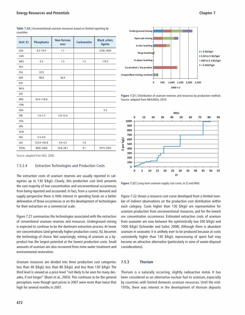
Energy Resources and Potentials Chapter 7
472
7.5.2.4 Extraction Technologies and Production Costs
The extraction costs of uranium reserves are usually reported in cat-egories up to 130 $/kgU. Clearly, this production cost limit prevents the vast majority of low concentration and unconventional occurrences from being reported and accounted. In fact, from a current demand and supply perspective there is little interest in spending funds on a better delineation of these occurrences or on the development of technologies for their extraction on a commercial scale.
Figure 7.21 summarizes the technologies associated with the extraction of conventional uranium reserves and resources. Underground mining is expected to continue to be the dominant extraction process. At lower ore concentrations (and generally higher production costs), ISL becomes the technology of choice. Not surprisingly, mining of uranium as a by-product has the largest potential at the lowest production costs. Small amounts of uranium are also recovered from mine-water treatment and environmental restoration.
Uranium resources are divided into three production cost categories: less than 40 $/kgU, less than 80 $/kgU, and less than 130 $/kgU. The third level is viewed as a price level “not likely to be seen for many dec-ades, if not longer” (Bunn et al., 2003 ). This continues to be the general perception, even though spot prices in 2007 were more than twice that high for several months in 2007.
Figure 7.22 shows a resource cost curve developed from a limited num-ber of indirect observations on the production cost distribution within each category. Costs higher than 130 $/kgU are representative for uranium production from unconventional resources, and for the lowest ore concentration occurrences. Estimated extraction costs of uranium from seawater are now between the optimistically low 200 $/kgU and 1000 $/kgU (Schneider and Sailor, 2008 ). Although there is abundant uranium in seawater, it is unlikely ever to be produced because at costs consistently higher than 130 $/kgU, reprocessing of spent fuel may become an attractive alternative (particularly in view of waste-disposal considerations).
7.5.3 Thorium
Thorium is a naturally occurring, slightly radioactive metal. It has been considered as an alternative nuclear fuel to uranium, especially by countries with limited domestic uranium resources. Until the mid-1970s, there was interest in the development of thorium deposits
Table 7.24 | Unconventional uranium resources based on limited reporting by countries.
Unit: EJ PhosphatesNon-ferrous
oresCarbonatite
Black schist, lignite
USA 8.2–19.3 1.1 2336–2920
CAN
WEU 0.3 1.5 1.5 179.3
EEU
FSU 33.9
NAF 3832 58.4
EAF
WCA
SAF
MEE 93.4–118.8
CHN
OEA 0.3
IND 1.0–1.5 3.9–13.4
OSA
JPN
OCN
PAS 0.3–0.9
LAC 123.0–165.8 3.9–4.5 7.6
TOTAL 4092–4456 10.8–28.1 9.1 2515–2925
Source: adapted from NEA, 2006 .
0 500 1,000 1,500 2,000 2,500
Unspecified mining method
Co-product / by-product
In-place leaching
Heap leaching
In situ leaching
Open-pit mining
Underground mining
1000 t U
< $ 40/kgU
$ 40 to $ 80/kgU
$80 to $ 130/kgU
< $ 260/kgU
Figure 7.21 | Distribution of uranium reserves and resources by production method. Source: adapted from NEA/IAEA, 2010 .
0 10 20 30 40 50 60 70 80 90
0
100
200
300
400
500
600
700
800
900
1000
0 5 10 15 20 25 30 35 40 45 50 55
MtU
$ pe
r kg
U
ZJ
Figure 7.22 | Long-term uranium supply cost curve, in ZJ and MtU.
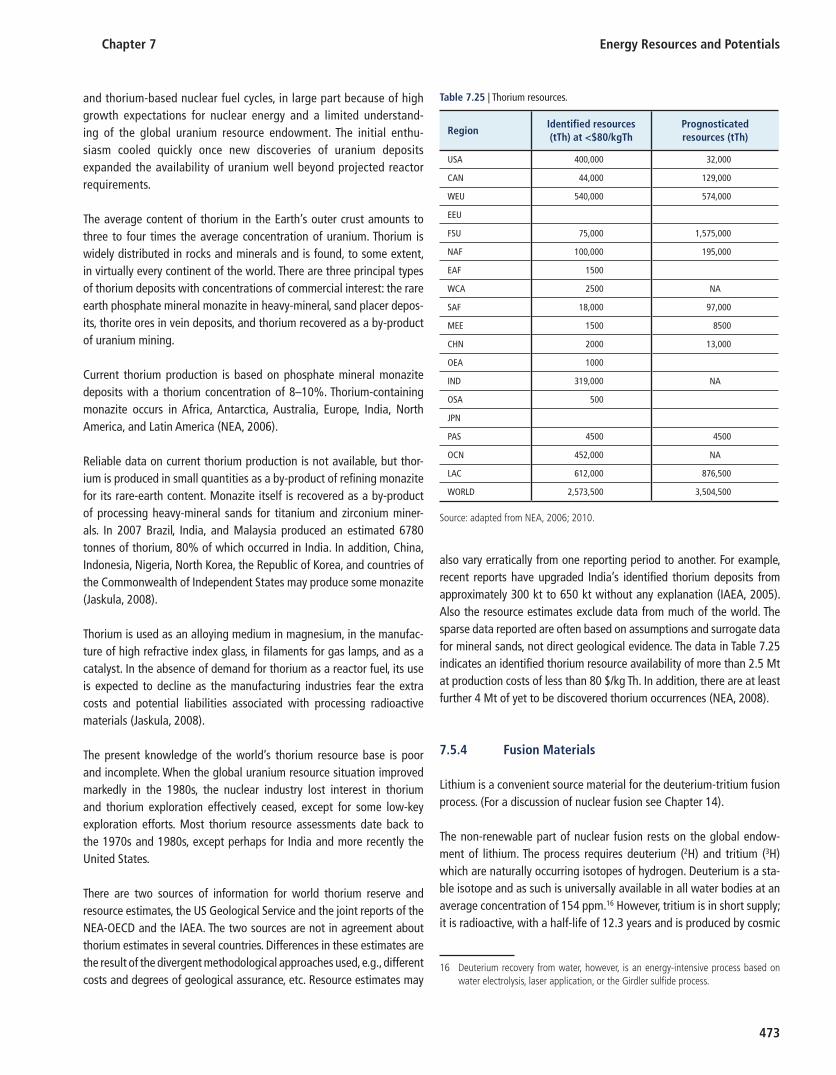
Chapter 7 Energy Resources and Potentials
473
and thorium-based nuclear fuel cycles, in large part because of high growth expectations for nuclear energy and a limited understand-ing of the global uranium resource endowment. The initial enthu-siasm cooled quickly once new discoveries of uranium deposits expanded the availability of uranium well beyond projected reactor requirements.
The average content of thorium in the Earth’s outer crust amounts to three to four times the average concentration of uranium. Thorium is widely distributed in rocks and minerals and is found, to some extent, in virtually every continent of the world. There are three principal types of thorium deposits with concentrations of commercial interest: the rare earth phosphate mineral monazite in heavy-mineral, sand placer depos-its, thorite ores in vein deposits, and thorium recovered as a by-product of uranium mining.
Current thorium production is based on phosphate mineral monazite deposits with a thorium concentration of 8–10%. Thorium-containing monazite occurs in Africa, Antarctica, Australia, Europe, India, North America, and Latin America (NEA, 2006 ).
Reliable data on current thorium production is not available, but thor-ium is produced in small quantities as a by-product of refining monazite for its rare-earth content. Monazite itself is recovered as a by-product of processing heavy-mineral sands for titanium and zirconium miner-als. In 2007 Brazil, India, and Malaysia produced an estimated 6780 tonnes of thorium, 80% of which occurred in India. In addition, China, Indonesia, Nigeria, North Korea, the Republic of Korea, and countries of the Commonwealth of Independent States may produce some monazite (Jaskula, 2008).
Thorium is used as an alloying medium in magnesium, in the manufac-ture of high refractive index glass, in filaments for gas lamps, and as a catalyst. In the absence of demand for thorium as a reactor fuel, its use is expected to decline as the manufacturing industries fear the extra costs and potential liabilities associated with processing radioactive materials (Jaskula, 2008).
The present knowledge of the world’s thorium resource base is poor and incomplete. When the global uranium resource situation improved markedly in the 1980s, the nuclear industry lost interest in thorium and thorium exploration effectively ceased, except for some low-key exploration efforts. Most thorium resource assessments date back to the 1970s and 1980s, except perhaps for India and more recently the United States.
There are two sources of information for world thorium reserve and resource estimates, the US Geological Service and the joint reports of the NEA-OECD and the IAEA. The two sources are not in agreement about thorium estimates in several countries. Differences in these estimates are the result of the divergent methodological approaches used, e.g., different costs and degrees of geological assurance, etc. Resource estimates may
also vary erratically from one reporting period to another. For example, recent reports have upgraded India’s identified thorium deposits from approximately 300 kt to 650 kt without any explanation (IAEA, 2005 ). Also the resource estimates exclude data from much of the world. The sparse data reported are often based on assumptions and surrogate data for mineral sands, not direct geological evidence. The data in Table 7.25 indicates an identified thorium resource availability of more than 2.5 Mt at production costs of less than 80 $/kg Th. In addition, there are at least further 4 Mt of yet to be discovered thorium occurrences (NEA, 2008).
7.5.4 Fusion Materials
Lithium is a convenient source material for the deuterium-tritium fusion process. (For a discussion of nuclear fusion see Chapter 14 ).
The non-renewable part of nuclear fusion rests on the global endow-ment of lithium. The process requires deuterium ( 2 H) and tritium ( 3 H) which are naturally occurring isotopes of hydrogen. Deuterium is a sta-ble isotope and as such is universally available in all water bodies at an average concentration of 154 ppm. 16 However, tritium is in short supply; it is radioactive, with a half-life of 12.3 years and is produced by cosmic
Table 7.25 | Thorium resources.
RegionIdentified resources (tTh) at <$80/kgTh
Prognosticated resources (tTh)
USA 400,000 32,000
CAN 44,000 129,000
WEU 540,000 574,000
EEU
FSU 75,000 1,575,000
NAF 100,000 195,000
EAF 1500
WCA 2500 NA
SAF 18,000 97,000
MEE 1500 8500
CHN 2000 13,000
OEA 1000
IND 319,000 NA
OSA 500
JPN
PAS 4500 4500
OCN 452,000 NA
LAC 612,000 876,500
WORLD 2,573,500 3,504,500
Source: adapted from NEA, 2006 ; 2010.
16 Deuterium recovery from water, however, is an energy-intensive process based on water electrolysis, laser application, or the Girdler sulfi de process.

Energy Resources and Potentials Chapter 7
474
rays interacting with gases in the atmosphere. Tritium can be bred from lithium by neutron capture within the fusion reactor in an exothermic reaction (Harms et al., 2000 ; IEA, 2006b ).
The availability of lithium, although more limited than that of deuterium, is still large enough to potentially supply the world’s energy demand for thousands of years (Ongena and Van Oost, 2004 ).
Lithium is used in a number of products and processes, such as batteries, ceramics, glass, aircraft alloys, pharmaceuticals, lubricants, and air con-ditioning. Its use in rechargeable batteries has expanded significantly in recent years, driven by portable electronic devices and electrical tools. Today, batteries for electric cars constitute the largest and fastest-grow-ing market for lithium compounds.
Lithium does not occur ‘free,’ i.e., purified or uncombined, in nature. It is found joined (ionized) in various salts in nearly all igneous rocks (espe-cially pegmatites), in sedimentary rocks, and hydrated in brines and in seawater. Brines constitute almost two-thirds of the world’s lithium resources, followed by pegmatites (26%).
In natural seawater, lithium is found hydrated at low levels, usually ranging from 140–250 ppb. Only near hydrothermal vents under the oceans does natural seawater contain elevated levels of lithium, where it approaches 7000 ppb. Altogether, an estimated 250 Gt of lithium dissolved in seawa-ter represents an enormous resource (Chitraka et al., 2001). Japan and South Korea lead the development of lithium recovery technology from seawater, but these technologies are in their infancy and lithium from seawater is thus not included in most resource estimations.
As in many resource estimations, lithium reserve and resource esti-mates vary wildly and lack consistency. Recent resource estimates vary between 22 Mt (Tahil, 2007 ) and 62 Mt (Yaksic and Tilton, 2009 ) of lith-ium globally, with the bulk located in Latin America (Bolivia and Chile account for more than 40% of global resources). The discrepancies typ-ically result from varying assumptions, methodologies, use of termin-ology, and inclusion of deposits.
Table 7.26 shows the geographical distribution of lithium, resources plus reserves, across the 18 GEA regions and at the same time shows the large range in estimations. It was necessary to combine reserve and resources in this table, as different authors use different definitions of reserves. Table 7.27 summarizes some of the reserve and resource estimations.
7.5.5 Environmental and Social Implications
Like all mining, uranium mining affects the environment and carries cer-tain risks. In many respects these are much the same as those of the min-ing of any other mineral and, like any other mineral, uranium has unique features that must be managed with regard to its specific properties.
One special property of uranium is its radioactive nature. Uranium is mildly radioactive comparable to the levels found in granite. Concern about radioactivity is not unique to uranium mining, but is also a feature of oil and gas production (radium and radon) or the mining of mineral sands (thorium). Although uranium itself is not very radioactive, the ore which is mined contains radium and radon and needs special attention to occupational health and safety protection. This is increasingly regu-lated by the International Organization for Standardization environmen-tal management system.
Table 7.27 | Estimations of lithium reserves and resources in megatonnes (Mt).
Reserves Reference Resources Reference
[Mt] [Mt]
6.8 Tahil ( 2007 ) 15 Tahil ( 2007 )
9.9 USGS ( 2010 ) 25.5 USGS ( 2010 )
24.9 Yaksic and Tilton ( 2009 )
29.9 Evans ( 2008 )
36.9 Yaksic and Tilton ( 2009 )
38.3 Gruber and Medina ( 2010 )
39.3 Clarke and Harben ( 2009 )
Table 7.26 | Estimates of lithium reserves plus resources in 1000 tonnes (kt).
Regions
Evans ( 2008 )
Tahil ( 2007 )
Yaksic and Tilton ( 2009 )
Clarke and Harben ( 2009 )
[kt] [kt] [kt] [kt]
USA 5940 450 5735 6620
CAN 260 540 375 1073
WEU 115 125 221
EEU 850 957
FSU 1000 1160 2480
NAF
EAF
WCA 2300 2325 1145
SAF 60 50 70 57
MEE 2000
CHN 3350 3800 5180 6173
OEA
IND
OSA
JPN
OCN 280 420 340 1603
PAS
LAC 15,600 16,700 44,515 19,043
Total 29,755 21,960 61,825 39,372

Chapter 7 Energy Resources and Potentials
475
Most of the radioactivity is in the tailings – the solid waste product left after uranium oxide has been extracted by milling of the uranium-bearing ore. Tailings include most of the original ore, including all the radium, and contain most of the radioactivity (WNA, 2009 ).The tailings are deposited in dam-like structures, and during mine operation the tail-ing dam is usually covered by water to confine surface radioactivity and radon emissions. After mine closure, the tailings are covered with clay, rock, topsoil, and vegetation. The radioactivity of the tailing is about 80–85% of the ore that initially contained the ore body (AUA, 2009 ) and the cover further reduces potential human exposure.
Run-off water from the mine stockpiles and process water from milling operations contain traces of radium and some other metals, hence this water needs to be prevented from entering biological systems. These liquids are collected in secure retention ponds for isolation and recov-ery of any heavy metals or other contaminants. The liquid portion is disposed of either by natural evaporation or recirculation to the milling operation. Several mines have begun to adopt a ‘zero discharge’ policy for any pollutants (WNA, 2009 ).
Historically, uranium production has principally involved open-pit and underground mining. However, over the past two decades, ISL min-ing, which uses either acid or alkaline solutions to extract the uranium directly from the deposit (the ore body stays in the ground), has become increasingly important. The uranium-dissolving solutions are injected into, and recovered from, the ore-bearing zone using a system of wells. In 2008 , production by ISL exceeded production by open-pit mining and a larger reliance on ISL is expected to continue.
The main environmental consideration with ISL is avoiding the contam-ination of any groundwater away from the ore body, and leaving the immediate groundwater no less useful than it was initially (WNA, 2009 ). Apart from groundwater considerations, rehabilitation of ISL mines is very straightforward and much easier to accomplish than that of open-pit mining, making this a technique with lower environmental impact. Upon decommissioning, wells are sealed or capped, process facilities are removed, and evaporation ponds revegetated (WNA, 2009 ).
7.5.6 Summary
Fissile material resources are plentiful and lack of resource occurrences does not limit the future expansion of nuclear energy. However, a lack of timely investment in exploration and new mining capacities can result in supply shortages and market price volatility, as witnessed in 2007 . A sudden shift in demand, such as the unexpected license exten-sions in the United States and elsewhere, can cause short-term aber-rations if uranium producers fail to plan accordingly. Unconventional uranium occurrences (i.e., low concentration ores) exist, but are only economically extractable as by-products of other mining processes, or from coal ash.
Thorium and lithium are both available in large quantities, but require more comprehensive resource assessments and explorations activities. Still, the development of extraction and processing technologies for their large-scale commercial production will only be undertaken if demand prospects warrant such investments. Lithium as a fuel for nuclear fusion will most likely be preceded by its use in batteries for electric vehicles, while thorium, although an alternative to uranium with great potential, will be considered by countries lacking natural endowments of uranium primarily.
7.6 Hydropower
7.6.1 Overview
Hydropower exploits the energy of falling or flowing water by convert-ing it into electricity. It is the most developed and mature renewable technology globally. Current electricity generation by hydropower uti-lizes some 12.8 EJ/yr of its potential and kinetic energy, from which 3208 TWh were produced in 2008. Hydropower accounts for about 16% of global electricity generation and over 90% of electricity from renew-able sources (IEA, 2010a ).
The global hydrological cycle is the result of solar energy evaporating water, with oceans having a larger evaporation per unit area than land. Winds transfer the water vapor from oceans to land through precipitation. A global water balance requires that the water pre-cipitated on land eventually returns to the oceans as run off through rivers.
Hydropower projects can be classified by either storage capacity or by purpose. These classifications, however, are not mutually exclusive (IEA, 2000 ). Run-of-river projects, which have limited storage capacity, gen-erate electricity according to the available hydrological fluctuations of the site. Reservoir-type projects involve damming water and creating reservoirs with significant storage capacity, which allows for the regula-tion of water flow and electricity production.
Hydropower resources may be designed for electricity generation alone, or for multiple purposes. Multipurpose projects typically have significant reservoir capacity and can provide services such as irrigation, freshwater supply, flood control, and recreation. These uses may affect the volume of water available for electricity generation. In fact, 30–40% of world irrigation is supplied by reservoirs (Lemp é ri è re, 2006). This can distort quantitative assessments of the economic potential of hydropower for energy purposes.
Pumped storage projects are used to provide efficient storage of energy, especially for intermittent renewable resources. As they do not generate net electricity, they are excluded from the assessment of hydropower potentials.
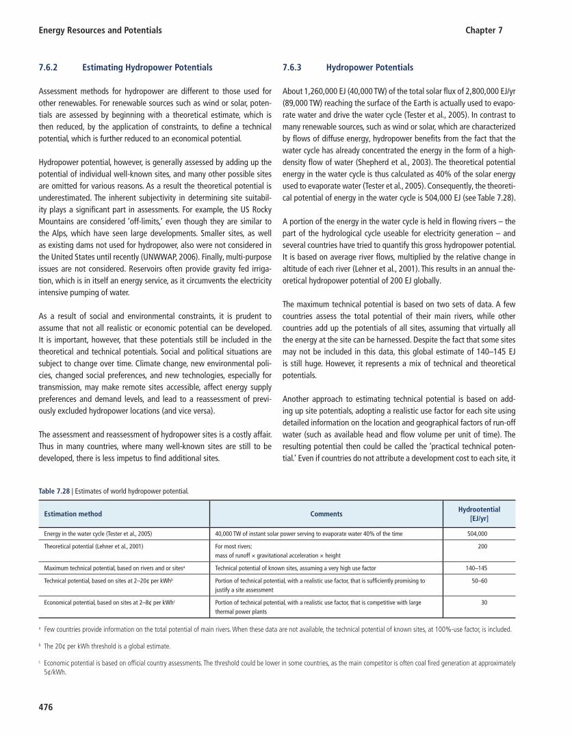
Energy Resources and Potentials Chapter 7
476
7.6.2 Estimating Hydropower Potentials
Assessment methods for hydropower are different to those used for other renewables. For renewable sources such as wind or solar, poten-tials are assessed by beginning with a theoretical estimate, which is then reduced, by the application of constraints, to define a technical potential, which is further reduced to an economical potential.
Hydropower potential, however, is generally assessed by adding up the potential of individual well-known sites, and many other possible sites are omitted for various reasons. As a result the theoretical potential is underestimated. The inherent subjectivity in determining site suitabil-ity plays a significant part in assessments. For example, the US Rocky Mountains are considered ‘off-limits,’ even though they are similar to the Alps, which have seen large developments. Smaller sites, as well as existing dams not used for hydropower, also were not considered in the United States until recently (UNWWAP, 2006 ). Finally, multi-purpose issues are not considered. Reservoirs often provide gravity fed irriga-tion, which is in itself an energy service, as it circumvents the electricity intensive pumping of water.
As a result of social and environmental constraints, it is prudent to assume that not all realistic or economic potential can be developed. It is important, however, that these potentials still be included in the theoretical and technical potentials. Social and political situations are subject to change over time. Climate change, new environmental poli-cies, changed social preferences, and new technologies, especially for transmission, may make remote sites accessible, affect energy supply preferences and demand levels, and lead to a reassessment of previ-ously excluded hydropower locations (and vice versa).
The assessment and reassessment of hydropower sites is a costly affair. Thus in many countries, where many well-known sites are still to be developed, there is less impetus to find additional sites.
7.6.3 Hydropower Potentials
About 1,260,000 EJ (40,000 TW) of the total solar flux of 2,800,000 EJ/yr (89,000 TW) reaching the surface of the Earth is actually used to evapo-rate water and drive the water cycle (Tester et al., 2005 ). In contrast to many renewable sources, such as wind or solar, which are characterized by flows of diffuse energy, hydropower benefits from the fact that the water cycle has already concentrated the energy in the form of a high-density flow of water (Shepherd et al., 2003 ). The theoretical potential energy in the water cycle is thus calculated as 40% of the solar energy used to evaporate water (Tester et al., 2005 ). Consequently, the theoreti-cal potential of energy in the water cycle is 504,000 EJ (see Table 7.28 ).
A portion of the energy in the water cycle is held in flowing rivers – the part of the hydrological cycle useable for electricity generation – and several countries have tried to quantify this gross hydropower potential. It is based on average river flows, multiplied by the relative change in altitude of each river (Lehner et al., 2001 ). This results in an annual the-oretical hydropower potential of 200 EJ globally.
The maximum technical potential is based on two sets of data. A few countries assess the total potential of their main rivers, while other countries add up the potentials of all sites, assuming that virtually all the energy at the site can be harnessed. Despite the fact that some sites may not be included in this data, this global estimate of 140–145 EJ is still huge. However, it represents a mix of technical and theoretical potentials.
Another approach to estimating technical potential is based on add-ing up site potentials, adopting a realistic use factor for each site using detailed information on the location and geographical factors of run-off water (such as available head and flow volume per unit of time). The resulting potential then could be called the ‘practical technical poten-tial.’ Even if countries do not attribute a development cost to each site, it
Table 7.28 | Estimates of world hydropower potential.
Estimation method Comments Hydrootential
[EJ/yr]
Energy in the water cycle (Tester et al., 2005 ) 40,000 TW of instant solar power serving to evaporate water 40% of the time 504,000
Theoretical potential (Lehner et al., 2001 ) For most rivers: mass of runoff × gravitational acceleration × height
200
Maximum technical potential, based on rivers and or sites a Technical potential of known sites, assuming a very high use factor 140–145
Technical potential, based on sites at 2–20¢ per kWh b Portion of technical potential, with a realistic use factor, that is suffi ciently promising to justify a site assessment
50–60
Economical potential, based on sites at 2–8¢ per kWh c Portion of technical potential, with a realistic use factor, that is competitive with large thermal power plants
30
a Few countries provide information on the total potential of main rivers. When these data are not available, the technical potential of known sites, at 100%-use factor, is included.
b The 20¢ per kWh threshold is a global estimate.
c Economic potential is based on offi cial country assessments. The threshold could be lower in some countries, as the main competitor is often coal fi red generation at approximately 5¢/kWh.
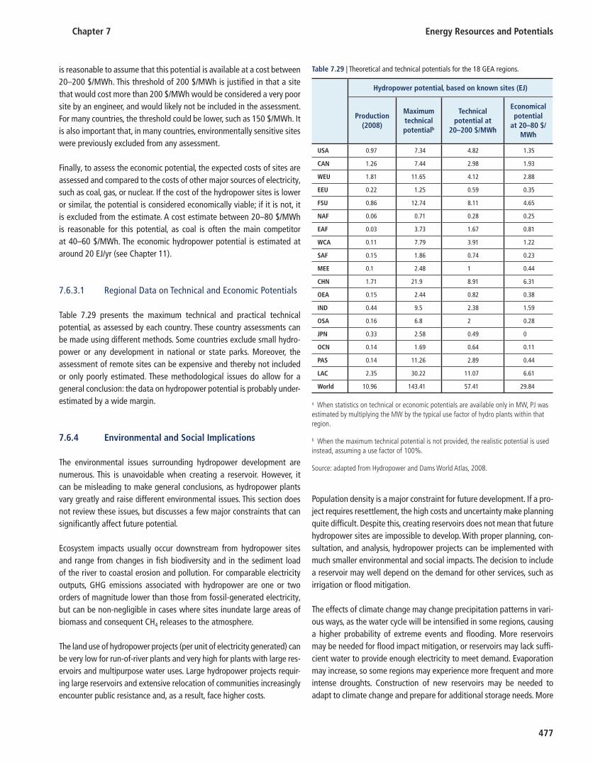
Chapter 7 Energy Resources and Potentials
477
is reasonable to assume that this potential is available at a cost between 20–200 $/MWh. This threshold of 200 $/MWh is justified in that a site that would cost more than 200 $/MWh would be considered a very poor site by an engineer, and would likely not be included in the assessment. For many countries, the threshold could be lower, such as 150 $/MWh. It is also important that, in many countries, environmentally sensitive sites were previously excluded from any assessment.
Finally, to assess the economic potential, the expected costs of sites are assessed and compared to the costs of other major sources of electricity, such as coal, gas, or nuclear. If the cost of the hydropower sites is lower or similar, the potential is considered economically viable; if it is not, it is excluded from the estimate. A cost estimate between 20–80 $/MWh is reasonable for this potential, as coal is often the main competitor at 40–60 $/MWh. The economic hydropower potential is estimated at around 20 EJ/yr (see Chapter 11 ).
7.6.3.1 Regional Data on Technical and Economic Potentials
Table 7.29 presents the maximum technical and practical technical potential, as assessed by each country. These country assessments can be made using different methods. Some countries exclude small hydro-power or any development in national or state parks. Moreover, the assessment of remote sites can be expensive and thereby not included or only poorly estimated. These methodological issues do allow for a general conclusion: the data on hydropower potential is probably under-estimated by a wide margin.
7.6.4 Environmental and Social Implications
The environmental issues surrounding hydropower development are numerous. This is unavoidable when creating a reservoir. However, it can be misleading to make general conclusions, as hydropower plants vary greatly and raise different environmental issues. This section does not review these issues, but discusses a few major constraints that can significantly affect future potential.
Ecosystem impacts usually occur downstream from hydropower sites and range from changes in fish biodiversity and in the sediment load of the river to coastal erosion and pollution. For comparable electricity outputs, GHG emissions associated with hydropower are one or two orders of magnitude lower than those from fossil-generated electricity, but can be non-negligible in cases where sites inundate large areas of biomass and consequent CH 4 releases to the atmosphere.
The land use of hydropower projects (per unit of electricity generated) can be very low for run-of-river plants and very high for plants with large res-ervoirs and multipurpose water uses. Large hydropower projects requir-ing large reservoirs and extensive relocation of communities increasingly encounter public resistance and, as a result, face higher costs.
Population density is a major constraint for future development. If a pro-ject requires resettlement, the high costs and uncertainty make planning quite difficult. Despite this, creating reservoirs does not mean that future hydropower sites are impossible to develop. With proper planning, con-sultation, and analysis, hydropower projects can be implemented with much smaller environmental and social impacts. The decision to include a reservoir may well depend on the demand for other services, such as irrigation or flood mitigation.
The effects of climate change may change precipitation patterns in vari-ous ways, as the water cycle will be intensified in some regions, causing a higher probability of extreme events and flooding. More reservoirs may be needed for flood impact mitigation, or reservoirs may lack suffi-cient water to provide enough electricity to meet demand. Evaporation may increase, so some regions may experience more frequent and more intense droughts. Construction of new reservoirs may be needed to adapt to climate change and prepare for additional storage needs. More
Table 7.29 | Theoretical and technical potentials for the 18 GEA regions.
Hydropower potential, based on known sites (EJ)
Production (2008)
Maximum technical potential b
Technical potential at
20–200 $/MWh
Economical potential
at 20–80 $/MWh
USA 0.97 7.34 4.82 1.35
CAN 1.26 7.44 2.98 1.93
WEU 1.81 11.65 4.12 2.88
EEU 0.22 1.25 0.59 0.35
FSU 0.86 12.74 8.11 4.65
NAF 0.06 0.71 0.28 0.25
EAF 0.03 3.73 1.67 0.81
WCA 0.11 7.79 3.91 1.22
SAF 0.15 1.86 0.74 0.23
MEE 0.1 2.48 1 0.44
CHN 1.71 21.9 8.91 6.31
OEA 0.15 2.44 0.82 0.38
IND 0.44 9.5 2.38 1.59
OSA 0.16 6.8 2 0.28
JPN 0.33 2.58 0.49 0
OCN 0.14 1.69 0.64 0.11
PAS 0.14 11.26 2.89 0.44
LAC 2.35 30.22 11.07 6.61
World 10.96 143.41 57.41 29.84
a When statistics on technical or economic potentials are available only in MW, PJ was estimated by multiplying the MW by the typical use factor of hydro plants within that region.
b When the maximum technical potential is not provided, the realistic potential is used instead, assuming a use factor of 100%.
Source: adapted from Hydropower and Dams World Atlas, 2008.
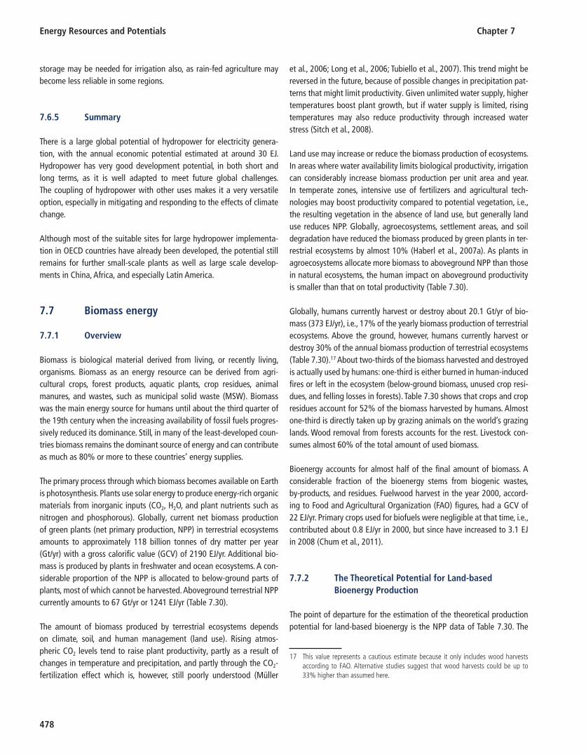
Energy Resources and Potentials Chapter 7
478
storage may be needed for irrigation also, as rain-fed agriculture may become less reliable in some regions.
7.6.5 Summary
There is a large global potential of hydropower for electricity genera-tion, with the annual economic potential estimated at around 30 EJ. Hydropower has very good development potential, in both short and long terms, as it is well adapted to meet future global challenges. The coupling of hydropower with other uses makes it a very versatile option, especially in mitigating and responding to the effects of climate change.
Although most of the suitable sites for large hydropower implementa-tion in OECD countries have already been developed, the potential still remains for further small-scale plants as well as large scale develop-ments in China, Africa, and especially Latin America.
7.7 Biomass energy
7.7.1 Overview
Biomass is biological material derived from living, or recently living, organisms. Biomass as an energy resource can be derived from agri-cultural crops, forest products, aquatic plants, crop residues, animal manures, and wastes, such as municipal solid waste (MSW). Biomass was the main energy source for humans until about the third quarter of the 19th century when the increasing availability of fossil fuels progres-sively reduced its dominance. Still, in many of the least-developed coun-tries biomass remains the dominant source of energy and can contribute as much as 80% or more to these countries’ energy supplies.
The primary process through which biomass becomes available on Earth is photosynthesis. Plants use solar energy to produce energy-rich organic materials from inorganic inputs (CO 2 , H 2 O, and plant nutrients such as nitrogen and phosphorous). Globally, current net biomass production of green plants (net primary production, NPP) in terrestrial ecosystems amounts to approximately 118 billion tonnes of dry matter per year (Gt/yr) with a gross calorific value (GCV) of 2190 EJ/yr. Additional bio-mass is produced by plants in freshwater and ocean ecosystems. A con-siderable proportion of the NPP is allocated to below-ground parts of plants, most of which cannot be harvested. Aboveground terrestrial NPP currently amounts to 67 Gt/yr or 1241 EJ/yr ( Table 7.30 ).
The amount of biomass produced by terrestrial ecosystems depends on climate, soil, and human management (land use). Rising atmos-pheric CO 2 levels tend to raise plant productivity, partly as a result of changes in temperature and precipitation, and partly through the CO 2 -fertilization effect which is, however, still poorly understood (M ü ller
et al., 2006 ; Long et al., 2006 ; Tubiello et al., 2007 ). This trend might be reversed in the future, because of possible changes in precipitation pat-terns that might limit productivity. Given unlimited water supply, higher temperatures boost plant growth, but if water supply is limited, rising temperatures may also reduce productivity through increased water stress (Sitch et al., 2008 ).
Land use may increase or reduce the biomass production of ecosystems. In areas where water availability limits biological productivity, irrigation can considerably increase biomass production per unit area and year. In temperate zones, intensive use of fertilizers and agricultural tech-nologies may boost productivity compared to potential vegetation, i.e., the resulting vegetation in the absence of land use, but generally land use reduces NPP. Globally, agroecosystems, settlement areas, and soil degradation have reduced the biomass produced by green plants in ter-restrial ecosystems by almost 10% (Haberl et al., 2007a ). As plants in agroecosystems allocate more biomass to aboveground NPP than those in natural ecosystems, the human impact on aboveground productivity is smaller than that on total productivity ( Table 7.30 ).
Globally, humans currently harvest or destroy about 20.1 Gt/yr of bio-mass (373 EJ/yr), i.e., 17% of the yearly biomass production of terrestrial ecosystems. Above the ground, however, humans currently harvest or destroy 30% of the annual biomass production of terrestrial ecosystems ( Table 7.30 ). 17 About two-thirds of the biomass harvested and destroyed is actually used by humans: one-third is either burned in human-induced fires or left in the ecosystem (below-ground biomass, unused crop resi-dues, and felling losses in forests). Table 7.30 shows that crops and crop residues account for 52% of the biomass harvested by humans. Almost one-third is directly taken up by grazing animals on the world’s grazing lands. Wood removal from forests accounts for the rest. Livestock con-sumes almost 60% of the total amount of used biomass.
Bioenergy accounts for almost half of the final amount of biomass. A considerable fraction of the bioenergy stems from biogenic wastes, by-products, and residues. Fuelwood harvest in the year 2000, accord-ing to Food and Agricultural Organization (FAO) figures, had a GCV of 22 EJ/yr. Primary crops used for biofuels were negligible at that time, i.e., contributed about 0.8 EJ/yr in 2000, but since have increased to 3.1 EJ in 2008 (Chum et al., 2011 ).
7.7.2 The Theoretical Potential for Land-based Bioenergy Production
The point of departure for the estimation of the theoretical production potential for land-based bioenergy is the NPP data of Table 7.30 . The
17 This value represents a cautious estimate because it only includes wood harvests according to FAO. Alternative studies suggest that wood harvests could be up to 33% higher than assumed here.

Tabl
e 7.
30 |
Glo
bal y
early
bio
mas
s fl o
ws
arou
nd th
e ye
ar 2
000.
USA
CAN
WEU
EEU
FSU
NA
FEA
FW
CASA
FM
EECH
NO
EAIN
DO
SAJP
NO
CNPA
SLA
CW
orld
[EJ/
yr]
Tota
l pot
entia
l NPP
b 15
7.4
138.
787
.326
.133
1.6
41.5
73.0
243.
115
0.2
16.9
129.
740
.164
.019
.48.
812
1.3
165.
760
8.9
2423
.7
Abov
egr.
pote
ntia
l N
PP b
85.7
76.4
48.9
15.3
179.
720
.839
.813
3.0
79.5
6.4
70.1
21.2
34.1
9.5
5.1
60.0
92.0
331.
413
09.0
Tota
l cur
rent
NPP
140.
913
2.0
79.5
20.2
298.
936
.059
.121
7.7
136.
315
.212
3.0
35.4
50.6
19.8
8.1
114.
114
0.6
563.
621
91.0
Abov
egro
und
curr
ent
NPP
85.1
73.4
50.8
13.6
165.
119
.732
.812
0.8
73.2
7.5
76.0
19.2
34.8
12.2
5.0
58.3
80.9
312.
512
41.0
Harv
este
d bi
omas
s 25
.7
4.6
20.4
5.
2 10
.4
5.3
6.9
10.9
6.
4 2.
6 29
.2
3.3
24.3
8.
2 1.
0 6.
2 13
.3
40.4
22
4.6
Harv
este
d pr
imar
y cr
ops
10.2
1.3
7.7
2.2
4.5
1.0
0.6
1.9
0.9
0.8
10.0
0.9
6.2
1.7
0.4
1.9
4.2
7.0
63.5
Harv
este
d cr
op
resi
dues
5.8
0.8
3.9
1.7
2.8
1.0
0.9
2.9
1.4
0.8
9.2
0.8
7.5
2.1
0.2
0.6
4.2
7.5
54.3
Biom
ass
graz
ed4.
80.
66.
00.
41.
32.
73.
53.
02.
71.
07.
11.
07.
13.
40.
23.
31.
721
.171
.0
Woo
d re
mov
als
(FAO
)4.
91.
92.
80.
91.
80.
52.
03.
11.
30.
02.
90.
63.
41.
00.
20.
53.
14.
935
.9
Biom
ass
dest
roye
d 9.
8 1.
8 7.
1 2.
5 8.
1 7.
5 5.
7 21
.4
14.2
0.
7 14
.1
3.4
10.9
2.
4 0.
4 3.
9 10
.6
23.5
14
8.0
Hum
an-in
duce
d fi r
es0.
30.
00.
30.
23.
66.
34.
317
.712
.50.
00.
92.
12.
30.
50.
02.
64.
514
.772
.8
Belo
wgr
ound
bio
mas
s4.
71.
13.
21.
12.
20.
40.
81.
90.
90.
35.
30.
63.
90.
90.
20.
62.
84.
435
.5
Unu
sed
crop
land
re
sidu
es3.
90.
53.
21.
01.
90.
70.
30.
80.
40.
35.
90.
33.
00.
70.
20.
71.
42.
427
.7
Felli
ng lo
sses
in
fore
sts
0.8
0.2
0.4
0.2
0.5
0.1
0.2
0.9
0.4
0.0
2.0
0.3
1.7
0.3
0.0
0.1
1.9
1.9
12.1
Use
of h
arve
sted
bi
omas
s 23
.8
3.3
21.0
5.
0 9.
4 5.
8 6.
9 10
.5
6.3
3.3
29.5
3.
2 23
.6
8.2
2.4
5.5
12.5
38
.6
219.
1
Plan
t-ba
sed
food
1.4
0.1
2.1
0.5
1.2
0.9
0.5
1.3
0.6
0.8
6.3
0.6
4.5
1.4
0.5
0.1
2.6
2.3
27.8
Feed
(gra
zing
, re
sidu
es)
12.2
1.6
12.8
2.2
4.9
4.0
4.3
4.7
3.9
2.0
14.7
1.5
15.4
5.2
1.0
4.8
4.1
29.8
129.
2
Woo
d5.
21.
03.
20.
81.
20.
62.
03.
11.
30.
13.
50.
63.
51.
00.
80.
33.
04.
836
.0
Oth
er u
ses
4.9
0.6
2.9
1.5
2.1
0.4
0.1
1.5
0.5
0.3
5.1
0.4
0.1
0.6
0.1
0.3
2.9
1.7
26.1
Fina
l bio
mas
s us
e 8.
7 1.
1 9.
0 1.
6 2.
4 1.
8 1.
8 6.
1 3.
0 1.
0 18
.5
1.9
11.4
3.
5 1.
8 0.
7 7.
3 7.
9 89
.5
Food
for h
uman
s2.
30.
23.
20.
81.
61.
00.
51.
40.
70.
87.
70.
64.
81.
50.
60.
22.
83.
033
.8
Tim
ber a
nd p
aper
3.3
0.4
2.9
0.4
0.4
0.1
0.1
0.2
0.2
0.1
1.4
0.1
0.2
0.1
0.9
0.2
0.7
0.9
12.4
Bioe
nerg
y (IE
A)2.
60.
52.
30.
40.
30.
61.
24.
42.
10.
08.
91.
16.
21.
80.
20.
23.
63.
440
.2
Oth
er u
ses
0.5
0.0
0.6
0.1
0.1
0.1
0.0
0.1
0.0
0.1
0.4
0.0
0.2
0.1
0.1
0.0
0.2
0.6
3.2
a G
ross
cal
orifi
c va
lue.
1 t
dry
mat
ter b
iom
ass
= 0
.5 t
carb
on =
18.
5 G
J.
b N
PP o
f the
veg
etat
ion
assu
med
to e
xist
in th
e ab
senc
e of
hum
an la
nd u
se u
nder
cur
rent
clim
ate
cond
ition
s.
Sour
ces:
Habe
rl et
al.,
2007
a ; IE
A, 2
007a
, 200
7b , 2
008b
; Kra
usm
ann
et a
l., 20
08 ; L
auk
and
Erb,
200
9 . a
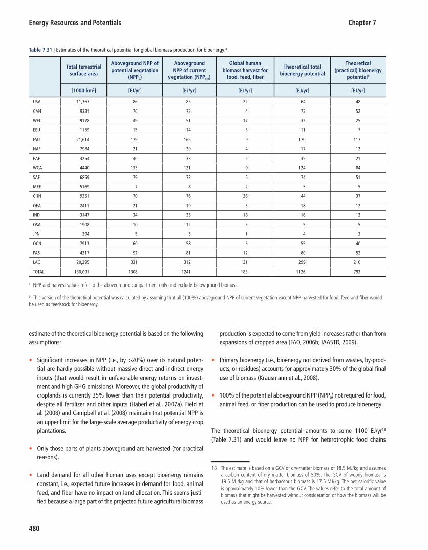
Energy Resources and Potentials Chapter 7
480
estimate of the theoretical bioenergy potential is based on the following assumptions:
Significant increases in NPP (i.e., by >20%) over its natural poten- •tial are hardly possible without massive direct and indirect energy inputs (that would result in unfavorable energy returns on invest-ment and high GHG emissions). Moreover, the global productivity of croplands is currently 35% lower than their potential productivity, despite all fertilizer and other inputs (Haberl et al., 2007a ). Field et al. ( 2008 ) and Campbell et al. ( 2008 ) maintain that potential NPP is an upper limit for the large-scale average productivity of energy crop plantations.
Only those parts of plants aboveground are harvested (for practical •reasons).
Land demand for all other human uses except bioenergy remains •constant, i.e., expected future increases in demand for food, animal feed, and fiber have no impact on land allocation. This seems justi-fied because a large part of the projected future agricultural biomass
production is expected to come from yield increases rather than from expansions of cropped area (FAO, 2006b ; IAASTD, 2009 ).
Primary bioenergy (i.e., bioenergy not derived from wastes, by-prod- •ucts, or residues) accounts for approximately 30% of the global final use of biomass (Krausmann et al., 2008 ).
100% of the potential aboveground NPP (NPP • 0 ) not required for food, animal feed, or fiber production can be used to produce bioenergy.
The theoretical bioenergy potential amounts to some 1100 EJ/yr 18 ( Table 7.31 ) and would leave no NPP for heterotrophic food chains
18 The estimate is based on a GCV of dry-matter biomass of 18.5 MJ/kg and assumes a carbon content of dry matter biomass of 50%. The GCV of woody biomass is 19.5 MJ/kg and that of herbaceous biomass is 17.5 MJ/kg. The net calorifi c value is approximately 10% lower than the GCV. The values refer to the total amount of biomass that might be harvested without consideration of how the biomass will be used as an energy source.
Table 7.31 | Estimates of the theoretical potential for global biomass production for bioenergy. a
Total terrestrial surface area
Aboveground NPP of potential vegetation
(NPP 0 )
Aboveground NPP of current
vegetation (NPP act )
Global human biomass harvest for
food, feed, fiber
Theoretical total bioenergy potential
Theoretical (practical) bioenergy
potential b
[1000 km 2 ] [EJ/yr] [EJ/yr] [EJ/yr] [EJ/yr] [EJ/yr]
USA 11,367 86 85 22 64 48
CAN 9331 76 73 4 73 52
WEU 9178 49 51 17 32 25
EEU 1159 15 14 5 11 7
FSU 21,614 179 165 9 170 117
NAF 7984 21 20 4 17 12
EAF 3254 40 33 5 35 21
WCA 4440 133 121 9 124 84
SAF 6859 79 73 5 74 51
MEE 5169 7 8 2 5 5
CHN 9351 70 76 26 44 37
OEA 2411 21 19 3 18 12
IND 3147 34 35 18 16 12
OSA 1908 10 12 5 5 5
JPN 394 5 5 1 4 3
OCN 7913 60 58 5 55 40
PAS 4317 92 81 12 80 52
LAC 20,295 331 312 31 299 210
TOTAL 130,091 1308 1241 183 1126 793
a NPP and harvest values refer to the aboveground compartment only and exclude belowground biomass.
b This version of the theoretical potential was calculated by assuming that all (100%) aboveground NPP of current vegetation except NPP harvested for food, feed and fi ber would be used as feedstock for bioenergy.
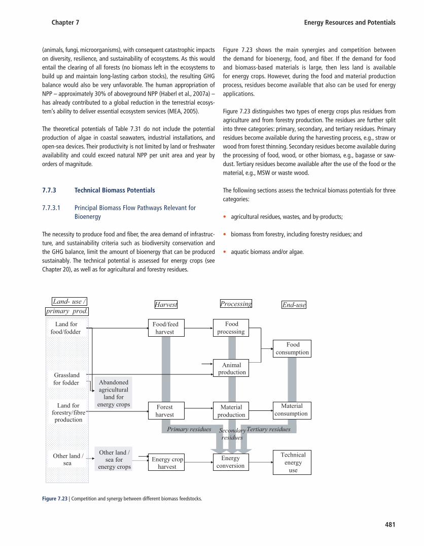
Chapter 7 Energy Resources and Potentials
481
(animals, fungi, microorganisms), with consequent catastrophic impacts on diversity, resilience, and sustainability of ecosystems. As this would entail the clearing of all forests (no biomass left in the ecosystems to build up and maintain long-lasting carbon stocks), the resulting GHG balance would also be very unfavorable. The human appropriation of NPP – approximately 30% of aboveground NPP (Haberl et al., 2007a ) – has already contributed to a global reduction in the terrestrial ecosys-tem’s ability to deliver essential ecosystem services (MEA, 2005 ).
The theoretical potentials of Table 7.31 do not include the potential production of algae in coastal seawaters, industrial installations, and open-sea devices. Their productivity is not limited by land or freshwater availability and could exceed natural NPP per unit area and year by orders of magnitude.
7.7.3 Technical Biomass Potentials
7.7.3.1 Principal Biomass Flow Pathways Relevant for Bioenergy
The necessity to produce food and fiber, the area demand of infrastruc-ture, and sustainability criteria such as biodiversity conservation and the GHG balance, limit the amount of bioenergy that can be produced sustainably. The technical potential is assessed for energy crops (see Chapter 20), as well as for agricultural and forestry residues.
Figure 7.23 shows the main synergies and competition between the demand for bioenergy, food, and fiber. If the demand for food and biomass-based materials is large, then less land is available for energy crops. However, during the food and material production process, residues become available that also can be used for energy applications.
Figure 7.23 distinguishes two types of energy crops plus residues from agriculture and from forestry production. The residues are further split into three categories: primary, secondary, and tertiary residues. Primary residues become available during the harvesting process, e.g., straw or wood from forest thinning. Secondary residues become available during the processing of food, wood, or other biomass, e.g., bagasse or saw-dust. Tertiary residues become available after the use of the food or the material, e.g., MSW or waste wood.
The following sections assess the technical biomass potentials for three categories:
agricultural residues, wastes, and by-products; •
biomass from forestry, including forestry residues; and •
aquatic biomass and/or algae. •
Other land / sea for
energy crops
Land for forestry/fibre production
Energy crop harvest
Food/feedharvest
Forestharvest
Energyconversion
Foodprocessing
Technicalenergy
use
Foodconsumption
Materialproduction
Materialconsumption
Primary residues Tertiary residuesSecondary residues
Animal production
Land forfood/fodder
Abandonedagricultural
land for energy crops
Other land / sea
Grasslandfor fodder
Land- use /primary prod.
Harvest Processing End-use
Figure 7.23 | Competition and synergy between different biomass feedstocks.

Energy Resources and Potentials Chapter 7
482
The energy potential from energy crops on cropland, abandoned agricul-tural land, or grazing land is discussed in Chapter 20 .
7.7.3.2 Crop Residues, Municipal Solid Wastes, and Animal Manures
Overview Large quantities of organic residues and wastes are produced annually, including crop residues, animal manures, and MSW. Rational utilization of these can produce energy, normally cost-effectively, and minimize environmental impacts that are often caused by other management and/or disposal methods.
Crop residues Two types of residues are associated with crop production. These are pri-mary, i.e., harvest or field residues, and secondary, i.e., processing resi-dues. The recoverable fraction (RF) of a residue depends on the amount that could be collected practically and, in the case of field residues, on the amount that should be left in the field for maintaining soil quality.
Annual crop production in 2005 was estimated from the FAO online database (FAO, 2009 ). Values of residue to product ratio (RPR) for dif-ferent crops are taken from the open literature (Fischer et al., 2007 ; Koopmans and Koppejan, 1998 ; Bhattacharya, 1991 ). The RPR values for primary residues of cereal crops depend on the level of technology used for cereal production. Higher levels of technology, including irriga-tion and fertilization, result in higher yields per hectare and lower values of RPR; RPR values selected in this study for 2050 correspond to higher levels of technology (Fischer et al., 2007 ). For the year 2005, region-spe-cific RPR values were selected and assumed based on literature reviews; values corresponding to the average of higher and lower levels of tech-nology are assumed for the regions for which no RPR values could be found in the literature.
Residue generation from cereal crop production for the year 2050 was estimated using projected production growth rates of cereals in developing, industrial, and transition countries from FAO ( 2006a ). For estimating residue generation from the other crops, their production growth rates in different country categories are assumed to be the same as the projected rates for all food and non-food commodities obtained from FAO ( 2006b ).
Table 7.32 shows the estimated energy potentials of crop residues in 2005 and 2050 for the 18 GEA regions. The total world technical poten-tial of crop residues in 2050 is estimated to be 49.4 EJ.
Assuming RF values for different crops in the range 0.5–0.75, Hakala et al. ( 2009 ) estimated the world technical potential of field residues in 2050 to be 38–41 EJ; adding the process residue potential of 16 EJ (Smeets et al., 2007 ), the total technical potential of crop residues would be 54–57 EJ. These estimates for 2050 may be compared with the range
10–32 EJ/yr derived by Hoogwijk ( 2004 ) and 46–66 EJ by Smeets et al. ( 2007 ).
Differences in crop-residue energy potential estimated by different authors mainly result from differences in their assumed RPR and RF values and crop-production projection methodologies.
Municipal solid wastes MSW consists of biogenic (i.e., renewable) and non-biogenic (i.e., non-renewable) constituents. The energy potential of the biogenic compo-nents was estimated from their energy values (US EIA, 2007 ), the total generation of MSW, assumed values for the recoverable fraction from MSW for energy, and the MSW composition. MSW composition and generation per capita for different countries/regions for the year 2000 were obtained from IPCC ( 2006 ); country/region-specific values were obtained, in some cases, from the literature.
MSW generation per capita is known to increase with growth in gross domestic product (GDP). Adhikari et al. ( 2006 ) established a relationship between MSW generation per capita and GDP per capita to project future MSW generation from expected growth in GDP per capita; this approach was used in this study. National GDP values were taken from World Bank ( 2008a ) and the projected future national and/or regional growth rates obtained from IEA ( 2006a ); population data for the years 2005 and 2050 were obtained from United Nations Population Division ( 2008 ).
Since an increase in MSW generation is not expected to continue indef-initely, Monni et al. ( 2006 ) projected a maximum future annual MSW generation of 900 kg/capita; this value was used in this assessment.
In this study, estimations for recycling of MSW organic matter through-out the world by 2050 are guided by a scenario for the EU-15 countries developed by Smith et al. ( 2001 ) for the year 2020: 60% paper recycling and 60% separation of food and yard-trimming wastes (two-thirds of the latter is assumed to be composted) and the remaining one-third used for anaerobic digestion. Thus, 60% of food and yard waste is avail-able for energy purposes.
In 2005, leather and rubber recycling in the United States was 14.3%, while recycling of textiles was 15.3%; 9.5% of wood in MSW in the United States was recycled. It is assumed that 15% of both leather and textiles would be recycled in 2050 in all countries; the amount of wood recycled is assumed at 10%.
The theoretical potential of MSW is assumed to be the energy potential of all MSW produced in a country without any recycling, while technical potential is assumed to be the same as the recoverable potential.
As shown in Table 7.32 , the total world recoverable potential of MSW in 2050 is estimated to be 11.02 EJ; this value can be compared with 1–3 EJ in 2050 as estimated by Hoogwijk ( 2004 ) and around 17 EJ as estimated by Smeets et al. ( 2007 ).

Tabl
e 7.
32 |
Ener
gy p
oten
tials
of c
rop
resi
dues
, MSW
, and
ani
mal
was
tes
in E
J/yr.
Regi
on
Crop
res
idue
sM
SWA
nim
al w
aste
s
2005
2050
2005
2050
2005
2050
Theo
reti
cal
Tech
nica
lTh
eore
tica
lTe
chni
cal
Theo
reti
cal
Tech
nica
lTh
eore
tica
lTe
chni
cal
Theo
reti
cal
Tech
nica
lTh
eore
tica
lTe
chni
cal
USA
7.54
2.68
9.32
3.28
2.16
0.92
3.19
1.33
3.19
1.7
5.67
3.03
CAN
1.32
0.55
2.18
0.6
0.27
0.14
0.3
0.12
0.5
0.27
0.88
0.47
WEU
5.55
2.2
6.39
2.56
2.05
0.86
3.38
1.28
3.34
1.74
5.94
3.09
EEU
2.5
0.91
1.75
0.66
0.43
0.18
0.56
0.21
0.56
0.31
10.
55
FSU
4.07
1.62
4.51
1.92
0.77
0.34
1.16
0.41
1.85
0.93
3.28
1.65
NAF
1.98
0.79
2.04
0.93
0.28
0.1
0.58
0.2
1.59
0.75
2.84
1.33
EAF
1.41
0.57
1.98
0.91
0.31
0.18
0.79
0.19
20.
943.
561.
67
WCA
4.15
1.58
5.29
2.22
0.57
0.16
1.49
0.55
1.83
0.85
3.25
1.51
SAF
1.88
1.05
3.41
1.63
0.32
0.08
0.9
0.27
1.32
0.64
2.34
1.14
MEE
1.28
0.54
2.15
0.95
0.39
0.18
1.11
0.46
0.78
0.36
1.38
0.64
CHN
12.0
86.
2514
.87
7.81
2.09
0.59
4.41
1.54
5.6
2.8
9.96
4.99
OEA
1.36
0.55
1.55
0.66
0.24
0.05
0.39
0.13
0.56
0.26
10.
46
IND
9.31
4.08
14.1
56.
750.
960.
152.
580.
777.
083.
4712
.59
6.17
OSA
3.04
1.27
4.25
1.95
0.5
0.09
1.09
0.33
1.66
0.82
2.95
1.46
JPN
0.34
0.14
0.33
0.14
0.56
0.19
0.87
0.31
0.17
0.1
0.29
0.17
PAS
7.29
3.18
9.49
4.52
0.93
0.32
2.63
1.09
1.46
0.76
2.6
1.35
OCN
1.52
0.66
1.47
0.67
0.16
0.09
0.2
0.08
1.32
0.59
2.34
1.65
LAC
11.4
15.
6921
.64
11.2
81.
440.
783.
991.
758.
874.
4415
.79
7.9
WO
RLD
78.0
334
.32
106.
7849
.45
13.1
55.
429
.63
11.0
243
.66
21.7
177
.68
39.2
1
The
ener
gy p
oten
tials
of h
arve
st o
r fi e
ld re
sidu
es a
nd p
roce
ssin
g re
sidu
es w
ere
estim
ated
as
follo
ws:
Resi
due
ener
gy p
oten
tial (
EJ/y
r) =
bon
e dr
y re
sidu
e pr
oduc
tion
(Mt/y
r) ×
reco
vera
ble
fract
ion
of re
sidu
e pr
oduc
tion
× g
ross
hea
ting
valu
e of
bon
e-dr
y re
sidu
e (E
J/Mt).
Bone
dry
resi
due
prod
uctio
n (M
t/yr)
= d
ry m
atte
r of c
rops
pro
duce
d (M
t/yr)
× re
sidu
e to
pro
duct
(or c
rop)
ratio
on
dry
basi
s.
Incl
udes
resi
due
ener
gy p
oten
tials
of t
he fo
llow
ing
crop
s:
Cere
als:
whe
at, r
ice,
bar
ley,
mai
ze, r
ye, o
ats,
mill
ets,
sorg
hum
.
Suga
r cro
ps: s
ugar
bee
t, su
gar c
ane.
Puls
es: p
eas,
chic
k pe
as, c
ow p
eas,
pige
on p
eas,
bean
s, br
oad
bean
s, le
ntils
, pul
ses
of m
inor
rele
vanc
e.
Oil
crop
s: gr
ound
nuts
, rap
esee
d, s
oybe
ans,
sunfl
ow
er s
eed,
saf
fl ow
er s
eeds
, lin
seed
, ses
ame
seed
, cas
tor b
ean,
oth
er o
ilsee
ds o
f min
or re
leva
nce.
Tree
nut
s: al
mon
ds, b
razi
l nut
s, ca
shew
nut
s, ch
estn
uts,
haze
l nut
s, ko
la n
uts,
pist
achi
os, w
alnu
ts.
Frui
ts: a
pple
s, ap
ricot
s, av
ocad
os, b
anan
as, c
ashe
w a
pple
s, ch
errie
s, ci
trus
frui
t, da
tes,
fi gs,
fruit
grap
efru
it (in
clud
ing
pom
elos
), gr
apes
, kiw
i fru
it, le
mon
s an
d lim
es,
man
goes
, man
gost
eens
, gua
vas,
oran
ges,
papa
yas,
peac
hes
and
nect
arin
es, p
ears
, per
sim
ons,
pine
appl
es, p
lant
ains
, plu
ms
and
sloe
s, qu
ince
s, ra
spbe
rrie
s, so
ur c
herr
ies,
ston
e fru
it, ta
nger
ines
, man
darin
s an
d cl
emen
tines
.
Tube
r cro
ps: c
assa
va, p
otat
oes,
swee
t pot
atoe
s, ya
ms.
Oth
er c
rops
: cof
fee,
cot
ton,
jute
.
Not
es:
The
ener
gy p
oten
tial o
f man
ure
gene
rate
d an
nual
ly b
y an
imal
type
i is
es
timat
ed a
s fo
llow
s:
Tota
l vol
atile
sol
id p
rodu
ced
annu
ally
by
an a
nim
al o
f a g
iven
type
i ,
VS i (
kg/y
r) =
365
× a
nim
al p
opul
atio
n (h
ead)
× a
vera
ge v
olat
ile s
olid
s pr
oduc
tion
per h
ead
for a
nim
al o
f typ
e i p
er d
ay (k
g vo
latil
e so
lid/h
ead/
day)
.
Tota
l dry
man
ure
prod
uced
ann
ually
by
an a
nim
al o
f a g
iven
type
i ,
TS i (
kg/y
r) =
VS i /
vola
tile
fract
ion
Tota
l ann
ual e
nerg
y po
tent
ial =
TS i
× h
eatin
g va
lue
of m
anur
e on
dry
ba
sis.

Energy Resources and Potentials Chapter 7
484
Animal manures The number of animals in 2005 was obtained from the FAO database on live animals (FAO, 2009 ). The number of all animals was assumed to increase at rates corresponding to the projected annual growth in world livestock production (FAO, 2006c ) – these are 1.6% during the period up to 2030 and 0.9% in 2030–2050. Values of kilogram of vola-tile solid/head/day were obtained from the IPCC ( 2006 ); the amounts of total dry solids produced were estimated from these, assuming suit-able values of volatile fraction. Values of RFs of manures were obtained from TERI ( 1985 ) and NRCS (1995). Based on literature reviews, the heating values of dry animal manures were assumed to be 17 MJ/kg for swine: 12.9 MJ/kg chicken, and 16 MJ/kg for other animals.
As shown in Table 7.32 , the energy potential of recoverable manures was estimated to be 39.2 EJ in 2050. Johansson et al. ( 1993 ) estimated the heating value of annual recoverable manures in 2050 to be 25 EJ. Based on a literature review, Hoogwijk ( 2004 ) estimated the recover-able potential of animal manures to be 9–25 EJ.
Differences in the energy potential of animal manures reported by different authors appear to result mainly from differences in pro-jected manure-generation values and assumed RFs, as well as heating values.
Technical potential of forestry residues Figure 7.23 distinguishes three categories of forestry residues: primary (available from additional fellings or as residues from thinning or final fellings), secondary (available when processing the forest products, e.g., sawdust), and residues (available after end use, i.e., waste wood).
Various studies have assessed the future potential for forestry resi-dues (e.g., Berndes et al., 2003 ; Smeets and Faaij, 2007 ; IPCC, 2007 ;
Anttila et al., 2009). The Anttila et al. (2009) study estimates a pri-mary forestry residue potential ranging from 5 EJ/yr to 9 EJ/yr globally, including logging residues from present cuttings, the stemwood from supplementary cutting, and the logging residues from supplementary cutting. This range is low compared to other estimates for the year 2050, e.g., 28 EJ/yr (Smeets et al., 2007 ) or 12–74 EJ/yr (IPCC, 2007 ). The difference largely results from the inclusion or not of secondary and tertiary residues. Secondary and tertiary residues can be 3–5 times higher than the primary residues Smeets et al. ( 2007 ). To estimate the regional potential for all forestry residues, the data from Anttila et al. (2009) were increased by a factor of four to include the other residues (see Table 7.33 ).
7.7.3.3 Aquatic Biomass Land use constraints, competition with food, and demand for biomass with high caloric value have made marine-based biomass an attractive alternative supply option over past years. However, land-based biomass systems are far more developed than sea-based systems whose eco-nomic viability has yet to be determined. In addition, estimates of algae energy potentials are scarce and quite uncertain, as most are extrapola-tions from small-scale (pilot) projects.
Aquatic biomass can be grouped into three categories: microalgae, sea-weed, and sea grass. The production of aquatic biomass depends on various factors, such as irradiation, limpidity, temperature, sea condi-tions, and nutrients. Naturally, regional variations can be significant. Promising concepts for aquatic biomass include (1) land-based open ponds for microalgae, (2) horizontal lines between offshore infrastruc-ture, e.g., wind farms for macroalgae (seaweed), (3) vertical lines near shore in densely used areas and nutrient-rich areas for macroalgae, and (4) macroalgae colonies at open sea up to 2000 km offshore (Florentinus et al., 2008 ). The total potential at a global scale is assessed at over
Table 7.33 | Estimate of technical potential of forestry residues in comparison with the forestry residue estimates from IPCC ( 2007 ), Anttila et al. (2009) , and Smeets et al. ( 2007 ). Anttila et al. (2009) only includes primary residues.
Technical potential IPCC AR4 Anttila et al. (2009) Smeets et al. ( 2007 )
Regions Low High Low High Low HighWood
harvestAll forestry
residues
[EJ]
North America 5.8 11.9 3 11 1.5 3 2 10
OECD Europe 3.8 6.7 1 4 1 1.7 1 5
Japan + Australia + NZ 1.1 1.8 1 3 0.4 0.7 0 2
FSU + Eastern Europe 3 5.4 2 10 0.8 1.3 1 3
Latin America 1.6 3.8 1 21 0.4 0.9 1 3
Africa 0.6 1.4 1 10 0.1 0.3 0 0
Centrally planned Asia 2 3 1 5 0.5 0.7 2 6
Other Asia 0.7 1.3 1 8 0.1 0.1 1 1
Middle East 0 0.1 1 2 0 0 0 0
World 18.8 35.1 12 74 4.7 8.7 8 30

Chapter 7 Energy Resources and Potentials
485
6000 EJ/yr. For the first three production categories the potential is 235 EJ/yr. Algae production at open sea has by far the largest potential, but is also the most complicated.
7.7.4 Summary of Global Technical Bioenergy Potential Estimates
Table 7.34 summarizes the various bioenergy supply potentials. The total global technical bioenergy potential for the year 2050 varies between 162–267 EJ/yr – a range considerably lower than previous analyses, which suggested global bioenergy potentials around 400 EJ/yr by 2050. This lower estimate largely results from lower expectations about the overall potential to grow dedicated bioenergy crops. In general, these potentials are highly uncertain. However, it is increasingly recognized that land demand for food production and feed supply, urban and infra-structure areas, biodiversity conservation, and the need to maintain a favorable GHG emission balance (i.e., no deforestation) pose definite limits on land availability for bioenergy production. Moreover, new studies suggest that the productive potential of land areas available for bioenergy is much lower than previously thought (Johnston et al., 2009).
7.7.5 Economics of Bioenergy Production and Supply Cost Curves
7.7.5.1 Supply Cost curves of Bioenergy Crops
Costs for energy crops include capital costs for equipment and infra-structures, plant and seed material, land rent, labor costs, energy (e.g., for drying and transport), material expenditures (e.g., fertilizer and water), and storage. Bottom-up studies indicate that costs for drying
and storage are the least certain and therefore are often excluded (de Wit and Faaij, 2010). Future production costs will depend on productivity developments, labor costs, land rental, and experience. Lignocellulosic energy crops have the lowest cost of all energy crops because of the low input requirements and relative high productivities. Costs in Europe range from 1.5–4.5 € /GJ, 19 while other crops, such as starch, sugar, and oil crops, cost between 5–15 € /GJ (de Wit and Faaij, 2010). Similar results are found for the United Kingdom (E4Tech, 2009 ), where costs for energy crops in 2030 are generally estimated at 2.0–3.5 £/GJ. The cost curves for Europe and the United Kingdom as reported by de Wit and Faaij (2010) and E4Tech ( 2009 ) are all relatively flat in the longer term. In the EU about 90% of lignocellulosic crops are available at costs between 1.5–3 € /GJ by 2030, with the remaining amount between 3–6 € /GJ (de Wit and Faaij, 2010). For the United States projected costs for delivered biomass in 2025 are very low for forest residues (US 2005 $1.0–2.0/GJ) for limited amount (up to 1.5 EJ/yr). For larger sup-plies (up to 7 EJ/yr) energy crops have costs around US 2005 $3.5–4.0/GJ (Chum et al, 2011 ).
Projected costs for energy crops include capital costs for equipment and infrastructures, plant and seed material, land rent, labor costs, energy (e.g., for drying and transport to conversion facilities), material expenditures (e.g., fertilizer and water), and storage. Bottom-up stud-ies indicate that costs for drying and storage are the least certain and therefore are often excluded (de Wit and Faaij, 2010). Future produc-tion costs will depend on productivity developments, labor costs, land rental, and experience. Lignocellulosic energy crops have the lowest cost of all energy crops because of the low input requirements and relative high productivities. Estimated costs in Europe range from 1.5–4.5 € /GJ and a production volume of about 7 EJ/yr, while other crops, such as starch (3 EJ/yr), sugar (6 EJ/yr), and oil crops (3 EJ/yr), cost between 5–15 € /GJ (de Wit and Faaij, 2010). Similar results are found for the United Kingdom (E4Tech, 2009 ), where costs for energy crops in 2030 are generally estimated at 2.0–3.5 £/GJ. The lignocel-lulosic cost curves for Europe and the United Kingdom as reported by de Wit and Faaij (2010) and E4Tech ( 2009 ) are all relatively flat in the longer term. In the EU about 90% of lignocellulosic crops are avail-able at costs between 1.5–3 € /GJ by 2030, with the remaining amount between 3–6 € /GJ (de Wit and Faaij, 2010).
Long-term global economic supply potentials for dedicated energy crops were assessed by Hoogwijk et al. ( 2009 ). This study analyzed four distinct land-use scenarios using a production function approach with costs for labor, capital, land, and transport to the main distribu-tion centers. Regional differences reflect differences in productivity, labor, and land costs. The bioenergy production cost ranges shown in Figure 7.24 are based on the production cost distribution of that land-use scenario with its cost distribution representing the middle of all the scenario distributions and applied to the technical potentials
Table 7.34 | Summary of global technical bioenergy supply potentials in 2050.
ResourceMIN MAX
Comments[EJ] [EJ]
Dedicated bioenergy crops
44 133 High uncertainty, depends on yields, diets, technology, and climate change
Crop residues 49 Soil conservation issues need to be addressed; GHG balance might depend on soil carbon balance (currently poorly understood)
Manures 39 Relatively small uncertainty and few, if any, environmental issues
Municipal solid waste 11 Relatively small uncertainty and few environmental issues
Forestry 19 35 Competition for other uses may reduce availability of residues
Total, excluding aquatic
162 267 19 Note that the market for lignocellulosic crops in particular is still small and costs in
many literature sources are based on desktop data.

Energy Resources and Potentials Chapter 7
486
summarized in Table 7.35 . (The ranges are lower than those reported in the aforementioned studies.)
Figure 7.24 shows the aggregate global biomass supply cost curve based on the ‘mean’ regional supply volumes and the production-cost distribution data of Table 7.35 .
7.7.5.2 Supply Cost Curves of Agricultural Residues and Municipal Solid Waste
In general, the cost of biomass residues is site-specific. Approximate val-ues of residue costs are assumed for the purpose of this study. Based on Haq and Easterly ( 2006 ), the following cost values, including transporta-tion and payment for a farmer premium, are assumed to be valid for the United States and all other developed countries and regions for the year 2005: 46 $/t for corn stover, wheat straw, and field residues of sorghum, barley, oats, rye, and cotton field trash, and 41 $/t for rice straw and processing residues. The cost of all other crop residues is assumed to be 46 $/t.
Based on Purohit et al. (2002), the cost of residues in India in 2005, including transportation, is estimated to be 25 $/t. The average cost of cellulosic biomass, including transportation, is assumed to be 22 $/t in China (Yang et al., 2005 ). The estimated cost of field residues in Nigeria has been reported as 23.1 $/t (Jekayinfa and Scholz, 2007 ). Based on the cost values of India, China, and Nigeria, the average cost of all agri-cultural crops in all developing countries, except India and China, in the year 2005 has been assumed to be 23.5 $/t.
The farm-gate cost of residues in United States mostly reflects the cost of their collection, i.e., delivering them in bales at the edge of the field. It has been projected that improvements in collection technology will significantly reduce the collection cost of residues below the 2005 level (Walsh, 2008 ). Farmer premiums, however, are likely to increase in the future. Based on the above considerations, it is estimated that the cost of residues in 2050 will remain at the 2005 level for all developed countries.
In developing countries, residues collection in 2050 is assumed to be based on machines similar to those used in developed countries; con-sidering that the cost of labor involved in collection and transportation would remain lower in developing countries, the costs of residues in these countries in 2050 is assumed to be 80% of the estimated costs for developed countries.
MSW may have negative costs because of tipping fees. The average fee per tonne in the United States was $33.74 in 2002 and $34.29 in 2004 (Repa, 2005 ); the tipping fee was assumed to be 35 $/tonne in 2005. Based on the fees of six sites in Canada (Statistics Canada, 2005 ), the average fee for Canada is about 49 $/t. The following average 2005 tipping fees per tonne were assumed: Europe, $100; Japan, $150; OCN region, $32; China, $20 (based on the range 10–30 $/t, reported by Themelis and Themelis ( 2007 )); developing countries of Asia, $5; and Latin America, $15; while India and the remaining regions have no tip-ping fees.
The tipping fee to breakeven in case of plasma gasification of MSW in Canada has been estimated to be $35 (Young, 2006 ); the value is likely to be less in the future because of improvements in technology. For this
0
1
2
3
4
5
6
7
0 10 20 30 40 50 60 70 80 90
$/G
J
EJ/yr
Figure 7.24 | Bioenergy crops supply cost curve (average biomass supply of Table 7.35 ).
Table 7.35 | Technical and economic potential of energy crops.
Technical potential
Potential cost categories
Low [EJ]
High [EJ]
<1 $/GJ [%]
<2 $/GJ [%]
<4 $/GJ [%]
>4 $/GJ [%]
USA 1.6 3.3 0 57 80 20
CAN 2.73 9.87 0 77 85 15
WEU 1.7 4.85 0 44 94 6
EEU 0.69 2.74 0 89 89 11
FSU 3.09 8.61 0 77 79 21
NAF 0.72 2.6 0 50 50 50
EAF 0.34 0.4 20 40 40 60
WCA 11 34.34 17 67 83 17
SAF 0.06 1.12 0 0 0 100
MEE 0.61 1.52 0 0 33 67
CHN 2.76 7.38 0 0 46 54
OEA 1.74 4.58 0 17 50 50
IND 0.12 0.65 0 17 50 50
OSA 1.45 7.11 0 17 50 50
JPN 3.09 6.89 0 44 94 6
OCN 4.12 18.06 20 80 83 17
PAS 5.64 10.91 20 80 83 17
LAC 2.23 7.74 0 27 68 32
TOTAL 43.69 132.67
Source: Adapted from Hoogwijk et al., 2009 .

Chapter 7 Energy Resources and Potentials
487
assessment, uniform tipping fees are US 2005 $40/t in 2050 and have been assumed for all countries and regions by 2050, while animal manures are assumed to be available at zero cost. The supply cost curve for agri-cultural residues and MSW is shown in Figure 7.25 .
7.7.5.3 Economic Potential of Bioenergy from Forestry
Forest residues are currently traded internationally, mostly in the form of wood pellets. The dominant raw material for wood-pellet produc-tion has traditionally been processing residues as sawdust. The prices of wood pellets for Europe range from 170–270 € /t (10–16 € /GJ) in a two-year period (UNECE/FAO, 2009 ) and for the Russian market from 95–165 € /t (6–10 € /GJ) (Junginger et al., 2009 ). The pellet market is integrated in the entire wood system and therefore influenced by the economic crisis, i.e., some wood-pellet producers have had problems with raw material supply (UNECE/FAO, 2009 ).
No global potential estimates include the production costs of forestry residues or pellets. Some assessments of the costs in Europe indicate levels ranging from 2.2–7.4 US 2000 $/GJ (Lindner et al., 2005 ). Extensive cost curves at a country level from (Asikainen et al., 2008 ) taking transport distance as the main varying parameter, result in compa-rable levels of around 2.5–7.5 € /GJ. For Denmark, costs have been assessed below 1 US 2000 $/GJ (Nord-Larson and Talbot, 2004 ). Estimates for Japan indicate costs in the order of 10–35 $/GJ (Yoshioka et al., 2006 ).
No studies include cost reductions caused by technological progress. Some cost curves for residues are known at the country level, e.g., for the United States (Walsh, 2008 ) and for some European countries (Asikainen et al., 2008 ). In general, costs are largely a function of trans-port distance, but a detailed breakdown is not provided. For the glo-bal potential it is assumed that 100% can be delivered at costs below 50 € /GJ and 10% at costs below 1 € /GJ.
7.7.5.4 Cost Estimates of Aquatic Biomass
The costs for algae cultivation are still high. Florentinus et al. ( 2008 ) estimate costs for biomass in the range of 300–700 € /t or even 1000 € /t of dry matter, or 18–60 € /GJ assuming a lower heating value of 16 GJ/t and significant technological improvements.
7.7.6 Social and Environmental Aspects of Bioenergy Use
Bioenergy is either produced by planting dedicated bioenergy crops or by using by-products, residues, and wastes from agriculture, forestry, food processing, and other economic activities (see Figure 7.23 ). These pathways can have environmental effects that are fundamentally differ-ent (Cherubini et al., 2009 ). The two pathways are therefore discussed in turn.
7.7.6.1 Environmental and Social Effects of Bioenergy Crop Plantations
Growing dedicated bioenergy crops can have positive and negative envi-ronmental and social impacts. For example, growing bioenergy crops increases the demand for agricultural products and creates income in the agricultural sector. However, demand for bioenergy crops may lead to rising agricultural prices (World Bank, 2008b ) and reduce affordable food supply, in particular for the poor.
Likewise, bioenergy can help to reduce GHG emissions, but when emis-sions from direct and indirect land-use changes (e.g., deforestation) are included, GHG emissions of bioenergy can be large, indeed even higher than those of fossil-fuel based alternatives (Searchinger et al., 2008 ; WBGU, 2008 ).
To establish how much bioenergy can be produced without harming the environment, and without adverse social and economic impacts undermining gains, requires a systems approach that takes into account the relevant interactions between various land uses and socioeconomic functions of biomass (food, fiber/materials, energy).
The environmental effects of bioenergy plantations are species-specific as well as site-specific. Perennial grasses such as switchgrass, miscant-hus, and short-rotation coppice are ecologically less demanding than food crops in terms of impacts on soils, soil erosion, biodiversity, nutrient leaching, pesticide application, etc. (Cherubini et al., 2009 ). Conversion of grasslands or forests for bioenergy production may cause dire eco-logical consequences. The environmental impacts of bioenergy depend only to some extent on the specific bioenergy plant and more on the previous use of the land on which it is planted (Gibbs et al., 2008 ).
Land demand is a central environmental issue associated with the expanding use of bioenergy crops (Sagar and Kartha, 2007 ; Firbank,
-4
-3
-2
-1
0
1
2
3
4
0 5 10 15 20 25 30 35 40 45 50 55 60 65 70 75 80 85 90 95
Prod
uc�
on c
osts
$/G
J
EJ
Current technoloy
2050 technology
Figure 7.25 | Aggregate supply cost curve 20 for MSW, animal wastes, and crop resi-dues. Negative costs are avoided tipping fees.
20 See footnote 7.

Energy Resources and Potentials Chapter 7
488
2008 ). Once considered a local environmental issue, it is increasingly recognized that land use has become a pervasive driver of global environmental change (Foley et al., 2005 ). The Millennium Ecosystem Assessment (MEA, 2005 ) concluded that land use has already reduced the ability of ecosystems to deliver vital ecosystem services. Large-scale bioenergy plantations would increase humanity’s pressures on global terrestrial ecosystems and contribute to biodiversity loss (Haberl et al., 2009 ).
Bioenergy plantations usually reduce the amount of carbon stored in ecosystems compared to undisturbed ecosystems (Schimel, 1995 ; Watson et al., 2000 ), while land conversion and biomass harvest can lead to loss of soil organic matter and significant net emissions (Pulleman et al., 2000 ; Lal, 2004 ; see also Chapter 20 ). In addition to the emissions from land use, GHG emissions also result from the energy required to produce bioenergy, and from the production and use of fertilizers, pesticides, and all other activities of the full process chain. Gibbs et al. ( 2008 ) concluded that the expansion of bioenergy into carbon-rich ecosystems (e.g., forests) leads to ‘carbon payback times’ of decades to centuries, whereas GHG avoidance is almost instantaneous if degraded or already cultivated land is used. For areas with lower embedded carbon such as grasslands or savannahs and for high yield biomass feedstocks payback periods can be less than a decade.
Water demand of bioenergy crops may cause environmental and social problems. Humans already use or regulate more than 40% of all freshwater resources globally (MEA, 2005 ). Global water demand grows by 10% per decade adding to water supply stress in many regions. Agriculture currently demands some 70% of all freshwater use (UNEP, 2009 ), of which 2% was used for bioethanol production (WBGU, 2008 ).
The production of bioenergy uses 70–400 times more water per unit of energy than other primary energy carriers, excluding hydropower, and ranges from 24–143 m 3 /GJ, with Jatropha having the largest water foot-print among 12 bioenergy crops analyzed in a recent study (Gerbens-Leenes et al., 2009 ). The amount of water per unit of energy is highly dependent on the crops used, the efficiency of the cropping system, and the local hydrological and soil conditions. On a positive note, bioenergy plantations in marginal areas may alleviate water-related problems, i.e., local water harvesting and run-off collection may reduce water-related erosion (Berndes, 2008 ).
Bioenergy produced on currently grazed lands can have large-scale impacts on livestock-rearing subsistence farmers. These may be posi-tive or negative, depending on the implementation strategy. Large-scale bioenergy plantations owned and operated by international, vertically integrated corporations tend not to benefit the local farming communi-ties as most of the revenue is generated in the production stage that involves sophisticated biochemical conversion technologies (Sagar and Kartha, 2007 ). However, small-scale locally owned and operated plants,
as well as sustainability certification systems, might help ensure that benefits accrue to the local farming communities (Lewandowski and Faaij, 2006 ).
7.7.6.2 Environmental and Social Implications of Using By-products, Residues, and Wastes
In contrast to bioenergy crops, bioenergy production from agricultural by-products, residues, and wastes does not (1) require additional land or land use changes, (2) compete with food or fiber production, (3) affect agricultural and food prices, and (4) require large amounts of additional scarce inputs such as freshwater (Berndes, 2008 ). On the contrary, using biomass residues may help alleviate energy shortages, reduce landfill requirements, and create employment opportunities. However, there may also be negative environmental effects, depend-ing on the respective biomass flow as well as on technology and management.
The agricultural residue straw can deliver substantial amounts of energy. However, straw plays a vital role for soil fertility, soil carbon pools, and the mitigation of water and wind erosion (Lal, 2005 , 2006 ; Wilhelm et al., 2007 ). WBGU ( 2008 ) assumes about half of all crop residues could be used to produce bioenergy without compromising soil fertility. Still, the science underlying such assumptions is weak and more research is required. Removal of crop residues for energy production could also affect the GHG balance of cropping systems.
The removal of biomass from forests, including forest residues, may affect forest ecosystems, e.g., the coarse woody debris is essential for biodiversity and ecosystem functioning (Krajick, 2002; Shifley et al., 2006 ), and forest conservation objectives – the use of fuelwood and forestry residues – have to be jointly optimized.
Well-managed use of animal manures for biogas production can have significant positive environmental and social impacts. It reduces CH 4 emissions, 21 while returning most plant nutrients and parts of the car-bon back to the soil, thereby mitigating land degradation and helping to maintain soil fertility (Rajabapaiah et al., 1993 ; Stinner et al., 2008 ). Moreover, energy from biogas can help to substitute for traditional biomass energy that has tremendously negative health and envir-onmental effects and currently contributes to millions of premature deaths from respiratory diseases that result from indoor pollution (Jaccard, 2005).
Using MSW for energy production lowers CH 4 emissions from waste deposits (landfills). In the absence of effective air-pollution con-trol technology, however, incineration of MSW can result in large
21 Conversion of animal manures into biogas plants and subsequent application of the residues as fertilizer reduce CH 4 compared to the storage and direct application of manures (Bhattacharya et al., 1997 ; Clemens et al., 2005 ).

Chapter 7 Energy Resources and Potentials
489
emissions of toxic pollutants such as dioxin. Tight air-pollution regu-lation that vigorously enforces the use of the most advanced abate-ment technologies to reduce toxic emissions is required to minimize possible negative environmental effects from the combustion of MSW (McKay, 2002 ).
7.7.7 Summary
The global theoretical biomass is undoubtedly large at 1100 EJ/yr, not including the potential from aquatic biomass. However, while this value is more than double the current global energy consumption, harvest-ing even half of this biomass potential would result in severe adverse impacts on biodiversity, resilience, and sustainability of the Earth’s eco-systems, humans included. How much biomass can or should be used for energy purposes is therefore less a question of the available the-oretical potential than of ecological sustainability and socioeconomic desirability.
Thus, to quantify the harvestable portion of biomass potential, it is important to understand (a) the annual rates at which biomass for energy becomes available and (b) the competing land uses, such as food production, settlement, and infrastructures. Regarding biomass flows, these can be in the form of crops grown specifically for energy use (on various land types), residues (agricultural and forestry), wastes (agri-cultural and municipal), and by-products. The global technical potential ranges between 162–267 EJ/yr. Although the greatest portion of this technical potential is provided by dedicated bioenergy crops, it is also these crops that potentially have the greatest socioeconomic effects. However, use of residues, manures, and wastes could still have adverse effects on ecosystems, although with good management should be able to provide more benefits than costs.
Regarding competing land uses, it is important that both the technical and economic estimations of potential are significantly lower than pre-vious assessments, as it is increasingly recognized that land demand for food and feed production, urban and infrastructure areas, and bio-diversity conservation, as well as the need to maintain a favorable GHG emission balance, pose definite limits on land availability for bioenergy production.
As aquatic biomass is not limited by freshwater availability, this biomass feedstock could exceed terrestrial-based systems by orders of magni-tude. However, as aquatic biomass systems are still in their infancy, this study omits their potentials in the final estimates.
Biomass is the most diverse energy feedstock, and it is also the most integrated into our everyday lives. For this reason, the potential exploit-ation of biomass for energy relies much more on the interplay between the demand for affordable energy, food and water, our ability to adapt to climate change, and social development.
7.8 Wind
7.8.1 Overview
While the total kinetic energy of the Earth’s winds is enormous, the exploitable technical and economic potentials of wind energy depend on technology development on the ground, at sea and potentially at high altitudes. It is impossible to estimate a renewable resource poten-tial without including explicit assumptions on the technology’s tech-noeconomic performance profile. These technologies are discussed further in Chapter 11 .
The theoretical potential delineates the total kinetic energy within the troposphere. The technical potential defines the upper limit of wind energy that can be harnessed effectively by technologies. Constraints include the theoretical maximum efficiency of power extraction by a wind turbine (the Betz conversion limit), as well as identifying locations where the average wind speed is strong enough for wind turbines to operate.
Finally, the economic potential takes into account limitations on the potential locations for wind converters, including costs, conflicting land uses, and the distance limitations of electricity transmission. As wind-technology performance has been quite dynamic, with substantial tech-nology learning over recent years, wind’s economic potential is certainly a moving target (see Chapter 11 ).
7.8.2 Theoretical Potential
The total energy in the winds at a given instant is defined as the sum of the kinetic energy of each air molecule in movement in the troposphere, from the surface all the way up to the top of the tropo-pause. This has been estimated as 11.8–13.9 J/m 2 , corresponding to 604–711 EJ on average at each instant in time (Peixoto and Oort, 1992; Li et al., 2007 ).
What actually constrains wind-power extraction is the natural rate at which kinetic energy is dissipated in the atmosphere via friction. This is a difficult number to calculate directly, but it can be derived from the global energy budget of the Earth and other theoretical consider-ations. Estimates vary by orders of magnitude, from 113.5 ZJ/yr (3600 TW) (Lorenz, 1967 ) to 11,700 EJ/yr (370 TW) (Hubbert, 1971 ). A more recent estimate (S ø rensen, 2004 ) suggests a natural dissipation of 63–160 ZJ/yr (2000–5100 TW).
7.8.3 Technical Potential
The estimation of technical potential adds further constraints based on the fundamental limitations of the application of turbine technologies. The first technical limit is a safety factor that prevents the significant
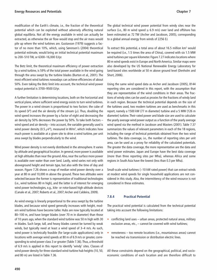
Energy Resources and Potentials Chapter 7
490
modification of the Earth’s climate, i.e., the fraction of the theoretical potential which can be exploited without adversely affecting natural global equilibria. Not all the energy available in wind can actually be extracted, as otherwise the air flow would stop and the air mass would pile up where the wind turbines are. Gustavson ( 1979 ) suggests a fac-tor of no more than 10%, which, using S ø rensen’s ( 2004 ) theoretical potential estimate, would bring an initial technical potential maximum to 200–510 TW, or 6300–16,000 EJ/yr.
The Betz limit, the theoretical maximum efficiency of power extraction by a wind turbine, is 59% of the total power available in the wind going through the area swept by the turbine blades (Burton et al., 2001 ). The most efficient wind turbines nowadays can achieve efficiencies of about 50%. Even taking the Betz limit into account, the technical wind power output potential is 3700–9500 EJ/yr.
A further limitation is determining locations, both on the horizontal and vertical plane, where sufficient wind energy exists to turn wind turbines. The power in a wind stream is proportional to two factors: the cube of its speed ( V 3 ) and the air density of the stream ( ρ ). Thus, doubling the wind speed increases the power by a factor of eight and decreasing the air density by 50% decreases the power by 50%. To take both factors – wind speed and air density – into account, the variable generally used is wind power density (0.5 ρ V 3 ), measured in W/m 2 , which indicates how much power is available at a given site to drive a wind turbine, per unit area swept by blades perpendicularly to the wind.
Wind power density is not evenly distributed in the atmosphere. It varies by altitude and geographical location. In general, more power is available at high altitudes than near the ground. Also, near the surface more power is available over water than over land. Lastly, wind varies not only with aboveground height and terrain type, but also with the time of day and season. Figure 7.26 shows a map of median wind power density over a year at 80 m and 10,000 m above the ground. These two altitudes were selected because the former is representative of traditional technologies (i.e., wind turbines 80 m high), and the latter is of interest for emerging wind power technologies, e.g., kite- or rotor-based high-altitude devices (Canale et al., 2007 ; Roberts et al., 2007 ; Archer and Caldeira, 2009 ).
As wind energy is linearly proportional to the area swept by the turbine blades, and because wind speed generally increases with height, mod-ern wind turbines have become taller. Hubs are now typically located at 80–100 m, and have longer blades (over 70 m in diameter) than those of 10 years ago, when the standard wind turbine was 50 m high with 30 m blades. Such large, tall, and heavy blades cannot be turned by weak winds, but typically need at least a wind speed of 3–4 m/s. As such, wind power is technically feasible (for large-scale applications) only in locations with average wind speeds at 80 m of 6.9 m/s or greater, corre-sponding to wind power class 3 or greater ( Table 7.36 ). Thus, a threshold of 6.9 m/s is applied in this report to identify ‘windy’ sites. Classes of wind power density for three standard wind-turbine hub heights (10, 50, and 80 m) are listed in Table 7.36 .
The global technical wind power potential from windy sites near the surface (i.e., 80 m wind speed ≥ 6.9 m/s) over land and offshore has been estimated as 72 TW (Archer and Jacobson, 2005 ), corresponding to a global annual energy from winds of 2256 EJ.
To extract this potential, a total area of about 16.5 million km 2 would be required (i.e., 1.5 times the area of China), covered with six 1.5 MW wind turbines per square kilometer. Figure 7.27 indicates locations where 80 m wind speeds exist in Europe and North America. Similar maps were also developed by the US National Renewable Energy Laboratory for land-based sites worldwide at 50 m above ground level (Denholm and Short, 2006 ).
Using the same wind speed data as Archer and Jacobson ( 2005 ), 8144 reporting sites are considered in this report, with the assumption that they are representative of the wind conditions in their areas. The frac-tions of windy sites can be used as proxies for the fractions of windy land in each region. Because the technical potential depends on the size of the turbines used, two modern turbines are used as benchmarks in this report, namely a 1500 kW (77 m diameter) turbine and a 5 MW (126 m diameter) turbine. Their rated power and blade size are used to calculate the yearly average wind power output as a function of the yearly average wind speed via the method in Jacobson and Masters ( 2001 ). Table 7.37 summarizes the values of relevant parameters in each of the 18 regions, including the range of technical potentials obtained from the two wind turbines. The data coverage, i.e., the number of reporting sites per unit area, can be used as a proxy for reliability of the calculated potentials. The greater the data coverage, the more representative are the data and wind power estimates. Japan and Europe have the best data coverage (more than three reporting sites per Mha), whereas Africa and some regions in South Asia have the lowest (less than 0.3 per Mha).
Small-scale wind turbines (~10 kW rated power) that can extract winds at modest wind speeds for single household applications are not con-sidered in this study. Also, the intermittency of the wind resource is not considered in these estimates.
7.8.4 Practical Potential
The practical wind potential is calculated from the technical potential taking into account the following limitations:
conflicting land uses – urban areas, protected natural areas, military •exclusion areas, etc., – cannot be covered with wind turbines;
remoteness – too remote locations (i.e., mountainous areas) cannot •be reached via transmission or distribution electric lines.
All these constraints depend on the geographical, political, and socio-economic conditions of each location and are therefore difficult to
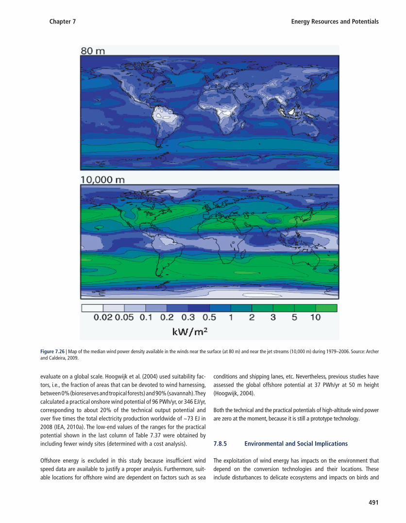
Chapter 7 Energy Resources and Potentials
491
evaluate on a global scale. Hoogwijk et al. ( 2004 ) used suitability fac-tors, i.e., the fraction of areas that can be devoted to wind harnessing, between 0% (bioreserves and tropical forests) and 90% (savannah). They calculated a practical onshore wind potential of 96 PWh/yr, or 346 EJ/yr, corresponding to about 20% of the technical output potential and over five times the total electricity production worldwide of ~73 EJ in 2008 (IEA, 2010a ). The low-end values of the ranges for the practical potential shown in the last column of Table 7.37 were obtained by including fewer windy sites (determined with a cost analysis).
Offshore energy is excluded in this study because insufficient wind speed data are available to justify a proper analysis. Furthermore, suit-able locations for offshore wind are dependent on factors such as sea
conditions and shipping lanes, etc. Nevertheless, previous studies have assessed the global offshore potential at 37 PWh/yr at 50 m height (Hoogwijk, 2004 ).
Both the technical and the practical potentials of high-altitude wind power are zero at the moment, because it is still a prototype technology.
7.8.5 Environmental and Social Implications
The exploitation of wind energy has impacts on the environment that depend on the conversion technologies and their locations. These include disturbances to delicate ecosystems and impacts on birds and
Figure 7.26 | Map of the median wind power density available in the winds near the surface (at 80 m) and near the jet streams (10,000 m) during 1979– 2006 . Source: Archer and Caldeira, 2009 .

Energy Resources and Potentials Chapter 7
492
other wildlife. In addition, there are social concerns about noise pollu-tion and landscape aesthetics. However, as previously mentioned, the exploitation of wind energy resources depends entirely on conversion technologies. The environmental and social impacts of wind turbines are discussed further in Chapters 3 , 11, and 20.
7.8.6 Summary
The theoretical potential of wind energy was determined to lie in the range 110,000 ± 50,000 EJ/yr. Adding technical constraints, including fundamental conversion maximums, as well as wind power density minimums, a technical potential was estimated as 1500–5700 EJ/yr. Including the winds blowing across Antarctica adds approximately another 2100 EJ/yr. Finally, practical limitations on the technical potential
were imposed, which took converter performance characteristics, land use conflicts, and electricity transmission into account. The practical poten-tial for onshore wind utilization was thus found to be 250–1200 EJ/yr (or about 20,000–100,000 TWh of electricity per year).
7.9 Solar
7.9.1 Overview
Solar energy is by far the most abundant energy resource on Earth and is ubiquitous over the Earth’s surface. To put in perspective the enormity of the sun’s energy, the average irradiation that hits the Earth’s surface in one hour is about equal to that of the energy consumed by all human activities in a year (IEA, 2010c ). Solar energy conversion technologies
Table 7.36 | Defi nition of wind power classes.a
Wind power class
10 m above ground 50 m above ground 80 m above ground
Wind power density Wind speed Wind power density Wind speed Wind power density Wind speed
[W/m 2 ] [m/s] [W/m 2 ] [m/s] [W/m 2 ] [m/s]
1 <100 <4.4 <200 <5.6 <250 <5.9
2 100–150 4.4–5.1 200–300 5.6–6.4 250–375 5.9–6.9
3 150–200 5.1–5.6 300–400 6.4–7.0 375–500 6.9–7.5
4 200–250 5.6–6.0 400–500 7.0–7.5 500–625 7.5–8.1
5 250–300 6.0–6.4 500–600 7.5–8.0 625–750 8.1–8.6
6 300–400 6.4–7.0 600–800 8.0–8.8 750–1000 8.6–9.4
7 >400 >7.0 >800 >8.8 >1000 >9.4
a Wind speed is assumed to have a Rayleigh distribution and to increase with height according to the power law with a friction coeffi cient of 1/7 and air density of 1.225 g/m 3 .
Source: adapted from AWEA, 2010 .
Figure 7.27 | Maps of annual average 80 m wind speed derived from observations in Europe and North America. Only locations in class 3 or greater (green and black dots) are windy enough for wind power. Source: Archer and Jacobson, 2005 .
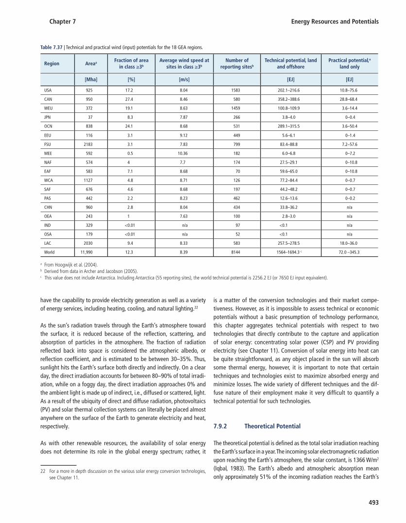
Chapter 7 Energy Resources and Potentials
493
have the capability to provide electricity generation as well as a variety of energy services, including heating, cooling, and natural lighting. 22
As the sun’s radiation travels through the Earth’s atmosphere toward the surface, it is reduced because of the reflection, scattering, and absorption of particles in the atmosphere. The fraction of radiation reflected back into space is considered the atmospheric albedo, or reflection coefficient, and is estimated to be between 30–35%. Thus, sunlight hits the Earth’s surface both directly and indirectly. On a clear day, the direct irradiation accounts for between 80–90% of total irradi-ation, while on a foggy day, the direct irradiation approaches 0% and the ambient light is made up of indirect, i.e., diffused or scattered, light. As a result of the ubiquity of direct and diffuse radiation, photovoltaics (PV) and solar thermal collection systems can literally be placed almost anywhere on the surface of the Earth to generate electricity and heat, respectively.
As with other renewable resources, the availability of solar energy does not determine its role in the global energy spectrum; rather, it
is a matter of the conversion technologies and their market compe-tiveness. However, as it is impossible to assess technical or economic potentials without a basic presumption of technology performance, this chapter aggregates technical potentials with respect to two technologies that directly contribute to the capture and application of solar energy: concentrating solar power (CSP) and PV providing electricity (see Chapter 11 ). Conversion of solar energy into heat can be quite straightforward, as any object placed in the sun will absorb some thermal energy, however, it is important to note that certain techniques and technologies exist to maximize absorbed energy and minimize losses. The wide variety of different techniques and the dif-fuse nature of their employment make it very difficult to quantify a technical potential for such technologies.
7.9.2 Theoretical Potential
The theoretical potential is defined as the total solar irradiation reaching the Earth’s surface in a year. The incoming solar electromagnetic radiation upon reaching the Earth’s atmosphere, the solar constant, is 1366 W/m2 (Iqbal, 1983 ). The Earth’s albedo and atmospheric absorption mean only approximately 51% of the incoming radiation reaches the Earth’s
Table 7.37 | Technical and practical wind (input) potentials for the 18 GEA regions.
Region Area a Fraction of area
in class ≥ 3 b Average wind speed at
sites in class ≥ 3 b Number of
reporting sites b Technical potential, land
and offshorePractical potential, a
land only
[Mha] [%] [m/s] [EJ] [EJ]
USA 925 17.2 8.04 1583 202.1–216.6 10.8–75.6
CAN 950 27.4 8.46 580 358.2–388.6 28.8–68.4
WEU 372 19.1 8.63 1459 100.8–109.9 3.6–14.4
JPN 37 8.3 7.87 266 3.8–4.0 0–0.4
OCN 838 24.1 8.68 531 289.1–315.5 3.6–50.4
EEU 116 3.1 9.12 449 5.6–6.1 0–1.4
FSU 2183 3.1 7.83 799 83.4–88.8 7.2–57.6
MEE 592 0.5 10.36 182 6.0–6.8 0–7.2
NAF 574 4 7.7 174 27.5–29.1 0–10.8
EAF 583 7.1 8.68 70 59.6–65.0 0–10.8
WCA 1127 4.8 8.71 126 77.2–84.4 0–0.7
SAF 676 4.6 8.68 197 44.2–48.2 0–0.7
PAS 442 2.2 8.23 462 12.6–13.6 0–0.2
CHN 960 2.8 8.04 434 33.8–36.2 n/a
OEA 243 1 7.63 100 2.8–3.0 n/a
IND 329 <0.01 n/a 97 <0.1 n/a
OSA 179 <0.01 n/a 52 <0.1 n/a
LAC 2030 9.4 8.33 583 257.5–278.5 18.0–36.0
World 11,990 12.3 8.39 8144 1564–1694.3 c 72.0 –345.3
a From Hoogwijk et al. ( 2004 ). b Derived from data in Archer and Jacobson ( 2005 ). c This value does not include Antarctica. Including Antarctica (55 reporting sites), the world technical potential is 2256.2 EJ (or 7650 EJ input equivalent).
22 For a more in depth discussion on the various solar energy conversion technologies, see Chapter 11 .
Energy Resources and Potentials Chapter 7
494
surface. The average irradiance thus reaching the surface is 697 W/m2, which multiplied by the Earth’s total land surface area results in a the-oretical potential estimate of 3,300,000 EJ/yr. Including the oceans, the total solar irradiation reaching the Earth is over 11,000,000 EJ/yr. These estimates, however, do not take into account localized weather conditions. Hoogwijk ( 2004 ) estimated the theoretical potential using a bottom-up approach with average irradiance data from the Climate Research Unit, which records empirical irradiation data for the past 30 years. This study estimates the theoretical input potential of solar energy to be lower, at around 630,000 EJ/yr.
7.9.3 Technical Potential
Several factors reduce the practically harvestable potential of this vast energy source. The amount of solar energy available at a given location is subject to daily and seasonal variations. Geographical variation is another important factor. Areas near the Equator generally receive more radiation than those at higher latitudes. Weather (atmospheric) conditions are typ-ically the strongest factors that influence solar energy availability. While solar tracking systems exist to reduce the impact of geographical varia-tions, these can only harvest direct sunlight, which is most affected by weather conditions. As irradiation is often diffuse, large-scale generation of solar energy can carry significant land requirements.
Siting issues combine with all three of the above factors. Not all surfaces are suitable for solar energy conversion, even if they have suitable geog-raphy and weather conditions. Land use conflicts (man-made infrastruc-ture, agriculture, or forests), geomorphology, topology, and protected or restricted areas pose siting constraints for larger solar installations. However, building structures provide interesting local siting possibilities for small-scale solar energy use.
These siting issues cause discrepancies in the various estimations of the global technical potential for solar energy, as different models have dif-ferent criteria and methods for assessing site suitability.
7.9.3.1 Direct Irradiation Potential
The German Aerospace Center (DLR) models the optical transparency of the atmosphere to calculate the direct normal irradiance (DNI) on the ground at any time and any site, by detecting and quantifying those atmospheric components that absorb or reflect the sunlight (clouds, aerosols, water vapor, ozone, and gases). The DNI serves as a reference for CSP systems and is defined as the solar radiation received per unit area by a surface that is always held normal, or perpendicular, to the rays that come in a straight line from the direction of the sun at its cur-rent position in the sky (DLR, 2009 ).
CSP systems track the sun using mirrors and lenses to concentrate the solar energy for the operation of steam cycles. Diffuse solar energy
cannot be used, as it has no uniform direction. Heat loss means that for CSP systems to operate efficiently, they require a minimum input of direct sunlight (IEA, 2010b ).
Thus, to plan a CSP plant, both site-specific radiation data and historical data are required to classify the actual ground-measurement radiation, taking year-to-year variations into account. Suitable areas, i.e., with high DNI, are usually found in arid and semiarid areas, between 15° and 40° latitude, and at higher altitudes, where both the air density and scatter-ing absorption are lower (IEA, 2010b ). In locations close to the equator it is too wet and cloudy during the rainy seasons, and nearer the poles it is often too cloudy. Figure 7.28 shows the DNI for 12 annual irradiation levels for the entire world.
Figure 7.28 shows that northern and southern Africa, the Middle East, parts of Chile, the southern United States, Mexico, and Australia are all suitable locations for CSP projects regarding DNI. The next constraint, then, is to find suitable land availability for the CSP systems. This is assessed by excluding land areas that are unsuitable because of ground structure, land cover, water bodies, slope, shifting sand, protected or restricted areas, forests, agriculture, urban areas, etc. The exclusion criteria can be strict and non-negotiable, or optional and thus subject to competition. Nevertheless, geographical characteristics and specific exclusion criteria, including competition for land use, jointly determine the viability of potential CSP project sites (Broesamle et al., 2001 ; Trieb et al., 2009 ).
Land areas with potentially suitable CSP sites, combined with the local DNI data, generate different classes of areas with a specific level of DNI. Table 7.38 shows the land area available for 13 DNI levels ranging from 1500–2800 kWh/m 2 /yr for all 18 GEA regions.
Most of the world’s regions, except for CAN, EEU, JPN, and PAS, have significant areas with good CSP potential. Although developers typic-ally set the bottom DNI threshold for CSP at 1900 kWh/m 2 /yr, locations with higher DNIs, everything else being equal, will be more econom-ically attractive. OCN, NAF, MEE, SAF, and OSA are regions where more than 50% of the CSP-suitable areas have DNI levels larger than 2300 kWh/m 2 /yr. Nevertheless, the global technical potential is found to be 277,000 EJ/yr. This is considered the available input energy for CSP systems worldwide.
In total, 33.6 million km 2 of land is technically suitable to host CSP systems, corresponding to about 26% of the world’s total land area. Without storage, CSP plants require around 2 ha/MWe, depending on the DNI and the technology. Even though the Earth’s ‘sunbelts’ are rela-tively narrow, the technical potential for CSP is huge. If fully developed for CSP applications, the potential in the southwestern United States alone would meet the electricity requirements of the entire United States several times over. Potential in the Middle East and North Africa would cover about 100 times the current demand of the Middle East, North Africa, and the EU combined (IEA, 2010b ).
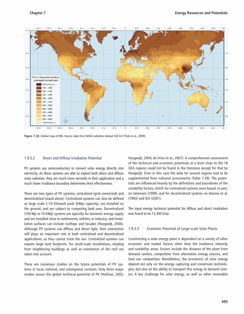
Chapter 7 Energy Resources and Potentials
495
7.9.3.2 Direct and Diffuse Irradiation Potential
PV systems use semiconductors to convert solar energy directly into electricity. As these systems are able to exploit both direct and diffuse solar radiation, they are much more versatile in their application and a much lower irradiance boundary determines their effectiveness.
There are two types of PV systems, centralized (grid connected) and decentralized (stand alone). Centralized systems can also be defined as large scale (>10 Kilowatt peak (kWp) capacity), are installed on the ground, and are subject to competing land uses. Decentralized (100 Wp to 10 kWp) systems are typically for domestic energy supply and are installed close to settlements, utilities, or industry, and instal-lation surfaces can include rooftops and facades (Hoogwijk, 2004 ). Although PV systems use diffuse and direct light, their orientation still plays an important role in both centralized and decentralized applications, as they cannot track the sun. Centralized systems can require large land footprints. For small-scale installations, shading from neighboring buildings as well as orientation of the roof are taken into account.
There are numerous studies on the future potentials of PV sys-tems in local, national, and subregional contexts. Only three major studies assess the global technical potential of PV (Hofman, 2002 ;
Hoogwijk, 2004 ; de Vries et al., 2007 ). A comprehensive assessment of the technical and economic potentials at a level close to the 18 GEA regions could not be found in the literature except for that by Hoogwijk. Even in this case the data for several regions had to be supplemented from national assessments ( Table 7.39 ). The poten-tials are influenced heavily by the definitions and boundaries of the suitability factors, which for centralized systems were based, in part, on S ø rensen ( 1999 ), and for decentralized systems on Alesma et al. ( 1993 ) and IEA ( 2001 ).
The input energy technical potential for diffuse and direct irradiation was found to be 12,300 EJ/yr.
7.9.3.3 Economic Potential of Large-scale Solar Plants
Constructing a solar energy plant is dependent on a variety of other economic and market factors other than the irradiance intensity and suitability areas. Factors include the distance of the plant from demand centers, competition from alternative energy sources, and land use competition. Nonetheless, the economics of solar energy depend not only on the energy capturing and conversion technolo-gies, but also on the ability to transport this energy to demand cent-ers. A key challenge for solar energy, as well as other renewable
Figure 7.28 | Global map of DNI. Source: data from NASA radiation dataset SSE 6.0 (Trieb et al ., 2009 ).

Energy Resources and Potentials Chapter 7
496
resources, is that electricity demand centers are not always situated close to the best sources.
7.9.4 Environmental and Social Implications
The environmental and social implications of solar energy depend on the technologies used and the amount of land covered. There is the potential concern of a significantly altered terrestrial albedo, particularly in regions where a lot of solar energy capture would exist. Land use con-flicts, particularly affecting soils and biodiversity (Dubreuil et al., 2007 ), and landscape aesthetics are social issues that could spark debate.
For CSP there are concerns over impacts on fragile desert ecosystems, although some systems could have a positive impact on the surrounding microclimate through enhanced shading (Tsoutsos et al., 2005 ). There is also the possibility of thermal pollution to water resources, especially in arid regions.
7.9.5 Summary
Solar energy is not only in itself directly the most abundant energy resource on Earth, but it is also indirectly responsible as the ultimate
source for hydro, wind, and, of course, biomass. The theoretical poten-tial of solar energy, taking weather conditions into account, is enor-mous at 630,000 EJ/yr, while the practical potential is estimated at 12,300 EJ/yr for PV applications and at 277,000 EJ/yr for CSP. However, offshore solar potential was not taken into account in this assessment, and neither was the potential of small PV (<10 kWp), as these systems have almost no land suitability issues and their potential is thus very difficult to characterize. The economic potential of solar energy relies heavily on conversion technologies, as well as localized factors such as siting and transmission issues, and these are not addressed in this assessment.
7.10 Geothermal Energy
7.10.1 Overview
Geothermal energy, in the broadest sense, is the natural heat of the Earth due to primarily the decay of the radioactive isotopes of uran-ium, thorium, and potassium. Immense amounts of thermal energy are generated and stored in the Earth’s core, mantle, and crust. At the base of the continental crust, temperatures range from 200–1000°C, and at the center of the Earth the temperatures may be in the range of 3500–5500°C (Alf é et al., 2001). The heat is transferred from the
Table 7.38 | Land areas suitable for CSP by direct normal irradiance.
DNI classes [kWh/m 2 /y]
1501–1600
1601–1700
1701–1800
1801–1900
1901–2000
2001–2100
2101–2200
2201–2300
2301–2400
2401–2500
2501–2600
2601–2700
2701–2800+
Total
[EJ/yr] [EJ/yr] [EJ/yr] [EJ/yr] [EJ/yr] [EJ/yr] [EJ/yr] [EJ/yr] [EJ/yr] [EJ/yr] [EJ/yr] [EJ/yr] [EJ/yr] [EJ/yr]
USA 539 151 383 1003 1173 1100 1371 1669 1280 1872 637 183 11,360
CAN 2 0.3 2
WEU 6 16 27 89 174 169 82 66 14 9 6 2 3 664
EEU 4 0.3 0.4 0.4 0.1 0.4 1 0.2 7
FSU 2508 1684 542 1018 1655 1109 24 29 14 5 8587
NAF 224 552 1052 1472 2157 2613 2556 7357 8787 7176 14,764 48,709
EAF 25 56 142 864 1560 1571 2040 2146 1506 1883 471 74 130 12,468
WCA 830 1245 1434 1805 2724 3914 5776 3906 5067 3985 2757 3736 8435 45,614
SAF 74 107 218 460 891 1023 1301 1781 1918 3201 3984 3024 3846 21,827
MEE 2 5 34 9 56 167 1098 2875 4711 5588 2742 2534 2894 22,716
CHN 346 524 84 177 297 651 1637 3150 2226 878 889 171 242 11,271
OEA 120 619 880 134 29 0 42 377 1700 441 163 20 4526
IND 2 18 99 250 534 616 89 43 60 33 1 9 1 1756
OSA 0.0 7 13 4 12 338 364 466 703 1,070 183 0.0 11 3171
JPN 9 0.4 0.3 0.0 10
PAS 173 118 123 140 64 13 9 3 1 1 645
OCN 19 60 38 155 538 517 1570 2753 6871 11,601 16,299 11,184 3897 55,501
LAC 1300 2492 3082 5246 3820 2598 1925 2114 2077 1732 848 523 1075 28,831
Total 5958 7102 7324 11,908 14,579 15,258 19,486 23,990 30,705 39,654 37,768 28,637 35,298 277,666
Source: Trieb et al., 2009 .

Chapter 7 Energy Resources and Potentials
497
interior toward the surface, mostly by conduction, and it this conduct-ive heat flow that causes a rise in temperature with increasing depth at a rate, on average, of 25–30°C/km. This is called the geothermal gradient. In the most promising locations, typically along fault lines, the average gradient can be up to 5–10 times the average, with very significant increases of temperature even at shallow depths.
Although the total heat content of the first few km under the Earth’s sur-face is immense, only a fraction can be utilized. Essentially, the Earth’s crust acts as an insulating blanket, which can best be accessed through fluid conduits, magma, water, etc., to exploit the underground energy and transfer it to the surface.
Despite the inherent uncertainties in developing estimates of geo-thermal potential, it is possible to identify a range of estimations, also taking into consideration the possibility of new technolo-gies, such as permeability enhancements, drilling improvements, enhanced geothermal system (EGS) technology, low temperature electricity production, and the use of supercritical fluids (Ledru et al., 2007 ).
7.10.2 Present Utilization of Geothermal Resources
Water from the deep wells and/or cold water from the surface is trans-ported through this deep reservoir using injection and production wells, and recovered as steam or hot water or both. Injection and production wells, and surface installations, complete the circulation system. The utilization of geothermal energy is divided into two categories, electri-city production and direct application, depending on fluid temperature.
Electricity is currently produced by geothermal energy in 24 countries. Five of these countries obtain 15–22% of their national electricity pro-duction from geothermal (Costa Rica, El Salvador, Iceland, Kenya, and the Philippines). There is ample opportunity for an increased use of geo-thermal energy both for direct applications and electricity production (Gawell et al., 1999 ).
Table 7.40 shows the recently observed rapid expansion in the utiliza-tion of geothermal energy for 18 world regions. In 2010, geothermal energy is expected to supply some 67 TWh/yr of electricity and 428 PJ/yr of heat for thermal applications (see Table 7.40 ).
Table 7.39 | Average irradiance, suitability factors, and solar energy input for PV for the 18 GEA regions.
Region Average
irradianceArea
Theoretical potential
Suitability factor
centralized
suitability factor
decentralized
Suitable area
centralized
Suitable area decentralized
Technical potential
centralized PV
Technical potential
decentralized PV
[W/m 2 ] [million km 2 ] [EJ/yr] [%] [%] [km 2 ] [km 2 ] [EJ] [EJ]
USA 127.4 9.2 37,003 0.92% 0.08% 84,640 7360 340.4 29.6
CAN 93.6 9.5 28,042 0.50% 0.01% 47,500 950 140.2 2.8
WEU 108.8 3.7 12,695 0.69% 0.26% 25,530 9620 87.6 33.0
EEU 124.4 1.2 4708 0.63% 0.08% 7560 960 29.7 3.8
FSU 95.8 21.8 65,861 0.92% 0.01% 199,470 2180 605.9 6.6
NAF 203.1 5.7 36,700 4.50% 0.01% 256,500 570 1651.5 3.7
EAF 184.1 11.3 65,605 2.10% 0.00% 237,300 283 1377.7 0.0
WCA 195.3 5.8 35,845 2.71% 0.00% 157,180 145 971.4 0.0
SAF 180.2 6.8 38,643 2.10% 0.01% 142,800 680 811.5 3.9
MEE 198.1 5.9 36,859 3.32% 0.03% 195,880 1770 1223.7 11.1
CHN a 167.5 8.3 43,843 2.14% 0.06% 178,155 4995 938.2 26.3
OEA 165.9 1.1 5886 0.51% 0.05% 5610 550 30.0 2.9
IND 200.7 2.8 17,722 2.14% 0.06% 59,385 1665 379.3 10.6
OSA 193.0 5.1 31,041 1.92% 0.05% 97,920 2550 596.0 15.5
JPN 126.4 0.4 1594 0.23% 1.21% 920 4840 3.7 19.3
OCN 188.5 8.4 49,934 3.32% 0.01% 278,880 840 1657.8 5.0
PAS 148.8 3.3 15,579 0.51% 0.05% 16,830 1650 79.5 7.8
LAC 164.2 20.3 105,351 1.11% 0.03% 185,100 4600 1169.4 31.6
World 153.7 130.6 632,912 1.69% 0.11% 2,177,160 46,208 12,093.5 213.4
a Irradiation data from Green Cross International ( 2009 ).
Source: adapted from Hoogwijk, 2004 .
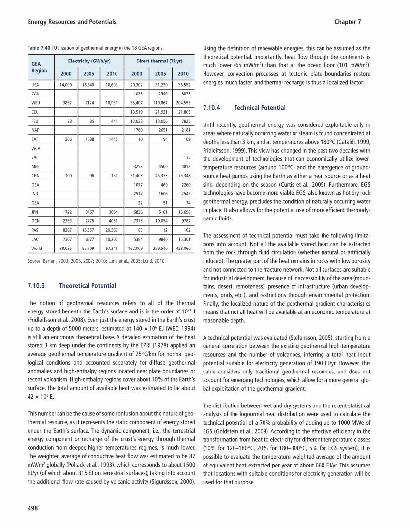
Energy Resources and Potentials Chapter 7
498
7.10.3 Theoretical Potential
The notion of geothermal resources refers to all of the thermal energy stored beneath the Earth’s surface and is in the order of 10 31 J (Fridleifsson et al., 2008 ). Even just the energy stored in the Earth’s crust up to a depth of 5000 meters, estimated at 140 × 10 6 EJ (WEC, 1994 ) is still an enormous theoretical base. A detailed estimation of the heat stored 3 km deep under the continents by the EPRI ( 1978 ) applied an average geothermal temperature gradient of 25°C/km for normal geo-logical conditions and accounted separately for diffuse geothermal anomalies and high-enthalpy regions located near plate boundaries or recent volcanism. High-enthalpy regions cover about 10% of the Earth’s surface. The total amount of available heat was estimated to be about 42 × 10 6 EJ.
This number can be the cause of some confusion about the nature of geo-thermal resource, as it represents the static component of energy stored under the Earth’s surface. The dynamic component, i.e., the terrestrial energy component or recharge of the crust’s energy through thermal conduction from deeper, higher temperatures regimes, is much lower. The weighted average of conductive heat flow was estimated to be 87 mW/m 2 globally (Pollack et al., 1993 ), which corresponds to about 1500 EJ/yr (of which about 315 EJ on terrestrial surfaces), taking into account the additional flow rate caused by volcanic activity (Sigurdsson, 2000 ).
Using the definition of renewable energies, this can be assumed as the theoretical potential. Importantly, heat flow through the continents is much lower (65 mW/m 2 ) than that at the ocean floor (101 mW/m 2 ). However, convection processes at tectonic plate boundaries restore energies much faster, and thermal recharge is thus a localized factor.
7.10.4 Technical Potential
Until recently, geothermal energy was considered exploitable only in areas where naturally occurring water or steam is found concentrated at depths less than 3 km, and at temperatures above 180°C (Cataldi, 1999 ; Fridleifsson, 1999 ). This view has changed in the past two decades with the development of technologies that can economically utilize lower-temperature resources (around 100°C) and the emergence of ground-source heat pumps using the Earth as either a heat source or as a heat sink, depending on the season (Curtis et al., 2005 ). Furthermore, EGS technologies have become more viable. EGS, also known as hot dry rock geothermal energy, precludes the condition of naturally occurring water in place. It also allows for the potential use of more efficient thermody-namic fluids.
The assessment of technical potential must take the following limita-tions into account. Not all the available stored heat can be extracted from the rock through fluid circulation (whether natural or artificially induced). The greater part of the heat remains in rocks with low porosity and not connected to the fracture network. Not all surfaces are suitable for industrial development, because of inaccessibility of the area (moun-tains, desert, remoteness), presence of infrastructure (urban develop-ments, grids, etc.), and restrictions through environmental protection. Finally, the localized nature of the geothermal gradient characteristics means that not all heat will be available at an economic temperature at reasonable depth.
A technical potential was evaluated (Stefansson, 2005 ), starting from a general correlation between the existing geothermal high-temperature resources and the number of volcanoes, inferring a total heat input potential suitable for electricity generation of 190 EJ/yr. However, this value considers only traditional geothermal resources, and does not account for emerging technologies, which allow for a more general glo-bal exploitation of the geothermal gradient.
The distribution between wet and dry systems and the recent statistical analysis of the lognormal heat distribution were used to calculate the technical potential of a 70% probability of adding up to 1000 MWe of EGS (Goldstein et al., 2009 ). According to the effective efficiency in the transformation from heat to electricity for different temperature classes (10% for 120–180°C, 20% for 180–300°C, 5% for EGS system), it is possible to evaluate the temperature-weighted average of the amount of equivalent heat extracted per year of about 660 EJ/yr. This assumes that locations with suitable conditions for electricity generation will be used for that purpose.
Table 7.40 | Utilization of geothermal energy in the 18 GEA regions.
GEA Region
Electricity (GWh/yr) Direct thermal (TJ/yr)
2000 2005 2010 2000 2005 2010
USA 14,000 16,840 16,603 20,302 31,239 56,552
CAN 1023 2546 8873
WEU 3852 7124 10,931 55,407 110,867 204,553
EEU 13,519 21,921 21,805
FSU 28 85 441 13,038 13,056 7825
NAF 1760 2651 2181
EAF 366 1088 1440 10 94 169
WCA
SAF 115
MEE 3253 4500 4812
CHN 100 96 150 31,403 45,373 75,348
OEA 1077 469 2260
IND 2517 1606 2545
OSA 22 51 74
JPN 1722 3467 3064 5836 5161 15,698
OCN 2353 2775 4056 7375 10,054 9787
PAS 8307 15,357 20,363 83 112 162
LAC 7307 8877 10,200 5384 9840 15,301
World 38,035 55,709 67,246 162,009 259,540 428,060
Source: Bertani, 2003 , 2005 , 2007 ; 2010 ; Lund et al., 2005 ; Lund, 2010 .
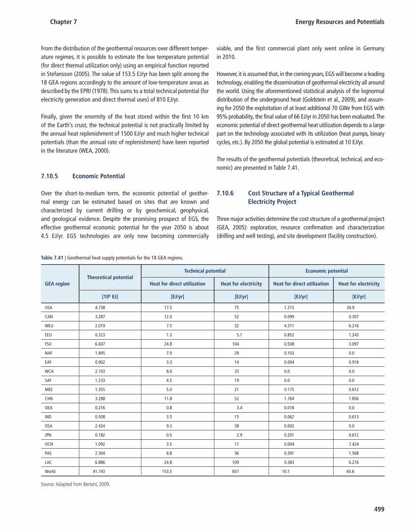
Chapter 7 Energy Resources and Potentials
499
From the distribution of the geothermal resources over different temper-ature regimes, it is possible to estimate the low temperature potential (for direct thermal utilization only) using an empirical function reported in Stefansson ( 2005 ). The value of 153.5 EJ/yr has been split among the 18 GEA regions accordingly to the amount of low-temperature areas as described by the EPRI ( 1978 ). This sums to a total technical potential (for electricity generation and direct thermal uses) of 810 EJ/yr.
Finally, given the enormity of the heat stored within the first 10 km of the Earth’s crust, the technical potential is not practically limited by the annual heat replenishment of 1500 EJ/yr and much higher technical potentials (than the annual rate of replenishment) have been reported in the literature (WEA, 2000).
7.10.5 Economic Potential
Over the short-to-medium term, the economic potential of geother-mal energy can be estimated based on sites that are known and characterized by current drilling or by geochemical, geophysical, and geological evidence. Despite the promising prospect of EGS, the effective geothermal economic potential for the year 2050 is about 4.5 EJ/yr. EGS technologies are only now becoming commercially
viable, and the first commercial plant only went online in Germany in 2010.
However, it is assumed that, in the coming years, EGS will become a leading technology, enabling the dissemination of geothermal electricity all around the world. Using the aforementioned statistical analysis of the lognormal distribution of the underground heat (Goldstein et al., 2009 ), and assum-ing for 2050 the exploitation of at least additional 70 GWe from EGS with 95% probability, the final value of 66 EJ/yr in 2050 has been evaluated. The economic potential of direct geothermal heat utilization depends to a large part on the technology associated with its utilization (heat pumps, binary cycles, etc.). By 2050 the global potential is estimated at 10 EJ/yr.
The results of the geothermal potentials (theoretical, technical, and eco-nomic) are presented in Table 7.41 .
7.10.6 Cost Structure of a Typical Geothermal Electricity Project
Three major activities determine the cost structure of a geothermal project (GEA, 2005 ): exploration, resource confirmation and characterization (drilling and well testing), and site development (facility construction).
Table 7.41 | Geothermal heat supply potentials for the 18 GEA regions.
GEA regionTheoretical potential
Technical potential Economic potential
Heat for direct utilization Heat for electricity Heat for direct utilization Heat for electricity
[10 6 EJ] [EJ/yr] [EJ/yr] [EJ/yr] [EJ/yr]
USA 4.738 17.5 75 1.215 34.9
CAN 3.287 12.0 52 0.099 0.307
WEU 2.019 7.5 32 4.311 6.216
EEU 0.323 1.3 5.1 0.852 1.243
FSU 6.607 24.8 104 0.508 3.097
NAF 1.845 7.0 29 0.103 0.0
EAF 0.902 3.3 14 0.004 0.918
WCA 2.103 8.0 33 0.0 0.0
SAF 1.233 4.5 19 0.0 0.0
MEE 1.355 5.0 21 0.175 0.612
CHN 3.288 11.8 52 1.764 1.856
OEA 0.216 0.8 3.4 0.018 0.0
IND 0.938 3.5 15 0.062 0.613
OSA 2.424 9.3 38 0.002 0.0
JPN 0.182 0.5 2.9 0.201 0.612
OCN 1.092 3.5 17 0.004 7.424
PAS 2.304 8.8 36 0.391 1.568
LAC 6.886 24.8 109 0.383 6.216
World 41.743 153.5 657 10.1 65.6
Source: Adapted from Bertani, 2009 .
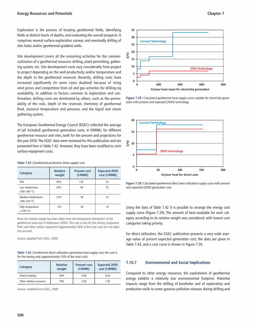
Energy Resources and Potentials Chapter 7
500
Exploration is the process of locating geothermal fields, identifying fields at distinct levels of depths, and evaluating the overall prospects. It comprises several surface exploration surveys and eventually drilling of slim holes and/or geothermal gradient wells.
Site development covers all the remaining activities for the commer-cialization of a geothermal resource: drilling, plant permitting, gather-ing system, etc. Site development costs vary considerably from project to project depending on the well productivity and/or temperature and the depth to the geothermal reservoir. Recently, drilling costs have increased significantly (in some cases doubled) because of rising steel prices and competition from oil and gas activities for drilling-rig availability. In addition to factors common to exploration and con-firmation, drilling costs are dominated by others, such as the perme-ability of the rock, depth of the reservoir, chemistry of geothermal fluid, resource temperature and pressure, and the liquid and steam gathering system.
The European Geothermal Energy Council (EGEC) collected the average of (all included) geothermal generation costs, in € /MWh, for different geothermal resource and sites, both for the present and projections for the year 2050. The EGEC data were reviewed for this publication and are presented here in Table 7.42 . However, they have been modified to omit surface-equipment costs.
Using the data of Table 7.42 it is possible to arrange the energy cost supply curve ( Figure 7.29 ). The amount of heat available for each cat-egory according to its relative weight was considered, with lowest cost categories taking priority.
For direct utilization, the EGEC publication presents a very wide aver-age value of present expected generation cost; the data are given in Table 7.43 , and a cost curve is shown in Figure 7.30 .
7.10.7 Environmental and Social Implications
Compared to other energy resources, the exploitation of geothermal energy exhibits a relatively low environmental footprint. Potential impacts range from the drilling of boreholes and of exploratory and production wells to some gaseous pollution releases during drilling and
0
5
10
15
20
0 50 100 150 200
$/G
J
EJ/year heat for direct uses
2050 Technology
Current Technology
Figure 7.30 | Calculated geothermal direct heat utilization supply curve with present and expected (2050) generation cost.
0
5
10
15
20
25
30
35
0 200 400 600 800
$/G
J
EJ/year heat input for electricity genera�on
Current Technology
2050 Technology
Figure 7.29 | Calculated geothermal heat supply curve suitable for electricity gener-ation with present and expected (2050) technology.
Table 7.43 | Geothermal direct utilization generation heat supply cost; the cost is for the mining only (approximately 10% of the total cost).
CategoryRelative weight
Present cost [ € /MWh]
Expected 2050 cost [ € /MWh]
District heating 30% 5.00 4.50
Other shallow resources 70% 2.00 1.50
Source: modifi ed from EGEC, 2009 .
Table 7.42 | Geothermal production (heat supply) cost.
CategoryRelative weight
Present cost [ € /MWh]
Expected 2050 cost [ € /MWh]
EGS 50% 120 25
Low temperature (100–180 °C)
33% 60 25
Medium temperature (180–250 °C)
12% 50 15
High temperature (>250 °C)
5% 30 10
Note: the relative weight has been taken from the temperature distribution of the geothermal resources of Stefansson ( 2005 ). This cost is only for the mining component. Plant and other surface equipment (approximately 50% of the total cost) are not taken into account.
Source: adapted from EGEC, 2009 .

Chapter 7 Energy Resources and Potentials
501
field testing. The installation pipelines may incur similar environmental impacts to those of drilling.
During plant operation, geothermal fluids (steam or hot water) usu-ally contain gases as well as dissolved chemicals, the concentrations of which usually increase with temperature – with H 2 S being one of the main pollutants. Various processes exist, however, that can reduce emissions significantly. Waste waters from geothermal plants also have higher temperatures than the surrounding environment and are therefore a potential thermal pollutant. The total reinjection of the used geothermal fluid is able to reduce strongly any impact of any potential liquid pollution. Adopting closed-loop systems essentially avoids any gaseous emissions.
The extraction of large quantities of fluids from geothermal reservoirs may give rise to subsidence phenomena, i.e., a gradual sinking of the land surface. This is a slow process distributed over vast areas and represents a low risk, if any. It takes years before such effects can be detected, but they need to be monitored systematically, as subsidence could damage the stability of buildings in the vicinity. In many cases subsidence can be prevented or reduced by reinjecting the geothermal waste waters.
The withdrawal and/or reinjection of geothermal fluids may trigger or increase the frequency of seismic events. However, these are microseis-mic events that can only be detected by means of instrumentation and to date no serious occurrence has been reported.
The high-pitched noise of steam traveling through pipelines and the occasional vent discharge are further potential adverse impacts. Finally, the scenic view can be affected adversely, although in some areas such as Larderello, Italy, the network of pipelines crisscrossing the country-side and the power-plant cooling towers have become an integral part of the panorama and are, indeed, a famous tourist attraction.
7.10.8 Summary
Geothermal energy is a renewable energy source that has been utilized economically in many parts of the world for decades. A great potential for an extensive increase in worldwide geothermal utilization exists, because new technologies allow for the exploitation of geothermal energy in many more locations. Still, the limiting factor for geothermal development rests in its geographical distribution, as high temperature gradients are available only in limited locations, even if the increas-ing role of binary fluids can strongly enlarge the possibility of using medium-to-low temperature areas.
The theoretical geothermal potential is not considered as the static heat content within the Earth’s crust, but the conductive heat flow from deeper, higher temperature areas, and is estimated at 1500 EJ/yr. Extracting more than this theoretical potential would result in a
progressive cooling of the Earth’s crust, and would no longer meet the principles of a renewable energy source. The technical potential was estimated to be 720 EJ/yr. This value approaches the upper limits of pre-vious assessments of geothermal potential, as aggregated in Bertani ( 2003 ). This is because the current estimation assumes the inclusion of dry-rock system extraction technologies, which can exploit the gen-eral geothermal gradient and are not dependent on existing, naturally occurring fluids. The economic potential, 75 EJ/yr, takes into account the limited number of areas suitable for geothermal extraction due to geo-logical constraints.
7.11 Ocean energy
7.11.1 Overview
Ocean energy refers to the kinetic energy carried by the waves, currents, and tides, as well as the potential energy stored in the ocean’s salinity and temperature differences. The oceans are a tremendous source of energy, especially as many of the world’s most concentrated popula-tions are located close by. Ocean energy resources have an advantage in that they are more reliably available, especially compared to solar and wind.
7.11.2 Ocean Thermal Energy Conversion
Ocean thermal energy conversion (OTEC) takes advantage of the tem-perature difference that results from solar radiation warming the surface water and cooler deeper ocean currents. By using a heat engine, this natural temperature difference can be exploited to produce electricity.
The oceans are the world’s largest solar energy collector and energy storage system. Although the average solar irradiation absorbed by the ocean is around 240 W/m 2 , Vega ( 1995 ) used an estimate of the average solar flux as 95 W/m 2 , which corresponds to the latent heat flux of the ocean. Using this average over the 360 million square-kilometer area of the Earth’s oceans, the total theoretical potential of ocean thermal energy is estimated to be 1,000,000 EJ/yr.
However, as with any heat engine, larger temperature differences gen-erate greater conversion efficiencies. A temperature difference of about 20 °C between the surface and 1000 m depth is required for OTEC sys-tems to produce significant quantities of power (Binger, 2010). Figure 7.31 shows a world map indicating the ocean temperatures gradients.
The temperature irradiance generally increases with decreasing lati-tude, i.e., it is greatest near the equator. Various studies have estimated
23 These potentials are the input energy and do not include electricity-conversion effi ciencies.
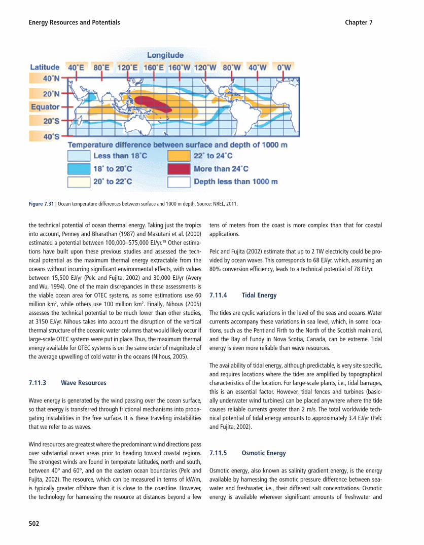
Energy Resources and Potentials Chapter 7
502
the technical potential of ocean thermal energy. Taking just the tropics into account, Penney and Bharathan ( 1987 ) and Masutani et al. (2000) estimated a potential between 100,000–575,000 EJ/yr. 19 Other estima-tions have built upon these previous studies and assessed the tech-nical potential as the maximum thermal energy extractable from the oceans without incurring significant environmental effects, with values between 15,500 EJ/yr (Pelc and Fujita, 2002 ) and 30,000 EJ/yr (Avery and Wu, 1994 ). One of the main discrepancies in these assessments is the viable ocean area for OTEC systems, as some estimations use 60 million km 2 , while others use 100 million km 2 . Finally, Nihous ( 2005 ) assesses the technical potential to be much lower than other studies, at 3150 EJ/yr. Nihous takes into account the disruption of the vertical thermal structure of the oceanic water columns that would likely occur if large-scale OTEC systems were put in place. Thus, the maximum thermal energy available for OTEC systems is on the same order of magnitude of the average upwelling of cold water in the oceans (Nihous, 2005 ).
7.11.3 Wave Resources
Wave energy is generated by the wind passing over the ocean surface, so that energy is transferred through frictional mechanisms into propa-gating instabilities in the free surface. It is these traveling instabilities that we refer to as waves.
Wind resources are greatest where the predominant wind directions pass over substantial ocean areas prior to heading toward coastal regions. The strongest winds are found in temperate latitudes, north and south, between 40° and 60°, and on the eastern ocean boundaries (Pelc and Fujita, 2002 ). The resource, which can be measured in terms of kW/m, is typically greater offshore than it is close to the coastline. However, the technology for harnessing the resource at distances beyond a few
tens of meters from the coast is more complex than that for coastal applications.
Pelc and Fujita ( 2002 ) estimate that up to 2 TW electricity could be pro-vided by ocean waves. This corresponds to 68 EJ/yr, which, assuming an 80% conversion efficiency, leads to a technical potential of 78 EJ/yr.
7.11.4 Tidal Energy
The tides are cyclic variations in the level of the seas and oceans. Water currents accompany these variations in sea level, which, in some loca-tions, such as the Pentland Firth to the North of the Scottish mainland, and the Bay of Fundy in Nova Scotia, Canada, can be extreme. Tidal energy is even more reliable than wave resources.
The availability of tidal energy, although predictable, is very site specific, and requires locations where the tides are amplified by topographical characteristics of the location. For large-scale plants, i.e., tidal barrages, this is an essential factor. However, tidal fences and turbines (basic-ally underwater wind turbines) can be placed anywhere where the tide causes reliable currents greater than 2 m/s. The total worldwide tech-nical potential of tidal energy amounts to approximately 3.4 EJ/yr (Pelc and Fujita, 2002 ).
7.11.5 Osmotic Energy
Osmotic energy, also known as salinity gradient energy, is the energy available by harnessing the osmotic pressure difference between sea-water and freshwater, i.e., their different salt concentrations. Osmotic energy is available wherever significant amounts of freshwater and
Figure 7.31 | Ocean temperature differences between surface and 1000 m depth. Source: NREL, 2011 .

Chapter 7 Energy Resources and Potentials
503
seawater come into contact, e.g., estuaries. The global discharge of freshwater to the seas is about 44,500 km 3 /yr. Using a potential energy of 2.35 MJ/s/m 3 of freshwater (van den Ende and Groeman, 2007 ), a theoretical potential of 105 EJ/yr is determined. Van den Ende and Groeman ( 2007 ) assume that about 10% would be considered technic-ally feasible, leading to a technical potential of 10 EJ/yr.
7.11.6 Environmental and Social Implications
The exploitation of ocean energy, as with any energy resource, is not without its downsides. For very large OTEC systems, thermal pollution, toxic releases, and impingement and entrainment of organisms on the plant itself pose potentially harmful sources. While the magnitude of thermal pollution would be small, even 3°C shifts in temperatures are known to cause high mortality to corals and fishes (Hoegh-Guldberg et al., 2007 ). Sensitive ecosystems could be affected further through nutrient loading caused by the drawing of deep coldwater. OTEC systems also release a small amount of CO 2 , because gas solubility is reduced in warmer water. OTEC systems have the greatest potential for small island developing states, which need both a reliable energy source and fresh-water (Binger, 2010).
Large-scale wave energy systems have the potential to disturb ocean ecosystems and harm marine life. They may also have a significant impact on ocean-atmospheric interactions. Wave energy devices alter the ocean’s currents, typically slowing them down and calming the sea. While this could be used in conjunction with wave-break systems, especially around harbors, it will cause reduced mixing of ocean layers,
and could reduce food supplies, particularly for bottom feeders. Finally, dampened waves could alter erosion patterns of the coastline, in either a positive or negative way, depending on location (Boehlert et al., 2008 ).
Tidal barrages could pose threats to sensitive ecosystems, especially in estuaries, by altering the flow of saltwater. Ecosystems could be further affected by slower currents, reduction of the intertidal area, and limited ocean layer mixing. Tidal turbines, however, are more benign. Although they could be potentially dangerous to fish and crustaceans, slow-turn-ing turbines could allow fish to swim through, and larger sea-life could be protected by undersea fences or nets (Boehlert and Gill, 2010 ).
As the main discharge waste of osmotic energy systems is brackish water, discharges of brackish water could cause salinity fluctuations outside those typical of the ecosystems, and so lead to loss of biodiver-sity. There is also the danger of impingement and entrainment of marine and estuarine organisms.
7.11.7 Summary
As the ocean covers almost 75% of the Earth’s surface, it is Earth’s larg-est collector of solar energy. This thermal potential accounts by far for the largest share of theoretical and technical ocean potentials. Ocean resources have the advantage over other renewables in that they are often more reliable and predictable. While the resource potential may be more than sufficient to meet global requirements (total technical potential, 3240 EJ/yr), special care must be given with regard to ocean ecosystems.

Energy Resources and Potentials Chapter 7
504
References
Adhikari , B. K. , S. Barrington and J. Martinez , 2006 : Predicted growth of world
urban food waste and methane production. Waste Management Resources,
24 (5): 421 – 433 .
Aguilera , R. F. , R. G. Eggert , G. C. C. Lagos and J. E. Tilton , 2009 : Depletion and the
Future Availability of Petroleum Resources. The Energy Journal, 30 (1): 141 – 174 .
Ahlbrandt , T. and T. Klett , 2005 : Comparison of Methods Used to Estimate
Conventional Undiscovered Petroleum Resources: World Examples. Natural
Resources Research, 14 (3): 187 – 210 .
Aitken , C. M. , D. M. Jones , and S. R. Larter , 2004 : Anaerobic hydrocarbon biodeg-
radation in deep subsurface oil reservoirs. Nature, 431 (7006): 291 – 294 .
Aldhous , P. , P. McKenna , and C. Stier , 2010 : Gulf Leak: Biggest Spill may not be
Biggest Disaster. New Scientist, 2764 .
Aleklett , K. , M. H öö k , K. Jakobsson , M. Lardelli , S. Snowden , and B. S ö derbergh ,
2010 : The Peak of the Oil Age – Analyzing the world oil production Reference
Scenario in World Energy Outlook 2008. Energy Policy, 38 (3): 1398 – 1414 .
Alf è , D. , M. J. Gillan , and G. D. Price , 2002 : Composition and temperature of the
Earth ’ s core constrained by combining ab initio calculations and seismic data.
Earth and Planetary Science Letters, 195 (1–2): 91 – 98 .
Allsema , E. and M. van Brummelen , 1993 : Het Potentieel van PV-Systemen in
OECD Landen. Utrecht University, Department of Science, Technology and
Society : pp. 53 .
Altun , N. E. , C. Hicyilmaz , J.-Y. Hwang , A. S. Bagci , and M. V. Kok , 2006 : Oil
shales in the world and Turkey; reserves, current situation and future prospects:
a review. Oil Shale. A Scientifi c-Technical Journal (Estonian Academy Publishers),
23 (3): 211 – 227 .
Ananenkov , D. G. , 2007 : Role of Gas in Development of Global and Russian Fuel and
Energy Industry in XXI Century, Paper P-1. In Proceedings of the International
Conference on World Gas Resources and Reserves and Advanced Development
Technologies , VNIIGAZ , Moscow .
Antilla , P. , T. Karjalainen , and A. Asikainen , 2009 : Global Potential of Modern
Firewood. Finnish Forest Institute, Vantaa. www.metla.fi /julkaisut/workingpa-
pers/2009/mwp118.htm (accessed January 16, 2011).
Archer , C. L. and M. Z. Jacobson , 2005 : Evaluation of global wind power . J. Geophys .
Res., 110 (D12): D12110 .
Archer , C. L. and K. Caldeira , 2009 : Global Assessment of High-Altitude Wind
Power. Energies, 2 (2): 307 – 319 .
Arthur , J. D. , B. Bohm , and M. Layne , 2008 : Hydraulic Fracturing Considerations
for Natural gas Wells of the Marcellus Shale . In The Ground Water Protection
Council 2008 Annual Forum, Cincinnati, OH .
Asikainen , A. , H. Liiri , S. Peltola , T. Karjalainen , and J. Laitila , 2008 : Forest energy
potential in Europe (EU 27). Finnish Forest Institute, Vantaa. www.metla.fi /
julkaisut/workingpapers/2008/mwp069.htm (accessed November 25, 2010).
Atlas , R. M. and R. Bartha , 1992 : Hydrocarbon Biodegradation and Oil Spill
Bioremediation In Advances in Microbial Ecology . K. C. Marshall , (ed.), Plenum
Press , London , 13, pp. 282–338.
AUA (Australian Uranium Association) , 2009 : Uranium Stewardship – Best
Practice Guidelines for Uranium Exploration Date Accessed: 2010, April, 10,
www.aua.org.au/Content/ExplorationGuidelines.aspx.
Avery , W. H. and C. Wu , 1994 : Renewable Energy From the Ocean–A Guide to
OTEC, Johns Hopkins University Applied Physics Laboratory Series in Science and
Engineering , J. R. Apel ed., Oxford University Press , NY .
AWEA (American Wind Energy Association) , 2010 : Basic Principles of Wind
Resource Evaluation. www.awea.org/faq/basicwr.html (accessed on: March 30,
2010).
Bentley , R. W. and M. R. Smith , 2004 : World Oil Production Peak – A Supply-
Side Perspective. International Association for Energy Economics Newsletters,
13 (Third Quarter): 25 – 28 .
Berndes , G. , M. Hoogwijk , and R. van den Broek , 2003 : The contribution of bio-
mass in the future global energy supply: a review of 17 studie s . Biomass and
Bioenergy, 25 (1): 1 – 28 .
Berndes , G. , 2008 : Water demand for global bioenergy production: trends, risks and
opportunities . In Welt im Wandel: Zukunftsf ä hige Bioenergie und nachhaltige
Landnutzung, WBGU (Wissenschaftlicher Beirat der Bundesregierung Globale
Umwelt Ver ä nderungen , Berlin .
Bertani , R. , 2003 : What is Geothermal Potential? IGA News, ( 53 ): 1 – 3 .
Bertani , R. , 2005 : World geothermal power generation in the period 2001 – 2005.
Geothermics, 34 (6): 651 – 690 .
Bertani , R. , 2007 : World Geothermal Power Generation in 2007. In Proceedings of
the European Geothermal Congress . 30 May – 1 June, Unterhaching , Germany .
Bertani , R. , 2009 : Long-term Projections of Geothermal-electric Development in the
World. GeoTHERM Expo & Congress . March 5–6, 2009, Offenburg , Germany .
Bertani , R. , 2010 : Geothermal Power Generation in the World: 2005–2010: Update
Report. International Geothermal Association . Bochum , Germany .
BGR , 2007 : Reserves, Resources and Availability of Energy Resources 2006 . Annual
Report, Federal Institute for Geoscience and Natural Resources (BGR), Hannover,
Germany .
BGR , 2009 : Energierohstoffe 2009 – Reserven, Ressourcen, Verf ü gbarkeit . Annual
Report, Federal Institute for Geoscience and Natural Resources (BGR) , Hannover,
Germany .
BGR , 2010 : Reserves, Resources and Availability of Energy Resources . Annual Reports,
Federal Institute for Geoscience and Natural Resources (BGR) , Hannover,
Germany .
Bhattacharya , S. C. , 1991 : Characterization of Selected Agro-forestry Residues . In
Biocoal Technology and Economics, Bhattacharya S.C. and R. M. Shrestha , (eds.),
Regional Energy Resources Information Center (RERIC) , Bangkok .
Bhattacharya , S. C. , J. M. Thomas , and P. Abdul Salam , 1997 : Greenhouse gas
emissions and the mitigation potential of using animal wastes in Asia. Energy,
22 (11): 1079 – 1085 .
Biglarbigi , K. , H. Mohan and J. Killen , 2009 : USA, World Possess Rich Resource
Base. Oil & Gas Journal, 107 (3): 56 – 61 .
Binger , A. , 2004 : Potential and Future Prospects for Ocean Thermal Energy Conversion
(OTEC) In Small Islands Developing States (SIDS). UNESCO ( UN Education,
Scientifi c and Cultural Organisation ).
Boehlert , G. W. , G. R. McMurray , and C. E. Tortorici , (eds.), 2008 : Ecological
Effects of Wave Energy in the Pacifi c Northwest. NOAA Technical Memo NMFS-F/
SPO-92 . US Department of Commerce , Washington, DC .
Boehlert , G. W. and A. B. Gill , 2010 : Environmental and Ecological Effects of Ocean
Renewable Energy Development. Oceanography, 23 (2): 68 – 81 .
BP , 2010 : Statistical Review of World Energy . BP , London .
Chapter 7 Energy Resources and Potentials
505
Broesamle , H. , H. Mannstein , C. Schillings , and F. Trieb , 2001 : Assessment of
solar electricity potentials in North Africa based on satellite data and a geo-
graphic information system. Solar Energy, 70 (1): 1 – 12 .
Bunn , M. , S. Fetter , J. P. Holdren , and B. van der Zwaan , 2003 : The Economics of
Reprocessing vs. Direct Disposal of Spent Nuclear Fuel. Project on Managing the
Atom. DE-FG26–99FT4028, Belfer Center for Science and International Affairs ,
John F. Kennedy School of Government, Harvard University , Cambridge, MA .
Burton , T. , D. Sharpe , N. Jenkins , and E. Bossanyi , 2001 : Wind Energy Handbook .
John Wiley & Sons , Hoboken , NJ .
Butler , R. M. and D. J. Stephens , 1980 : The Gravity Drainage of Steam-Heated Heavy
Oil to Parallel Horizontal Wells; Paper CIM # 80–31–31 . In Presented at the 31st
Petroleum Society of CIM Annual Technical Meeting, 25–28 May, Calgary .
Butler , R. M. and D. J. Stephens , 1981 : The Gravity Drainage of Steam-heated Heavy
Oil to Parallel Horizontal Wells. Journal of Canadian Petroleum Technology, 2 (2):
90 – 96 .
Campbell , C. J. and J. H. Laherr è re , 1998 : The End of Cheap Oil. Scientifi c American,
278 (3): 78 – 83 .
Campbell , J. E. , D. B. Lobell , R. C. Genova , and C. B. Field , 2008 : The Global
Potential of Bioenergy on Abandoned Agriculture Lands. Environmental Science
& Technology , 42 (15): 5791 – 5794 .
Canale , M. , L. Fagiano , and M. Milanese , 2007 : Power Kites for Wind Energy
Generation EEE Control Systems Magazine, pp. 25–38.
CAPP (Canadian Association of Petroleum Producers) , 2009 : Crude Oil: Forecast
Markets & Pipline Report. www.capp.ca/getdoc.aspx?DocId=173003 (accessed
May 5, 2011).
Cataldi , R. , 1999 : Geothermal development in Europe to the year 2020: prospects or
hopes? Technika Poszukiwa ń Geologicznych, 38 (4–5): 48 – 60 .
Cedigaz , 2009 : Natural Gas in the World . A. Lecarpentier , (ed.) Institut Fran ç ais du
P é trole, Rueil-Malmaison , France .
Charpentier , A. D. , J. A. Bergerson , and H. L. MacLean , 2009 : Understanding
the Canadian oil sands industry ’ s greenhouse gas emissions. Environmental
Research Letters, 4 (1): 014005 .
Cherubini , F. , N. D. Bird , A. Cowie , G. Jungmeier , B. Schlamadinger , and S.
Woess-Gallasch , 2009 : Energy- and greenhouse gas-based LCA of biofuel
and bioenergy systems: Key issues, ranges and recommendations. Resources,
Conservation and Recycling, 53 (8): 434 – 447 .
Chitrakar , R. , H. Kanoh , Y. Miyai , and K. Ooi , 2001 : Recovery of Lithium from Seawater
Using Manganese Oxide Adsorbent (H1.6Mn1.6O4) Derived from Li1.6Mn1.6O4.
Industrial & Engineering Chemistry Research, 40 (9): 2054 – 2058 .
Chum , H. , A. Faaij , J. Moreira , G. Berndes , P. Dhamija , H. Dong , B. Gabrielle , A.
Goss Eng , W. Lucht , M. Mapako , O. Masera Cerutti , T. McIntyre , T. Minowa ,
K. Pingoud , 2011 : Bioenergy. In IPCC Special Report on Renewable Energy
Sources and Climate Change Mitigation , O. Edenhofer , R. Pichs-Madruga , Y.
Sokona , K. Seyboth , P. Matschoss , S. Kadner , T. Zwickel , P. Eickemeier , G. Hansen ,
S. Schl ö mer , C. von Stechow (eds.), Cambridge University Press , Cambridge,
United Kingdom and New York, NY, USA .
Clarke , G. M. and P. W. Harben , 2009 : Lithium Availability Wall Map. www.lithi-
umalliance.org/about-lithium/lithium-sources/85-broad-based-lithium-reserves
(accessed January 3, 2011).
Clemens , J. , M. Triborn , P. Weiland , and B. Amon , 2005 : Mitigation of greenhouse
gas emissions by anaerobic digestion of cattle slurry. Agriculture, Ecosystems &
Environment, 112 (2–3): 171 – 177 .
Collett , T. S. , 2002 : Energy Resource Potential of Natural Gas Hydrates. AAPG
Bulletin, 86 (11): 1971 – 1992 .
Collett , T. S. , A. Johnson , C. C. Knapp , and R. Boswell , 2009 : Natural Gas Hydrates –
A Review. In Natural Gas Hydrates – Energy Resource Potential and Associated
Geologic Hazards . T. S. Collett , A. Johnson , C. C. Knapp and R. Boswell , (eds.),
American Association of Petroleum Geologists ; Memoir 89, pp. 137.
Couch , G. R. , 1988 : Lignite Resources and Characteristics, IEACR/13 . IEA Coal
Research , London, UK .
Crawford , P. M. , K. Biglarbigi , A. R. Dammer , and E. Knaus , 2008 : Advances in
World Oil Shale Production Technologies, SPE # 116570 In Presented at the 2008
Annual Technical Conference and Exhibition , 21–24 September, Denver, CO .
Crawford , P. M. , K. Biglarbigi , E. Knaus , and J. Killen , 2009 : New Approaches
Overcome Past Technical Issues. Oil & Gas Journal, 107 (4): 44 – 49 .
Curtis , R. , J. Lund , B. Sanner , L. Rybach , and G. Hellstr ö m , 2005 : Ground Source
Heat Pumps – Geothermal Energy for Anyone, Anywhere: Current Worldwide
Activity. In Proceedings of the World Geothermal Congress . April 24–29,
Antalya .
Daul , J. , 1995 : Untersuchung ü ber die Verteilung und Ver ä nderung der Steinkohlevorr ä te
im Ruhrgebiet und deren Ausnutzung . PhD-Thesis, Montanuniversit ä t Leoben ,
Leoben .
de Vries , B. J. M. , D. P. van Vuuren and M. M. Hoogwijk , 2007 : Renewable energy
sources: Their global potential for the fi rst-half of the 21st century at a global
level: An integrated approach. Energy Policy, 35 (4): 2590 – 2610 .
de Wit , M. and A. Faaij , 2010: European biomass resource potential and costs .
Biomass and Bioenergy , 34 (2): 188 – 202 .
Denholm , P. and W. Short , 2006 : Documentation of WinDS Base Case. Version AEO
2006 (1) . National Renewable Energy Laboratory , Golden, CO .
Deutsche Bank , 2009 : The Cost of Producing Oil. FITT Research . Deutsche Bank A.G. ,
London .
DLR (Deutsches Zentrum f ü r Luft- und Raumfahrt) , 2009 : Characterisation of
Solar Electricity Import Corridors from MENA to Europe – Potential, Infrastructure
and Cost . DLR , Stuttgart .
DOE (US Department of Energy) , 2010 : Enhanced oil Recovery/CO2 Injection.
http://fossil.energy.gov/programs/oilgas/eor/ (accessed March 20, 2011).
Dubreuil , A. , G. Gaillard , and R. M ü ller-Wenk , 2007 : Key Elements in a Framework
for Land Use Impact Assessment Within LCA (11 pp). The International Journal
of Life Cycle Assessment, 12 (1): 5 – 15 .
Dusseault , M. B. , 2002 : New Oil Production Technologies. SPE Distinguished Lectures
Series 2002–2003 . Paper SPE # 101463 DLP .
Dusseault , M. B. and A. Shafi ei , 2011 : Tar Sands. In Ullmann’s Encyclopedia of
Chemical Engineering , Wiley, Hoboken, NJ .
Dyni , J. R. , 2006 : Geology and Resources of Some World Oil-Shale Deposits. Scientifi c
Investigations Report 2005–5294 , US Geological Survey, Reston, VA .
E4Tech , 2009 : Biomass Supply Curves for the UK . E4Tech , London .
Earth Policy Institute , 2007 : Is World Oil Production Peaking? www.earth-policy.
org/Updates/2007/Update67_printable.htm (accessed November 30, 2010).
ECE (Economic Commission for Europe) , 2010 : United Nations International
Framework Classifi cation for Fossil Energy and Mineral Reserves and Resources
2009. The ECE Energy Series, No. 39, Economic Commission for Europe ,
Geneva .
EGEC (European Geothermal Energy Council) , 2009 : The Future of Geothermal
Development. EGEC -Renewable Energy House , Brussels , Belgium .

Energy Resources and Potentials Chapter 7
506
Ekins , P. , R. Vanner , and J. Firebrace , 2007 : Zero emissions of oil in water from
offshore oil and gas installations: economic and environmental implications.
Journal of Cleaner Production, 15 (13–14): 1302 – 1315 .
EPRI (Electric Power Research Institute) , 1978 : Geothermal energy prospects
for the next 50 years. Special Report ER-611-SR. www.osti.gov/energycitations/
servlets/purl/5027376-y14BJ4/ (accessed February 12, 2011).
Evans R. K. , 2008 : An Abundance of Lithium. www.che.ncsu.edu/ILEET/phevs/lith-
ium-availability/An_Abundance_of_Lithium.pdf (accessed April 20, 2010).
EWG (Energy Watch Group) , 2006 . Uranium Resources and Nuclear Energy, EWG-
Series No 1/2006 . Zittel W . And J. Schindler (eds.). Ludwig B ö lkow Systemtechnik
GmbH , Ottobrunn/Achen, Germany .
EWG (Energy Watch Group) , 2007 : Crude Oil: The Supply Outlook Report to the
Energy Watch Group. EWG-Series No 3/2007 , Ludwig-B ö lkow-Systemtechnik
GmbH , Ottobrunn .
EWG (Energy Watch Group) , 2008 : Zukunft der weltweiten Erd ö lversorgung .
Ludwig-B ö lkow-Systemtechnik GmbH , Ottobrunn .
Exxon , 2008 : Ö ldorado 2008 . Jubil ä um 50 Jahre, ExxonMobil , Hamburg .
FAO , 2006a : World agriculture: towards 2015/2030 – Interim report. Prospects for
food, nutrition, agriculture and major commodity groups . Food and Agricultural
Organization (FAO) , Rome .
FAO , 2006b : World agriculture: towards 2030/2050 – Interim report. Prospects for
food, nutrition, agriculture and major commodity groups . Food and Agricultural
Organization (FAO) , Rome .
FAO , 2006c : Gridded Livestock of the World . Food and Agricultural Organization (FAO) ,
Rome . http://www.fao.org/ag/AGAinfo/resources/en/glw/default.html (accessed
September 21, 2010).
FAO , 2009 : FAOSTAT 2009 . Food and Agricultural Organization (FAO) , Rome . http://
faostat.fao.org/site/573/default.aspx#ancor (accessed September 21, 2010).
Farrell , A. E. , 2008 : Energy Notes . News from the University of California Energy
Institute . Vol. 6 : p. 3 .
Fettweis , G. B. , 1976 : Weltkohlenvorr ä te. Eine vergleichende Analyse ihrer Erfassung
und Bewertung . Verlag Gl ü ckauf , Essen .
Fettweis , G. B. , 1990 : Der Produktionsfaktor Lagerst ä tte . In Bergwirtschaft. S. v.
Wahl , (ed.), Verlag Gl ü ckauf , Essen .
Field , C. B. , J. E. Campbell , and D. B. Lobell , 2008 : Biomass energy: the scale of the
potential resource. Trends in Ecology & Evolution, 23 (2): 65 – 72 .
Firbank , L. , 2008 : Assessing the Ecological Impacts of Bioenergy Projects. BioEnergy
Research, 1 (1): 12 – 19 .
Fischer , G. , E. Hizsnyik , S. Prieler , and H. van Velthuizen , 2007 : Assessment of
biomass potentials for bio-fuel feedstock production in Europe: Methodology
and results. REFUEL Project . International Institute for Applied Systems Analysis
(IIASA) , Laxenburg .
Florentinus , A. , C. Hamelinck , S. de Lint , and S. van Iersel , 2008 : Worldwide
Potential of Aquatic Biomass Ecofys , Utrecht .
Foley , J. A. , R. DeFries , G. P. Asner , C. Barford , G. Bonan , S. R. Carpenter , F. S.
Chapin , M. T. Coe , G. C. Daily , H. K. Gibbs , J. H. Helkowski , T. Holloway ,
E. A. Howard , C. J. Kucharik , C. Monfreda , J. A. Patz , I. C. Prentice , N.
Ramankutty , and P. K. Snyder , 2005 : Global Consequences of Land Use.
Science, 309 (5734): 570–574.
Fridleifsson , I. B. , 1999 : Worldwide Prospects for Geothermal Energy in the 21st
Century. Technika Poszukiwa ń Geologicznych, 38 (4–5): 28 – 34 .
Fridleifsson , I. B. , R. Bertani , E. Huenges , J. Lund , A. Ragnarsson , and
L. Rybach , 2008 : The Possible Role and Contribution of Geothermal Energy
to the Mitigation of Climate Change. In IPCC Scoping Meeting on Renewable
Energy Sources . 21–25 January, Lübeck .
Gawell , K. , M. Reed , and P. M. Wright , 1999 : Geothermal Energy: The Potential for
Clean Power from the Earth . Geothermal Energy Association , Washington, DC .
GEA (Geothermal Energy Association) , 2005 : Factors Affecting Costs of
Geothermal Power Development. Report for the US Department of Energy , US
Department of Energy , Washington, DC .
Gerbens-Leenes , W. , A. Y. Hoekstra , and T. H. van der Meer , 2009 : The water foot-
print of bioenergy. Proceedings of the National Academy of Sciences, 106 (25):
10219 – 10223 .
Gesamtverband Steinkohle , 2007 : Zahlen der Betribsstatistik . Annual Report,
Gesamtverband Steinkohle , Essen .
Gibbs , H. K. , M. Johnston , J. A. Foley , T. Holloway , C. Monfreda , N. Ramankutty ,
and D. Zaks , 2008 : Carbon payback times for crop-based biofuel expansion
in the tropics: the effects of changing yield and technology. Environmental
Research Letters, 3 (3): 034001 .
Gold , T. and S. Soter , 1980 : The Deep-earth Gas hypothesis. Scientifi c American,
242 (6): 155 – 161 .
Gold , T. and S. Soter , 1982 : Abiogenic Methane and the Origin of Petroleum. Energy
Exploration & Exploitation, 1 (2): 89 – 104 .
Gold , T. , 1988 : Origin of Petroleum: Two Opposing Theories and a Test in Sweden.
In The Methane Age . T. H. Linden , D. A. Dreyfus and T. Vasko , (eds.), Kluwer
Academic Publishers , Dordrecht .
Gold , T. , 1999 : The Deep Hot Biosphere . Springer , New York .
Goldstein , B. A. , A. J. Hill , A. Long , A. R. Budd , F. Holgate , and M. Malavos ,
2009 : Hot Rock Geothermal Energy Plays in Australia. In Proceedings of the
34th Workshop on Geothermal Reservoir Engineering . 9–11 February, Stanford
University Stanford, CA .
Graue , A. , B. Kvamme , B. A. Baldwin , J. Stevens , J. Howard , G. Ersland , J. Husebo ,
and D. R. Zornes , 2006 : Magnetic resonance imaging of methane – carbon
dioxide hydrate reactions in sandstone pores . Paper Number SPE 102915. In
Proceedings of the SPE Annual Technical Conference and Exhibition, 24–27
September, San Antonio, TX .
Green Cross International , 2009 : Global Solar Report Cards . Green Cross
International , Geneva .
Gruber P. and P. Medina , 2010 : Global Lithium Availability: A Constraint for Electric
Vehicles? MSc Thesis , Department of Natural Resources and Environment ,
University of Michigan .
Gustavson , M. R. , 1979 : Limits to Wind Power Utilization. Science, 204 (4388):
13 – 17 .
Haberl , H. , K.-H. Erb , F. Krausmann , W. Loibl , N. Schulz , and H. Weisz , 2001 :
Changes in ecosystem processes induced by land use: Human appropriation
of aboveground NPP and its infl uence on standing crop in Austria. Global
Biogeochem. Cycles, 15 (4): 929 – 942 .
Haberl , H. , K. H. Erb , F. Krausmann , V. Gaube , A. Bondeau , C. Plutzar , S.
Gingrich , W. Lucht , and M. Fischer-Kowalski , 2007a : Quantifying and
mapping the human appropriation of net primary production in earth ’ s terres-
trial ecosystems. Proceedings of the National Academy of Sciences, 104 (31):
12942 – 12947 .

Chapter 7 Energy Resources and Potentials
507
Haberl , H. , K. H. Erb , C. Plutzar , M. Fischer-Kowalski and F. Krausmann , 2007b :
Human Appropriation of Net Primary Production (HANPP) as Indicator for
pressures on Biodiversity. In Sustainability Indicators: A Scientifi c Assessment
(SCOPE) . T. Hak , B. Moldan and A. L. Dahl , (eds.), Island Press , Washington, DC .
Haberl , H. , V. Gaube , R. D í az-Delgado , K. Krauze , A. Neuner , J. Peterseil , C.
Plutzar , S. J. Singh and A. Vadineanu , 2009 : Towards an integrated model
of socioeconomic biodiversity drivers, pressures and impacts. A feasibility
study based on three European long-term socio-ecological research platforms.
Ecological Economics, 68 (6): 1797 – 1812 .
Hakala , K. , M. Kontturi and K. Pahkala , 2009 : Field Biomass as Global Energy
Source. Agricultural and Food Science, 18 : 347 – 368 .
Haq , Z. and J. Easterly , 2006 : Agricultural residue availability in the United States.
Applied Biochemistry and Biotechnology, 129 (1): 3 – 21 .
Harms , A. A. , D. R. Kingdon , K. F. Schoepf , and G. H. Miley , 2000 : Principles of
Fusion Energy . World Scientifi c Publishing Company , London .
HDWA (Hydropower and Dams World Atlas) , 2008 : Hydropower and Dams World
Atlas . The International Journal on Hydropower and Dams, Sutton : Aquamedia
Publications, Surrey, UK .
Head , I. M. , D. M. Jones , and S. R. Larter , 2003 : Biological activity in the deep
subsurface and the origin of heavy oil. Nature, 426 (6964): 344 – 352 .
Heinberg , R. and D. Fridley , 2010 : The end of cheap coal. Nature, 468 (7322):
367 – 369 .
Hirsch , R. L. , 2005 : Peaking of World Oil Production: Impacts, Mitigation, & Risk
Management. Association for the Study of Peak Oil and Gas . National Energy
Technology Laboratory .
Hoegh-Guldberg , O. , P. J. Mumby , A. J. Hooten , R. S. Steneck , P. Greenfi eld , E.
Gomez , C. D. Harvell , P. F. Sale , A. J. Edwards , K. Caldeira , N. Knowlton ,
C. M. Eakin , R. Iglesias-Prieto , N. Muthiga , R. H. Bradbury , A. Dubi , and
M. E. Hatziolos , 2007 : Coral Reefs Under Rapid Climate Change and Ocean
Acidifi cation. Science, 318 (5857): 1737 – 1742 .
Hofman , Y. , D. de Jager , E. Molenbroek , F. Schilig , and M. Voogt , 2002 : The
Potential Of Solar Electricity to Reduce CO2 Emissions . Ecofys , Utrecht .
Hoogwijk , M. , 2004 : On the global and regional potential of renewable energy
sources . Universiteit Utrecht , Utrecht .
Hoogwijk , M. , B. de Vries , and W. Turkenburg , 2004 : Assessment of the global
and regional geographical, technical and economic potential of onshore wind
energy. Energy Economics, 26 (5): 889 – 919 .
Hoogwijk , M. , A. Faaij , B. de Vries , and W. Turkenburg , 2009 : Exploration of
regional and global cost-supply curves of biomass energy from short-rotation
crops at abandoned cropland and rest land under four IPCC SRES land-use sce-
narios. Biomass and Bioenergy, 33 (1): 26 – 43 .
Hubbert , M. K. , 1971 : Energy Resources of the Earth. Scientifi c American, 224 (3):
60 – 70 .
IAASTD , 2009 . Agriculture at a Crossroads. International Assessment of Agricultural
Knowledge, Science and Technology for Development (IAASTD) , Global Report.
Island Press , Washington, DC .
IAEA (International Atomic Energy Agency) , 2005 : Thorium Fuel Cycle – Potential
Benefi ts and Challenges . IAEA-TECDOC-1350, Vienna .
IEA (International Energy Agency) , 2000 : Hydropower and the Environment:
Present context and guidelines for future action. Subtask 5 Report, Volume II:
Main Report , International Energy Agency of the Organisation of Economic
Co-Operation and Development , Paris .
IEA , 2001 : Potential for building integrated photovoltaics . International Energy
Agency of the Organisation of Economic Co-Operation and Development ,
Paris .
IEA , 2006a : World Energy Outlook 2006 . International Energy Agency of the
Organisation of Economic Co-Operation and Development , Paris .
IEA , 2006b : Energy Technology Perspectives 2006: Scenarios & Strategies to 2050 .
International Energy Agency of the Organisation of Economic Co-Operation and
Development , Paris .
IEA , 2007a : Energy Balances of Non-OECD Countries, 2004–2005 – 2007 Edition .
CD-ROM. International Energy Agency of the Organisation of Economic
Co-Operation and Development , Paris .
IEA , 2007b : Energy Balances of OECD Countries, 2004–2005 – 2007 Edition . CD-ROM.
International Energy Agency of the Organisation of Economic Co-Operation and
Development , Paris .
IEA , 2008a : World Energy Outlook 2008 . International Energy Agency of the
Organisation of Economic Co-Operation and Development , Paris .
IEA , 2008b : Renewables Information 2008 . International Energy Agency of the
Organisation of Economic Co-Operation and Development , Paris .
IEA , 2009 : World Energy Outlook 2009 . International Energy Agency of the
Organisation of Economic Co-Operation and Development , Paris .
IEA , 2010a : World Energy Outlook 2010 . International Energy Agency of the
Organisation of Economic Co-Operation and Development , Paris .
IEA , 2010b : Technology Roadmap: Concentrating Solar Power . International Energy
Agency of the Organisation of Economic Co-Operation and Development ,
Paris .
IEA , 2010c : Technology Roadmap: Solar Photovoltaic Energy . International Energy
Agency of the Organisation of Economic Co-Operation and Development , Paris .
IEA Coal , 1983 : Concise Guide to World Coal fi elds . International Energy Agency Coal
Research , London .
IGC (International Geological Congress) , 1913 : The Coal Resources of the World.
Enquiry made upon the initiative of the Executive Committee of the Twelfth
International Geological Congress , Morang & Co ., Toronto .
IGU (International Gas Union) , 1994 : Report of IGU Committee A (Production,
Treatment and Underground Storage of Natural Gas) 9.2 Production from Deep
Fields . IGU/A-94. In Proceedings of the19th World Gas Conference, 20–23 June,
Milan .
IGU , 2003 : Report of IGU Working Committee 1: Exploration, production and treat-
ment of natural gas . In 22nd World Gas Conference , 1–5 June, Tokyo .
IHS-CERA (Cambridge Energy Research Associates) , 2006 : Why the “ Peak Oil ”
Theory Falls Down Myths, Legends, and the Future of Oil Resources . P. Jackson
(ed.), CERA , Cambridge, MA .
IHS-CERA , 2010 : Oil Sands, Greenhouse Gases, and US Oil Supply. Special Report ,
IHS-CERA Inc ., Cambridge, MA .
IHS-CERA , 2011 : Oil Sands Technology, Past, Present and Future. Special Report , IHS
CERA Inc ., Cambridge, MA .
IPCC , 1996 : Climate Change 1995. In Adaptations and Mitigation of Climate Change:
Scientifi c-technical Analysis. Contribution of Working Group II to the Second
Assessment Report of the Intergovernmental Panel on Climate Change (IPCC) .
R. T. Watson , M. C. Zinyowera , and R. H. Moss , (eds.), Cambridge University Press ,
Cambridge, UK .
IPCC , 2006 : IPCC Guidelines for National Greenhouse Gas Inventories . Institute for
Global Environmental Strategies , Japan .

Energy Resources and Potentials Chapter 7
508
IPCC , 2007 : Mitigation of Climate Change. Contribution of working group III to
the Fourth Assessment report of the IPCC , B. Metz , O. R. Davidson , P. R. Bosch ,
R. Dave and L. A. Meyer , (eds.), Cambridge University Press , Cambridge, UK .
Iqbal , M. , 1983 : An Introduction to Solar Radiation . Academic Press , New York .
Jaccard , M. , 2006 : Sustainable Fossil Fuels: the Unusual Suspect in the Quest for
Clean and Enduring Energy . Cambridge University Press , Cambridge, UK .
Jacobson , M. Z. and G. M. Masters , 2001 : Exploiting wind versus coal. Science,
293 (5534): 1438 .
Jaksula , B. W. , 2008 : US Geological Survey Minerals yearbook – 2007 . US Geological
Survey , Washington, DC .
Jeglic , F. , 2004 : Analysis of Ruptures and Trends on Major Canadian Pipeline Systems .
National Energy Board of Canada , Calgary, AB .
Jekayinfa , S. O. and V. Scholz , 2007 : Assessment of availability and cost of energeti-
cally usable crop residues in Nigeria. In Conference on International Agricultural
Research for Development . 9–11 October, University of G ö ttingen .
Johansson , T.B. , Kelly H. , Reddy A.K.N. and H. Williams , (eds), 1993 : Renewable
Energy: Sources for Fuels and Electricity . Washington, DC : Island Press .
Johnston , M. , J. A. Foley , T. Holloway , C. J. Kucharik and C. Monfreda , 2009 :
Resetting global expectations from agricultural biofuels. Environmental Research
Letters, 4 (1): 01 4004 .
Junginger , M. , R. Sikkema and A. P. C. Faaij , 2009 : Analysis of the global pellet
market. Including major driving forces and possible technical and non-technical
barriers . Report for the Pellet@las project, Copernicus Institute , Utrecht .
Kato , T. , K. Okugawa , Y. Sugihara , and T. Matsumura , 1999 : Conceptual Design
of Uranium Recovery Plant from Seawater. Journal of the Thermal and Nuclear
Power Engineering Society, 50 (1): 71 – 77 .
Kenney , J. F. , 1996 : Considerations about recent predictions of impending short-
ages of petroleum evaluated from the perspective of modern petroleum science .
Special Edition on “The Future of Petroleum” in Energy World, British Institute
of Petroleum , London .
Kenney , J. F. , V. A. Kutcherov , N. A. Bendeliani , and V. A. Alekseev , 2002 : The
evolution of multicomponent systems at high pressures: VI. The thermodynamic
stability of the hydrogen-carbon system: The genesis of hydrocarbons and the
origin of petroleum. Proceedings of the National Academy of Sciences of the
United States of America, 99 (17): 10976 – 10981 .
Kenney , J. F. , V. I. Sozanksy , and P. M. Chepil , 2009 : On the Spontaneous Renewal
of Oil and Gas Fields. Energy Politics, XVII (Spring 2009 ).
Koopmans , A. and J. Koppejan , 1998 : Agricultural and forest residues – generation,
utilization and availability . In Regional Consultation on Modern Applications of
Biomass Energy, 6–10 January, Kuala Lumpur .
Krajick , K. , 2001 : Defending Deadwood. Science, 293 (5535): 1579 – 1581 .
Krausmann , F. , K.-H. Erb , S. Gingrich , C. Lauk , and H. Haberl , 2008 : Global
patterns of socioeconomic biomass fl ows in the year 2000: A comprehensive
assessment of supply, consumption and constraints. Ecological Economics,
65 (3): 471 – 487 .
Kudryavtsev , N. A. , 1951 : Against the Organic Hypothesis of Oil Origin. Oil Economy
Journal , ( 9 ): 17 – 29 .
Kundel , H. , 1985 : Face technology in German coal mines in 1984. In German
Longwall Mining – Facts and Figures. In Gl ü ckauf Bergbau Handbuch Nr . 32.,
Verlag Gl ü ckauf , Essen .
Laherr è re , J. H. , 2004 : Future of Natural Gas Supply. In Contribution to the 3rd
International Workshop on Oil&Gas Depletion . 24–25 May, Berlin .
Laherr è re , J. H. , 2005 : Review on Oil Shale Data. http://www.oilcrisis.com/laherrere/
OilShaleReview200509.pdf.
Lal , R. , 2004 : Agricultural activities and the global carbon cycle. Nutrient Cycling in
Agroecosystems, 70 (2): 103 – 116 .
Lal , R. , 2005 : World crop residues production and implications of its use as a biofuel.
Environment International, 31 (4): 575 – 584 .
Lal , R. , 2006 : Soil and Environmental Implications of Using Crop Residues as Biofuel
Feedstock. International Sugar Journal, 108 (1287): 161 – 167 .
Landsmann , H. , 2009 : Personal communication on soft brown coal mining cost
ranges.
Lauk , C. and K.-H. Erb , 2009 : Biomass consumed in anthropogenic vegetation fi res:
Global patterns and processes. Ecological Economics, 69 (2): 301 – 309 .
Ledru , P. , D. Bruhn , P. Calcagno , A. Genter , E. Huenges , M. Kaltschmitt ,
C. Karytsas , T. Kohl , L. Le Bel , A. Lokhorst , A. Manzella , and S. Thorhalsson ,
2007 : Enhanced Geothermal Innovative Network for Europe: The State-of-the-
Art . Geothermal Resources Council Bulletin , 36.
Lehner , B. , G. Czisch , and S. Vassolo , 2001 : Europe’s Hydropower Potential Today
and in the Future . EuroWasser, Center for Environmental Systems Research,
University of Kassel , Kassel .
Lemperiere , F. , 2006 : The Role of Dams in the XXI Century: Achieving a Sustainable
Development Target. International Journal on Hydropower & Dams, 13 (3):
98 – 108 .
Lewandowski , I. and A. P. C. Faaij , 2006 : Steps towards the development of a
certifi cation system for sustainable bio-energy trade. Biomass and Bioenergy,
30 (2): 83 – 104 .
Lewis , W. B. , 1972 : Energy in the Future: the Role of Nuclear Fission and Fusion .
Proceedings of the Royal Society of Edinburgh , Sect. A.
Li , L., A. P. Ingersoll , X. Jiang , D. Feldman and Y. L. Yung , 2007 : Lorenz energy cycle
of the global atmosphere based on reanalysis dataset s . Geophysical Research
Letters, 34 (16): L 16813 .
Lindner , M. , J. Meyer , T. Eggers and A. Moiseyev , 2005 : Environmentally enhanced
bioenergy potential from European forests . Report commission by the European
Environmental Agency, European Forest Institute , Paris .
Lollar , B. S. , T. D. Westgate , J. A. Ward , G. F. Slater , and G. Lacrampe-Couloume ,
2002 : Abiogenic Formation of Alkanes in the Earth ’ s Crust as a Minor Source for
Global Hydrocarbon Reservoirs. Nature, 416 (6880): 522 – 524 .
Long , S. P. , E. A. Ainsworth , A. D. B. Leakey , J. N ö sberger , and D. R. Ort , 2006 :
Food for Thought: Lower-Than-Expected Crop Yield Stimulation with Rising CO2
Concentrations. Science, 312 (5782): 1918 – 1921 .
Lorenz , E. N. , 1967 : The nature and theory of the general circulation of the atmos-
phere . World Meteorological Organization , Geneva . eapsweb.mit.edu/research/
Lorenz/publications.htm (accessed November 29, 2011).
Lund , J. W. , D. H. Freeston and T. L. Boyd , 2005 : Direct Application of Geothermal
Energy: 2005 Worldwide Review. Geothermics, 34 (6): 691 – 727 .
Lund , J. W. , 2010 : Direct Utilization of Geothermal Energy. Energies, 3 (8):
1443 – 1471 .
Marika , E. , F. Uriansrud , R. BIlak , and M. B. Dusseault , 2009 : Acheiving Zero
Discharge using Deep Well Disposal Paper 2009-WHOC09–350. In Proceeds of
the World Heavy Oil Congress , Marguarita , Venezuela .
Mastuani , S. M. and P. K. Takahashi , 2000 : Ocean Thermal Energy Conversion. In
Encyclopedia of Electrical and Electronics Engineering . J. G. Webster (ed.), Wiley-
Interscience , New York .

Chapter 7 Energy Resources and Potentials
509
Max , M. D. , A. Johnson , and W. P. Dillon , 2006 : Economic Geology of Natural Gas
Hydrate . Springer-Verlag , Berlin .
McKay , G. , 2002 : Dioxin characterisation, formation and minimisation during munic-
ipal solid waste (MSW) incineration: review. Chemical Engineering Journal ,
86 (3): 343 – 368 .
McKelvey , V. E. , 1967 : Mineral Resource Estimates and Public Policy. American
Scientist, ( 60 ): 32 – 40 .
McKenzie-Brown , P. , 2008 : Colin Campbell and the Cracks of Doom. languagein-
stinct.blogspot.com/2008/03/colin-campbell-and-crack-of-doom.html (accessed
January 17, 2009).
MEA (Millennium Ecosystem Assessment) , 2005 : Ecosystems and Human
Well-Being – Our Human Planet . Summary for Decision Makers, Island Press ,
Washington, DC .
Mendeleev , D. , 1877 : L ’ Origine du Petrole. Revue Scientifi que, 2 ( 8 ): 409 – 416 .
Meyer , R. F. and W. D. Dietzman , 1979 : World Geography of Heavy Crude Oils . In UNITAR
Future of Heavy Crude and Tar Sands Conference, 4–12 July, Edmonton, AB .
Meyer , R. F. and W. D. Dietzman , 1981 : Future of Heavy Crude and Tar Sands . In
The Future of Heavy Crude and Tar Sands. R. F. Meyer , C. T. Steele , and J. C. Olson ,
(eds.), McGraw Hill New York .
Meyer , R. F. and J. W. Duford , 1989 : Resources of heavy oil and natural bitumen
worldwide . In Fourth United Nations Institute for Training and Research/United
Nations Development Program International Conference on Heavy Crude and
Tar Sands , Edmonton .
Meyer , R. F. and E. D. Attanasi , 2004 : Natural Bitumen and Extra Heavy Oil, Chapter
4 . In World Energy Council – Survey of Energy Resources J. Trinnaman and A.
Clarke , (eds.), Elsevier , Amsterdam , pp. 93–117.
Meyer , R. F. , E. D. Attanasi and P. A. Freeman , 2007 : Heavy oil and natural bitu-
men resources in geological basins of the world. Open-File Report 2007–1084,
US Geological Survey, Washington, DC. pubs.usgs.gov/of/2007/1084/ (accessed
November 29, 2010).
Minchener , A. , 2007 : Coal Supply Challenges for China . CCC/127, IEA-Clean Coal
Centre , London .
Monni , S. , R. Pipatte , A. Lehtil ä , I. Savolainen and S. Syri , 2006 : Global climate
change mitigation scenarios for solid waste management . Technical Research
Centre of Finland (VTT) , Epoo .
Moridis , G. J. , T. S. Collett , R. Boswell , M. Kurihara , M. T. Reagan , E. D. Sloan
and C. Koh , 2008 : Toward production from gas hydrates: assessment of
resources and technology and the role of numerical simulation . SPE 114163.
In Proceedings of the 2008 SPE Unconventional Reservoirs Conference. 10–12
February, Keystone, CO .
M ü ller , C. , A. Bondeau , H. Lotze-Campen , W. Cramer and W. Lucht , 2006 :
Comparative Impact of Climatic and Nonclimatic Factors On Global Terrestrial
Carbon and Water Cycles. Global Biogeochemical Cycles, 20 (4): GB 4015 .
Nasr , T. N. and O. R. Ayodele , 2005 : Thermal Techniques for the Recovery of Heavy
Oil and Bitumen . SPE# 97488. In the SPE International Improved Oil Recovery
Conference in Asia Pacifi c. 5–6 December, Kuala Lumpur .
NEA (OECD Nuclear Energy Agency) , 2006 : Forty Years of Uranium Resources,
Production and Demand in Perspective – The Red Book Perspective . NEA
No.6096, OECD , Paris .
NEA/IAEA , 2008 : Uranium 2007: Resources, Production and Demand . NEA No.6098,
OECD/IAEA (OECD Nuclear Energy Agency and International Atomic Energy
Agency ), Paris .
NEA/IAEA , 2010 : Uranium 2009: Resources, Production and Demand . OECD/IAEA
(OECD Nuclear Energy Agency and International Atomic Energy Agency) ,
Paris .
Nihous , G. C. , 2005 : An Order-of-Magnitude Estimate of Ocean Thermal Energy
Conversion Resources. Journal of Energy Resources Technology, 127 (4):
328 – 333 .
Nobukawa , H. , M. Kitamura , S. A. M. Swylem , and K. Ishibashi , 1994 :
Development of a fl oating type system for uranium extraction from seawater
using sea current and wave power . In Proceedings of the 4th International
Offshore and Polar Engineering Conference. 10–15 April, Osaka .
Nord-Larsen , T. and B. Talbot , 2004 : Assessment of forest-fuel resources in Denmark:
technical and economic availability. Biomass and Bioenergy, 27 (2): 97 – 109 .
NPC , 2007 : Hard Truths – Facing the Hard Truths about Energy . NPC (National
Petroleum Council) , Washington, DC .
NREL , 2011 : What is Ocean Thermal Energy Conversion? National Renewable Energy
Laboratories (NREL). www.nrel.gov/otec/what.html (accessed 29th December,
2011).
Odell , P. , 2004 : Why Carbon Fuels will Dominate the 21st Century’s Global Energy
Economy . Multi-Science Publishing Co. Ltd , Brentwood, UK .
Odell , P. , 2010 : Refereed Papers: The Long-Term Future for Energy Resources ’
Exploitation. Energy & Environment, 21 (7): 785 – 802 .
OGJ (Oil & Gas Journal) , 2007 : Worldwide Look at Reserves and Production. Oil &
Gas Journal, 105 (48).
OGJ , 2010 : Various articles between April and December 2010 related to the BP
Macondo Well blow-out in the Gulf of Mexico . Various articles between July and
December 2010 related to the Enbridge pipeline rupture in Michigan , USA .
Ongena , J. and G. van Oost , 2004 : Energy for Future Centuries – Will Fusion be an
Inexhaustible, Safe, and Clean Energy Source? Fusion Science and Technology,
45 (2T): 3 – 14 .
OPEC (Organization of Petroleum Exporting Countries) , 2008 : Annual Statistical
Bulletin 2007 . OPEC , Vienna .
Pan , K. , 2005 : The depth distribution of Chinese coal resources. In Presentation at the
School of Social Development and Public Policy . Fudan University , Shanghai .
PCA (The Parliament of the Commonwealth of Australia) , 2006 : Australia’s ura-
nium – Greenhouse friendly fuel for an energy hungry world. A case study into
the strategic importance of Australia’s uranium resources for the Inquiry into
developing Australia’s non-fossil fuel energy industry . House of Representatives,
Standing Committee on Industry and Resources , Canberra .
Peix ó to , J. and A. H. Oort , 1984 : Physics of Climate. Reviews of Modern Physics ,
56 (3): 365 – 429 .
Pelc , R. and R. M. Fujita , 2002 : Renewable energy from the ocean. Marine Policy,
26 (6): 471 – 479 .
Penney , T. R. and D. Bharathan , 1987 : Power from the Sea, Sci. Am. 256 (1) 86 – 92 .
Pollack , H. N. , S. J. Hurter , and J. R. Johnson , 1993 : Heat Flow from the Earth ’ s
Interior: Analysis of the Global Data Set. Rev. Geophys., 31 (3): 267 – 280 .
Pulleman , M. M. , J. Bouma , E. A. van Essen , and E. W. Meijles , 2000 : Soil Organic
Matter Content as a Function of Different Land Use History. Soil Science Society
of America Journal, 64 (2): 689 – 693 .
Rajabapaiah , P. , S. Jayakumar , and A. K. N. Reddy , 1993 : Biogas Electricity – the
Pura Village Case Study. In Renewable Energy, Sources for Fuels and electricity .
T. B. Johansson , H. Kelly , A. K. N. Reddy and R. H. Williams , (eds.), Island Press ,
Washington, DC .
Energy Resources and Potentials Chapter 7
510
Rempel , H. , S. Schmidt , and U. Schwarz-Schampera , 2007 : Reserven, Ressourcen
und Verf ü gbarkeit von Energierohstoffen – Jahresbericht 2006 . Bundesanstalt
f ü r Geowissenschaften und Rohstoffe , Hannover .
Repa , E. W. , 2005 : 2005 Tip Fee Survey . National Solid Wastes Management
Association , Washington, DC .
Ritschel , W. and H.-W. Schiffer , 2007 : Weltmarkt f ü r Steinkohle . RWE-Rhein Braun
A.G. , Essen .
Roberts , B. W. , D. H. Shepard , K. Caldeira , M. E. Cannon , D. G. Eccles , A. J.
Grenier , and J. F. Freidin , 2007 : Harnessing High-Altitude Wind Power . IEEE
Transactions on Energy Conversion , 22 (1): 136 – 144 .
Rogner , H. H. , 1997 : An Assessment of World Hydrocarbon Resources. Annual Review
of Energy and the Environment , 22 (1): 217 – 262 .
Rogner , H. H. , F. Barthel , M. Cabrera , A. P. C. Faaij , M. Giroux , D. O. Hall , V.
Kagramanian , S. Kononov , T. Lefevre , R. Moreira , R. N ö tstaller , P. Odell and
M. Taylor , 2000 : Energy Resources. In World Energy Assessment J. Goldemberg ,
(ed.), United Nations Development Program, World Energy Council , New York ,
pp. 135–172.
R ü hl , C. , 2010 : Statistical Review of World Energy 2010 – What’s Inside . BP ,
London .
Sagar , A. D. and S. Kartha , 2007 : Bioenergy and Sustainable Development? Annual
Review of Environment and Resources, 32 (1): 131 – 167 .
San-Sebasti à n , M. , B. Armstrong , J. A. C ó rdoba , and C. Stephens , 2001 :
Exposures and Cancer Incidence near Oil Fields in the Amazon Basin of Ecuador.
Occupational and Environmental Medicine, 58 (8): 517 – 522 .
Schenk , C. J. , T. A. Cook , R. R. Charpentier , R. M. Pollastro , T. R. Klett , M. E.
Tennyson , M. A. Kirschbaum , M. E. Brownfi eld , and J. K. Pitman , 2009 : An
estimate of recoverable heavy oil resources of the Orinoco Oil Belt , Venezuela .
US Geological Survey Fact Sheet 2009–3028.
Schimel , D. S. , 1995 : Terrestrial ecosystems and the carbon cycle. Global Change
Biology, 1 (1): 77 – 91 .
Schlumberger Inc ., 2010 : Oilfi eld Glossary. www.glossary.oilfi eld.slb.com/Display.
cfm?Term=enhanced%20oil%20recovery (accessed March 20, 2011).
Schneider E.A. and W.C. Sailor , 2008 : Long-Term Uranium Supply Estimates.
Nuclear Technology, 162 : 379 – 387 .
Searchinger , T. , R. Heimlich , R. A. Houghton , F. Dong , A. Elobeid , J. Fabiosa ,
S. Tokgoz , D. Hayes , and T.-H. Yu , 2008 : Use of U.S. Croplands for Biofuels
Increases Greenhouse Gases through Emissions from Land-Use Change. Science,
319 (5867): 1238 – 1240 .
Shepherd , W. , 2003 : Energy Studies . Imperial College Press, World Scientifi c
Publication Co ., London .
Shifl ey , S. R. , F. R. Thompson , W. D. Dijak , M. A. Larson , and J. J. Millspaugh ,
2006 : Simulated effects of forest management alternatives on landscape struc-
ture and habitat suitability in the Midwestern United States. Forest Ecology and
Management, 229 (1–3): 361 – 377 .
Sigurdsson , H. , 2000 : Volcanic Episodes and the Rate of Volcanism . In Encyclopaedia
of Volcanoes. J. Stix , (ed.) Academic Press , Burlington, MA .
Sitch , S. , C. Huntingford , N. Gedney , P. E. Levy , M. Lomas , S. L. Piao , R. Betts , P.
Ciais , P. Cox , P. Friedlingstein , C. D. Jones , I. C. Prentice and F. I. Woodward ,
2008 : Evaluation of the terrestrial carbon cycle, future plant geography and
climate-carbon cycle feedbacks using fi ve Dynamic Global Vegetation Models
(DGVMs). Global Change Biology, 14 (9): 2015 – 2039 .
Smeets , E. and A. Faaij , 2007 : Bioenergy potentials from forestry in 2050. Climatic
Change, 81 (3): 353 – 390 .
Smeets , E. M. W. , A. P. C. Faaij , I. M. Lewandowski , and W. C. Turkenburg , 2007 :
A bottom-up assessment and review of global bio-energy potentials to 2050.
Progress in Energy and Combustion Science, 33 (1): 56 – 106 .
Smith , A. , K. Brown , S. Ogilvie , K. Rushton and J. Bates , 2001 : Waste Management
Options and Climate Change . Final Report to the European Commission ,
Brussels .
S ø rensen , B. , 1979 : Renewable Energy , Academic Press , London, UK .
S ø rensen , B. , 1999 : Long Term Scenarios for Global Energy Demand and Supply. Four
Global Greenhouse mitigation Scenarios . Roskilde University .
S ø rensen , B. , 2004 : Renewable Energy: Its Physics, Engineering, Use, Environmental
Impacts, Economy and Planning Aspects . Elsevier Academic Press , London .
SPE (Society of Petroleum Engineers) , 2005 : Glossary of Terms Used in Petroleum
Reserves/Resources Defi nitions, Richardson , Texas , USA .
Statistics Canada , 2005 : Human Activity and the Environment. Statistics Canada-
Environment Accounts and Statistics Division , Ottawa .
Statistik der Kohlenwirtschaft , 2009 : Der Kohlenbergbau in der Energiewirtschaft
der Bundesrepublik Deutschland im Jahre 2008 Statistik der Kohlenwirtschaft
E.V. , Essen-Köln .
Stefansson , V. , 2005 : World Geothermal Assessment . In Proceedings of the World
Geothermal Congress 2005. 24–29 April, Antalya
Stinner , W. , K. M ö ller and G. Leithold , 2008 : Effects of biogas digestion of clo-
ver/grass-leys, cover crops and crop residues on nitrogen cycle and crop yield
in organic stockless farming systems. European Journal of Agronomy, 29 (2–3):
125 – 134 .
Sugo , T. , M. Tamada , S. Tadao , S. Takao , U. Masaki and K. Ryoichi , 2001 : Recovery
System for Uranium from Seawater with Fibrous Adsorbent and its Preliminary Cost
Estimation. Journal of the Atomic Energy Society of japan, 43 (10): 1010 – 1016 .
Tahil , W. , 2007 : The Trouble with Lithium . Meridian International Research ,
Martainville, France .
Tamada , M. , N. Seko , N. Kasai , and T. Shimizu , 2006 : Cost Estimation of Uranium
Recovery from Seawater with System of Braid Type Adsorbent . JAEA Takasaki
Annual Report 2005, JAEA-Review 2006–042, Takasaki Advanced Radiation
Research Institute , Japan .
Tamada , M. , 2009 : Current status of technology for collection of uranium from sea-
water . In Erice Seminar. Erice , Italy .
TERI (Tata Energy Research Institute) , 1985 : “Biogas Technology – an information
package,” Tata Energy Documentation and Information Centre, Mumbai.
Tester , J. W. , E. M. Drake , M. J. Driscoll , M. W. Golay and P. W. Peters , 2005 :
Sustainable Energy Choosing Among Options . MIT Press , Cambridge, MA .
Themelis , N. J. and L. N. Themelis , 2007 : Trip of Nickolas Themelis to China. Waste-
to-Energy Research and Technology Institute (WTERT), Chongqing . Columbia
University , New York .
Trieb , F. , C. Schillings , M. O’Sullivan , T. Pregger , and C. Hoyer-Klick , 2009 : Global
Potential of Concentrating Solar Power . In Solar Places Conference. Berlin .
Tsoutsos , T. , N. Frantzeskaki and V. Gekas , 2005 : Environmental impacts from the
solar energy technologies. Energy Policy, 33 (3): 289 – 296 .
Tubiello , F. N. , J.-F. Soussana , and S. M. Howden , 2007 : Crop and pasture response
to climate change. Proceedings of the National Academy of Sciences, 104 (50):
19686 – 19690 .

Chapter 7 Energy Resources and Potentials
511
Turek , M. , K. Skryzynksi and A. Smolinksi , 2008 : Structure and Changes of Production
Costs in 1998–2005 in the Polish Hard Coal Industry . Glückauf Essen .
UNECE/FAO , 2009 : Forest Products Annual Market Review, 2008–2009 . United
Nations Economic Commission for Europe and Food and Agriculture Organization
of the United Nations (UNECE/FAO) , New York/Geneva .
UNEP , 2009 : Assessing Biofuels – Towards Sustainable Production and Use of
Resources . United Nations Environment Programme (UNEP), Division of
Technology Industry and Economics, International Panel for Sustainable Resource
Management , Paris .
UNESC (United Nations Economic and Social Council) , 1997 : “United Nations
International Framework Classifi cation for Reserves/Resources.” Economic
Commission for Europe, Geneva, Switzerland.
United Nations Population Division , 2008 : World Urbanization Prospects: The
2007 Revision Population Database . United Nations Economic & Social Affairs ,
New York . esa.un.org/unup/ (accessed March 23, 2011).
UNWWAP , 2006 : Water: A Shared Responsibility . New York : United Nations World
Water Assessment Program (UNWWAP) .
US EIA , 2007 : Methodology for allocating municipal solid wastes to biogenic energy .
US Energy Information Administration (US EIA), US Department of Energy .
Washington, DC .
US EIA , 2008 : International Energy Statistics. US Energy Information Administration
(US EIA) , US Department of Energy . tonto.eia.doe.gov/cfapps/ipdbproject/
IEDIndex3.cfm?tid=3&pid=3&aid=6 (accessed May 1, 2011).
US EIA , 2010 : US Natural Gas Wellhead Price. US Energy Information Administration
(US EIA) , US Department of Energy . tonto.eia.gov/dnav/ng/hist/n9190us3m.htm
(accessed May 1, 2011).
USGS , 1980 : Principles of a Resource/Reserve Classifi cation for Minerals. US
Geological Survey (USGS) Circular 831.
USGS , 2000 : World Petroleum Assessment . CD-ROM. Washington, DC , US Geological
Survey (USGS) .
USGS , 2008 : Circum-Arctic Resource Appraisal . Fact Sheet 2008–3049, US Geological
Survey (USGS) , Washington, DC .
USGS , 2009 : Chapter D: Availability, Coal Resource Recoverability and Economics
Evaluation in the United States- A Summary . Professional Paper 1625 F. In The
National Coal Resource Overview. B. S. Pierce and K. O. Donnen , (eds.), US
Geological Survey (USGS) , Washington, DC .
USGS , 2010 : Mineral commodity Summaries 2010 (Lithium). US Geological Survey
(USGS) , Washington, DC .
Van den Ende , K. and F. Groeman , 2007 : Blue Energy. Leonardo Energy. www.
leonardo-energy.org/drupal/book/export/html/2243 (accessed April 20, 2011).
Vega , L. A. , 1995 : Ocean Thermal Energy Conversion. In Encyclopedia of Energy
Technology and the Environment . A. Bisio and S. Boots , (eds.), Wiley-Interscience ,
Hoboken, NJ .
Veil , J. A. , K. P. Smith , D. Tomasko , D. Elcock , E. L. Blunt , and G. P. Williams , 1999 :
Disposal of NORM-Contaminated Oil Field Wastes in Salt Caverns. Contract
W-31–109-Eng-38, U.S. Department of Energy Offi ce of Fossil Energy, National
Petroleum Technology Offi ce, Washington, DC.
Veil , J. A. and J. J. Quinn , 2008 : Water Issues Associated with Heavy Oil Production .
Report ANL/EVS/R-08/4 Argonne National Laboratory for the U S. Department of
Energy, National Petroleum Technology Offi ce , Washington, DC .
Wagner , H. , 1998 : Zur Frage der Wirtschaftlichen Nutzung von Vorkommen
Mineralischer Rohstoffe . In Energievorr ä te und Mineralische Rohstoffe:
Wie Lange Noch? J. Zemann , (ed.), Verlag der Ö sterreichische Akademie der
Wissenschaften , Vienna , 12, pp. 149–175.
Wagner , H. and G. B. L. Fettweis , 2001 : About science and technology in the fi eld
of mining in the Western world at the beginning of the new century. Resources
Policy, 27 (3): 157 – 168 .
Walsh , M. E. , 2008 : U.S. cellulosic biomass feedstock supplies and distribution . M &
E Biomass, Oak Ridge , TN .
Watson , R. T. , I. R. Noble , B. Bolin , N. H. Ravindranath , D. J. Verardo , and D. J.
Dokken , 2000 : Land Use, Land-Use Change, and Forestry. Special Report of the
IPCC , Cambridge University Press , Cambridge, UK .
WBGU , 2008 : Welt im Wandel. Zukunftsf ä hige Bioenergie und nachhaltige
Landnutzung . Wissenschaftlicher Beirat der Bundesregierung Globale
Umweltver ä nderungen (WBGU) , Berlin .
WCI , 2008 : The Coal Resource: A Comprehensive Overview of Coal . World Coal
Institute (WCI) , London .
WEC , 1974 : World Energy Conference Survey of Energy Resources 1974. 9th World
Energy Conference, Detroit, September 1974 . World Energy Council (WEC), US
National Committee of the World Energy Conference , New York .
WEC , 1994 : New Renewable Energy Resources . World Energy Council (WEC) ,
London .
WEC , 1998 : Survey of Energy Resources (18th Edition) , World Energy Council (WEC) ,
London .
WEC , 2007 : Survey of Energy Resources . World Energy Council (WEC) , London .
WEC , 2010 : Survey of Energy Resources . World Energy Council (WEC) , London .
Wellmer , F. W. , 2008 : Reserves and resources of the geosphere, terms so often mis-
understood. Is the life index of reserves of natural resources a guide to the
future? Zeitschrift der Deutschen Gesellschaft f ü r Geowissenschaften, 159 (4):
575 – 590 .
Wilhelm , W. W. , J. Johnson , D. Karlen , and D. Lightle , 2007 : Corn Stover to Sustain
Soil Organic Carbon Further Constrains Biomass Supply. Agronomy Journal,
99 (6): 1665 – 1667 .
Witze , A. , 2007 : Energy: That ’ s oil folks…, Nature , 445 : 14 – 17 .
WNA , 2009 : Environmental Aspects of Uranium Mining . World Nuclear
Association (WNA) . www.world-nuclear.org/info/inf25.html (accessed April
20, 2010).
Wood , W. T. and W. Y. Jung , 2008 : Modelling the Extend of the Earth’s Marine
Methane Hydrate Cryosphere . In Proceedings of the 6th International Conference
on Gas Hydrates. July 6–10, Vancouver, BC .
World Bank , 2008a : Global Purchasing Power Parities and Real Expenditures . The
World Bank , Washington, DC .
World Bank , 2008b : World Development Report 2008: Agriculture for Development .
The World Bank , Washington, DC .
WPC (World Power Conference) , 1936 : Statistical yearbook of the World Power
Conference . No.1 1933–1934, Central Offi ce of the World Power Conference ,
London .
Yaksic , A. and J. E. Tilton , 2009 : Using the cumulative availability curve to assess
the threat of mineral depletion: The case of lithium. Resources Policy, 34 (4):
185 – 194 .

Energy Resources and Potentials Chapter 7
512
Yang , B. , Y. Lu , J. Sun , and S. Donghai , 2005 : Potential for Cellulosic Ethanol
Production in China . In International Symposium on Alcohol Fuels . San
Diego, CA .
Yoshioka , T. , K. Aruga , T. Nitami , H. Sakai , and H. Kobayashi , 2006 : A case
study on the costs and the fuel consumption of harvesting, transporting, and
chipping chains for logging residues in Japan. Biomass and Bioenergy, 30 (4):
342 – 348 .
Young , G. C. , 2006 : Zapping MSW with Plasma Arc: An economic evaluation of a new
technology for municipal solid waste treatment facilities. Pollution Engineering,
38 (11): 26 – 29 .