04/18/23Page 1

Process Scheduling

B.Ramamurthy

04/18/23Page 2

Introduction

• An important aspect of multiprogramming is scheduling. The resources that are scheduled are IO and processors.

• The goal is to achieve– High processor utilization– High throughput

• number of processes completed per unit time

– Low response time• time elapse from the submission of a request to

the beginning of the response

04/18/23Page 3

Topics for discussion• Motivation• Types of scheduling• Short-term scheduling• Various scheduling criteria• Various algorithms

– Priority queues– First-come, first-served– Round-robin– Shortest process first– Shortest remaining time and others

04/18/23Page 4

The CPU-I/O Cycle

• We observe that processes require alternate use of processor and I/O in a repetitive fashion

• Each cycle consist of a CPU burst (typically of 5 ms) followed by a (usually longer) I/O burst

• A process terminates on a CPU burst• CPU-bound processes have longer CPU

bursts than I/O-bound processes

04/18/23Page 5

CPU/IO Bursts

• Bursts of CPU usage alternate with periods of I/O wait– a CPU-bound process– an I/O bound process

04/18/23Page 6

Motivation

• Consider these programs with processing-component and IO-component indicated by upper-case and lower-case letters respectively.

A1 a1 A2 a2 A30 30 50 80 120 130 ===> JOB A B1 b1 B20 20 40 60 ====> JOB B C1 c1 C2 c2 C3 c3 C4 c4 C5 0 10 20 60 80 100 110 130 140 150

=>JOB C

04/18/23Page 7

Motivation

• The starting and ending time of each component are indicated beneath the symbolic references (A1, b1 etc.)

• Now lets consider three different ways for scheduling: no overlap, round-robin, simple overlap.

• Compare utilization U = time CPU busy / total run time

04/18/23Page 8

Scheduling Criteria• CPU utilization – keep the CPU as busy as

possible• Throughput – # of processes that complete their

execution per time unit• Turnaround time – amount of time to execute a

particular process• Waiting time – amount of time a process has

been waiting in the ready queue and blocked queue

• Response time – amount of time it takes from when a request was submitted until the first response is produced, not output (for time-sharing environment)

04/18/23Page 9

Optimization Criteria

• Max CPU utilization• Max throughput• Min turnaround time • Min waiting time • Min response time

04/18/23Page 10

Types of scheduling

• Long-term : To add to the pool of processes to be executed.

• Medium-term : To add to the number of processes that are in the main memory.

• Short-term : Which of the available processes will be executed by a processor?

• IO scheduling: To decide which process’s pending IO request shall be handled by an available IO device.

04/18/23Page 11

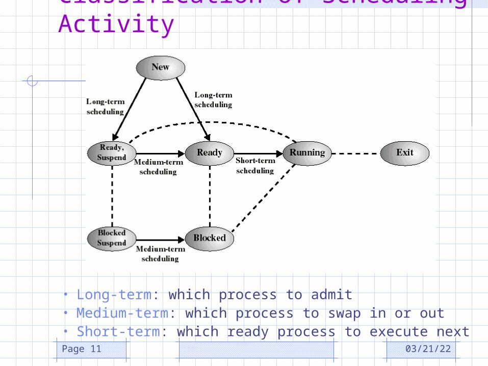
Classification of Scheduling Activity

• Long-term: which process to admit• Medium-term: which process to swap in or out• Short-term: which ready process to execute next

04/18/23Page 12

First-Come, First-Served (FCFS) Scheduling

ProcessBurst TimeP1 24

P2 3

P3 3

• Suppose that the processes arrive in the order: P1 , P2 , P3

The Gantt Chart for the schedule is:

Waiting time for P1 = 0; P2 = 24; P3 = 27• Average waiting time: (0 + 24 + 27)/3 = 17

P1 P2 P3

24 27 300

04/18/23Page 13

FCFS Scheduling (Cont.)Suppose that the processes arrive in the order

P2 , P3 , P1 .• The Gantt chart for the schedule is:

• Waiting time for P1 = 6; P2 = 0; P3 = 3• Average waiting time: (6 + 0 + 3)/3 = 3• Much better than previous case.• Convoy effect short process behind long process

P1P3P2

63 300

04/18/23Page 14

Shortest-Job-First (SJR) Scheduling

• Associate with each process the length of its next CPU burst. Use these lengths to schedule the process with the shortest time.

• Two schemes: – nonpreemptive – once CPU given to the process it

cannot be preempted until completes its CPU burst.– preemptive – if a new process arrives with CPU

burst length less than remaining time of current executing process, preempt. This scheme is know as the Shortest-Remaining-Time-First (SRTF).

• SJF is optimal – gives minimum average waiting time for a given set of processes.

04/18/23Page 15

ProcessArrival TimeBurst TimeP1 0.0 7

P2 2.0 4

P3 4.0 1

P4 5.0 4

• Average waiting time = (0 + 6 + 3 + 7)/4 = 4

Example of Non-Preemptive SJF

P1 P3 P2

73 160

P4

8 12

04/18/23Page 16

Example of Preemptive SJF

ProcessArrival TimeBurst TimeP1 0.0 7

P2 2.0 4

P3 4.0 1

P4 5.0 4

• Average waiting time = (9 + 1 + 0 +2)/4 = 3

P1 P3P2

42 110

P4

5 7

P2 P1

16

04/18/23Page 17

Shortest job first: critique• Possibility of starvation for longer

processes as long as there is a steady supply of shorter processes

• Lack of preemption is not suited in a time sharing environment– CPU bound process gets lower priority (as

it should) but a process doing no I/O could still monopolize the CPU if he is the first one to enter the system

• SJF implicitly incorporates priorities: shortest jobs are given preferences

• The next (preemptive) algorithm penalizes directly longer jobs

04/18/23Page 18

Priority Scheduling

• A priority number (integer) is associated with each process

• The CPU is allocated to the process with the highest priority (smallest integer highest priority).– Preemptive– nonpreemptive

• SJF is a priority scheduling where priority is the predicted next CPU burst time.

• Problem Starvation – low priority processes may never execute.

• Solution Aging – as time progresses increase the priority of the process.

04/18/23Page 19

Round Robin (RR)• Each process gets a small unit of CPU time (time

quantum), usually 10-100 milliseconds. After this time has elapsed, the process is preempted and added to the end of the ready queue.

• If there are n processes in the ready queue and the time quantum is q, then each process gets 1/n of the CPU time in chunks of at most q time units at once. No process waits more than (n-1)q time units.

• Performance– q large FIFO– q small q must be large with respect to context

switch, otherwise overhead is too high.

04/18/23Page 20

Example of RR with Time Quantum = 20

Process Burst TimeP1 53

P2 17

P3 68

P4 24• The Gantt chart is:

• Typically, higher average turnaround than SJF, but better response.

P1 P2 P3 P4 P1 P3 P4 P1 P3 P3

0 20 37 57 77 97 117 121 134 154 162

04/18/23Page 21

Determining Length of Next CPU Burst

• Can only estimate the length.• Can be done by using the length of

previous CPU bursts, using exponential averaging.

:Define 4.

10 , 3.

burst CPU next the for value predicted 2.

burst CPU of lenght actual 1.

1n

thn nt

.1 1 nnn t

04/18/23Page 22

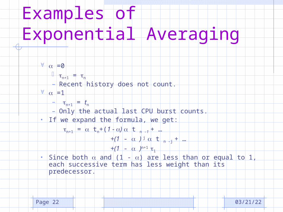
Examples of Exponential Averaging

=0 n+1 = n

– Recent history does not count. =1

– n+1 = tn

– Only the actual last CPU burst counts.• If we expand the formula, we get:

n+1 = tn+(1 - ) t n -1 + …

+(1 - ) j t n -j + …

+(1 - )n+1 1

• Since both and (1 - ) are less than or equal to 1, each successive term has less weight than its predecessor.

04/18/23Page 23

More on Exponential Averaging1. S[n+1] next burst, S[n] current burst

(predicted), T[n] actual,– S[n+1] = T[n] + (1-) S[n] ; 0 < < 1– more weight is put on recent instances

whenever > 1/n2. By expanding this eqn, we see that weights of

past instances are decreasing exponentially– S[n+1] = T[n] + (1-)T[n-1] + ... (1-

)iT[n-i] + ... + (1-)nS[1]– predicted value of 1st instance S[1] is not

calculated; usually set to 0 to give priority to new processes

04/18/23Page 24

Exponentially Decreasing Coefficients

Example

• Assume the following burst-time pattern for a process: 6, 4, 6, 4, 13,13, 13 and assume the initial guess is 10. Predict the next burst-time, α=0.8. Ans: use the equation in item 1. last slide.

04/18/23Page 25

Sn 10 6.8 4.56 5.71 4.34 11.27

12.49

Tn 6 4 6 4 13 13 13

Sn+1 6.8 4.56 5.71 4.34 11.27 12.49 12.89

04/18/23Page 26

Summary• Scheduling is important for improving the

system performance.• Methods of prediction play an important

role in Operating system and network functions.

• Simulation is a way of experimentally evaluating the performance of a technique.

• We will examine queuing theory that allows for modeling of the scheduling disciplines.