6. unconditional logistic regression for … · unconditional logistic regression ... 6.2 general...
TRANSCRIPT
6. UNCONDITIONAL LOGISTIC REGRESSION FOR LARGE STRATA
6.1 Introduction to the logistic model
6.2 General definition of the logistic model
6.3 Adaptation of the logistic model to case-control studies
6.4 Likelihood inference: an outline
6.5 Combining results from 2 x 2 tables
6.6 Qualitative analysis of grouped data from Ille-et-Vilaine
6.7 Quantitative analysis of grouped data
6.8 Regression adjustment for confounders
6.9 Analysis of continuous data
6.10 Interpretation of regression coefficients
6.1 1 Transforming continuous risk variables
6.12 Studies of interaction in a series of 2 x 2 tables
CHAPTER 6
UNCONDITIONAL LOGISTIC REGRESSION FOR LARGE STRATA
The elementary techniques described above for stratified analysis of case-control studies, and in particular the Mantel-Haenszel combined relative risk estimate and test statistic, have served epidemiologists well for over two decades. Most of the cal- culations are simple enough for an investigator to carry out himself, although this often means devoting considerable time to routine chores. Some of the boredom may be alleviated through the use of modern programmable calculators, for which the methods are ideally suited. By working closely with his data, examining them in tabular form, calculating relative risks separately for each stratum, and so on, the researcher can spot trends or inconsistencies he might not otherwise have noticed. Errors in the data may be discovered in this way, and new hypotheses generated.
Nevertheless there are certain limitations inherent in the elementary techniques that must be recognized. If many potentially confounding factors must be controlled simultaneously, a stratified analysis will ultimately break down. Individual strata simply become so large in number and small in size that many of them contain only cases or only controls. This means that substantial amounts of data are effectively lost from the analysis. There are similar limits on the number of categories into which continuous risk factors can be broken down for calculation of separate estimates of relative risk. It is desirable to leave them as continuous variables for purposes of interpolation and extrapolation. The inconsistencies arising from the selection of different levels of a variable to serve as baseline have already been noted, and while often relatively minor, these can be irritating. Limitations are likewise imposed on the extent to which one can analyse the joint effects of several risk factors. Perhaps even more important are the deficiencies in the elementary methods for evaluating interactions among risk and nuisance variables. The usual tests are notoriously lacking in statistical power against patterns of interaction which one might well expect to observe in practice. Other than calculating a separate estimate for each stratum, no provision is made for incorporating such interactions into the estimates of relative risk.
Access to high-speed computing machinery and appropriate statistical software removes these limitations and opens up new possibilities for the statistical analysis of case-control data. By entering a few simple commands into a computer terminal, the investigator can carry out a range of exploratory analyses which could take days or weeks to perform by hand, even with a programmable calculator. He has a great deal of flexibility in choosing how variables are treated in the analysis, how they are cate- gorized, or how they are transformed. The possibilities for multivariate analysis are
LOGISTIC REGRESSION FOR LARGE STRATA 193
virtually limitless. Such methods should, of course, be used in conjunction with tabular presentation of the basic data. Liberal use of charts and graphs to represent the results of the analyses is also recommended.
The basic tool which allows the scope of case-control study analysis to be thus broadened is the linear logistic regression model. Here we introduce the logistic model as a method for multivariate analysis of prospective or cohort studies, which reflects the historical fact that the model was specifically designed for, and first used with, such investigations. Its equal suitability for use in case-control investigations follows as a logical consequence. We replicate the stratified analyses of Chapter 4 using the modelling approach, and then extend these analyses by the inclusion of additional variables so as to illustrate the full power and potential of the method.
Unfortunately the level of statistical sophistication demanded from the reader for full appreciation of the modelling approach is more advanced than it has been in the past. While we have attempted to make the discussion as intelligible as possible for the non-specialist, familiarity with certain aspects of statistical theory, especially linear models and likelihood inference, will undoubtedly facilitate complete understanding.
6.1 Introduction to the logistic model
Whether using the follow-up or case-control approach to study design, cancer epi- demiologists typically collect data on a number of variables which may influence disease risk. Each combination of different levels of these variables defines a category for which an estimate of the probability of disease development is to be made. For example, we way want to determine the risk of lung cancer for a man aged 55 years who has worked 30 years as a telephone linesman and smoked 20 cigarettes per day since his late teens.
If a large enough population were available for study, and if we had unlimited time and money, an obvious approach to this problem would be to collect sufficient numbers of subjects in each category in order to make a precise estimate of risk for each category separately. Of course in the case-control situation these risk estimates would not be absolute, but instead would be relative to that for a designated baseline category. With such a vast amount of data there would be no need to borrow information from neighbouring categories, i.e., those having identical levels for some of the risk variables and similar levels for the remainder, in order to get stable estimates of risk.
Epidemiological studies of cancer, however, rarely even come close to this ideal. Often the greatest limitation is simply the number of cases available for study within a reasonable time period. While this number may be perfectly adequate for assessing the relative risks associated with a few discrete levels of a single risk factor, it is usually insufficient to provide separate estimates for the large number of categories generated by combining even a few more or less continuous factors. Thus we are faced with the problem of having to make smoothed estimates which do utilize information from surrounding categories in order to estimate the risks in each one.
Such smoothing is carried out in terms of a model, which relates disease risk to the various combinations of factor levels which define each risk category via a mathematical formula. The model gives us a simplified, quantitative description of the main features of the relationship between the several risk factors and the probability of disease
194 BRESLOW & DAY
development. It enables us to predict the risk even for categories in which scant infor- mation is available. Important features for the model to have are that it provide mean- ingful results, describe the observed data well and, within these constraints, be as simple as possible. In view of the discussion in Chapter 2, therefore, the parameters of any proposed model should be readily interpretable in terms of relative risk. The model should also allow relative risks corresponding to two or more distinct factors to be represented as the product of individual relative risks, at least as a first approxi- mation.
A model which satisfies these requirements, indeed which has in part been developed specifically to meet them, is the linear logistic model. It derives its name from the fact that the logit transform of the disease probability in each risk category is expressed as a linear function of regression variables whose values correspond to the levels of exposure to the risk factors. In symbols, if P denotes the disease risk, the logit transform y is defined by
y = logit P = log - (1:P)'
or, conversely, expressing P in terms of y,
Since P/(1-P) denotes the disease odds, another name for logit is log odds. Cox (1970) develops the theory of logistic regression in some detail.
The simplest example of logistic regression is provided by the ubiquitous 2 x 2 table considered in 5 2.8 and 5 4.2. Suppose that there is but a single factor and two risk categories, exposed and unexposed, and let PI and Po denote the associated disease probabilities. According to the discussion in 5 2.8 the key parameter, which is both estimable from case-control studies and interpretable as a relative risk, is the odds ratio
Its logarithm, i.e., the log relative risk, may be expressed
p = log II, = logit PI - logit Po
as the diflerence between two logits. Let us define a single binary regression variable x by x = 1 for exposed and x = 0 for unexposed. If we write P(x) for the disease prob- ability associated with an exposure x, and r(x) = P(x)Qo/PoQ(x) for the relative risk (odds ratio relative to x = 0), we have
log r(x) = px
where a = logit Po. There is a perfect correspondence between the two parameters a andp in the mod'el and the two disease risks such that
LOGISTIC REGRESSION FOR LARGE STRATA
and
The formulation (6.3) focuses on the key parameter, P, and suggests how to extend the model for more complex problems.
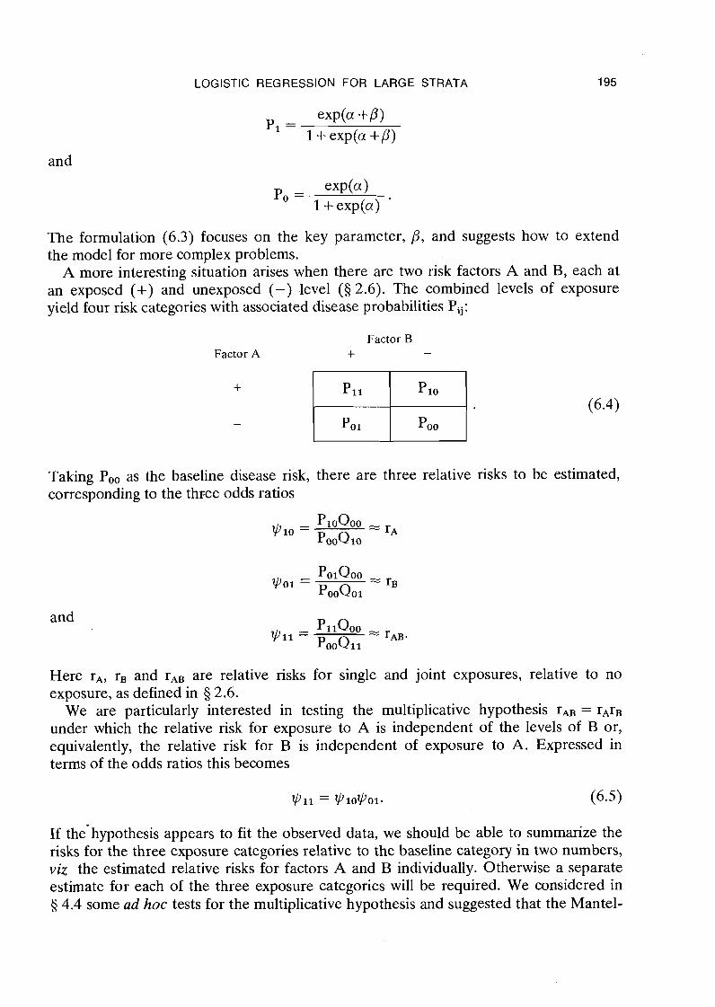
A more interesting situation arises when there are two risk factors A and B, each at an exposed (+) and unexposed (-) level ( 5 2.6). The combined levels of exposure yield four risk categories with associated disease probabilities Pij:
Factor B Factor A + -
Taking Po, as the baseline disease risk, there are three relative risks to be estimated, corresponding to the t h ~ e e odds ratios
and
Here rA, rB and rAB are relative risks for single and joint exposures, relative to no exposure, as defined in 5 2.6.
We are particularly interested in testing the multiplicative hypothesis TAB = rArB under which the relative risk for exposure to A is independent of the levels of B or, equivalently, the relative risk for B is independent of exposure to A. Expressed in terms of the odds ratios this becomes
lyll = lyl0ly01. (6.5)
If the-hypothesis appears to fit the observed data, we should be able to summarize the risks for the three exposure categories relative to the baseline category in two numbers, viz the estimated relative risks for factors A and B individually. Otherwise a separate estimate for each of the three exposure categories will be required. We considered in 5 4.4 some ad hoc tests for the multiplicative hypothesis and suggested that the Mantel-
196 BRESLOW & DAY
Haenszel formula be used to estimate the individual relative risks if the hypothesis were accepted.
Estimates and tests of the multiplicative hypothesis are simply obtained in terms of a logistic regression model for the disease probabilities (6.4). Define the binary regres- sion variable xl = 1 or 0 according to whether a person is exposed to Factor A or not, and similarly let x2 indicate the levels of exposure to Factor B. Variables such as xl and x2, which take on 0-1 values only, are sometimes called dummy or indicator variables since they serve to identify different levels, of exposure rather than expressing it in quantitative terms. Note that the product xlx2 equals 1 only for the double exposure category. Let us define P(xl,x2) as the disease probability, and r(xl,x2) as the relative risk (odds ratio) relative to the unexposed category xl = x2 = 0. Then we can re-express the relative risks, or equivalently the probabilities, using the model
Since there are four parameters a,Pl,P2 and y to describe the four probabilities Pij, we say that the model is completely saturated. It imposes n o constraints whatsoever on the relationships between the four probabilities or the corresponding odds ratios. Thus we may solve equation (6.6) explicitly for the four parameters, obtaining
as the logit transform of the baseline disease probability,
and
as the log relative risks for individual exposures, and
as the interaction parameter. It is clear from (6.7) that exp(y) represents the multi- plicative factor by which the relative risk for the double exposure category differs from the product of relative risks for the individual exposures. If y > 0, a positive inter- action, the risk accompanying the combined exposure is greater than predicted by the individual effects; if y < 0, a negative interaction, the combined risk is less. Testing the multiplicative hypothesis (6.5) is equivalent to testing that the interaction param- eter y in the logistic model is equal to 0.
If the hypothesis y = 0 is accepted by our test criterion, we would consider fitting to the data the reduced three parameter model
LOGISTIC REGRESSION FOR LARGE STRATA 197
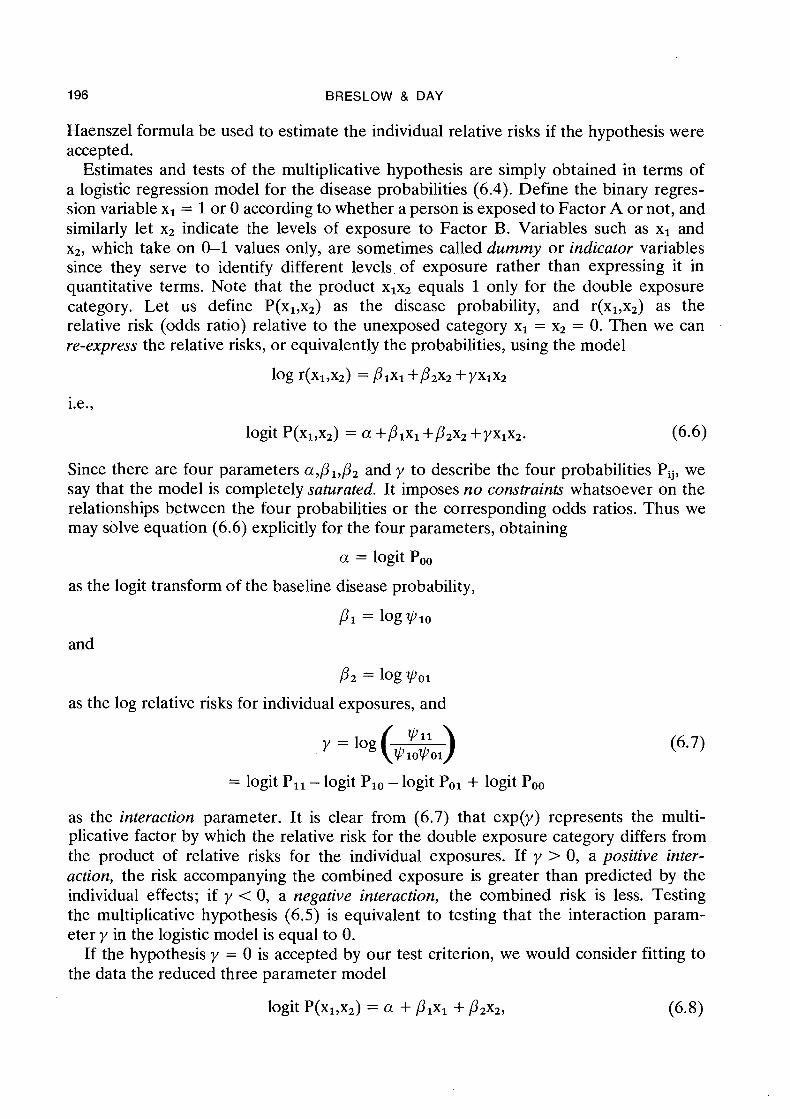
which re-expresses the multiplicative hypothesis in logit terms. This model does impose constraints on the four disease probabilities Pij. For example, since
v 11 P I = logvlo = log- v01
now represents the log relative risk for A whether or not exposure to B occurs, it would be estimated by combining information from the 2 x 2 tables
Cases
Controls
Factor B + Factor A
Factor B - Factor A
Odds ratio ~ I I / ~ ~ O I v 10
Likewise the estimate of
4'11 P z = log V0l = log
would combine information from both the tables
Factor A + Factor B
Factor A - Factor B
Cases
Controls
Odds ratio
The difference between the interpretation of PI in (6.6) and the same parameter in (6.8) illustrates that the meaning of the regression coefficients in a model depends on what other variables are included. In the saturated model PI represents the log relative risk for A at level 0 of B only, whereas in (6.8) it represents the log relative risk for A at both levels of B. Testing the hypothesis PI = 0 in (6.8) is equivalent to testing the hypothesis that Factor A has no effect on risk, against the alternative hypo- thesis that there is an effect, but one which does not depend on B. It makes little. sense to test pl = 0 in (6.6), or more generally to test for main effects being zero in the presence of interactions involving the same factors. Models which contain interaction terms without the corresponding main effects correspond to hypotheses of no practical interest (Nelder, 1977).
The regression approach is easily generalized to incorporate the effects of more than
198 BRESLOW & DAY
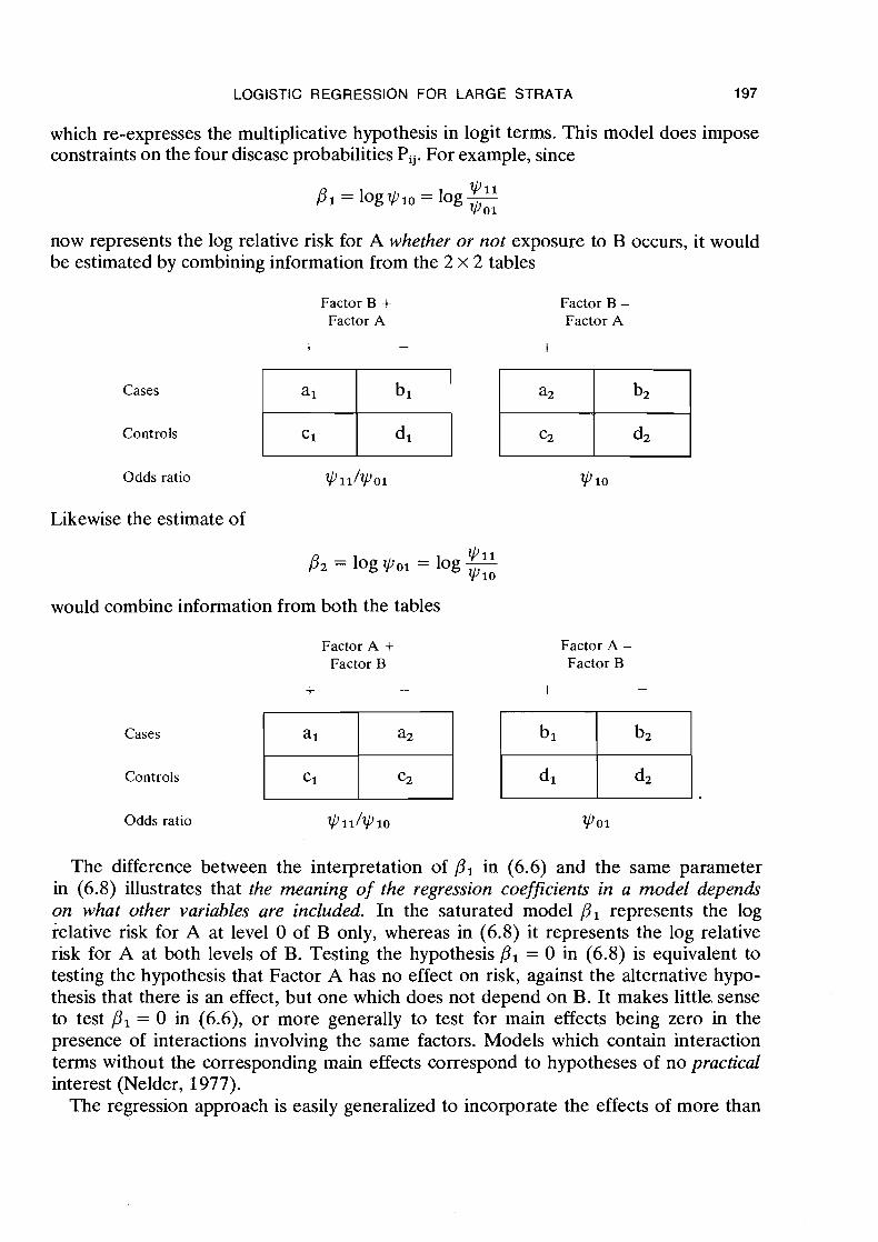
two risk factors, or risk factors at more than two levels. Suppose that Factor B occurred at three levels, say 0 = low, 1 = medium and 2 = high. There would then be six disease probabilities
Factor A
Exposed
Unexposed
and five odds ratios
Factor B
High Medium Low
Pij QOO Vij =
POO Qij '
where all risks are expressed relative to Poo as baseline. In order to identify the three levels of Factor B, two indicator variables x2 and x3 are required in place of the single x2 used earlier. These are coded as follows:
Factor B
High Medium Low
More generally, for a factor with K levels, K-1 indicator variables will be needed to describe its effects. With xl defining exposure to A as before, the saturated model with six parameters is written
where the values of the x's are determined from the factor levels i and j. Now the multiplicative hypothesis
corresponds to setting both interaction parameters y12 and yl3 to zero, in which case the coefficients p2 and p3 represent the log relative risks for levels 1 and 2 of Factor B as compared with level 0.
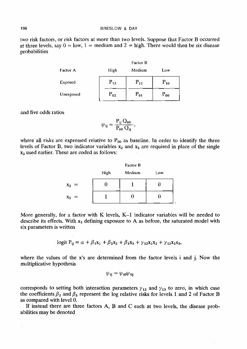
If instead there are three factors A, B and C each at two levels, the disease prob- abilities may be denoted
LOGISTIC REGRESSION FOR LARGE STRATA
Factor A
+
-
Factor C + Factor B
Factor C - Factor B
+ -
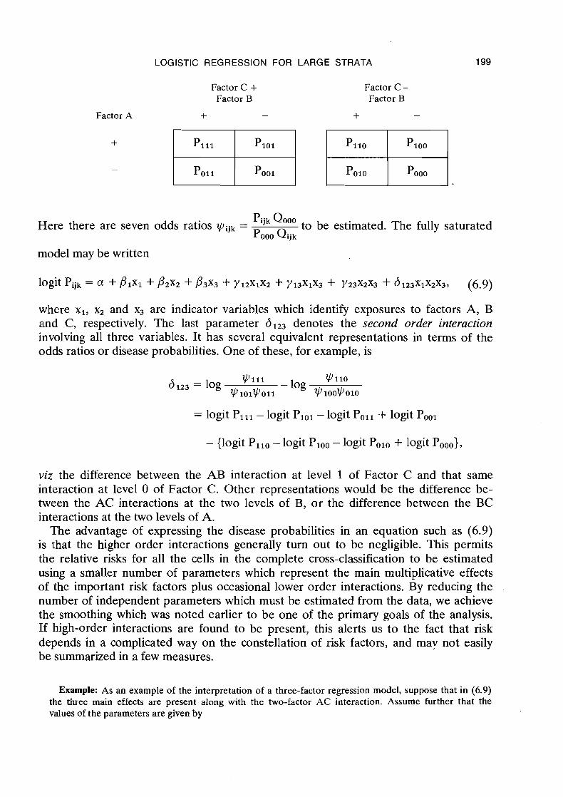
Here there are seven odds ratios vijk = QOoo to be estimated. The fully saturated POOO Qijk
model may be written
where xl, x2 and x3 are indicator variables which identify exposures to factors A, B and C, respectively. The last parameter d123 denotes the second order interaction involving all three variables. It has several equivalent representations in terms of the odds ratios or disease probabilities. One of these, for example, is
v111 4'110 6 123 = log - log
v101v011 v1oovo10
= logit Pill - logit PIOl - logit Poll + logit Pool
- {logit Pllo - logit Ploo - logit Polo + logit Pooo),
viz the difference between the AB interaction at level 1 of Factor C and that same interaction at level 0 of Factor C. Other representations would be the difference be- tween the AC interactions at the two levels of B, or the difference between the BC interactions at the two levels of A.
The advantage of expressing the disease probabilities in an equation such as (6.9) is that the higher order interactions generally turn out to be negligible. This permits the relative risks for all the cells in the complete cross-classification to be estimated using a smaller number of parameters which represent .the main multiplicative effects of the important risk factors plus occasional lower order interactions. By reducing the number of independent parameters which must be estimated from the data, we achieve the smoothing which was noted earlier to be one of the primary goals of the analysis. If high-order interactions are found to be present, this alerts us to the fact that risk depends in a complicated way on the constellation of risk factors, and mav not easily be summarized in a few measures.
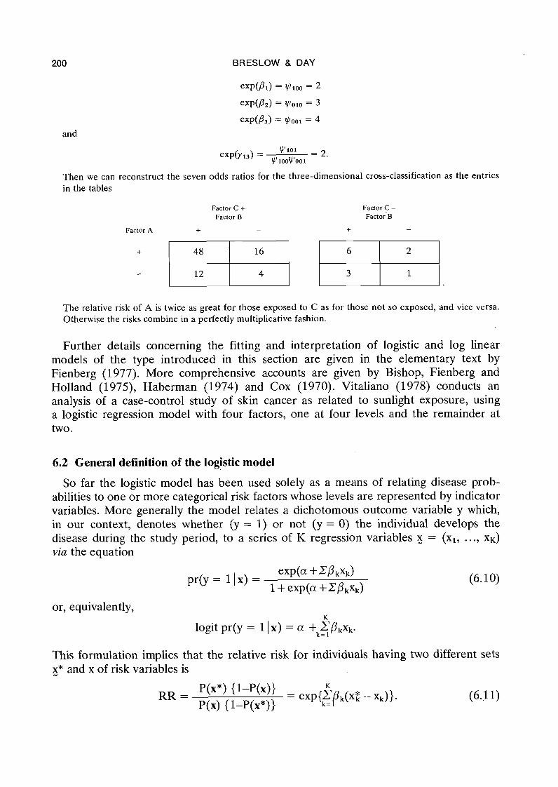
Example: As an example of the interpretation of a three-factor regression model, suppose that in (6.9) the three main effects are present along with the two-factor AC interaction. Assume further that the values of the parameters are given by
BRESLOW & DAY
and
Then we can reconstruct the seven odds ratios for the three-dimensional cross-classification as the entries in the tables
Factor C + Factor B
Factor C - Factor B
Factor A + - + -
The relative risk of A is twice as great for those exposed to C as for those not so exposed, and vice versa. Otherwise the risks combine in a perfectly multiplicative fashion.
Further details concerning the fitting and interpretation of logistic and log linear models of the type introduced in this section are given in the elementary text by Fienberg (1977). More comprehensive accounts are given by Bishop, Fienberg and Holland (1975), Haberman (1974) and Cox (1970). Vitaliano (1978) conducts an analysis of a case-control study of skin cancer as related to sunlight exposure, using a logistic regression model with four factors, one at four levels and the remainder at two.
6.2 General definition of the logistic model
So far the logistic model has been used solely as a means of relating disease prob- abilities to one or more categorical risk factors whose levels are represented by indicator variables. More generally the model relates a dichotomous outcome variable y which, in our context, denotes whether (y = 1) or not (y = 0) the individual develops the disease during the study period, to a series of K regression variables = (xl, ..., xK) via the equation
or, equivalently, K
logit pr(y = 11 x) = a + k= EPkxk. I
This formulation implies that the relative risk for individuals having two different sets x* and x of risk variables is
LOGISTIC REGRESSION FOR LARGE STRATA 201
Thus a represents the log odds of disease risk for a person with a standard (x = 0) set of regression variables, while exp(P,) is the fraction by which this risk is increased (or decreased) for every unit change in x,. A large number of possible relationships may be represented in this form by including among the x's indicator variables and continuous measurements, transformations of such measurements, and cross-product or interaction variables.
As we saw in the last chapter, one important means of controlling the effects of nuisance or confounding variables is by stratification of the study population on the basis of combinations of levels of these variables. When conducting similar analyses in the context of logistic regression, it is convenient to generalize the model further so as to isolate the stratum effects, which are often of little intrinsic interest, from the effects of the risk factors under study. With Pi(x) denoting the disease probability in-stratum i for an individual with risk variables x, we may write
If .none of the regression variables are interaction terms involving the factors used for stratification, a consequence of (6.12) is that the relative risks associated with the risk factors under study are constant over strata. By including such interaction terms among the x's, one may model changes .in the relative risk which accompany changes in the stratification variables. The fact that the parameters of the logistic model are so easily interpretable in terms of relative risk is, as we have said, one of the main reasons for using the model.
The earliest applications of this model were in prospective studies of coronary heart disease in which x represented such risk factors as age, blood pressure, serum cholesterol and cigarette consumption (Cornfield, 1962; Truett, Cornfield & Kannel, 1967). In these investigations the authors used linear discriminant analysis to estimate the param- eters, an approach which is strictly valid only if the x's have multivariate normal distributions among both diseased and non-diseased (see 5 6.3). The generality of the method was enhanced considerably by the introduction of maximum likelihood estima- tion procedures (Walker & Duncan, 1967; Day & Kerridge, 1967; Cox, 1970). These are now available in several computer packages, including the General Linear Inter- active Modelling system (GLIM) distributed by the Royal Statistical Society (Baker & Nelder, 1978).
We noted in 5 2.8 that for a long st.udy it is appropriate to partition the time axis into several intervals and use these .as one of the criteria for forming strata. In the present context this means that the quantity Pi(x) refers more specifically to the conditional probability of developing disease during the time interval specified by the ith stratum, given that the subject was disease-free at its start. For follow-up or cohort studies, if we are to use conventional computer programmes for logistic regression with conditional probabilities, separate data records must be read into the computer for each stratum in which an individual appears. Thomson (1977) discusses in some detail the problems of estimation in this situation.
A limiting form of the logistic model for conditional probabilities, obtained by allow- ing the time intervals used for stratification to become infinitesimally small, is known as the proportional hazards model (Cox, 1972). Here the ratio of incidence rates for
202 BRESLOW & DAY
individuals with exposures x* and x is given exactly by the right-hand side of equation (6.11). This approach has the conceptual advantage of eliminating the odds ratio approximation altogether, and thus obviates the rare disease assumptipn. The model has a history of successful use in .the statistical analysis of survival studies, and it is becoming increasingly clear that many of the analytic techniques developed for use in that field can also be applied in epidemiology (Breslow, 1975, 1978). Prentice and Breslow (1978) present a detailed mathematical treatment of the role of the propor- tional hazards model in the analysis of case-control study data. Methodological tech- niques stemming from the model are identical to those presented in Chapter 7 on matched data.
6.3 Adaptation of the logistic model to case-control studies1
According to the logistic model as just defined, the exposures x are regarded as fixed quantities while the response variable y is random. This fits precisely the cohort study situation because it is not known in advance whether or not, or when, a given individual will develop the disease. With the case-control approach, QII the other hand, subjects are selected on the basis of their disease status. It is their history of risk factor exposures, as determined by retrospective interview or other means, which should properly be regarded as the random outcome. Thus an important question, addressed in this section, is: how can the logistic model for disease probabilities, which has such a simple and desirable interpretation vis-a-vis relative risk, be adapted for use with a sample of cases and controls?
If there is but a single binary risk factor with study subjects classified simply as ex- posed versus unexposed, the answer to this is perfectly clear. Recall first of all our demonstration in 5 2.8 that the odds ratio q of disease probabilities for exposed versus unexposed is identical to the odds ratio of exposure probabilities for diseased versus disease-free. When drawing inferences about on the basis of data in 2 x 2 tables (4.1), it makes absolutely no difference whether the marginal totals ml and mo cor- responding to the two exposure categories are fixed, as in a cohort study, or whether the margins nl and no of diseased and disease-free are fixed, as in a case-control study. The estimates, tests and confidence intervals for q derived in 5 4.1 and 5 4.2 in no way depend on how the data in the tables are obtained. Hence we have already de- monstrated for 2 x 2 tables that inferences about relative risk are made by applying to case-control data precisely the same set of calculations as would be applied to cohort data from the same population.
This identity of inferential procedures, whether sampling is carried out according to a cohort or case-control design, is in fact a fundamental property of the general logistic model. We illustrate this feature with a simple calculation involving conditional prob- abilities (Mantel, 1973; Seigel & Greenhouse, 1973) which lends a good deal of plau- sibility to the deeper mathematical results discussed afterwards. It suffices to consider the model (6.10) for disease probabilities in a single population, as results for the
'This section, which is particularly abstract, deals with the logical basis for the application of logistic regression to case-control data. Readers interested only in practical applications can go directly to 5 6.5.
LOGISTIC REGRESSION FOR LARGE STRATA 203
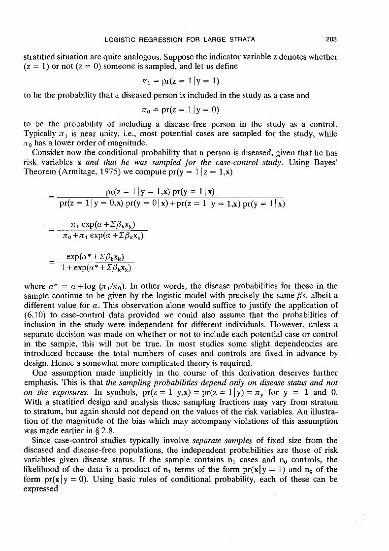
stratified situation are quite analogous. Suppose the indicator variable z denotes whether (z = 1) or not (z = 0) someone is sampled, and let us define
to be the probability that a diseased person is included in the study as a case and
to be the probability of including a disease-free person in the study as a control. Typically x1 is near unity, i.e., most potential cases are sampled for the study, while xo has a lower order of magnitude.
Consider now the conditional probability that a person is diseased, given that he has risk variables x and that he was sampled for the case-control study. Using Bayes' Theorem (Armitage, 1975) we compute pr(y = 1 1 z = 1,x)
where a* = u +log ( J Z ~ / X ~ ) . In other words, the disease probabilities for those in the sample continue to be given by the logistic model with precisely the same ps, albeit a different value for a. This observation alone would suffice to justify the application of (6.10) to case-control data provided we could also assume that the probabilities of inclusion in the study were independent for different individuals. However, unless a separate decision was made on whether or not to include each potential case or control in the sample, this will not be true. In most studies some slight dependencies are introduced because the total numbers of cases and controls are fixed in advance by design. Hence a somewhat more complicated theory is required.
One assumption made implicitly in the course of this derivation deserves further emphasis. This is that the sampling probabilities depend only on disease status and not on the exposures. In symbols, pr(z = 1 1 y,x) = pr(z = 1 1 y) = n, for y = 1 and 0. With a stratified design and analysis these sampling fractions may vary from stratum to stratum, but again should not depend on the values of the risk variables. An illustra- tion of the magnitude of the bias which may accompany violations of this assumption was made earlier in 5 2.8.
Since case-control studies typically involve separate samples of fixed size from the diseased and disease-free populations, the independent probabilities are those of risk variables given disease status. If the sample contains nl cases and no controls, the likelihood of the data is a product of nl terms of the form pr(x1 y = 1) and no of the form pr(x1 y = 0). Using basic rules of conditional probability, each of these can be expressed
204 BRESLOW & DAY
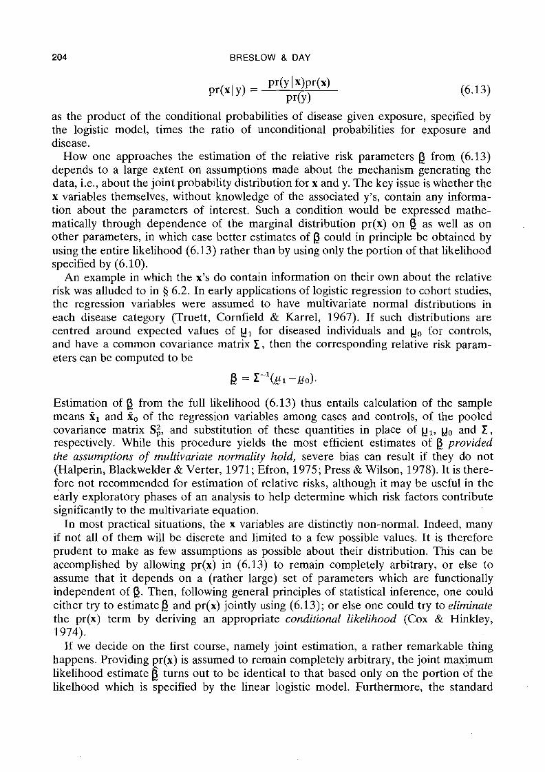
as the product of the conditional probabilities of disease given exposure, specified by the logistic model, times the ratio of unconditional probabilities for exposure and disease.
How one approaches the estimation of the relative risk parameters P from (6.13) depends to a large extent on assumptions made about the mechanism generating the data, i.e., about the joint probability distribution for x and y. The key issue is whether the x variables themselves, without knowledge of the associated y's, contain any informa- tion about the parameters of interest. Such a condition would be expressed mathe- matically through dependence of the marginal distribution pr(x) on & as well as on other parameters, in which case better estimates of P could in principle be obtained by using the entire likelihood (6.13) rather than by using only the portion of that likelihood specified by (6.10).
An example in which the x's do contain information on their own about the relative risk was alluded to in tj 6.2. In early applications of logistic regression to cohort studies, the regression variables were assumed to have multivariate normal distributions in each disease category (Truett, Cornfield & Karrel, 1967). If such distributions are centred around expected values of g1 for diseased individuals and p0 for controls, and have a common covariance matrix 1, then the corresponding r e l a h e risk param- eters can be computed to be
Estimation of from the full likelihood (6.13) thus entails calculation of the sample means x1 and xo of the regression variables among cases and controls, of the pooled covariance matrix Sg, and substitution of these quantities in place of bl, uo and 1 , respectively. While this procedure yields the most efficient estimates of f.3 - provided the assumptions of multivariate normality hold, severe bias can result if they do not (Halperin, Blackwelder & Verter, 1971; Efron, 1975; Press & Wilson, 1978). It is there- fore not recommended for estimation of relative risks, although it may be useful in the early exploratory phases of an analysis to help determine which risk factors contribute significantly to the multivariate equation.
In most practical situations, the x variables are distinctly non-normal. Indeed, many if not all of them will be discrete and limited to a few possible values. It is therefore prudent to make as few assumptions as possible about their distribution. This can be accomplished by allowing pr(x) in (6.13) to remain completely arbitrary, or else to assume that it depends on a (rather large) set of parameters which are functionally independent of &. Then, following general principles of statistical inference, one could either try to estimate and pr(x) jointly using (6.13); or else one could try to eliminate the pr(x) term by deriving an appropriate conditional likelihood (Cox & Hinkley, 1974).
If we decide on the first course, namely joint estimation, a rather remarkable thing happens. Providing pr(x) is assumed to remain completely arbitrary, the joint maximum likelihood estimate turns out to be identical to that based only on the portion of the likelhood which is specified by the linear logistic model. Furthermore, the standard
LOGISPIC REGRESSION FOR LARGE STRATA 205
errors and covariances for generated from partial and full likelihoods also agree. This fact was first noted by Anderson (1972) for the case in which x was a discrete variable, and established for the general situation by Prentice and Pyke (1979).
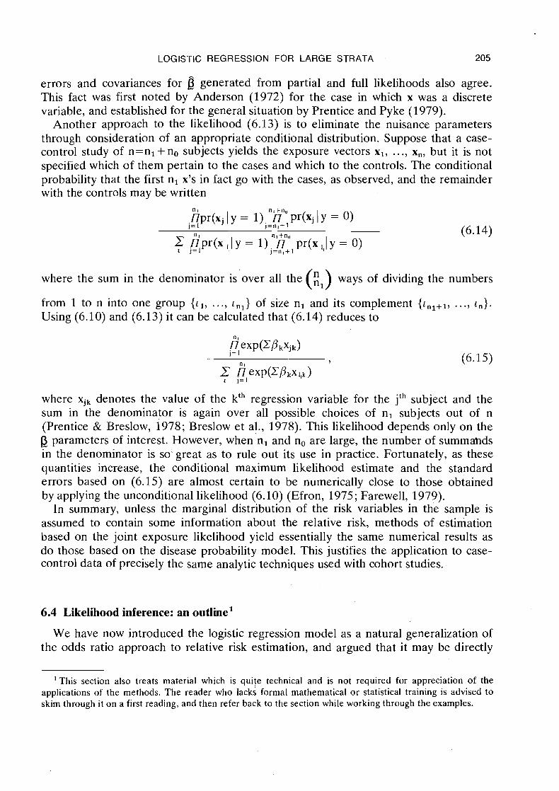
Another approach to the likelihood (6.13) is to eliminate the nuisance parameters through consideration of an appropriate conditional distribution. Suppose that a case- control study of n=n, +no subjects yields the exposure vectors x,, ..., x,, but it is not specified which of them pertain to the cases and which to the controls. The conditional probability that the first n, x's in fact go with the cases, as observed, and the remainder with the controls may be written
where the sum in the denominator is over all the (:,) ways of dividing the numbers
from 1 to n into one group {I,, .. ., I,,) of size n, and its complement {I,,,~, . . ., 1 , ) .
Using (6.10) and (6.13) it can be calculated that (6.14) reduces to
where xjk denotes the value of the kth regression variable for the jth subject and the sum in the denominator is again over all possible choices of n, subjects out of n (Prentice & Breslow, 1978; Breslow et al., 1978). This likelihood depends only on the p parameters of interest. However, when n, and no are large, the number of s u m m a ~ d s rn the denominator is so' great as to rule out its use in practice. Fortunately, as these quantities increase, the conditional maximum likelihood estimate and the standard errors based on (6.15) are almost certain to be numerically close to those obtained by applying the unconditional likelihood (6.10) (Efron, 1975; Farewell, 1979).
In summary, unless the marginal distribution of the risk variables in the sample is assumed to contain some information about the relative risk, methods of estimation based on the joint exposure likelihood yield essentially the same numerical results as do those based on the disease probability model. This justifies the application to case- control data of precisely the same analytic techniques used with cohort studies.
6.4 Likelihood inference: an outline'
We have now introduced the logistic regression model as a natural generalization of the odds ratio approach to relative risk estimation, and argued that it may be directly
'This section also treats material which is quite technical and is not required for appreciation of the applications of the methods. The reader who lacks formal mathematical o r statistical training is advised to skim through it o n a first reading, and then refer back to the section while working through the examples.
206 BRESLOW & DAY
applied to case-control study data with disease status (case versus control) treated as the "dependent" or response variable. Subsequent sections of this chapter will illus- trate its application to several problems of varying complexity. With one exception, the illustrative analyses may all be carried out using standard computer programmes for the fitting of linear logistic models by maximum likelihood.
Input to GLIM or other standard programmes is in the form of a rectangular data array, consisting of a list of values on a fixed number of variables for each subject in the study, with different subjects on different rows. The variables are typically in the order (y,xl, . .., xK), where y equals 1 or 0 according to whether the subject is a case or control, while the x's represent various discrete and/or continuous regression variables to be related to y. Output usually consists of estimates of the regression coefficients for each variable, a variance/covariance matrix for the estimated coefficients, and one or more test statistics which measure the goodness of fit of the model to the observed data. It is not necessary to have a detailed understanding of the arithmetical operations linking the inputs to the outputs in order to be able to use the programme. Researchers in many fields have long used similar programmes for ordinary (least squares) fitting of multiple regression equations, with considerable success. Nevertheless, some apprecia- tion of the fundamental concepts involved can help to dispel the uneasiness which accompanies what otherwise might seem a rather "black box" approach to data analysis. In this section we outline briefly the key features of likelihood inference in the hopes that it may lay the logical foundation for the interpretation of the outputs. More detailed expositions of this material can be found in the books by Cox (1970), Haber- man (1974), Bishop, Fienberg and Holland (1975) and Fienberg (1977).
Statistical inference starts with an expression for the probability, or likelihood, of the observed data. This depends on a number of unknown parameters which represent quantitative features of the population from which the data are sampled. In our situa- tion the likelihood is composed of a product of terms of the form (6.10), one for each subject. The a's and P's are the unknown parameters, inte;est being focused on the P's because of their ready interpretation vis-ci-vis relative risk.
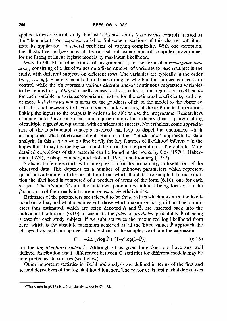
Estimates of the parameters are selected to be those values which maximize the likeli- hood or rather, and what is equivalent, those which maximize its logarithm. The param- eters thus estimated, which are often denoted a and p, are inserted back into the individual likelihoods (6.10) to calculate the fitted or predicted probability P of being a case for each study subject. If we subtract twice the maximized log likelihood from zero, which is the absolute maximum achieved as all the'fitted values P approach the observed y's, and sum up over all individuals in the sample, we obtain the expression
G = -= {ylog P + (l-y)log(l-~)}
for the log likelihood statistic1. Although G as given here does not have any well defined distribution itself, differences between G statistics for different models may be interpreted as chi-squares (see below).
Other important statistics in likelihood analysis are defined in terms of the first and second derivatives of the log likelihood function. The vector of its first partial derivatives
'The statistic (6.16) is called the deviance in GLIM.
LOGISTIC REGRESSION FOR LARGE STRATA 207
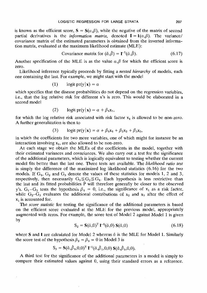
is known as the efficient score, S = S(a,P), while the negative of the matrix of second partial derivatives is the information matrix, denoted I = I(a,P). The variance/ covariance matrix of the estimated parameters is obtained from the inverted informa- tion matrix, evaluated at the maximum likelihood estimate (MLE):
Covariance matrix for (6,)) = I-'(& ,)). (6.17)
Another specification of the MLE is as the value a , p for which the efficient score is zero.
Likelihood inference typically proceeds by fitting a nested hierarchy of models, each one containing the last. For example, we might start with the model
(1) logit pr(y ( x) = a
which specifies that the disease probabilities do not depend on the regression variables, i.e., that the log relative risk for different x's is zero. This would be elaborated in a second model
for which the log relative risk associated with risk factor x1 is allowed to be non-zero. A further generalization is then to
in which the coefficients for two more variables, one of which might for instance be an -
interaction involving xl, are also allowed to be non-zero. At each stage we obtain the MLEs of the coefficients in the model, together with
their estimated variances and covariances. We also carry out a test for the significance of the additional parameters, which is logically equivalent to testing whether the current model fits better than the last one. Three tests are available. The likelihood ratio test is simply the difference of the maximized log likelihood statistics (6.16) for the two models. If GI, G2 and G3 denote the values of these statistics for models 1, 2 and 3, respectively, then necessarily G3 5 G2 5 GI. Each hypothesis is less restrictive than the last and its fitted probabilities P will therefore generally be closer to the observed y's. GI-G2 tests the hypothesis P1 = 0, i.e., the significance of x1 as a risk factor, while G2-G3 evaluates the additional contributions of x, and x3 after the effect of x1 is accounted for.
The score statistic for testing the significance of the additional parameters is based on the efficient score evaluated at the MLE for the previous model, appropriately augmented with zeros. For example, the score test of ~ o d e l 2 against Model 1 is given by
S2 = S(&,O)T I-l(&,O) S(&,O) (6.18)
where S and I are calculated for Model 2 whereas 6 is the MLE for Model 1. Similarly the score test of the hypothesis P2 = P3 = 0 in Model 3 is
A third test for the significance of the additional parameters in a model is simply to compare their estimated values against 0, using their standard errors as a reference.
208 BRESLOW & DAY
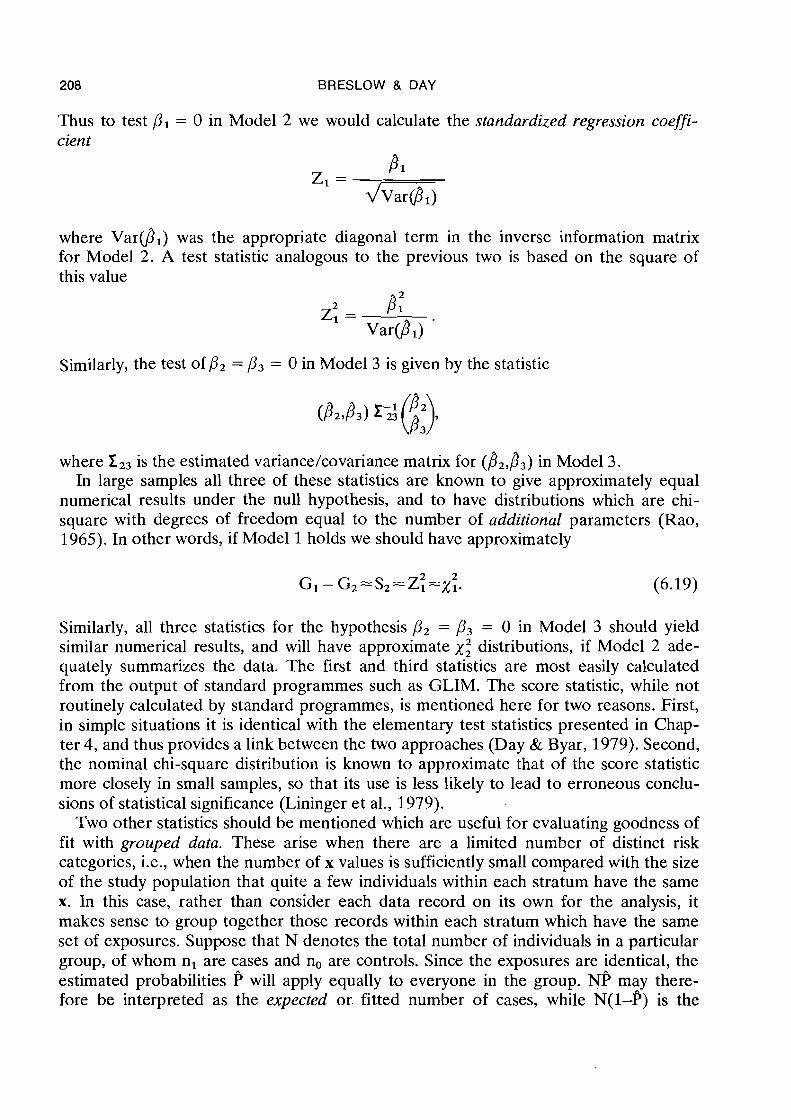
Thus to test P1 = 0 in Model 2 we would calculate the standardized regression coeffi- cient
where var(8,) was the appropriate diagonal term in the inverse information matrix for Model 2. A test statistic analogous to the previous two is based on the square of this value
n 2
Similarly, the test of P2 = P3 = 0 in Model 3 is given by the statistic
where is the estimated variance/covariance matrix for (P2,B3) in Model 3. In large samples all three of these statistics are known to give approximately equal
numerical results under the null hypothesis, and to have distributions which are chi- square with degrees of freedom equal to the number of additional parameters (Rao, 1965). In other words, if Model 1 holds we should have approximately
Similarly, all three statistics for the hypothesis p2 = P3 = 0 in Model 3 should yield similar numerical results, and will have approximate x,2 distributions, if Model 2 ade- quately summarizes the data. The first and third statistics are most easily calculated from the output of standard programmes such as GLIM. The score statistic, while not routinely calculated by standard programmes, is mentioned here for two reasons. First, in simple situations it is identical with the elementary test statistics presented in Chap- ter 4, and thus provides a link between the two approaches (Day & Byar, 1979). Second, the nominal chi-square distribution is known to approximate that of the score statistic more closely in small samples, so that its use is less likely to lead to erroneous conclu- sions of statistical significance (Lininger et al., 1979).
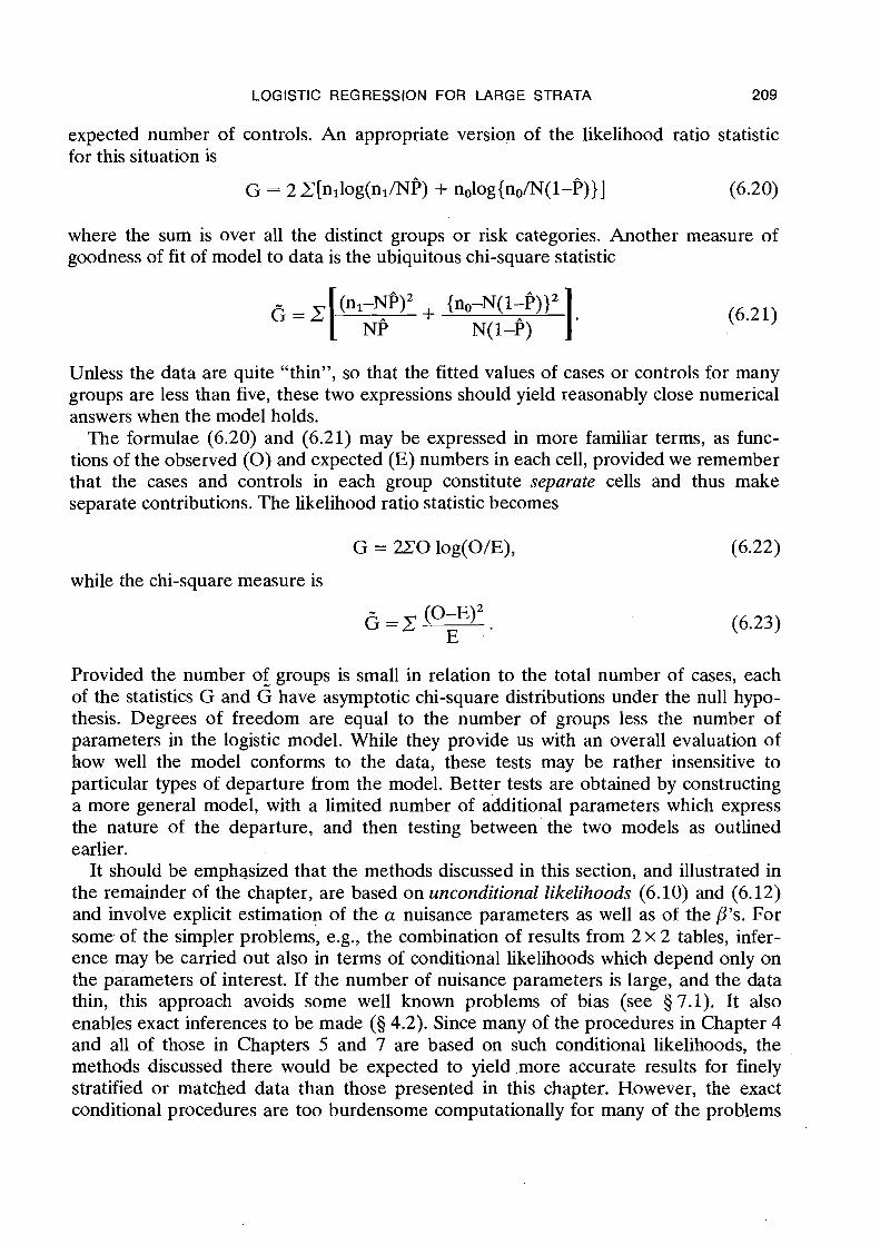
Two other statistics should be mentioned which are useful for evaluating goodness of fit with grouped data. These arise when there are a limited number of distinct risk categories, i.e., when the number of x values is sufficiently small compared with the size of the study population that quite a few individuals within each stratum have the same x. In this case, rather than consider each data record on its own for the analysis, it makes sense to group together those records within each stratum which have the same set of exposures. Suppose that N denotes the total number of individuals in a particular group, of whom nl are cases and no are controls. Since the exposures are identical, the estimated probabilities P will apply equally to everyone in the group. NP may there- fore be interpreted as the expected or fitted number of cases, while ~ ( 1 - p ) is the
LOGISTIC REGRESSION FOR LARGE STRATA 209
expected number of controls. An appropriate version of the likelihood ratio statistic for this situation is
G = 2 C[nl1og(nl/NP) + nolog{no/N(l-P)}] (6.20)
where the sum is over all the distinct groups or risk categories. Another measure of goodness of fit of model to data is the ubiquitous chi-square statistic
Unless the data are quite "thin", so that the fitted values of cases or controls for many groups are less than five, these two expressions should yield reasonably close numerical answers when the model holds.
The formulae (6.20) and (6.21) may be expressed in more familiar terms, as func- tions of the observed ( 0 ) and expected (E) numbers in each cell, provided we remember that the cases and controls in each group constitute separate cells and thus make separate contributions. The likelihood ratio statistic becomes
while the chi-square measure is
Provided the number of groups is small in relation to the total number of cases, each of the statistics G and 6 have asymptotic chi-square distributions under the null hypo- thesis. Degrees of freedom are equal to the number of groups less the number of parameters in the logistic model. While they provide us with an overall evaluation of how well the model conforms to the data, these tests may be rather insensitive to particular types of departure from the model. Better tests are obtained by constructing a more general model, with a limited number of additional parameters which express the nature of the departure, and then testing between'the two models as outlined earlier.
It should be emphasized that the methods discussed in this section, and illustrated in the remainder of the chapter, are based on unconditional likelihoods (6.10) and (6.12) and involve explicit estimation of the a nuisance parameters as well as of the P's. For some. of the simpler problems, e.g., the combination of results from 2 x 2 tables, infer- ence may be carried out also in terms of conditional likelihoods which depend only on the parameters of interest. If the number of nuisance parameters is large, and the data thin, this approach avoids some well known problems of bias (see 5 7.1). It also enables exact inferences to be made (5 4.2). Since many of the procedures in Chapter 4 and all of those in Chapters 5 and 7 are based on such conditional likelihoods, the methods discussed there would be expected to yield more accurate results for finely stratified or matched data than those presented in this chapter. However, the exact conditional procedures are too burdensome computationally for many of the problems
210 BRESLOW & DAY
which confront us. Thus, while we may lose some accuracy with the logistic regression approach, what we gain in return is a coherent methodology capable of handling a wide variety of problems in a uniform manner.
6.5 Combining results from 2 x 2 tables
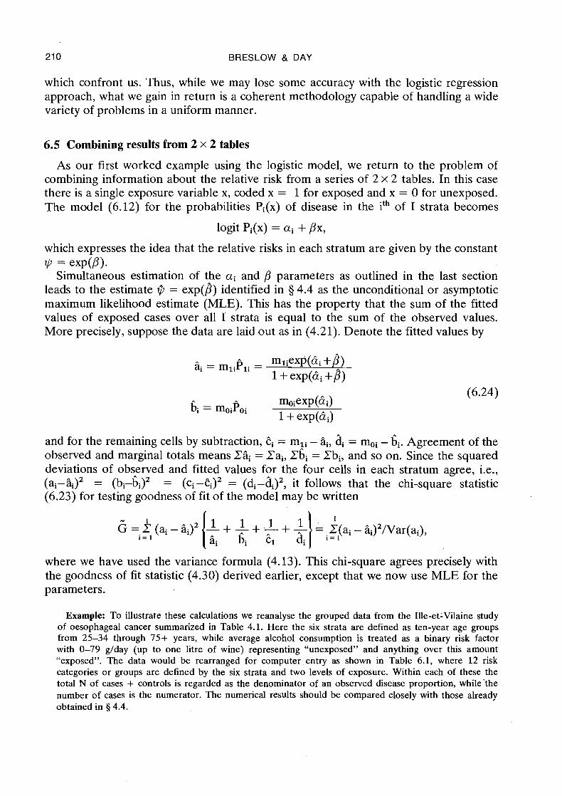
As our first worked example using the logistic model, we return to the problem of combining information about the relative risk from a series of 2 x 2 tables. In this case there is a single exposure variable x, coded x = 1 for exposed and x = 0 for unexposed. The model (6.12) for the probabilities Pi(x) of disease in the ith of I strata becomes
which expresses the idea that the relative risks in each stratum are given by the constant * = = X P ( ~ ) * Simultaneous estimation of the ai and ,Ll parameters as outlined in the last section
leads to the estimate $?J = exp(?) identified in § 4.4 as the unconditional or asymptotic maximum likelihood estimate (MLE). This has the property that the sum of the fitted values of exposed cases over all I strata is equal to the sum of the observed values. More precisely, suppose the data are laid out as in (4.21). Denote the fitted values by
and for the remaining cells by subtraction, ti = mIi - $, di = moi - bi. Agreement of the observed and marginal totals means Eli = Pai7 Pbi = Pbi7 and so on. Since the squared deviations of observed and fitted values for the four cells in each stratum agree, i.e., (ai-Q2 = (bi-bi)2 = (ci -ti)2 = (di-di)27 it follows that the chi-square statistic (6.23) for testing goodness of fit of the model may be written
where we have used the variance formula (4.13). This chi-square agrees precisely with the goodness of fit statistic (4.30) derived earlier, except that we now use MLE for the parameters.
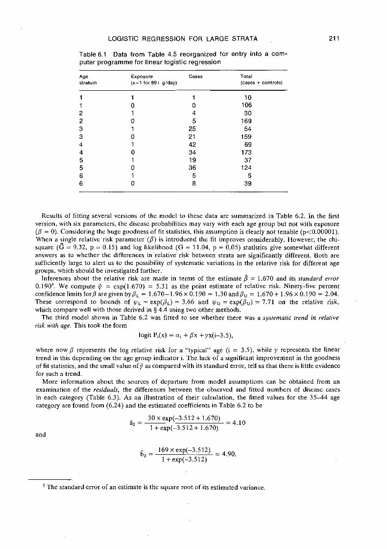
Example: To illustrate these calculations we reanalyse the grouped data from the Ille-et-Vilaine study of oesophageal cancer summarized in Table 4.1. Here the six strata are defined as ten-year age groups from 25-34 through 75+ years, while average alcohol consumption is treated as a binary risk factor with 0-79 g/day (up to one litre of wine) representing "unexposed" and anything over this amount "exposed". The data would be rearranged for computer entry as shown in Table 6.1, where 12 risk categories or groups are defined by the six strata and two levels of exposure. Within each of these the total N of cases + controls is regarded as the denominator of an observed disease proportion, while'the number of cases is the numerator. The numerical results should be compared closely with those already obtained in 8 4.4.
LOGISTIC REGRESSION FOR LARGE STRATA
Table 6.1 Data from Table 4.5 reorganized for entry into a com- puter programme for linear logistic regression
Age Exposure Cases Total stratum (x=l for 80+ glday) (cases + controls)
Results of fitting several versions of the model to these data are summarized in Table 6.2. In the first version, with six parameters, the disease probabilities may vary with each age group but not with exposure (/? = 0). Considering the huge goodness of fit statistics, this assumption is clearly not tenable (p<0.00001). When a single relative risk parameter (/3) is introduced the fit improves considerably. However, the chi- square (6 = 9.32, p = 0.15) and log likelihood (G = 11.04, p = 0.05) statistics give somewhat different answers as to whether the differences in relative risk between strata are significantly different. Both are sufficiently large to alert us to the possibility of systematic variations in the relative risk for different age groups, which should be investigated further.
Inferences about the relative risk are made in terms of the estimate f i = 1.670 and its standard error 0.190'. We compute $ = exp(1.670) = 5.31 as the point estimate of relative risk. Ninety-five percent confidence limits for/? are given by/?, = 1.670-1.96 x 0.190 = 1.30 andPU = 1.670 + 1.96 x 0.190 = 2.04. These correspond to bounds of y l , = exp(pL) = 3.66 and yiu = exp(/?,) = 7.71 on the relative risk, which compare well with those derived in § 4.4 using two other methods.
The third model shown in Table 6.2 was fitted to see whether there was a systematic trend in relative risk with age. This took the form
where now /? represents the log relative risk for a "typical" age (i = 3.5), while y represents the linear trend in this depending on the age group indicator i. The lack of a significant improvement in the goodness of fit statistics, and the small value of 7 as compared with its standard error, tell us that there is little evidence for such a trend.
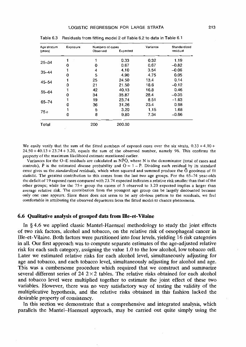
More information about the sources of departure from model assumptions can be obtained from an examination of the residuals, the differences between the observed and fitted numbers of disease cases in each category (Table 6.3). As an illustration of their calculation, the fitted values for the 35-44 age category are found from (6.24) and the estimated coefficients in Table 6.2 to be
and
' The standard error of an estimate is the square root of its estimated variance.
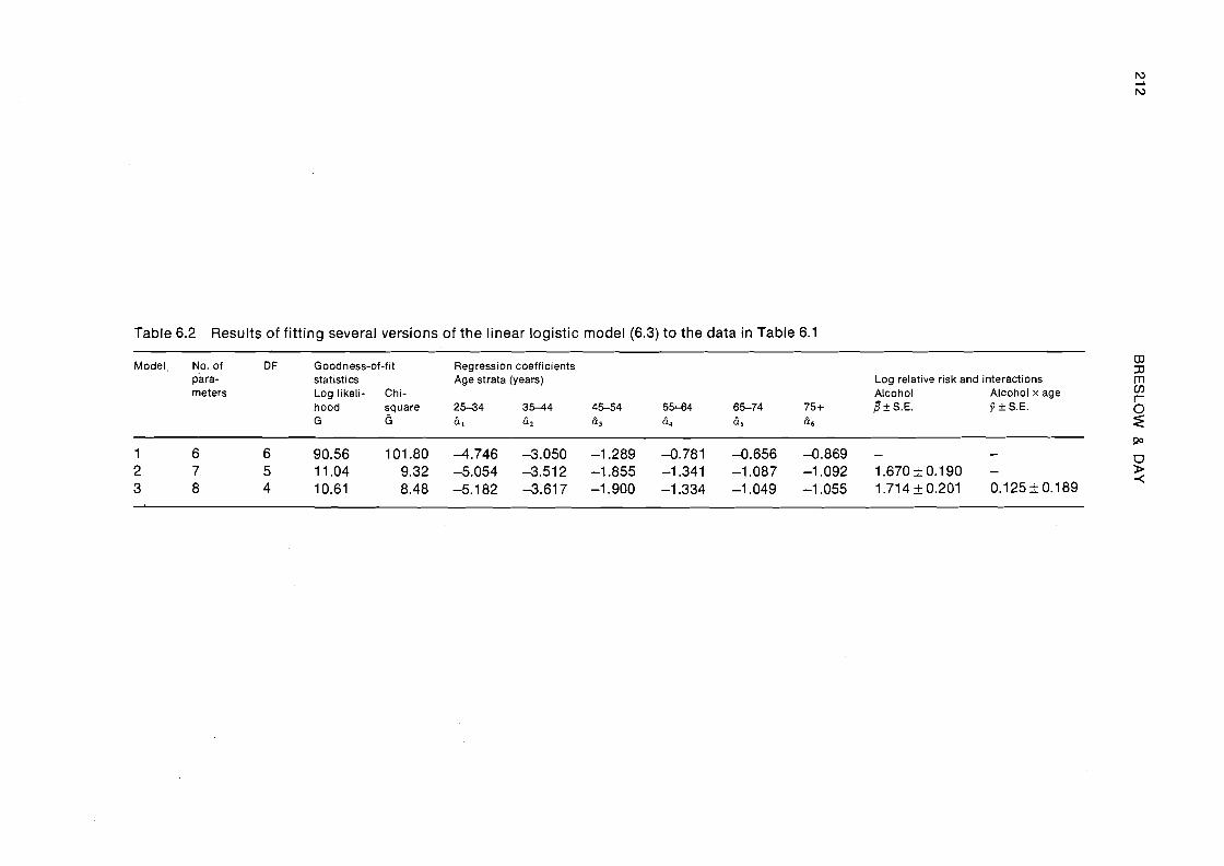
Table 6.2 Results of fitting several versions of the linear logistic model (6.3) to the data in Table 6.1
Model, No, of D F Goodness-of-fit Regression coefficients para- statistics Age strata (years) Log relative risk and interactions
% rn
meters Log likeli- Chi- Alcohol Alcohol x age V)
hood square 25-34 35-44 45-54 5544 65-74 75+ f l + S.E. 3 + S.E. G 6 61 6 2 f i3 h4 65 66
6 z
LOGISTIC REGRESSION FOR LARGE STRATA
Table 6.3 Residuals from fitting model 2 of Table 6.2 to data in Table 6.1
Age stratum Exposure Numbers of cases Variance Standardized (Years) Observed Expected residual
Total 200 200.00
We easily verify that the sum of the fitted numbers of exposed cases over the six strata, 0.33 +4.10+ 24.50+40.13 +23.74+ 3.20, equals the sum of the observed number, namely 96. This confirms the property of the maximum likelihood estimate mentioned earlier.
Variances for the 0-E residuals are calculated as NPQ, where N is the denominator (total of cases and controls), P is the estimated disease probability and Q = 1 - P. Dividing each residual by its standard error gives us the standardized residuals, which when squared and summed produce the 6 goodness of fit statistic. The greatest contribution to this comes from the last two age groups. For the 65-74 year-olds the deficit of 19 exposed cases compared with 23.74 expected indicates a relative risk smaller than that of the other groups; while for the 75+ group the excess of 5 observed to 3.20 expected implies a larger than average relative risk. The contribution from the youngest age group can be largely discounted because only one case appears. Since there does not seem to be any obvious pattern to the residuals, we feel comfortable in attributing the observed departures from the fitted model to chance phenomena.
6.6 Qualitative analysis of grouped data from Ille-et-Vilaine
In 5 4.6 we applied classic Mantel-Haenszel methodology to study the joint effects of two risk factors, alcohol and tobacco, on the relative risk of oesophageal cancer in Ille-et-Vilaine. Both factors were partitioned into four levels, yielding 16 risk categories in all. Our first approach was to compute separate estimates of the age-adjusted relative risk for each such category, assigning the value 1.0 to the low alcohol, low tobacco cell. Later we estimated relative risks for each alcohol level, simultaneously adjusting for age and tobacco, and each tobacco level, simultaneously adjusting for alcohol and age. This was a cumbersome procedure which required that we construct and summarize several different series of 24 2 x 2 tables. The relative risks obtained for each alcohol and tobacco level were multiplied together to estimate the joint effect of these two variables. However, there was no very satisfactory way of testing the validity of the multiplicative hypothesis, and the relative risks obtained in this fashion lacked the desirable property of consistency.
In this section we demonstrate that a comprehensive and integrated analysis, which parallels the Mantel-Haenszel approach, may be carried out quite simply using the
21 4 BRESLOW & DAY
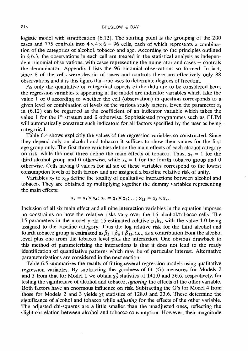
logistic model with stratification (6.12). The starting point is the grouping of the 200 cases and 775 controls into 4 x 4 x 6 = 96 cells, each of which represents a combina- tion of the categories of alcohol, tobacco and age. According to the principles outlined in 5 6.3, the observations in each cell are trea+.ed in the statistical analysis as indepen- dent binomial observations, with cases representing the numerator and cases + controls the denominator. Appendix I lists the 96 binomial observations so formed. In fact, since 8 of the cells were devoid of cases and controls there are effectively only 88 observations and it is this figure that one uses to determine degrees of freedom.
As only the qualitative or categorical aspects of the data are to be considered here, the regression variables x appearing in the model are indicator variables which take the value 1 or 0 according to whether the cell (observation) in question corresponds to a given level or combination of levels of the various study factors. Even the parameter ai in (6.12) can be regarded as the coefficient of an indicator variable which takes the value 1 for the ith stratum and 0 otherwise. Sophisticated programmes such as GLIM will automatically construct such indicators for all factors specified by the user as being categorical.
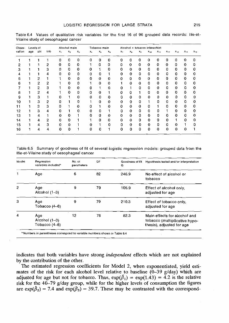
Table 6.4 shows explicitly the values of the regression variables so constructed. Since they depend only on alcohol and tobacco it suffices to show their values for the first age group only. The first three variables define the main effects of each alcohol category on risk, while the next three define the main effects of tobacco. Thus, x2 = 1 for the third alcohol group and 0 otherwise, while = 1 for the fourth tobacco group and 0 otherwise. Cells having 0 values for all six of these variables correspond to the lowest consumption levels of both factors and are assigned a baseline relative risk of unity.
Variables x7 to x15 define the totality of qualitative interactions between alcohol and tobacco. They are obtained by multiplying together the dummy variables representing the main effects:
Inclusion of all six main effect and all nine interaction variables in the equation imposes no constraints on how the relative risks vary over the l(j alcohol/tobacco cells. The 15 parameters in the model yield 15 estimated relative risks, with the value 1.0 being assigned to the baseline category. Thus the log relative risk for the third alcohol and fourth tobacco group is estimated as 8, +b6 +BIZ, i.e., as a contribution from the alcohol level plus one from the tobacco level plus the interaction. One obvious drawback to this method of parameterizing the interactions is that it does not lead to the ready identification of quantitative patterns which may be of particular interest. Alternative parameterizations are considered in the next section.
Table 6.5 summarizes the results of fitting several regression models using qualitative regression variables, By subtracting the goodness-of-fit (G) measures for Models 2 and 3 from that for Model 1 we obtain X: statistics of 141.0 and 36.6, respectively, for testing the significance of alcohol and tobacco, ignoring the effects of the other variable. Both factors have an enormous influence on risk. Subtracting the G's for Model 4 from those for Models 2 and 3 yields X: statistics of 128.0 and 23.6. These determine the significance of alcohol and tobacco while adjusting for the effects of the other variable. The adjusted chi-squares are a little smaller than the unadjusted ones, reflecting the slight correlation between alcohol and tobacco consumption. However, their magnitude
LOGISTIC REGRESSION FOR LARGE STRATA 215
Table 6.4 Values of qualitative risk variables for the first 16 of 96 grouped data records: Ille-et- Vilaine study of oesophageal cancer
Obser- Levels of Alcohol main Tobacco main Alcohol x tobacco interaction vation age alc tob x , x, x3 X4 X~ X6 x 7 XB x 9 XIO X~~ X~~ X13 X14 X~~
Table 6.5 Summary of goodness of fit of several logistic regression models: grouped data from the Ille-et-Vilaine study of oesophageal cancer
- - - - - - - - -
Model Regression No. of OF Goodness of fit Hypothesis tested and/or interpretation variables includeda parameters G
- - - - - -
6 82 246.9 No effect of alcohol or tobacco
2 Age 9 79 105.9 Effect of alcohol only, Alcohol ( 1 3 ) adjusted for age
3 Age 9 79 21 0.3 Effect of tobacco only, Tobacco (4-6) adjusted for age
- -- -- -
4 Age 12 76 82.3 Main effects for alcohol and Alcohol ( 1 3 ) tobacco (multiplicative hypo- Tobacco (4-6) thesis), adjusted for age
a Numbers in parentheses correspond to variable numbers shown in Table 6.4
indicates that both variables have strong independent effects which are not explained by the contribution of the other.
The estimated regression coefficients for Model 2, when exponentiated, yield esti- mates of the risk for each alcohol level relative to baseline (0-39 g/day) which are adjusted for age but not for tobacco. Thus, exp@,) = exp(1.43) = 4.2 is the relative risk for the 40-79 g/day group, while for the higher levels of consumption the figures are exp(),) = 7.4 and exp@,) = 39.7. These may be contrasted with the correspond-
BRESLOW & DAY
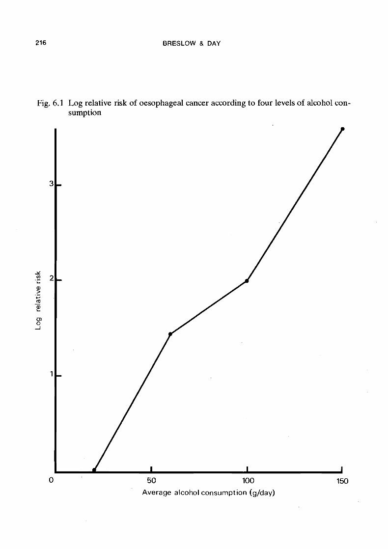
Fig. 6.1 Log relative risk of oesophageal cancer according to four levels of alcohol con- sumption
Average alcohol consumption (glday)
LOGISTIC REGRESSION FOR LARGE STRATA 21 7
ing figures of 4.3, 8.0 and 28.6 obtained by the Mantel-Haenszel (M-H) method (Table 4.4). There is reasonably good agreement except for the highest exposure category, where there were few cases and controls in some strata. For this category the conditional maximum likelihood estimate (5 4.4) was 34.9, midway between the M-H estimate and unconditional MLE. The latter estimate is probably a bit exaggerated here because of the thin data (5 7.1).
One disadvantage of the elementary methods was that the relative risks obtained upon varying the choice of baseline category were not consistent. For example, the direct M-H estimate of the risk for the fourth alcohol level relative to the second is 8.7 rather than 28.6/4.3 = 6.7. Use of the logistic modelling approach avoids such
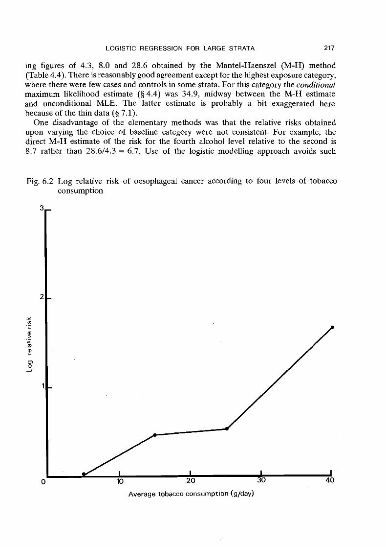
Fig. 6.2 Log relative risk of oesophageal cancer according to four levels of tobacco consumption
Average tobacco consumption (g/day)
21 8 BRESLOW & DAY
discrepancies. Estimates of the log relative risks between any two categories are always obtained as the differences in the regression coefficients for those categories (with the proviso that the coefficient for the baseline category is O), and such differences are not affected by the choice of the baseline category. Thus exp(), -8,) = 9.4 represents the risk of level four relative to level two regardless of how the indicator variables repre- senting the alcohol effects are coded.
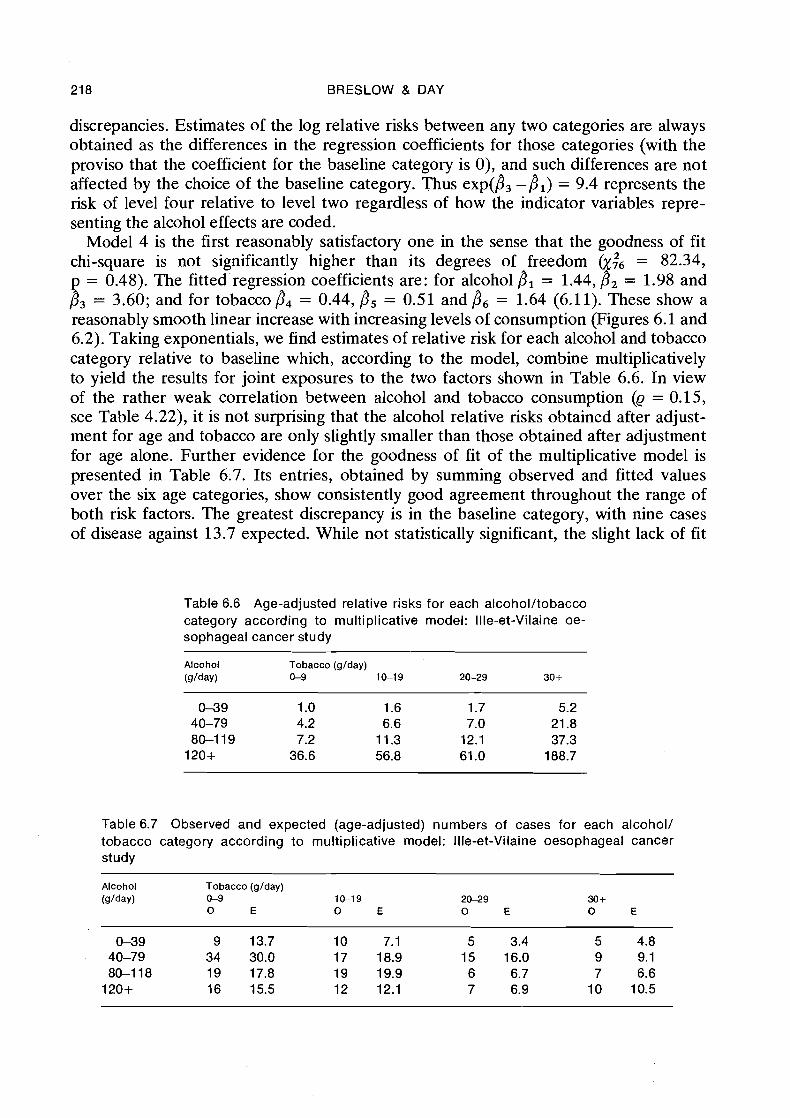
Model 4 is the first reasonably satisfactory one in the sense that the goodness of fit chi-square is not significantly higher than its degrees of freedom 01;6 = 82.34, p = 0.48). The fitted regression coefficients are: for alcohol 8, = 1.44, 8, = 1.98 and 8, = 3.60; and for tobacco fi4 = 0.44, B5 = 0.51 and 8, = 1.64 (6.11). These show a reasonably smooth linear increase with increasing levels of consumption (Figures 6.1 and 6.2). Taking exponentials, we find estimates of relative risk for each alcohol and tobacco category relative to baseline which, according to the model, combine multiplicatively to yield the results for joint exposures to the two factors shown in Table 6.6. In view of the rather weak correlation between alcohol and tobacco consumption (Q = 0.15, see Table 4.22), it is not surprising that the alcohol relative risks obtained after adjust- ment for age and tobacco are only slightly smaller than those obtained after adjustment for age alone. Further evidence for the goodness of fit of the multiplicative model is presented in Table 6.7. Its entries, obtained by summing observed and fitted values over the six age categories, show consistently good agreement throughout the range of both risk factors. The greatest discrepancy is in the baseline category, with nine cases of disease against 13.7 expected. While not statistically significant, the slight lack of fit
Table 6.6 Age-adjusted relative risks for each alcohol/tobacco category according to multiplicative model: Ille-et-Vilaine oe- sophageal cancer study
Alcohol Tobacco (glday) (g lda~ ) 0-9 1&19 20-29 30+
Table 6.7 Observed and expected (age-adjusted) numbers of cases for each alcohol/ tobacco category according to multiplicative model: Ille-et-Vilaine oesophageal cancer study
Alcohol Tobacco (glday) (glday) &9 1&19 2&29 30+
0 E 0 E 0 E 0 E
LOGISTIC REGRESSION FOR LARGE STRATA 21 9
for this category indicates that the relative risk for the other levels of exposure might possibly be even greater than that suggested by the model.
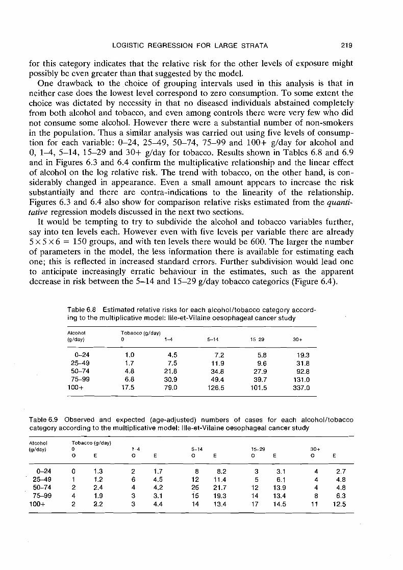
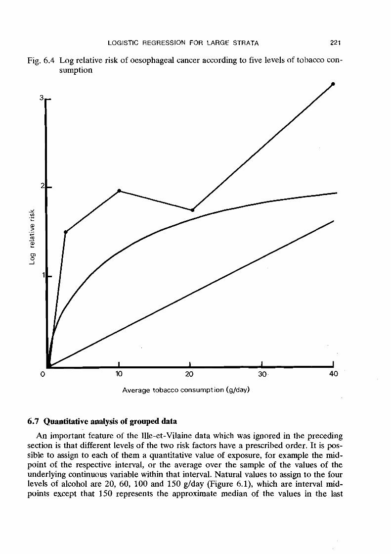
One drawback to the choice of grouping intervals used in this analysis is that in neither case does the lowest level correspond to zero consumption. To some extent the choice was dictated by necessity in that no diseased individuals abstained completely from both alcohol and tobacco, and even among controls there were very few who did not consume some alcohol. However there were a substantial number of non-smokers in the population. Thus a similar analysis was carried out using five levels of consump- tion for each variable: 0-24, 2 5 4 9 , 50-74, 75-99 and 100+ g/day for alcohol and 0, 1-4, 5-14, 15-29 and 30+ g/day for tobacco. Results shown in Tables 6.8 and 6.9 and in Figures 6.3 and 6.4 confirm the multiplicative relationship and the linear effect of alcohol on the log relative risk. The trend with tobacco, on the other hand, is con- siderably changed in appearance. Even a small amount appears to increase the risk substantially and there are contra-indications to the linearity of the relationship. Figures 6.3 and 6.4 also show for comparison relative risks estimated from the quanti- tative regression models discussed in the next two sections.
It would be tempting to try to subdivide the alcohol and tobacco variables further, say into ten levels each. However even with five levels per variable there are already 5 x 5 x 6 = 150 groups, and with ten levels there would be 600. The larger the number of parameters in the model, the less information there is available for estimating each one; this is reflected in increased standard errors. Further subdivision would lead one to anticipate increasingly erratic behaviour in the estimates, such as the apparent decrease in risk between the 5-14 and 15-29 g/day tobacco categories (Figure 6.4).
Table 6.8 Estimated relative risks for each alcohol/tobacco category accord- ing to the multiplicative model: Ille-et-Vilaine oesophageal cancer study
Alcohol Tobacco (glday) @/day) 0 1 4 5-1 4 15-29 30 +
Table6.9 Observed and expected (age-adjusted) numbers of cases for each alcohol/tobacco category according to the multiplicative model: Ille-et-Vilaine oesophageal cancer study
Alcohol Tobacco (glday) (glday) 0 1 4 5-14 1 5 2 9 30+
0 E 0 E 0 E 0 E 0 E
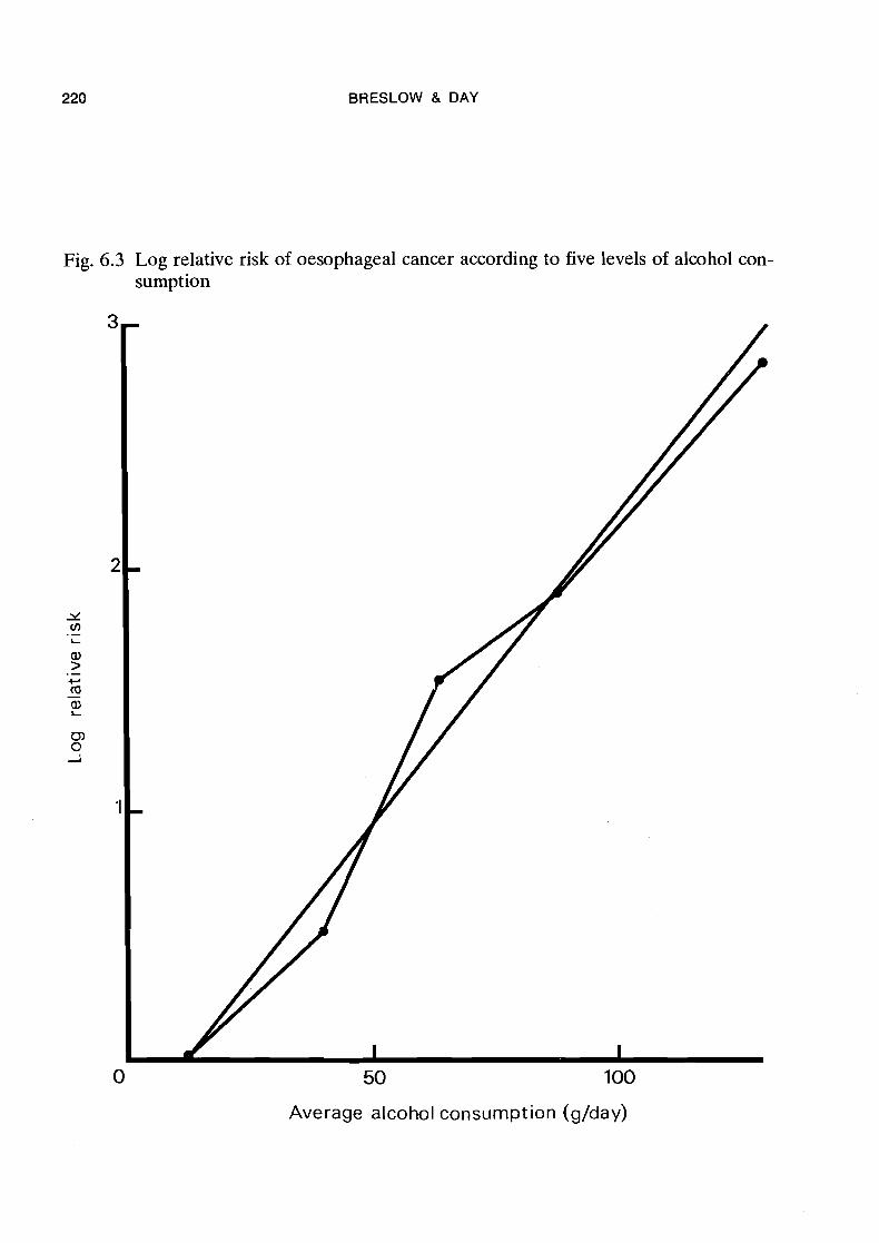
Fig.
BRESLOW & DAY
6.3 Log relative risk of oesophageal cancer according to five levels of alcohol con- sumption
50 100
Average alcohol consumption (glday)
LOGISTIC REGRESSION FOR LARGE STRATA 221
Fig. 6.4 Log relative risk of oesophageal cancer according to five levels of tobacco con- sumption
10 20 30 -
Average tobacco consumption (g/day)
6.7 Quantitative analysis of grouped data
An important feature of the Ille-et-Vilaine data which was ignored in the preceding section is that different levels of the two risk factors have a prescribed order. It is pos- sible to assign to each of them a quantitative value of exposure, for example the mid- point of the respective interval, or the average over the sample of the values of the underlying continuous variable within that interval. Natural values to assign to the four levels of alcohol are 20, 60, 100 and 150 g/day (Figure 6.1), which are interval mid- points except that 150 represents the approximate median of the values in the last
222 BRESLOW & DAY
open-ended interval above 120 glday. Similarly, for tobacco, natural values are 5, 15, 25 and 40 glday (Figure 6.2). Even the stratification variable is quantitative, with equally-spaced intervals centred about 30, 40, 50, 60, 70 and 80 years of age.
Quantitative aspects of the data may be accounted for in the analysis by using con- tinuous regression variables in place of the categorical ones. There are several advantages in this approach. First, the data can often be adequately summarized by a smaller number of parameters, which facilitates interpretation. Tests for the significance of individual regression coefficients are single degree of freedom tests for trend which, as we have repeatedly emphasized, are generally more powerful than tests directed against global alternatives to the null hypothesis. This feature is especially important in exploring possible interactions, since chi-square statistics based on qualitative inter- action variables tend to have rather large numbers of degrees of freedom. Quantitative interaction variables, obtained as the product of the quantitative variables representing the main effects of the corresponding factors, enable us to identify particular patterns of departure from the basic linear model.
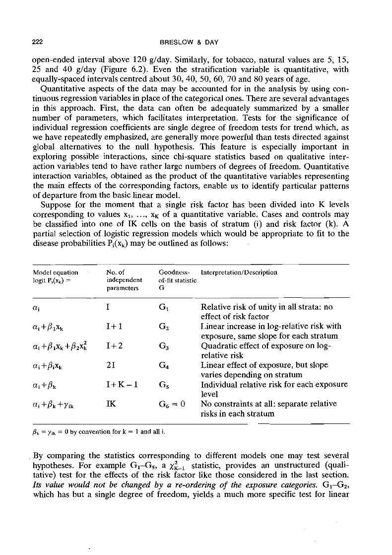
Suppose for the moment that a single risk factor has been divided into K levels corresponding to values XI, .. ., x~ of a quantitative variable. Cases and controls may be classified into one of IK cells on the basis of stratum (i) and risk factor (k). A partial selection of logistic regression models which would be appropriate to fit to the disease probabilities Pi(xk) may be outlined as follows:
Model equation No. of Goodness- Interpretation/Description logit Pi(xk) = independent of-fit statistic
parameters G
i I GI Relative risk of unity in all strata: no effect of risk factor
ai+plxk I + 1 G2 Linear increase in log-relative risk with exposure, same slope for each stratum
ai +@ixk +@2~: 1 + 2 G3 Quadratic effect of exposure on log- relative risk
ai +pix, 21 G4 Linear effect of exposure, but slope varies depending on stratum
ai+pk I + K - 1 G5 Individual relative risk for each exposure level
ai +pk+~ik IK G6 = o NO constraints at all: separate relative risks in each stratum
pk = yik = 0 by convention for k = 1 and all i .
By comparing the statistics corresponding to different models one may test several 2 hypotheses. For example GI-G,, a x,, statistic, provides an unstructured (quali-
tative) test for the effects of the risk factor like those considered in the last section. Its value would not be changed by a re-ordering of the exposure categories. G I G 2 , which has but a single degree of freedom, yields a much more specific test for linear
LOGISTIC REGRESSION FOR LARGE STRATA 223
trend in log relative risk with increasing exposure. A global test of departures from the linear' model is provided by Gz-G5, on K-2 degrees of freedom, while Gz-G3 is a X: statistic specifically designed to test for curvature in the regression line. Finally, Gz-Gq is a xi-' statistic testing the parallelism of the regression lines in the I strata. Lack of parallelism means that the relative risks for different exposure levels vary from one stratum to another, i.e., that there are interactions between stratification variables and risk factors. Notice that the goodness-of-fit statistic for model 6 is 0. Since the number of independent parameters equals the number of observations, there is perfect agreement between model and data in this case.
A similar but somewhat more elaborate set of models was fitted to the 96 grouped data records from Ille-et-Vilaine, treating fhe two risk factors alternately as qualitative and quantitative variables at four levels'each. The values assigned to each level are as indicated. above, namely 20, 60, 100 and 150 g/day for alcohol and 5, 15, 25 and 40 g/day for tobacco. In fact these x values were not used in the regression analyses in their original form, since this would have led to computational problems, especially with the square terms. Instead, alcohol consumption was expressed in units of 100 g/day, with values 0.2, 0.6, 1.0 and 1.5, while tobacco was expressed in units of 10 g/day. It is sometimes helpful to go even further and to standardize all regression variables, i.e., scale and centre them so that they have approximate mean values of zero and variances of unity, before proceeding with the numerical analyses.
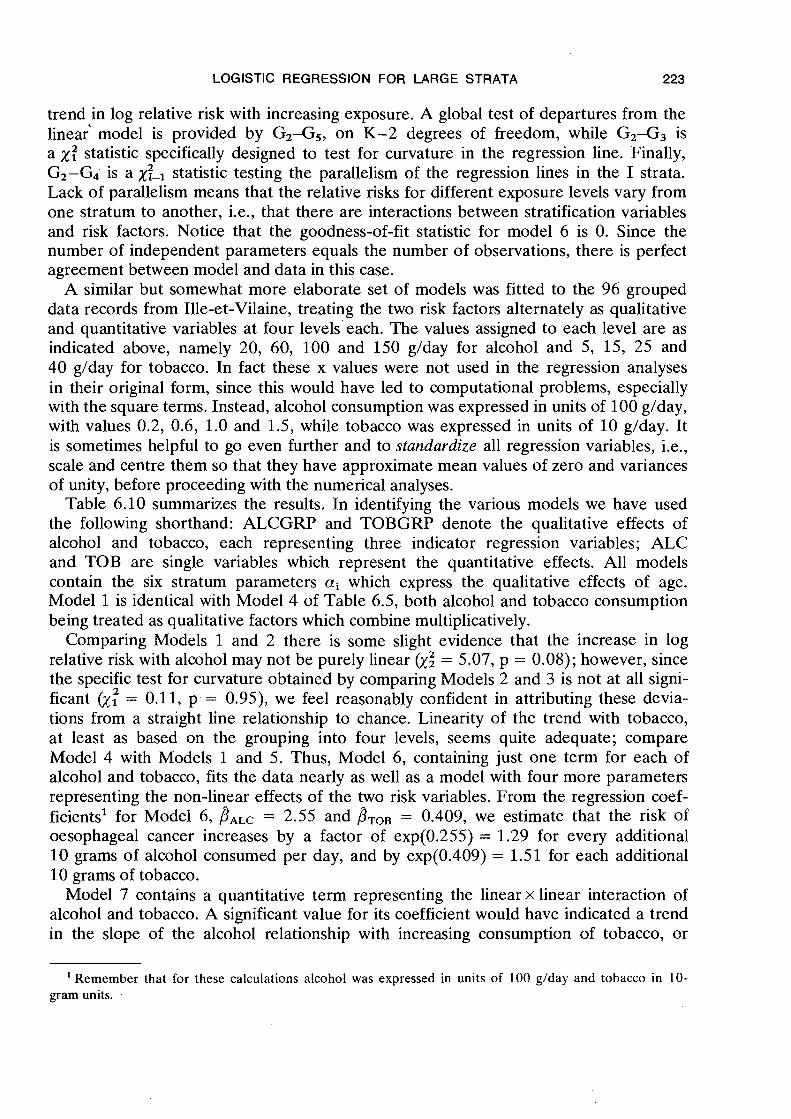
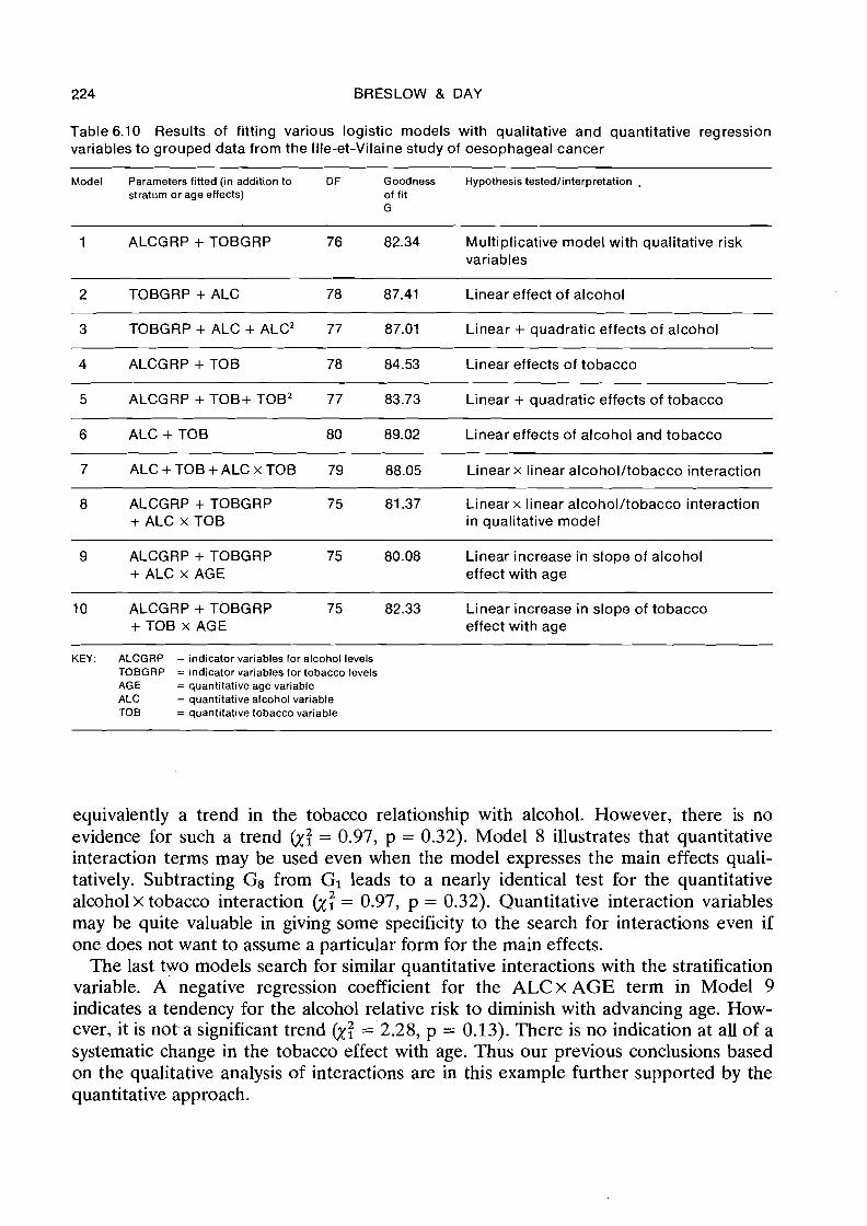
Table 6.10 summarizes the results. In identifying the various models we have used the following shorthand: ALCGRP and TOBGRP denote the qualitative effects of alcohol and tobacco, each representing three indicator regression variables; ALC and TOB are single variables which represent the quantitative effects. All models contain the six stratum parameters ai which express the qualitative effects of age. Model 1 is identical with Model 4 of Table 6.5, both alcohol and tobacco consumption being treated as qualitative factors which combine multiplicatively.
Comparing Models 1 and 2 there is some slight evidence that the increase in log relative risk with alcohol may not be purely linear (y; = 5.07, p = 0.08); however, since the specific test for curvature obtained by comparing Models 2 and 3 is not at all signi- ficant (y: = 0.11, p = 0.95), we feel reasonably confident in attributing these devia- tions from a straight line relationship to chance. Linearity of the trend with tobacco, at least as based on the grouping into four levels, seems quite adequate; compare Model 4 with Models 1 and 5. Thus, Model 6, containing just one term for each of alcohol and tobacco, fits the data nearly as well as a model with four more parameters representing the non-linear effects of the two risk variables. From the regression coef- ficients' for Model 6, bALc = 2.55 and b,, = 0.409, we estimate that the risk of oesophageal cancer increases by a factor of exp(0.255) = 1.29 for every additional 10 grams of alcohol consumed per day, and by exp(0.409) = 1.51 for each additional 10 grams of tobacco.
Model 7 contains a quantitative term representing the linear x linear interaction of alcohol and tobacco. A significant value for its coefficient would have indicated a trend in the slope of the alcohol relationship with increasing consumption of tobacco, or
' Remember that for these calculations alcohol was expressed in units of 100 g/day and tobacco in 10- gram units.
224 BRESLOW & DAY
Table 6.10 Results of fitting various logistic models with qualitative and quantitative regression variables to grouped data from the Ille-et-Vilaine study of oesophageal cancer
Model Parameters fitted (in addition to DF Goodness Hypothesis testedlinterpretation , stratum or age effects) of fit
G - - - - - - - - -
1 ALCGRP + TOBGRP 76 82.34 Multiplicative model with qualitative risk variables
2 TOBGRP + ALC 78 87.41 Linear effect of alcohol - - - -
3 TOBGRP + ALC + ALCZ 77 87.01 Linear + quadratic effects of alcohol
4 ALCGRP + TOB 78 84.53 Linear effects of tobacco
5 ALCGRP + TOB+ TOB2 77 83.73 Linear + quadratic effects of tobacco
6 ALC + TO6 80 89.02 Linear effects of alcohol and tobacco
7 ALC + TOB + ALC x TOB 79 88.05 Linear x linear alcohol/tobacco interaction
8 ALCGRP + TOBGRP 75 81.37 Linear x linear alcohol/tobacco interaction + ALC x TOB in qualitative model
9 ALCGRP + TOBGRP 75 80.08 Linear increase i'n slope of alcohol + ALC x AGE effect with age
10 ALCGRP + TOBGRP 75 82.33 Linear increase in slope of tobacco + TOB x AGE effect with age
KEY: ALCGRP = indicator variables for alcohol levels TOBGRP = indicator variables for tobacco levels AGE = quantitative age variable ALC = quantitative alcohol variable TOB = quantitative tobacco variable
equivalently a trend in the tobacco relationship with alcohol. However, there is no evidence for such a trend &: = 0.97, p = 0.32). Model 8 illustrates that quantitative interaction terms may be used even when the model expresses the main effects quali- tatively. Subtracting G8 from GI leads to a nearly identical test for the quantitative alcoholx tobacco interaction &: = 0.97, p = 0.32). Quantitative interaction variables may be quite valuable in giving some specificity to the search for interactions even if one does not want to assume a particular form for the main effects.
The last two models search for similar quantitative interactions with the stratification variable. A negative regression coefficient for the ALCx AGE term in Model 9 indicates a tendency for the alcohol relative risk to diminish with advancing age. How- ever, it is not. a significant trend &; = 2.28, p = 0.13). There is no indication at all of a systematic change in the tobacco effect with age. Thus our previous conclusions based on the qualitative analysis of interactions are in this example further supported by the quantitative approach.
LOGISTIC REGRESSION FOR LARGE STRATA 225
6.8 Regression adjustment for confounders
Stratification, whether in the context of M-H methodology or logistic regression, has traditionally been used to control the confounding effects of nuisance factors. Typically, we define a separate stratum for each combination of levels of the nuisance factors, assigning to each one a parameter in the model. If there are several such factors, or if they occur at very many levels, the total number of strata can become quite large. For example, with three stratifying factors at 3, 4 and 5 levels, respectively, the total number of a parameters in (6.2) is 3 x 4 x 5 = 60. Since the available data usually place severe limitations on the number of strata which may be incorporated in the analysis, alter- native methods for the control of confounding must be considered.
From the discussion in 5 6.1 it is clear that the practice of stratification is tantamount to saturating the effects of the nuisance factors with parameters. Not only the main effects, but also all the first and higher order interaction terms are represented. This practice is unnecessary, however, unless we have good reason to believe that such higher order interactions are present. An obvious alternative to stratification for the control of confounding variables is to incorporate their effects directly into the model. This allows us much more flexibility in deciding which of the higher order interaction terms to retain and which to discard. The approach may be especially efficacious with continuous nuisance factors whose effects can be adequately summarized in a few quantitative regression variables.
This does not mean, however, that risk and nuisance variables are treated sym- metrically in the analysis. For risk factors our goal is to identify the most important ones and quantify their influence in a precise and meaningful way. This implies that we economize on the number of parameters used to represent them and that we retain in the multivariate risk equation only those which have reasonably significant effects.
For nuisance factors, on the other hand, the effects on disease have presumably already been conceded, or in any event are not the specific concern of the study. They are included only to ensure that the estimates of relative risk are free from possible confounding effects, and no specific meaning is to be attached to their coefficients. Hence, known confounding variables should be included in the equation regardless of statistical significance if such inclusion changes the estimated coefficients of the risk variables by any appreciable degree (5 3.4).
We illustrate the regression adjustment for confounding effects with the grouped data from llle-et-Vilaine, specifically the age adjustment of estimates in the qualitative multiplicative model (Model 4, Table 6.5). Table 6.1 1 compares the previous estimates, obtained using stratification in six age groups, to estimates for which quantitative adjustments were made by introducing polynomial expressions in age group into the equation. Let i denote the age stratum, j the alcohol group, and k the tobacco group. The left-hand column presents the unadjusted estimates, based on an equation of the form
where age does not appear at all. The next column shows the changes in .the alcohol and tobacco coefficients upon introduction of a single linear term in age
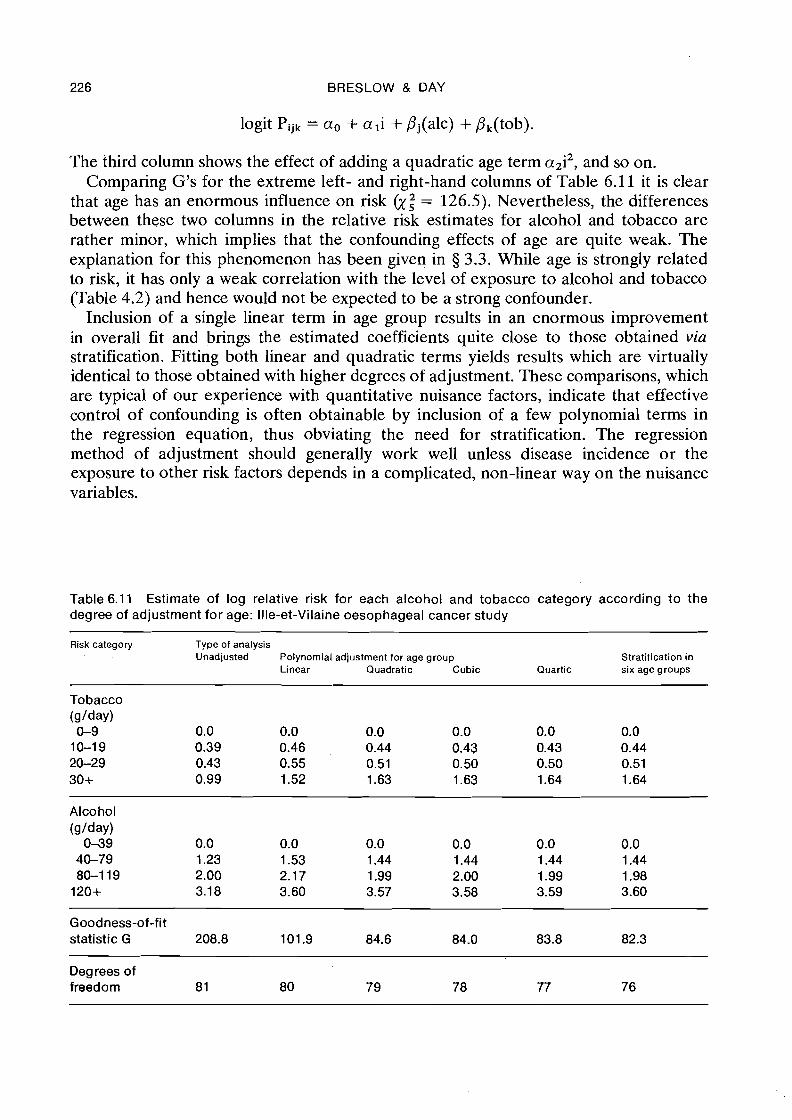
226 BRESLOW & DAY
logit Pijk = a. + a l i + pj(alc) + pk(tob).
The third column shows the effect of adding a quadratic age term a2i2, and so on. Comparing G's for the extreme left- and right-hand columns of Table 6.1 1 it is clear
that age has an enormous influence on risk (y,2 = 126.5). Nevertheless, the differences between these two columns in the relative risk estimates for alcohol and tobacco are rather minor, which implies that the confounding effects of age are quite weak. The explanation for this phenomenon has been given in 5 3.3. While age is strongly related to risk, it has only a weak correlation with the level of exposure to alcohol and tobacco (Table 4.2) and hence would not be expected to be a strong confounder.
Inclusion of a single linear term in age group results in an enormous improvement in overall fit and brings the estimated coefficients quite close to those obtained via stratification. Fitting both linear and quadratic terms yields results which are virtually identical to those obtained with higher degrees of adjustment. These comparisons, which are typical of our experience with quantitative nuisance factors, indicate that effective control of confounding is often obtainable by inclusion of a few polynomial terms in the regression equation, thus obviating the need for stratification. The regression method of adjustment should generally work well unless disease incidence o r the exposure to other risk factors depends in a complicated, non-linear way on the nuisance variables.
Table 6.11 Estimate of log relative risk for each alcohol and tobacco category according to the degree of adjustment for age: Ille-et-Vilaine oesophageal cancer study
Risk category Type of analysis Unadjusted Polynomial adjustment for age group Stratification in
Linear Quadratic Cubic Quartic six age groups
Tobacco (glday) 0-9 0.0 0.0 0.0 0.0 0.0 0.0 10-19 0.39 0.46 0.44 0.43 0.43 0.44 20-29 0.43 0.55 0.51 0.50 0.50 0.51 30+ 0.99 1.52 1.63 1.63 1.64 1.64
Alcohol (glday) 0-39 0.0 0.0 0.0 0.0 0.0 0.0 40-79 1.23 1.53 1.44 1.44 1.44 1.44 80-1 19 2.00 2.17 1.99 2.00 1.99 1.98 120+ 3.1 8 3.60 3.57 3.58 3.59 3.60
Goodness-of-fit statistic G 208.8 101.9 84.6 84.0 83.8 82.3
Degrees of freedom 8 1 80 79 78 77 76
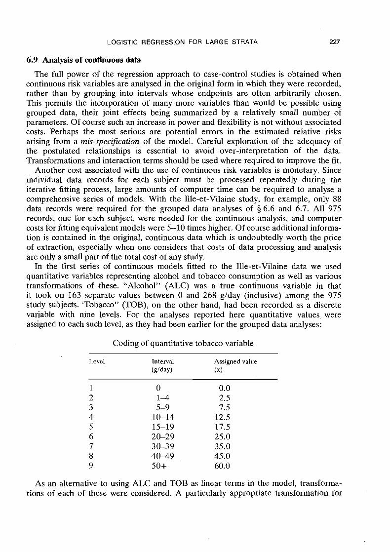
LOGISTIC REGRESSION FOR LARGE STRATA 227
6.9 Analysis of continuous data
The full power of the regression approach to case-control studies is obtained when continuous risk variables are analysed in the original form in which they were recorded, rather than by grouping into intervals whose endpoints are ofien arbitrarily chosen. This permits the incorporation of many more variables than would be possible using grouped data, their joint effects being summarized by a relatively small number of parameters. Of course such an increase in power and flexibility is not without associated costs. Perhaps the most serious are potential errors in the estimated relative risks arising from a rnis-specification of the model. Careful exploration of the adequacy of the postulated relationships is essential to avoid over-interpretation of the data. Transformations and interaction terms should be used where required to improve the fit.
Another cost associated with the use of continuous risk variables is monetary. Since individual data records for each subject must be processed repeatedly during the iterative fitting process, large amounts of computer time can be required to analyse a comprehensive series of models. With the llle-et-Vilaine study, for example, only 88 data records were required for the grouped data analyses of 5 6.6 and 6.7. All 975 records, one for each subject, were needed for the continuous analysis, and computer costs for fitting equivalent models were 5-10 times higher. Of course additional informa- tion is contained in the original, continuous data which is undoubtedly worth the price of extraction, especially when one considers that costs of data processing and analysis are only a small part of the total cost of any study.
In the first series of continuous models fitted to the llle-et-Vilaine data we used quantitative variables representing alcohol and tobacco consumption as well as various transformations of these. "Alcohol" (ALC) was a true continuous variable in that it took on 163 separate values between 0 and 268 g/day (inclusive) among the 975 study subjects. 'Tobacco" (TOB), on the other hand, had been recorded as a discrete variable with nine levels. For the analyses reported here quantitative values were assigned to each such level, as they had been earlier for the grouped data analyses:
Coding of quantitative tobacco variable
Level Interval Assigned value W a y ) (x)
As an alternative to using ALC and TOB as linear terms in the model, transforma- tions of each of these were considered. A particularly appropriate transformation for
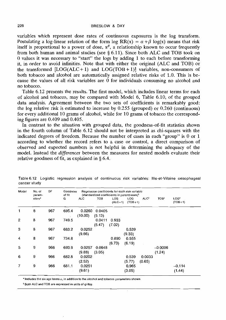
228 BRESLOW & DAY
variables which represent dose rates of continuous exposures is the log transform. Postulating a log-linear relation of the form log RR(x) = a +P log(x) means that risk itself is proportional to a power of dose, xp, a relationship known to occur frequently from both human and animal studies (see 5 6.11). Since both ALC and TOB took on 0 values it was necessary to "start" the logs by adding 1 to each before transforming it, in order to avoid infinities. Note that with either the original (ALC and TOB) or the transformed [LOG(ALC+ 1) and LOG(TOB+ I)] variables, non-consumers of both tobacco and alcohol are automatically assigned relative risks of 1.0. This is be- cause the values of all risk variables are 0 for individuals consuming no alcohol and no tobacco.
Table 6.12 presents the results. The first model, which includes linear terms for each of alcohol and tobacco, may be compared with Model 6, Table 6.10, of the grouped data analysis. Agreement between the two sets of coefficients is remarkably good: the log relative risk is estimated to increase by 0.255 (grouped) or 0.260 (continuous) for every additional 10 grams of alcohol, while for 10 grams of tobacco the correspond- ing .figures are 0.409 and 0.405.
In contrast to the situation with grouped data, the goodness-of-fit statistics shown in the fourth column of Table 6.12 should not be interpreted as chi-squares with the indicated degrees of freedom. Because the number of cases in each "group" is 0 or 1 according to whether the record refers to a case or control, a direct comparison of observed and expected numbers is not helpful in determining the adequacy of the model. Instead the differences between the measures for nested models evaluate their relative goodness of fit, as explained in 5 6.4.
Table 6.12 Logistic regression analysis of continuous risk variables: Ille-et-Vilaine oesophageal cancer study
Model No. of DF Goodness Regression coefficients for each risk variable param- of fit (standardized coefficients in par en these^)^ etersa G ALC TOB LOG LOG ALC2 TOB' LOG2
(ALCi1) (TOBi1) (TOBi1)
"Includes the six age terms ai in addition to the alcohol and tobacco parameters shown
Both ALC and TOB are expressed in units of g/day.
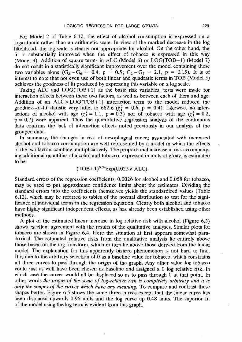
LOGISTIC REGRESSION FOR LARGE STRATA 229
For Model 2 of Table 6.12, the effect of alcohol consumption is expressed on a logarithmic rather than an arithmetic scale. In view of the marked decrease in the log likelihood, the log scale is clearly not appropriate for alcohol. On the other hand, the fit is substantially improved when the effect of tobacco is expressed in this way (Model 3). Addition of square terms in ALC (Model 6 ) o r LOG(TOB+l) (Model 7) do not result in a statistically significant improvement over the model containing these two variables alone (G3 - G6 = 0.4, p = 0.5; G2 -G7 = 2.1, p = 0.15). It is of interest to note that not even use of both linear and quadratic terms in TOB (Model 5) achieves the goodness of fit produced by expressing this variable on a log scale.
Taking ALC and LOG(TOB+l) as the basic risk variables, tests were made for interaction effects between these two factors, as well as between each of them and age. Addition of an ALCxLOG(TOB+I) interaction term to the model reduced the goodness-of-fit statistic very little, to 682.6 &: = 0.6, p = 0.4). Likewise, no inter- actions of alcohol with age &: = 1.1, p = 0.3) nor of tobacco with age &: = 0.2, p = 0.7) were apparent. Thus the quantitative regression analysis of the continuous data confirms the lack of interaction effects noted previously in our analysis of the grouped data.
In summary, the changes in risk of oesophageal cancer associated with increased alcohol and tobacco consumption are well represented by a model in which the effects of the two factors combine multiplicatively. The proportional increase in risk accompany- ing additional quantities of alcohol and tobacco, expressed in units of g/day, is estimated to be
(TOB+ 1)0-54exp(0.025 x ALC).
Standard errors of the regression coefficients, 0.0026 for alcohol and 0.058 for tobacco, may be used to put approximate confidence limits about the estimates. Dividing the standard errors into the coefficients themselves yields the standardized values (Table 6.12), which may be referred to tables of the normal distribution to test for the signi- ficance of individual terms in the regression equation. Clearly both alcohol and tobacco have highly significant independent effects, as has already been established using other methods.
A plot of the estimated linear increase in log relative risk with alcohol (Figure 6.3) shows excellent agreement with the results of the qualitative analyses. Similar plots for tobacco are shown in Figure 6.4. Here the situation at first appears somewhat para- doxical. The estimated relative risks from the qualitative analysis lie entirely above those based on the log transform, which in turn lie above those derived from the linear model. The explanation for this apparently bizarre phenomenon is not hard to find. It is due to the arbitrary selection of 0 as a baseline value for tobacco, which constrains all three curves to pass through the origin of the graph. Any other value for tobacco could just as well have been chosen as baseline and assigned a 0 log relative risk, in which case the curves would all be displaced so as to pass through 0 at that point. In other words the origin of the scale of log-relative risk is completely arbitrary and it is only the shapes of the curves which have any meaning. To compare and contrast these shapes better, Figure 6.5 shows the same three curves except that the linear curve has been displaced upwards 0.96 units and the log curve up 0.48 units. The superior fit of the model using the log term is evident from this graph.
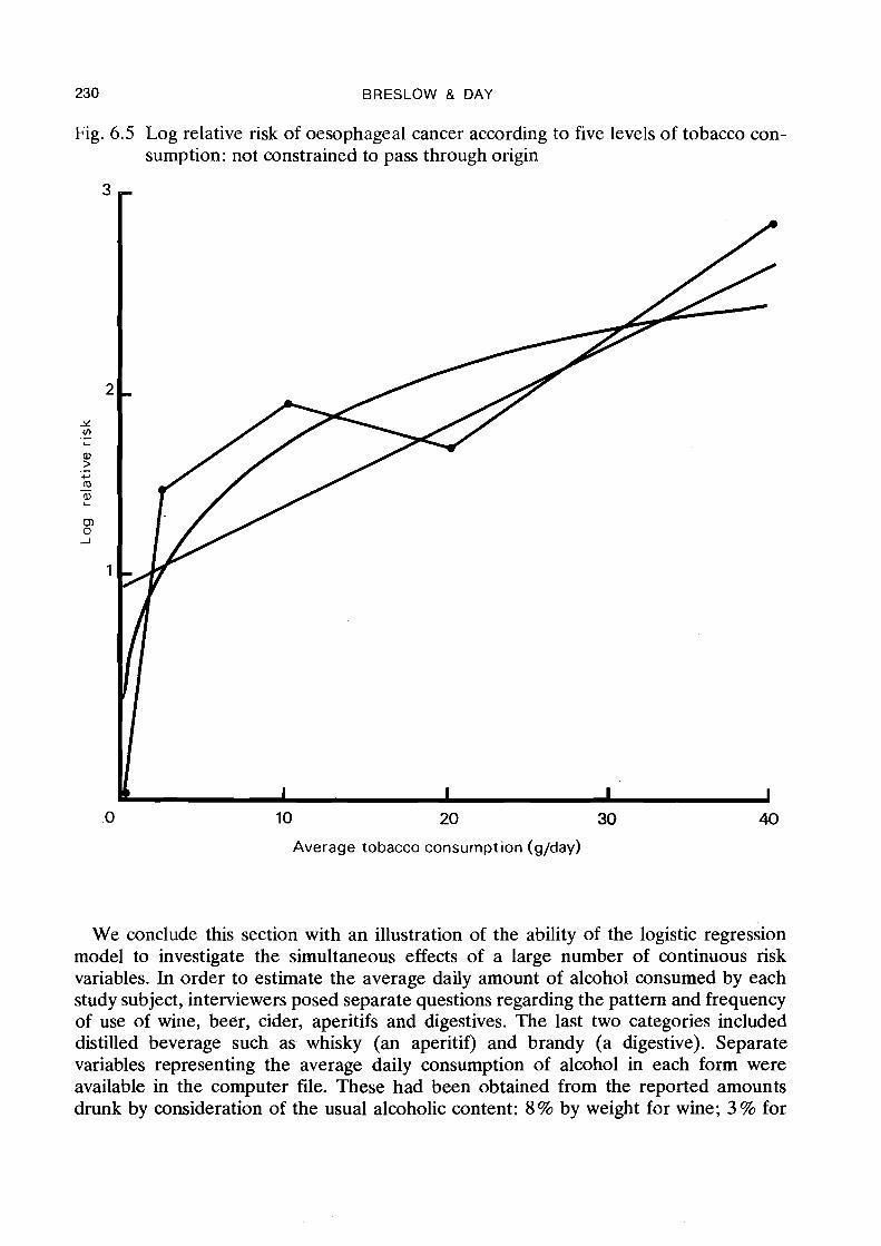
230 BRESLOW & DAY
Fig. 6.5 Log relative risk of oesophageal cancer according to five levels of tobacco con- sumption: not constrained to pass through origin
10 20 30
Average tobacco consumption (g/day)
We conclude this section with an illustration of the ability of the logistic regression model to investigate the simultaneous effects of a large number of continuous risk variables. In order to estimate the average daily amount of alcohol consumed by each study subject, interviewers posed separate questions regarding the pattern and frequency of use of wine, beer, cider, aperitifs and digestives. The last two categories included distilled beverage such a s whisky (an aperitif) and brandy (a digestive). Separate variables representing the average daily consumption of alcohol in each form were available in the computer file. These had been obtained from the reported amounts drunk by consideration of the usual alcoholic content: 8 % by weight for wine; 3 % for
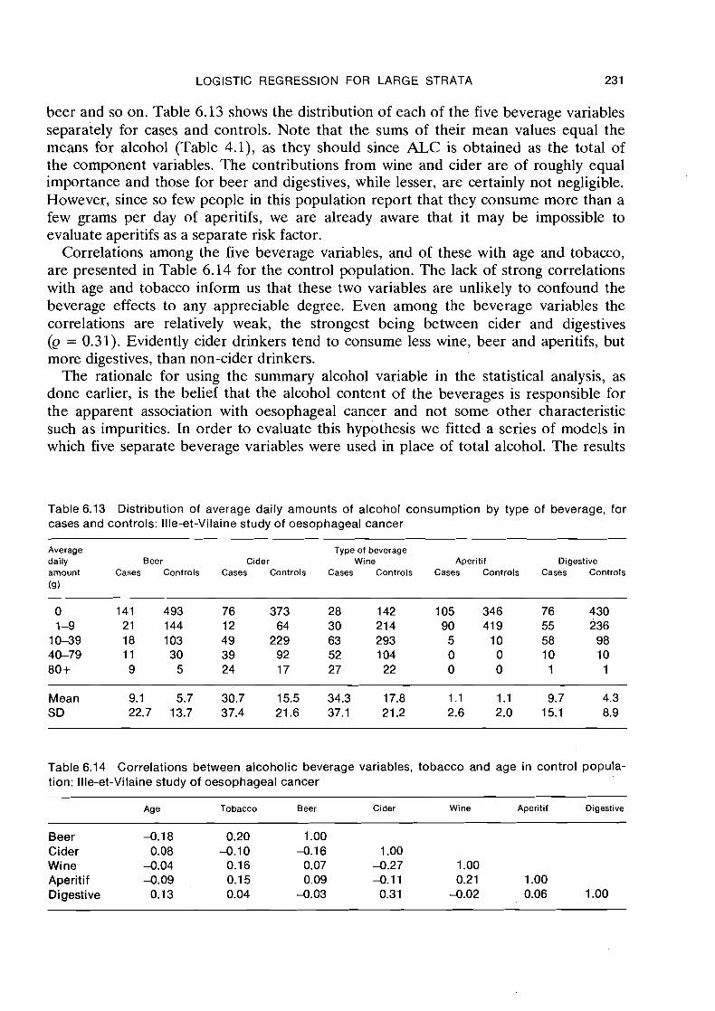
LOGISTIC REGRESSION FOR LARGE STRATA 23 1
beer and so on. Table 6.13 shows the distribution of each of the five beverage variables separately for cases and controls. Note that the sums of their mean values equal the means for alcohol (Table 4.1), as they should since ALC is obtained as the total of the component variables. The contributions from wine and cider are of roughly equal importance and those for beer and digestives, while lesser, are certainly not negligible. However, since so few people in this population report that they consume more than a few grams per day of aperitifs, we are already aware that it may be impossible to evaluate aperitifs as a separate risk factor.
Correlations among the five beverage variables, and of these with age and tobacco, are presented in Table 6.14 for the control population. The lack of strong correlations with age and tobacco inform us that these two variables are unlikely to confound the beverage effects to any appreciable degree. Even among the beverage variables the correlations are relatively weak, the strongest being between cider and digestives (Q = 0.31). Evidently cider drinkers tend to consume less wine, beer and aperitifs, but more digestives, than non-cider drinkers.
The rationale for using the summary alcohol variable in the statistical analysis, as done earlier, is the belief that the alcohol content of the beverages is responsible for the apparent association with oesophageal cancer and not some other characteristic such as impurities. In order to evaluate this hypothesis we fitted a series of models in which five separate beverage variables were used in place of total alcohol. The results
Table 6.13 Distribution of average daily amounts of alcohol consumption by type of beverage, for cases and controls: Ille-et-Vilaine study of oesophageal cancer
Average Type of beverage daily Beer Cider Wine Aperitif Digestive amount Cases Controls Cases Controls Cases Controls Cases Controls Cases Controls
(9)
Mean 9.1 5.7 30.7 15.5 34.3 17.8 1.1 1.1 9.7 4.3 SD 22.7 13.7 37.4 21.6 37.1 21.2 2.6 2.0 15.1 8.9
Table 6.14 Correlations between alcoholic beverage variables, tobacco and age in control popula- tion: Ille-et-Vilaine study of oesophageal cancer
Age Tobacco Beer Cider Wine Aperitif Digestive
Beer -0.18 0.20 1 .OO Cider 0.08 -0.10 -0.16 1 .OO Wine -0.04 0.16 0.07 -0.27 1 .OO Aperitif -0.09 0.1 5 0.09 -0.1 1 0.21 1 .OO Digestive 0.1 3 0.04 -0.03 0.31 -0.02 0.06 1 .OO
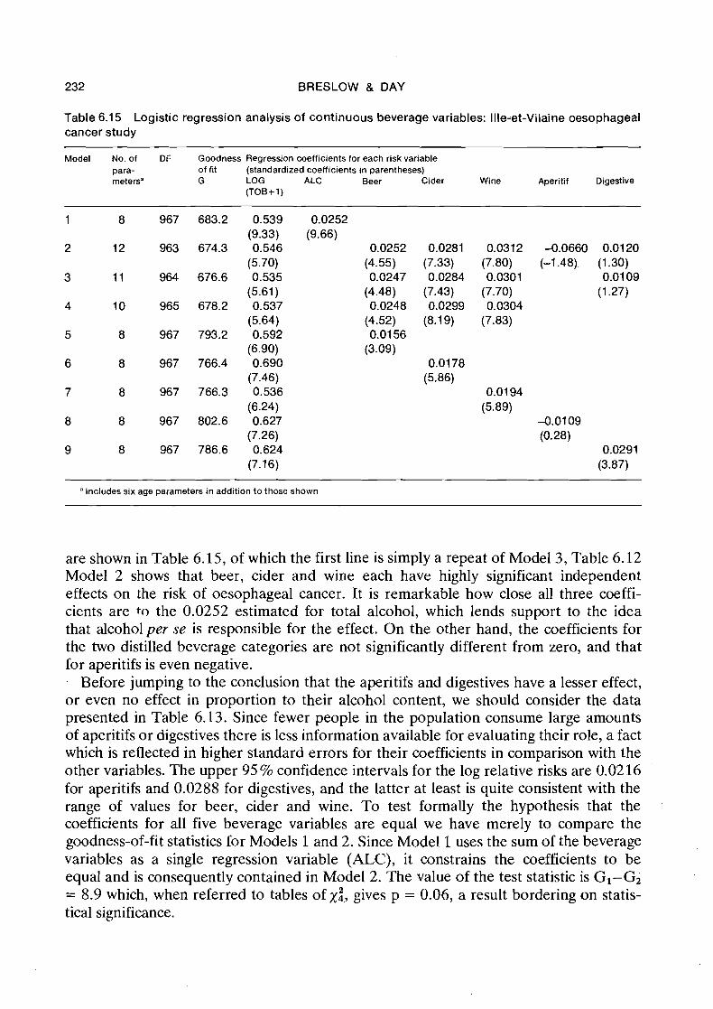
232 BRESLOW & DAY
Table 6.15 Logistic regression analysis of continuous beverage variables: Ille-et-Vilaine oesophageal cancer study
Model No. of DF Goodness Regression coefficients for each risk variable para- of fit (standardized coefficients in parentheses) metersa G LOG ALC Beer Cider Wine Aperitif Digestive
(TOB+1)
a Includes six age parameters in addition to those shown
are shown in Table 6.15, of which the first line is simply a repeat of Model 3, Table 6.12 Model 2 shows that beer, cider and wine each have highly significant independent effects on the risk of oesophageal cancer. It is remarkable how close all three coeffi- cients are to the 0.0252 estimated for total alcohol, which lends support to the idea that alcohol per se is responsible for the effect. On the other hand, the coefficients for the two distilled beverage categories are not significantly different from zero, and that for aperitifs is even negative.
Before jumping to the conclusion that the aperitifs and digestives have a lesser effect, or even no effect in proportion to their alcohol content, we should consider the data presented in Table 6.13. Since fewer people in the population consume large amounts of aperitifs or digestives there is less information available for evaluating their role, a fact which is reflected in higher standard errors for their coefficients in comparison with the other variables. The upper 95 % confidence intervals for the log relative risks are 0.02 16 for aperitifs and 0.0288 for digestives, and the latter at least is quite consistent with the range of values for beer, cider and wine. To test formally the hypothesis that the coefficients for all five beverage variables are equal we have merely to compare the goodness-of-fit statistics for Models 1 and 2. Since Model 1 uses the sum of the beverage variables as a single regression variable (ALC), it constrains the coefficients to be equal and is consequently contained in Model 2. The value of the test statistic is GI-G2 = 8.9 which, when referred to tables of xi, gives p = 0.06, a result bordering on statis- tical significance.
LOGISTIC REGRESSION FOR LARGE STRATA 233
To go one step further we can partition the value into single degree of freedom components by considering two intermediate models: lA, in which the coefficients for beer, cider and wine only were assumed equal; and lB, in which all coefficients were assumed equal except for aperitifs. These yield goodness-of-fit statistics of GIA = 678.9 and GIB = 675.3. Hence we may write G1 - G2 = (GI - GIA) + (GIA - GIB) + (GI,-G2), i.e., 8.9 = 4.3 + 3.6 + 1.0, partitioning the statistic into two x:'s and one ~ 2 . The first, GI-GIA, tests whether aperitifs have an effect different from the average of the remaining beverages (p = 0.04); the second, GIA - GIB, whether digestives differ from the remaining three (p = 0.06); and the last, GIB-G2, tests for differences among the coefficients of beer, cider and wine (p = 0.60). But, since the particular partitioning was suggested by the data rather than from a priori considera- tions, we are faced with a multiple comparisons dilemma and should discount the observed p values.
In the last analysis the situation is somewhat ambiguous. While digestives appear to have lesser effects than the other variables, and aperitifs no effect at all, we cannot rule out at conventional levels of statistical significance the possibility that all beverages contribute to the risk in proportion to their alcohol content.
6.10 Interpretation of regression coefficients
The preceding example considered a model with 12 independent parameters, each of which had a reasonably clear and straightforward interpretation. Six of the para- meters, the a's attached to the six'age strata, were included only to account for possible confounding effects of age. Since age effects were not of special interest, their estimates were not even presented in Table 6.15. However, the controls were obtained as a reasonably random sample of the adult male population so that differences between the a's could be interpreted in terms of log relative risks for the corresponding age groups. (From the a coefficients in Table 6.2, for example, it appears that risk does not change much with age beyond 55 years.) On the other hand, had the sample been stratified by design on the basis of age, no meaning at all could be attached to the a parameters since the effects of age on risk would then be completely confounded with the sampling fractions for different ages (§ 6.3).
While there is generally little interest in the actual values taken on by the a estimates, apart from knowing that the variables they represent have been "accounted for", this is hardly true for the B's. These we have repeatedly interpreted as indicating the change in risk associated with changes in the corresponding regression variables. It is a little disconcerting, therefore, to realize that the estimated regression coefficients may change drastically according to what other variables are included in the model. Such changes are to be anticipated whenever there is collinearity among the regression variables, meaning simply that their,values tend to be correlated in the sampled data. Mosteller and Tukey (1977) provide a good discussion of this problem, which is fundamental to all regression models. Here we consider a few of the main issues, mostly by means of example.
In the Ille-et-Vilaine data there was a remarkable lack of collinearity among age and the levels of consumption of tobacco and total alcohol (Table 4.2). Consequently the estimated relative risks associated with each of these factors were little affected by
234 BRESLOW & DAY
which others were accounted for in the equation. For example, the (age-adjusted) relative risks for the four alcohol categories were 1.0, 4.2, 7.4 and 39.7 without inclu- sion of tobacco in the analysis, and 1.0,4.2, 7.2 and 36.6 with such inc,lusion (Table 6.6).
A better illustration of the effects of collinearity is provided by the analyses of the contributions of individual alcoholic beverages (Table 6.15). We note first that neither the coefficients nor the standard errors of beer, cider and wine are much affected by the presence or absence of aperitif or digestive in the equation (Models 2 4 ) , provided all three of .the alcoholic beverages with significant effects are included. One would anticipate such a result if either (1) there was no correlation between the beverage variables, or (2) aperitif and digestive had no effect on risk beyond that explained by such a correlation (§ 3.4). However, when any one of beer, cider or wine is used as the only alcohol variable (Models 5-7), its coefficient and degree of statistical significance are noticeably reduced. This reflects the fact that cider is negatively correlated with both wine (Q = -0.27) and beer (Q = -0.16). Since an individual consuming a large amount of cider tends to consume less than the average amount of'the other beverages, his apparent cancer risk relative to someone who drinks no cider is reduced unless the effects of these other beverage variables are accounted for by inclusion in the equation.
A different type of change occurs when digestive is used as the only alcohol variable (Model 9). Here the coefficient increases markedly from its value when all alcoholic beverage variables are included, and attains an apparently high level of statistical significance. The explanation now is the positive correlation of digestive with cider (Q = 0.31), such that when cider is not included in the equation, digestive serves, at least partially, as a proxy for its effects. After accounting for the effects of cider the coeffi- cient for digestive falls to a non-significant level. On the other hand, since the correla- tions of digestive with beer and wine are essentially zero (Table 6.14), one would not expect the digestive coefficient to be much altered by the presence of these latter two variables.
Collinearity is bound to arise when both a variable and its square are included in the same equation. Compare, for example, Model 3 with Model 7 in Table 6.12. Introduc- tion of the square term in LOG(T0B + 1) results in an almost doubling of the coeffi- cient for the linear term, from 0.539 to 0.965. At the same time the standardized value decreases, from 9.33 to 3.05, indicating a roughly sixfold increase in the standard error. This is true in spite of the fact that the coefficient of the added variable, L O G 2 ( ~ O ~ + I) , is not statistically significant at all. Indeed, if we were to evaluate the significance of the tobacco effect only on the basis of the standardized coefficients in the quadratic model, we would be sorely misled. The significance of the trend in risk with increased tobacco consumption is well expressed by the single linear term in Model 3; and the large standard errors for LOG(TOB+ 1) and LOG"TOB+ 1) in Model 7 tell us not that these variables are unimportant, but rather that there are many different sets of coefficients for them which express more or less equally well the relationship found in the data. This example illustrates that there is little point in trying to interpret individual coefficients and standard errors in a polynomial regression. A plot of the fitted relation- ship over the range of the regression variables conveys a much more accurate impres- sion of what the equation means.
A similar type of artificial association can arise between one variable representing the main effects of a factor and others representing its interactions, at least if care is not
LOGISTIC REGRESSION FOR LARGE STRATA 235
taken in how these interactions are coded. For example, in order to investigate the interaction between age and alcohol we added to Model 3 of Table 6.12 a variable ALC x AGEGRP, where AGEGRP took on the values 1 to 6 of the age group. Al- though this improved the goodness of fit only slightly, from G = 683.2 to G = 682.1, and the interaction terms had a non-significant regression coefficient, its inclusion in the equation markedly affected the coefficient of ALC. The estimated regression equation (ignoring age effects) changed from
0.0252 ALC + 0.539 LOG(TOB+ 1) (9.66) (9.33)
0.0348ALC + 0.536LOG(TOB+ 1) - 0.00246ALC x AGEGRP, (3.5 8) (5.76) (-1.04)
and by comparing the standardized coefficients (shown in parentheses), we see that the standard error of ALC increased from 0.00261 to 0.00972. Again the explanation is the high degree of collinearity between ALC and ALCx AGEGRP, which can be substantially reduced by subtracting from AGEGRP its modal value of 4 before multi- plying. This leads to an equation
which represents exactly the same relationship as the previous one. However, because the main effect and interaction variables have been coded to reduce the correlation between them, the changes in the coefficient and standard error of the main effect variable are much reduced. Routine coding of interaction or cross-product variables by subtracting mean or modal values from their component parts before multiplying is recommended to avoid the anomalies provoked by such artificial collinearity.
A less artificial example of high correlation between two regression variables occurs when both are measuring the same fundamental quantity in a somewhat imperfect way. In attempting to relate arsenic exposure to cancer risk, for example, we might determine the arsenic concentration of both fingernails and hair of cases and controls, and use each as an indicator of chronic exposure. If these two measures turned out to be highly correlated, as they would if both were good indicators of long-term exposure, it would make little sense to attempt to evaluate their separate effects on risk by including them both in the regression equation. Instead we would take an average or composite of the two values as a single measure of arsenic exposure, and use this along with variables representing other risk factors.
Of course in some problems the collinearity between regression variables will reflect a real association between the corresponding risk factors in the population. While regres- sion analysis is the most powerful tool available for separating out the independent associations with risk, unambiguous answers are simply not possible when collinearity is high. In some cases a judgement as to which is the proper variable, or which risk factor is more likely to play a causal role, will dictate which variables to leave in the
236 BRESLOW & DAY
equation. If such a judgement cannot be made, one must simply admit that precise identification of the factor responsible for the effect is impossible. To quote from Mosteller and Tukey (1977): "We must be prepared for one variable to serve as a proxy for another and worry about the possible consequences, in particular, whether the proxy's coefficient siphons off some of the coefficient we would like to have on the proper variable, or whether a variable serves well only because it is a proxy. In either case, interpretation of the regression coefficient requires very considerable care." Much of the discussion in 5 3.4 on whether or not one should adjust for apparent con- founding variables is relevant here.
6.11 Transforming continuous risk variables
One of the more perplexing issues facing the analyst who uses quantitative regres- sion methods is the choice of appropriate scales on which to express continuous risk variables. He must decide between original measurements, as recorded by machine or interviewer, and such transforms as logs, square roots, reciprocals, or any number of other possibilities. Since the object is to achieve a near-linear relationship between the quantitative regression variable and log risk, it usually helps to make some plots of relative risks for grouped data as we did in Figures 6.1 to 6.4. If the data are sufficiently extensive, so that a regular pattern emerges, one can at least rule out some of the possible choices on the grounds of lack of fit. For example it was fairly clear from both graphical and quantitative analysis of the Ille-et-Vilaine data that the effects of alcohol were best expressed on the original linear scale, while for tobacco a log transform was required.
However epidemiological data are rarely sufficient to enable fine distinctions to be made between rather similar functional forms for the dose-response relationship on statistical grounds alone. Accurate measurements of human exposure to potential risk factors are not often available. Hence recourse is made to animal experimentation for elucidating fundamental aspects of the carcinogenic process. Such experiments allow one to control fairly strictly the amounts of carcinogen administered to homogenous subgroups of animals, and data derived from them are more amenable to precise quanti- tative analysis than are data from observational studies of human populations.
Example: One animal model which has been used to suggest relationships for human epithelial tumours is that of skin-painting experiments in mice. In an experiment reported by Lee and O'Neill (1971), mice were randomly assigned to four dosage groups each containing 300 animals. Starting at about three weeks of age, benzo[alpyrene (BP) was painted on their shaved backs in the following dosages:
Group 1 6 p g BP/week Group 2 1 2 p g BP/week Group 3 24 p g BP/week Group 4 4 8 p g BPlweek
The animals were examined regularly, and the week of tumour occurrence was taken to be the first week that a skin tumour was observed. Age-specific incidence rates of skin tumours were estimated for each dosage group according to the methods of § 2.1. The number of animals developing a skin tumour for the first time during any one week was divided by the number still alive and free of skin tumours a t the middle of that week. Since few new tumours would arise in any given week, these age-specific estimates tended t o be highly unstable. Consequently, the four dosage groups were compared in terms of the age-specific cumulative incidence rates (5 2.3).
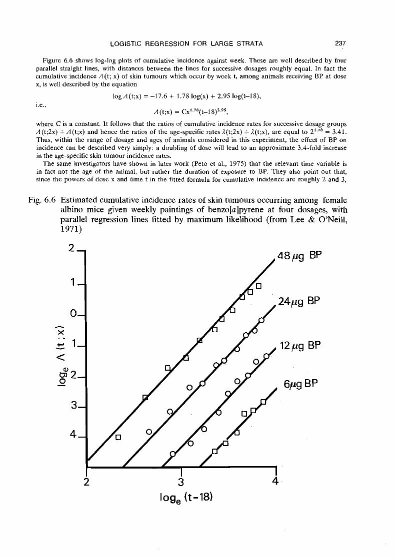
LOGISTIC REGRESSION FOR LARGE STRATA 237
Figure 6.6 shows log-log plots of cumulative incidence against week. These are well described by four parallel straight lines, with distances between the lines for successive dosages roughly equal. In fact the cumulative incidence A(t; x) of skin tumours which occur by week t, among animals receiving BP at dose x, is well described by the equation
log A(t;x) = -17.6 + 1.78 log(x) + 2.95 log(t-18),
A (t;x) = C~' .~ ' ( t - l 8)2.95,
where C is a constant. It follows that the ratios of cumulative incidence rates for successive dosage groups A(t;2x) +- A(t;x) and hence the ratios of the age-specific rates A(t;2x) +- A(t;x), are equal to 21.78 = 3.41. Thus, within the range of dosage and ages of animals considered in this experiment, the effect of BP on incidence can be described very simply: a doubling of dose will lead to an approximate 3.4-fold increase in the age-specific skin tumour incidence rates.
The same investigators have shown in later work (Peto e t al., 1975) that the relevant time variable is in fact not the age of the animal, but rather the duration of exposure to BP. They also point out that, since the powers of dose x and time t in the fitted formula for cumulative incidence are roughly 2 and 3,
Fig. 6.6 Estimated cumulative incidence rates of skin tumours occurring among female albino mice given weekly paintings of benzo[a]pyrene at four dosages, with parallel regression lines fitted by maximum likelihood (from Lee & O'Neill, 1971)
2 3 4 log, (t-18)
238 BRESLOW & DAY
respectively, the data are consistent with a multi-stage theory for the origin of cancer wherein two of the three stages are affected by the carcinogen (Peto, 1977). Recent data for cigarette smoking and lung cancer in the British doctor study likewise suggest that incidence is proportional to the square of the dose rate (Doll & Peto, 1978).
If the linear logistic model were to be used to represent the data in the above ex- periment, this would take the form
for the probability that an animal treated with x units of BP who is still at risk at age ti develops a skin tumour within that week. The ai parameters in turn could be modelled ai = a + y log(ti) as a linear function of log age. There is no problem here with the fact that .the logarithm of a zero dose is - and thus the estimated probability of tumour development 0, since skin tumours do not appear spontaneously on the backs of mice without treatment. For other studies, especially with humans, one could sub- stitute a dose metameter of the form z = log(x+ xo), where x was the measured dose while xo represented a small background dose which was presumably responsible for any spontaneous cases. Although in principle it is possible to estimate xo from the data by maximum likelihood, this is rarely done. Special programmes would be required for such estimation since xo does not enter the regression equation in the same linear fashion as the other parameters. Furthermore, since different combinations of xo and /? can give virtually identical fits to the data, the standard errors and covariances for the jointly estimated parameters tend to be large. Hence the best practice may simply be to assign xo some small value on the basis of a priori considerations. With the Ille-et- Vilaine tobacco data, we set xo = 1 and noticed that the resulting curve seemed to fit the observed data reasonably well (Figure 6.5).
6.12 Studies of interaction in a series of 2 x 2 tables
One of the principal advantages of using the logistic regression model is that it encourages quantitative description of how the changes in risk associated with one factor are modified by the interaction effects of other risk or nuisance variables. Since the Ille-et-Vilaine data are notably lacking in such interactions, they cannot be used to illustrate this important feature of statistical modelling. Hence in this section we analyse another set of published data, which happen to be in the form of a series of 2 x 2 tables, for which strong interaction effects are present.
Presence of interaction effects in a. series of 2 x 2 tables means that the odds ratios depend systematically on the variables used for strata formation. Such dependence may have important implications for the nature of the disease process. The data we shall consider are those of Stewart and Kneale (1970) who hypothesized that the distribution of age at diagnosis for childhood cancers caused by obstetric X-rays was more concentrated or "peaked" than the age distribution of idiopathic childhood cancers. If this were so the risk ratio for irradiated versus non-irradiated children would also show a peak when plotted against age. The effect would presumably occur because the time of exposure for the radiogenic cases is limited to the period of gestation, while for other cancers it could vary over a broader age span.
LOGISTIC REGRESSION FOR LARGE STRATA 239
Such variations are detected by the addition of interaction terms to the logistic model. In 5 6.5 we considered a model in which the log relative risk was assumed to change linearly over the six age strata. More generally one might define several dif- ferent regression variables, including tra.nsformations and cross-product terms, from factors such as age and time which are used to define strata. Let us denote by zil the value of the lth variable for the ith stratum (i = 1, .. ., I; 1 = 1, ..., L). Then the inter- action model may be written
where as usual Pi(x) denotes the disease probability in the ith stratum for an exposed (x = 1) or unexposed (x = 0) individual. A consequence of this formulation is that the log relative risk for the ith stratum is expressed
pi(1 )Qi(o) L log 7# = log pi(o)Qi(l)
= P + I= 2 1 ~lzil
as a linear function of the regression variables z, with the "constant" term P denoting the baseline log relative risk for the group having covariate values z = 0. It is best to code the covariates in such a way that z = 0 corresponds to some "typical" individual.
Summary data from the Oxford Childhood Cancer Survey and associated studies reported by Kneale (1971) are presented in Appendix 11. Cases were ascertained as all children under ten years of age in England and Wales who died of cancer (leukaemia or solid tumours) during the period 1954-65. For each of these a neighbourhood control of the same age was selected who was alive and well at the time the case died. Only "traced" pairs, for whom both case and control mothers could be found and interviewed, were analysed. The published data ignore the exact pairing but do preserve the stratification by age and year of birth.
Exposure in this example is simply a question of whether or not the study subjects received in utero irradiation, as reported by the mother. The stratification variables were age at death, from 0 to 9 years, and year of birth, from 1944 to 1964. Because of the limited period of case ascertainment, not all 210 possible combinations of these factors appear. For example, among childhood cancer patients born in 1944, only those who died at age 9 are represented. A total of 120 such strata were available.
In order to estimate the overall relative risk of obstetric radiation, and to determine whether, and if so how, it varied with age and year, we fitted several versions of the model (6.25). Five different regression variables were used: zl = year of birth, coded zl = -10 for 1944, . . ., z1 = 10 for 1964; z, = z: -22; z, = age at death, coded -9 for age 0, -7 for age 1, . .., 9 for age 9; ~q = z i -33; and z, = z, x z,. Different subsets of these were entered into the regression equation so as to detect particular kinds of trends and patterns in the relative risk.
Results of the analysis are shown in Table 6.16. Degrees of freedom (DF) for each model were obtained in the usual manner by subtracting the number of parameters, in this case the 120 a's plus additional P and y terms, from the number of binomial observations, namely 240. The first model, which includes only the a's, assumes that the relative risk is unity in each stratum. In view of the large goodness-of-fit statistics, this supposition is clearly untenable. The second model specifies a constant relative
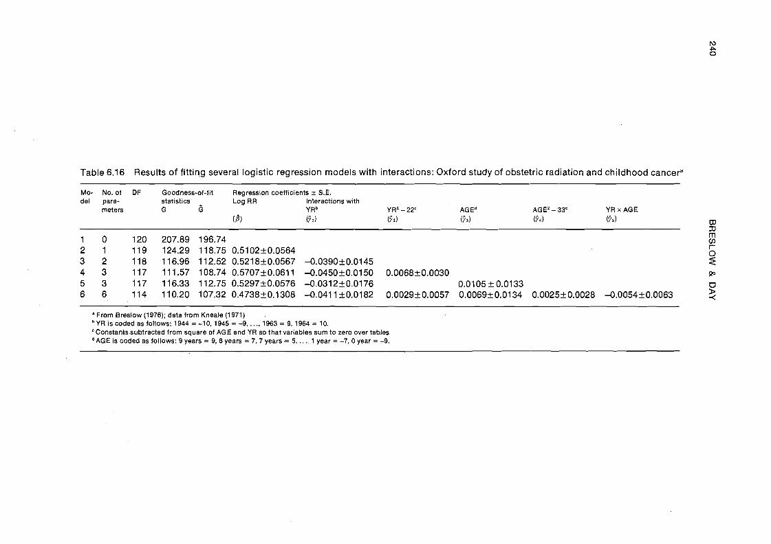
Table 6.16 Results of fitting several logistic regression models with interactions: Oxford study of obstetric radiation and childhood cancera -
Mo- No. of DF Goodness-of-fit Regression coefficients 2 S.E. del para- statistics Log RR Interactions with
meters G 6 YRb YR2 - 22' AGEd AGEZ - 33' YR x AGE
'From Breslow (1976); data from Kneale (1971) YR is coded as follows: 1944 = -10, 1945 = -9, . . ., 1963 = 9. 1964 = 10. Constants-subtracted from square of AGE and YR so that variables sum to zero over tables
dAGE is coded as follows: 9 years = 9, 8 years = 7,7 years = 5, . . ., 1 year = -7,0 year = -9.
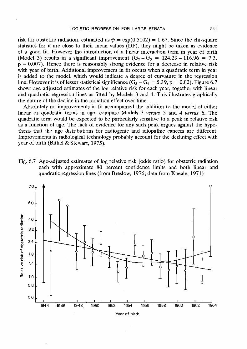
LOGISTIC REGRESSION FOR LARGE STRATA 241
risk for obstetric radiation, estimated as $ = exp(0.5102) = 1.67. Since the chi-square statistics for it are close to their mean values (DF), they might be taken as evidence of a good fit. However the introduction of a linear interaction term in year of birth (Model 3) results in a significant improvement (G2 - G3 = 124.29 - 1 16.96 = 7.3, p = 0.007). Hence there is reasonably strong evidence for a decrease in relative risk with year of birth. Additional improvement in fit occurs when a quadratic term in year is added to the model, which would indicate a degree of curvature in the regression line. However it is of lesser statistical significance (G3 - G4 = 5.39, p = 0.02). Figure 6.7 shows age-adjusted estimates of the log-relative risk for each year, together with linear and quadratic regression lines as fitted by Models 3 and 4. This illustrates graphically the nature of the decline in the radiation effect over time.
Absolutely no improvements in fit accompanied the addition to the model of either linear or quadratic terms in age: compare Models 3 versus 5 and 4 versus 6. The quadratic term would be expected to be particularly sensitive to a peak in relative risk as a function of age. The lack of evidence for any such peak argues against the hypo- thesis that the age distributions for radiogenic and idiopathic cancers are different. Improvements in radiological technology probably account for the declining effect with year of birth (Bithel & Stewart, 1975).
Fig. 6.7 Age-adjusted estimates of log relative risk (odds ratio) for obstetric radiation each with approximate 80 percent confidence limits and both linear and quadratic regression lines (from Breslow, 1976; data from Kneale, 1971)
Year of birth
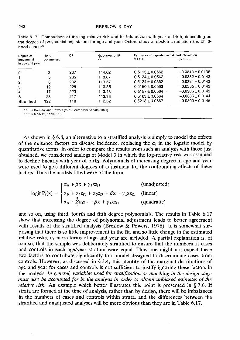
242 BRESLOW & DAY
Table 6.17 Comparison of the log relative risk and its interaction with year of birth, depending on the degree of polynomial adjustment for age and year: Oxford study of obstetric radiation and child- hood cancera
Degree of No. of D F Goodness of fit Estimates of log-relative risk and interaction polynomial parameters 6 f l ? S.E. p, 2 S.E. in age and year
a From Breslow and Powers (1978); data from Kneale (1971) From Model 3, Table 6.16
As shown in 3 6.8, an alternative to a stratified analysis is simply to model the effects of the nuisance factors on disease incidence, replacing the ai in the logistic model by quantitative terms. In order to compare the results from such an analysis with those just obtained, we considered analogs of Model 3 in which the log-relative risk was assumed to decline linearly with year of birth. Polynomials of increasing degree in age and year were used to give different degrees of adjustment for the confounding effects of these factors. Thus the models fitted were of the form
a o + px + ylxzil (unadjusted)
logit Pi(x) = a. + alzil + a3zi3 + px + ylxzil (linear) 6
a. + Talzil + px + ylxzil (quadratic)
and so on, using third, fourth and fifth degree polynomials. The results in Table 6.17 show that increasing the degree of polynomial adjustment leads to better agreement with results of the stratified analysis (Breslow & Powers, 1978). It is somewhat sur- prising that there is so little improvement in the fit, and so little change in the estimated relative risks, as more terms of age and year are included. A partial explanation is, of course, that the sample was deliberately stratified to ensure that the numbers of cases and controls in each age/year stratum were equal. Thus one might not expect these two factors to contribute significantly to a model designed to discriminate cases from controls. However, as discussed in 5 3.4, this identity of the marginal distributions of age and year for cases and controls is not sufficient to justify ignoring these factors in the analysis. In general, variables used for stratification or matching in the design stage must also be accounted for in the analysis in order to obtain unbiased estimates of the relative risk. An example which better illustrates this point is presented in 5 7.6. If strata are formed at the time of analysis, rather than by design, there will be imbalances in the numbers of cases and controls within strata, and the differences between the stratified and unadjusted analyses will be more obvious than they are in Table 6.17.
LOGISTIC REGRESSION FOR LARGE STRATA
REFERENCES
Anderson, J. A. (1972) Separate sample logistic discrimination. Bwmetrika, 59, 19-35 Armitage, P. (1975) Statistical Methods in Medical Research, Oxford, Blackwell Baker, R.J. & Nelder, J.A. (1978) The GLIM System. Release 3, Oxford, Numerical
Algorithms Group Bishop, Y. M.M., Fienberg, S. E. & Holland, P. W. (1975) Discrete Multivariate Analysis:
Theory and Practice, Cambridge, Mass., MIT Press Bithel, J. & Stewart, A. (1975) Pre-natal irradiation and childhood malignancy: a review
of British data from the Oxford Survey. Br. J. Cancer, 31, 271-287 Breslow, N. E. (1975) Analysis of survival data under the proportional hazards model.
Rev. Int. Stat., 43, 45-58 Breslow, N. E. (1976) Regression analysis of the log odds ratio: a method for retrospective
studies. Biometries, 32, 4 0 9 4 16 Breslow, N. E. (1978) The proportional hazards model: applications in epidemiology.
Comm. Stat.-Theor. Meth., A7, 3 15-332 Breslow, N. E., Day, N. E., Halvorsen, K.T., Prentice, R.L. & Sabai, C. (1978) Estima-
tion of multiple relative risk functions in matched case-control studies. Am. J. Epi- demiol., 108, 299-307
Breslow, N . E. & Powers, W. (1978) Are there two logistic regressions for retrospective studies? Biometrics, 34, 100-105
Cornfield, J. (1962) Joint dependence of the risk of coronary heart disease on serum cholesterol and systolic blood pressure: a discriminant function analysis. Fed. Proc., 21, 58-61
Cox, D. R. (1 970) The Analysis of Binary Data, London, Methuen Cox, D.R. (1972) Regression models and life tables (with discussion). J. R. stat.
SOC. B, 34, 187-220 Cox, D. R. & Hinkley, D. V. (1 974) Theoretical Statistics, London, Chapman & Hall Day, N. E. & Byar, D. P. (1979) Testing hypotheses in case-control studies - equivalence
of Mantel-Haenszel statistics and logit score tests. Biometries, 35, 623-630 Day, N. E. & Kerridge, D.F. (1967) A general maximum likelihood discriminant. Bio-
metries, 23, 3 13-323 Doll, R. & Peto, R. (1978) Cigarette smoking and bronchial carcinoma: dose and time
relationships among regular smokers and lifelong non-smokers. J. Epidemiol. Com- munity Health, 32, 303-3 13
Efron, B. (1975) The efficiency of logistic regression compared to normal theory discriminant analysis. J. Am. stat. Assoc., 70, 892-898
Farewell, V.T. (1979) Some results on the estimation of logistic models based on retrospective data. Biometrika, 66, 27-32
Fienberg, S. E. (1977) The Analysis of Cross-Classified Data, Cambridge, Mass., MIT Press
Haberman, S.J. (1974) The Analysis of Frequency Data, Chicago, University of Chi- cago Press
Halperin, M., Blackwelder, W.C. & Verter, J. I. (1971) Estimation of the multivariate logistic risk function: a comparison of the discriminant function and maximum likeli- hood approaches. J. chron. Dis., 24, 125-158
244 BRESLOW & DAY
Kneale, G. W. (1971) Problems arising in estimating from retrospective survey data the latent period of juvenile cancers initiated by obstetric radiography. Biometrics, 27, 563-590
Lee, P. & O'Neill, J. (1971) The effect of both time and dose on tumour incidence rate in benzopyrene skin painting experiments. Br. J. Cancer, 25, 759-770
Lininger, L., Gail, M., Green, S. & Byar, D. (1979) Comparison of four tests for equality of survival curves in the presence of stratification and censoring. Biometrika, 63, 419-428
Mantel, N. (1973) Synthetic retrospective studies and related topics. Biometrics, 29, 479-486
Mosteller, F . & Tukey, J.W. (1977) Data Analysis and Regression: a Second Course in Statistics, Reading, Mass., Addison & Wesley
Nelder, J.A. (1977) A reformulation of linear models. J. R. stat. Soc. A, 140, 48-77 Peto, R. (1977) Epidemiology, multistage models and short-term mutagenicity tests.
In: Hiatt, H. H., Watson, J. D. & Winsten, J. A., eds. Origins of Human Cancer, Cold Spring Harbor, NY, Cold Spring Harbor Publications, Vol. 4, pp. 1403-1421
Peto, R., Roe, F., Lee, P., Levy, L. & Clark, J. (1975) Cancer and ageing in mice and men. Br. J. Cancer, 32, 4 11-426
Prentice, R.L. & Breslow, N.E. (1978) Retrospective studies and failure time models. Biometrika, 65, 153-1 58
Prentice, R.L. & Pyke, R. (1979) Logistic disease incidence models and case-control studies. Biometrika, 66, 403-4 1 1
Press, S. J. & Wilson, S. (1978) Choosing between logistic regression and discriminant analysis. J. Am. stat. Assoc., 70, 699-705
Rao, C. R. (1965) Linear Statistical Inference and its Applications, New York, Wiley Seigel, D. G. & Greenhouse, S. W. (1973) Multiple relative risk functions in case-control
studies. Am. J. Epidemiol., 97, 324-331 Stewart, A. & Kneale, G.W. (1970) Age-distribution of cancers caused by obstetric
x-rays and their relevance to cancer latent periods. Lancet, ii, 4-8 Thomson, W.A., Jr (1977) On the treatment of grouped observations in life studies
Biometrics, 33, 463-470 Truett, J., Cornfield, J. & Kannel, W. (1967) A multivariate analysis of the risk of
coronary heart disease in Framingham. J. chron. Dk., 20, 51 1-524 Vitaliano, P.O. (1978) The use of logistic regression for modelling risk factors: with
application to non-melanoma skin cancer. Am. J. Epidemiol., 108, 402-414 Walker, S.H. & Duncan, D.B. (1967) Estimation of the probability of an event as a
function of several independent variables. Biometrika, 54, 167-179
LIST OF SYMBOLS - CHAPTER 6 (in order of appearance)
logit(p) P the logistic transform of a proportion p; log(-) 1-P
x risk variable V odds ratio P log odds ratio
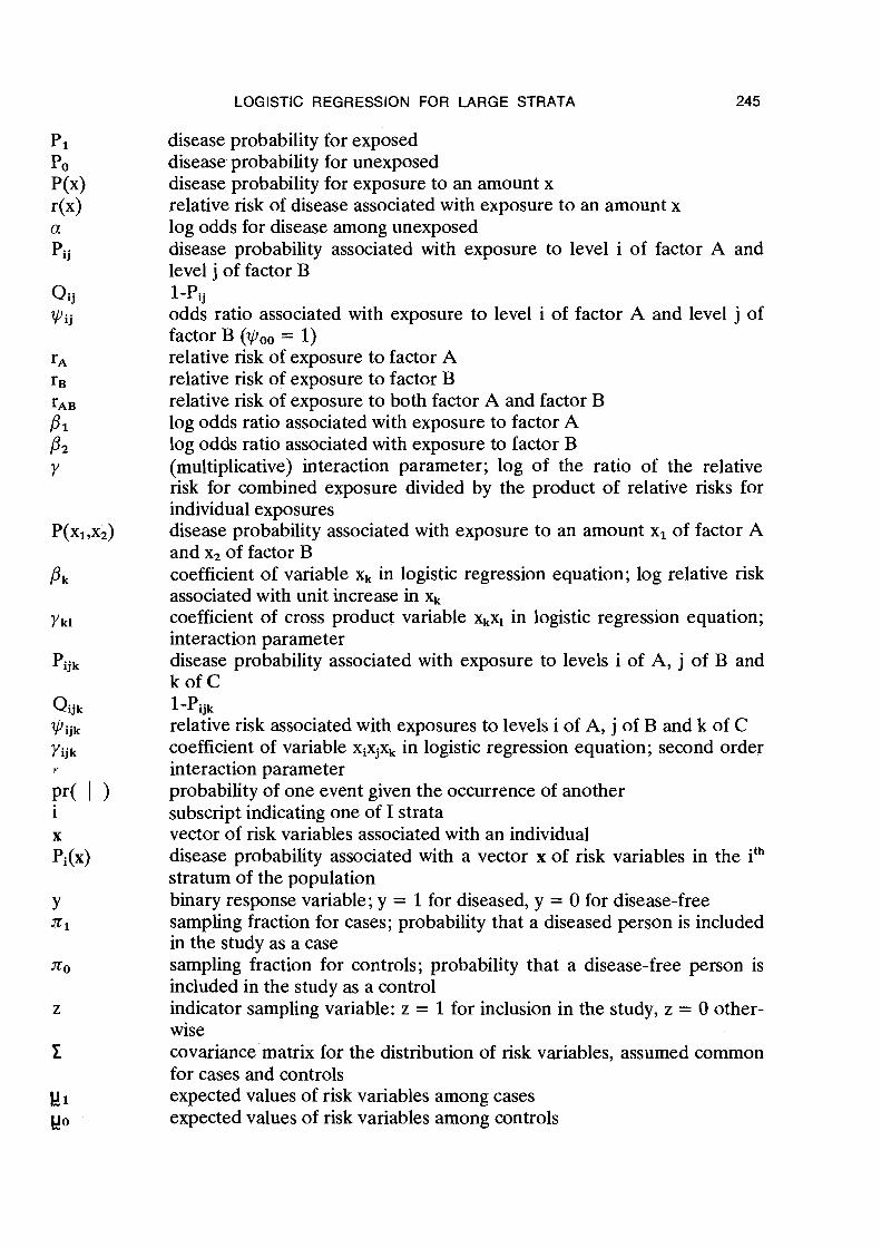
LOGISTIC REGRESSION FOR LARGE STRATA
Qij Wij
disease probability for exposed disease probability for unexposed disease probability for exposure to an amount x relative risk of disease associated with exposure to an amount x log odds for disease among unexposed disease probability associated with exposure to level i of factor A and level j of factor B 1 -P, odds ratio associated with exposure to level i of factor A and level j of factor B (Woo = 1) relative risk of exposure to factor A relative risk of exposure to factor B relative risk of exposure to both factor A and factor B log odds ratio associated with exposure to factor A log odds ratio associated with exposure to factor B (multiplicative) interaction parameter; log of the ratio of the relative risk for combined exposure divided by the product of relative risks for individual exposures disease probability associated with exposure to an amount xl of factor A and x2 of factor B coefficient of variable xk in logistic regression equation; log relative risk associated with unit increase in xk coefficient of cross product variable xkxl in logistic regression equation; interaction parameter disease probability associated with exposure to levels i of A, j of B and k o f C 1 -Pijk relative risk associated with exposures to levels i of A, j of B and k of C coefficient of variable xixjxk in logistic regression equation; second order interaction parameter probability of one event given the occurrence of another subscript indicating one of I strata vector of risk variables associated with an individual disease probability associated with a vector x of risk variables in the ith stratum of the population binary response variable; y = 1 for diseased, y = 0 for disease-free sampling fraction for cases; probability that a diseased person is included in the study as a case sampling fraction for controls; probability that a disease-free person is included in the study as a control indicator sampling variable: z = 1 for inclusion in the study, z = 0 other- wise covariance matrix for the distribution of risk variables, assumed common for cases and controls expected values of risk variables among cases expected values of risk variables among controls
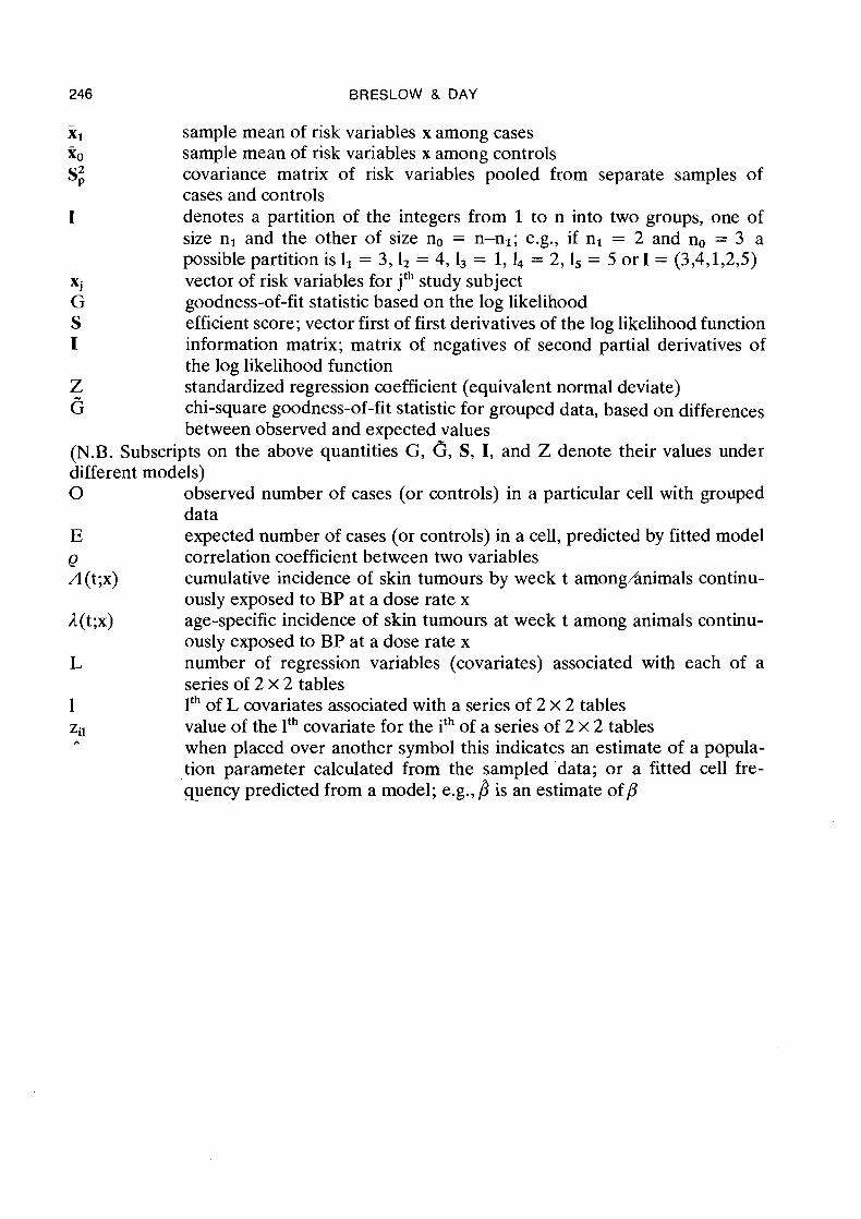
246 BRESLOW & DAY
-
XI sample mean of risk variables x among cases - xo sample mean of risk variables x among controls
s; covariance matrix of risk variables pooled from separate samples of cases and controls
1 denotes a partition of the integers from 1 to n into two groups, one of size nl and the other of size no = n-nl; e.g., if nl = 2 and no = 3 a possible partition is 1, = 3,1, = 4, 1, = 1, = 2,1, = 5 or 1 = (3,4,1,2,5)
Xj vector of risk variables for jth study subject G goodness-of-fit statistic based on the log likelihood S efficient score; vector first of first derivatives of the log likelihood function I information matrix; matrix of negatives of second partial derivatives of
the log likelihood function Z standardized regression coefficient (equivalent normal deviate) (3 chi-square goodness-of-fit statistic for grouped data, based on differences
between observed and expected values (N.B. Subscripts on the above quantities G, G, S, I, and Z denote their values under different models) 0 observed number of cases (or controls) in a particular cell with grouped
data E expected number of cases (or controls) in a cell, predicted by fitted model Q correlation coefficient between two variables A (t;x) cumulative incidence of skin tumours by week t amonghnimals continu-
ously exposed to BP at a dose rate x 1 (t;x) age-specific incidence of skin tumours at week t among animals continu-
ously exposed to BP at a dose rate x L number of regression variables (covariates) associated with each of a
series of 2 x 2 tables 1 lth of L covariates associated with a series of 2 x 2 tables Zil value of the lth covariate for the ith of a series of 2 x 2 tables ,. when placed over another symbol this indicates an estimate of a popula-
tion parameter calculated from the sampled data; or a fitted cell fre- quency predicted from a model; e.g., B is an estimate of @