5. Levels of reliability methods

There are different levels of reliability analysis, which can be used in any design

methodology depending on the importance of the structure. The term 'level' is

characterized by the extent of information about the problem that is used and provided.

The methods of safety analysis proposed currently for the attainment of a given limit state

can be grouped under four basic “levels” (namely levels IV, III, II, and I ) depending

upon the degree of sophistication applied to the treatment of the various problems.

1. In level I methods, the probabilistic aspect of the problem is taken into account by

introducing into the safety analysis suitable “characteristic values” of the random

variables, conceived as fractile of a predefined order of the statistical distributions

concerned. These characteristic values are associated with partial safety factors

that should be deduced from probabilistic considerations so as to ensure

appropriate levels of reliability in the design. In this method, the reliability of the

design deviate from the target value, and the objective is to minimize such an

error. Load and Resistance Factor Design (LRFD) method comes under this

category.

2. Reliability methods, which employ two values of each uncertain parameter (i.e.,

mean and variance), supplemented with a measure of the correlation between

parameters, are classified as level II methods.

3. Level III methods encompass complete analysis of the problem and also involve

integration of the multidimensional joint probability density function of the

1

random variables extended over the safety domain. Reliability is expressed in

terms of suitable safety indices, viz., reliability index, β and failure probabilities.

4. Level IV methods are appropriate for structures that are of major economic

importance, involve the principles of engineering economic analysis under

uncertainty, and consider costs and benefits of construction, maintenance, repair,

consequences of failure, and interest on capital, etc. Foundations for sensitive

projects like nuclear power projects, transmission towers, highway bridges, are

suitable objects of level IV design.

5. 1. Space of State Variables

For analysis, we need to define the state variables of the problem. The state variables are

the basic load and resistance parameters used to formulate the performance function. For

‘n’ state variables, the limit state function is a function of ‘n’ parameters .

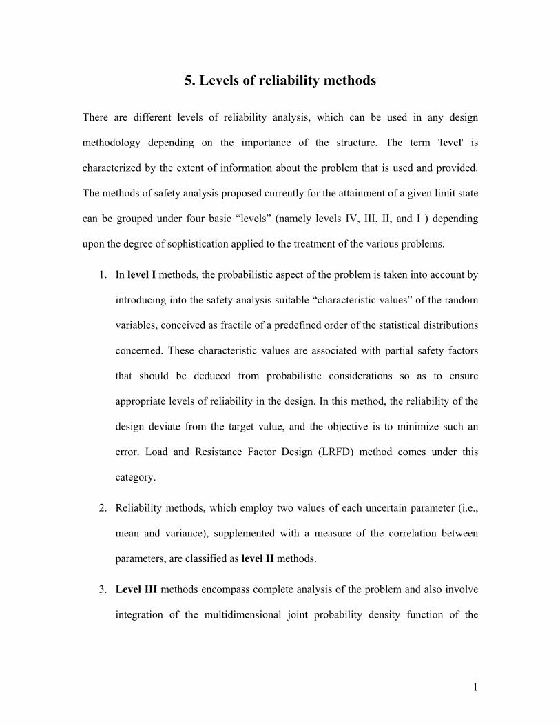
If all loads (or load effects) are represented by the variable Q and total resistance (or

capacity) by R, then the space of state variables is a two-dimensional space as shown in

Figure 1. Within this space, we can separate the “safe domain” from the “failure

domain”; the boundary between the two domains is described by the limit state function

g(R,Q)=0.

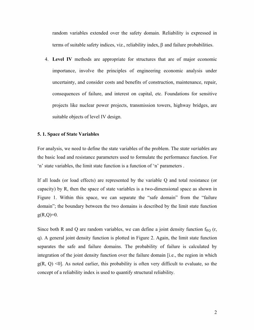
Since both R and Q are random variables, we can define a joint density function fRQ (r,

q). A general joint density function is plotted in Figure 2. Again, the limit state function

separates the safe and failure domains. The probability of failure is calculated by

integration of the joint density function over the failure domain [i.e., the region in which

g(R, Q) <0]. As noted earlier, this probability is often very difficult to evaluate, so the

concept of a reliability index is used to quantify structural reliability.

2

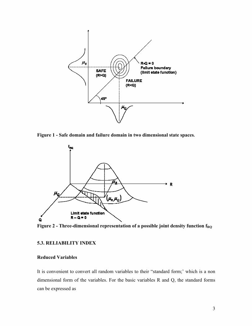
Figure 1 - Safe domain and failure domain in two dimensional state spaces.

Figure 2 - Three-dimensional representation of a possible joint density function fRQ

5.3. RELIABILITY INDEX

Reduced Variables

It is convenient to convert all random variables to their “standard form;’ which is a non

dimensional form of the variables. For the basic variables R and Q, the standard forms

can be expressed as

3

Q

QQ

R

RR

RZ

RZ

σμ

σμ

−=

−=

-------------------------------- (1)

The variables ZR and ZQ, are sometimes called reduced variables. By rearranging

Equation no.1, the resistance R and the load Q can be expressed in terms of the reduced

variables as follows:

QQQ

RRR

ZRZR

σμσμ

+=+=

-------------------------------- (2)

The limit state function g(R, Q) = R-Q can be expressed in terms of the reduced variables

by using Eqs. 2. The result is

QQRRQRQQQRRRQR ZZZZZZg σσμμσμσμ −+−=−−+= )(),( ------------(3)

For any specific value of g(ZR, ZQ), Equation no.3 represents a straight line in the space

reduced variables ZR and ZQ. The line corresponding to g(ZR, ZQ) =0 separates the safe

and failure domain in the space of reduced variables. The loads Q and resistances R are

some times indicated in terms of capacity C and demand D as well in literature.

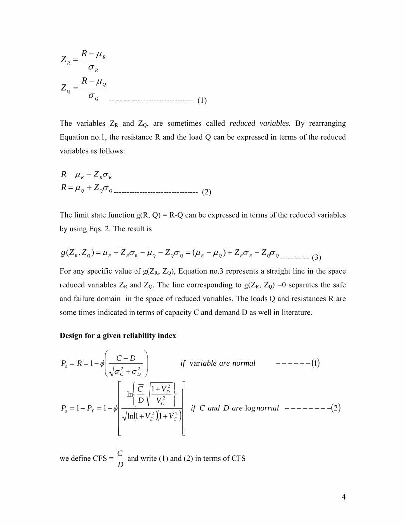
Design for a given reliability index

( )

( )( )( )2log

11ln

1ln

11

1var1

22

2

2

22

−−−−−−−−

⎥⎥⎥⎥⎥⎥

⎦

⎤

⎢⎢⎢⎢⎢⎢

⎣

⎡

++

⎪⎭

⎪⎬⎫

⎪⎩

⎪⎨⎧ +

−=−=

−−−−−−⎟⎟

⎠

⎞

⎜⎜

⎝

⎛

+

−−==

normalareDandCifVV

VV

DC

PP

normalareiableifDCRP

CD

C

D

fs

DC

s

φ

σσφ

we define CFS = DC and write (1) and (2) in terms of CFS

4

( )

( )( )22

2

2

222

11ln

11

ln

1

CD

C

D

DC

VV

VV

CFS

normalareDandCforVVCFS

CFS

++

⎟⎟

⎠

⎞

⎜⎜

⎝

⎛

++

=

+

−=

β

β

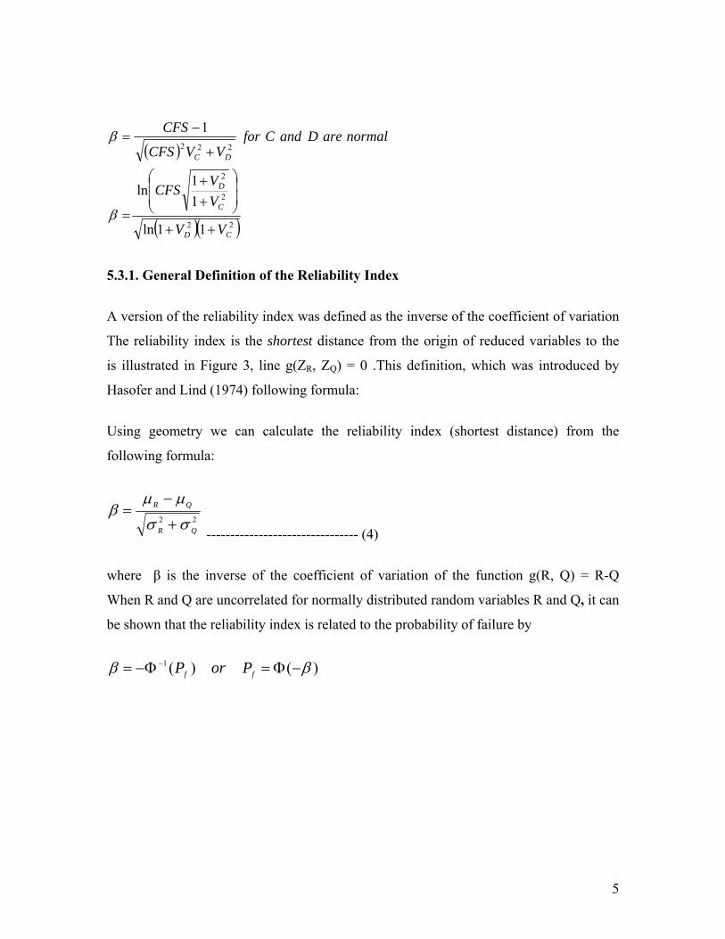
5.3.1. General Definition of the Reliability Index

A version of the reliability index was defined as the inverse of the coefficient of variation

The reliability index is the shortest distance from the origin of reduced variables to the

is illustrated in Figure 3, line g(ZR, ZQ) = 0 .This definition, which was introduced by

Hasofer and Lind (1974) following formula:

Using geometry we can calculate the reliability index (shortest distance) from the

following formula:

22QR

QR

σσ

μμβ

+

−=

-------------------------------- (4)

where β is the inverse of the coefficient of variation of the function g(R, Q) = R-Q

When R and Q are uncorrelated for normally distributed random variables R and Q, it can

be shown that the reliability index is related to the probability of failure by

)()(1 ββ −Φ=Φ−= −ff PorP

5

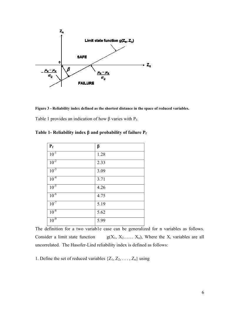
Figure 3 - Reliability index defined as the shortest distance in the space of reduced variables.

Table 1 provides an indication of how β varies with Pf.

Table 1- Reliability index β and probability of failure Pf

Pf β

10-1 1.28

10-2 2.33

10-3 3.09

10-4 3.71

10-5 4.26

10-6 4.75

10-7 5.19

10-8 5.62

10-9 5.99

The definition for a two variab1e case can be generalized for n variables as follows.

Consider a limit state function g(X1, X2…… Xn), Where the Xi variables are all

uncorrelated. The Hasofer-Lind reliability index is defined as follows:

1. Define the set of reduced variables {Z1, Z2, . . . , Zn} using

6

i

i

X

Xii

XZ

σμ−

=--------------------------------(5)

2. Redefine the limit state function by expressing it in terms of the reduced variables

(Z1,Z2,..,,Zn).

3. The reliability index is the shortest distance from the origin in the n-dimensional space

of reduced variables to the curve described by g(Z1, Z2, . . . , Zn) = 0.

5.4. First-order second moment method (FOSM)

This method is also referred to as mean value first-order second moment (MVFOSM)

method, and it is based on the first order Taylor series approximation of the performance

function linearized at the mean values of the random variables. It uses only second-

moment statistics (mean and variance) of the random variables. Originally, Cornell

(1969) used the simple two variable approaches. On the basic assumption that the

resulting probability of Z is a normal distribution, by some relevant virtue of the central

limit theorem, Cornell (1969) defined the reliability index as the ratio of the expected

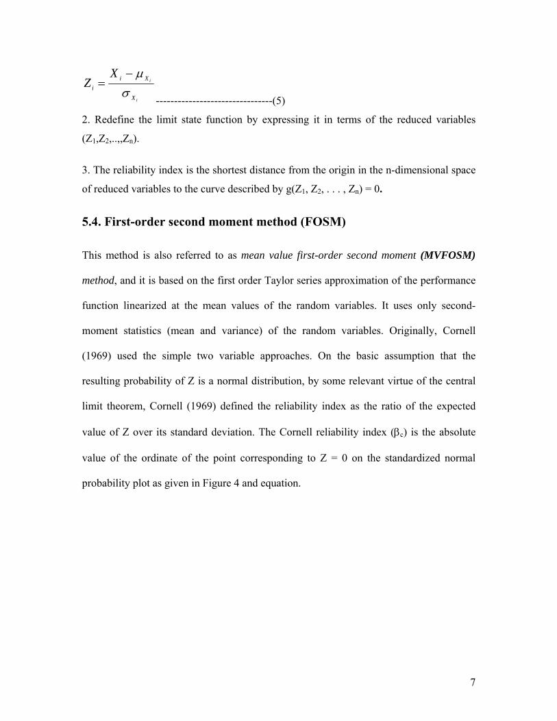
value of Z over its standard deviation. The Cornell reliability index (βc) is the absolute

value of the ordinate of the point corresponding to Z = 0 on the standardized normal

probability plot as given in Figure 4 and equation.

7

μZ

σZ βcLimit surface

z=0

fZ(z)

Figure 4- Definition of limit state and reliability index

22SR

SR

z

zc

σσ

μμσμ

β+

−== -----------------------------------(6)

On the other hand, if the joint probability density function fX(x) is known for the multi

variable case, then the probability of failure pf is given by

∫=L

Xf dXxfp )( -----------------------------------(7)

where L is the domain of X where g(X)<0.

In general, the above integral cannot be solved analytically, and an approximation is

obtained by the FORM approach. In this approach, the general case is approximated to an

ideal situation where X is a vector of independent Gaussian variables with zero mean and

unit standard deviation, and where g(X) is a linear function. The probability of failure pf

is then:

∑ β−Φ=<β−α=<==

n

1iiif )()0X(P)0)X(g(Pp -----------------------------------(8)

8

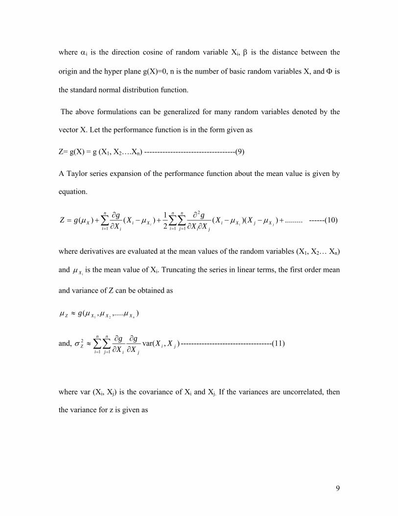
where αi is the direction cosine of random variable Xi, β is the distance between the

origin and the hyper plane g(X)=0, n is the number of basic random variables X, and Φ is

the standard normal distribution function.

The above formulations can be generalized for many random variables denoted by the

vector X. Let the performance function is in the form given as

Z= g(X) = g (X1, X2….Xn) -----------------------------------(9)

A Taylor series expansion of the performance function about the mean value is given by

equation.

∑ ∑∑= = =

+−−∂∂

∂+−

∂∂

+=n

i

n

i

n

jXjXi

jiXi

iX jii

XXXXgX

XggZ

1 1 1

2

.........))((21)()( μμμμ ------(10)

where derivatives are evaluated at the mean values of the random variables (X1, X2… Xn)

and iXμ is the mean value of Xi. Truncating the series in linear terms, the first order mean

and variance of Z can be obtained as

),.....,(21 nXXXZ g μμμμ ≈

and, ∑∑= = ∂

∂∂∂

≈n

i

n

jji

jiZ XX

Xg

Xg

1 1

2 ),var(σ -----------------------------------(11)

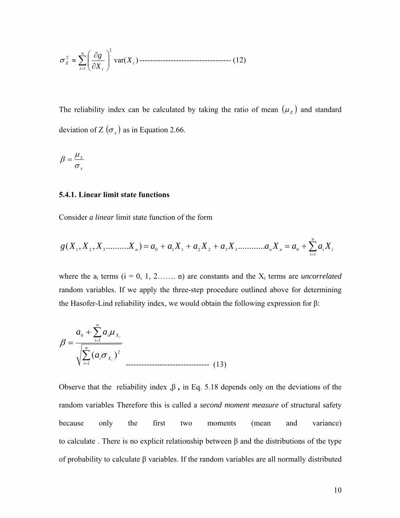
where var (Xi, Xj) is the covariance of Xi and Xj. If the variances are uncorrelated, then

the variance for z is given as

9

∑=

⎟⎟⎠

⎞⎜⎜⎝

⎛∂∂

≈n

ii

iZ X

Xg

1

22 )var(σ ----------------------------------- (12)

The reliability index can be calculated by taking the ratio of mean ( Z )μ and standard

deviation of Z ( z )σ as in Equation 2.66.

z

z

σμ

β =

5.4.1. Linear limit state functions

Consider a linear limit state function of the form

∑=

+=+++=n

iiinnn XaaXaXaXaXaaXXXXg

103322110321 ............)..........,,(

where the ai terms (i = 0, 1, 2……. n) are constants and the Xi terms are uncorrelated

random variables. If we apply the three-step procedure outlined above for determining

the Hasofer-Lind reliability index, we would obtain the following expression for β:

∑

∑

=

=

+=

n

iXi

n

iXi

i

i

a

aa

1

2

10

)( σ

μβ

-------------------------------- (13)

Observe that the reliability index ,β , in Eq. 5.18 depends only on the deviations of the

random variables Therefore this is called a second moment measure of structural safety

because only the first two moments (mean and variance)

to calculate . There is no explicit relationship between β and the distributions of the type

of probability to calculate β variables. If the random variables are all normally distributed

10

and uncorrelated then this formula is exact in the sense that β and Pf are related by Eq.

5.15. Otherwise, Eq. 5.15 Provides only an approximate means of Probability of failure.

The method discussed above has some limitations and deficiencies. It does not use the

distribution information about the variable and function g( ) is linearized at the mean

values of the Xi variables. If g( ) is non-linear, neglecting of higher order term in Taylor

series expansion introduces significant error in the calculation of reliability index. The

more important observation is that the Equations 2.58 and 2.64 do not give constant value

of reliability index for mechanically equivalent formulations of the same performance

function. For example, safety margin R-S<0 and R/S <1 are mechanically equivalent yet

these safety margins will not lead to same value of probability of failure. Moreover,

MVFOSM approach does not use the distribution information about the variables when it

is available.

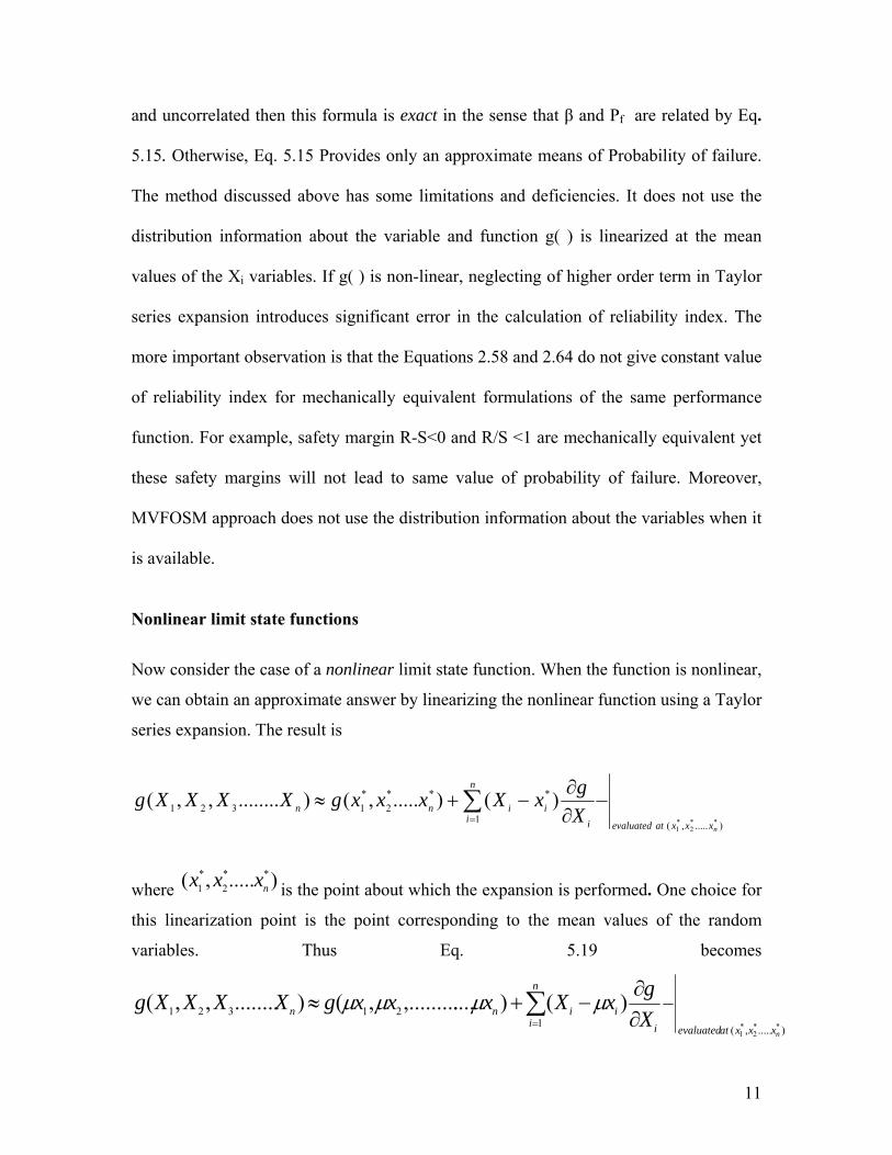
Nonlinear limit state functions

Now consider the case of a nonlinear limit state function. When the function is nonlinear,

we can obtain an approximate answer by linearizing the nonlinear function using a Taylor

series expansion. The result is

).....,(1

***2

*1321

**2

*1

)().....,()........,,(nxxxatevaluated

n

i iiinn X

gxXxxxgXXXXg ∑= ∂

∂−+≈

where is the point about which the expansion is performed. One choice for

this linearization point is the point corresponding to the mean values of the random

variables. Thus Eq. 5.19 becomes

).....,( **2

*1 nxxx

).....,(121321

**2

*1

)()....,.........,()........,,(nxxxatevaluated

n

i iiinn X

gxXxxxgXXXXg ∑= ∂

∂−+≈ μμμμ

11

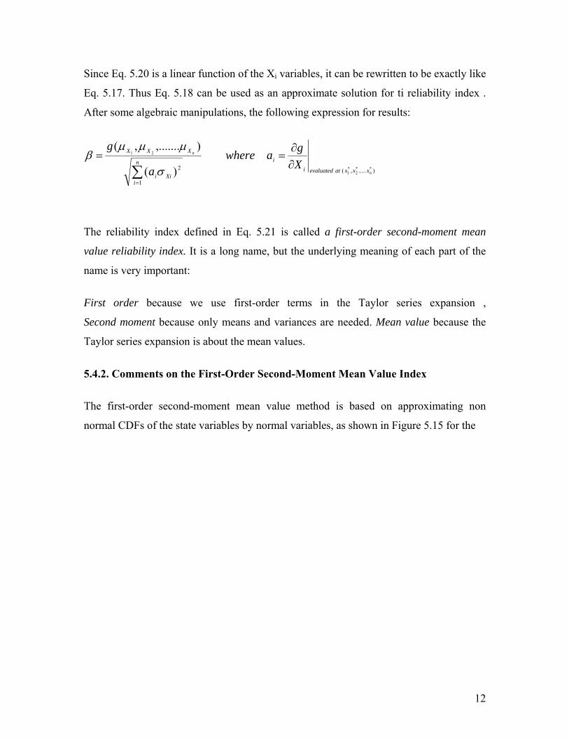
Since Eq. 5.20 is a linear function of the Xi variables, it can be rewritten to be exactly like

Eq. 5.17. Thus Eq. 5.18 can be used as an approximate solution for ti reliability index .

After some algebraic manipulations, the following expression for results:

).....,(

1

2 **2

*1

21

)(

),.......,(

n

n

xxxatevaluatediin

iXii

XXX

Xgawhere

a

g∂∂

==∑

=

σ

μμμβ

The reliability index defined in Eq. 5.21 is called a first-order second-moment mean

value reliability index. It is a long name, but the underlying meaning of each part of the

name is very important:

First order because we use first-order terms in the Taylor series expansion ,

Second moment because only means and variances are needed. Mean value because the

Taylor series expansion is about the mean values.

5.4.2. Comments on the First-Order Second-Moment Mean Value Index

The first-order second-moment mean value method is based on approximating non

normal CDFs of the state variables by normal variables, as shown in Figure 5.15 for the

12

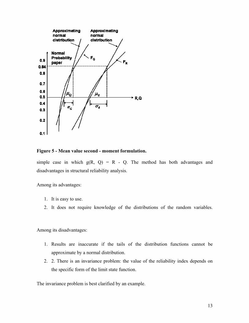
Figure 5 - Mean value second - moment formulation.

simple case in which g(R, Q) = R - Q. The method has both advantages and

disadvantages in structural reliability analysis.

Among its advantages:

1. It is easy to use.

2. It does not require knowledge of the distributions of the random variables.

Among its disadvantages:

1. Results are inaccurate if the tails of the distribution functions cannot be

approximate by a normal distribution.

2. 2. There is an invariance problem: the value of the reliability index depends on

the specific form of the limit state function.

The invariance problem is best clarified by an example.

13

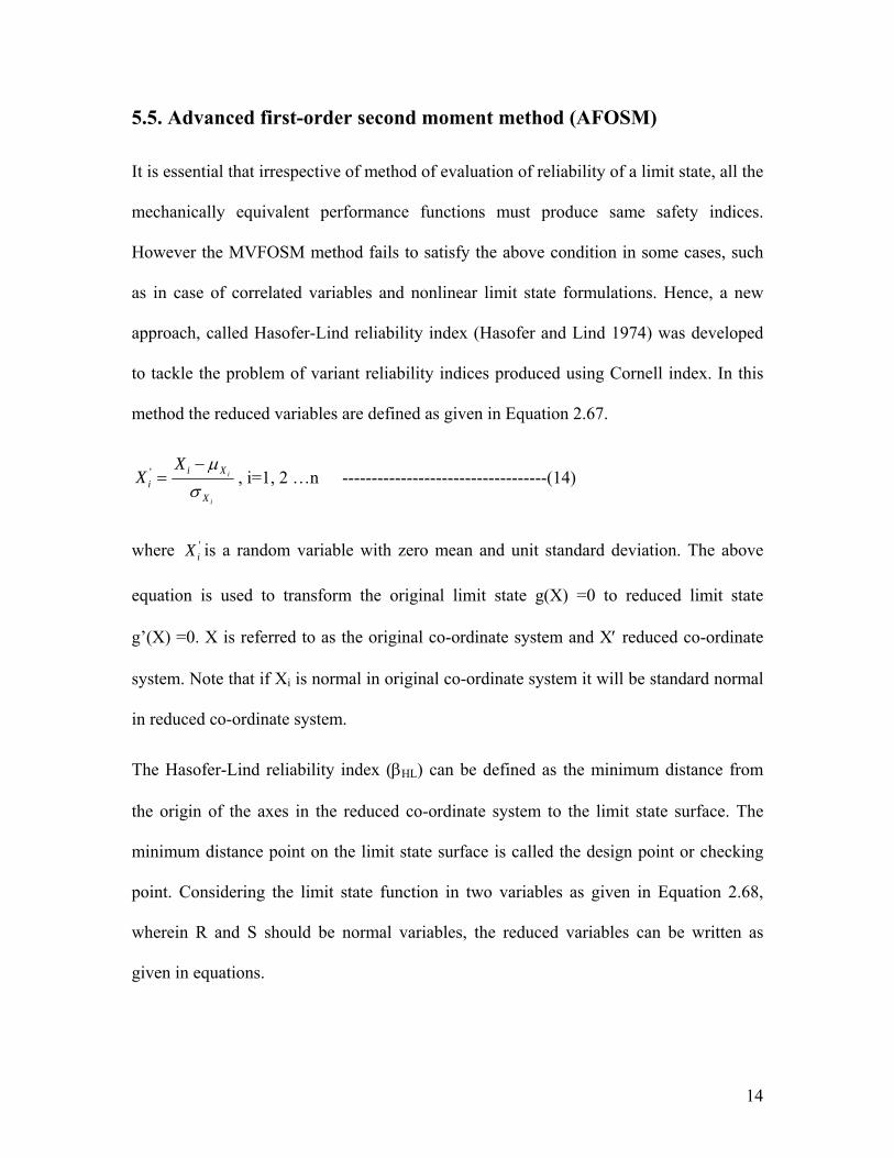
5.5. Advanced first-order second moment method (AFOSM)

It is essential that irrespective of method of evaluation of reliability of a limit state, all the

mechanically equivalent performance functions must produce same safety indices.

However the MVFOSM method fails to satisfy the above condition in some cases, such

as in case of correlated variables and nonlinear limit state formulations. Hence, a new

approach, called Hasofer-Lind reliability index (Hasofer and Lind 1974) was developed

to tackle the problem of variant reliability indices produced using Cornell index. In this

method the reduced variables are defined as given in Equation 2.67.

i

i

X

Xii

XX

σμ−

=' , i=1, 2 …n -----------------------------------(14)

where is a random variable with zero mean and unit standard deviation. The above

equation is used to transform the original limit state g(X) =0 to reduced limit state

g’(X) =0. X is referred to as the original co-ordinate system and X′ reduced co-ordinate

system. Note that if X

'iX

i is normal in original co-ordinate system it will be standard normal

in reduced co-ordinate system.

The Hasofer-Lind reliability index (βHL) can be defined as the minimum distance from

the origin of the axes in the reduced co-ordinate system to the limit state surface. The

minimum distance point on the limit state surface is called the design point or checking

point. Considering the limit state function in two variables as given in Equation 2.68,

wherein R and S should be normal variables, the reduced variables can be written as

given in equations.

14

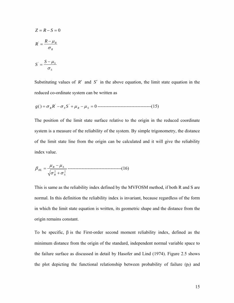
0=−= SRZ

R

RRRσ

μ−='

S

SSSσ

μ−='

Substituting values of R′ and S ′ in the above equation, the limit state equation in the

reduced co-ordinate system can be written as

0)( '' =−+−= SRSR SRg μμσσ -----------------------------------(15)

The position of the limit state surface relative to the origin in the reduced coordinate

system is a measure of the reliability of the system. By simple trigonometry, the distance

of the limit state line from the origin can be calculated and it will give the reliability

index value.

22SR

SRHL

σσ

μμβ

+

−= -----------------------------------(16)

This is same as the reliability index defined by the MVFOSM method, if both R and S are

normal. In this definition the reliability index is invariant, because regardless of the form

in which the limit state equation is written, its geometric shape and the distance from the

origin remains constant.

To be specific, β is the First-order second moment reliability index, defined as the

minimum distance from the origin of the standard, independent normal variable space to

the failure surface as discussed in detail by Hasofer and Lind (1974). Figure 2.5 shows

the plot depicting the functional relationship between probability of failure (pf) and

15

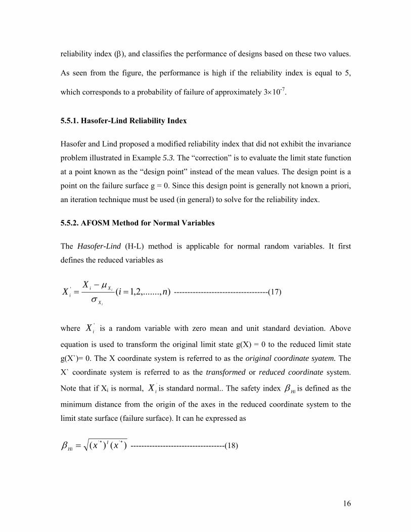
reliability index (β), and classifies the performance of designs based on these two values.

As seen from the figure, the performance is high if the reliability index is equal to 5,

which corresponds to a probability of failure of approximately 3×10-7.

5.5.1. Hasofer-Lind Reliability Index

Hasofer and Lind proposed a modified reliability index that did not exhibit the invariance

problem illustrated in Example 5.3. The “correction” is to evaluate the limit state function

at a point known as the “design point” instead of the mean values. The design point is a

point on the failure surface g = 0. Since this design point is generally not known a priori,

an iteration technique must be used (in general) to solve for the reliability index.

5.5.2. AFOSM Method for Normal Variables

The Hasofer-Lind (H-L) method is applicable for normal random variables. It first

defines the reduced variables as

),.......,2,1(' niX

Xi

i

X

Xii =

−=

σμ

-----------------------------------(17)

where is a random variable with zero mean and unit standard deviation. Above

equation is used to transform the original limit state g(X) = 0 to the reduced limit state

g(X`)= 0. The X coordinate system is referred to as the original coordinate syatem. The

X` coordinate system is referred to as the transformed or reduced coordinate system.

Note that if X

'iX

i is normal, ` is standard normal.. The safety index iX Hiβ is defined as the

minimum distance from the origin of the axes in the reduced coordinate system to the

limit state surface (failure surface). It can he expressed as

)()( `*`* xx IHi =β -----------------------------------(18)

16

The minimum distance point on the limit state surface is called the design point or

checking point. It is denoted by vector x* in the original coordinate system and by vector

x`* in the reduced coordinate system. These vectors represent the values of all the

random variables, that is, X1, X2. ..., Xn, at the design point corresponding to the

coordinate system being used.

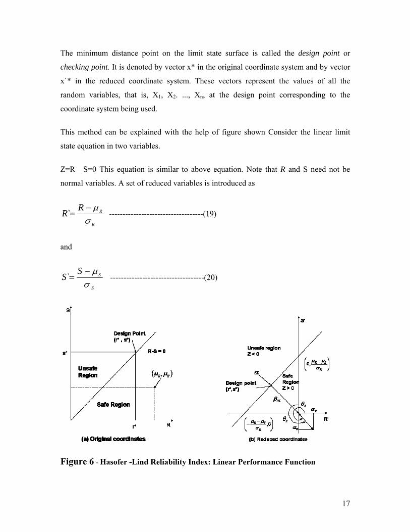
This method can be explained with the help of figure shown Consider the linear limit

state equation in two variables.

Z=R—S=0 This equation is similar to above equation. Note that R and S need not be

normal variables. A set of reduced variables is introduced as

R

RRRσ

μ−=̀ -----------------------------------(19)

and

S

SSSσ

μ−=̀ -----------------------------------(20)

Figure 6 - Hasofer -Lind Reliability Index: Linear Performance Function

17

If we substitute these into above equation the limit state equation in the reduced

coordinate system becomes

( ) 0'' =−+−= SRSR SRg μμσσ -----------------------------------(21)

The transformation of the limit state equation from the original to the reduced coordinate

system is shown in above figure. The safe and failure regions are also shown. From the

figure, it is apparent that if the failure line (limit state line) is closer to the origin in the

reduced coordinate system the failure region is larger and if it is farther away from the

origin, the failure region is smaller. Thus, the position of the limit state surface relative to

the origin in the reduced coordinate system is a measure of the reliability of the system.

The coordinates of the intercepts of a on the R` and S` axes can be shown

to be

bove equation

( )[ ] ( )[ ]SSRRSR and σμμσμμ /,00,/ −−− , respectively .Using simple

trigonometry, we can calculate the distance of the limit state line from the origin as

22SR

SRHL

σσ

μμβ

+

−= -----------------------------------(22)

This distance is referred to as the reliability index or safety index. It is the same as the

reliability index defined by the MVFOSM method in above equation if both R and S are

normal variables. However, it is obtained in a completely different way based on

geometry. It indicates that if the limit state is linear and if the random variables R and S

arc normal, both methods will give an identical reliability or safety index.

…..xn) in

ates the safe state and g(X’) < 0 denotes the failure state, Again, the Hasofer-

ned coordinated system and 21 ........,, nXXXXX

In general, for many random variables represented by the vector X = (x1,x2,…

the origin

Lind reliability index is defi ````` = 3 in

the reduced coordinate system the limit state g(X`) = 0 is a nonlinear function as shown

in the reduced coordinates for two variables in figure .At this stage, 'iX s are assumed to

be uncorrelated. Here g(X`) > 0 denoted as the minimum distance from the origin to the

design point on the limit state in the reduced coordinates and can be expressed by above

equation , where x` - represents the coordinates of the design point or the point of

minimum distance from the origin to the limit state. In this definition the reliability index

is invariant, because regardless of the form in which the limit state equation is written, its

`

18

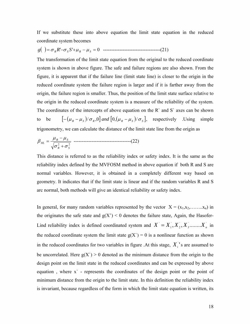
geometric shape and the distance from the origin remain constant. For the limit state

surface where ,

the failure region is away from the origin

ilure point. The Hasofer-L

Figure 7 - Hasofer - Lind Reliability Index: Nonlinear Performance Function

it is easy to see from figure that x` is the most probable fa ind

reliability index can be used to calculate a first-order approximation of the failure

probability as This is the integral of the standard norm

the larger is the failure probability. Thus the minimum distance point on the limit state

surface is also the most probable failure point. The point of minimum distance from the

origin to the limit state surface, x`*, represents the worst combination of the stochastic

variables and is appropriately named the design point or the most probable point (MPP)

of failure.

For nonlinear limit states, the computation of the minimum distance becomes an

optimization problem:

al density function

along the ray joining the origin and x`* it is obvious that the nearer x`* is to the origin,

'' xxDMinimized l=

( ) ( ) 0'int == xgxgconstrathetoSubjected

where x` represents the coordinates of the checking point on the limit state equation in

the reduced coordinates to be estimated. Using the method of Lagrange multipliers, we

can obtain the minimum distance as

19

∑

∑

=

=

⎟⎟⎠

⎞⎜⎜⎝

⎛∂∂

⎟⎟⎠

⎞⎜⎜⎝

⎛∂∂

−=n

i i

i

n

ii

HL

Xg

Xgx

1

*2

'

*

'1

'*

β -----------------------------------(23)

Where is the ith partial derivative evaluated at the design point with

coordinates

( )*'/ iXg ∂∂

( )'*'*2

'*1 ....., nxxx . The asterisk after the derivative indicates that it is evaluated at

( )'*'*'* ....., xxx . The design point in the reduced coordinates is given by: 21 n

( )nix HLii ,.......2,1'* =−= βα

Where

∑=

*

An algorithm was form lated by Rackwitz (1976) to compute

⎟⎟⎠

⎞⎜⎜⎝

⎛∂∂

⎟⎟⎠

⎞⎜⎜⎝

⎛∂∂

=n

i i

ii

Xg

Xg

1

*2

'

'

α - ----------------------------------(24)

are the direction cosines along the coordinate axes ' in the space of the original iX

coordinates and using equation, we find the design point to be

HLXiXi iix βσαμ −=*

HLβu and as follows:

• Step 1. Define the appropriate limit state equation.

e initial values of the design point . Typically, the

'*ix

nixi ..,.........2,1,'* =• Step 2. Assum

initial design point may be assumed to be at the mean values of the random variables.

Obtain the reduced variates ( )ii XXii xx σμ−='* .

• Step 3. Evaluate ( ) '*iii xat

• Step 4. Obtain the new design point in terms of

'* andXg α∂∂

'*ix HLβ as in equation.

• Step 5. Substitute the new in the limit state equation g(x`*) = 0 and solve for '*ix HLβ .

20

HLβ• Step 6. Using the value obtained in Steps 5. Re-evaluate

• Step 7. Repeat Steps

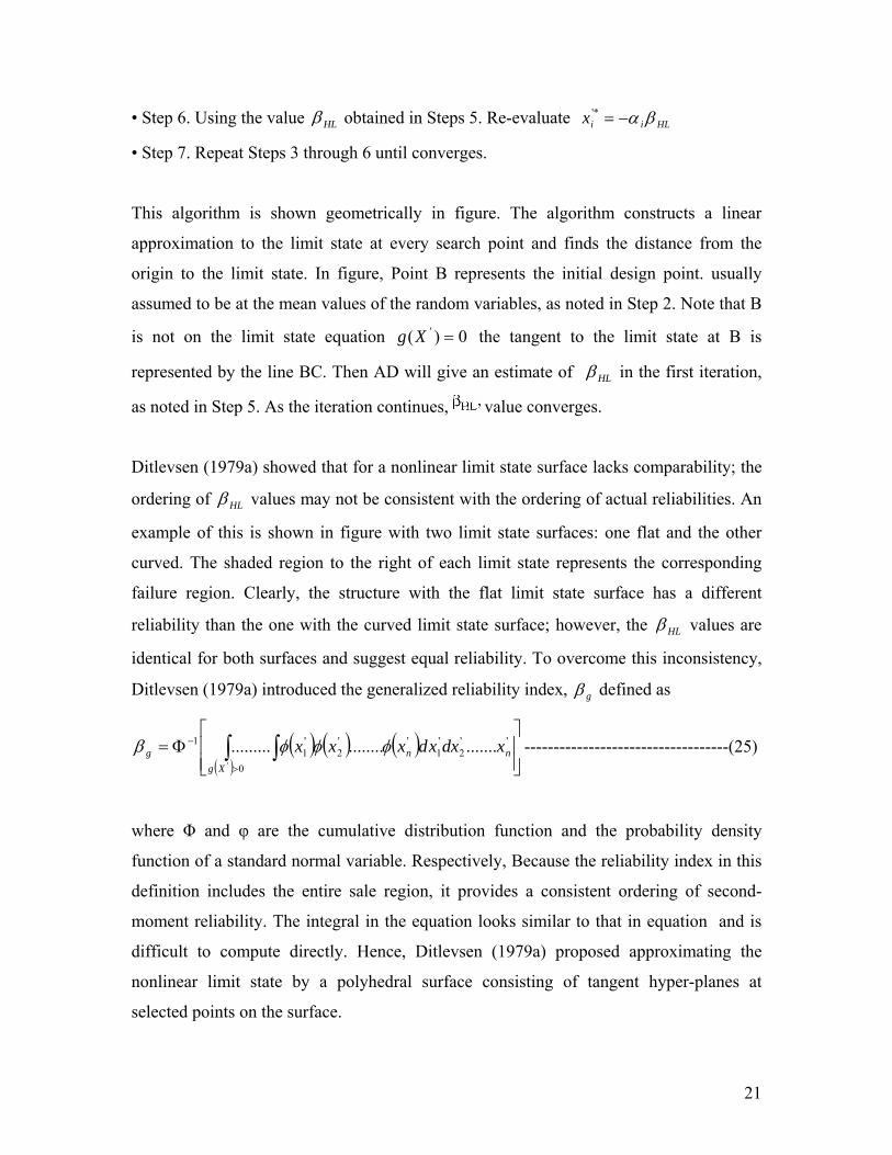
This algorithm is shown geometrically in figure. The algorithm constructs a linear

pproximation to the limit state at every search point and finds the distance from the

o the limit

assumed to be at the mean values of the random variables, as noted in Step 2. Note that B

it state equation

represented b

HLiix βα−='*

3 through 6 until converges.

a

origin t state. In figure, Point B represents the initial design point. usually

is not on the lim 0)( ' =Xg the tangent to the limit state at B is

y the line BC. Then AD will give an estimate of HLβ in the first iteration,

s noted in Step 5. As the iteration continues, a value converges.

Ditlevsen (1979a) showed that for a nonlinear limit state surface lacks comparability; the

ordering of

HLβ va rdering of actual reliabilities. An

example of this is shown in figure with two limit state surfaces: one flat and the other

curved. The shaded region to the right of each limit state represents the corresponding

ilure region. Clearly, the structure with the flat limit state surface has a different

e

lues may not be consistent with the o

fa

reliability than the one with the curved limit state surfac ; however, the HLβ values are

identical for both surfaces and suggest equal reliability. To overcom sistency,

Ditlevsen (1979a) introduced the generalized reliability index,

e this incon

gβ defined as

⎦2121 nng )

al variable. Respec se the reliability index in this

definition includes the entire sale region, it provides a consistent ordering of second-

. The integral in the eq tion looks similar to that in equation and is

979 roximating the

nes t

( ) ( ) ( ) ⎥⎤

⎢⎡

Φ= ∫ ∫− ''''''1 ........................ xdxxdxxx φφφβ -----------------------------------(25( )⎢⎣ >0'Xg ⎥

where Φ and φ are the cumulative distribution function and the probability density

function of a standard norm tively, Becau

moment reliability ua

difficult to compute directly. Hence, Ditlevsen (1 a) proposed app

nonlinear limit state by a polyhedral surface consisting of tangent hyper-pla a

selected points on the surface.

21

igure 8 - Algorithm for finding βHL F Note: A number in parentheses indicates iteration numbers

Consider a limit state function g(X1, X2, . . . , Xn) where the random variables Xi are all

uncorrelated. (If the variables are correlated, then a transformation can be used to obtain

uncorrelated variables. See Example 5.15.) The limit state function is rewritten in terms

of the standard form of the variables (reduced variables) using

i

iXiXZ

Xi σ

μ−=

As before, the Hasofer-Lind reliablity index is defined as the shortest distance from the

rigin of the reduced variable space to the limit state function g = 0. o

Thus far nothing has changed from the previous presentation of the reliability index. In

fact, if the limit state function is linear, then the reliability index is still calculated as in

Eq 5.18

∑

∑

=

=

+=

n

iXi

n

iXi

i

i

a

aa

1

2

10

)( σ

μβ

-------------------------------- (26)

22

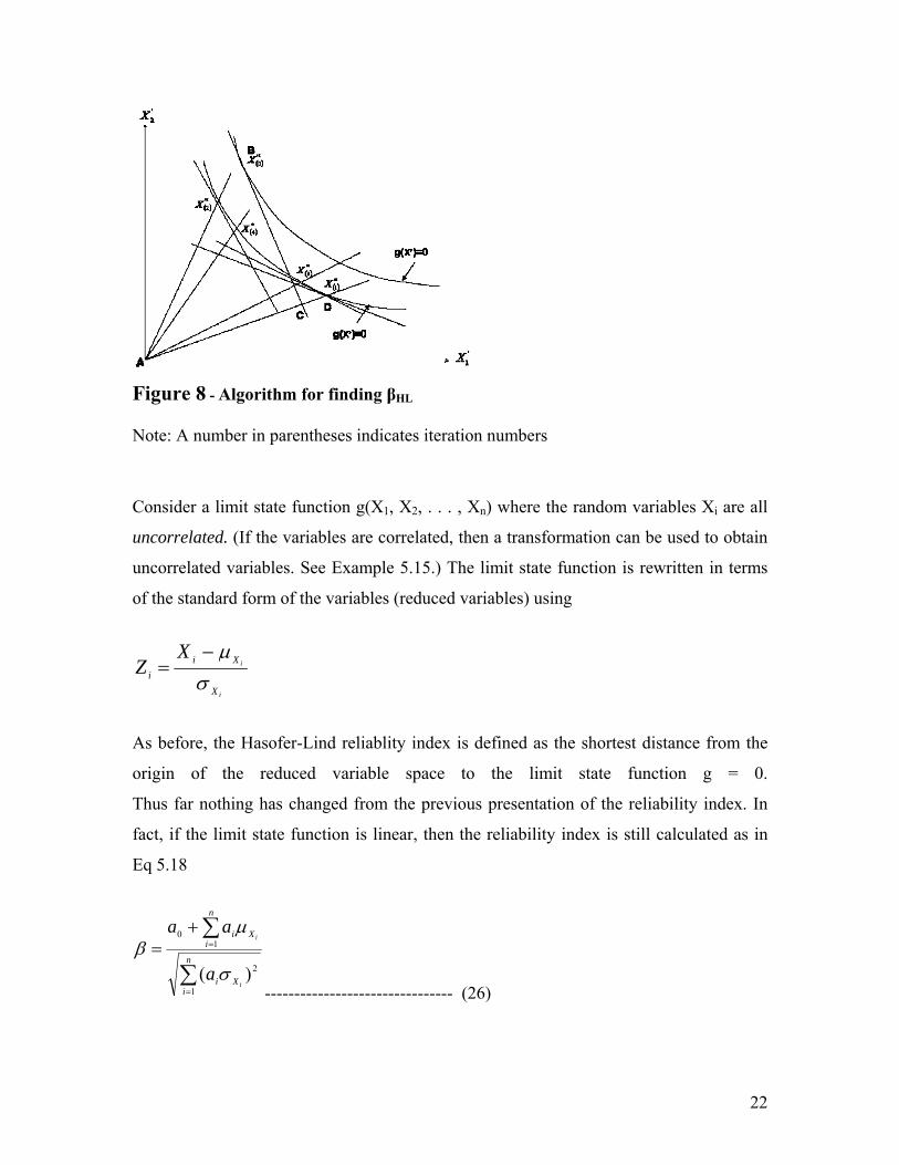
If the limit state function is nonlinear , however, iteration is required to find the design

point in reduced variable space such that still corresponds to the

Shortest distance. This concept is illustrated in Figures 5.17 through 5.19 for the case of

two random variables.

}......,{ **2

*1 nZZZ

Figure 9 - Hasofer - Lind reliability index

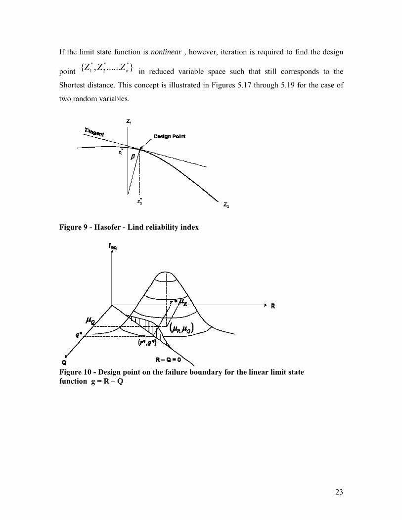
Figure 10 - Design point on the failure boundary for the linear limit state function g = R – Q

23

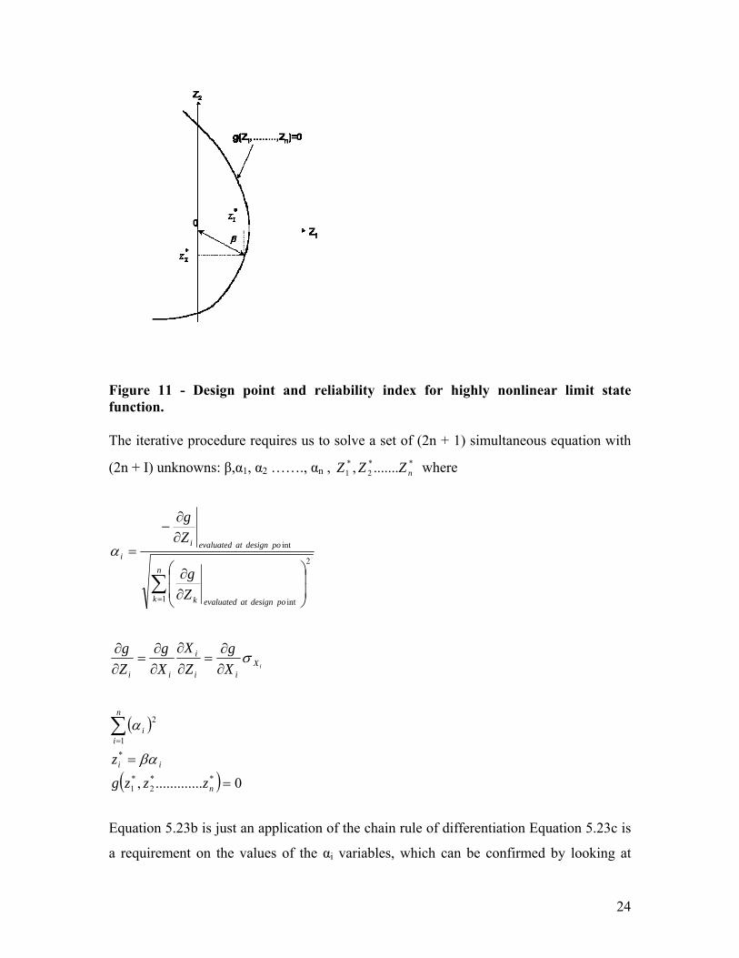
Figure 11 - Design point and reliability index for highly nonlinear limit state function.

he iterative procedure requires us to solve a set of (2n + 1) simultaneous equation with

(2n + I) unknowns: β,α1, α2 ……., αn , where

T**

2*1 ......., nZZZ

∑= ⎟

⎟

⎠

⎞

⎜⎜

⎝

⎛

∂∂

∂∂

−

=n

k podesignatevaluatedk

podesignatevaluatedii

Zg

Zg

1

2

int

intα

iXii

i

ii Xg

ZX

Xg

Zg σ

∂∂

=∂∂

∂∂

=∂∂

( )

( ) 0............., **2

*1

*1

2

=

=

∑=

n

ii

ii

zzzg

z βα

α

Equation 5.23b is just an application of the chain rule of differentiation Equation 5.23c is

a requirement on the values of the αi variables, which can be confirmed by looking at

n

24

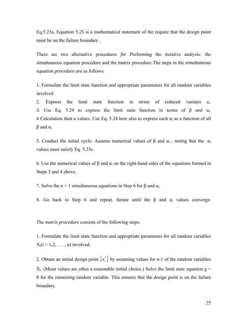
Eq.5.23a. Equation 5.25 is a mathematical statement of the require that the design point

must be on the failure boundary .

There are two alternative procedures for Performing the iterative analysis: the

simultaneous equation procedure and the matrix procedure The steps in the simultaneous

equation procedure are as follows:

1. Formulate the limit state function and appropriate parameters for all random variables

involved

2. Express the limit state function in terms of reduced variates zi.

3. Use Eq. 5.24 to express the limit state function in terms of β and αi.

4 Calculation then a values. Use Eq. 5.24 here also to express each αi as a function of all

5. Conduct the initial cycle: Assume numerical values of β and αi , noting that the αi

6. Use the numerical values of β and αi on the right-hand sides of the equations formed in

Steps 3 and 4 above.

7. Solve the n + 1 simultaneous equations in Step 6 for β and αi.

8. Go back to Step 6 and repeat. Iterate until the β and αi values converge.

The matrix procedure consists of the following steps:

1. Formulate the limit state function and appropriate parameters for all random variables

Xi(i = 1,2, . . . , n) involved.

2. Obtain an initial design point

β and αi.

values must satisfy Eq. 5.23c.

{ }*ix by assuming values for n-1 of the random variables

Xi. (Mean values are often a reasonable initial choice.) Solve the limit state equation g =

0 for the remaining random variable. This ensures that the design point is on the failure

boundary.

25

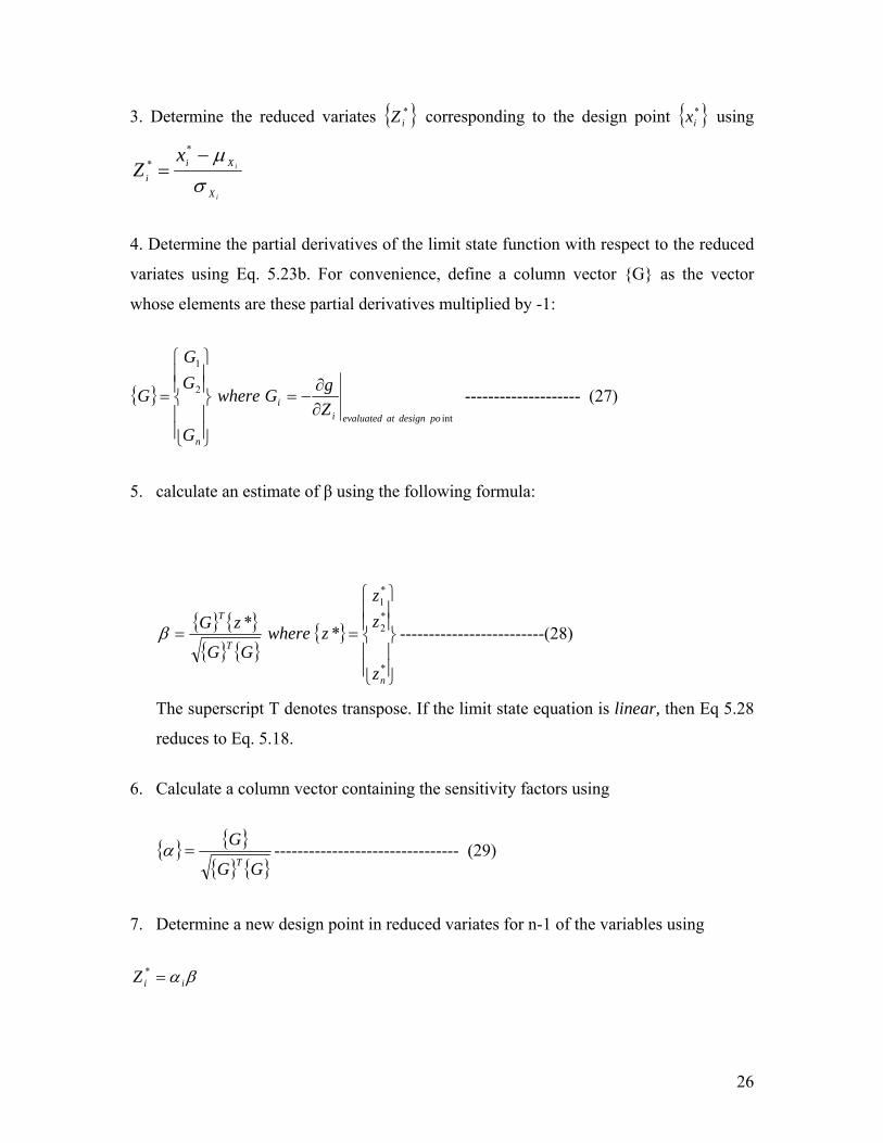
3. Determine the reduced variates { }*iZ corresponding to the design point { }*

ix using

iXσ

4. Determine the partial derivatives o

iXiiZ =*

the limit state function with respec duced

variates using Eq. 5.23b. For convenience, define a column vector {G} as the vector

x μ−*

f t to the re

whose elements are these partial derivatives multiplied by -1:

{ }int

2

1

podesignatevaluatedii

n

ZgGwhere

G

GG

G∂∂

−=

⎪⎪

⎪⎪⎬

⎫

⎪⎪⎩

⎪⎪⎨

⎧

= -------------------- (27)

⎭

5. calculate an estimate of β using the following formula:

{ } { }{ } { }

{ }

⎪⎪⎭⎪

⎪⎩

*zGG

⎪⎪⎬

⎪⎪⎨==

*2

1

*

n

T

zzwhereβ -------------------------(28)

reduces to Eq. 5.18.

factors using

⎫⎧ *

*T

zzG

The superscript T denotes transpose. If the limit state equation is linear, then Eq 5.28

6. Calculate a column vector containing the sensitivity

{ } { }{ } { }GG

GT

=α -------------------------------- (29)

7. Determine a new design point in reduced variates for n-1 of the variables using

βα iiZ =*

26

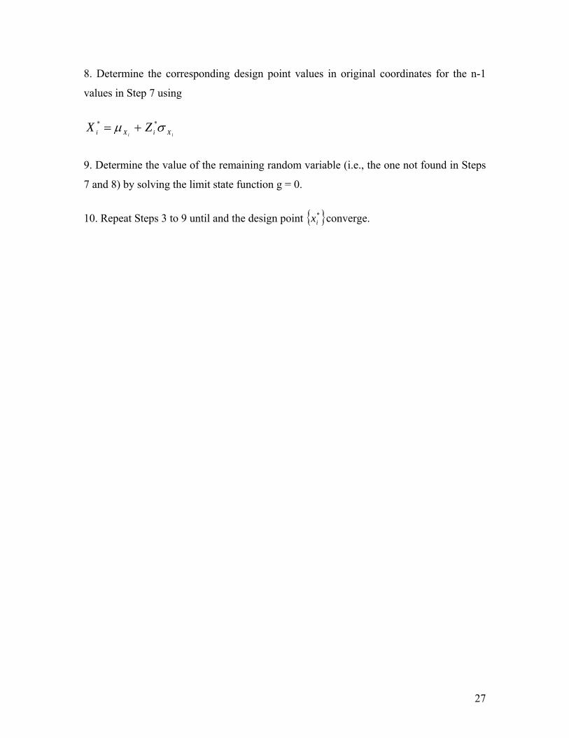
8. Determine the corresponding design point values in original coordinates for the n-1

values in Step 7 using

ii XiXi ZX σμ ** +=

9. Determine the value of the remaining random variable (i.e., the one not found in Steps

7 and 8) by solving the limit state function g = 0.

10. Repeat Steps 3 to 9 until and the design point { }*ix converge.

27