5-1

5. FLOW OF WATER THROUGH SOIL

5.1 FLOW OF WATER IN A PIPE

The flow of water through a rough open pipe may be expressed by means of the Darcy-

Weisbach resistance equation

∆h = f L

D

v2

2g (5.1)

in which _h is the head loss over a length L of pipe of diameter D. The average velocity of flow is

v. f is a measure of pipe resistance.

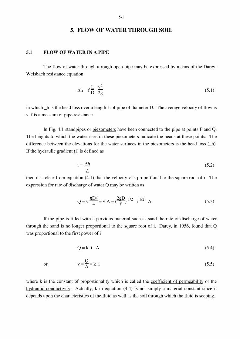
In Fig. 4.1 standpipes or piezometers have been connected to the pipe at points P and Q.

The heights to which the water rises in these piezometers indicate the heads at these points. The

difference between the elevations for the water surfaces in the piezometers is the head loss (_h).

If the hydraulic gradient (i) is defined as

i =

L

h∆ (5.2)

then it is clear from equation (4.1) that the velocity v is proportional to the square root of i. The

expression for rate of discharge of water Q may be written as

Q = v πD2

4 = v A = (

2gD

f)

1/2 i

1/2 A (5.3)

If the pipe is filled with a pervious material such as sand the rate of discharge of water

through the sand is no longer proportional to the square root of i. Darcy, in 1956, found that Q

was proportional to the first power of i

Q = k i A (5.4)

or v = Q

A = k i (5.5)

where k is the constant of proportionality which is called the coefficient of permeability or the

hydraulic conductivity. Actually, k in equation (4.4) is not simply a material constant since it

depends upon the characteristics of the fluid as well as the soil through which the fluid is seeping.

5-2

Equation (4.4) or (4.5) expresses what has come to be known as Darcy’s Law. Several

studies have found that the relationship between v and i is non linear but this has been largely

discounted by Mitchell (1976) who concluded that if all other factors are held constant, Darcy’s

Law is valid. Because of the small value of v that applies to water seeping through soil, the flow

is considered to be laminar. For coarse sands and gravels the flow may not be laminar so the

validity of Darcy’s Law in these cases may be in doubt.

5.2 THE COEFFICIENT OF PERMEABILITY

Typical values of k for various types of soil are shown in Table 5.1. This table illustrates

the enormous range of values of permeability for soils.

TABLE 5.1

TYPICAL VALUES OF PERMEABILITY

Gravel greater than 10-2 m/sec

Sand 10-6 m/sec to 10-2 m/sec

Silt 10-9 m/sec to 10-5 m/sec

Clay 10-11 m/sec to 10-8 m/sec

Several empirical equations have been proposed for the evaluation of the coefficient of

permeability. One of the earliest is that proposed by Hazen for uniform sands

k (cm/sec) = C1 D 2

10 (5.6)

where D10 = effective size in mm

C1 = constant, varying from 1.0 to 1.5

It was mentioned above that the coefficient of permeability (k) is not strictly a material

constant. The viscosity and density of the permeant have been found to influence the value of k.

The two characteristics may be eliminated by using “absolute permeability” (K) having

dimensions of (length)2 and defined as

K = k (µ

ρwg) (5.7)

where µ is the viscosity of the permeant.

5-3

Fig. 5.1 Flow Through a Pipe

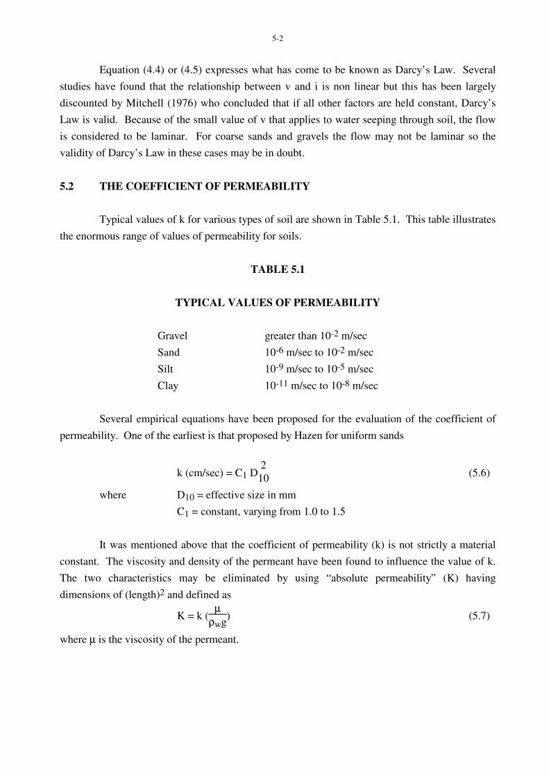
Fig. 5.2 Flow Rates versus Porosity

(after Olsen, 1962)

5-4

In carrying out permeability tests the viscosity is standardized by carrying out the tests at

20˚C or by making a correction for tests carried out at other temperatures.

k20 = kt (µt/µ20) (5.8)

where k20 = coefficient of permeability at 20˚C

kt = coefficient of permeability at temperature t

µ20 = viscosity at 20˚C

µt = viscosity at temperature t

An equation that has been proposed for absolute permeability (K) of sandy soils is the

Kozeny-Carman equation.

K = 1

ko T2 S2

0

(e3

1 + e) (5.9)

where ko is a pore shape factor (~~ 2.5)

T is the tortuosity factor (~~21/2)

So is the specific surface area per unit volume of particles

e is the void ratio

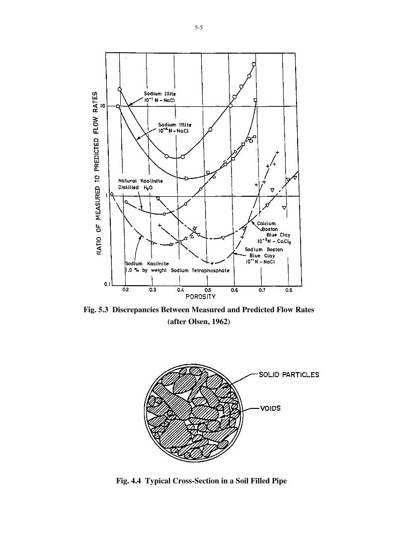
The Kozeny-Carman equation has been found to work well with sands but is inadequate

with clays. This inadequacy with clays is illustrated in Figures 4.2 and 4.3. Olsen (1962) has

shown that the major reason for these discrepancies with clay soils is the existence of unequal

pore sizes.

The preceding comments indicate that several factors may influence the permeability of a

soil, and these must be taken into account particularly when laboratory tests are used to assess the

permeability of a soil stratum.

5.3 WHAT IS v?

The v in equation (5.5) is known as the superficial or discharge velocity for the very good

reason that it is not the actual velocity of flow of the water through the soil.

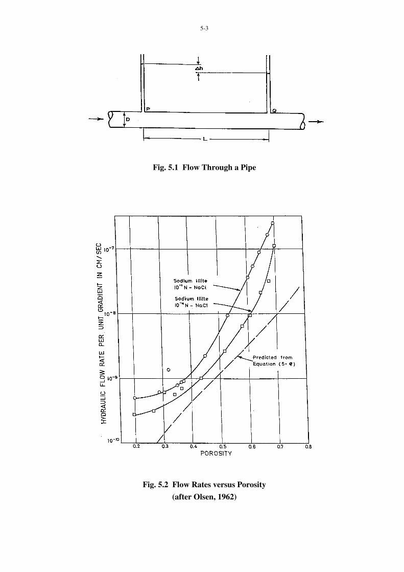
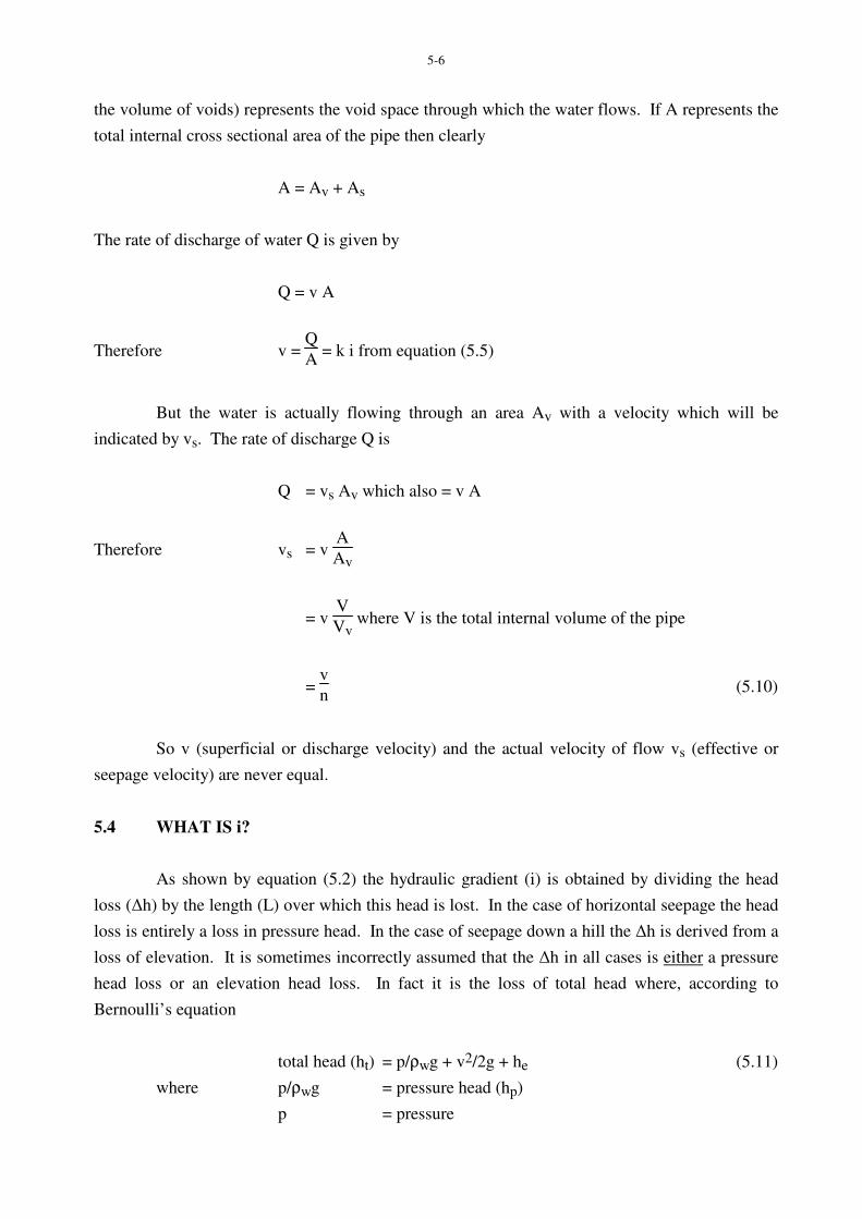
Consider a typical cross section through the soil in the pipe as illustrated in Fig. 5.4. The

hatched portion represents the soil mineral particles of soil with an average cross sectional are

equal to As. The remaining cross sectional area in the pipe Av (= Vv

L where L is the length of pipe

and Vv is

5-5

Fig. 5.3 Discrepancies Between Measured and Predicted Flow Rates

(after Olsen, 1962)

Fig. 4.4 Typical Cross-Section in a Soil Filled Pipe

5-6

the volume of voids) represents the void space through which the water flows. If A represents the

total internal cross sectional area of the pipe then clearly

A = Av + As

The rate of discharge of water Q is given by

Q = v A

Therefore v = Q

A = k i from equation (5.5)

But the water is actually flowing through an area Av with a velocity which will be

indicated by vs. The rate of discharge Q is

Q = vs Av which also = v A

Therefore vs = v A

Av

= v V

Vv where V is the total internal volume of the pipe

= v

n (5.10)

So v (superficial or discharge velocity) and the actual velocity of flow vs (effective or

seepage velocity) are never equal.

5.4 WHAT IS i?

As shown by equation (5.2) the hydraulic gradient (i) is obtained by dividing the head

loss (∆h) by the length (L) over which this head is lost. In the case of horizontal seepage the head

loss is entirely a loss in pressure head. In the case of seepage down a hill the ∆h is derived from a

loss of elevation. It is sometimes incorrectly assumed that the ∆h in all cases is either a pressure

head loss or an elevation head loss. In fact it is the loss of total head where, according to

Bernoulli’s equation

total head (ht) = p/ρwg + v2/2g + he (5.11)

where p/ρwg = pressure head (hp)

p = pressure

5-7

v2/2g = velocity head (hv)

he = elevation head

In seepage problems the velocity of flow is very small and the velocity head is negligible in

comparison with the pressure and elevation heads. Therefore in seepage problems

ht = he + hp (5.12)

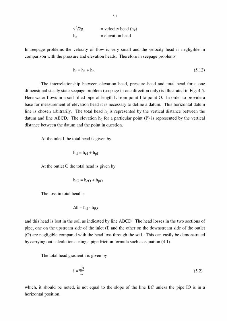
The interrelationship between elevation head, pressure head and total head for a one

dimensional steady state seepage problem (seepage in one direction only) is illustrated in Fig. 4.5.

Here water flows in a soil filled pipe of length L from point I to point O. In order to provide a

base for measurement of elevation head it is necessary to define a datum. This horizontal datum

line is chosen arbitrarily. The total head ht is represented by the vertical distance between the

datum and line ABCD. The elevation he for a particular point (P) is represented by the vertical

distance between the datum and the point in question.

At the inlet I the total head is given by

htI = heI + hpI

At the outlet O the total head is given by

htO = heO + hpO

The loss in total head is

∆h = htI - htO

and this head is lost in the soil as indicated by line ABCD. The head losses in the two sections of

pipe, one on the upstream side of the inlet (I) and the other on the downstream side of the outlet

(O) are negligible compared with the head loss through the soil. This can easily be demonstrated

by carrying out calculations using a pipe friction formula such as equation (4.1).

The total head gradient i is given by

i = _h

L (5.2)

which, it should be noted, is not equal to the slope of the line BC unless the pipe IO is in a

horizontal position.

5-8

Fig. 5.5 One Dimensional Seepage

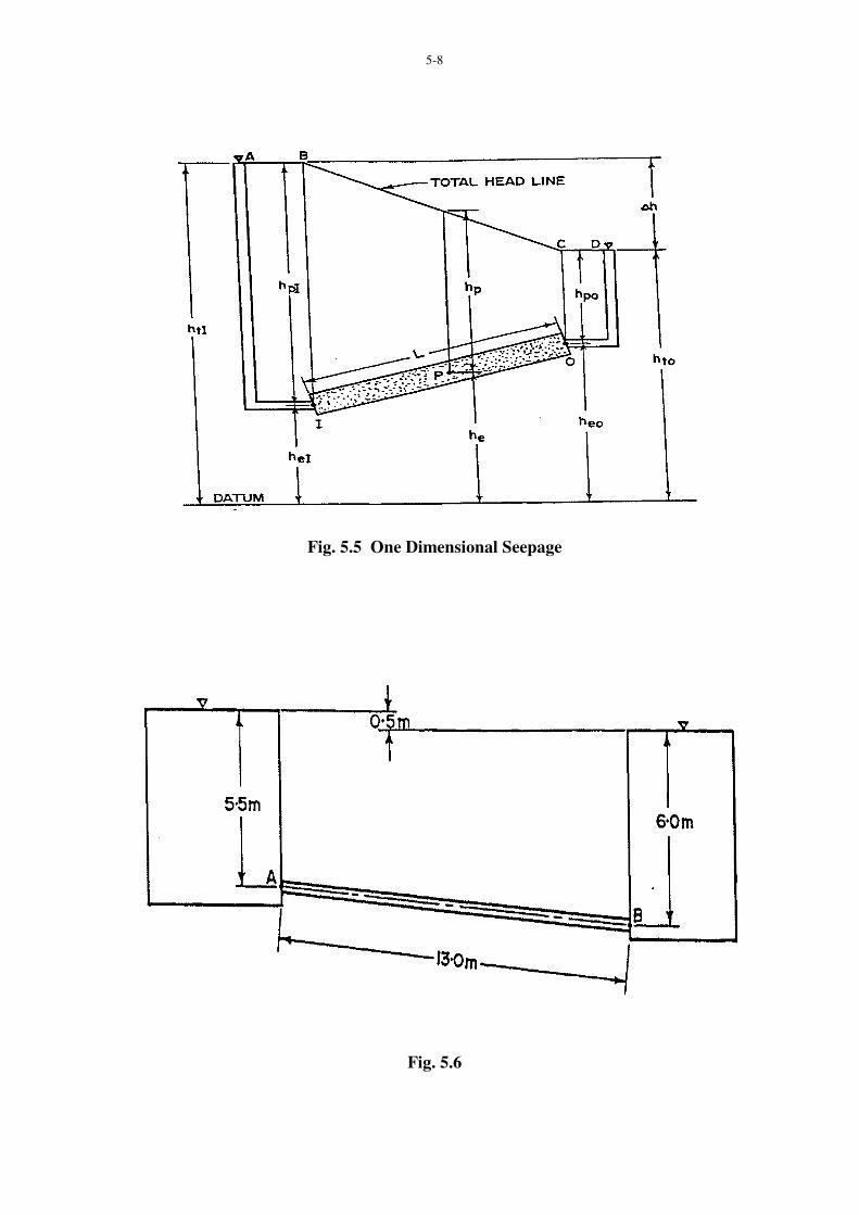
Fig. 5.6

5-9

5.5 PORE PRESSURE IN THE SOIL

The pressure head hp is a measure (in units of length) of the pore pressure of the water in

the soil. Again referring to Fig. 4.5 the pressure head at any point P may be found by measuring

the vertical distance (hp) between point P and the total head line ABCD. In other words if a

piezometric tube was inserted into the soil at point P and suspended upwards with the end of the

tube open to atmospheric pressure the water would rise in the tube a distance hp above point P.

The pore pressure (u) may be calculated from the pressure head (hp) by means of the

expression

u = ρwg hp (5.13)

where ρw = density of water

g = acceleration due to gravity

EXAMPLE

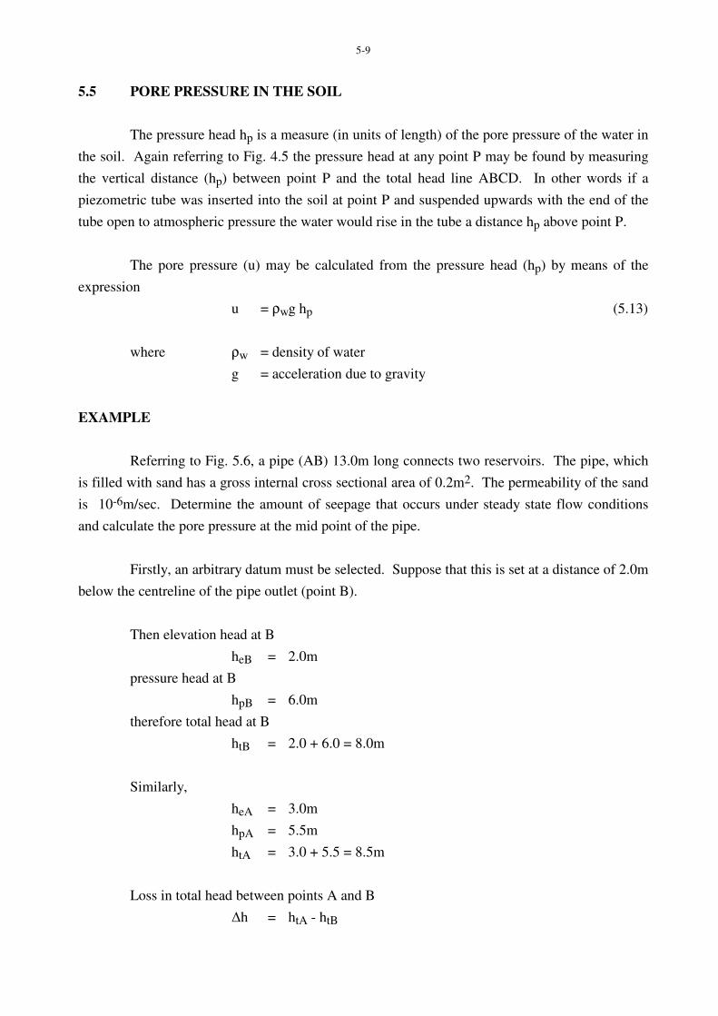
Referring to Fig. 5.6, a pipe (AB) 13.0m long connects two reservoirs. The pipe, which

is filled with sand has a gross internal cross sectional area of 0.2m2. The permeability of the sand

is 10-6m/sec. Determine the amount of seepage that occurs under steady state flow conditions

and calculate the pore pressure at the mid point of the pipe.

Firstly, an arbitrary datum must be selected. Suppose that this is set at a distance of 2.0m

below the centreline of the pipe outlet (point B).

Then elevation head at B

heB = 2.0m

pressure head at B

hpB = 6.0m

therefore total head at B

htB = 2.0 + 6.0 = 8.0m

Similarly,

heA = 3.0m

hpA = 5.5m

htA = 3.0 + 5.5 = 8.5m

Loss in total head between points A and B

∆h = htA - htB

5-10

= 8.5 - 8.0 = 0.5m

Note that this loss of total head is equal to the difference in elevations of the reservoir

water levels.

The gradient of total head

i = ∆h

L =

0.5

13.0

Using Darcy’s law, the rate of seepage flow

Q = k i A

= 10-6 x 0.5

13.0 x 0.2

= 0.77 x 10-8 m3/sec

As the total heads at points A and B are 8.5m and 8.0m respectively the total head at the mid point

of the pipe is 8.25m. The elevation head at the mid point of the pipe is 2.5m

∴ pressure head at mid point of pipe = 8.25 - 2.5 = 5.75m

pore pressure = ρwg hp

where ρw = 1000 kg/m3

g = 9.81 m/sec2

∴ pore pressure = 1000 x 9.81 x 5.75 N/m2

= 56.4 kN/m2

EXAMPLE

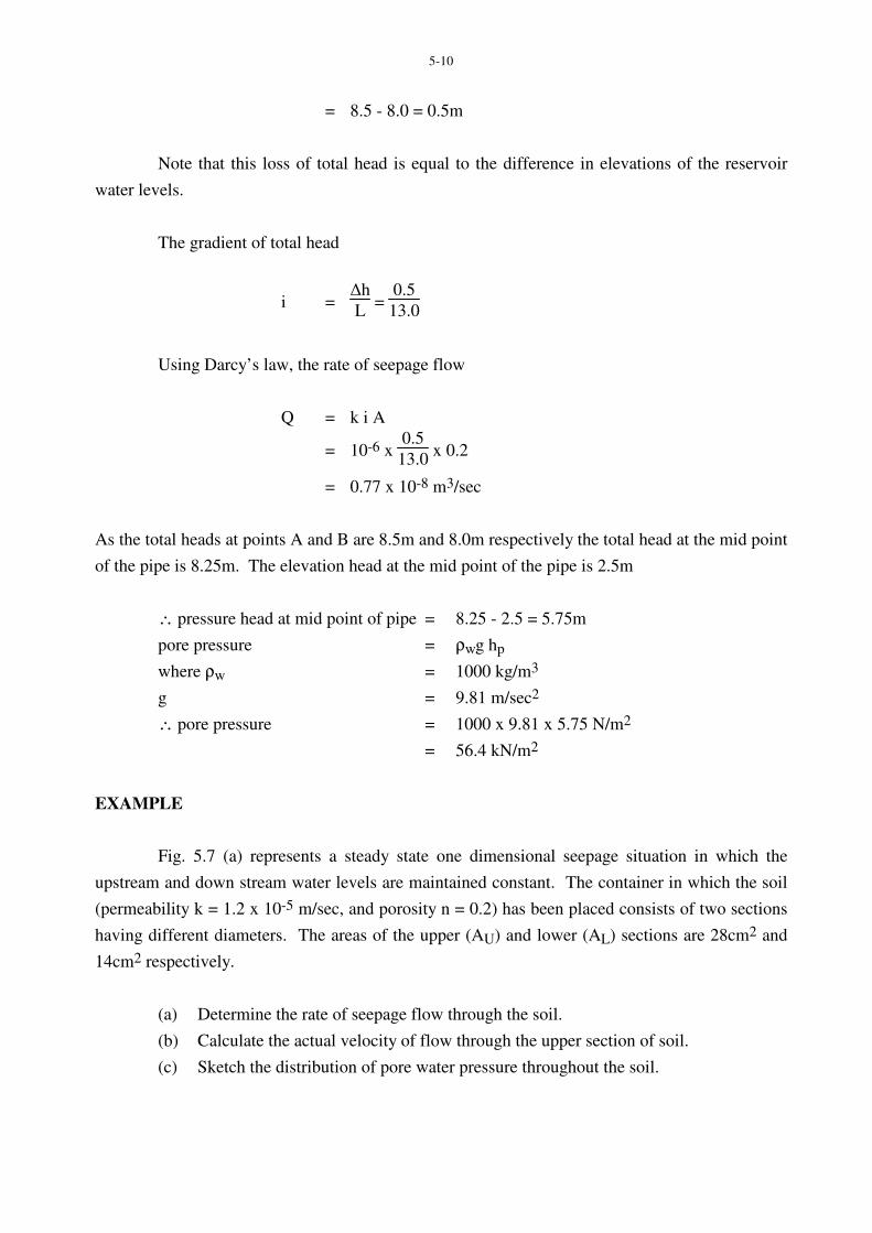
Fig. 5.7 (a) represents a steady state one dimensional seepage situation in which the

upstream and down stream water levels are maintained constant. The container in which the soil

(permeability k = 1.2 x 10-5 m/sec, and porosity n = 0.2) has been placed consists of two sections

having different diameters. The areas of the upper (AU) and lower (AL) sections are 28cm2 and

14cm2 respectively.

(a) Determine the rate of seepage flow through the soil.

(b) Calculate the actual velocity of flow through the upper section of soil.

(c) Sketch the distribution of pore water pressure throughout the soil.

5-11

Firstly it is necessary to establish an arbitrary datum from which the elevation head may

be measured. Let this datum be located a distance of 4cm below the lower boundary of the soil.

Fig. 5.7

Fig. 5.8 Falling Head Permeability Test

5-12

The elevation head line can now be drawn on a plot of head against distance above the datum as

illustrated in Fig. 5.7 (b).

The pressure head lines can now be drawn for the water on the upstream and downstream

sides of the soil. The pressure head for the upstream (lower) side of the soil is determined by the

distance below the upstream water level (left tube in Fig. 5.7 (a)). The distribution of pressure

head throughout the soil cannot be drawn at this stage.

The total head lines can now be found for the water on the upstream and downstream

sides of the soil by addition (represented horizontally in Fig. 5.7 (b)) of the pressure and elevation

head lines. As shown in Fig. 5.7 (b) the total heads on the upstream and downstream sides of the

soil are 64.0cm and 44.0cm respectively. This means that the loss in total head through the soil is

20.0cm (the same value as the elevation difference between the upstream and downstream water

levels).

hL - hU = 20.0

where hL and hU are the total head losses in the lower and upper sections of soil respectively.

Since the rate of flow through the upper and lower section must be equal

Q = k iL AL = k iU AU

or hL

LL . AL =

hU

LU . AU

hL

20.0 . 14.0 =

hU

16.0 . 28.0

∴ 2hL = 5hU

The two equations involving hL and hU can now be solved to yield

hL = 14.29cm and hU = 5.71cm

and the total head line can now be completed as shown in Fig.5.7 (b).

The rate of seepage flow can now be found

Q = k iL AL

5-13

= 1.2 x 10-5 x 102 x 14.29

20.0 x 14.0

= 1.2 x 10-2 cm3/sec

The actual velocity of flow or seepage velocity, vs in the upper section of soil is

vs = v

n (5.10)

= k iU

n

= 1.2 x 10-5 x 102 x 5.71

16.0 x

1

0.2

= 2.14 x 10-3 cm/sec

The pressure head line can be completed by subtracting the elevation head line from the

total head line. The pore water pressure at any point in the soil can now be found by multiplying

the pressure head at that point by ρwg.

5.6 EXPERIMENTAL DETERMINATION OF THE COEFFICIENT OF

PERMEABILITY

5.6.1 Constant Head Test

The value of k could be determined by means of equation (5.4) using the experimental

arrangement depicted in Fig. 5.5. The reservoir levels at A and D would be maintained constant

allowing steady state seepage through the soil sample to be established. The rate of discharge Q

would be observed over a convenient time interval. The permeability could then be determined

from

k = Q

A i =

QL

A∆h (5.14)

The experimental details are set out in books on soil testing such as Lambe (1951) and Bowles

(1970).

5-14

5.6.2 Falling Head Test

The falling head permeability test differs from the constant head permeability test in that

the upstream and/or downstream total heads do not remain constant throughout the test. Fig. 4.8

depicts a situation in which the upstream water level is allowed to fall in a standpipe having a

cross-sectional area a. The test commences with a head difference of hi between the upstream and

downstream water levels. At any time t after the commencement of the test the head difference

will be symbolized by h. At the end of the test time t1, the head difference is hf. Throughout the

test the downstream water level remains constant.

At time t, the rate of discharge is

Q = k i A

= k h

L A

and this must be equal to the rate of discharge through the standpipe

Q = - a dh

dt

∴ - a dh

dt = k

h

L A

- a ⌡⌠

hi

hf

dh

h =

k A

L ⌡⌠

o

t1 dt

∴ k = 2.3 aL

At1 log 10

hi

hf (5.15)

5.6.3 Field Determination of Permeability

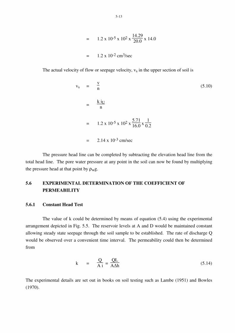
One of the many methods of determining k in the field is by means of a pump out test

(USBR, 1974). This test can be used in a situation which is represented in Fig. 5.9. A horizontal

stratum of previous soil containing a water table overlies an impervious stratum. A well is sunk

to the bottom of the pervious material and water is pumped from the well at a constant rate Q until

steady state conditions are reached. Observation wells at radial distances r1 and r2 permit

measurement of the heights h1 and h2 respectively.

5-15

Fig. 5.9 Field Pump Out Test

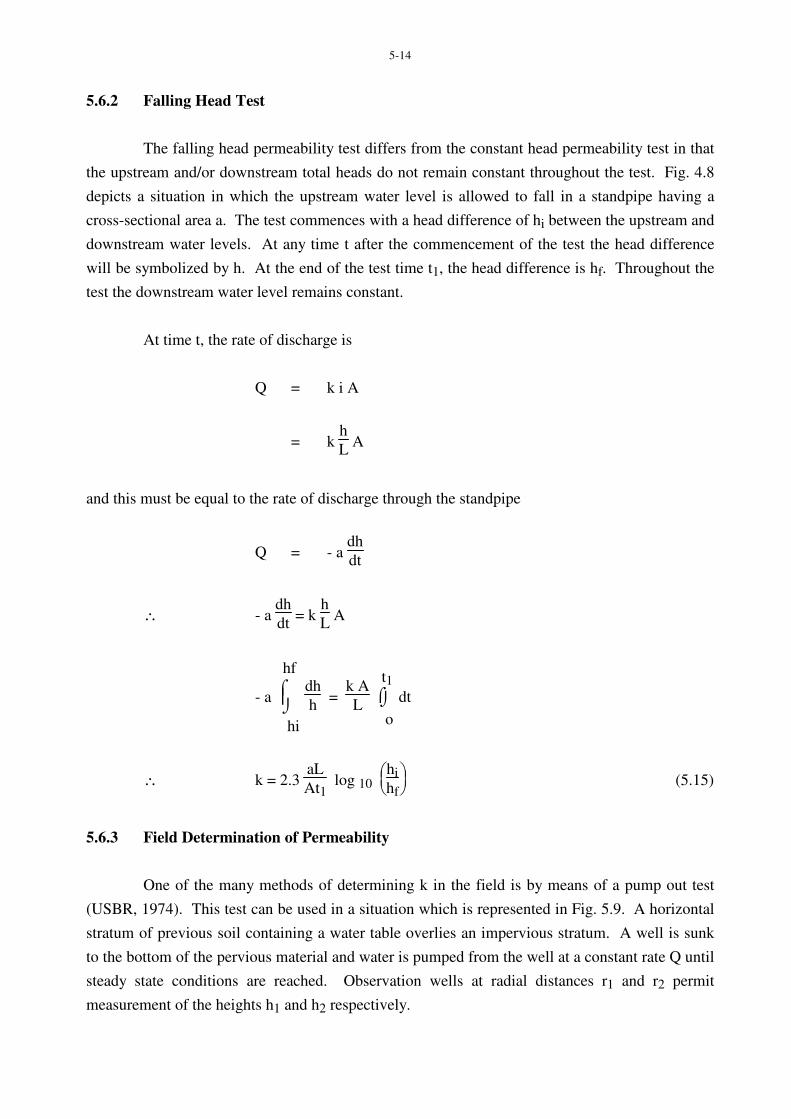
Fig. 5.10 Pump Out Test in a Confined Aquifer

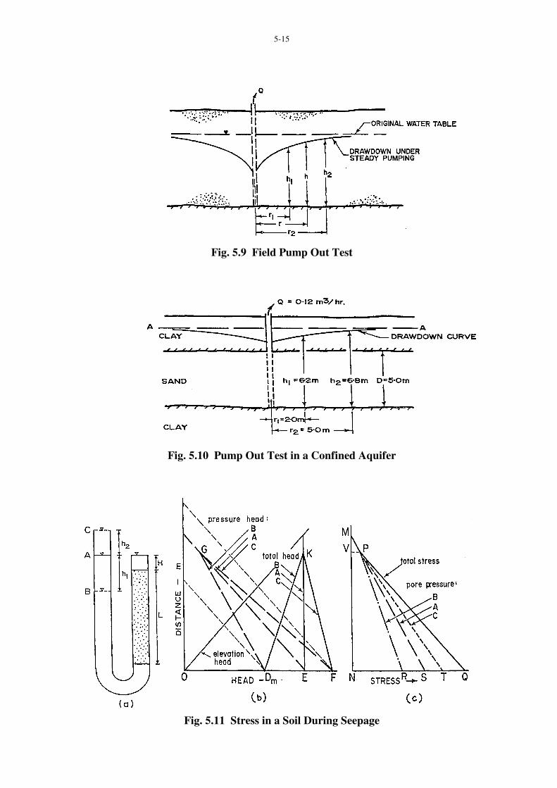
Fig. 5.11 Stress in a Soil During Seepage

5-16

At a radial distance r the cylindrically shaped area across which discharge occurs towards

the well is

A = 2 π r h

and the hydraulic gradient at this radial distance may be approximated by

i = dh

dr

applying Darcy’s law

Q = k i A

= k dh

dr 2π r h

∴ ⌡⌠

r1

r2dr

r =

2π k

Q ⌡⌠

h1

h2

hdh

lne r2

r1 =

π k (h2 2 - h1 2)

Q

∴ k = 2.3 Q log10 (r2/r1)

π (h2 2 - h1 2) (4.16)

EXAMPLE

Fig. 5.10 represents a confined sand stratum located between two relatively impermeable

clay strata. The piezometric surface (the level to which water would rise in a standpipe or

piezometric tube placed in the sand stratum) is indicated by line AA. A pump out test with

constant discharge is performed with a fully penetrating well. Observations of drawdown (steady

state conditions) at two observation wells are shown in the figure. Determine the coefficient of

permeability for the sand stratum, assuming it is homogeneous and istotropic.

Equation (5.16) cannot be used in this case since it was derived for an “unconfined”

aquifer, whereas Fig. 5.10 represents a “confined” aquifer. Consequently, the appropriate

equation will need to be derived.

5-17

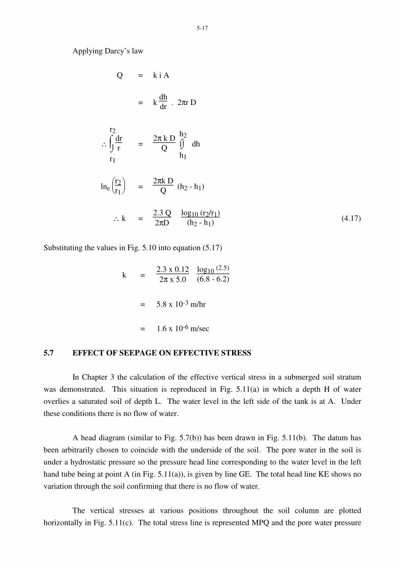
Applying Darcy’s law

Q = k i A

= k dh

dr . 2πr D

∴ ⌡⌠

r1

r2dr

r =

2π k D

Q ⌡⌠

h1

h2

dh

lne r2

r1 =

2πk D

Q (h2 - h1)

∴ k = 2.3 Q

2πD

log10 (r2/r1)

(h2 - h1) (4.17)

Substituting the values in Fig. 5.10 into equation (5.17)

k = 2.3 x 0.12

2π x 5.0

log10 (2.5)

(6.8 - 6.2)

= 5.8 x 10-3 m/hr

= 1.6 x 10-6 m/sec

5.7 EFFECT OF SEEPAGE ON EFFECTIVE STRESS

In Chapter 3 the calculation of the effective vertical stress in a submerged soil stratum

was demonstrated. This situation is reproduced in Fig. 5.11(a) in which a depth H of water

overlies a saturated soil of depth L. The water level in the left side of the tank is at A. Under

these conditions there is no flow of water.

A head diagram (similar to Fig. 5.7(b)) has been drawn in Fig. 5.11(b). The datum has

been arbitrarily chosen to coincide with the underside of the soil. The pore water in the soil is

under a hydrostatic pressure so the pressure head line corresponding to the water level in the left

hand tube being at point A (in Fig. 5.11(a)), is given by line GE. The total head line KE shows no

variation through the soil confirming that there is no flow of water.

The vertical stresses at various positions throughout the soil column are plotted

horizontally in Fig. 5.11(c). The total stress line is represented MPQ and the pore water pressure

5-18

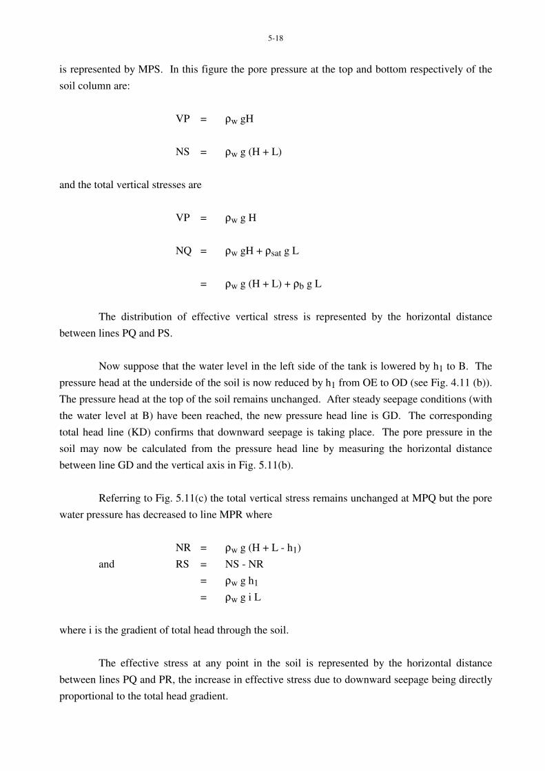
is represented by MPS. In this figure the pore pressure at the top and bottom respectively of the

soil column are:

VP = ρw gH

NS = ρw g (H + L)

and the total vertical stresses are

VP = ρw g H

NQ = ρw gH + ρsat g L

= ρw g (H + L) + ρb g L

The distribution of effective vertical stress is represented by the horizontal distance

between lines PQ and PS.

Now suppose that the water level in the left side of the tank is lowered by h1 to B. The

pressure head at the underside of the soil is now reduced by h1 from OE to OD (see Fig. 4.11 (b)).

The pressure head at the top of the soil remains unchanged. After steady seepage conditions (with

the water level at B) have been reached, the new pressure head line is GD. The corresponding

total head line (KD) confirms that downward seepage is taking place. The pore pressure in the

soil may now be calculated from the pressure head line by measuring the horizontal distance

between line GD and the vertical axis in Fig. 5.11(b).

Referring to Fig. 5.11(c) the total vertical stress remains unchanged at MPQ but the pore

water pressure has decreased to line MPR where

NR = ρw g (H + L - h1)

and RS = NS - NR

= ρw g h1

= ρw g i L

where i is the gradient of total head through the soil.

The effective stress at any point in the soil is represented by the horizontal distance

between lines PQ and PR, the increase in effective stress due to downward seepage being directly

proportional to the total head gradient.

5-19

At the base of the soil column

σ ' = NQ - NR

= ρb g L + ρw g h1

= ρb g L + ρw g i L

and at any depth z below the top of the soil

σ ' = ρb g z + ρw g i z (5.18)

The first term of this expression is due solely to the buoyant density of the soil and the

second term is caused by the seepage force.

If steady upward seepage in the soil is to occur the water level in the left side of the tank

in Fig. 4.11(a) may be raised to C. In this case the pressure head at the base of the soil column is

increased by h2 from OE to OF (see Fig. 5.11(b)). The new pressure head line becomes GF. The

new total head line becomes KF confirming that upward seepage is taking place. As before, the

pore water pressure in the soil may be calculated from the pressure head which is given by the

horizontal distance between the vertical axis and the pressure head line GF. This increased pore

pressure is indicated in Fig. 4.11(c) by the horizontal distance between the vertical axis and line

PT.

NT = ρw g (H + L + h2)

The effective vertical stress is represented by the horizontal distance between lines PQ

and PT. The effective stress at any depth z below the top of the soil may be shown to be

σ ' = ρb g z - ρw g i z (5.19)

From the above presentation it is evident that effective stress in a soil, through which

seepage is occurring, may be determined by two alternative methods

(a) by consideration of total stresses and pore pressures, or

(b) by consideration of buoyant density and seepage force.

5-20

The effective stress becomes zero when (from equation (5.19))

ρb = ρw i

or i = ρb

ρw = ic (5.20)

This particular value of the gradient is referred to as the critical gradient and when this

state is reached in a sand the pheomenon known as quicksand develops. Because the effective

stress is zero the sand possesses no strength so the soil behaves as a dense fluid.

EXAMPLE

If the sand in Fig. 5.11(a) has a specific gravity (G) of 2.65 and a void ratio (e) of 0.5

determine the critical gradient at which a quicksand condition develops.

If may be shown (for example, by use of the phase diagram) that

ρb = (G-1)

1 + e ρw

∴ ic = ρb

ρw =

G - 1

1 + e

= 2.65 - 1

1 + 0.5

= 1.1

5.8 THE FLOW NET

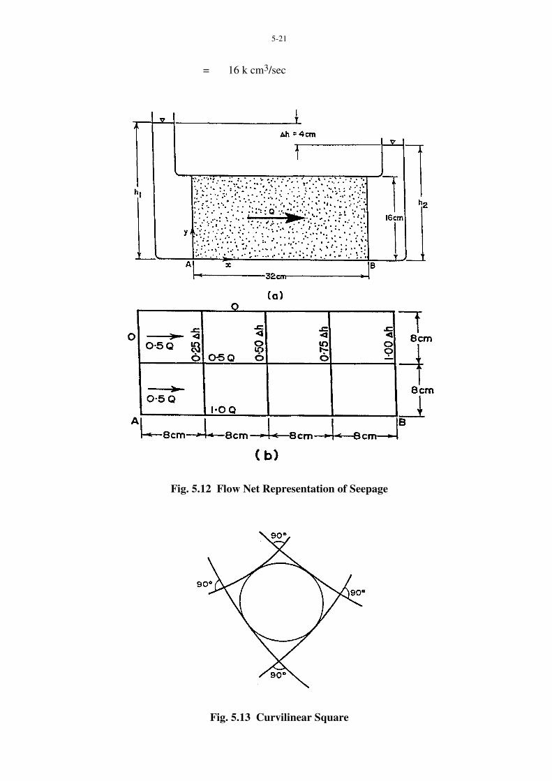
Fig. 5.12(a) represents a one dimensional steady state seepage situation under constant

head conditions. The soil is contained in a tank of rectangular section measuring 16 cm high by

8cm wide. The loss in total head through the soil (_h) is equal to 4cm. The rate of seepage flow

(Q) can be expressed in terms of the permeability, k cm/sec.

Q = k i A (5.4)

= k x 4

32 x 16 x 8

5-21

= 16 k cm3/sec

Fig. 5.12 Flow Net Representation of Seepage

Fig. 5.13 Curvilinear Square

5-22

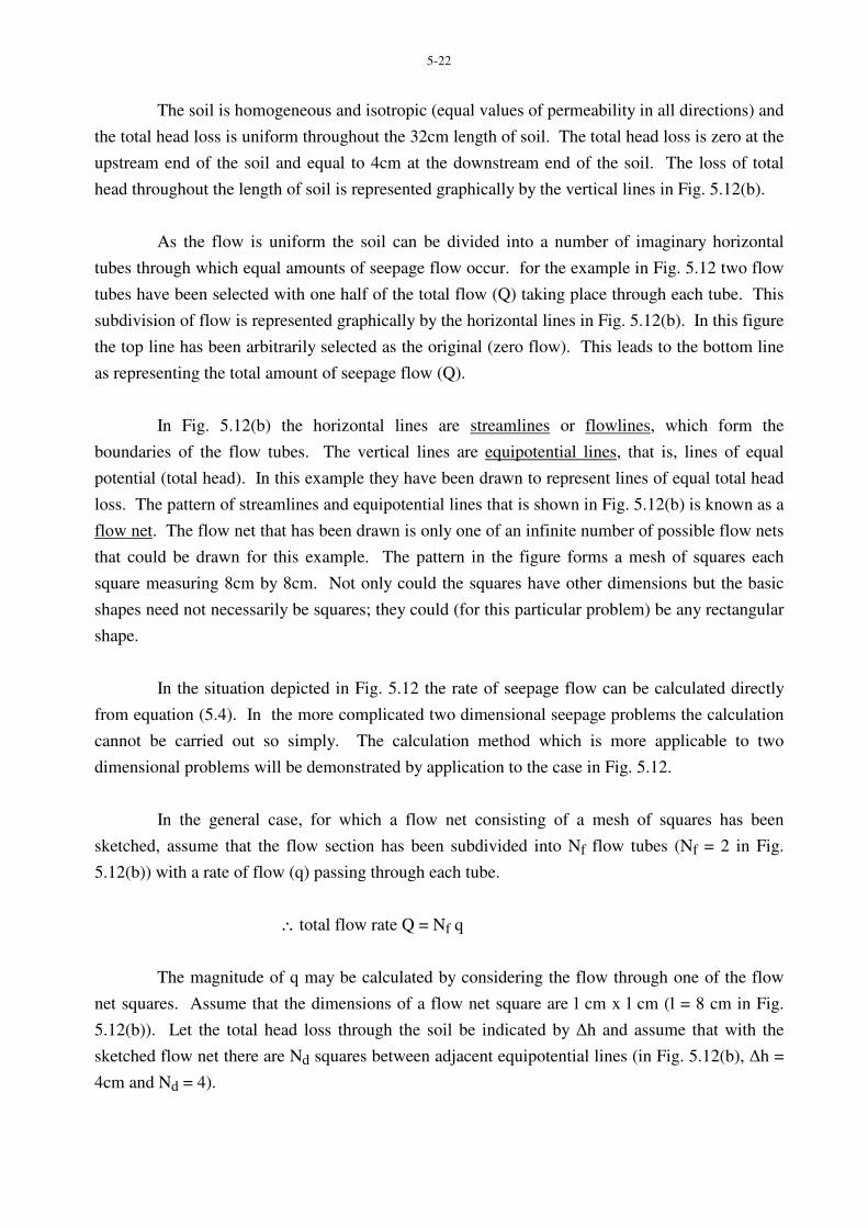
The soil is homogeneous and isotropic (equal values of permeability in all directions) and

the total head loss is uniform throughout the 32cm length of soil. The total head loss is zero at the

upstream end of the soil and equal to 4cm at the downstream end of the soil. The loss of total

head throughout the length of soil is represented graphically by the vertical lines in Fig. 5.12(b).

As the flow is uniform the soil can be divided into a number of imaginary horizontal

tubes through which equal amounts of seepage flow occur. for the example in Fig. 5.12 two flow

tubes have been selected with one half of the total flow (Q) taking place through each tube. This

subdivision of flow is represented graphically by the horizontal lines in Fig. 5.12(b). In this figure

the top line has been arbitrarily selected as the original (zero flow). This leads to the bottom line

as representing the total amount of seepage flow (Q).

In Fig. 5.12(b) the horizontal lines are streamlines or flowlines, which form the

boundaries of the flow tubes. The vertical lines are equipotential lines, that is, lines of equal

potential (total head). In this example they have been drawn to represent lines of equal total head

loss. The pattern of streamlines and equipotential lines that is shown in Fig. 5.12(b) is known as a

flow net. The flow net that has been drawn is only one of an infinite number of possible flow nets

that could be drawn for this example. The pattern in the figure forms a mesh of squares each

square measuring 8cm by 8cm. Not only could the squares have other dimensions but the basic

shapes need not necessarily be squares; they could (for this particular problem) be any rectangular

shape.

In the situation depicted in Fig. 5.12 the rate of seepage flow can be calculated directly

from equation (5.4). In the more complicated two dimensional seepage problems the calculation

cannot be carried out so simply. The calculation method which is more applicable to two

dimensional problems will be demonstrated by application to the case in Fig. 5.12.

In the general case, for which a flow net consisting of a mesh of squares has been

sketched, assume that the flow section has been subdivided into Nf flow tubes (Nf = 2 in Fig.

5.12(b)) with a rate of flow (q) passing through each tube.

∴ total flow rate Q = Nf q

The magnitude of q may be calculated by considering the flow through one of the flow

net squares. Assume that the dimensions of a flow net square are l cm x l cm (l = 8 cm in Fig.

5.12(b)). Let the total head loss through the soil be indicated by ∆h and assume that with the

sketched flow net there are Nd squares between adjacent equipotential lines (in Fig. 5.12(b), ∆h =

4cm and Nd = 4).

5-23

∴ Total head loss per square = ∆h

Nd

Total head gradient through the square i = ∆h

Nd1

Using the Darcy expression

q = k i A (5.4)

= k. ∆h

Nd1 . l.l per unit width

= k ∆h

Nd per unit width

Total flow rate Q = N f q

= k ∆h Nf

Nd per unit width (5.21)

For the problem in Fig. 4.12

q = k x 4 x 2

4

= 2 k cm3/sec. per unit width

= 2 k x 8

= 16 k cm3/sec.

in agreement with the calculation on page 5.17.

Equation (5.21) can be used in more general two dimensional flow situations in which

the direct application of equation (5.4) is not appropriate.

5.9 FLOW IN TWO DIMENSIONS

In two dimensional flow problems the equipotential lines and flowlines are generally

curved, but they intersect each other everywhere at right angles (see section 5.11). The flow net

may be determined by one of a number of techniques; such as by mathematical calculation, by

relaxation, finite difference or finite element techniques, by physical models or by manual trial

and error sketching. Some of these techniques have been discussed by Halek and Svec (1979) and

5-24

by Huyakorn and Pinder (1983). If the flow net is sketched the square shapes illustrated in Fig.

5.12(b) become distorted into "curvilinear" squares. A curvilinear square as shown in Fig. 5.13 in

a shape in which the four sides intersect at right angles and within which a circle touching all

sides may be inscribed. In the limit, as the size becomes smaller and smaller a curvilinear square

becomes an exact square.

EXAMPLE

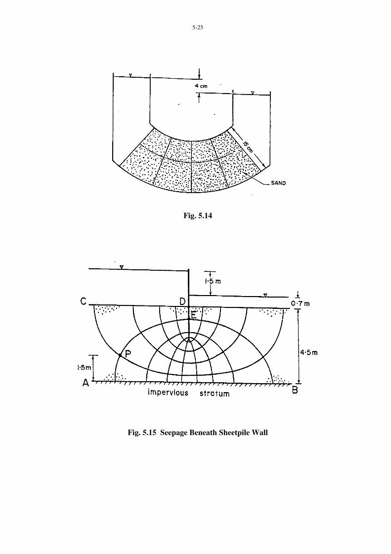
A curved box of rectangular cross section (15 cm x 3 cm) is filled with sand as illustrated

in Fig. 5.14. Steady state seepage through the sand is produced under constant head conditions.

If the sand permeability is 1.8 x 10-5m/sec determine the rate of seepage discharge.

If an attempt is made to solve this problem by means of equation (5.4) it is found that the

total head gradient i cannot be evaluated with confidence since the length over which the total

head loss of 4 cm occurs is not constant but depends upon the particular streamline selected. It is

apparent that equation (5.21) must be used (with a square mesh flow net).

From the flow net, which has been drawn in Fig. 5.14 the numbers of flow tubes and

equipotential drops may be determined for substitution into equation (5.21).

Q per unit width = k∆h Nf

Nd (5.21)

= 1.8 x 10-5 x 102 x 4 x 2

4

= 3.6 x 10-3cm3/sec/cm width

Total Q = 3.6 x 10-3 x 3

= 10.8 x 10-3 cm3/sec

EXAMPLE

Fig. 5.15 represents flow beneath a sheet piling wall. This flow net has been drawn by

trial and error manual sketching. Determine:

(a) the pore water pressure at point P, and

(b) the maximum exit gradient

5-25

Fig. 5.14

Fig. 5.15 Seepage Beneath Sheetpile Wall

5-26

(a) The total head difference of 1.5m between the upstream and downstream sides of the

sheeting piling is lost over nine equipotential drops for the flow net that is drawn. If the

impervious boundary AB is aribitrarily chosen as datum then the total head for the equipotential

line CD along the upstream boundary of the flow region may be calculated.

total head for CD = elevation head + pressure head

= 4.5 + 2.2

= 6.7m

The total head for the equipotential line passing through point P is less than this 6.7m by

the amount of total head lost in one equipotential drop.

total head for equipotential line through P

= 6.7 - 1.5

9

= 6.53m

This means that the total head for every point on the equipotential line passing through

point P is 6.53m. For point P in particular the elevation head is 1.5m.

∴ pressure head at point P = total head - elevation head

= 6.53 - 1.5

= 5.03m

∴ pore pressure = 5.03 x 9.81 x 1000 N/m2

= 49.4 kN/m2

(b) The exit gradient will be calculated for the last equipotential drop in the flow net in Fig.

5.15.

total head loss = 1.5

9 = 0.17m.

5-27

The length over which this head is lost varies with the flow line considered and increases

with increasing distance from the sheet pile. The minimum length is immediately adjacent to the

sheet pile, that is, distance DE which measures 0.75m from the flow net.

∴ maximum gradient = 0.17

0.75

= 0.22

EXAMPLE

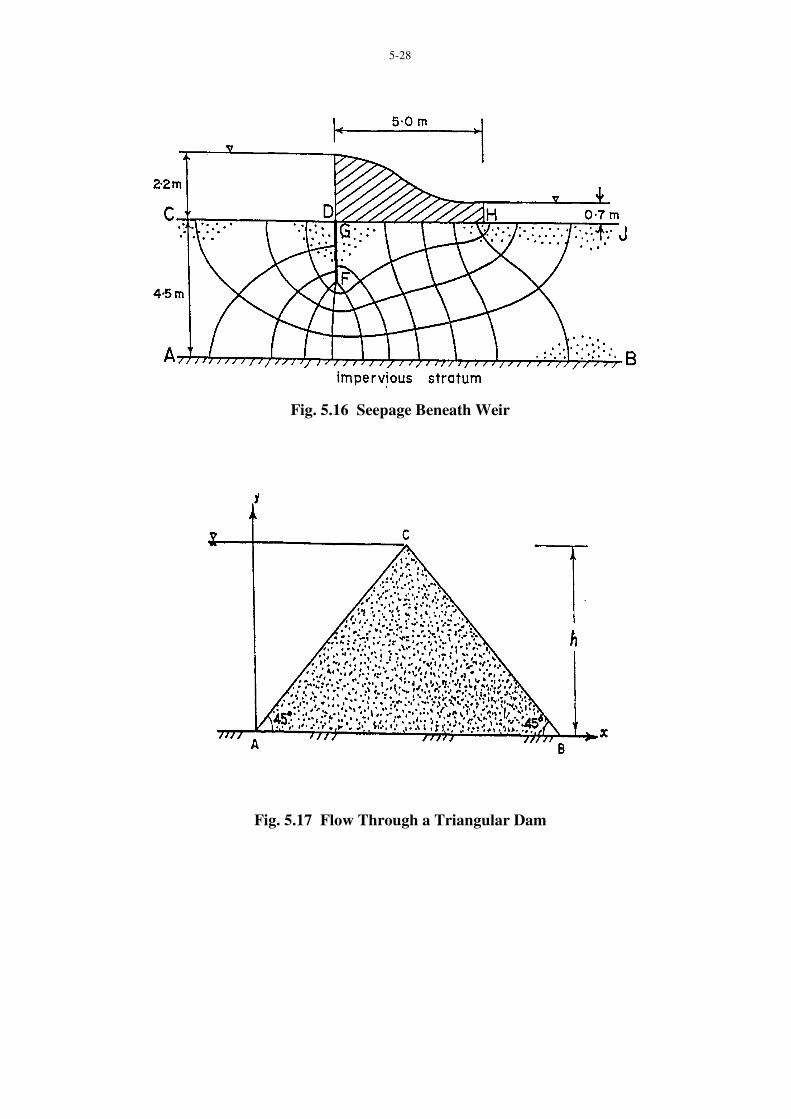
Suppose that a weir 5m long with a cutoff wall as illustrated in Fig. 4.16 is to be

considered as an alternative to the sheet pile wall in Fig. 4.15. Sketch the flow net for the new

geometry and compare the rate of seepage discharge for this case with that depicted in Fig. 4.15.

The permeability of the sand may be taken as 5µ m/sec.

In sketching the flow net in Fig. 4.16 the following points need to be remembered:

(a) All flow lines commence on the upstream equipotential line CD and terminate on the

downstream equipotential line HJ with right angle intersections.

(b) DFGH and AB are flowlines.

(c) All equipotential lines must intersect the two flowlines identified in (b) as well as every

other flowline at right angles.

(d) No two flowlines should touch each other.

(e) No two equipotential lines should touch each other.

Suggestions for the beginner in learning graphical sketching of flownets have been given

by Casagrande (1937) and Cedergren (1977). Using equation (4.21) for the flownet sketched in

Fig. 5.16:

Q = k∆h Nf

Nd

= 5 x 10-6 x 1.5 x 4

11

= 2.73 x 10-6 m3/sec for unit width.

5-28

Fig. 5.16 Seepage Beneath Weir

Fig. 5.17 Flow Through a Triangular Dam

5-29

By comparison, for the sheet pile wall in Fig. 5.15

Q = 5 x 10-6 x 1.5 x 4.5

9

= 3.75 x 10-6 m3/sec per unit width

indicating that a slightly greater rate of underseepage occurs with the sheet pile wall.

REFERENCES

Bowles, J.E., (1970), “Engineering Properties of Soils and Their Measurement”, McGraw Hill

Book Co., New York.

Casagrande, A., “Seepage through Dams” Jnl. New England Water Works Assn., Vol. 51, No. 2,

June 1937, also published in “Contributions to Soil Mechanics, 1925-1940”, Boston Society of

Civil Engineers, pp 295-336, 1940.

Cedergren, H.R., (1977) “Seepage, Drainage and Flow Nets”, John Wiley and Sons, New York,

534p.

Halek, V. and Svec, J., (1979), “Groundwater Hydraulics” Elsevier, Amsterdam, 620p.

Harr, M.E., (1962) “Groundwater and Seepage”, McGraw-Hill, New York, 315p.

Huyakorn, P.S. and Pinder, G.F., (1983), “Computational Methods in Subsurface Flow”,

Academic Press, New York, 473p.

Lambe, T.W., and Whitman, R.V., (1979), “Soil Mechanics SI Version”, John Wiley and Sons,

New York, 553p.

Lambe, T.W., (1951), “Soil Testing for Engineers”, John Wiley and Sons, New York, 165p.

Mitchell, J.K. (1976), “Fundamental of Soil Behaviour”, John Wiley and Sons, New York.

Olsen, H.W., (1962) “Hydraulic Flow through Saturated Clays”, Proc. Ninth National Conference

on Clays and Clay Minerals, pp 131 - 161.

United States Bureau of Reclamation, (1974) “Earth Manual”, Dept. of the Interior, 810p.