4 · web viewchapter 5 diffusion in solids 5.1 diffusion in nuclear processes 1 5.2. macroscopic...
TRANSCRIPT
Chapter 5 Diffusion in Solids
5.1 Diffusion in Nuclear Processes..............................................................................15.2. Macroscopic View of Diffusion..............................................................................2
Species Conservation...............................................................................................2Fick’s Laws...............................................................................................................3
5.3 Useful Mathematical Solutions...............................................................................4Constant-Source Method..........................................................................................4Instantaneous Source Method..................................................................................7Diffusion in Finite Solids............................................................................................7Fission Gas Release from Nuclear Fuel...................................................................9
5.4. Atomic Mechanisms of Diffusion in Solids.........................................................10The Einstein Equation.............................................................................................15The Vacancy Mechanism in Metals........................................................................17
5.5. Types of Diffusion Coefficients...........................................................................19Relations between the Types of Diffusion Coefficients...........................................20
5.6. Diffusion in Ionic Crystals....................................................................................21The NaCl-type Structure with Schottky Defects......................................................22
5.7. Diffusion in the Fluorite Structure of UO2...........................................................24Oxygen Diffusion.....................................................................................................24Uranium Diffusion...................................................................................................27Uranium Self-Diffusion in UO2.................................................................................28Interdiffusion in Mixed Ionic Solids with the Fluorite Structure................................32
5.8. Thermal Diffusion..................................................................................................35Appendix 5A Dimensionless Variables and the Similarity Transformation Solution to Eq s (5.4) – (5.7).....................................................................................38Appendix 5B Laplace Transform Solution to Eqs (5.16) – (5.18).........................40
Problems.......................................................................................................................42References....................................................................................................................46
Light Water Reactor Materials, Draft 2006 © Donald Olander and Arthur Motta 5/16/2023 1
1
1
5.1 Diffusion in Nuclear Processes
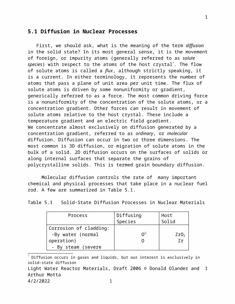
First, we should ask, what is the meaning of the term diffusion in the solid state? In its most general sense, it is the movement of foreign, or impurity atoms (generally referred to as solute species) with respect to the atoms of the host crystal*. The flow of solute atoms is called a flux, although strictly speaking, it is a current. In either terminology, it represents the number of atoms that pass a plane of unit area per unit time. The flux of solute atoms is driven by some nonuniformity or gradient, generically referred to as a force. The most common driving force is a nonuniformity of the concentration of the solute atoms, or a concentration gradient. Other forces can result in movement of solute atoms relative to the host crystal. These include a temperature gradient and an electric field gradient. We concentrate almost exclusively on diffusion generated by a concentration gradient, referred to as ordinary, or molecular diffusion. Diffusion can occur in two or three dimensions. The most common is 3D diffusion, or migration of solute atoms in the bulk of a solid. 2D diffusion occurs on the surfaces of solids or along internal surfaces that separate the grains of polycrystalline solids. This is termed grain boundary diffusion.
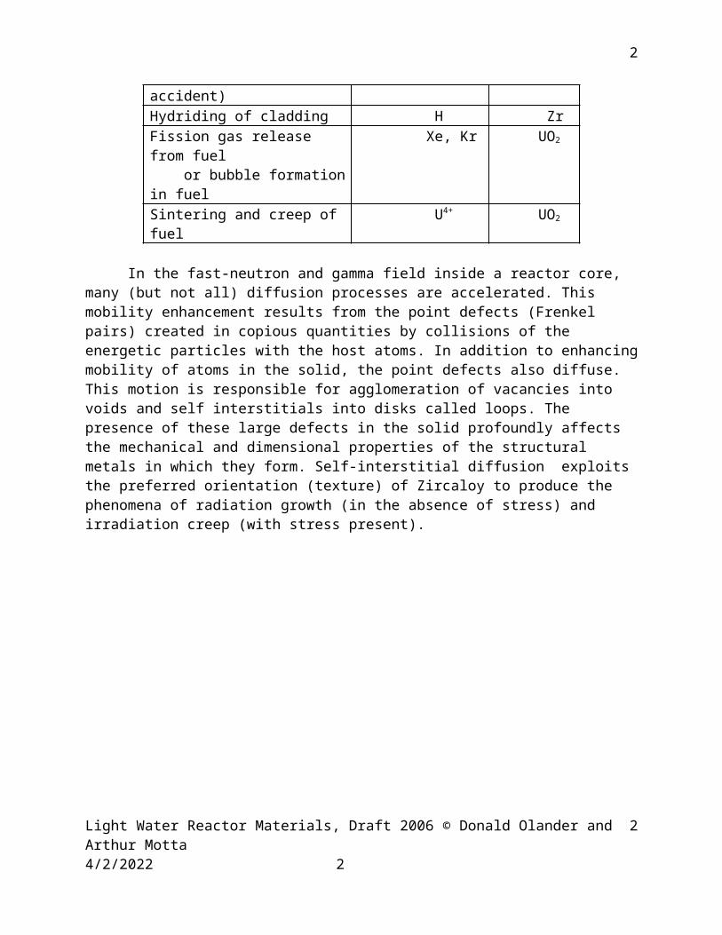
Molecular diffusion controls the rate of many important chemical and physical processes that take place in a nuclear fuel rod. A few are summarized in Table 5.1.
Table 5.1 Solid-State Diffusion Processes in Nuclear Materials
Process Diffusing Species Host SolidCorrosion of cladding: -By water (normal operation) - By steam (severe accident)
O2-
O ZrO2
ZrHydriding of cladding H ZrFission gas release from fuel or bubble formation in fuel
Xe, Kr UO2
Sintering and creep of fuel U4+ UO2
In the fast-neutron and gamma field inside a reactor core, many (but not all) diffusion processes are accelerated. This mobility enhancement results from the point defects (Frenkel pairs) created in copious quantities by collisions of the energetic particles with the host atoms. In addition to enhancing mobility of atoms in the solid, the point defects also diffuse. This motion is responsible for agglomeration of vacancies into voids and self interstitials into disks called loops. The presence of these large defects in the solid profoundly affects the mechanical and dimensional properties of the structural metals in which they form. Self-interstitial diffusion exploits the preferred orientation (texture) of Zircaloy to produce the phenomena of radiation growth (in the absence of stress) and irradiation creep (with stress present).
* Diffusion occurs in gases and liquids, but our interest is exclusively in solid-state diffusionLight Water Reactor Materials, Draft 2006 © Donald Olander and Arthur Motta 5/16/2023 1
1
1
5.2. Macroscopic View of Diffusion
Just as thermodynamics can be described from a macroscopic, classical viewpoint or in a microscopic, statistical setting, so can the process of diffusion. The macroscopic laws of diffusion are combinations of a species conservation equation with a mathematical specification of the flux of the solute relative to the host substance.
Species Conservation
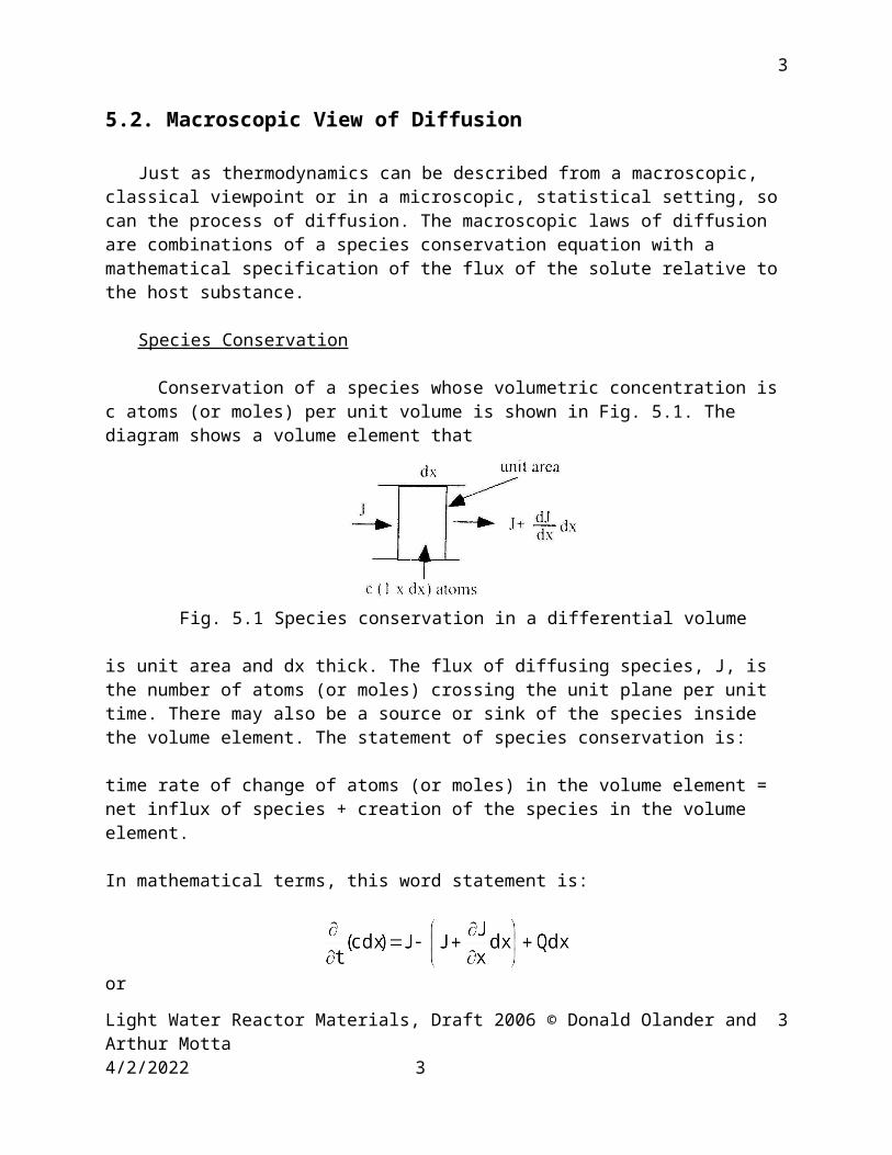
Conservation of a species whose volumetric concentration is c atoms (or moles) per unit volume is shown in Fig. 5.1. The diagram shows a volume element that
Fig. 5.1 Species conservation in a differential volume
is unit area and dx thick. The flux of diffusing species, J, is the number of atoms (or moles) crossing the unit plane per unit time. There may also be a source or sink of the species inside the volume element. The statement of species conservation is:
time rate of change of atoms (or moles) in the volume element = net influx of species + creation of the species in the volume element.
In mathematical terms, this word statement is:
or
(5.1)
where t = time x = distance Q = source term of the diffusing species, atoms (or moles) per unit volume
This conservation statement applies no matter what force is driving the flux J. The most common forces is a chemical potential gradient in the x direction. However temperature, and electric field gradients can also cause a particle flux. The three forces above lead, respectively, to fluxes describing ordinary molecular diffusion, thermal diffusion, and ionic transport.
Light Water Reactor Materials, Draft 2006 © Donald Olander and Arthur Motta 5/16/2023 2
2
2
Fick’s Laws
When the concentration gradient drives J, the flux is given by Fick’s First Law:
(5.2)
This equation follows the universal observation that matter diffuses from regions of high concentration to regions of low concentration, hence the minus sign.. The flux J and the concentration gradient are in principle measurable quantities, so Eq (5.2) effectively defines the diffusion coefficient D. The definition is not the only one possible; for example, J could have been considered to be proportional to the square of the concentration gradient. The reason that Eq (5.2) is the appropriate definition is that the quantity D is a function of temperature and concentration only, but not of the concentration gradient. Any other flux – concentration gradient relation would not have this essential property. The units of D are length squared per unit time, usually cm2/s provided that J, c, and x are in consistent units.
Substituting Eq (5.2) into Eq (5.1) gives Fick’s Second Law:
This equation is also called the diffusion equation, by analogy to its heat transport counterpart, the heat conduction equation. In the common case of an isothermal system and D independent of solute concentration(and hence of x), the diffusion equation simplifies to:
(5.3a)
If the concentration is nonuniform in the directions transverse to x, additional second derivative terms are required on the right hand side. However, mathematical solutions of multidirectional diffusion equations are considerably more complicated than those involving only one spatial dimension. Analogous equations for cylindrical and spherical geometry, involving one direction only, are:
Cylindrical geometry: (5.3b)
Spherical geometry: (5.3c)
5.3 Useful Mathematical Solutions
There are a number of analytic solutions to the time-dependent, one-spatial-dimension diffusion equation. Compendiums of such solutions are contained inn books Light Water Reactor Materials, Draft 2006 © Donald Olander and Arthur Motta 5/16/2023 3
3
3
by Carslaw and Jaeger (1) and Crank (2). Diffusion problems that are not amenable to closed-form solutions can be solved by numerical techniques¸ for which numerous computer codes are available.
Constant-Source Method
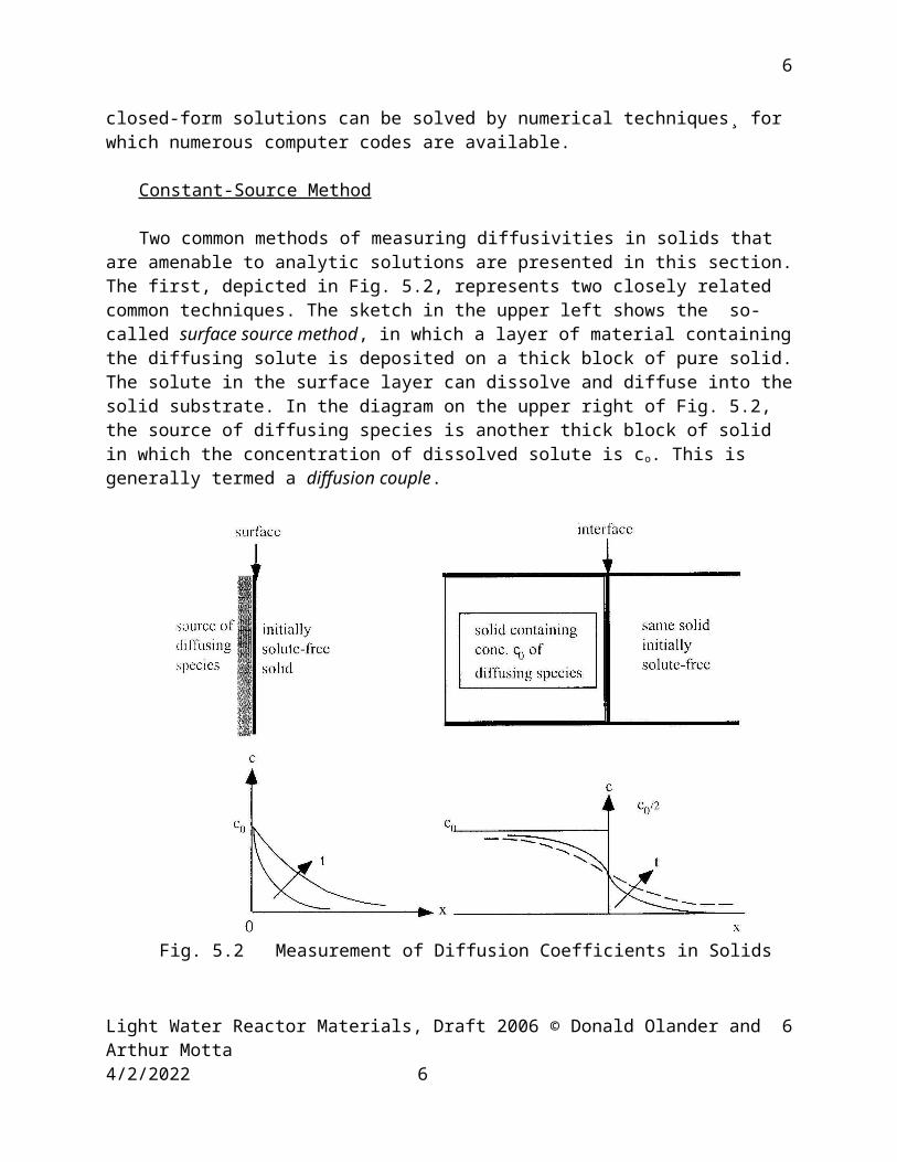
Two common methods of measuring diffusivities in solids that are amenable to analytic solutions are presented in this section. The first, depicted in Fig. 5.2, represents two closely related common techniques. The sketch in the upper left shows the so-called surface source method, in which a layer of material containing the diffusing solute is deposited on a thick block of pure solid. The solute in the surface layer can dissolve and diffuse into the solid substrate. In the diagram on the upper right of Fig. 5.2, the source of diffusing species is another thick block of solid in which the concentration of dissolved solute is co. This is generally termed a diffusion couple.
Fig. 5.2 Measurement of Diffusion Coefficients in Solids
For ease of post-diffusion measurement of the concentration profile, the diffusing species (the solute) is often a radioisotope. In the surface source method, the surface layer is assumed be a pure species which has a known solubility in the substrate. Instead of a surface layer, the source of the diffusing species may be a gas or liquid. In the couple method, the two blocks are usually the same species. The diffusing
species charged to the left hand block can either be a different element from that which comprises the two solid blocks or an isotope of the host-element species. For simplicity
Light Water Reactor Materials, Draft 2006 © Donald Olander and Arthur Motta 5/16/2023 4
4
4
of analysis, the latter is assumed, so the quantity measured in the experiment is the self-diffusion coefficient.
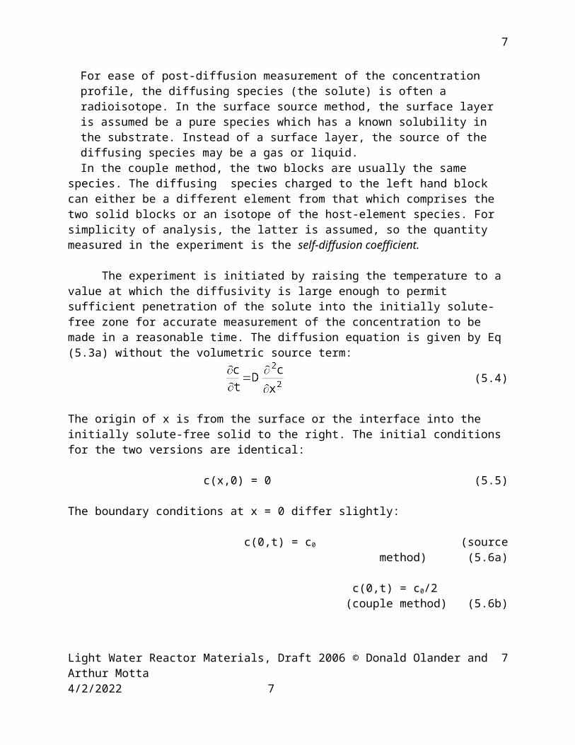
The experiment is initiated by raising the temperature to a value at which the diffusivity is large enough to permit sufficient penetration of the solute into the initially solute-free zone for accurate measurement of the concentration to be made in a reasonable time. The diffusion equation is given by Eq (5.3a) without the volumetric source term:
(5.4)
The origin of x is from the surface or the interface into the initially solute-free solid to the right. The initial conditions for the two versions are identical:
c(x,0) = 0 (5.5)
The boundary conditions at x = 0 differ slightly:
c(0,t) = c0 (source method) (5.6a)
c(0,t) = c0/2 (couple method) (5.6b)
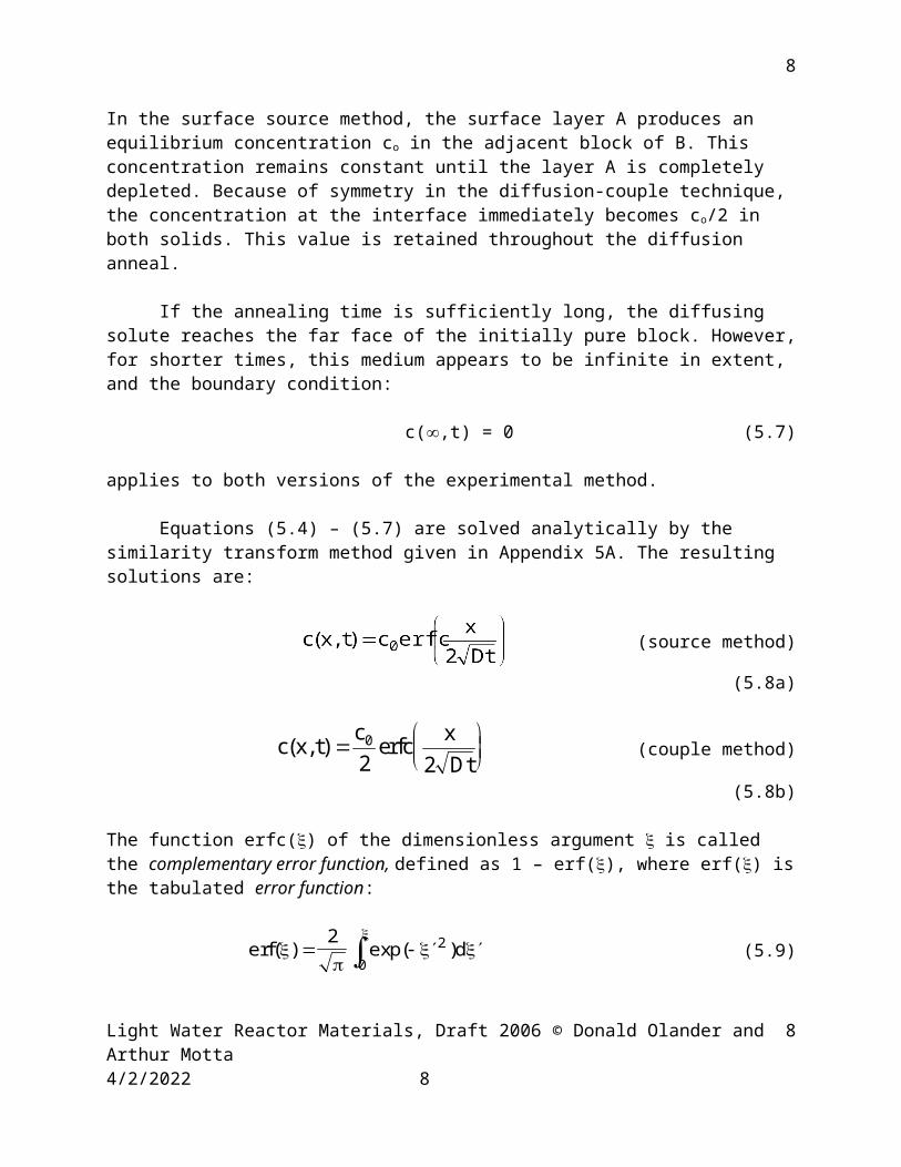
In the surface source method, the surface layer A produces an equilibrium concentration co in the adjacent block of B. This concentration remains constant until the layer A is completely depleted. Because of symmetry in the diffusion-couple technique, the concentration at the interface immediately becomes co/2 in both solids. This value is retained throughout the diffusion anneal.
If the annealing time is sufficiently long, the diffusing solute reaches the far face of the initially pure block. However, for shorter times, this medium appears to be infinite in extent, and the boundary condition:
c(,t) = 0 (5.7)
applies to both versions of the experimental method.
Equations (5.4) – (5.7) are solved analytically by the similarity transform method given in Appendix 5A. The resulting solutions are:
(source method) (5.8a)
c x tcerfc x
Dt( , )
0
2 2 (couple method) (5.8b)
Light Water Reactor Materials, Draft 2006 © Donald Olander and Arthur Motta 5/16/2023 5
5
5
The function erfc() of the dimensionless argument is called the complementary error function, defined as 1 – erf(), where erf() is the tabulated error function:
erf( ) exp( )d
2 2
0(5.9)
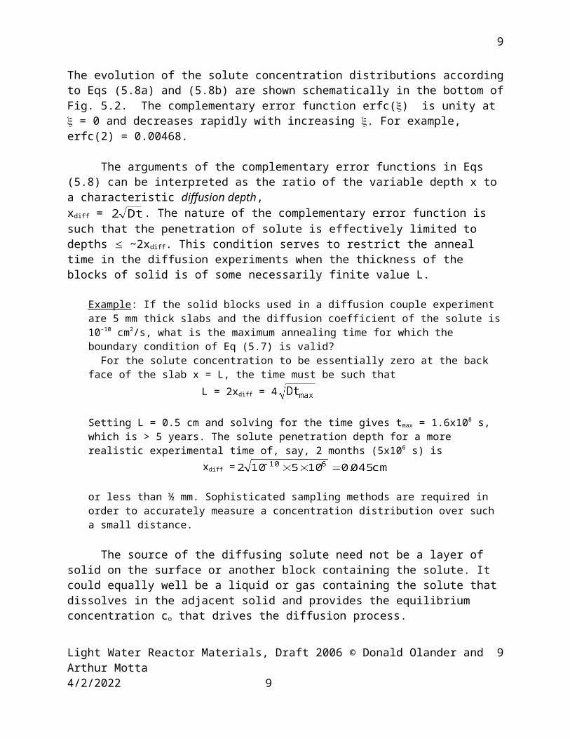
The evolution of the solute concentration distributions according to Eqs (5.8a) and (5.8b) are shown schematically in the bottom of Fig. 5.2. The complementary error function erfc() is unity at = 0 and decreases rapidly with increasing . For example, erfc(2) = 0.00468.
The arguments of the complementary error functions in Eqs (5.8) can be interpreted as the ratio of the variable depth x to a characteristic diffusion depth,xdiff = . The nature of the complementary error function is such that the penetration of solute is effectively limited to depths ~2xdiff. This condition serves to restrict the anneal time in the diffusion experiments when the thickness of the blocks of solid is of some necessarily finite value L.
Example: If the solid blocks used in a diffusion couple experiment are 5 mm thick slabs and the diffusion coefficient of the solute is 10-10 cm2/s, what is the maximum annealing time for which the boundary condition of Eq (5.7) is valid?
For the solute concentration to be essentially zero at the back face of the slab x = L, the time must be such that
L = 2xdiff = 4
Setting L = 0.5 cm and solving for the time gives tmax = 1.6x10⁸ s, which is > 5 years. The solute penetration depth for a more realistic experimental time of, say, 2 months (5x10⁶ s) is
xdiff =
or less than ½ mm. Sophisticated sampling methods are required in order to accurately measure a concentration distribution over such a small distance.
The source of the diffusing solute need not be a layer of solid on the surface or another block containing the solute. It could equally well be a liquid or gas containing the solute that dissolves in the adjacent solid and provides the equilibrium concentration co that drives the diffusion process.
One method of determining D from such experiments is to slice thin layers of the initially solute-free blocks and measure the concentration of solute in each layer. Alternatively, the solids can be cut to obtain a cross section perpendicular to the surface or interface. The solute concentration profile is measured by one of number of methods that use an energetic beam of highly collimated electrons or ions to excite the solute species. The radiation from decay of the excited atoms is recorded by a suitable
Light Water Reactor Materials, Draft 2006 © Donald Olander and Arthur Motta 5/16/2023 6
6
6
detector. The solute concentration profiles so obtained are fitted numerically to Eqs (5.8a) or (5.8b) to obtain the best-fitting value of D.
Instantaneous Source Method
Instead of the inexhaustible surface source that led to the solution given by Eq (5.8a), the common experimental technique involves depositing a thin layer of the diffusing species on the surface. Being a thin layer, this source contains a limited quantity of the diffusing species, and as a result, the surface concentration drops during the experiment as the source is depleted. Equations (5.4), (5.5) and (5.7) apply to this so-called instantaneous source situation, but Eq (5.6a) is not valid at the surface. In its place, the total quantity of diffusing species initially deposited on the surface and subsequently diffused into the bulk is independent of time. If M is the total quantity of diffusing species per unit area, this condition is expressed by:
(5.10)
A solution of Eq (5.4) that satisfies the initial condition Eq (5.5) and the boundary condition Eq (5.7) is c = At-1/2exp(-x2/4Dt). A is a constant that is determined by substituting this solution into Eq (5.10), which yields A = M.(D)-1/2. The final solution for the concentration profile is:
(5.11)
Diffusion in Finite Solids
When the block of solid is not thick enough to satisfy the condition
(5.12)
the boundary condition of Eq (5.7) is no longer applicable.
This change in the boundary condition completely changes the nature of the solution, and the analytic solutions of Eqs (5.8) no longer apply. The diffusion equation must be solved by the method of separation of variables and the concentration distribution expressed as an infinite series instead of the closed form represented by the complementary error function.
The solutions for one-dimensional spherical, cylindrical, and slab geometries are given by Carslaw and Jaeger (1). The equations solved are (5.3a), (5.3b) and (5.3c) without the source term Q. The origin of the distance x is the midplane of the slab instead of its surface. This permits the slab problem to be compared directly to the other two geometries, where the origin of the distance variable r is at the center of the object. The initial condition is the same as Eq (5.5), but because of the change in the origin of the distance variable, and the finite depth of the objects, the boundary conditions are:
Light Water Reactor Materials, Draft 2006 © Donald Olander and Arthur Motta 5/16/2023 7
7
7
C(L,t) = co (5.13)
Where x = L or r = L represents the surface of the slab, cylinder, or sphere.Because of symmetry, the boundary condition at the origin is:
(5.14)
For cylindrical and spherical geometries, x in this equation is replaced by r.
Figure 5.3 graphs the solutions of Eqs (5.3) subject to Eqs (5.5), (5.13) and (5.14). Shown here is the volume average concentration (relative to co) expressed in terms of the square root of the dimensionless time :
(5.15)
Fig. 5.3 Average temperatures in a slab, cylinder, and sphere
The analytic solution for the slab given by Eq (5.8a) can be regarded as a “short-time” approximation to the unrestricted results shown in Fig. 5.3.
Example A 5 mm thick slab is exposed to a source of solute for 107 s. The diffusion coefficient is 10-9 cm2/s. Compare the relative average concentration obtained from the analytical solution with that read from Fig. 5.3.
Light Water Reactor Materials, Draft 2006 © Donald Olander and Arthur Motta 5/16/2023 8
8
8
The dimensionless time is Dt/L2 = 10-9 x 10⁷/(0.5)2 = 0.05. The average concentration in the slab is M/L, where M is given by Eq (5.10):
For comparison, the appropriate curve in Fig. 5.3 is No. I. For a dimensionless time of 0.04, this curve also gives = 0.23. Although the two methods agree here, deviations begin at longer times.
Fission Gas Release from Nuclear Fuel
The physical basis of the classical model of the release of the fission gases xenon and krypton will be treated in Chap. XX. In this section, attention is restricted to the mathematical aspects of the theory as an example of the use of Fick’s second law (the diffusion equation) in spherical coordinates. Briefly, the model assumes that the rate-limiting is fission gas release is diffusion of the fission gases in the grains of uranium dioxide. The grains are assumed to be spheres of radius a. Once reaching the periphery of the grains, the fission gas is assumed to be immediately released and detected.
In a postirradiation anneal experiment designed to measure the diffusivity of the fission gases, the fuel specimen is irradiated in a neutron flux at a temperature sufficiently low that none of the gas is released. The irradiation produces a uniform concentration co in the spherical grains representing the microstructure of the solid. The specimen is then annealed at high temperature and the Xe (or Kr) escaped from the solid is trapped and measured by its radioactivity. This information yields the fraction of the fission gas released, which is the quantity that must be predicted by diffusion theory as a function of time and the diffusion coefficient.
Applying Eq (5.3a) without the volumetric source term, the diffusion equation applicable to this process is:
ct
Dr r
rcr
12
2 (5.16)
with the initial condition: c(r,0) = co (5.17)
and the boundary conditions: c(0,t) = finite; c(a,t) = 0 (5.18)
The last of these boundary conditions arises from the assumption that the gas escapes without further resistance once reaching the grain surface.
Light Water Reactor Materials, Draft 2006 © Donald Olander and Arthur Motta 5/16/2023 9
9
9
The “short-time” solution to this set is developed by the Laplace transform method in Appendix 4B. The result for the average concentration in the sphere, or alternatively, the fraction of the initial amount released is:
(5.19)
Where = Dt/a2 is the dimensionless time. Equation (5.19) can be directly compared with curve V in Fig. 5.3, which is the exact solution. The comparison is direct because of the difference in the boundary and initial conditions used in the two methods; For Fig. 5.3, the initial condition is c = 0 and the boundary condition at the periphery is c = co. In the present solution, these are reversed. Hence, from Fig. 5.3 is to be compared to the fraction release f = from Eq (5.19).
Example: For = 0.1, Eq (5.19) gives f = 0.77, which is the same as read from curve V of Fig. 5.3 at the same dimensionless time. (L is the same as a). Even though restricted to “short times”, Eq (5.19) is remarkably accurate to very large fractional releases.
5.4. Atomic Mechanisms of Diffusion in Solids
Movement of diffusing species (e.g., point defects, substitutional atoms or radioactively-tagged host atoms, interstitial impurities) relative to the host crystal ultimately depends upon the interatomic potential with which a solute atom interacts with a host atom and the analogous potential function between host atoms.
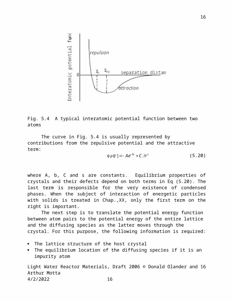
A generic interatomic potential function between a pair of atoms (or ions) is illustrated in Fig. 5.4. As the separation distance between the pair decreases, an attractive force is generated and the potential energy decreases. This attraction is the basic reason that liquids and solids exist. The attractive force may be Coulombic in nature as in ionic crystals (Chap. 2) or weak Van der Waals forces that are responsible for the condensation of the inert gases. As the atoms become close enough that their electron clouds overlap, a repulsive force develops and the potential energy increases sharply. The Pauli exclusion principle forbids two electrons from occupying the same quantum state, hence some electrons must be promoted to higher energy levels, thereby increasing the potential energy of the two-particle system.
Light Water Reactor Materials, Draft 2006 © Donald Olander and Arthur Motta 5/16/2023 10
10
10
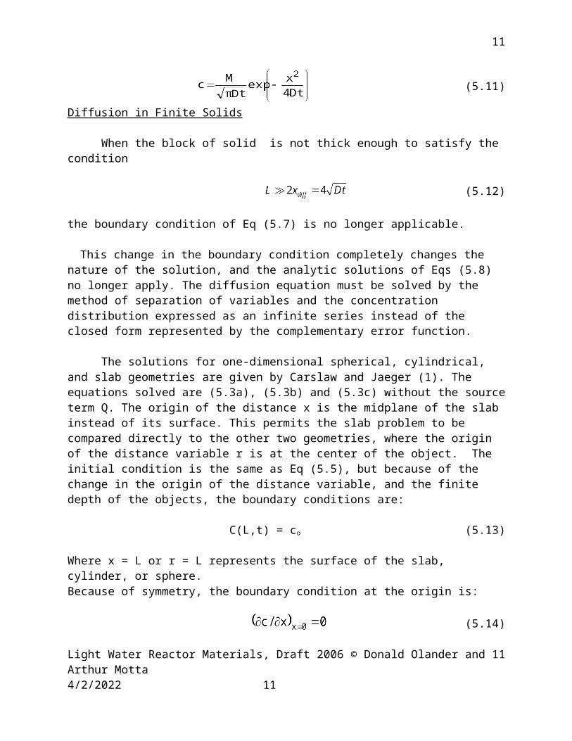
Fig. 5.4 A typical interatomic potential function between two atoms
The curve in Fig. 5.4 is usually represented by contributions from the repulsive potential and the attractive term:
(5.20)
where A, b, C and s are constants. Equilibrium properties of crystals and their defects depend on both terms in Eq (5.20). The last term is responsible for the very existence of condensed phases. When the subject of interaction of energetic particles with solids is treated in Chap.,XX, only the first term on the right is important.
The next step is to translate the potential energy function between atom pairs to the potential energy of the entire lattice and the diffusing species as the latter moves through the crystal. For this purpose, the following information is required:
The lattice structure of the host crystal The equilibrium location of the diffusing species if it is an impurity atom The path followed by the diffusing species through the lattice from one equilibrium
site to another; the diffusion path will always be the one of least resistance, specifically the route that demands the lowest average energy increase to effect the change in position, or the jump.
The temperature, which dictates the vibrational energy of all species in the system; the higher the temperature, the more likely is the diffusing species to acquire the necessary energy increment for migration.
To illustrate this procedure, the elementary case of a small impurity migrating through a simple cubic lattice is used. As shown in Fig. 5.5, the equilibrium site of the impurity atom is the center of the cube. At this position, the distance between the impurity atom and the nearest host atoms is the largest possible, which places the pair potentials at or near the separation distance req shown in Figs. 5.4 and 5.5. Because of the thermal energy shared by all atoms of the system, the impurity atom vibrates in three orthogonal [100] directions. The energy of each vibration is distributed according to a Boltzmann distribution, and very few of the vibrations possess sufficient energy to
Light Water Reactor Materials, Draft 2006 © Donald Olander and Arthur Motta 5/16/2023 11
11
11
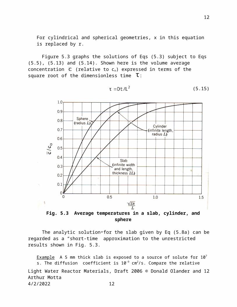
Fig. 5.5 Jump of impurity atom is crystal with sc structure
move to the adjacent equilibrium site. The required vibrational energy is the difference between the potential energy of the impurity atom at the midplane of its movement (called the barrier) and the potential energy in the equilibrium site. These two energies are obtained by summing the interactions between the impurity atom and the surrounding host atoms as a function of the x direction along which equilibrium sites and barrier planes are located. If for simplicity, we count only interactions between the impurity atom and the nearest host atoms, the system energy is:
in the equilibrium site: (5.21a)
in the barrier plane: Ub = 4(rb) (5.21b)
Even though the impurity atom has 8 nearest neighbors in the equilibrium site compared to 4 at the barrier, the pair potential at the barrier is more than twice as large as that in the equilibrium location because of the difference in the impurity-host atom distances (see Fig. 5.4).
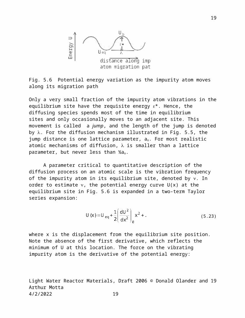
In detailed calculations of this sort, the impurity atom would be permitted to interact with host atoms further away than nearest neighbor positions, and the host atoms around the equilibrium site barrier plane would relax away from the impurity atom, thereby involving additional terms to the total energy U in these two positions. The complete potential energy variation as the impurity atom moves along the x direction is shown in Fig. 5.6. The energy barrier that must be overcome by the energy of impurity atom vibration is the difference between the peak and trough in Fig. 5.6:
* = Ub - Ueq (5.22)
Light Water Reactor Materials, Draft 2006 © Donald Olander and Arthur Motta 5/16/2023 12
12
12
Fig. 5.6 Potential energy variation as the impurity atom moves along its migration path Only a very small fraction of the impurity atom vibrations in the equilibrium site have the requisite energy *. Hence, the diffusing species spends most of the time in equilibriumsites and only occasionally moves to an adjacent site. This movement is called a jump, and the length of the jump is denoted by . For the diffusion mechanism illustrated in Fig. 5.5, the jump distance is one lattice parameter, ao. For most realistic atomic mechanisms of diffusion, is smaller than a lattice parameter, but never less than ½ao.
A parameter critical to quantitative description of the diffusion process on an atomic scale is the vibration frequency of the impurity atom in its equilibrium site, denoted by . In order to estimate , the potential energy curve U(x) at the equilibrium site in Fig. 5.6 is expanded in a two-term Taylor series expansion:
(5.23)
where x is the displacement from the equilibrium site position. Note the absence of the first derivative, which reflects the minimum of U at this location. The force on the vibrating impurity atom is the derivative of the potential energy:
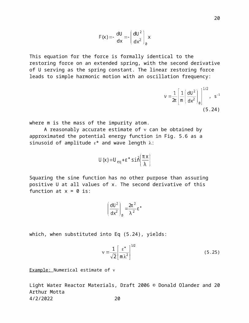
This equation for the force is formally identical to the restoring force on an extended spring, with the second derivative of U serving as the spring constant. The linear restoring force leads to simple harmonic motion with an oscillation frequency:
, s-1 (5.24)
where m is the mass of the impurity atom.A reasonably accurate estimate of can be obtained by approximated the
potential energy function in Fig. 5.6 as a sinusoid of amplitude * and wave length :
Light Water Reactor Materials, Draft 2006 © Donald Olander and Arthur Motta 5/16/2023 13
13
13
Squaring the sine function has no other purpose than assuring positive U at all values of x. The second derivative of this function at x = 0 is:
which, when substituted into Eq (5.24), yields:
12 2
1 2
m
/
(5.25)
Example: Numerical estimate of
In order to estimate , we take the mass of the diffusing atom to be that of hydrogen, a common impurity in many metals. Thus m = 10-3 kg/mole. In keeping with Fig 5.5, the jump distance is a lattice constant, or 3x10⁻¹⁰ m. There is no simple estimate of the barrier height *, theoretical knowledge of which would require a complete molecular dynamics simulation using known pair potential function such as Eq (5.20). Hence, we assume a typical value of 1 eV (~ 100 kJ/mole). Using these values in Eq (5.25) yields the impurity atom vibration frequency:
This computation makes use of the relationship for SI units J/kg = (m/s)2. The resulting = 1013 s-1 is a typical vibration frequency of atoms in a solid, including the host atoms.
The frequency at which a diffusing atom succeeds in moving from an equilibrium site to an adjacent one is much less than its vibration frequency in the equilibrium site. The vast majority of the vibrations do not possess sufficient energy to overcome the energy barrier *. The impurity atom in the position of the barrier plane is analogous to a host atom in an interstitial site. The fraction of the latter is exp(-I/kT) (Eq (3.6)). Completing the analogy, the fraction of impurity atoms in the barrier location is exp(-*/kT). Proceeding from this point to the jump frequency is accomplished by considering that the Boltzmann factor exp(-*/kT) represents the fraction of the vibrations of the impurity atom that succeed in surmounting the energy barrier *. The jump frequency is thus:
(5.26)
The preceding explanation of the origin of Eq(5.26) is appealingly simple and leads to the approximately correct result. The rigorous derivation of this equation, however, is based on
Light Water Reactor Materials, Draft 2006 © Donald Olander and Arthur Motta 5/16/2023 14
14
14
statistical mechanics and is considerably more complex than the “derivation” presented here (see Sect. 7.5 of Ref. 3).
Example: Estimate the jump frequency of an impurity atom at 1000 K with a barrier of 100 kJ/mole.
Using a vibration frequency of 1013 s-1, the jump frequency is:
or, six in a million vibrations result in a diffusional jump.
The Einstein Equation
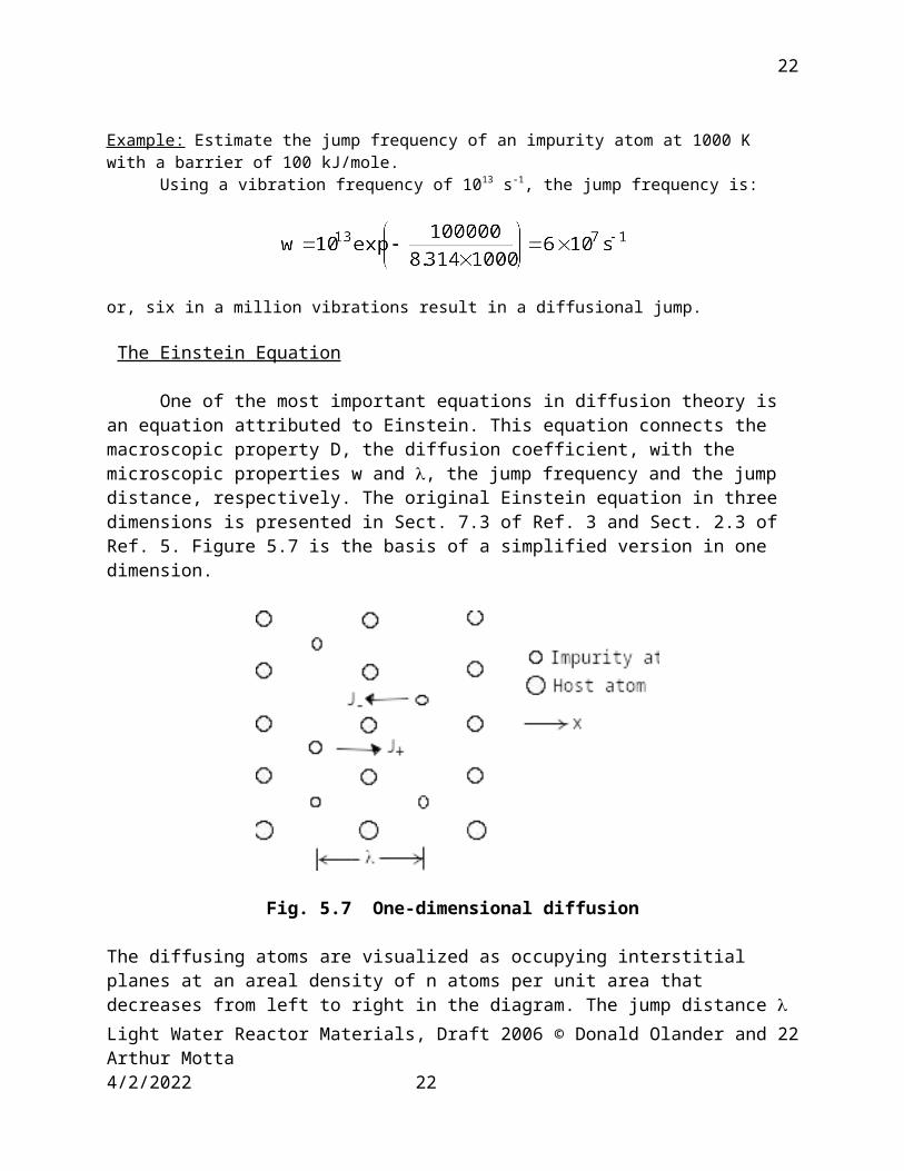
One of the most important equations in diffusion theory is an equation attributed to Einstein. This equation connects the macroscopic property D, the diffusion coefficient, with the microscopic properties w and , the jump frequency and the jump distance, respectively. The original Einstein equation in three dimensions is presented in Sect. 7.3 of Ref. 3 and Sect. 2.3 of Ref. 5. Figure 5.7 is the basis of a simplified version in one dimension.
Fig. 5.7 One-dimensional diffusion
The diffusing atoms are visualized as occupying interstitial planes at an areal density of n atoms per unit area that decreases from left to right in the diagram. The jump distance is equal to a lattice constant, so the areal density n is related to the volumetric concentration c atoms per unit volume by the equation c = n/. The rate at which impurity atoms jump from the left-hand plane to the right-hand plane is J+ = n(x)w, where w is the jump frequency. In the opposite direction, the flux is J- = n(x+)w. The net flux is:
Light Water Reactor Materials, Draft 2006 © Donald Olander and Arthur Motta 5/16/2023 15
15
15
expanding c(x+) in a one-term Taylor series about x , c(x+) = c(x)+( ), converts the flux equation to:
(5.27)
Comparison of Eq (5.27) with the macroscopic definition of the diffusion coefficient given by Eq (5.2) shows that for this one-dimensional problem,
D = 2w
The quantity w is a one-way jump frequency, or the frequency with which an impurity atom jumps from an equilibrium site to a particular adjacent equilibrium site. The frequency with which the diffusing atom jumps to any available adjacent site is called the total jump frequency, and is denoted by . In Fig. 5.7, only jumps to the left or the right are allowed, so = 2w, and the above equation becomes:
D = ½2
The exact three-dimensional analysis yields:
D = 2 (5.28)
Which is the Einstein formula. In cubic lattices, the jump distance is a fraction f of the lattice constant, or
= fao (5.29)
The total jump frequency is a multiple of the one-way jump frequency:
= w (5.30)
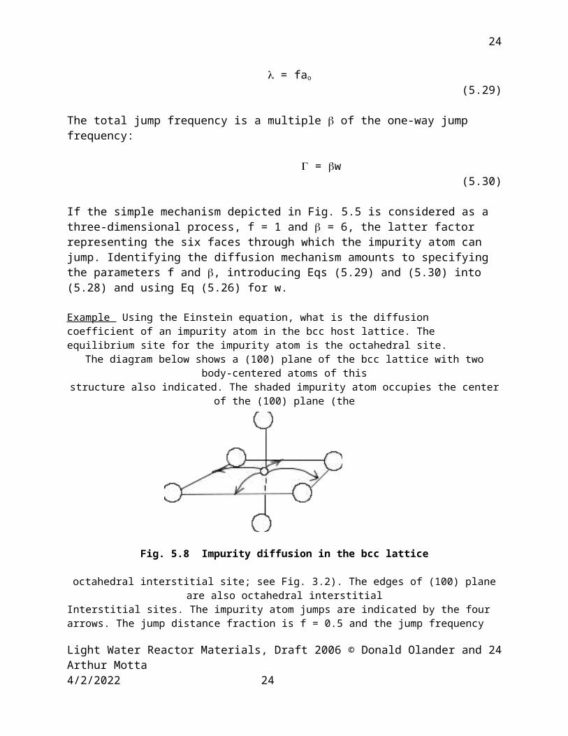
If the simple mechanism depicted in Fig. 5.5 is considered as a three-dimensional process, f = 1 and = 6, the latter factor representing the six faces through which the impurity atom can jump. Identifying the diffusion mechanism amounts to specifying the parameters f and , introducing Eqs (5.29) and (5.30) into (5.28) and using Eq (5.26) for w.
Example Using the Einstein equation, what is the diffusion coefficient of an impurity atom in the bcc host lattice. The equilibrium site for the impurity atom is the octahedral site.The diagram below shows a (100) plane of the bcc lattice with two body-centered atoms of thisstructure also indicated. The shaded impurity atom occupies the center of the (100) plane (the
Light Water Reactor Materials, Draft 2006 © Donald Olander and Arthur Motta 5/16/2023 16
16
16
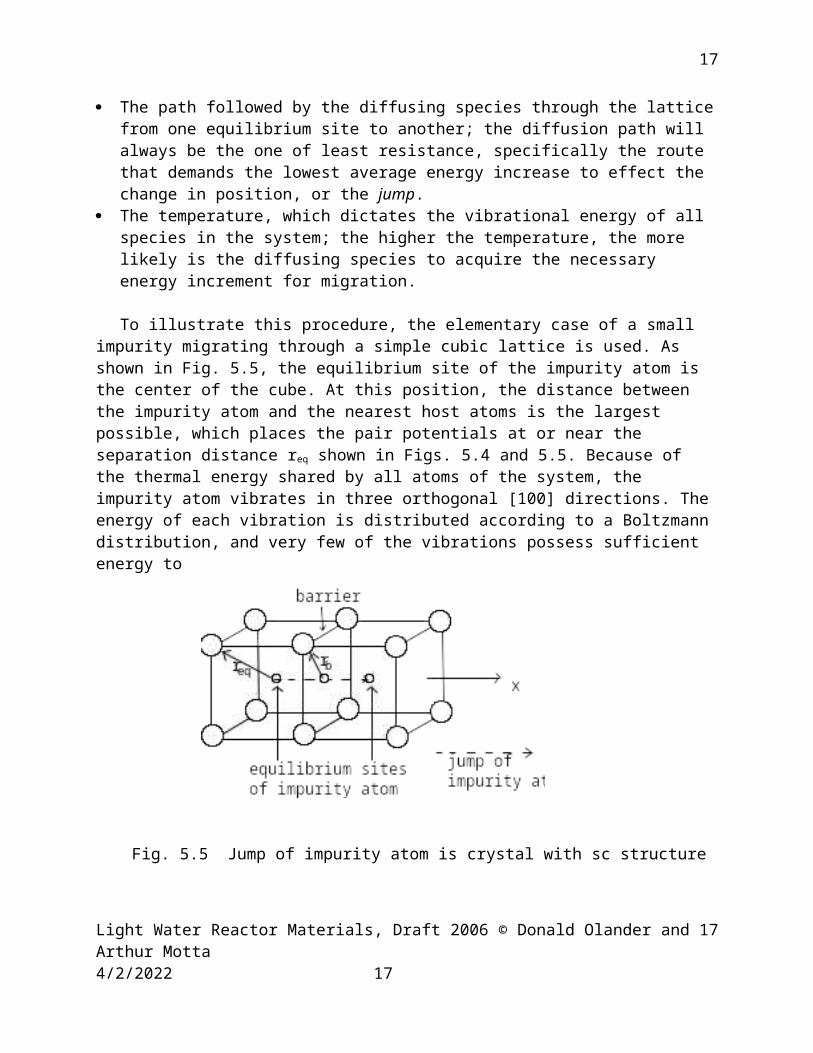
Fig. 5.8 Impurity diffusion in the bcc lattice
octahedral interstitial site; see Fig. 3.2). The edges of (100) plane are also octahedral interstitialInterstitial sites. The impurity atom jumps are indicated by the four arrows. The jump distance fraction is f = 0.5 and the jump frequency multiple is = 4. The diffusion barrier is midway along the jump in the center of a tetrahedral interstitial site (see Fig. 3.2). The diffusivity of the impurity atom is:
The Vacancy Mechanism in Metals
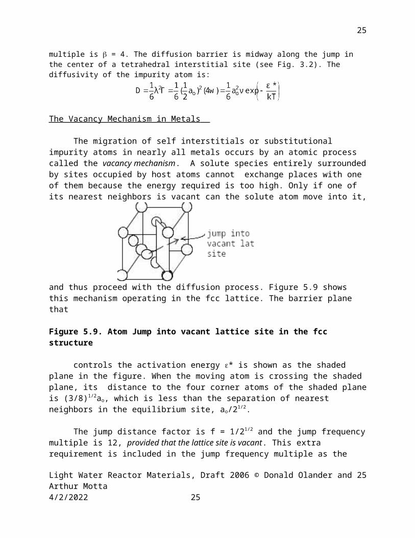
The migration of self interstitials or substitutional impurity atoms in nearly all metals occurs by an atomic process called the vacancy mechanism. A solute species entirely surrounded by sites occupied by host atoms cannot exchange places with one of them because the energy required is too high. Only if one of its nearest neighbors is vacant can the solute atom move into it, and thus proceed with the diffusion process. Figure 5.9 shows this mechanism operating in the fcc lattice. The barrier plane that
Figure 5.9. Atom Jump into vacant lattice site in the fcc structure
controls the activation energy * is shown as the shaded plane in the figure. When the moving atom is crossing the shaded plane, its distance to the four corner atoms of the shaded plane is (3/8)1/2ao, which is less than the separation of nearest neighbors in the equilibrium site, ao/21/2.
Light Water Reactor Materials, Draft 2006 © Donald Olander and Arthur Motta 5/16/2023 17
17
17
The jump distance factor is f = 1/21/2 and the jump frequency multiple is 12, provided that the lattice site is vacant. This extra requirement is included in the jump frequency multiple as the probability of a vacancy at any lattice site, which is the vacancy site fraction at equilibrium, xV , given by Eq (3.5). Thus, = 12xV, and the atom diffusion coefficient is:
exp[-(*+V) /kT] (5.31)
The addition of the energy of vacancy formation to the energy of atom migration in the exponential accounts for the requirement of an adjacent vacancy to effect the atom jump.
Equation (5.31) refers to the diffusion coefficient of atoms on normal lattice sites. With one important difference, a similar analysis applies for vacancies as the diffusing species. The atom jump shown in Fig. 5.9 is equivalent to a vacancy jump in the opposite direction. The crucial difference is the factor xV; for an atom to jump, a vacancy must occupy an adjacent site; for a vacancy to jump, an neighboring site must contain an atom. The probability of the latter is 1 – xV, which is essentially unity because the vacancy fraction xV is << 1 under all conditions. For the fcc lattice, the vacancy diffusion coefficient is that given by Eq (5.31) without xV in the middle expression, or without V in the right-hand expression. The relationship between the atom self-diffusion coefficient and the vacancy diffusivity is:
D = DVxV (5.32a)
When the vacancy concentration is the thermodynamic equilibrium value, the relation is:
(5.32b)
where is the volumetric concentration of vacancies in the metal at thermal equilibrium and is the atomic volume.
In a radiation field that produces atom displacements, the vacancy concentration can greatly exceed the equilibrium value. Radiation does not affect DV, but because of the increase in xV, the atom diffusion coefficient is enhanced.
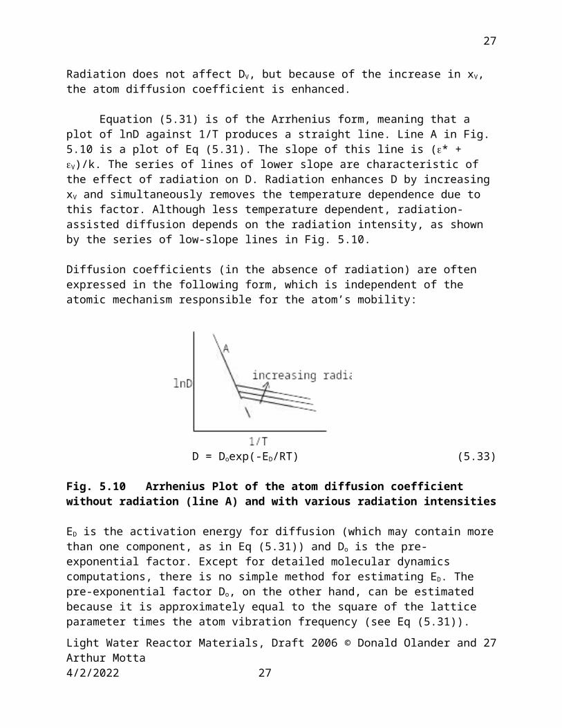
Equation (5.31) is of the Arrhenius form, meaning that a plot of lnD against 1/T produces a straight line. Line A in Fig. 5.10 is a plot of Eq (5.31). The slope of this line is (* + V)/k. The series of lines of lower slope are characteristic of the effect of radiation on D. Radiation enhances D by increasing xV and simultaneously removes the temperature dependence due to this factor. Although less temperature dependent, radiation-assisted diffusion depends on the radiation intensity, as shown by the series of low-slope lines in Fig. 5.10.
Diffusion coefficients (in the absence of radiation) are often expressed in the following form, which is independent of the atomic mechanism responsible for the atom’s mobility:
Light Water Reactor Materials, Draft 2006 © Donald Olander and Arthur Motta 5/16/2023 18
18
18
D = Doexp(-ED/RT) (5.33)
Fig. 5.10 Arrhenius Plot of the atom diffusion coefficient without radiation (line A) and with various radiation intensities
ED is the activation energy for diffusion (which may contain more than one component, as in Eq (5.31)) and Do is the pre-exponential factor. Except for detailed molecular dynamics computations, there is no simple method for estimating ED. The pre-exponential factor Do, on the other hand, can be estimated because it is approximately equal to the square of the lattice parameter times the atom vibration frequency (see Eq (5.31)). With ao 3x10⁻⁸ cm and 1013 s-1, Do is on the order of 0.01 cm2/s, a value that (within an order of magnitude) has been verified experimentally for many systems.
5.5. Types of Diffusion Coefficients
Although the single symbol D has been used to denote the diffusion coefficient, there are several variants of this property. They are classified as follows:
(a) The self diffusion coefficient, D self This property refers to the migration of the atoms of a pure element or the cation or anion of an ionic solid in the absence of a concentration gradient. This is the type of diffusivity deduced from the atomic mechanisms discussed in Sect. 5.4. There is no direct method for measuring the self-diffusion coefficient.
(b) The tracer diffusion coefficient, Dtr
This diffusivity is subject to the same conditions as the self-diffusion coefficient except that some of the atoms are radioactive isotopes of the host element or ion. Measurement of Dtr requires a gradient (and hence a flux) of the tracer but there is no gradient or flux of the combined radioactive and nonradioactive element or ion. The diffusivities of these two forms are equal.
Dself = Dtr (5.34)
Light Water Reactor Materials, Draft 2006 © Donald Olander and Arthur Motta 5/16/2023 19
19
19
(c) The Intrinsic Diffusion coefficient DIn
This quantity refers to the diffusion of a species in a binary solid. Each species possesses an intrinsic diffusion coefficient, designated as and for the components A and B respectively. A and B can refer to the components of a binary metallic alloy (e.g. Fe and Ni) or the cation and anion of an ionic solid (e.g. Na+ and Cl-). Intrinsic diffusivities could also refer, for example, to U4+ and Pu4+ interdiffusing in the mixed oxide (U,Pu)O2. The intrinsic diffusivities of the components of a binary solid are in general not equal. These diffusivities imply concentration gradients of the species A and B, in contrast to the gradient-free self- and tracer diffusion coefficients.
The classic experiment by which the existence of intrinsic diffusivities was first revealed utilized the diffusion couple shown on the right hand side of Fig. 5.2. The two solids are different metals completely miscible in each other. In preparing the couple, the interface is “marked” by placing a series of inert metal wires (e.g., Ta) between the two blocks. The wires are thin enough not to impede interdiffusion of the species on either side of them. During the diffusion anneal, the markers are found to move relative to the stationary ends of the couple. This fact implies that the two species do not migrate at the same rates, or that they have different intrinsic diffusion coefficients. Both species obey Fick’s law with the moving marker interface as the origin of the distance x.
(d) The Mutual Diffusion Coefficient This type of diffusion coefficient is also called the chemical or inter-diffusion coefficient. It is closely related to the marker experiment described in the preceding paragraph. Measurement of the A-B concentration gradient relative to the fixed ends of the diffusion couple (rather than relative to the marker wires) produces . The intrinsic diffusivities and the mutual diffusion coefficient are related by the so-called Darken equation:
(5.35)
A derivation of this equation is given in the book by Shewmon (4).
Relations between the Types of Diffusion Coefficients The connection between the mutual and intrinsic diffusivities on one hand and
the self or tracer diffusivities on the other arises from the following fact: the correct gradient that drives diffusion is that of the chemical potential, not of the concentration (which appears in Fick’s law), or the mole fraction, which is directly related to the concentration. Using Eqs (1.36) and (1.37) of Chap. 1, it can be shown that the relation is:
(5.36)
where A is the activity coefficient of component A in the A-B solution. The crucial part of this expression is the nonideality correction in the parentheses. The self- or tracer Light Water Reactor Materials, Draft 2006 © Donald Olander and Arthur Motta 5/16/2023 20
20
20
diffusion coefficients are applicable to conditions of constant concentration and so do not involve the nonideality effect. Detailed application of this feature (see Ref. 4) leads to the following relation:
(5.37)
The second term in the parentheses is, by the Gibbs-Duhem equation , Eq (1.38), equal to the comparable term for component B. Substitution of Eq (5.37) and its analog for component B into Eq (5.35) yields:
(5.38)
The term in parentheses is unity for either ideal solutions (A = 1) or for dilute solutions (A = constant, by Henry’s law). In principle, the mutual diffusion coefficient could be obtained by measuring the tracer diffusion coefficients of A and B and the nonideality correction. In practice, the mutual diffusion coefficient is measured directly. If the solution is dilute in A, Eq (5.38) reduces to and if it is dilute in B, . For ideal solutions, is the mole-fraction-weighted average of the tracer diffusion coefficients. In practice, in elemental binary solids only the mutual diffusion coefficient is of interest, and it is denoted simply as D, without the tilde. In ionic solids, the two species generally have such different intrinsic diffusivities that separate values for Dcation and Danion are needed.
5.6. Diffusion in Ionic Crystals
Diffusion in ionic crystals differs from that in metals and elements in numerous ways:
1. Ionic solids contain at least two components and the two are oppositely charged2. Cations and anions generally exhibit very large differences in intrinsic diffusivities;
occasionally as large as seven orders of magnitude3. The type of defect that predominates (Schottky or Frenkel) controls the magnitudes
of the diffusivities4. The effect of substitutional doping of ionic solids with cations of different valence
from the host cation has a profound effect on the diffusivities, often of both ions.5. The requirement of local electrical neutrality affects the movement of the ions.6. Interstitial impurity diffusion is not as important in ionic solids as it is in metals and
other elements.
On the other hand, there is considerable commonality between diffusion in metals and in ionic compounds:
Light Water Reactor Materials, Draft 2006 © Donald Olander and Arthur Motta 5/16/2023 21
21
21
1. The diffusion coefficients obey the Einstein equation, Eq(5.28)2. The mechanisms commonly found in metals and elements (vacancy and
interstitial) also predominate in ionic solids3. The various types of diffusion coefficients discussed in the preceding section
(intrinsic, tracer, self, mutual) are also present in ionic solids.4. The relation between point defect properties (concentration and mobility) and the
ion diffusivity is the same for ionic solids as it is for metals and other elements (Eq (5.32a) for the vacancy mechanism). However, motion of the ions is restricted to the sublattice of the same charge. For an ionic solid generically labeled MXn, the tracer diffusion coefficients are:
Vacancy mechanism: (5.39a)
Interstitial mechanism: (5.39b)
In general, the self or tracer diffusion coefficients depend linearly on the concentrations (site fractions) of the point defect responsible for atom motion. The diffusivities of the defects proper, however, are independent of their concentrations.
All four mechanisms are not operative in a particular ionic solid. The mechanism that dominates for the cations may be different from that controlling anion motion.
The NaCl-type Structure with Schottky Defects
The intrinsic diffusion coefficients are the same as the tracer diffusivities because electrical neutrality forbids generation of concentration gradients in which the Na/Cl ion ratio differs from unity (i.e., the thermodynamic factor in Eq (5.37) is unity). In this lattice type, the cation intrinsic diffusivity is substantially larger than the anion diffusivity, or
.
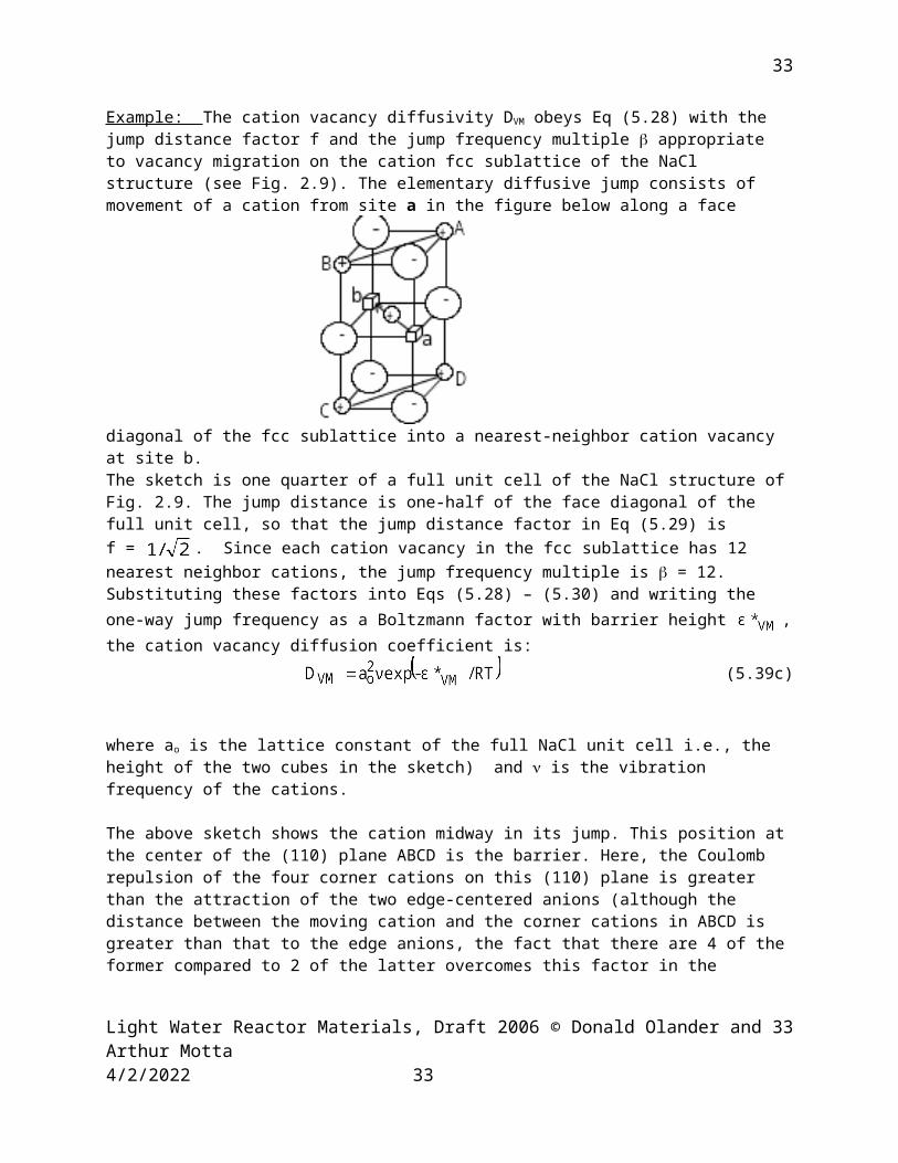
Example: The cation vacancy diffusivity DVM obeys Eq (5.28) with the jump distance factor f and the jump frequency multiple appropriate to vacancy migration on the cation fcc sublattice of the NaCl structure (see Fig. 2.9). The elementary diffusive jump consists of movement of a cation from site a in the figure below along a face diagonal of the fcc sublattice into a nearest-neighbor cation vacancy at site b.
Light Water Reactor Materials, Draft 2006 © Donald Olander and Arthur Motta 5/16/2023 22
22
22
The sketch is one quarter of a full unit cell of the NaCl structure of Fig. 2.9. The jump distance is one-half of the face diagonal of the full unit cell, so that the jump distance factor in Eq (5.29) is f = . Since each cation vacancy in the fcc sublattice has 12 nearest neighbor cations, the jump frequency multiple is = 12. Substituting these factors into Eqs (5.28) – (5.30) and writing the one-way jump frequency as a Boltzmann factor with barrier height , the cation vacancy diffusion coefficient is:
(5.39c)
where ao is the lattice constant of the full NaCl unit cell i.e., the height of the two cubes in the sketch) and is the vibration frequency of the cations.
The above sketch shows the cation midway in its jump. This position at the center of the (110) plane ABCD is the barrier. Here, the Coulomb repulsion of the four corner cations on this (110) plane is greater than the attraction of the two edge-centered anions (although the distance between the moving cation and the corner cations in ABCD is greater than that to the edge anions, the fact that there are 4 of the former compared to 2 of the latter overcomes this factor in the Coulomb potential). This excess Coulomb repulsion midway along the jump is the source of the barrier energy .
The diffusion coefficient of the cations is obtained by multiplying DVM by the vacancy fraction, xVM. For high-purity NaCl, intrinsic point defects dominate and xVM is given by Eq (4.11), or xVM = , where KS is the equilibrium constant for Schottky defects. The activation energy for diffusion is the sum of the migration energy of the cation vacancy, , and one half of the energy of formation of the Schottky defects, ½ S. The energy of formation of Schottky pairs in NaCl is ~ 220 kJ/mole. Neglecting the entropy term in Eq (4.8), at 1000K, KS = 3x10-12 and xVM ~ 2x10⁻⁶.
Ionic solids are rarely so pure that intrinsic point defects control the point defect concentrations. If a divalent impurity cation is present, the cation vacancy fraction in NaCl is given by Eq (4.26):
(3.26)
where xD is the cation site fraction of the divalent dopant. This impurity exerts a significant effect on the point defect concentration for xD as low as 2x10⁻⁶, where the above equation gives xVM = 3x10⁻⁶. For impurity concentrations greater than a few parts per million, Eq (4.26) reduces to the extrinsic limit, xVM ~ xD. Excepting ultra-high-purity material, the cation diffusivity given by the first of Eq (5.39a) in NaCl is entirely controlled, via xVM, by the concentration of divalent impurity ions. Impurity cations of the same charge, such as K+, do not affect xVM and hence do not influence .
Light Water Reactor Materials, Draft 2006 © Donald Olander and Arthur Motta 5/16/2023 23
23
23
5.7. Diffusion in the Fluorite Structure of UO2
Diffusion in uranium dioxide of greater importance and substantially more complicated than in the NaCl example reviewed in the preceding section. First, the diffusivities of the anion (oxygen) and the cation (uranium), although very different in magnitude, are both technologically important. Second, diffusion of impurity species, both ionic and neutral, influence the behavior of nuclear fuel. Third, the multiplicity of uranium oxidation states permits extrinsic point defects to control the diffusivity: U5+ is effectively a dopant on the cation sublattice. Fourth, intrinsic point defects, important around exact stoichiometry, are controlled by both anion Frenkel and Schottky processes. Although the migration of the ions are restricted to their proper sublattices, the point defect equilibrium involving one component can affect the point defect concentration, and hence the diffusivity, on the other sublattice.
Oxygen Diffusion Both the self (tracer) diffusivity and the chemical diffusivity of oxygen in UO2y
have been measured and the thermodynamic factor connecting the two (as in Eq (5.37)) has verified their relationship. The tracer diffusion coefficient is measured using the techniques described in Sect. 5.3 with stable 18O isotope as the diffusing species in place of a radioactive tracer. In considering the U-O system as a binary, the chemical diffusivity effectively reduces to the tracer diffusivity of oxygen because >> (see Eq (5.38) with A = O and B = U). Both types of diffusion coefficients (tracer and chemical) depend on the stoichiometry of the oxide, that is, on the O/U ratio as it varies from < 2, through 2, to >2.
In hyperstoichiometric urania, the excess oxygen (i.e., y in UO2+y) exists as interstitials of the type shown in Fig. 3.6. The oxygen vacancy concentration is small because of the anion Frenkel equilibrium, which dominates in urania:
(5.40)
where R = 8.314 J/mole-K. If the oxygen interstitial concentration is large, the oxygen vacancy concentration is small.
With oxygen interstitials as the dominant defect, diffusion takes place by the interstitial mechanism* ,so the tracer (or self-) diffusion coefficient of oxygen is:
(5.41)
* Acually, the mechanism is called the interstialcy mechanism. Rather than the moving atom jumping from one interstitial site directly to a neighboring interstitial site, as in Fig. 4.5.5, the interstitial pushes an adjacent regular lattice atom into the neighboring interstitial site and the original interstitial replaces the departed lattice ion (see Ref. 4, p. 59)Light Water Reactor Materials, Draft 2006 © Donald Olander and Arthur Motta 5/16/2023 24
24
24
Where DIO is the diffusion coefficient of oxygen interstitials per se and xIO is the site fraction of oxygen interstitials. The latter is given in terms of the stoichiometry excess parameter y by Eqs (3.35) and (3.36a):
(5.42)
If the temperature is sufficiently low and y sufficiently large, 24KFO/y2 << 1 and Eq (5.42) reduces to:
xIO = y/3 (5.42a)
The measured values of in UO2+y together with the approximation of xIO by Eq (5.42a) permits the diffusivity of oxygen interstitials to be determined. The result is (5):
(5.43)
where = 100 kJ/mole is the energy barrier for the movement of interstitial oxygen ions. Without making the approximation of Eq (5.42a), substitution of Eqs (5.42) and (5.43) into Eq (5.41) gives the tracer diffusivity when both the extrinsic interstitials (due to y in Eq (5.42)) and the intrinsic interstitials (represented by KFO in Eq (5.42) are of comparable importance. In the limit as y = 0, Eq(5.42) reduces to:
(5.42b)
Inserting Eq (5.40) into (5.42b) and the result, along with Eq (5.43), into Eq (5.41) gives the tracer diffusivity of oxygen in stoichiometric UO2:
cm2/s (5.44)
Equation (5.44) agrees with the formula given by Matzke (6), which originated from the work of Ref (7). The activation energy is in kJ/mole.
Similar data and analyses are available for oxygen tracer self diffusion in hypostoichiometric urania, UO2-y (see refs 5, 8 and 9), but because of the limited technological interest of this material in light water reactor technology, this topic is not considered here in detail. The most important feature of oxygen diffusion in this material is that it occurs by the vacancy mechanism, anion vacancies being the dominant point defect in a deficit of oxygen.
The tracer diffusion coefficient appeals to theorists because of its close connection to atomistic models and avoidance of the difficulties introduced in the presence of a concentration gradient. However, the chemical diffusivity of oxygen, , has the important practical implications;
Light Water Reactor Materials, Draft 2006 © Donald Olander and Arthur Motta 5/16/2023 25
25
25
in fast oxide reactors, this quantity controls the radial redistribution of oxygen in the fuel;
the kinetics of oxidation of UO2 to UO2+y or reduction to UO2-y are determined by this property;
the oxide scale that forms on the Zircaloy cladding exposed to water forms at a rate dependent on in ZrO2.
The chemical diffusion coefficient of oxygen in urania can be measured by one of several relatively simple experiments. The principle tool used for this purpose is measurement of the weight change of a specimen of the oxide suspended in the hot zone of a furnace from a microbalance through which flows a gas of known oxygen pressure. This oxygen pressure and the temperature fix the O/U ratio at the surface of the urania specimen. Oxygen diffuses between this surface and the interior in a direction dictated by the thermodynamics of UO2y and at a rate determined by .
The chemical diffusion coefficient in UO2+y describes the flux of oxygen in an O/U gradient. Since the uranium sublattice is structurally practically perfect, the gradient is due to a change in the concentration of oxygen interstitials. The U5+/U4+ ratio varies in order to maintain electrical neutrality in this gradient of oxygen.
The tracer diffusivity and the chemical diffusivity are related by a variant of Darken’s formula, Eq (5.38). Since >> , and the activity coefficient of oxygen can be converted to the activity by the relation aO =xOO, the relation is:
(5.45)
In UO2+y, the mole fractions are related to the stoichiometry excess parameter y by:
and (5.46)
The activity of oxygen in the solid is related to the pressure of O2 in the gas by the equilibrium of the reaction:
O2(g) = 2O(interstitial in solid)
The condition of equilibrium is written in terms of the chemical potentials:
Taking pure oxygen gas at 1 atm as the standard state for both chemical potentials, Eqs (1.35) and (1.44) of Chap. 1 transform the above equation to:
(5.47)
Light Water Reactor Materials, Draft 2006 © Donald Olander and Arthur Motta 5/16/2023 26
26
26
Substituting Eqs (5.46) and (5.47) into Eq (5.45) yields:
(5.48)
The thermodynamic factor is a function of T and y. For practical purposes, it is roughly independent of both. When the approximation of Eq (5.42a) applies (i.e., when y > 0.001), the tracer diffusion coefficient becomes:
(5.49)
where DIO is given by Eq (5.43). Substitution of Eq (5.49) into Eq (5.48) shows that is practically independent of y, or of the O/U ratio.
Many measurements of are available in the literature. A typical experimental result is (10):
cm2/s (5.50)
The activation energy is in J/mole. The experimental migration energy from Eq (5.50) is of the same order of magnitude as the value deduced from the entirely different measurements of the tracer diffusion coefficient given by Eq (5.43). A more detailed account of the relationship between and can be found in Refs 5 and 11.
The chemical diffusion coefficient from Eq (5.50) is very high. At T ~ 1000oC, is comparable in magnitude to the diffusivity of solutes in liquids at room temperatures, that is, about 10-5 cm2/s.
Uranium Diffusion
There are three types of motion that uranium cations undergo in oxide nuclear fuels. However, they are characterized by the two usual types of diffusion coefficients: self (or tracer) diffusion and chemical (or inter) diffusion.
Uranium Self-Diffusion in UO2
Self diffusion describes the random walk of uranium ions on the cation sublattice in the absence of a concentration gradient. It can be measured by one of the techniques shown in Fig. 5.2, where the diffusing species is a radioactive uranium isotope, say 233U.
Light Water Reactor Materials, Draft 2006 © Donald Olander and Arthur Motta 5/16/2023 27
27
27
Uranium self (or tracer) diffusion in UO2 occurs by the vacancy mechanism on the cation sublattice. The diffusion coefficient is given by the first of Eqs (5.39a):
(5.51)
where DVU is the diffusion coefficient of cation vacancies and xVU is the concentration (site fraction) of uranium ion vacancies. The former is calculated from the Einstein relation (Eq(5.28)) by specifying the jump distance and jump frequency for this mechanism* . However, to a first approximation, there are no thermodynamically-generated cation vacancies in UO2. The reason is that the major point defects are anion Frenkel pairs. The cation vacancies needed for uranium diffusion (even in hyperstoichiometric urania) are generated by the Schottky process,
null = VU + 2VO (5.52)
whose equilibrium constant , KS, is much smaller than the anion Frenkel equilibrium constant KFO (see Eq (3.28) et seq.). The Schottky equilibrium is:
(5.53)
The site fractions xVU and xVO are referenced to the numbers of cation and anion lattice sites, respectively. KS is given by:
(5.54)
where S = 544 kJ/mole is the energy of formation of the Schottky defect in UO2.
Because the concentration of Schottky defects in UO2 is small compared to the point defect concentration produced on the anion sublattice by the Frenkel process, the analysis of the latter is not significantly affected by the Schottky equilibrium. Specifically, the oxygen vacancy fraction is expressed by Eq (3.36b).
Example: Compare the anion and cation vacancy fractions in stoichiometric UO2 at 2000 K.
For y = 0, Eq (3.35) reduces to g(0) = , and from Eq (3.36b),
Using this result in Eq (5.53)
At 2000 K, KFO = 3.4x10⁻⁵ and KS = 8x10-15. Using these values in the above equations gives* These factors are identical to those determined for the cation vacancies in the NaCl structure treated in the example in the beginning of this section.Light Water Reactor Materials, Draft 2006 © Donald Olander and Arthur Motta 5/16/2023 28
28
28
xVO = 7x10⁻³ and xVU = 1.5x10⁻¹⁰.
With DVU given by Eq (5.39c) and the above expression for xVU, Eq (5.51) gives the tracer diffusivity of U in stoichiometric UO2:
(5.55a)
Expressing KS and KFO in terms of their entropies and energies of formation changes the above equation to:
(5.55b)
In numerical terms, the above formula is (12):
cm2/s (5.55c)
The units of the activation energy are kJ/mole. The great difference between the tracer diffusivities of oxygen and uranium in stoichiometric UO2 can be attributed to the difference in the activation energies in Eqs (5.44) and (5.55c). The high activation energy in the latter equation is due to the large energy of formation of Schottky defects in UO2 .
For application of the point-defect model to hyperstoichiometric urania (UO2+y), the starting point for determination of the tracer diffusivity of uranium is the oxygen vacancy fraction of Eq (3.36b) with the function g(y) given by Eq (3.35). Combining these two equations yields:
` (5.56)
This equation is substituted into the Schottky equilibrium of Eq (5.53) for determination of xVU which, along with Eq (5.39c), gives the uranium self diffusion coefficient.
This process can be simplified if the term 24KFO/y2 in Eq (5.56) is << 1. In this limit, a one-term Taylor series expansion of the square root term gives xVO = 3KFO/y. When inserted into Eq (5.53), this approximation results in:
(5.57)
Light Water Reactor Materials, Draft 2006 © Donald Olander and Arthur Motta 5/16/2023 29
29
29
Care needs to be exercised in using this approximation. For example, at 2000K, where KFO = 3.4x10⁻⁵, at y = 0.01, the limiting form of xVO is twice a large as the value obtained from Eq (5.56). For y = 0.05, the error decreases to 7%.
Substituting Eqs (5.57) and (5.39c) into the first of Eqs (5.39a) and expressing KS
and KFO in terms of the entropies and energies of point defect formation yields:
(5.58)
where KFO is given by Eq (5.40), S = 544 kJ/mole, and kJ/mole (Ref 12).
Experimental data from numerous sources are summarized on Fig. 5.11.
Fig. 5.11 Effect of Stoichiometry on the Self-Diffusion Coefficient of Uranium in UO2+x at 1500oC (after Ref. 13)
The two curves in the plot are visual fits to the data. The lowest datum (open circle) is a result for nominally stoichiometric UO2. The value computed from Eq (5.55c) is 10-16 cm2/s. The O/U interval indicated by y is the region where changes by several orders of magnitude.
The value of (UO2.1 ) calculated from Eq (5.58) at 1500oC is 8x10-17 cm2/s, which is approximately three orders of magnitude lower than the data in Fig. 5.11 at the same O/U ratio. This suggests a massive failure of the point defect model upon which Eq (5.58) is based. However, the stoichiometry dependence of predicted by Eq (5.58) is consistent with the data. For example, the ratio (2.10)/ (2.05) from Fig. 5.11 is ~ 4, which corresponds exactly with the y2 dependence in Eq (5.58). The most
Light Water Reactor Materials, Draft 2006 © Donald Olander and Arthur Motta 5/16/2023 30
30
30
likely source of the discrepancy between the measured and predicted values of lies in the uncertainties in the three components of the activation in Eq (5.58) and in the unknown entropy of formation of Schottky defects in UO2, which has arbitrarily been set equal to zero.
The type of diffusive motion in UO2 that is directly dependent on the uranium tracer diffusion coefficient is called net matter transport . It occurs when UO2 molecules move with respect to a fixed point within the fuel. A good example of this type of transport occurs during sintering. In this process, the pores inside the fuel pellet shrink as the oxide densifies. Pore shrinkage can be visualized either as emission of uranium vacancies from the pore or as accumulation of uranium atoms on the surface of the pore. In either case, UO2 is transported relative to the center of the pore, which is regarded as a fixed origin. The growth of fission gas bubbles during irradiation is in effect loss of UO2 molecules from the bubble surface. This process is the inverse of pore shrinkage.
Another example of net matter transport is creep of UO2 in a uniaxial tensile stress. The mechanism of this process involves movement of UO2 from grain boundaries oriented parallel to the stress direction to grain boundaries perpendicular to the stress direction. The fixed origin for gauging this transport rate is the center of the deforming grain. The temperature dependence of the creep rate in UO2 closely parallels the temperature variation of shown in Fig. 5.11.
The kinetics of these net matter transport processes are controlled by the uranium self diffusion coefficient. The differences between the usual self-diffusion experiment and the net matter transport process are twofold. First, the direction of molecular motion is not strictly random, as in the former case, but is directed towards a particular object in the microstructure (i.e., the pore or bubble surface or a properly-oriented grain boundary). Second, both uranium and oxygen must move as a unit in a ratio equal to the O/U ratio of the fuel. The uranium ion, being by far much less mobile than the oxygen ion, controls the rate of the net matter transport process. In effect, O2- ions simply tag along with the uranium ions in order to preserve electrical neutrality.
Interdiffusion in Mixed Ionic Solids with the Fluorite Structure
Cooper and Heasley have developed an extension of Darken’s equation (Eq(15.35)) for the chemical (inter-) diffusion coefficient in a solid solution with cations M and N and a common anion X (14). Their expression depends on the valences v i of the three ions, their tracer diffusion coefficients, , and the cation fractions of the two compounds comprising the solid solution, xM and xN (note that xM + xN = 1). In the fluorite structure, the anion diffusivity is much larger than that of the cations, and the interdiffusion coefficient is given by:
Light Water Reactor Materials, Draft 2006 © Donald Olander and Arthur Motta 5/16/2023 31
31
31
(5.59)
Note that the thermodynamic factor in parentheses could equally well have been expressed in terms of the compound designated by N.
Even in the case that cations M and N have the same valence (as in the solution CaF2/SrF2), the interdiffusion coefficient is composition dependent at a fixed temperature because the two tracer diffusion coefficients are different (15). Moreover, when written in the usual Arrhenius form:
(5.60)
The activation energy * depends on composition.
On the other hand, the interdiffusion coefficient in the mixed oxide (ZrzHf1-z)O2 (which has been stabilized in the fluorite crystal structure by addition of CaO) is independent of composition (i.e., of z) and follows Eq (5.60) with a constant activation energy (16). This simple behavior is due to the strong chemical similarity between zirconium and hafnium, which results in and Zr = Hf (ideal solution behavior).
When CaF2 is doped with trivalent yttrium in the form of YF3, extrinsic point defects form to satisfy electrical neutrality requirements, a complication absent when the two cations are of the same valence. There are two possibilities. By analogy to the cation vacancies formed when a divalent cation is added to NaCl (see Eq (3.21) et seq), two Y3+ added to CaF2 could be accompanied by the formation of one vacancy on the Ca2+ sublattice. Alternatively, the extra positive charge due to an added Y3+ could be compensated electrically by an F- interstitial. The latter process actually occurs, with no direct (extrinsic) effect on the cation vacancy concentration. Since self diffusion of Y3+
and Ca2+ on the cation sublattice takes place by a vacancy mechanism, the doping effect on diffusion is manifest by point defect equilibria: the increase in the F- interstitial concentration (xIF) with YF3 doping decreases the F- vacancy concentration (xVF) by the anion Frenkel equilibrium, KFF = xVFxIF; by the Schottky equilibrium, KS = xVM , the cation vacancy concentration (xVM) increases with yttrium doping. This roundabout mechanism of accelerating cation self diffusion is equivalent to that active in hyperstoichiometric urania, wherein U5+ created from some of the normal U4+ by the prevailing oxygen pressure is the analog of the Y3+ expressly added to CaF2.
The cation vacancy concentration affects the self (or tracer) diffusivities by the formulas: and , where DVCa
and DVY are the diffusion coefficients of cation vacancies that exchange with lattice Ca2+ and lattice Y3+, respectively. Hence, as xVM increases with YF3 addition, so do the self diffusion coefficients of the two cations, and via Eq (5.59), the interdiffusion coefficient as well (17). The effect is much more pronounced than in the CaF2/SrF2 binary, where both
Light Water Reactor Materials, Draft 2006 © Donald Olander and Arthur Motta 5/16/2023 32
32
32
cations have the same valence and the cation vacancy amplification mechanism described above is absent.
There are numerous technologically important examples in which uranium ions move relative to a substitutional impurity cation in a concentration gradient of the two. Such interdiffusion occurs, for example, during homogenization of mixed oxide fuel (MOX) during which small particles of initially pure PuO2 mix by diffusion with the UO2 matrix in which they are embedded during fabrication. In another example, during a severe accident at high fuel temperature, a fuel-soluble fission product (e.g., La) may have a higher vapor pressure (as an oxide) than UO2, and evaporate from a free surface at a higher rate than the latter. This depletes the surface of the fission product and produces a near-surface concentration gradient involving the fission product cation and the uranium cation. Transport in such a gradient is governed by the interdiffusion coefficient of the two cation species.
The mixed oxide (U1-zPuz)O2y differs from the previous examples of mixed ionic solids in one important aspect. Instead of cations of fixed valences, U and Pu in the oxide exhibit valences that vary with the oxygen pressure of the ambient gas. Plutonium can be either tri- or tetravalent; uranium valences vary from 4+ to 6+. The possibility of Pu3+ means that the mixed oxide can be hypostoichiometric, or the O/M ratio (M = U + Pu) can be less than two. In fact, O/M 1.98 is the desired fuel stoichiometry in fast reactors because the oxygen deficit makes the fuel less corrosive towards the stainless steel cladding. The sign in the mixed oxide formula serves of keep the stoichiometry parameter y positive. Hypostoichiometric oxide is denoted by (U1-zPuz)O2-y and O/M < 2 while the hyperstoichiometric oxide is written as (U1-zPuz)O2+y and O/M > 2.
The oxidizing power of the environment is fixed by the pressure of O2, or, alternatively, the oxygen potential:
(5.61)
The units of the of are kJ/mole, or kcal/mole. The oxygen potential of a gas can be established in numerous ways; a common method is a mixture of CO2 and CO with a known CO2/CO ratio. Application of this method is given in the example at the end of Sect. 1.8 of Chap. 1.
The thermochemistry of mixed U-Pu oxides is treated in Chap. X. For the present purpose, it suffices to note that the temperature and the oxygen potential determine the valence of the actinide cations in the solid. At low oxygen potentials, for example, all uranium is in the 4+ valence state and the plutonium valence (vPu) is between 3+ and 4+. The relation between vPu , the plutonium fraction z and the stoichiometry deficit y is obtained from the condition of electrical neutrality:
vPu z + 4(1-z) = 2(2-y) or y = ½z(4 – vPu) (5.62a)
Light Water Reactor Materials, Draft 2006 © Donald Olander and Arthur Motta 5/16/2023 33
33
33
The thermochemistry of the mixed oxide gives the function vPu(T, ), the second of these variables being fixed by the composition of the gas phase contacting the solid. With Eq (5.62a), the stoichiometry deficit y is dependent on the same two variables and in addition, on the Pu fraction z.
At high oxygen potentials all Pu is tetravalent and the uranium valence is somewhere between 4+ and 6+. The electrical neutrality condition in this case is
4z + vU(1-z) = 2(2+y) or y = ½(1-z)(vU – 4) (5.62b)
By the thermochemistry of the mixed oxide, the uranium valence vU depends on T and . According to Eq (5.62b), the stoichiometry excess y is a function of T,
and z.
Except in a reactor fuel rod, uranium-plutonium interdiffusion usually takes place at uniform temperature and oxygen potential. In such a process, the Pu fraction (z) varies along the diffusion path. Consequently, the O/M ratio, 2 y, is also a function of position.
The tracer diffusion coefficients and are functions of all three variables (T, , and z). In Eq (5.59) with M = U and N = Pu, xN = z and xM = 1-z, the interdiffusion coefficient is also a function of the same three variables. The available data are not sufficient to relate the tracer diffusivities and the interdiffusion coefficient via Eq (5.59). The left hand panel of Fig. 5.12 shows the dependence of on oxygen potential and Pu concentration at T = 1500oC. These data show a rapid increase in with increasing oxygen potential and increasing Pu fraction. Strictly speaking, the complex dependence of on three variables precludes representing this property an a simple Arrhenius plot. However, to compare the many attempts to measure that have appeared in the literature, such a plot is shown in the right hand side of Fig. 5.12.
Light Water Reactor Materials, Draft 2006 © Donald Olander and Arthur Motta 5/16/2023 34
34
34

Fig. 5.12 The interdiffusion coefficient for the UO2 – PuO2 system. Left: as a function of Pu content with the oxygen potential as a parameter (1500oC); right: temperature dependence taken from various sources. The data from the left-hand plot at z = 0.15 are shown as solid circles connected by the bracket. (after Ref. 18)
At oxygen potentials that render the oxide hyperstoichiometric or even slightly hypostoichiometric, diffusion takes place by the cation vacancy mechanism characteristic of other mixed ionic solids of the fluorite structure (see preceding examples). This mechanism (principal anion Frenkel, minor Schottky defect equilibria)is consistent with the strong effect of the oxygen potential seen in Fig. 5.12. In definitely hypostoichiometric oxide, the mechanism appears to involve metal interstitials. At 1500oC, the switch in the mechanisms occurs at O/M = 1.98 (18).
5.8. Thermal Diffusion
Thermal diffusion refers to the transport of atoms driven by a temperature gradient. Unlike ordinary diffusion in a concentration gradient, thermal diffusion is not a random-walk process; the affected atoms flow along the temperature gradient, either up or down. Thermal diffusion affects impurity atoms in a host crystal, the important example being hydrogen in Zircaloy (treated in Chap. XX). In the steep temperature gradient of a fast reactor fuel pin, oxygen in (U,Pu)O2y migrates radially, causing an O/M variation from the center to the fuel pellet surface. Independently, plutonium moves in the temperature gradient, resulting in unmixing of the actinide composition of the fuel.
Light Water Reactor Materials, Draft 2006 © Donald Olander and Arthur Motta 5/16/2023 35
35
35
Thermal diffusion is determined by a property of the species in the solid called the heat of transport, which is denoted by Q* in units of kJ/mole. The thermal diffusion effect is accounted for as an additive term to the concentration gradient in the following form:
(5.63)
A simple method for measuring Q* is available: a rod of the host solid initially containing a uniform concentration of an impurity species is heated to temperature TH at one end and maintained at a lower temperature TC at the other end. The impurity species cannot leave the rod at either end, so it merely redistributes in the temperature gradient. After a time sufficiently long for steady state to be achieved, the flux is everywhere zero. Setting J = 0 in Eq (5.63) and eliminating dx results in:
integrating yields:
(5.64)
The rod is cut into slices and the concentration of the impurity species measured as a function of the distance x. Knowing the temperature distribution T(x) (it is usually linear) provides data in the form of c vs T. Plotting lnc Vs 1/T yields a straight line whose slope is Q*/R. The slope, and hence Q*, can be either positive or negative.
Explanation of the sign of Q* is given in Ref. 5. In brief, the activation energy for the diffusive jump that appears as the single property * for the isothermal case needs to be refined as follows when the temperature is nonuniform:
* = o + f
The first component on the right (o ) represents the energy given to the impurity atom in its initial equilibrium site by the thermal vibrations of the neighboring host atoms. The second component (f) is the energy required to configure the final equilibrium site for accepting the jumping impurity atom. By considering the effect of a temperature difference on the jump frequencies in the initial and final sites, the heat of transport is:
Q* = o - f (5.65)
Depending on the magnitudes of o and f, Q* can be positive or negative. In either case, the absolute magnitude must be less than *.
Light Water Reactor Materials, Draft 2006 © Donald Olander and Arthur Motta 5/16/2023 36
36
36
Appendix 5A Dimensionless Variables and the Similarity Transformation Solution to Eq s (5.4) – (5.7)
The objective is to convert the Eq (5.4) into an ordinary differential equation which can be solved analytically. To this end, the following dimensionless variables are introduced:
= c/c0 (source) (5A.1a)
= c/(c0/2) (couple) (5A.1b)
xDt2
(5A.2)
Equation (5A.2) is called the similarity transformation. The new variable is a function of both x and t. In terms of this variable, the partial derivatives in Eq (5.4) are:
ct t
c xD t
ctc
2
12 23 2/
cx x
cDt
c 12
2
2
2
21
214
cx x
cx x Dt
cDt
c
Using these transformations in Eq (5.4)) converts the partial differential equation to an ordinary differential equation:
dd
dd
2
2 2 0
(5A.3)
The initial and boundary conditions reduce to:
= 1 at (Eqs (5.6a) and (5.6b)) (5A.4)
0 at (Eqs (5.5) and (5.7)) (5A.5)
It is necessary for this method to work that the initial condition and two boundary conditions of the original set reduce to two boundary conditions in the variable .
Solution of Eq (5A.3) subject to Eqs (5A.4) and (5A.5) is accomplished by introducing a new dependent variable U = d/d, which reduces Eq (5A.3) to a first order differential equation:
dU/d + 2U = 0
Light Water Reactor Materials, Draft 2006 © Donald Olander and Arthur Motta 5/16/2023 37
37
37
The first integral of this equation is:
U dd
A
exp( )2
Integrating again:
A d Bexp( )2
0
Applying the boundary conditions given by Eqs (5A.4) and (5A.5) yields the integration constants:
B=1 and A d
exp( )
2
0
1 2
The dimensionless form of the solution is:
(5A.6)
which, when returned to dimensional forms using Eqs (5A.1) and (5A.2), yields Eqs (5.8a) and (5.8b).
Light Water Reactor Materials, Draft 2006 © Donald Olander and Arthur Motta 5/16/2023 38
38
38
Appendix 5B Laplace Transform Solution to Eqs (5.16) – (5.18)
The first steps are to introduce dimensionless variables and a new independent variable that converts the diffusion equation from spherical to slab geometry:
= r/a; = Dt/a2 u = (r/a)c/co = c/co (5B.1)
Substituting Ea(5B.1) into Eqs (5.16) - (5.18) yields:
u u
2
2 (5B.2)
u(,0) = (5B.3)
u(0,) = 0; u(1,) = 0 (5B.4)
Taking the Laplace transform of Eq (5B.2) using Eq (5B.3)*;
d ud
pu2
2
~~
(5B.5)
where p is the transform variable and . The transformed boundary conditions of Eq (5B.4)) become:
~( ) ~( )u u0 1 0 (5B.6)
The solution of the transformed equation is:
(5B.8)
Before inverting the solution, the average concentration is first obtained:
(5B.9)
Taking the Laplace transform of (5B.9) and using (5B.8) yields:
(5B.10)
* The Laplace transform of the time derivative of a function is the transform variable times the transform of the function minus the initial spatial distributionLight Water Reactor Materials, Draft 2006 © Donald Olander and Arthur Motta 5/16/2023 39
39
39
Short times are equivalent to large values of p, so the terms with e p 2 can be neglected in Eq (5B.10), giving:
This transform of the average concentration can be inverted from the table of inverse Laplace transforms to yield the result:
(5B.11)
from which Eq (5.19) of the text is obtained.
Light Water Reactor Materials, Draft 2006 © Donald Olander and Arthur Motta 5/16/2023 40
40
40
Problems
5.1 Show that J of Eq (5.19) is proportional to 1 / t and Q of Eqs (5.18) and (5.20) is proportional to t . Pertinent properties of the error function and the complimentary error function are given below.
erf x e dyyx( )
2 2
0 , erfc x erf x( ) ( ) 1
erf ( )0 0 , erf ( ) 1
erf x x( ) 2 for x << 1, erf x e
x
x
( )
1 22
for x >> 1
ddxerf x e x( ) 2 2
, ddx
erf x x e x2
2
4 2
( )
erfc y dy x erfc x ex x( ) ( ) ( )0
1 12
erfc y dy( )0
1
5.2 In the couple method of measuring solid-state diffusivities, the couple is raised to the desired temperature and held for a fixed length of time. At the end of the experiment, the concentration profile is determined by sectioning or grinding off very thin layers (~1m) of the block and measuring their compositions. The diffusion coefficient is determined by fitting the data to Eq (5.17b).
(a) If the minimum penetration distance required for reliable measurement of the concentration profile is 2 m and the maximum time an experiment can be conducted is 1 year, what is the smallest value of D that can be accurately determined?
(b) If the solute diffuses by an interstitial mechanism in the bcc lattice of the matrix, what is the lowest temperature at which measurements can be made? The activation energy for diffusion is 250 kJ/mole. Make reasonable estimates of any other parameters needed.
5.3 The first wall of a fusion reactor is designed to prevent loss of tritium bred in the blanked fluid circulating inside. The diffusion coefficient of tritium in the metal first wall material is D and the wall thickness is L. At startup, the inner surface of the first wall is exposed to tritium from the plasma which produces a concentration C1 at the metal surface. The opposite face of the first wall is exposed to a circulating coolant fluid that immediately removes any tritium reaching this surface.Light Water Reactor Materials, Draft 2006 © Donald Olander and Arthur Motta 5/16/2023 41
41
41
(a) Write the diffusion equation for tritium transport in the wall and the appropriate initial and boundary conditions.
(b) Make the equations of part (a) dimensionless by choosing appropriate dimensionless variables for time, position in the wall, and tritium concentration.
(c) Without solving the diffusion equation, estimate the time required for significant tritium penetration of the first wall. Assume D = 10-8 cm2/s and L = 0.3 cm. For “significant penetration”, use the following: Assume that the wall were infinite in extent; estimate the time for the concentration at x = L in this infinite solid to reach 2% of the surface concentration.
5.4 Given that you are able to perform a diffusion experiment during a period of 30 days and that you are able to analyze a diffusion layer with thickness of order of 10 -3cm, what is a rough estimate of the smallest diffusion coefficient that could be studied? If the sample is Cu, what is the lowest temperature at which the experiment could be made? If the temperature is incresed to 950 C, how does this afect the time needed to achieve the same result? (Given that for Cu,
)
5.5 Using the Einstein relation, what are the following diffusion coefficients:(a) Vacancy diffusion coefficient by the vacancy mechanism in the elemental bcc
structure. Sketch the potential energy experienced by the moving atom as it moves along its path during the diffusive jump.
(b) Atom self diffusion by the vacancy mechanism in the simple cubic lattice.
5.6 The diffusion of element A into element B is described by the following error function solution
0
0.2
0.4
0.6
0.8
1
1.2
0 0.5 1 1.5 2 2.5
X=x/2sqrt(Dt)
erf(X)
erfc(X)
Light Water Reactor Materials, Draft 2006 © Donald Olander and Arthur Motta 5/16/2023 42
42
42
At the temperature the experiment is conducted the diffusion coefficient of A into B is equal to 10-11 cm2/s.
If Co=1 (such as would occur when there is an inexhaustible supply of A at x=0), answer the following questions:
a) After 2 days of running the experiment, at what distances into the sample would the concentrations be equal to 0.5 and to 0.1?b) For a distance of 1 cm, at what time would you expect to see a concentration of 0.1?c) How would the answers to the above questions change is the temperature is increased twofold? Assume the activation energy for migration of A into B is 1 eV, and that all other terms of Einstein’s diffusion coefficient formula are independent of temperature.
5.7 In Problem 5.3, instead of maintaining zero tritium concentration at the surface, the tritium flux from the wall into the coolant is proportional to the concentration at the outer surface of the wall. The constant of proportionality is kg (units of cm/s), the boundary layer mass transfer coefficient. The sketch below shows the two tritium concentration profiles. The lower line represents the results of problem 5.3.
(a) What is the boundary condition for the tritium diffusion equation at the wall-coolant interface?
(b) What is the equation giving the steady-state permeation rate of tritium through the wall?
(c) Under what conditions is the permeation rate independent of wall thickness?
5.8In the surface-source technique for measuring solid-state diffusivities, a thin layer
of pure solid A of thickness h is deposited on a semi-infinite block of solid B. The solids A and B are immiscible in each other, but at the interface, the solubility of A in B is Co. The solubility of B in A is zero. The mathematical solution to the diffusion equation given by Eq(4.17a) is valid up to the time t* at which the layer of A has completely dissolved in the matrix B
Assuming that the density and molecular weight of A are known, what is t*?
Light Water Reactor Materials, Draft 2006 © Donald Olander and Arthur Motta 5/16/2023 43
43
43
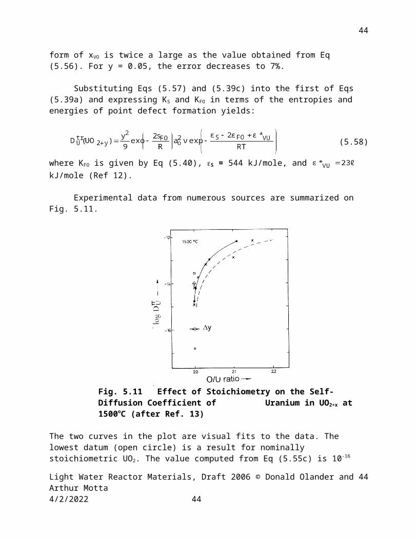
x
solid B
layer of solid A
h
Initial state
final distributionof A in B
x
5.9 A 1 mm thick slab of metal is suddenly exposed to a gas which has a solubility of 1 mole percent in the solid. This concentration is maintained at the slab surface throughout the diffusion process. How long is required for the midplane of the slab to reach a gas concentration of 0.2 mole percent? The diffusion coefficient of the gas in the metal is 2x10⁻⁷ cm2/s.
5.10. A steel component is exposed to a carburizing gas at high temperature to induce the formation of a carbon-rich layer at the metal surface by inward diffusion of carbon atoms. The desired layer measures 0.3mm and the diffusion coefficient of C into fcc Fe at 1000 C is 4 x 10-11 m2s-1. The surface concentration of carbon is 0.5.
a) Use the Einstein formula to find the activation energy. Assume Hz and a jump distance of 2.04 x 10⁻¹⁰ m.
b) Use the error function solution for the concentration profile established in a diffusion couple to derive the annealing time necessary to obtain a 1 at % concentration of C over the desired thickness.
Light Water Reactor Materials, Draft 2006 © Donald Olander and Arthur Motta 5/16/2023 44
44
44
References
1. Carslaw and Jaeger, Conduction of Heat in Solids
2. J. C. Crank, The Mathematics of Diffusion
3. D. R. Olander, Fundamental Aspects of Nuclear Reactor Fuel Elements, National technical Information Service, TID-26711-P1 (1976
4. P. Shewmon, Diffusion in Solids, 2nd Ed., The Minerals, Metals & Materials Society (1989)
5. W. Breitung, Oxygen Self- and Chemical Diffusion Coefficients in UO2x, J. Nucl. Mater. 74 (1978) 10
6. Hj. Matzke, Atomic Mechanisms of Mass Transport in Ceramic Nuclear Fuel Materials, J. Chem. Soc. Faraday Trans. 86 (1990)
7. J. F. Marin and P. Contamin, J. Nucl. Mater., 30 (1969) 16
8. K. Ando and Y. Oishi, J. Nucl. Sci. & Technol. 20 (1983) 973
9. G. Murch, Diffusion and Defect Data, 32 (1983) 4
10. K. Lay, Oxygen Chemical Diffusion Coefficient of Uranium Dioxide, J. Amer. Ceramic Soc. 53 (1970) 369
11. Hj. Matzke, Diffusion in Ceramic Oxide Systems, Adv. in Ceramics 17 (1986) 1
12.Hj. Matzke, Diffusion Processes in Nuclear Fuels, J. of the Less-Common Metals 121 (1986) 537
13. Hj. Matzke, J. Nucl. Mater. 30 (1969) 26
14.A. R. Cooper and J. H. Heasley, J., Amer. Ceramic Soc. 49 (1966) 280
15. R. Scheidecker and M. F. Bernard, J., Amer. Ceramic Soc. 56 (1973) 204
16. Y. Oishi, Y. Sakka and K. Ando, J. Nucl. Mater. 96 (1981) 23
17. R. G. Visser, W. F. Schiavi and M. F. Bernard, J., Amer. Ceramic Soc. 58 (1975) 438
18.D. Glasser-Leme and Hj. Matzke, J. Nucl. Mater., 106 (1982) 211
19. Y. Oishi and H. Ichimura, J. Chem. Phys. 71 (1979) 5134
Light Water Reactor Materials, Draft 2006 © Donald Olander and Arthur Motta 5/16/2023 45
45
45
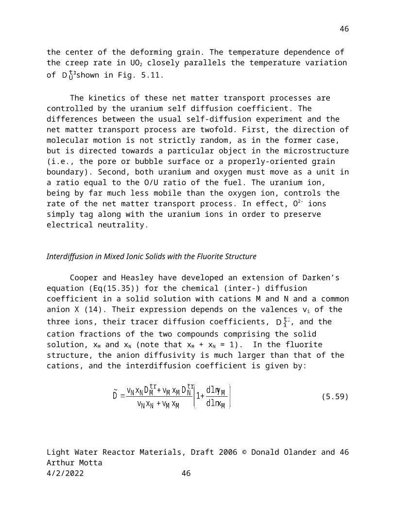
Light Water Reactor Materials, Draft 2006 © Donald Olander and Arthur Motta 5/16/2023 46
46
46