Master’s Thesis in Environmental Science EnvEuro – European Master in Environmental Science

Examensarbeten, Institutionen för mark och miljö, SLU Uppsala 2013 2013:23

3D-printing of undisturbed soil imaged by X-ray Matthias Bacher

SLU, Swedish University of Agricultural Sciences Faculty of Natural Resources and Agricultural Sciences Department of Soil and Environment Matthias Bacher 3D-printing of undisturbed soil imaged by X-ray Supervisor: John Koestel, Department of Soil and Environment, SLU Assistant supervisor: Andreas Schwen, University of Natural Resources and Life Sciences, Vienna, Institute of Hydraulics and Rural Water Management Examiner: Mats Larsbo, Department of Soil and Environment, SLU EX0431, Independent Project in Environmental Science – Master´s thesis, 30 credits, Advanced level, A2E EnvEuro – European Master in Environmental Science, 120 credits Series title: Examensarbeten, Institutionen för mark och miljö, SLU 2013:23 Uppsala 2013 Keywords: soil, macropores, 3D-printing, X-ray Online publication: http://stud.epsilon.slu.se Cover: Soil macropore 3D-printed in different materials, 2013, photo by author

Abstract

An artificial soil pore network can help to analyse preferential macropore flow which is important for pollutant leaching and degradation in the environment. Reproducing soil macro pores in an artificial, durable material offers the opportunity of repeating experiments in contrast to real soil pore networks. Therefore potential and limitations of reproducing an undisturbed soil sample by 3D-printing was evaluated. An undisturbed soil column of Ultuna clay soil with a diameter of 7 cm was scanned by micro X-ray computer tomography at a resolution of 51 micron. A subsample cube of 2.03 cm length with connected macropores was cut out from this 3D-image and printed in five different materials by a 3D-printing service provider. The materials were ABS, Alumide, High Detail Resin, Polyamide and Prime Grey. The five print-outs of the subsample have been tested on their hydraulic conductivity by using the falling head method and the hydrophobicity has been tested by an adapted sessile drop method.

To determine the morphology of the print-outs and compare it to the real soil the print-outs have been scanned by X-ray. The images were analysed with the open source program ImageJ. The five 3D-image print-outs copied from the subsample of the soil column were compared by means of their macropore network connectivity, porosity, surface volume, tortuosity and skeleton. The comparison of pore morphology between the real soil and the print-outs showed that Polyamide was the most consistent print-out while Alumide was the least detailed. Only the largest macropore was represented throughout all materials. Bottlenecks or dead ends in the printed pores were caused by lacking detail or residual support-material from the printing process. The physical analysis confirmed all materials as non-dissoluble and the sessile drop method shows angles between 54 and 75 degrees, rather wettable to slightly hydrophobic. Prime grey, Polyamide and ABS had a connected macropore throughout the sample and a hydraulic conductivity decreasing in this order, while two materials were not conducting. If the blocking of the pore was caused by faulty printing or printing-aid material couldn’t be determined. Comparing the macropores in the soil and in the 3D-print-outs, the level of detail in the print-outs was not correlated with the infiltration velocity, residual printing material was suspected to block the pores in some materials. The thesis showed that the each material has its limitations but Prime Grey and Polyamide are prospective materials, although those and ABS need further research for residual material blocking pores. Independent from the 3D-printing material, the fine pore matrix cannot be printed. Therefore soil with connected macropores is required.

Popular Science Summary

Pores in soils are the channels for soil water, air, plant roots and soil fauna. These hollow spaces in soil are created by plant roots, soil fauna as earth worms, changes in moisture lead to shrinking and swelling while temperature changes create soil cracks. The larger soil pores, home for most of the soil fauna and plant roots are called macropores. Macropores are also a main element in soil water transport in soils when they quickly transport the rainfall through the soil while the finer pores, called soil matrix, slowly absorb the water. When it comes to water quality, macropores and their flow can have an impact on the transport of water pollutants. Agricultural environmental pollutants as fertilizers or pesticides can be transported whether quickly through macropores or can be quickly depleted by organisms due to oxygen availability.

To improve models predicting pesticide and pollutant flows, a real size model of macropores made from a durable material offers new approaches in macropore flow research. Durability prevents erosion and absence of swelling and shrinking offers constant pore geometry and the option to shape the material as desired can improve the understanding of pore flow models.

The production of an artificial soil pore model is carried out by 3D-printing technology which shapes computer graphics into real 3D-objects from a wide choice of materials. Independent from the printing material and technology most 3D-printers have similar basic components. One printing concept works basically as printing material is applied layer wise on a printing platform which moves down after each layer is applied, while an automatic gantry system moves a laser which fixes the material at predetermined coordinates to create the solid elements of the object. To be able to print the 3D-model of soil an electronic 3D-image was required. Therefore a clay soil column was scanned in a 3D X-ray scanner and a subsection of the image was edited for printing preparation.

Soil columns are scanned by an X-ray scanner with a closed case which incorporates the X-ray source, the detector and the scan sample holder and protects the outside from X-ray radiation.

The soil column had about 7cm diameter and 10cm height. A cubicle subsection around the largest macro pore in the soil sample was cut out of the 3D-scan. This section was printed by an external printing provider in the five different plastic composite materials as ABS (Acrylnitril-Butadien-Styrol), Alumide, High Detail Resin, Polyamide and Prime Grey to compare materials and printing technologies regarding their suitability of printing pores. The scans of the 3D-printed soil models and the subsection of the original soil column were analysed and compared regarding their pore morphology like number and volume of pores which are connected from the top to the bottom and therefore eligible for water flow experiments. The results of the morphology analysis showed the grade and detail of reproduction of soil macro pores possible by 3D-printing.

The printing samples were tested on material properties and pore infiltration velocity. The infiltration rate of water in each sample was tested and the hydrophobicity, meaning the repellence of the material surface for water.

Comparing the five printing materials for their general suitability to reproduce soil macropores showed that two materials had in fact well connected macropores, while two materials need further research and one was rejected. The well transporting macropore samples were from Prime Grey and

Polyamide, High Detail Resin and ABS need further research and Alumide hadn’t have a favourable macropore copy. Therefore Prime Grey and Polyamide should be considered for future models of soil macropores. To ensure connectivity, the minimal macropore diameter has to be determined due to printing limitations of minimal details.

Contents 1. Introduction ................................................................................................................................. 5

2. Literature Review ........................................................................................................................ 6

2.1. X-ray imaging ........................................................................................................................... 6

2.2. Image analysis ......................................................................................................................... 9

2.3. 3D-printing............................................................................................................................. 10

3. Materials and Methods ............................................................................................................. 11

3.1. Scanning the real soil column ................................................................................................ 11

3.2. Cutting out the subsample .................................................................................................... 12

3.4. Print-outs of the subsample .................................................................................................. 13

3.5. Hydraulic tests ....................................................................................................................... 16

4. Results and Discussion .............................................................................................................. 19

5. Conclusion ................................................................................................................................. 25

References ......................................................................................................................................... 27

1. Introduction Macropores in soil are caused by various structure-forming processes (e.g. shrinkage cracks, inter-aggregate voids created by tillage, burrows made by soil fauna and plant root holes) and can be defined by an equivalent cylindrical diameter larger than 0.3-0.5 mm, corresponding to a water entry pressure of -6 to -10 cm in soil (Jarvis, 2007). The abundance and size of macropores depend on the processes of soil formation as well as land use and soil management. In undisturbed grassland and forest soils extensive roots and earthworms produce long connected macropore networks. Agricultural soils have generally a smaller earthworm population and macropores are disrupted by tillage. Compaction by heavy farm machinery also impacts macropores. Macropore formation and disruption depends on agricultural operations during the farming season but also on varying precipitation and temperature (Schwen et al., 2011;Bachmair et al., 2009).

A well-structured soil with macropores is desirable because of a better drainage of the soil, better aeration and improved nutrient cycling. The downside of soil structural pores is the rapid and far-reaching water flow which occurs in macropores and can increase pollutant and nutrient leaching to groundwater (Jarvis et al., 2012). For most strongly-sorbing chemicals, increased leaching is observed as a result of macropore flow. For mobile chemicals the opposite effect can be found (Jarvis 2007). This kind of fast flow in macropores is termed ‘preferential’ or non-equilibrium flow because the pressure of water flowing quickly in macropores does not reach equilibrium with the pressure in the drier surrounding soil matrix. This may be partly because clay and organic coatings decrease the rate of lateral infiltration (Jarvis, 2007). Flow and transport models have been developed that account for these non-equilibrium flow processes, which are now being used by public authorities and other stakeholders as decision-making tools. Research on macropore flow in a non-destructive way at the soil column scale can help to test and improve these process models. It is important to understand and correctly model the transport at small scale prior to up scaling models to larger (i.e. catchment scales) (Vogel & Roth, 2003)

X-ray tomography has become a popular 3D-imaging technique in recent decades. Apart from medical science, biotechnology and many other fields, it is also an ideal tool for the non-destructive analysis of porous media such as soils. 3D-X-ray analysis of the soil avoids disadvantages of other techniques such as small resolution or complicate handling of common techniques as photography or thin sectioning. For analysing the relationships between soil pore systems and flow and transport processes in soils, which can hardly be determined on scales below two or three centimetres, the resolution of X-ray instruments limits the main field of application to pores larger than smaller macropores. Nevertheless the range of applications of x-ray analysis is virtually endless, for example Vogel & Roth (2003) measured the bulk density and Luo et al. (2010) quantified and compared soil pore networks in different soil types.

Physical models have been used for many years to simulate water flow through porous materials (Karadimitriou & Hassanizadeh, 2012). 3D-printing is now an established technology in prototyping and miniature production but was not commonly applied in flow models. 3D-printers can print any heterogeneous structure in durable materials like plastic, ceramics, metals and various composite materials. The technology has improved continuously so that even complex structures like over-hanging structures with no direct connection to the layer below can be printed (Otten et al., 2012). Depending on the material, different production techniques are applied which determine the properties of the print object. Otten et al. (2012) reproduced disturbed and undisturbed soil as print-

5

out microcosms for fungal growth. To ensure connected pores are not blocked and to get realistic shapes, Otten et al. (2012) printed their samples at a larger scales up to three times the original sample. For soil hydraulic processes, the identical scale as in the original soil is required. 3D-printed replicas of soil pore structures based on X-ray images of real undisturbed soil and made of a durable material which is non-destructible and therefore not affected by water erosion or swelling during infiltration, would allow reproducible and repeatable infiltration tests. 3D-printing will offer a wide range of possibilities for future research when the available printing resolution improves sufficiently to print even smaller macropores. Macropore networks in 3D-printed structures exhibit well-known properties regarding geometry and dimensions. Since pore shapes such as bottlenecks and the real pore volume and size distribution are known, use of auxiliary properties such as the equivalent pore radius can be avoided. The mathematical equivalent of a cylindrical pore has a different effect on pore water flow than the real shapes and geometry of pores. Therefore (Luo et al., 2010) recommends using the pore volume instead of the equivalent pore radius. Instead of a statistically estimated pore size distribution, the real number of pores with a specific diameter can be determined when the exact geometry is known. The 3D-print offers the possibility to shape or modify individual pores as desired; Cutting off dead end branches of the macropore or blocking connections with the soil matrix can be all done by editing the 3D-printing master’s image. The absence of swelling and shrinking of soil samples during saturation and de-saturation is another useful aspect of plastic materials. Macropore flow research might profit from all these advantages. In this study, I examine the feasibility of 3D-printing of soil macropore networks with current materials and technology based on X-ray images of real macropore structures.

2. Literature Review 2.1. X-ray imaging

X-ray imaging for the non-destructive analysis of the internal structures of 3D-objects has been a popular tool in various scientific disciplines for several decades. The improving technology of computerized tomography CT and micro-CT (MCT) has made the non-destructive analysis of porous materials such as soil much more convenient. The improvements in computer technology has also increased the capabilities of processing the considerable amount of data produced from three dimensional analyses (Luo et al., 2010). MCT scanners with increasing scanning dimensions made the analysis of larger soil samples with larger pore networks convenient (Wildenschild & Sheppard, 2013) and therefore improved the possibilities of process analysis.

All X-ray scanners apart from synchrotron scanners in X-ray imaging have electromagnetic rays radiated by an X-ray tube. The source of X-ray radiation in micro-tomography (see Figure 1) is the tip of a vacuum tube which contains an anode and a cathode. The heated filament of the cathode releases electrons which shoot onto the positively charged anode, the so-called target. Two processes are releasing then electromagnetic X-ray radiation. During the deceleration of the electrons at the anode electromagnetic “breaking” radiation, Bremsstrahlung is emitted. Then the electrons in the target, hit by the incoming electrons, gain a higher energy state when they are kicked out of their electron shell into a higher shell. The other process takes place when electrons are falling back then energy in form of X-rays with characteristics of the target material is released. When they strike a sample, the beam can be absorbed, reflected in various ways or transmitted through the material and the sample becomes a source of secondary X-ray radiation and electrons. (Wildenschild

6

& Sheppard, 2013; Gonzalez & Woods, 2008; Wildenschild et al. 2002) The energy of electromagnetic waves is determined by the wavelength. X-ray beams are polychromatic, i.e. they contain a wide spectrum of wavelengths. In contrast, if all photons have the same wavelength then they are called monochromatic. For monochromatic beams, the attenuation through material can be explained with the Lambert-Beer equation (Wildenschild & Sheppard, 2013).

Equation 1 Lambert-Beer Law

𝐼 = 𝐼0(−µ𝑥)

Where I is the intensity of attenuation and I0 is the incident radiation intensity (both in W/m2), µ is the dimensionless attenuation coefficient and x the thickness of the material (m). The attenuation coefficient depends on the bulk density of the material involved, on the energy of the electromagnetic radiation and on the atomic electron density of the material. Different attenuation effects of the electromagnetic radiation appear at different energy levels. The X-ray scan image is characterized by differences in attenuation caused by the density of the object to scan. Attenuation also limits the size of objects that can be scanned. In polychromatic beams, attenuation is influenced by the energy level of the photons which leads to the beam hardening problem(Wildenschild & Sheppard, 2013). The three most common setups of micro-tomography are synchrotron tomography, fan-beam tomography and cone-beam tomography. All have an X-ray source, a sample pod, a scintillator and optical detector screen replacing the analogue film used for common tomography. The case of micro tomographs is equipped with thick lead walls to shield the radiation. Inside is the X-ray source a vacuum tube which is fixed mounted as well as the detector screen. In medical appliances the x-ray source rotates around the patient while in micro tomography the sample pod is rotating while images are taken at fixed intervals. The main difference is the double-crystal silica [111] or germanium monochromator in the synchrotron MCT which filters the parallel beam for a specific energy. The Synchrotron MCTs have different X-ray sources, but all current X-ray sources produce polychromatic radiation, apart from the free-electron lasers (FEL) which have only recently been developed. The diameter of a synchrotron ring exceeds usually a kilometre. In contrast, fan- and cone-beam MCTs have different beam shapes and their geometry facilitates setups which fit into a room. Hence they are more convenient for smaller facilities (Wildenschild & Sheppard, 2013).

Figure 1: Micro computer tomography cone-beam x-ray

7

A common factor limiting the size of a scan object is the size of the X-ray scanner but also the appropriate power needed to penetrate the object depending on the attenuation. Higher radiation power decreases the contrast between phases as solid, water- and air-filled phase which can peak at a transparent appearance of the object. The power of the X-ray beam is the product of voltage and current and is limited at around 2W per µm2. The image resolution depends on the distance of the object from the X-ray source because of the X-ray beam angle geometry. Smaller samples can be placed closer to the source and the required power to fully penetrate the sample is lower. A lower X-ray beam energy increases the lifespan of the tungsten target at the tip of the X-ray tube.

Each image taken from the rotating sample is a 2D projection from the side of the sample which faced the detector screen at that moment. The transformation this series of projections from different angles into a 3D-image is called image reconstruction(Gonzalez & Woods, 2008).

Figure 2 Image reconstruction from image series

Typical problems which can occur during X-ray scanning are beam hardening, ring artefacts or motion artefacts. Beam hardening results from the varying attenuation coefficients of the polychromatic beam that decrease with higher energy because lower energies are attenuated at the edge of the object while the beam left “stronger” can penetrate deeper into the material. This produces a higher attenuation on the outside of the material than inside, even for homogeneous material. Beam hardening can be observed as a bright band along the edge of the object which borders the scanned column as ring(Wildenschild & Sheppard, 2013). If a sensor cell is broken or not evenly capturing X-rays due to malfunction, this can result in a ring

8

artefact on the scanned image due to the rotation movement. A slight shift of the sensor array cancels this effect out.

2.2. Image analysis

3D-images from X-ray scans need to be processed first to enhance image quality and minimize the risk of artefacts. A general first step is to exclude all image parts which are not part of the area of interest. This can be the whole object or a sub-sample of the object. For example, Luo et al. (2010) cut the edge of the 3D-images to remove scan artefacts.

Noise is a common problem with digitally- captured optical images. Noise alters the original image information and can be a problem in the later analysis of the picture. Therefore, Luo et al. (2010) applied a median filter, which is more robust regarding the retention of image details than for example the mean filter on the grey-scale image. However, Wildenschild & Sheppard (2013) points out other options which skip noise reduction at this step(see below) Luo et al. (2010) excluded images which showed artefacts from sampling. Segmentation is the process that assigns every pixel to a phase, such as solids, liquid or air in soils. Organic material and stones in soils can also be segmented as long as they have a sufficient density contrast to adjacent phases. A ‘binary’ image shows two phases, an 8-bit image up to 256 and colour images may consist of more phases. Some of the algorithms available are noise tolerant (Wildenschild & Sheppard, 2013) or use morphological algorithms; both are not as good as pre-segmentation noise removal. (Luo et al., 2010) used a filter which maximises inter-class entropy (Kapour et al., 1985) for the threshold needed in segmentation, unlike (Wildenschild & Sheppard, 2013) who recommend the Otsu-algorithm (Otsu, 1979) for choosing the intensity threshold or Otten et al. (2012) who applied Li’s method (Li & Tam, 1998). Instead of applying an algorithm a threshold for the segmentation process can be subjectively chosen by the person editing the picture. This may work well depending on the experience of the editor, but may not be free of bias.

Luo et al. (2010)used the image analysis software Avizo 5 to reconstruct and visualize macropore networks in soil. The open source program ImageJ (Abràmoff, 2004) is a versatile alternative used by, among others, Zhou et al. (2012). The availability of plugins such as BoneJ (Bolte & Cordelières, 2006) and the modularity are advantages of ImageJ.

Luo et al. (2010) considered that the volume of macropores was a stronger indicator for flow than the equivalent macropore radius. Therefore, a further analysis of the pore network was concerned with volume-related properties or about properties influenced by the skeleton of the pore network. The 3D-soil images were first skeletonised in order to quantify the topology and geometry of the soil pore networks. Each transect across the pore has one, most distant point from the pore walls. Connected to each other, these points result in the ‘skeleton’ of the pore. Skeletonisation may be carried out by various algorithms. Luo et al. (2010) used the 3DMA software by Lindquist (2002), which removes dead ends by ‘pruning’. With pruning the total length of macropores is underestimated as a result since the dead ends are not accounted for, but this dead-ends can lead to noise. Apart from the 3DMA software, skeletonisation algorithms are available which use other approaches, such as the medial axis transformation, (Wildenschild & Sheppard, 2013) , the watershed transform by Baldwin et al. (1996) and the maximal ball method by Silin et al. (2011).

9

2.3. 3D-printing

A wide variation of production techniques exist in rapid prototyping or 3D-printing. Most technologies are specialized on a specific material or group of materials. While in this thesis 3D-printing refers to all rapid prototyping technologies, 3D-printing is just one among other technologies, such as selective laser sintering (SLS) (Olakanmi, 2013), fuse deposition modelling (FDM) (McCullough & Yadavalli, 2013), stereo lithography (SLA) (Hull & Lewis, 1986; Karadimitriou & Hassanizadeh, 2012), laminated object manufacturing (LOM) (Feygin et al., 1998; Windsheimer et al., 2007) and polyjet (Singh, 2011) technology. All of these technologies are based on powder, apart from the LOM technique. In direct 3D-printing the ink, a suspension of ceramic powder and a volatile liquid is spread on a substrate, while in indirect printing particles of a powder-layer are “glued” together by a binder solution which is spread by the printer-head. In selective laser sintering, a laser melts sinters and binds particles at specific coordinates from a fine layer of powder. Each layer is built up with a new layer of powder first spread and then sintered at the pre-defined coordinates on the previous layer. The SLS technology which uses a powder which stays solid during the whole production process and a binder material which is melted can be differentiated from selective laser melting (SLM) which melts a single component powder. Selective laser sintering (SLS/SLM) can process various materials, such as Polyamides, polycarbonates, polyphenylsulfone (PPSF) (Singh et al., 2013) and all metals. However, processing parameters vary widely because of different chemical and physical chemical properties (Olakanmi, 2013). Fuse deposition modelling is a 3D-printing technique in which mainly ABS (Acrylnitril-Butadien-Styrol) is applied by a fine nozzle layer by layer to build an object (McCullough & Yadavalli, 2013). The shape of the nozzle builds a cylindrical coiled structure, which results in a lattice structure for objects of larger volume. FDM printing works with support material structures which prevent overhanging details from collapsing. The ABS support material can be dissolved and removed with a basic solution (McCullough & Yadavalli, 2013). This material can block cracks, openings and other hollow object features. Stereo lithography uses a liquefied resin as a building material. This material is layer-wise consolidated by photo-polymerisation with a laser beam or digital-light-projector. On a platform a layer of liquid resin is treated by the laser, and then the platform moves down for the coating of the next layer. The second layer is polymerised and the laser reaches the first layer as well and causes a curing effect. To achieve a higher durability of the object, UV light can be applied for curing (Karadimitriou & Hassanizadeh, 2012). Laminated object manufacturing builds up an object from layering paper which is cut by laser or a cutting knife. It can be combined for example with a ceramic coating for producing heat resistant objects (Windsheimer et al., 2007). Polyjet printing is based on ink jet technology. A printing head spreads a thin layer of photopolymer as a building material and a support material on the platform. After printing each layer, the photopolymer is cured and solidified by UV-light, which avoids the need for this processing step later. When the object is finished, the remaining support material is removed by a water jet(Singh, 2011).

10

3. Materials and Methods An undisturbed soil column was scanned by a 3D-scanner and the image prepared for the 3D-print. The 3D-image was printed in five materials and which were scanned as the soil column. The printed sample materials were tested by hydraulic measurements while the five 3D-scans were analysed and compared with the soil sample scan.

3.1. Scanning the real soil column

3.1.1. X-ray hardware

The X-ray scanner used for this project is a GE phoenix v|tome|x m (GE, 2013b). It is a cone-beam micro-focus CT system with a maximum tube voltage of 300kV and 500W power, equipped with a DXR250(DDA)(GE, 2013a) sensor array with caesium iodide as a scintillator material and amorphous silicon for the optical sensor panel. The maximum resolution with the micro- focus tube is 2 microns. The X-ray tube is equipped with a tungsten target and the sensor array has a capturing area of 307 x 240 mm. Control of the scanner and the image reconstruction, including optimisation and artefact reduction on the raw data, is done by the phoenix datos|x CT software.

3.1.2. Scan original soil column

The soil column used as master sample for the thesis was sampled from clay soil located in Ultuna, Uppsala, Sweden. The sample area had been ploughed months prior to the sampling. The sample of undisturbed soil has a height of about 6m and is confined by a steel tube with a diameter of 7cm.

The soil column was placed on the rotating sample holder pot in the scanner. The soil column scanned was placed at the closest possible distance to the X-ray source on the z-axis which resulted in a voxel resolution of about 51 microns. The voltage and current were adjusted to 170kV and 300 µA to achieve a sufficiently large contrast. Lower X-ray power improves the contrast on the sensor array, which needs to be higher than 200 grey-scale values between black and white for the DXR250 digital detector array. The number of images scanned was 2000 in total and the size of the scanned area was set to 2014 by 2024 pixels. To minimise artefacts, the sensor array was calibrated, and the sensor shift function for ring artefacts and the Auto SCO (scan optimiser) were activated.

3.1.3. Image reconstruction

After scanning the 2000 side view images are processed by the phoenix datos|x CT software, which combines the single images on the computer with the Feldkamp algorithm(Feldkamp et al., 1984) to create the 3D-image stack. For the stack reconstruction, the bhc+ beam hardening function and the scan optimizer for compensation of drift-effects were applied.

3.1.4. Image post processing (optimization)

The best contrast is achieved when the grey-values of the image are stretched from the darkest to the brightest value inherent to the image format. As mentioned above, an 8-bit grey-level image has the value of 0 for black and 255 for white. Stretching means that the grey-values of the previously brightest voxels are increased to white and the grey value of the darkest voxels are decreased to black.

11

Image noise and artefacts can cause artificial details in the pore structure, which should be avoided. During segmentation, these image details can appear as solid voxels, which artificially block the pores. To avoid this problem filters as the mean or median filter can be applied. The median filter reduces noise and artefacts in the image by replacing the intensity of a pixel at a sharp transition, with the median value of their neighbouring pixels. The mean filter works similar but the effect alters too much of the fevered structure. (Gonzalez & Woods, 2008)

The contrast and brightness were adjusted to check the course and the continuity of the pores.

The segmentation of the image-stack with the thresholding-function was then carried out. With this function a range of grey-values is defined which includes all air- and water filled voxels. The segmentation algorithms among Li(Li & Tam, 1998), maximum entropy and Otsu(Otsu, 1979) where not providing sufficiently exact results; therefore the segmentation threshold was assigned manually. The results of the segmentation algorithms tested were either too conservative or too progressive, which means slightly darker solid phase was tagged as air-filled. Too conservative assignments would show the main connected reference pore as split and too progressive results would bias the volume comparisons. The segmentation threshold was therefore assigned by means of visual inspection. The threshold range was defined such that organic material was excluded and water filled pores were included. In the visual inspection a random slice in the middle of the stack was checked for correct phase-mapping first and then the beginning and end-slices were checked to avoid false void mapping of darker areas.

3.2. Cutting out the subsample

A subsample of the soil 3D-image column was selected for further analysis, which was a cube of with a side length of 2 cm. The size was chosen to match the length of the longest connected macropore observed in the soil column. To calculate the size of the required cube in terms of voxels, Equation 2 and Equation 3 were applied:

Equation 2

𝑟𝑒𝑠𝑜𝑙𝑢𝑡𝑖𝑜𝑛 =1338𝑝𝑥

0,0682𝑚= 19618,77

𝑝𝑥𝑚

× 0,0254𝑚 = 498,3𝑝𝑥𝑖𝑛𝑐ℎ

≅ 500𝑑𝑝𝑖

Where pixel (px) is the smallest single unit of an image and dot per inch (dpi) which is the number of pixels per inch. The required size of the cube was approximately 400 by 400 by 400 pixels. This means the cut-out should measure 400 pixels in the x and y-axes and 400 slices in the z-axis.

Equation 3

0,02𝑚 𝑐𝑢𝑏𝑒[𝑝𝑥] = 19618,77𝑝𝑥𝑚∗ 0,02𝑚 = 392,4𝑝𝑥

The whole soil column contained 1300 stacked slices, from which a sub-stack of 400 slices covering the largest continuous macropores was extracted.

12

3.3. Subsample image preparation for print-outs

Before printing, a morphologic opening was applied to the image using the ImageJ(Abràmoff, 2004) software. This step improved the connectivity of soil pores which are occasionally blocked by artefacts, a result of the resolution and the square shape of voxels. Non-square shapes, such as pore bottlenecks about the size of a voxel, cannot be represented. The dilation operation thickens the pores, adding voxels to the edge of the object according to the setting (white, 255) and thus removes “blocking” black voxels. To maintain the pore volume at the same level, the erosion operation was applied, which applies the opposite procedure by “shrinking” the pores back without creating less sharp transitions and edges (Gonzalez & Woods, 2008).

The 3D-image editing process was applied on the negative image, so the image stack was inverted back before printing so that the solid voxels were white and the pore voxels black. This has to be done along with verifying that in the printing process the material is printed as positive a shape and not that the solid voxels are left hollow.

For 3D-printing, the stack of raster images has to be converted into a vector format 3D-graphic, for example a waveform object. This waveform object consists of all surfaces of the object. This was carried out by exporting the surfaces from the 3D-viewer in ImageJ.

3.4. Print-outs of the subsample 3.4.1. Materials

The image subsample was printed by i.materialise(www.i.materialise.com, Technologielaan 15 3001 Leuven,Belgium) in five different materials: ABS, Alumide, Polyamide, Prime Grey and High Detail Resin.

ABS(I.materialise, 2013a) or poly acrylonitrile butadiene styrene is a polymer thermoplastic which is derived from styrene, acrylonitrile in the presence of polybutadiene. ABS is resistant and durable. The ability to injection mould ABS makes it appropriate for 3D-printing. ABS was printed in this project by fused deposition modelling(FDM)(McCullough & Yadavalli, 2013). (McCullough & Yadavalli, 2013) pointed out the disadvantages of ABS, which are a protein-adhesive surface which can lead to a built-up of a bio-fouling layer on the one hand, and also that the layers do not blend perfectly together, which leaves gaps and cracks for fluid intrusion.

Alumide(I.materialise, 2013b) is a composite material consisting of an aluminium powder mixed with Polyamide. Polyamide is a polymer of various monomers. It can be distinguished between fibrous and non-fibrous, which is used for 3D-printing. In 3D-printing Alumide and Polyamide are both built by selective laser sintering(Olakanmi, 2013). Polyamide can be printed at a resolution of 300 microns, while Alumide has a poorer resolution (400 microns), but a higher heat resistance(I.materialise 2013d; I.materialise, 2013b).

Prime Grey(Fisher Scientific, 2003; I.materialise, 2013e) is an epoxy resin which is melted and applied as a liquid in 3D-printing by stereo lithography(Hull & Lewis, 1986).

High detail resin(I.materialise, 2013c) is a photopolymer resin which is used in Polyjet technology. In this project the proprietary Vero White FULLCURE 830 was used.

13

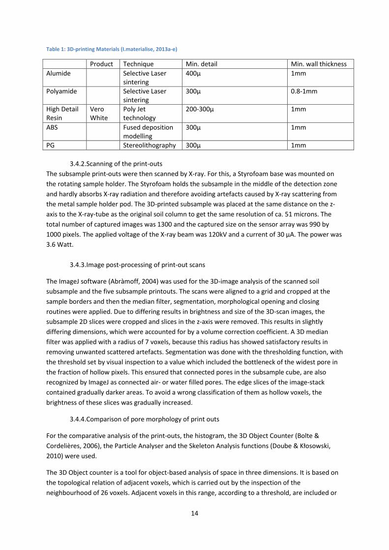
Table 1: 3D-printing Materials (I.materialise, 2013a-e)

Product Technique Min. detail Min. wall thickness Alumide Selective Laser

sintering 400µ 1mm

Polyamide Selective Laser sintering

300µ 0.8-1mm

High Detail Resin

Vero White

Poly Jet technology

200-300µ 1mm

ABS Fused deposition modelling

300µ 1mm

PG Stereolithography 300µ 1mm

3.4.2. Scanning of the print-outs The subsample print-outs were then scanned by X-ray. For this, a Styrofoam base was mounted on the rotating sample holder. The Styrofoam holds the subsample in the middle of the detection zone and hardly absorbs X-ray radiation and therefore avoiding artefacts caused by X-ray scattering from the metal sample holder pod. The 3D-printed subsample was placed at the same distance on the z-axis to the X-ray-tube as the original soil column to get the same resolution of ca. 51 microns. The total number of captured images was 1300 and the captured size on the sensor array was 990 by 1000 pixels. The applied voltage of the X-ray beam was 120kV and a current of 30 µA. The power was 3.6 Watt.

3.4.3. Image post-processing of print-out scans

The ImageJ software (Abràmoff, 2004) was used for the 3D-image analysis of the scanned soil subsample and the five subsample printouts. The scans were aligned to a grid and cropped at the sample borders and then the median filter, segmentation, morphological opening and closing routines were applied. Due to differing results in brightness and size of the 3D-scan images, the subsample 2D slices were cropped and slices in the z-axis were removed. This results in slightly differing dimensions, which were accounted for by a volume correction coefficient. A 3D median filter was applied with a radius of 7 voxels, because this radius has showed satisfactory results in removing unwanted scattered artefacts. Segmentation was done with the thresholding function, with the threshold set by visual inspection to a value which included the bottleneck of the widest pore in the fraction of hollow pixels. This ensured that connected pores in the subsample cube, are also recognized by ImageJ as connected air- or water filled pores. The edge slices of the image-stack contained gradually darker areas. To avoid a wrong classification of them as hollow voxels, the brightness of these slices was gradually increased.

3.4.4. Comparison of pore morphology of print outs

For the comparative analysis of the print-outs, the histogram, the 3D Object Counter (Bolte & Cordelières, 2006), the Particle Analyser and the Skeleton Analysis functions (Doube & Kłosowski, 2010) were used.

The 3D Object counter is a tool for object-based analysis of space in three dimensions. It is based on the topological relation of adjacent voxels, which is carried out by the inspection of the neighbourhood of 26 voxels. Adjacent voxels in this range, according to a threshold, are included or

14

excluded from the object (Bolte & Cordelières, 2006). The result of the 3D object counter results show a bounding box which encloses the “object”-pore. If the expansion of the bounding box along the z axis is equal to the length of the z-axis of the whole sample, a connection of the pore throughout the sample can be assumed.

The particle analyser is based on the 3D Object counter; the particle analyser provides the thickness of the object and the radii of a fitting ellipsoid. The volume, surface, coordinates of the pore-centroid, Euler-characteristics and the properties above were computed using the 3D Object Counter.

As explained above, the skeleton of a pore is the pore reduced to a single line. The branches of the skeleton are connected by nodes. A node connects two or more pore branches. Skeletonise 3D erodes an image to determine its skeleton and prepares it for skeleton analysis, which calculates branch length, counts junctions and prunes dead ends. From the skeleton, the longest shortest path, the single branch length and the Euclidean distance along the skeleton were of interest to calculate the tortuosity.

“Skeletonise 3D” from the BoneJ package was applied before the “Analyse Skeleton” function. Post processing of skeletons was also implemented, for example pruning of dead ends. Wildenschild & Sheppard (2013) claimed that the choice of skeletonisation method is less important than dealing with the difficulties of skeletonising non-bio pores such as fissures and cracks, which can have sheet-like shapes and therefore are represented insufficiently as a line by basic skeletons.

The longest shortest path is the length of the path through the skeleton which has the highest number of branches without loops. The length parameters of the skeleton were summarized from the lengths between two nodes. The tortuosity was calculated from the actual node length and straight line distance, which is the longest distance through a macropore network. For the mean tortuosity, all pore branches were accounted for (Luo et al., 2010). The term Euclidean distance is used here for the straight line distance between two nodes.

15

3.5. Hydraulic tests 3.5.1. Sessile drop wetting angle test

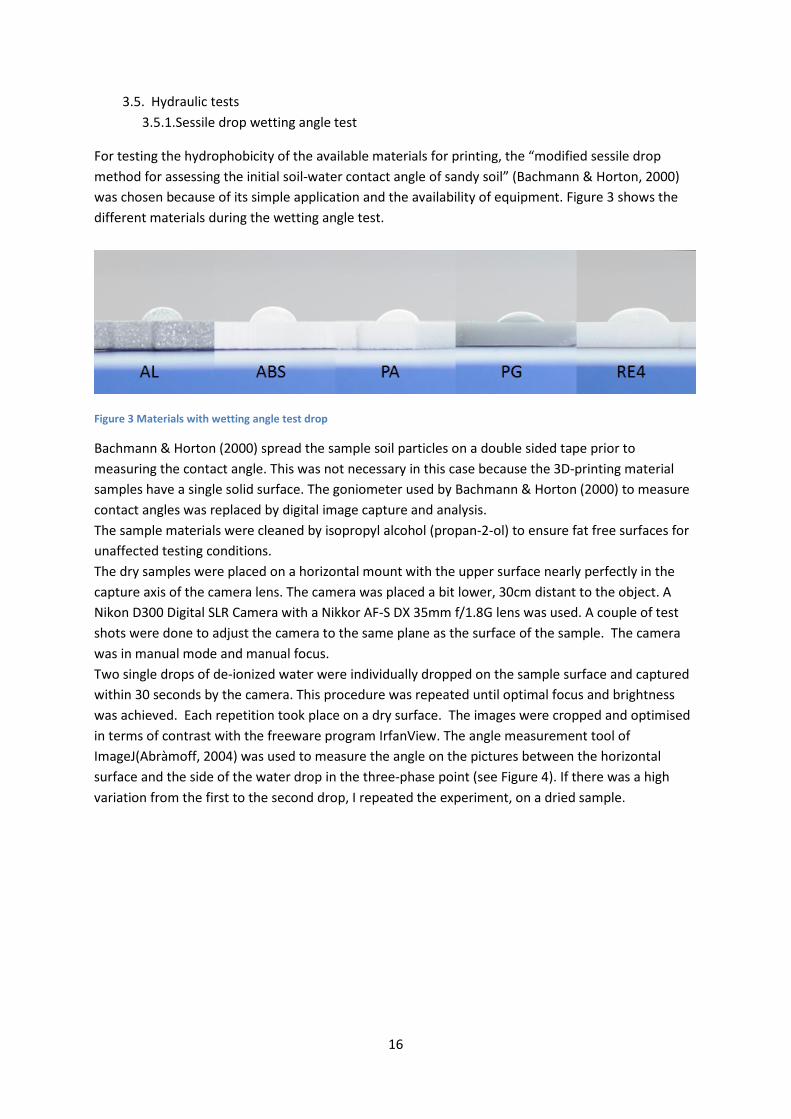
For testing the hydrophobicity of the available materials for printing, the “modified sessile drop method for assessing the initial soil-water contact angle of sandy soil” (Bachmann & Horton, 2000) was chosen because of its simple application and the availability of equipment. Figure 3 shows the different materials during the wetting angle test.

Figure 3 Materials with wetting angle test drop

Bachmann & Horton (2000) spread the sample soil particles on a double sided tape prior to measuring the contact angle. This was not necessary in this case because the 3D-printing material samples have a single solid surface. The goniometer used by Bachmann & Horton (2000) to measure contact angles was replaced by digital image capture and analysis. The sample materials were cleaned by isopropyl alcohol (propan-2-ol) to ensure fat free surfaces for unaffected testing conditions. The dry samples were placed on a horizontal mount with the upper surface nearly perfectly in the capture axis of the camera lens. The camera was placed a bit lower, 30cm distant to the object. A Nikon D300 Digital SLR Camera with a Nikkor AF-S DX 35mm f/1.8G lens was used. A couple of test shots were done to adjust the camera to the same plane as the surface of the sample. The camera was in manual mode and manual focus. Two single drops of de-ionized water were individually dropped on the sample surface and captured within 30 seconds by the camera. This procedure was repeated until optimal focus and brightness was achieved. Each repetition took place on a dry surface. The images were cropped and optimised in terms of contrast with the freeware program IrfanView. The angle measurement tool of ImageJ(Abràmoff, 2004) was used to measure the angle on the pictures between the horizontal surface and the side of the water drop in the three-phase point (see Figure 4). If there was a high variation from the first to the second drop, I repeated the experiment, on a dried sample.

16

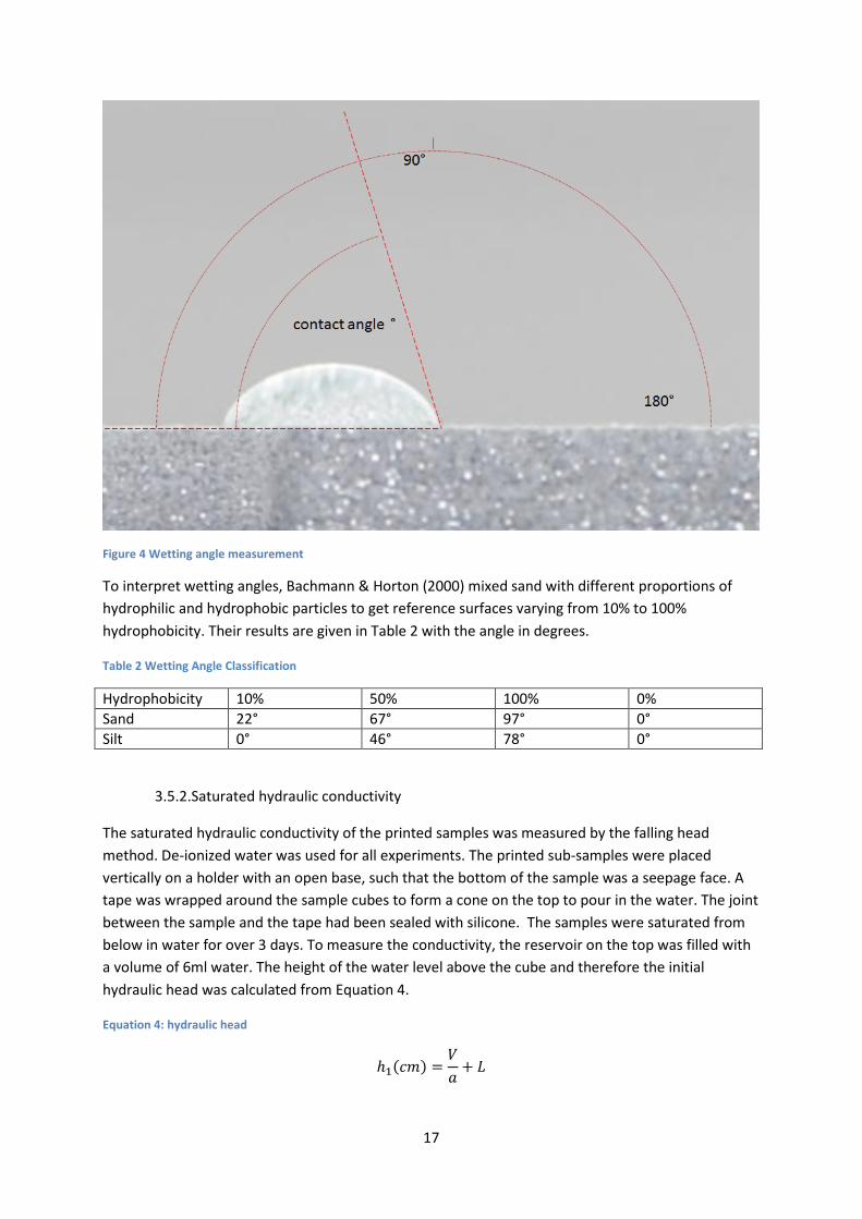
Figure 4 Wetting angle measurement

To interpret wetting angles, Bachmann & Horton (2000) mixed sand with different proportions of hydrophilic and hydrophobic particles to get reference surfaces varying from 10% to 100% hydrophobicity. Their results are given in Table 2 with the angle in degrees.

Table 2 Wetting Angle Classification

Hydrophobicity 10% 50% 100% 0% Sand 22° 67° 97° 0° Silt 0° 46° 78° 0°

3.5.2. Saturated hydraulic conductivity

The saturated hydraulic conductivity of the printed samples was measured by the falling head method. De-ionized water was used for all experiments. The printed sub-samples were placed vertically on a holder with an open base, such that the bottom of the sample was a seepage face. A tape was wrapped around the sample cubes to form a cone on the top to pour in the water. The joint between the sample and the tape had been sealed with silicone. The samples were saturated from below in water for over 3 days. To measure the conductivity, the reservoir on the top was filled with a volume of 6ml water. The height of the water level above the cube and therefore the initial hydraulic head was calculated from Equation 4.

Equation 4: hydraulic head

ℎ1(𝑐𝑚) =𝑉𝑎

+ 𝐿

17

Where h1 is the water height above the reference level (i.e. the bottom of the sample) at the beginning, V (cm3) is the volume of water in the reservoir, a (cm2) is the cross-sectional area of the sample cube and L is the height of the sample. Saturated hydraulic conductivity, k (cm s-1) was calculated using equation 5 (Assaad & Harb, 2013):

Equation 5: Falling head method

𝑘 �𝑐𝑚𝑠� =

𝐿∆𝑡∗ ln

ℎ1ℎ2

Where h2is the hydraulic head (cm) after the time ∆𝑡(𝑠). The distance between h1 and h2 is the same as L due to the experimental construction. A defined amount of water had been added in the cone on the top and the time until all water infiltrated, when the water level reached h2, was noted. The first run of the infiltration took 20 hours until the steady state infiltration started; therefore the infiltration experiment was repeated to get the duration of steady state flow. On repeating the infiltration experiments, some 3D-printed samples failed to infiltrate water in contrast to the first time. Therefore, the pores of the 3D-printed cubes were cleaned with pressurized de-ionized water to remove suspected bio-films and any remaining construction-aiding residual material that may have clogged the pores.

18

4. Results and Discussion 4.1. Pore morphology

Figure 5 shows the pore morphology in the 3D-Scans of the five print-outs in different materials as well as a 3D-scan of the soil sample itself. The renderings were done with a lower filtering threshold resolution of 50 voxels.

Figure 5 Sample Scan Results : scan of Prime Grey print(PG); High Detail Resin(RE4); Alumide(AL); Acrylnitril-Butadien-Styrol(ABS); Undisturbed Soil; scan of Polyamide print(PA)

A quick visual comparison shows that the ABS 3D-print sample has a very different pore structure because of the production process. The coiled structure in the ABS sample is hollow and appears as a huge macropore-network with a porosity of seven times higher than in the soil scan sample (Table 3). The shape of the printing aid residual structure is visible in Figure 5: ABS. The ends of the large macropores seen in the scan of the actual soil sample can just be seen on the front bottom and top of the right-hand side of the ABS print-out. To the largest macropore connected from the top to the bottom and the only one which is well shown in most scans is referred as reference pore.

The second largest pore in the soil sample, which goes alongside the large reference macropore quite straight vertically through the soil, has a mean diameter of 16 pixels (800µ) and a standard deviation of 3pixels(150µ). The only printed material sample containing this pore, and only in a rudimentary way, is the Polyamide sample. In Polyamide the pore is split up along its narrow parts and the mean diameter of the four fractions varies between 6 and 13 pixels which is equivalent to about 300-700µ.

PG RE4

ABS

AL

Soil PA

19

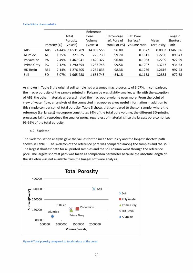
Table 3 Pore characteristics

Porosity (%)

Total Porosity (Voxels)

Reference Pore Volume (Voxels)

Percentage ref. Pore of total Por.(%)

Ref. Pore Surface/ Volume ratio

Mean Tortuosity

Longest Shortest Path

ABS ABS 24.44% 14 531 709 14 069 556 96.8% 0.3572 0.0003 1346.586 Alumide Al 1.25% 727 625 725 730 99.7% 0.1511 1.2200 899.43 Polyamide PA 2.49% 1 467 941 1 420 327 96.8% 0.1063 1.2209 922.99 Prime Grey PG 2.12% 1 290 394 1 283 748 99.5% 0.1207 1.3747 934.53 HD Resin RE4 2.14% 1 276 505 1 254 835 98.3% 0.1276 1.2616 997.43 Soil SO 3.07% 1 965 788 1 653 745 84.1% 0.1133 1.2855 972.68

As shown in Table 3 the original soil sample had a scanned macro porosity of 3.07%; in comparison, the macro porosity of the sample printed in Polyamide was slightly smaller, while with the exception of ABS, the other materials underestimated the macropore volume even more. From the point of view of water flow, an analysis of the connected macropores gives useful information in addition to this simple comparison of total porosity. Table 3 shows that compared to the soil sample, where the reference (i.e. largest) macropore constitutes 84% of the total pore volume, the different 3D-printing processes fail to reproduce the smaller pores, regardless of material, since the largest pore comprises 96-99% of the total porosity.

4.2. Skeleton

The skeletonisation analysis gave the values for the mean tortuosity and the longest shortest path shown in Table 3. The skeleton of the reference pore was compared among the samples and the soil. The largest shortest path for all printed samples and the soil column went through the reference pore. The largest shortest path was taken as comparison parameter because the absolute length of the skeleton was not available from the ImageJ software analysis.

Figure 6 Total porosity compared to total surface of the pores

Soil

Polyamide

Prime Gray

HD Resin

Alumide

80000

160000

240000

320000

400000

500000 1000000 1500000 2000000

Surf

ace[

Pixe

ls2 ]

Volume[Voxels]

Total Porosity

Soil

Polyamide

Prime Gray

HD Resin

Alumide

20

To simplify the analysis, the images were filtered to exclude smaller pores based on two criteria. The first criteria excluded all pores that were shorter than 1mm and the second excluded all pores with a surface area smaller than 314 pixel2, which equates roughly to a spherical pore with a diameter of 0.5 mm. Pore volumes smaller than this were assumed to be beyond the capability of exact 3D-printing. Pores smaller than 1 mm were assumed to be insignificant for water flow. The approximate pore length was estimated from the major radius of an equivalent ellipsoid fitting the pore.

Figure 7: Pore Volume Distribution shows the pore volume distributions of the five 3D-print material-samples and the soil after filtering as explained above. Each data series contains the soil pores from one sample.

For pores up to 500, 1000 and 10000 voxels in volume, the number of pores in the 3D-prints is generally significantly smaller than in the soil. However, the pore volume distributions for the Polyamide and ABS samples showed a similar trend to that in the scanned soil.

The largest pores in the sample are listed in Figure 7 in the column “more”. Each data series contains one very large pore which is the only connected macropore (“reference pore”) in the soil scan which is sufficiently well printed in all 3D-prints. The reference pore has a mean diameter of 35 pixels, which is equivalent to about 1.7mm. In the 3D-prints, this pore has a diameter of between 29 and 36 pixels. The Polyamide sample matched best to the size of the reference pore in the scanned soil sample.

0

5

10

15

20

25

30

35

40

500 1000 5000 10000 50000 100000 500000 1000000 More

Freq

uenc

y

Volume groups[Voxels]

Prime Grey

Alumide

HD-Resin

Polyamide

Soil

ABS

21

Figure 8 Parameters of largest pore in sample (Reference Pore):

The volume and surface area of the reference pore in four of the materials is plotted in Figure 8 and compared with that of the soil. The reference pore in ABS is not plotted in this graph because due to the different production process it is much bigger and therefore not directly comparable. Depending on the parameters, Figure 8 shows that three reference pores have the best fit with the soil reference pore. The surface-to-volume ratios in Table 3 shows that the reference pore of the Polyamide sample has the most compact shape, even more compact than the original soil pore, while Prime Grey has a more similar ratio to the soil reference.

Figure 9: Pore volume rank comparison of ABS Medium Pores with Soil and Polyamide

The residual structures in the ABS sample caused by the 3D-print technique (see figure 3) are not well sealed from the printed soil pores; therefore it was not possible to separate them during image analysis. Because the volume of the reference macropore in the ABS sample was not comparable with the reference pore in the soil column, macropores in the volume range from 1000-5000 voxels were sorted by size and plotted in Figure 9. The lower boundary was set to exclude single, spherical

Soil

Polyamide Prime Gray

HD Resin

Alumide 100000

120000

140000

160000

180000

200000

600 000 1 100 000 1 600 000

Surf

ace[

Pixe

ls2 ]

Volume[Voxels]

Reference Pore

Soil

Polyamide

Prime Gray

HD Resin

Alumide

800

1300

1800

2300

2800

3300

3800

4300

4800

Volu

me[

voxe

ls]

Pore rank

Material ABS Comparison

ABS

Soil

Polyamide

22

pores with an estimated radius of 7 pixels and a volume of about 600 voxels from the aiding structure. The upper boundary improves the presentation of the results by excluding the very large pores. Figure 7 shows that in this medium volume/size range, the pores in the printed material correlate very well in terms of volume and number with the pores in the soil scan.

4.3. Wetting angle & Durability

A test of the durability of the 3D-printed samples showed that all materials were resistant to dissolution in de-ionized water. In the beginning, some powder was dissolved from the Polyamide sample, which was found to be printing residue.

Table 4: Wetting Angle: The wetting angle (degree) the hydrophobicity is relative to the threshold of 67 degree; hydrophilic indicates by ∪; hydropobic indicated by ∩;

Sessile drop method

Sample Mean Wetting

Angle Std. Dev repetition

hydro-phobicity(67

deg)* ABS 54.9 5.66 4 ∪ Alumide 73.2 0.70 2 ∩ Polyamide 54.2 7.18 4 ∪ Prime Grey 68.7 7.67 3 ∩ HD-Resin 55.5 0.99 3 ∪

The results of the wetting angle test are shown in Table 4: Wetting AngleAll samples showed some degree of sub-critical water repellence, since wetting angles were larger than zero but smaller than 900. Alumide was relatively more hydrophobic, with a wetting angle of more than 70 degrees, while the resin and Polyamide materials can be considered as rather more hydrophilic with wetting angles smaller than 67 degrees (Bachmann & Horton, 2000). The wetting angle test had the difficulty that the visibility of the water drop and the transition between the surface of the material and the water drop depended on the material, which complicated the image-taking process and the analysis of wetting angles. A standard designated structure for mounting the camera and the sample horizontally would have improved the quality of the images. The test method could be also improved with a higher number of repetitions and by a closer consideration of surface structure and material property relations to wetting angle.

4.4. Infiltration

The infiltration tests suggested that the large macropore was physically connected between the top and bottom of the sample in only three of the five print-outs and High Detail Resin and Alumide had no infiltration. The tests also gave information on the saturated hydraulic conductivity for these three materials (see figure 8).

23

Figure 10 Hydraulic Conductivity

The saturated hydraulic conductivity measured by the falling head method differed between the different materials by order of magnitudes. The Prime Grey sample had the highest conductivity: the applied amount of water infiltrated within seconds. The ABS sample infiltrated the water within minutes and the Polyamide material took up to 5 hours to infiltrate 6 ml. Figure 8 shows that the hydraulic conductivity decreased slightly on repeating the infiltration, except for ABS where k increased. However, only 2 measurements were made for this material. The order of samples in the hydraulic conductivity measurements are in order with the ascending wetting angle. Never the less there is no direct effect of the wetting angle on the saturated hydraulic conductivity and the reason for a slow conductivity was not determined in this project.

The samples had been saturated from below for more than 3 days prior to the measurements. Nevertheless for Polyamide and ABS it took from hours to days until a constant flow was observed. The results for ABS are difficult to interpret, because they were not repeatable. This could be caused by limited connections between the macropore and the hollow aid structure. The measurements are prone to error in the case of a very high conductivity (short ∆t), because the time for the water surface to reach the reference level (h2) was not easy to determine accurately. It was also difficult to determine h2 in the case of very long infiltration times (∆t). The sealing of the reservoir to the sample is a critical aspect: the seal has to be perfect to ensure all water is going through the sample. The accuracy of the measurement could be improved with a larger reservoir on the top of the sample and a clearly distinguishable reference level, rather than using the sample surface as the reference level.

Printing aid materials and residual powder from the printing process may be the reason for the negligible hydraulic conductivity of the high-detail resin material and the low k values for ABS; it might also affect k for Polyamide as well. The influence and occurrence of bio-film in the pores was not assessed. The reasons for pore clogging might be answered by an X-ray scan of the different materials with a marker liquid showing how the pores are filled.

0,1

1

10

100

1000

1 2 3

k[cm

/h]

measurement

Hydraulic Conductivity

Prime Gray

Polyamide

ABS

24

5. Conclusion The images of the sample print-outs enabled an estimation of the effective lower limit of resolution of commercially-available 3D-printers. Current 3D-printing technology shows potential for reproducing soil macropores down to pore diameters of ca. 300-350 microns. This conclusion holds for all materials apart from ABS, for which the necessary information cannot be obtained from the image.

The saturated flow rates measured through the samples seem not to be correlated with the hydrophobicity of the printing materials, although the wetting angle is thought to have an impact on the rate of saturation. Therefore, materials with larger wetting angles are less appropriate for 3D-print of soil macropores. The role of wetting angles in regulating macropore flow needs more research.

Alumide has not only the largest wetting angle, but also comparably less printed pore volume than Polyamide, Prime Grey and high-detail resin. Furthermore there is no connectivity by any pore through the sample. Therefore, Alumide does not appear to be a suitable material for 3D-printing of soil macropores.

Polyamide, Prime Grey and high-detail resin have similar properties according to the digital image analysis. A slightly more detailed surface suggests that the high-detail resin may be the most appropriate material. The skeleton analysis showed a mean tortuosity for the High Detail Resin which was very similar to that of the scanned soil sample. However, no water flowed through the High Detail Resin sample during the infiltration tests and the optical comparison between the soil scan, the high-detail resin showed over exaggerated turns in the reference pore. A reasonably close match was found for Polyamide and the scanned soil sample in the results of the image analysis for total porosity and the largest macropore. The wetting angle measurements also indicated a low hydrophobicity for Polyamide. These parameters and the fact that Polyamide is the only material where the second largest connected pore was printed in a rudimentary way, would suggest that it is a favourable material.

ABS could be disqualified as a suitable printing material because pores were blocked by printing aid material and the printed pores were not sealed off from the hollow aiding structure. However, it may qualify for future research because the size distribution of medium-sized pores was similar to that in the soil sample and because it has a highly porous matrix.

For printing a soil with fewer small macropores or for applications where smaller macropores are negligible, Prime Grey may be the most appropriate 3D-printing material. Compared to Polyamide, the saturated hydraulic conductivity for Prime Grey is higher by more than three orders of magnitude. These two materials have the largest hydraulic conductivity, ignoring the uncertain results of the infiltration tests of the ABS print.

Cleaning the macropores and evaluation of appropriate chemical solvents for the residual material is one important step for further research. The problem of bio-films in 3D-printed objects has been mentioned for ABS (McCullough & Yadavalli, 2013) but needs further analysis.

3D-printing of undisturbed soil to reproduce macropores at the original scale is in principle possible, but the selection of the proper material and 3D-printing technique is crucial. The downside of

25

printing connected macropore-networks in 3D-printing material lies in the smaller scale. Bends and bottle-necks of macropores with an equivalent diameter of 300 microns have smaller diameters which are not printable or might easily become clogged. Therefore, at this stage of research in 3D-printing of artificial undisturbed soil for hydrological research, fully connected macropores throughout the sample are required.

Acknowledgements

I thank my supervisor John Koestel for his persistent support and countless productive discussions; my co-supervisor Andreas Schwen for his interesting and supplementing suggestions; Nicholas Jarvis for supreme editing of my thesis as well as my examiner Mats Larsbo;

I also want to thank my colleagues and friends for their input and support making the experience of writing the master’s thesis interesting and diverse.

26

References

Abràmoff, M., 2004. Image processing with ImageJ. Biophotonics …. Available at: http://igitur-archive.library.uu.nl/med/2011-0512-200507/UUindex.html [Accessed September 4, 2013].

Assaad, J.J. & Harb, J., 2013. Use of the Falling-head Method to Assess Permeability of Freshly Mixed Cementitious-based Materials. Journal of Materials in Civil Engineering, Volume 25(May), pp.1–11.

Bachmair, S., Weiler, M. & Nützmann, G., 2009. Controls of land use and soil structure on water movement: Lessons for pollutant transfer through the unsaturated zone. Journal of Hydrology, 369(3-4), pp.241–252.

Bachmann, J. & Horton, R., 2000. Modified sessile drop method for assessing initial soil–water contact angle of sandy soil. Soil Science Society of …, 64(April), pp.908–911. Available at: https://www.agronomy.org/publications/sssaj/abstracts/64/2/564 [Accessed June 27, 2013].

Baldwin, C.A. et al., 1996. Determination and Characterization of the Structure of a Pore Space from 3D Volume Images. Journal of colloid and interface science, 181(1), pp.79–92.

Bolte, S. & Cordelières, F.P., 2006. A guided tour into subcellular colocalization analysis in light microscopy. Journal of microscopy, 224(Pt 3), pp.213–32. Available at: http://www.ncbi.nlm.nih.gov/pubmed/17210054.

Doube, M. & Kłosowski, M., 2010. BoneJ: Free and extensible bone image analysis in ImageJ. Bone, 47(6), pp.1076–9. Available at: http://www.sciencedirect.com/science/article/pii/S8756328210014419 [Accessed June 18, 2013].

Feldkamp, L., Davis, L. & Kress, J., 1984. Practical cone-beam algorithm. JOSA A, 1(6), pp.612–619. Available at: http://www.opticsinfobase.org/abstract.cfm?&id=996 [Accessed June 18, 2013].

Feygin, M. et al., 1998. Laminated object manufacturing system. Available at: http://patent.ipexl.com/US/5730817.html.

Fisher Scientific, 2003. Prime Gray. Available at: https://fscimage.fishersci.com/msds/88249.htm [Accessed June 18, 2013].

GE, 2013a. DXR250 Detector. Available at: http://www.ge-mcs.com/en/radiography-x-ray/digital-x-ray/dxr250.html [Accessed June 19, 2013].

GE, 2013b. phoenix v|tome|x m. Available at: http://www.ge-mcs.com/en/radiography-x-ray/ct-computed-tomography/vtomex-m.html [Accessed June 19, 2013].

Gonzalez, R.C. & Woods, R.E., 2008. Digital Image Processing, Pearson Education.

Hull, C.W. & Lewis, C.W., 1986. Apparatus for production of three-dimensional objects by stereo- lithography. Available at: http://patent.ipexl.com/US/4575330.html.

I.materialise, 2013a. ABS. Available at: http://i.materialise.com/materials/abs [Accessed June 18, 2013].

27

I.materialise, 2013b. Alumide. Available at: http://i.materialise.com/materials/Alumide [Accessed June 18, 2013].

I.materialise, 2013c. High Detail Resin. Available at: http://i.materialise.com/materials/high-detail-resin [Accessed June 18, 2013].

I.materialise, 2013d. Polyamide. Available at: http://i.materialise.com/materials/Polyamide [Accessed June 18, 2013].

I.materialise, 2013e. Prime Gray. Available at: http://i.materialise.com/materials/prime-gray [Accessed June 18, 2013].

Jarvis, N.J., 2007. A review of non-equilibrium water flow and solute transport in soil macropores: principles, controlling factors and consequences for water quality. European Journal of Soil Science, 58(3), pp.523–546. Available at: http://doi.wiley.com/10.1111/j.1365-2389.2007.00915.x [Accessed May 23, 2013].

Jarvis, N.J. et al., 2012. Preferential Flow in a Pedological Perspective. In Hydropedology. Elsevier B.V., pp. 75–120.

Kapour, J., Sahoo, P. & Wong, A., 1985. A new method for gray-level picture thresholding using the entropy of the histogram. Computer vision, graphics, and image processing, 29(3), pp.273–285.

Karadimitriou, N.K. & Hassanizadeh, S.M., 2012. A Review of Micromodels and Their Use in Two-Phase Flow Studies. Vadose Zone Journal, 11(3). Available at: https://www.soils.org/publications/vzj/abstracts/11/3/vzj2011.0072 [Accessed May 28, 2013].

Li, C.H. & Tam, P.K.S., 1998. An iterative algorithm for minimum cross entropy thresholding. Pattern Recognition Letters, 19(8), pp.771–776. Available at: http://linkinghub.elsevier.com/retrieve/pii/S0167865598000579 [Accessed July 3, 2013].

Lindquist, W.B., 2002. Network flow model studies and 3D pore structure. Contemp. Math., 295, pp.355–366.

Luo, L., Lin, H. & Li, S., 2010. Quantification of 3-D soil macropore networks in different soil types and land uses using computed tomography. Journal of Hydrology, 393(1-2), pp.53–64. Available at: http://linkinghub.elsevier.com/retrieve/pii/S002216941000168X [Accessed June 6, 2013].

McCullough, E.J. & Yadavalli, V.K., 2013. Surface modification of fused deposition modeling ABS to enable rapid prototyping of biomedical microdevices. Journal of Materials Processing Technology, 213(6), pp.947–954. Available at: http://linkinghub.elsevier.com/retrieve/pii/S092401361300006X [Accessed June 12, 2013].

Olakanmi, E.O., 2013. Selective laser sintering/melting (SLS/SLM) of pure Al, Al–Mg, and Al–Si powders: Effect of processing conditions and powder properties. Journal of Materials Processing Technology, 213(8), pp.1387–1405. Available at: http://linkinghub.elsevier.com/retrieve/pii/S092401361300099X [Accessed June 29, 2013].

Otsu, N., 1979. A threshold selection method from gray-level histograms. IEEE TRANSACTIONS ON SYSTEMS MAN AND CYBERNETICS, 9(1), pp.62–66.

28

Otten, W. et al., 2012. Combining X-ray CT and 3D printing technology to produce microcosms with replicable, complex pore geometries. Soil Biology and Biochemistry, 51, pp.53–55. Available at: http://linkinghub.elsevier.com/retrieve/pii/S0038071712001472 [Accessed March 15, 2013].

Schwen, A. et al., 2011. Temporal dynamics of soil hydraulic properties and the water-conducting porosity under different tillage. Soil and Tillage Research, 113(2), pp.89–98.

Silin, D. et al., 2011. Microtomography and Pore-ScaleModeling of Two-Phase Fluid Distribution. Transport in porous media, 86(2), pp.495–515.

Singh, R., 2011. Process capability study of polyjet printing for plastic components. Journal of Mechanical Science and Technology, 25(4), pp.1011–1015. Available at: http://link.springer.com/10.1007/s12206-011-0203-8 [Accessed June 30, 2013].

Singh, S. et al., 2013. Optimization and Analysis of Mechanical Properties for Selective Laser Sintered Polyamide Parts. Materials and Manufacturing Processes, 28(2), pp.163–172. Available at: http://www.tandfonline.com/doi/abs/10.1080/10426914.2012.677901 [Accessed June 30, 2013].

Wildenschild, D. et al., 2002. Using X-ray computed tomography in hydrology : systems , resolutions , and limitations. Journal of Hydrology, 267, pp.285–297.

Wildenschild, D. & Sheppard, A.P., 2013. X-ray imaging and analysis techniques for quantifying pore-scale structure and processes in subsurface porous medium systems. Advances in Water Resources, 51, pp.217–246. Available at: http://linkinghub.elsevier.com/retrieve/pii/S0309170812002060 [Accessed March 15, 2013].

Windsheimer, H. et al., 2007. Laminated Object Manufacturing of Preceramic-Paper-Derived Si?SiC Composites. Advanced Materials, 19(24), pp.4515–4519. Available at: http://doi.wiley.com/10.1002/adma.200700789 [Accessed June 30, 2013].

Vogel, H.-J. & Roth, K., 2003. Moving through scales of flow and transport in soil. Journal of Hydrology, 272(1-4), pp.95–106. Available at: http://linkinghub.elsevier.com/retrieve/pii/S0022169402002573.

Zhou, H. et al., 2012. Effects of vegetation restoration on soil aggregate microstructure quantified with synchrotron-based micro-computed tomography. Soil and Tillage Research, 124, pp.17–23. Available at: http://www.sciencedirect.com/science/article/pii/S0167198712000931 [Accessed July 3, 2013].

29