1

Paper 354-2013

Virginia’s Best: How to Annotate County Names and Values on a State Map Anastasiya Osborne, Farm Service Agency (USDA), Washington, DC

ABSTRACT This paper describes a work project to annotate a Virginia state map with long county names and National Agricultural Statistics Service (NASS) data, using enhanced color and techniques to minimize map crowding. Displaying text and numeric data by county on a state map is different from displaying state-level data on a U.S. map. Long county names rather than two-letter state abbreviations require additional effort by a programmer to create a readable map. The SAS® code with %ANNOMAC, %CENTROID, PROC GPROJECT, PROC GMAP, and a 20-pattern color scheme were developed to create requested maps that showcased in color Virginia’s top agricultural counties. This paper is for intermediate level programmers.

INTRODUCTION The Virginia mapping project described in this paper was undertaken at the request of a Foreign Agricultural Service (FAS) employee and with approval from Farm Service Agency management. The goal was to use client-provided Microsoft Excel spreadsheets without state and county codes; match them with state and county codes for Virginia; create permanent SAS datasets; and finally generate five maps for the twenty leading Virginia counties across five categories. The categories were: total sales (market value of agricultural products sold including direct sales), acres, farm number, crop sales, and livestock sales. The SAS code required to accomplish those tasks was more difficult than the code described in the earlier paper (4). In 2011, the goal was to faithfully recreate twenty-two U.S. maps previously created in ArcGIS, with heavy restrictions on color choices and data formats. In this project, the client requested five maps with a flashy color scheme, big fonts, bright labels, and other means to attract the audience’s attention to significant agricultural output in Virginia’s counties. The project encountered several challenges. First, Excel files used as input data demand meticulous attention and can frustrate many a SAS user, as SAS-L archive proves, for example, http://listserv.uga.edu/cgi-bin/wa?A2=ind1208a&L=sas-l&F=&S=&P=14759. Intricate data formats, interesting long column headers, numeric versus character data in columns, and slight variations in the spelling of county names for each file challenged the author. Second, for the first time, the author confronted the problem of mapping counties on a state map. Learning %CENTROID solved this problem. Third, when the PDF file with each map appeared, the labels with the long county names and agricultural numbers often overlapped, three or four at a time, making the map unreadable. Several iterations were necessary to move the labels to the appropriate spots using the text-position described in the SAS Tech note (6). The resulting SAS program:

- uses %ANNOMAC to compile annotate macros before making labels in the center of each county; - uses %CENTROID to determine the coordinates for county centers; - extracts the top twenty counties by value; - inserts the chosen data into a map of Virginia counties; - eliminates the name of all other counties; - by trial and error, ensures that there is no crowding of labels and each can be seen and read; - uses a custom color scheme of twenty patterns to show the best-producing counties in each category.

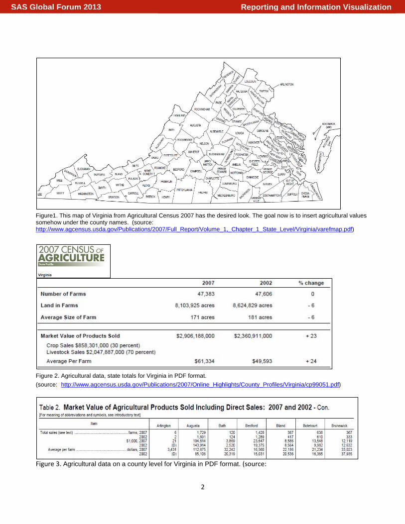
DESCRIPTION OF THE PROJECT In the beginning of the project, the author located the county map of Virginia and the data for insertion. The desired NASS data were publicly available, but in unfortunate PDF format. Fig.1 shows the county names and geography of Virginia. Fig.2. and Fig.3. provide the locations for the agricultural data on a state and county level. The goal appeared to be clear, but the method to achieve it was not. Surely this was not the first time a county map of one state was produced, but an extensive internet search could not locate any papers that discussed the labeling of several text strings in one text box on a county level.

Reporting and Information VisualizationSAS Global Forum 2013

2

Figure1. This map of Virginia from Agricultural Census 2007 has the desired look. The goal now is to insert agricultural values somehow under the county names. (source: http://www.agcensus.usda.gov/Publications/2007/Full_Report/Volume_1,_Chapter_1_State_Level/Virginia/varefmap.pdf)

Figure 2. Agricultural data, state totals for Virginia in PDF format. (source: http://www.agcensus.usda.gov/Publications/2007/Online_Highlights/County_Profiles/Virginia/cp99051.pdf)

Figure 3. Agricultural data on a county level for Virginia in PDF format. (source:

Reporting and Information VisualizationSAS Global Forum 2013

3

http://www.agcensus.usda.gov/Publications/2007/Full_Report/Volume_1,_Chapter_2_County_Level/Virginia/st51_2_002_002.pdf)

Interestingly, the list of files available for download contained only PDF files, http://www.agcensus.usda.gov/Publications/2007/Full_Report/Volume_1,_Chapter_1_State_Level/Virginia/. The next step was to contact NASS and request the data in a readable form, such as “VA county, state, county code, value.” As the website stated, information about NASS and its programs was available at www.nass.usda.gov, or by calling (800) 727-9540, or e-mailing nass@nass.usda.gov.

The author learned there were two options to get the data. First, NASS provides a downloadable tool for data extraction (Desktop Data Query Tool): http://www.agcensus.usda.gov/Publications/2007/Online_Highlights/Desktop_Application/index.asp. Second, another tool QuickStats from the NASS website, http://quickstats.nass.usda.gov, allows data users to customize a query against NASS database and create a spreadsheet file.

After trying both options, the author discovered that the data were still somewhat tabulated and not SAS-friendly, so NASS eventually supplied a custom-made represented in Fig. 4.

Figure 4. NASS-supplied CSV file with total sales for Virginia, on county level. Agricultural Census 2007.

The data column has numeric as well as character cells. The county names supplied in a “GEO” column are bunched together with the state name – but those problems were solvable. Later, the project became bigger and five maps were needed from an Excel file supplied by Bill Janis (Fig. 5. on next page).

Now, it made sense to read the Excel tabs one by one, merge them together by county name, and then merge them with the state and county names. Not so fast. The problems with this data source are visible. The file lacks state and county codes. The column headers are long. Crop data is formatted and has character values, and SAS read that column as character. Chesapeake City and Virginia Beach City are spelled together, but NOT in every tab – making it impossible to fully match them to the SAS coordinates by the county name. Those problems were solved, again, one by one, as the author encountered them. Misspelled cities provided the most entertainment.

At the end of creating a permanent SAS dataset, the first step of two (make good dataset; map it) was accomplished. Five datasets with twenty top-producing counties were ready to be mapped.

Reporting and Information VisualizationSAS Global Forum 2013

4

…

Figure 5. Excel file as input data.

%CENTROID Different versions of the map were produced, until it became clear that the SAS program tried to create a legend with the county names and values instead of mapping them to the county centers. A discussion with Mike Zdeb, a mapping expert, and a SAS Tech Support ticket allowed the author to learn about %CENTROID (3). This macro was added in SAS 9.0. As Darrell Massengill said, %CENTROID “creates a new dataset with the centroid of each polygon” for a map.

“%CENTROID (input-data-set, output-data-set, list-of-id-variables); input-data-set - specifies a map data set. output-data-set - contains the id variables and the X and Y variables.

Reporting and Information VisualizationSAS Global Forum 2013

5

list-of-id-variables - specifies the variables each of which is to be assigned the centroid coordinates of each observation in the input-data-set.” (3) In SAS 9.2, there is one observation for each unique set of ID values. However, as Robert Allison observed, in SAS 9.3, this situation is no longer the case (1). SAS 9.3 makes better centroids of map areas. Before, “the %CENTROID macro was a little over-simplistic, and only allowed you to specify the id variable, and then it would calculate the average centroid for all the points of each id.” Now, one can specify the desired segment for the centroid. “In most SAS maps, the first segment (segment=1) is the main/largest segment, you can now get the %centroid of just that main/largest segment: %CENTROID (namerica, centers, id, segonly=1 ); In most cases, this will produce a much 'better' centroid.” Therefore, to make a map, PROC GPROJECT was used to create a projected map, and then %ANNOMAC to get graphics commands to help with annotations. Then, %CENTROID was used to determine county centers. /*************************************************************************/ /* TIME TO MAP. Show the county and state boundaries for Virginia */ /*************************************************************************/ /* Generate the projected map of Virginia */ PROC JPROJECT data = maps.counties(where=(state=51)) /* Virginia */ Out = projVA ; id state county; RUN; /*NOTE: PARALLEL1 = 37.27160464. NOTE: PARALLEL2 = 38.734084745. NOTE: There were 22740 observations read from the data set MAPS.COUNTIES. WHERE state=51; NOTE: The data set WORK.PROJVA has 22740 observations and 6 variables. */ /* First, make the annotate macro available for use */ %ANNOMAC; /* Use the %CENTROID macro to find the county centers. */ %CENTROID( projVA /* input-data-set */ , VAcentersSAS /* output-data-set */ , state county /* list-of-id-variables */ ); /*NOTE: There were 136 observations read from the data set WORK.VACENTERS. NOTE: There were 22740 observations read from the data set WORK.PROJVA. */ /*Merge the centroids into the top twenty data */ DATA topcropsN20; /* dataset with total crop sales by county, 20 best*/ merge scropsN20(in=a) VAcentersSAS ; by state county; if a ; RUN; /* NOTE: There were 20 observations read from the data set WORK.SCROPSN20. NOTE: There were 136 observations read from the data set WORK.VACENTERSSAS. NOTE: The data set WORK.TOPCROPSN20 has 20 observations and 6 variables. After the regular mapping routine, the map looked like Fig.6. There was a joy in finally seeing a colorful map with the labels for requested counties, until a realization sank in – the map did not look quite right.

Reporting and Information VisualizationSAS Global Forum 2013

6

Figure 6. Unedited map of Virginia, showing top twenty VA counties with total value of crop sales, Census of Agriculture 2007. Several questionable spots with overlay of labels. Note three problem areas. Hanover and King William county labels clash; Pittsylvania-Halifax-Mecklenburg overlay makes it hard to read the labels; and Southampton-Isle of Wight-Suffolk City- Chesapeake City is one messy area needing immediate assistance with correct annotate positions.

HOW TO SPECIFY THE PLACEMENT OF TEXT-POSITIONS First, a regular code was run, to get Fig. 6. The usual hope was that the first run below would produce a palatable result, but with Virginia’s long county names that hope was vain for each of the five maps. The map with the crop sales was the most crowded, but four other maps (for total sales, acres, farm number, and livestock sales) also had to be adjusted. DATA annomap; length function color $8 text $30; retain xsys ysys '2' size 1.00 when 'a' color 'black' cbox 'yellow'; set topcropsN20 ; function='label'; position='B'; text=countyName; output; position='E';

Reporting and Information VisualizationSAS Global Forum 2013

7

text=put(crops, dollar12.0); output; RUN; Once the problems appear, it is time to employ a hands-on approach and decide in each case where the labels should be moved for better visibility. It happens by trial and error, though several iterations. It helps to check the annomap dataset before and after adjustment, to make sure that text-position for special cases changed. Regular text-positions are ‘B’ and ‘E’. Special cases can call for one of the nine text-positions (see (6) for more explanation)).

Figure 7. Text-position can be one of the characters 1 through 9, A through F, <, +, or >. DATA annomap; length function color $8 text $30; retain xsys ysys '2' size 1.00 when 'a' color 'black' cbox 'yellow'; set topcropsN20 ; /* Push down, middle */ if countyName = "SUFFOLK CITY" then do ; position='5'; text=countyName; output; position='8'; text=put(crops, dollar12.0); output; end ; /* Push left, up */ else if countyName in("PITTSYLVANIA", "SOUTHAMPTON") then do ; position='1'; text=countyName; output; position='4'; text=put(crops, dollar12.0); output; end ; /* Push down, right */ else if countyName in ("MECKLENBURG", "KING WILLIAM") then do ; position='6'; text=countyName; output; position='9'; text=put(crops, dollar12.0); output; end ;

Reporting and Information VisualizationSAS Global Forum 2013

8

/* Push up, center */ else if countyName in ("HALIFAX", "HANOVER") then do ; position='2'; text=countyName; output; position='5'; text=put(crops, dollar12.0); output; end ; /* Push up, right */ else if countyName = "CHESAPEAKE CITY" then do ; position='3'; text=countyName; output; position='6'; text=put(crops, dollar12.0); output; end ; /* Regular central position for two values */ else do ; function='label'; position='B'; text=countyName; output; position='E'; text=put(crops, dollar12.0); output; end ; RUN; /* NOTE: There were 20 observations read from the data set WORK.TOPSALES20. NOTE: The data set WORK.ANNOMAP has 40 observations and 15 variables. */

Fig. 8 displays the final map (see next page). We see clean readable labels with the county name and a value for crop sales. We also see a color scheme allowing for better visibility. Darker color represents a county with more sales. Northumberland County sets the lower bound with sales of $11,327 thousands of crop sales, shown in ivory, and Northampton County has the highest sales of $59,315, shown in vivid red. For each of the other four maps, a similar task was accomplished, making a map as is, and moving labels up and down, left and right in a similar fashion to separate the labels. As the maps were designed for a Power Point presentation, they were saved in a PNG format as well, because PNG files look better in Power Point than PDF files.

Reporting and Information VisualizationSAS Global Forum 2013

9

Figure 8. Final map of Virginia’s twenty top-producing counties for crop sales. Census of Agriculture 2007.

HOW TO MAP COUNTIES IN COLOR Now, let’s talk about the color scheme for the top ten and top twenty counties. In a 2009 paper (5), a color scheme for ten patterns was shared. Initially, the request for the Virginia maps project was to create maps with the top ten counties, making it ideal for the existing color scheme. However, once the number of requested counties increased to twenty, the author had to spend some time to make sure that each color appeared visibly different. If we were to make the map with crop sales for only top ten counties, the previous color scheme would look like in Fig.9. pattern1 v = msolid c = LemonChiffon; pattern2 v = msolid c = cxffcc00; /* Gold */ pattern3 v = msolid c = orange; pattern4 v = msolid c = cxd9892b; /* Brilliant Orange */ pattern5 v = msolid c = vpag; /* Very Pale Green */ pattern6 v = msolid c = YellowGreen ; /* Lighter Green */ pattern7 v = msolid c = MediumSeaGreen ; /* Darker Green */ pattern8 v = msolid c = brown; pattern9 v = msolid c = CX800000 ; /* Maroon */ pattern10 v = msolid c = CX33070F ; /* “Vivid Red” that shows as almost black */

Reporting and Information VisualizationSAS Global Forum 2013

10

Figure 9. Color scheme for ten patterns. Data are from a map for crop sales in Virginia but for top ten counties only. Fig. 10 displays a color scheme for twenty patterns, developed after several time-consuming iterations and consulting online resources for color suggestions, http://support.sas.com/techsup/technote/ts688/ts688.html and the ColorBrewer website, http://colorbrewer2.org/. In SAS, colors can be specified in several ways: by color name (Strong Pink), abbreviations (STPK), and RGB HEX codes (CXD9576E). More detailed description is beyond the scope of this paper, but interested SAS users can read already mentioned SAS tech support paper TS-688. pattern1 v = msolid c = CXFFFFF0 ; /* Ivory */ pattern2 v = msolid c = CXFFFFE0 ; /* Light Yellow */ pattern3 v = msolid c = CXFFFACD; /* Lemon Chiffon */ pattern4 v = msolid c = CXFFE4C4 ; /* Bisque */ pattern5 v = msolid c = CXFFDEAD ; /* Navajo White */ pattern6 v = msolid c = PINK ; /* Pink, CXFF0080 */ pattern7 v = msolid c = LIPK ; /* Light Pink CXE599A7 */ pattern8 v = msolid c = STPK ; /* Strong Pink CXD9576E */ pattern9 v = msolid c = MOY ; /* Moderate Yellow CX749938 */ pattern10 v = msolid c = BIY ; /* Brilliant Yellow CX8E996B */ pattern11 v = msolid c = STY ; /* Strong Yellow CX80BF1A */ pattern12 v = msolid c = DEY ; /* Deep Yellow CXAEE554 */ pattern13 v = msolid c = cxffcc00 ; /* Gold */ pattern14 v = msolid c = orange ; pattern15 v = msolid c = cxd9892b ; /* Brilliant Orange */ pattern16 v = msolid c = STO ; /* Strong Orange CXA66921 */ pattern17 v = msolid c = DEO ; /* Deep Orange CX80511A */ pattern18 v = msolid c = brown ; pattern19 v = msolid c = CX800000 ; /* Maroon */ pattern20 v = msolid c = CX33070F ; /* Vivid Red */

Figure 10. Color scheme for twenty patterns. Data are from the final map for crop sales in Virginia.

CONCLUSION This paper presented a detailed description of a real-life project that annotated a Virginia map with long county names and statistical data, and achieved colorful and readable data visualization. It offered the reader techniques on how to read input data in Excel files into SAS, how to use %CENTROID to find county centers, how to choose annotate positions for labels, and how to apply a color scheme for 20 patterns. The color scheme can be applied to a variety of projects in different industries. The SAS program is in the Appendix.

Reporting and Information VisualizationSAS Global Forum 2013

11

REFERENCES

1. Allison, Robert. “Robert Allison’s favorites of “What’s New in SAS v9.3 SAS/GRAPH.”2012. http://robslink.com/SAS/democd50/new_93_sas.htm#centroid

2. Heaton, Edward. “So, Your Data are in Excel!” SUGI31. www2.sas.com/proceedings/sugi31/020-31.pdf

3. Massengill, Darrell. “SAS Mapping: Technologies, Techniques, Tips and Tricks.” SUGI 28. http://support.sas.com/rnd/papers/sugi28/SASMapping.pdf

4. Osborne, Anastasiya. “Faking Esri ArcGIS maps in SAS®.” SAS Global Forum 2012. Available at: http://support.sas.com/resources/papers/proceedings12/263-2012.pdf

5. Osborne, Anastasiya. “Let Me Look At It! Graphic Presentation of Any Numeric Variable.” SAS Global Forum 2009.

support.sas.com/resources/papers/proceedings09/072-2009.pdf

6. The SAS Technical Note in SAS/GRAPH(R) 9.2: Reference, Second Edition. http://support.sas.com/documentation/cdl/en/graphref/63022/HTML/default/viewer.htm#annotate_position.htm

7. Zdeb, Mike. 2002. Maps Made Easy Using SAS. Cary, NC: SAS Institute Inc. SAS Institute Inc. 2004, SAS/GRAPH® Software: Reference, Version 9, Cary, NC: SAS Institute Inc.

ACKNOWLEDGMENTS Thank you, Bill Janis from the Foreign Agricultural Service, USDA, for sharing with me such an educational project on making state maps. My warmest thanks and gratitude extend to Mike Zdeb, SAS/GRAPH® Map Expert. I am also grateful to SAS Tech Support for promptly and courteously pointing me towards %CENTROID wonders. Thanks to Joy Harwood, the Economic and Policy Analysis Staff director at the Farm Service Agency, USDA; and to Terry Hickenbotham, my supervisor at the Farm Loan Analysis Group, for allowing me to work on and present this paper at SAS meetings and conferences. Sincere thanks to Bruce McWilliams, Terry Hickenbotham, Bill Janis, and Perry Watts for valuable and much appreciated comments.

CONTACT INFORMATION Your comments and questions are valued and highly encouraged. Contact the author at: Anastasiya Osborne Farm Service Agency, USDA 1400 Independence Ave, S.W. Washington, DC 20250-0506 Work Phone: 202-690-0446. E-mail: Anastasiya.Osborne@wdc.usda.gov SAS and all other SAS Institute Inc. product or service names are registered trademarks or trademarks of SAS Institute Inc. in the USA and other countries. ® indicates USA registration. Other brand and product names are trademarks of their respective companies.

Reporting and Information VisualizationSAS Global Forum 2013

12

APPENDIX 1. SAS PROGRAM “Create a Permanent DS for VA Counties.sas”

/********************************************************************************/ /* Name: Create a Permanent DS for VA Counties.sas */ /* Author: Anastasiya Osborne */ /* GOAL: From client-delivered Excel tables with no state and county codes, create permanent SAS datasets for further mapping of 20 most productive Virginia counties in each category: total sales, acres, farm number, crop sales, and livestock sales */ /* Output files: MC.Totagvalue20, MC.Acres20, MC.FarmN, MC.Crops20, MC.Livestock20. */ /* Plan: rename variables, make them numeric instead of character, match them with the state and county codes by county name, create subsets with twenty best performing counties, format the values, give them proper labels. Lots of mundane work. */ /* Input data: "C:\Bill Janis and Virginia\VA sales in Census2007.xls" */ /* Output: C:\Bill Janis and Virginia\ */ /********************************************************************************/ /* NOTE - SAS 9.2. can't do xlsx! Rename the file into xls. */ libname bj "H:\FSA SAS programs\Bill Janis Jan 9 2012" ; libname mc "C:\Bill Janis and Virginia" ; %let lryear=2007; %let mydate = August 5, 2012; filename OUT1 "C:\Bill Janis and Virginia\Census 2007 VA counties as of &mydate..pdf" ; LIBNAME new EXCEL "C:\Bill Janis and Virginia\VA Data for SAS May 25 2012.xls" HEADER=YES MIXED=YES; /* NOTE: Data source is connected in READ ONLY mode. NOTE: Libref NEW was successfully assigned as follows: Engine: EXCEL Physical Name: C:\Bill Janis and Virginia\VA Data for SAS May 25 2012.xls*/ /* A different Excel file with four variables needed to be mapped came from Bill Janis on April 20, 2012. An XLSX file was saved as XLS, and each worksheet was read separately: Total sales (market value of agricultural products sold including direct sales), acres, farm number, crop sales, and livestock sales. */ DATA mc.Farms_Acres (drop = F4 F5 F6); length county $25. ; set new."#Farms-Acres$"n; county = upcase(counties); RUN ; /*NOTE: There were 98 observations read from the data set NEW.'#Farms-Acres$'n. NOTE: The data set MC.FARMS_ACRES has 98 observations and 3 variables. */ DATA mc.TotAgValue (drop = F3 F4 F5 ); set new."Total Ag Value$"n; RUN ;

Reporting and Information VisualizationSAS Global Forum 2013

13

/* NOTE: There were 98 observations read from the data set NEW.'Total Ag Value$'n. NOTE: The data set MC.TOTAGVALUE has 98 observations and 2 variables. */ DATA mc.CropValue (drop = F3 F4 F5 ); set new."Crop Value$"n; RUN ; DATA mc.LivestockValue (drop = F3 F4 F5 ); Set new."Livestock Value$"n; RUN ; /* Since the input data does not have state and county codes, we need to match county names with their county codes. SAS has a dataset to create county names from a county code. Here is the opposite task. */ /* Step 1 - get a subset with county names from SAS-supplied data. */ DATA mc.StCountynames ; set maps.CNTYNAME (keep = state county statename countynm) ; where state = 51 ; /* Virginia */ RUN ; /* NOTE: There were 136 observations read from the data set MAPS.CNTYNAME. WHERE state=51; NOTE: The data set MC.STCOUNTYNAMES has 136 observations and 4 variables. */ %MACRO MYSORT (ds = ) ; proc sort data = &ds ; by counties ; run ; %MEND MYSORT ; %MYSORT (ds = mc.Farms_Acres ); %MYSORT (ds = mc.TotAgValue ); %MYSORT (ds = mc.CropValue ); %MYSORT (ds = mc.LivestockValue ); DATA fourvalues (rename = (county = countynm)); merge mc.Farms_Acres mc.TotAgValue mc.CropValue mc.LivestockValue ; by counties ; if counties = " " then delete ; RUN ; /* NOTE: There were 98 observations read from the data set MC.FARMS_ACRES. NOTE: There were 98 observations read from the data set MC.TOTAGVALUE. NOTE: There were 99 observations read from the data set MC.CROPVALUE. NOTE: There were 98 observations read from the data set MC.LIVESTOCKVALUE. NOTE: The data set WORK.FOURVALUES has 98 observations and 7 variables. */ /* This dataset has upcase "county" variable, and mixed case "counties" variable. */ PROC SORT sort data = fourvalues out = sfourvalues; by countynm ; RUN ; PROC SORT sort data = mc.StCountynames out = sStCountynames; by countynm ; RUN ;

Reporting and Information VisualizationSAS Global Forum 2013

14

/* Let's merge with the state and county codes. SAS-supplied data has many city codes that NASS data does not have values for. However, three cities are covered by NASS: Chesapeake City (cofips = 550), Suffolk City (800), and Virginia Beach City (810). */ DATA mc.VA2007 ; merge sfourvalues sStCountynames ; by countynm ; RUN ; /* NOTE: There were 98 observations read from the data set WORK.SFOURVALUES. NOTE: There were 136 observations read from the data set WORK.SSTCOUNTYNAMES. NOTE: The data set MC.VA2007 has 136 observations and 10 variables. */ PROC CONTENTS contents data = mc.VA2007 ; RUN ; /* Alphabetic List of Variables and Attributes # Variable Type Len Format Informat Label 9 COUNTY Num 6 County FIPS Code 2 Counties Char 19 $19. $19. Counties 6 Crops__including_ Num 8 Crops, including nursery nursery_and_gre and greenhouse crops $1,000 3 Farms_number Num 8 Farms number 4 Land_in_farms_acres Num 8 Land in farms acres 7 Livestock__poultry__ Num 8 Livestock, poultry, and their products and_their_pr $1,000 Farms by value of 5 Market_value_of_ Num 8 Market value of agricultural agricultural_pro products sold $1,000 8 STATE Num 5 State FIPS Code 10 STATENAME Char 20 Name of State 1 countynm Char 25 County Name */ DATA mc.VA2007ready ; set mc.VA2007 ; rename Market_value_of_agricultural_pro = totsales Land_in_farms_acres = acres Farms_number = farmN Crops__including_nursery_and_gre = Crops Livestock__poultry__and_their_pr = Livestock ; RUN ; PROC CONTENTS contents data = mc.VA2007ready ; RUN ; /* Alphabetic List of Variables and Attributes # Variable Type Len Format Informat Label 9 COUNTY Num 6 County FIPS Code 2 Counties Char 19 $19. $19. Counties

Reporting and Information VisualizationSAS Global Forum 2013

15

6 Crops Num 8 Crops, including nursery and greenhouse crops $1,000 7 Livestock Num 8 Livestock, poultry, and their products $1,000 Farms by value of 8 STATE Num 5 State FIPS Code 10 STATENAME Char 20 Name of State 4 acres Num 8 Land in farms acres 1 countynm Char 25 County Name 3 farmN Num 8 Farms number 5 totsales Num 8 Market value of agricultural products sold $1,000 */ /*************************************************************************/ /* Out of five varibles, two required a comma format (acreage and farm number), and three - a dollar format (totsales, cropsales, livestock sales).*/ /* Here, the code for only one of the five datasets is shown. */ /*************************************************************************/ /* Create top 20 for crops */ DATA crops ; set mc.VA2007ready (keep = state county countynm crops) ; RUN ; PROC SORT data = crops out = scrops; by descending crops ; RUN ; DATA MC.CROPS20 ; set scrops (firstobs = 1 obs = 20); format crops dollar12.0 ; label crops = "Market Value of Crops, Including Nursery and Greenhouse Crops, $1,000" ; RUN ; … /* repeate with variations for the other four variables */ /* End of Create a permanent DS for VA counties.sas */

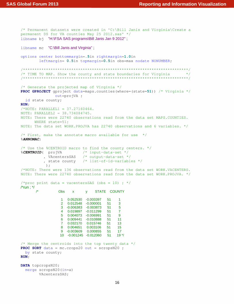
APPENDIX 2. SAS PROGRAM “Mapping Crop Sales in VA.sas”

/***************************************************************************/ /* Program: Mapping crop sales in VA.sas */ /* Author: Anastasiya Osborne */ /* Date: Aug 5, 2012 */ /* GOAL: Make a map of total sales for 20 leading Virginia counties */ /* Step 2. Step 1: "C:\Bill Janis and Virginia\Create a permanent DS for VA counties.sas */ /* Input data: "C:\Bill Janis and Virginia\MC.Totagvalue20, MC.Acres20, MC.FarmN, MC.Crops20, MC.Livestock20 */ /* Original data: "C:\Bill Janis and Virginia\VA sales in Census2007.xls" */ /* Output: C:\Bill Janis and Virginia\ */ /***************************************************************************/ /* NOTE - SAS 9.2 can't do xlsx! Rename the file into xls. */

Reporting and Information VisualizationSAS Global Forum 2013

16

/* Permanent datasets were created in "C:\Bill Janis and Virginia\Create a permanent DS for VA counties May 25 2012.sas" */ libname bj "H:\FSA SAS programs\Bill Janis Jan 9 2012" ; libname mc "C:\Bill Janis and Virginia" ; options center bottommargin=.5in rightmargin=1.0in leftmargin= 0.5in topmargin=0.5in obs=max nodate NONUMBER; /************************************************************************/ /* TIME TO MAP. Show the county and state boundaries for Virginia */ /************************************************************************/ /* Generate the projected map of Virginia */ PROC GPROJECT gproject data=maps.counties(where=(state=51)) /* Virginia */ out=projVA ; id state county; RUN; /*NOTE: PARALLEL1 = 37.27160464. NOTE: PARALLEL2 = 38.734084745. NOTE: There were 22740 observations read from the data set MAPS.COUNTIES. WHERE state=51; NOTE: The data set WORK.PROJVA has 22740 observations and 6 variables. */ /* First, make the annotate macro available for use */ %ANNOMAC; /* Use the %CENTROID macro to find the county centers. */ %CENTROID( projVA /* input-data-set */ , VAcentersSAS /* output-data-set */ , state county /* list-of-id-variables */ ); /*NOTE: There were 136 observations read from the data set WORK.VACENTERS. NOTE: There were 22740 observations read from the data set WORK.PROJVA. */ /*proc print data = vacentersSAS (obs = 10) ; */ /*run ; */ /* Obs x y STATE COUNTY 1 0.052530 -0.003397 51 1 2 0.012548 -0.000001 51 3 3 -0.006383 -0.003873 51 5 4 0.019897 -0.011299 51 7 5 0.004073 -0.006991 51 9 6 0.009441 -0.010888 51 11 7 0.032170 0.015746 51 13 8 0.004651 0.003106 51 15 9 -0.003609 0.000855 51 17 10 -0.001245 -0.012060 51 19 */ /* Merge the centroids into the top twenty data */ PROC SORT data = mc.crops20 out = scropsN20 ; by state county; RUN; DATA topcropsN20; merge scropsN20(in=a) VAcentersSAS;

Reporting and Information VisualizationSAS Global Forum 2013

17

by state county; if a ; RUN; /* NOTE: There were 20 observations read from the data set WORK.SCROPSN20. NOTE: There were 136 observations read from the data set WORK.VACENTERSSAS. NOTE: The data set WORK.TOPCROPSN20 has 20 observations and 6 variables. */ /* Advice: check annomap dataset, to make sure that text position for special cases changed! Also, check that the number of observations is not higher than expected. Here, we expect two labels for each of the top 20 counties - therefore, only 40 observations. If it's higher, there will be unnecessary labels. */ DATA annomap; length function color $8 text $30; retain xsys ysys '2' size 1.00 when 'a' color 'black' cbox 'yellow'; set topcropsN20 ; /* Push down, middle */ if countyName = "SUFFOLK CITY" then do ; position='5'; text=countyName; output; position='8'; text=put(crops, dollar12.0); output; end ; /* Push left, up */ else if countyName in("PITTSYLVANIA", "SOUTHAMPTON") then do ; position='1'; text=countyName; output; position='4'; text=put(crops, dollar12.0); output; end ; /* Push down, right */ else if countyName in ("MECKLENBURG", "KING WILLIAM") then do ; position='6'; text=countyName; output; position='9'; text=put(crops, dollar12.0); output; end ; /* Push up, center */ else if countyName in ("HALIFAX", "HANOVER") then do ; position='2'; text=countyName; output; position='5'; text=put(crops, dollar12.0);

Reporting and Information VisualizationSAS Global Forum 2013

18

output; end ; /* Push up, right */ else if countyName = "CHESAPEAKE CITY" then do ; position='3'; text=countyName; output; position='6'; text=put(crops, dollar12.0); output; end ; /* Central position for two values */ else do ; function='label'; position='B'; text=countyName; output; position='E'; text=put(crops, dollar12.0); output; end ; RUN ; /* NOTE: There were 20 observations read from the data set WORK.TOPSALES20. NOTE: The data set WORK.ANNOMAP has 40 observations and 15 variables. */ PROC PRINT data = annomap (firstobs = 22 ) ; RUN ; /* This is the print out before the adjustment. All positions show B and E. */ /* Obs function color text xsys ysys size when cbox countyName 22 label black $21,228 2 2 1 a yellow MECKLENBURG 23 label black NORTHAMPTON 2 2 1 a yellow NORTHAMPTON 24 label black $59,315 2 2 1 a yellow NORTHAMPTON 25 label black NORTHUMBERLAND 2 2 1 a yellow NORTHUMBERLAND 26 label black $11,327 2 2 1 a yellow NORTHUMBERLAND 27 label black ORANGE 2 2 1 a yellow ORANGE 28 label black $50,673 2 2 1 a yellow ORANGE 29 label black PITTSYLVANIA 2 2 1 a yellow PITTSYLVANIA 30 label black $23,409 2 2 1 a yellow PITTSYLVANIA 31 label black ROCKINGHAM 2 2 1 a yellow ROCKINGHAM 32 label black $20,047 2 2 1 a yellow ROCKINGHAM 33 label black SOUTHAMPTON 2 2 1 a yellow SOUTHAMPTON 34 label black $27,500 2 2 1 a yellow SOUTHAMPTON 35 label black WESTMORELAND 2 2 1 a yellow WESTMORELAND 36 label black $24,267 2 2 1 a yellow WESTMORELAND 37 label black CHESAPEAKE CITY 2 2 1 a yellow CHESAPEAKE CITY 38 label black $30,956 2 2 1 a yellow CHESAPEAKE CITY 39 label black SUFFOLK CITY 2 2 1 a yellow SUFFOLK CITY 40 label black $42,222 2 2 1 a yellow SUFFOLK CITY Obs Crops state county x y position 22 $21,228 51 117 0.015997 -0.022398 E 23 $59,315 51 131 0.050628 -0.010998 B 24 $59,315 51 131 0.050628 -0.010998 E

Reporting and Information VisualizationSAS Global Forum 2013

19

25 $11,327 51 133 0.042514 -0.001891 B 26 $11,327 51 133 0.042514 -0.001891 E 27 $50,673 51 137 0.019527 0.004583 B 28 $50,673 51 137 0.019527 0.004583 E 29 $23,409 51 143 0.001122 -0.020319 B 30 $23,409 51 143 0.001122 -0.020319 E 31 $20,047 51 165 0.007307 0.009193 B 32 $20,047 51 165 0.007307 0.009193 E 33 $27,500 51 175 0.033362 -0.021078 B 34 $27,500 51 175 0.033362 -0.021078 E 35 $24,267 51 193 0.035524 0.002593 B 36 $24,267 51 193 0.035524 0.002593 E 37 $30,956 51 550 0.044827 -0.021904 B 38 $30,956 51 550 0.044827 -0.021904 E 39 $42,222 51 800 0.039953 -0.021523 B 40 $42,222 51 800 0.039953 -0.021523 E */ /****************************************************************/ /***** Preparation for maps ***/ /****************************************************************/ goptions reset=all rotate=landscape ; /* The way it's printed on a page */ legend1 across= 8 /*Shows the layout of the legend patterns */ mode= share shape=bar (3,2) position=(top center outside) origin= (5,5)pct /* As of July 22, 2012 */; pattern1 v = msolid c = CXFFFFF0 ; /* Ivory */ pattern2 v = msolid c = CXFFFFE0 ; /* Light Yellow */ pattern3 v = msolid c = CXFFFACD; /* Lemon Chiffon */ pattern4 v = msolid c = CXFFE4C4 ; /* Bisque */ pattern5 v = msolid c = CXFFDEAD ; /* Navajo White */ pattern6 v = msolid c = PINK ; /* Pink, CXFF0080 */ pattern7 v = msolid c = LIPK ; /* Light Pink CXE599A7 */ pattern8 v = msolid c = STPK ; /* Strong Pink CXD9576E */ pattern9 v = msolid c = MOY ; /* Moderate Yellow CX749938 */ pattern10 v = msolid c = BIY ; /* Brilliant Yellow CX8E996B */ pattern11 v = msolid c = STY ; /* Strong Yellow CX80BF1A */ pattern12 v = msolid c = DEY ; /* Deep Yellow CXAEE554 */ pattern13 v = msolid c = cxffcc00 ; /* Gold */ pattern14 v = msolid c = orange ; pattern15 v = msolid c = cxd9892b ; /* Brilliant Orange */ pattern16 v = msolid c = STO ; /* Strong Orange CXA66921 */ pattern17 v = msolid c = DEO ; /* Deep Orange CX80511A */ pattern18 v = msolid c = brown ; pattern19 v = msolid c = CX800000 ; /* Maroon */ pattern20 v = msolid c = CX33070F ; /* Vivid Red */ /* White space around map; from Mike Zdeb. */ title1 ls=1; title2 a=90 ls=2; title3 a=-90 ls=2; ods listing close; ods results off;

Reporting and Information VisualizationSAS Global Forum 2013

20

ods pdf file= "C:\Bill Janis and Virginia\Edited Crop Sales - Census 2007 VA counties as of August 5 2012.pdf" notoc ; ods escapechar='^'; /* If I used the first statement in my code, this means that anytime ODS encounters the caret (^) it will interpret whatever follows the caret (^) to be a sequence or string of control */ title; PROC GMAP data = scropsN20 /* response data */ map = projVA /* boundary data - just the centroids for VA counties, projected */ all ; /*The ALL option is needed. Without it, only one county would be displayed. */ id state county; choro crops / discrete

annotate = annomap /* annotation data, with the county names and total sales */

cempty=black coutline=black ctext=black legend = legend1 ; label crops = "Crop Sales, $1,000:" ; note height=14 pt f = swissb ls = 1 j=c "Virginia: Twenty Counties with the Highest Value of Crop Sales" j=c "Census of Agriculture 2007" ; RUN; QUIT; pattern ; ods pdf close; ods results on; ods listing; /* End of "Mapping crop sales in VA.sas*/

Reporting and Information VisualizationSAS Global Forum 2013