Digitales Video

1

3. SAMPLING THEORY

3.1. INTRODUCTION

This chapter reviews the principal ideas of digital filtering and sampling theory. A brief review is appropriate in order to grasp the key issues relevant to the resampling and antialiasing stages that follow. Both stages share the common two-fold problem addressed by sampling theory: Given a continuous input signal g(x) and its sampled counterpart gs(x), are the samples of gs(x) sufficient to exactly describe g(x)? If so, how can g(x) be reconstructed from gs(x)? This problem is known as signal reconstruction. The solution lies in the frequency domain whereby spectral analysis is used to examine the spectrum of the sampled data.

The conclusions derived from examining the reconstruction problem will prove to be directly useful for resampling and indicative of the filtering necessary for antialiasing. Sampling theory thereby provides an elegant mathematical framework in which to assess the quality of reconstruction, establish theoretical limits, and predict when it is not possible.

In order to better motivate the importance of sampling theory, we demonstrate its role with the following examples. A checkerboard texture is shown projected onto an oblique planar surface in Figure 3.1. The image exhibits two forms of artifacts: jagged edges and moire patterns. Jagged edges are prominent toward the bottom of the image, where the input checkerboard undergoes magnification. The moire patterns, on the other hand, are noticable at the top, where minification (compression) forces many input pixels to occupy fewer output pixels.

Figure 3.1 Oblique checkerboard (unfiltered)

Figure 3.1 was generated by projecting the center of each output pixel into the checkerboard and sampling (reading) the value at the nearest input pixel. This point sampling method performs poorly, as is evident by the objectionable results of Figure 3.1. This conclusion is reached by sampling theory as well. Its role here is to precisely quantify this phenomena and to prescribe a solution. Figure 3.2 shows the same mapping with improved results. This time the necessary steps were taken to preclude artifacts.

Digitales Video

2

3.2. SAMPLING

The images will be taken as one-dimensional signals, i.e., a single scanline image. Recall that the continuous signal, f(x), is presented to the imaging system. Due to the point spread function of the imaging device, the degraded output g(x) is a bandlimited signal with attenuated high frequency components. Since visual detail directly corresponds to spatial frequency, it follows that g(x) will have less detail than its original counterpart f(x). The frequency content of g(x) is given by its spectrum, G(f), as determined by the Fourier transform.

3.1

Figure 3.2 Oblique checkerboard (filtered).

The magnitude spectrum of a signal is shown in Figure 3.3 . It shows a concentration of energy in the low-frequency range, tapering off toward the higher frequencies. Since there are no frequency components beyond fmax, the signal is said to be bandlimited to frequency fmax.

Figure 3.3 Spectrum G(f).

Digitales Video

3

The continuous output g(x) is then digitized by an ideal impulse sampler, the comb function, to get the sampled signal gs(x). The ideal 1-D sampler is given as

3.2

where δ is the familiar impulse function and Ts is the sampling period. The running index n is used with δ to define the impulse train of the comb function. We now have

3.3

Taking the Fourier transform of gs(x) yields

3.4

where fs is the sampling frequency and * denotes convolution. The above equations make use of the following well-known properties of Fourier transforms:

Multiplication in the spatial domain corresponds to convolution in the frequency domain. Therefore, Eq. 3.3 gives rise to a convolution in Eq. 3.4. The Fourier transform of an impulse train is itself an impulse train, giving us Eq. 3.4. The spectrum of a signal sampled with frequency fs (Ts = 1/fs) yields the original spectrum replicated in the frequency domain with period fs (Eq. 3.4).

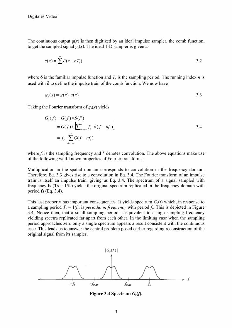
This last property has important consequences. It yields spectrum Gs(f) which, in response to a sampling period Ts = 1/fs, is periodic in frequency with period fs. This is depicted in Figure 3.4. Notice then, that a small sampling period is equivalent to a high sampling frequency yielding spectra replicated far apart from each other. In the limiting case when the sampling period approaches zero only a single spectrum appears a result consistent with the continuous case. This leads us to answer the central problem posed earlier regarding reconstruction of the original signal from its samples.

Figure 3.4 Spectrum Gs(f).

Digitales Video

4

3.3. RECONSTRUCTION

The above result reveals that the sampling operation has left the original input spectrum intact, merely replicating it periodically in the frequency domain with a spacing of fs. This allows us to rewrite Gs(f) as a sum of two terms, the low frequency (baseband) and high frequency components. The baseband spectrum is exactly G(f), and the high frequency components, Ghigh(f), consist of the remaining replicated versions of G(f) that constitute harmonic versions of the sampled image.

3.5

Exact signal reconstruction from sampled data requires us to discard the replicated spectra Ghigh(f), leaving only G(f), the spectrum of the signal we seek to recover. This is a crucial observation in the study of sampled-data systems.

3.3.1. Reconstruction Conditions

The only provision for exact reconstruction is that G(f) be undistorted due to overlap with Ghigh(f). Two conditions must hold for this to be true:

• The signal must be bandlimited. This avoids spectra with infinite extent that are impossible to replicate without overlap.

• The sampling frequency fs must be greater than twice the maximum frequency fmax, present in the signal. This minimum sampling frequency, known as the Nyquist rate, is the minimum distance between the spectra copies, each with bandwidth fmax.

The first condition merely ensures that a sufficiently large sampling frequency exists that can be used to separate replicated spectra from each other. Since all imaging systems impose a bandlimiting filter in the form of a point spread function, this condition is always satisfied for images captured through an optical system.

Note that this does not apply to synthetic images, e.g., computer-generated imagery. This does not include the shot noise that may be introduced by digital scanners. The second condition proves to be the most revealing statement about reconstruction. It answers the problem regarding the sufficiency of the data samples to exactly reconstruct the continuous input signal. It states that exact reconstruction is possible only when fs > fNyquist, where fNyquist = 2fmax. Collectively, these two conclusions about reconstruction form the central message of sampling theory, as pioneered by Claude Shannon in his landmark papers on the subject [Shannon 48, 49].

3.3.2. Ideal Low-Pass Filter

We now turn to the second central problem: Given that it is theoretically possible to perform reconstruction, how may it be done? The answer lies with our earlier observation that sampling merely replicates the spectrum of the input signal, generating Ghigh(f) in addition to G(f). Therefore, the act of reconstruction requires us to completely suppress Ghigh(f). This is done by multiplying Gs(f) with H(f), given as

Digitales Video

5

3.6

H(f) is known as an ideal low-pass filter and is depicted in Figure 3.5, where it is shown suppressing all frequency components above fmax. This serves to discard the replicated spectra Ghigh(f). It is ideal in the sense that the fmax cut-off frequency is strictly enforced as the transition point between the transmission and complete suppression of frequency components.

Figure 3.5 Ideal low-pass filter H(f).

Realistic sampling techniques must sample at rates far above the Nyquist frequency in order to avoid the nonideal elements that enter into the process (e.g., sampling with a narrow pulse rather than an impulse). This has more serious consequences for synthetic images that can indeed be sampled with a perfect comb function.

3.3.3. Sinc Function

In the spatial domain, the ideal low-pass filter is derived by computing the inverse Fourier transform of H(f). This yields the sinc function shown in Figure 3.6. It is defined as

Figure 3.6 The sinc function.

The reader should note the reciprocal relationship between the height and width of the ideal low-pass filter in the spatial and frequency domains. Let A denote the amplitude of the sinc function, and let its zero crossings be positioned at integer multiples of 1/2W. The spectrum of this sinc function is a rectangular pulse of height A/2W and width 2W, with frequencies ranging from -W to W. In our example above, A = 1 and W = fmax=.5 cycles/pixel. This value for W is derived from the fact that digital images must not have more than one half cycle per pixel in order to conform to the Nyquist rate.

Digitales Video

6

The sinc function is one instance of a large class of functions known as cardinal splines, which are interpolating functions defined to pass through zero at all but one data sample, where they have a value of one. This allows them to compute a continuous function that passes through the uniformly-spaced data samples.

Since multiplication in the frequency domain is identical to convolution in the spatial domain, sinc(x) represents the convolution kernel used to evaluate any point x on the continuous input curve g given only the sampled data gs.

3.1

Equation 3.7 highlights an important impediment to the practical use of the ideal low-pass filter. The filter requires an infinite number of neighboring samples (i.e., an infinite filter support) in order to precisely compute the output points. This is, of course, impossible owing to the finite number of data samples available. However, truncating the sinc function allows for approximate solutions to be computed at the expense of undesirable "ringing", i.e., ripple effects. These artifacts, known as the Gibbs phenomenon, are the overshoots and undershoots caused by reconstructing a signal with truncated frequency terms. The two rows in Figure 3.7 show that truncation in one domain leads to ringing in the other domain. This indicates that a truncated sinc function is actually a poor reconstruction filter because its spectrum has infinite extent and thereby fails to bandlimit the input.

Figure 3.7 Truncation in one domain causes ringing the other domain.

In response to these difficulties, a number of approximating algorithms have been derived, offering a tradeoff between precision and computational expense. These methods permit local solutions that require the convolution kernel to extend only over a small neighborhood. The drawback, however, is that the frequency response of the filter has some undesirable properties. In particular, frequencies below fmax are tampered, and high frequencies beyond fmax are not fully suppressed. Thus, nonideal reconstruction does not permit us to exactly recover the continuous underlying signal without artifacts. As we shall see, though, there are ways of ameliorating these effects. The problem of nonideal reconstruction receives a great deal of attention in the literature due to its practical significance.

Digitales Video

7

3.4. NONIDEAL RECONSTRUCTION

The process of nonideal reconstruction is depicted in Figure 3.8, which indicates that the input signal satisfies the two conditions necessary for exact reconstruction. First, the signal is bandlimited since the replicated copies in the spectrum are each finite in extent. Second, the sampling frequency exceeds the Nyquist rate since the copies do not overlap. However, this is where our ideal scenario ends. Instead of using an ideal low-pass filter to retain only the baseband spectrum components, a nonideal reconstruction filter is shown in the figure.

Figure 3.8 Nonideal reconstruction.

The filter response Hr(f) eviates from the ideal response H(f) shown inFigure 3.5. In particular, Hr(f) does not discard all frequencies beyond fmax. Furthermore, that same filter is shown to attenuate some frequencies that should have remained intact. This brings us to the problem of assessing the quality of a filter.

The accuracy of a reconstruction filter can be evaluated by analyzing its frequency domain characteristics. Of particular importance is the filter response in the passband and stopband. In this problem, the passband consists of all frequencies below fmax. The stopband contains all higher frequencies arising from the sampling process. Note that frequency ranges designated as passbands and stopbands vary among problems.

An ideal reconstruction filter, as described earlier, will completely suppress the stopband while leaving the passband intact. Recall that the stopband contains the offending high frequencies that, if allowed to remain, would prevent us from performing exact reconstruction. As a result, the sinc filter was devised to meet these goals and serve as the ideal reconstruction filter. Its kernel in the frequency domain applies unity gain to transmit the passband and zero gain to suppress the stopband.

One problem deals with the effects of imperfect filtering on the passband. Failure to impose unity gain on all frequencies in the passband will result in some combination of image smoothing and image sharpening. Smoothing, or blurring, will result when the frequency gains near the cut-off frequency start falling off. Image sharpening results when the high frequency gains are allowed to exceed unity. This follows from the direct correspondence of visual detail to spatial frequency. Furthermore, amplifying the high passband frequencies yields a sharper transition between the passband and stopband, a property shared by the sinc function.

Another problem addresses nonideal filtering on the stopband. If the stopband is allowed to persist, high frequencies will exist that will contribute to aliasing. Failure to fully suppress the stopband is a condition known as frequency leakage. This allows the offending frequencies to fold over into the passband range. These distortions tend to be more serious since they are visually perceived more readily.

Digitales Video

8

A chirp signal g(x), common in FM radio, is shown in Figure 3.9 alongside its spectrum G(f). The chirp signal in the figure actually consists of 512 regularly spaced samples. These samples are indexed by x, where 0 < 512. The spectrum was computed by using the discrete Fourier transform (DFT). As mentioned in Chapter 2, an N-sample input signal can have at most N/2 cycles. Therefore, the horizontal axis of G(f) is spatial frequency, ranging from -N/2 to N/2 cycles (per scanline), where N = 512.

Figure 3.9 (a) Chirp signal and (b) its spectrum.

By inspection, we notice that G(f) apears to zero at the high frequencies. This means that g(x) is bandlimited, satisfying the first condition necessary for reconstruction. We then uniformly sample g(x) to get gs(x), as shown inFigure 3.10. Note that the circles denote the collected samples, spaced four pixels apart. Appropriately, there is a total of four replicated spectra within the range displayed in Gs(f). Each copy is scaled to one-fourth the amplitude of its original counterpart. Again, by inspection, we observe that the sampling frequency exceeds the Nyquist rate since the replicated copies do not overlap.

Figure 3.10 Sampled chirp signal.

Digitales Video

9

By applying the ideal low-pass filter to Gs(f) it is possible to recover g(x). In Figure 3.11, however, a nonideal low-pass filter Gr(f ) was applied, generating the output gr(x). The filter, corresponding to linear interpolation in the spatial domain, permitted some high frequencies to remain. Clearly, Gr(f) is not identical to the original G(f). These high frequencies account for the anifacts in the reconstructed signal. In particular, notice that the left end of gs(x) is fairly well reconstructed because it is slowly varying. However, as we move towards the right end of the figure, the highly varying sinusoids can no longer be adequately sampled at that same rate.

It is important to note the following subtle point about restoring signals that have not been reconstructed exactly. If the output were to remain a continuous signal, then the original signal may still be recovered by filtering out the undesirable high frequency components by applying an ideal low-pass filter to the degraded output. However, since the poorly reconstructed signal has actually been sampled in this discrete example, the retained samples are corrupted and further low-pass refinements will only serve to further integrate erroneous information.

Figure 3.11 Nonideal low-pass filter applied to Fig. (3.10).

3.5. ALIASING

If the two reconstruction conditions outlined in Section 3.3.1 are not met, sampling theory predicts that exact reconstruction is not possible. This phenomenon, known as aliasing, occurs when signals are not bandlimited or when they are undersampled. In either case there will be unavoidable overlapping of spectral components, as in Figure 3.12. Notice that the irreproducible high frequencies fold over into the low frequency range. As a result, frequencies originally beyond fmax will, upon reconstruction, appear in the form of much lower frequencies. Unlike the spurious high frequencies retained by nonideal reconstruction filters, the spectral components passed due to undersampling are more serious since they actually corrupt the components in the original signal.

Digitales Video

10

Aliasing refers to the higher frequencies becoming aliased, and indistinguishable from, the lower frequency components in the signal if the sampling rate falls below the Nyquist frequency. In other words, undersampling causes high frequency components to appear as spurious low frequencies. This is depicted in Figure 3.13, where a high frequency signal appears as a low frequency signal after sampling it too sparsely. In digital images, the Nyquist rate is determined by the highest frequency that can be displayed: one cycle every two pixels. Therefore, any attempt to display higher frequencies will produce similar artifacts. To get a better idea of the effects of aliasing, consider digitizing a page of text into a binary (bilevel) image. If the samples are taken too sparsely, then the digitized image will appear to be a collection of randomly scattered dots, rather than the actual letters.

Figure 3.12 Overlapping spectral components give rise to aliasing.

Figure 3.13 Aliasing artifacts due to undersampling.

This form of degradation prevents the output from even closely resembling the input. If the sampling density is allowed to increase, the letters will begin to take shape. At first, the exact spacing of black and white regions is compromised by the poor localization afforded by sparse samples.

In practice, most images of interest are not bandlimited, having sharp edges and high visual detail. Computer-generated imagery, in particular, often have steep edges that contribute infinitely high frequencies to the spectrum. Furthermore, reconstruction filters are never, in practice, ideal low-pass filters. They tend to extend beyond the cut-off frequency and overlap neighboring spectra copies. Therefore, virtually all output inevitably has some form of degradation due to both aliasing and poor reconstruction. However, careful filter design can keep the errors well within the quantization of the framebuffers that store these images and the monitors that display them.

3.6. ANTIALIASING

The filtering necessary to combat aliasing is known as antialiasing. In order to determine corrective action, we must directly address the two conditions necessary for exact signal reconstruction. The first solution calls for low-pass filtering before sampling. This method, known as prefiltering, bandlimits the signal to levels below fmax, thereby eliminating the offending high frequencies. Notice that the frequency at which the signal is to be sampled imposes limits on the allowable bandwidth. This is often necessary when the output sampling grid must be fixed to the resolution of an output device, e.g., screen resolution. Therefore,

Digitales Video

11

aliasing is often a problem that is confronted when a signal is forced to conform to an inadequate resolution due to physical constraints. As a result, it is necessary to bandlimit, or narrow, the input spectrum to conform to the allotted bandwidth as determined by the sampling frequency.

The second solution is to point sample at a higher frequency. In doing so, the replicated spectra are spaced farther apart, thereby separating the overlapping spectra tails. This approach theoretically implies sampling at a resolution determined by the highest frequencies present in the signal. Since a surface viewed obliquely can give rise to arbitrarily high frequencies, this method may require extremely high resolution. Whereas the first solution adjusts the bandwidth to accommodate the fixed sampling rate, fs, the second solution adjusts fs to accommodate the original bandwidth. Antialiasing by sampling at the highest frequency is clearly superior in terms of image quality. This is, of course, operating under different assumptions regarding the possibility of varying fs. In practice, antialiasing is performed through a combination of these two approaches. That is, the sampling frequency is increased so as to reduce the amount of bandlimiting to a minimum.

The effects of bandlimiting are shown below. The scanline in Figure 3.14a is a horizontal cross-section taken from a monochrome version of the Mandrill image. Its frequency spectrum is illustrated in Figure 3.14b. Since low frequency components often dominate the plots, a log scale is commonly used to display their magnitudes more clearly. In our case, we have simply clipped the zero frequency component to 30, from an original value of 130. This number represents the average input value. It is often referred to as the DC (direct current) component, a name derived from the electrical engineering literature.

Figure 3.14 (a) A scanline and (b) its spectrum.

If we were to sample that scanline, we would face aliasing artifacts due to the fact that the spectras would overlap. As a result, the samples would not adequately characterize the underlying continuous signal. Consequently, the scanline undergoes blurring so that it may become bandlimited and avoid aliasing artifacts. This reasoning is intuitive since it is logical that a sparse set of samples can only adequately characterize a slowly-varying signal, i.e., one that is blurred. Figure 3.15 through Figure 3.17 show the result of increasingly bandlimiting

Digitales Video

12

filters applied to the scanline in Figure 3.14. They correspond to signals that are immune to aliasing after subsampling one out of every four, eight, and sixteen pixels, respectively.

Antialiasing is an important component to any application that requires high-quality digital filtering. The largest body of antialiasing research stems from computer graphics where high-quality rendering of complicated imagery is the central goal. The developed algorithms have primarily addressed the tradeoff issues of accuracy versus efficiency. Consequently, methods such as supersampling, adaptive sampling, stochastic sampling, pyramids, and preintegrated tables have been introduced.

Figure 3.15 Bandlimited scanline appropriate for four-fold subsampling.

Figure 3.16 Bandlimited scanline appropriate for eight-fold subsampling.

Digitales Video

13

Figure 3.17 Bandlimited scanline appropriate for sixteen-fold subsampling.

3.7. SUMMARY

This chapter has reviewed the basic principles of sampling theory. A continuous signal may be reconstructed from its samples if the signal is bandlimited and the sampling frequency exceeds the Nyquist rate. These are the two necessary conditions for image reconstruction to be possible. Since sampling can be shown to replicate a signal's spectrum across the frequency domain, ideal low-pass filtering was introduced as a means of retaining the original spectrum while discarding its copies. Unfortunately, the ideal low-pass filter in the spatial domain is an infinitely wide sinc function. Since this is difficult to work with, nonideal reconstruction filters are introduced to approximate the reconstructed output. These filters are nonideal in the sense that they do not completely attenuate the spectra copies. Furthermore, they contribute to some blurring of the original spectrum. In general, poor reconstruction leads to artifacts such as jagged edges.

Aliasing refers to the phenomenon that occurs when a signal is undersampled. This happens if the reconstruction conditions mentioned above are violated. In order to resolve this problem, one of two actions may be taken. Either the signal can be bandlimited to a range that complies with the sampling frequency, or the sampling frequency can be increased. In practice, some combination of both options are taken, leaving some relatively unobjectionable aliasing in the output.

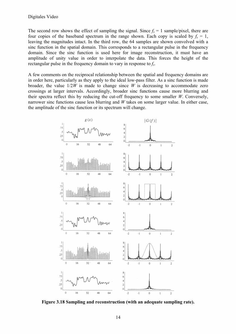
Examples of the concepts discussed in this chapter are concisely depicted in Figure 3.18, Figure 3.19, and Figure 3.20. They attempt to illustrate the effects of sampling and low-pass filtering on the quality of the reconstructed signal and its spectrum. The first row of Fig. 3.18 shows a signal and its spectra, bandlimited to .5 cycle/pixel. For pedagogical purposes, we treat this signal as if it is continuous. In actuality, though, it is really a 256-sample horizontal cross-section taken from the Mandrill image. Since each pixel has 4 samples contributing to it, there is a maximum of two cycles per pixel. The horizontal axes of the spectra account for this fact.

Digitales Video

14

The second row shows the effect of sampling the signal. Since fs = 1 sample/pixel, there are four copies of the baseband spectrum in the range shown. Each copy is scaled by fs = 1, leaving the magnitudes intact. In the third row, the 64 samples are shown convolved with a sinc function in the spatial domain. This corresponds to a rectangular pulse in the frequency domain. Since the sinc function is used here for image reconstruction, it must have an amplitude of unity value in order to interpolate the data. This forces the height of the rectangular pulse in the frequency domain to vary in response to fs.

A few comments on the reciprocal relationship between the spatial and frequency domains are in order here, particularly as they apply to the ideal low-pass filter. As a sinc function is made broader, the value 1/2W is made to change since W is decreasing to accommodate zero crossings at larger intervals. Accordingly, broader sinc functions cause more blurring and their spectra reflect this by reducing the cut-off frequency to some smaller W. Conversely, narrower sinc functions cause less blurring and W takes on some larger value. In either case, the amplitude of the sinc function or its spectrum will change.

Figure 3.18 Sampling and reconstruction (with an adequate sampling rate).

Digitales Video

15

That is, we can fix the amplitude of the sinc function so that only the rectangular pulse of the spectrum changes height A/2W as W varies. Alteratively, we can fix A/2W to remain constant as W changes, forcing us to vary A. The choice depends on the application.

When the sinc function is used to interpolate data, it is necessary to fix A to 1. Therefore, as the sampling density changes, the positions of the zero crossings shift, causing W to vary. This makes the amplitude of the spectrum's rectangular pulse change. On the other hand, if the sinc function is applied to bandlimit, not interpolate, the input signal, then it is important to fix A/2W to 1 so that the passband frequencies remain intact. Since W is once again varying, A must change proportionately to keep A/2W constant. Therefore, this application of the ideal low-pass filter requires the amplitude of the sinc function to be responsive to W.

In the examples presented below, our objective is to interpolate (reconstruct) the input and so A = 1 regardless of the sampling density. Consequently, the height of the spectrum of the reconstruction filter changes. To make the Fourier transforms of the filters easier to see, we have not drawn the frequency response of the reconstruction filters to scale. Therefore, the rectangular pulse function in the third row of Figure 3.18 actually has height A/2W = 1. The fourth row of the figure shows the result after applying the ideal low-pass filter. As sampling theory predicts, the output is identical to the original signal. The last two rows of the figure illustrate the consequences of nonideal reconstruction filtering. Instead of using a sinc function, a triangle function corresponding to linear interpolation was applied. In the frequency domain this corresponds to the square of the sinc function. Not surprisingly, the spectrum of the reconstructed signal suffers in both the passband and the stopband.

The identical sequence of filtering operations is performed in Figure 3.19. In this figure, though, the sampling rate has been lowered to fs = .5, meaning that only one sample is collected for every two output pixels. Consequently, the replicated spectra are multiplied by .5, leaving the magnitudes at 4. Unfortunately, this sampling rate causes the replicated spectra to overlap. This, in turn, gives rise to aliasing, as depicted in the fourth row of the figure. Applying the triangle function to perform linear interpolation also yields poor results.

In order to combat these artifacts, the input signal must be bandlimited to accommodate the low sampling rate. This is shown in the second row of Figure 3.20 where we see that all frequencies beyond W =.25 are truncated. This causes the input signal to be blurred. In this manner we have traded aliasing for blurring, a far less objectionable artifact. Sampling this function no longer causes the replicated copies to overlap. Convolving with an ideal low-pass filter now properly isolates the bandlimited spectrum.

Digitales Video

16

Figure 3.19 Sampling and reconstruction (with an inadequate sampling rate).

Digitales Video

17

Figure 3.20 Antialiasing filtering, sampling, and reconstruction stages.

References:

[1] George Wolberg. Digital Image Warping. IEEE Computer Society Press, Los Alamitos, CA, USA, 1994.