2.3.1. (a) cumulative class cumulative relative ... -...
TRANSCRIPT

Chapter 2 Exercise Solutions
1
Chapter 2 2.3.1. (a)
Cumulative Class Cumulative Relative relative
interval Frequency frequency frequency frequency 0-0.49 3 3 3.33 3.33 .5-0.99 3 6 3.33 6.67 1.0-1.49 15 21 16.67 23.33 1.5-1.99 15 36 16.67 40.0 2.0-2.49 45 81 50.0 90.00 2.5-2.99 9 90 10.0 100.0
pindex
Freq
uenc
y
2.752.251.751.250.750.25
50
40
30
20
10
0
Histogram of pindex
pindex
Freq
uenc
y
3.252.752.251.751.250.750.25
50
40
30
20
10
0
Frequency Polygon of pindex
Chapter 2 Exercise Solutions
2
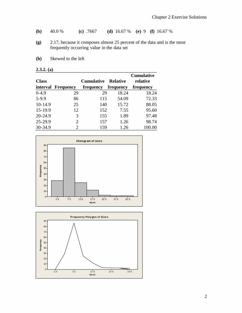
(b) 40.0 % (c) .7667 (d) 16.67 % (e) 9 (f) 16.67 % (g) 2.17, because it composes almost 25 percent of the data and is the most
frequently occurring value in the data set (h) Skewed to the left 2.3.2. (a) Cumulative Class Cumulative Relative relative interval Frequency frequency frequency frequency 0-4.9 29 29 18.24 18.24 5-9.9 86 115 54.09 72.33 10-14.9 25 140 15.72 88.05 15-19.9 12 152 7.55 95.60 20-24.9 3 155 1.89 97.48 25-29.9 2 157 1.26 98.74 30-34.9 2 159 1.26 100.00
sizes
Fre
qu
en
cy
32.527.522.517.512.57.52.5
90
80
70
60
50
40
30
20
10
0
Histogram of sizes
sizes
Fre
que
ncy
37.527.517.57.5-2.5
90
80
70
60
50
40
30
20
10
0
Frequency Polygon of Sizes
Chapter 2 Exercise Solutions
3
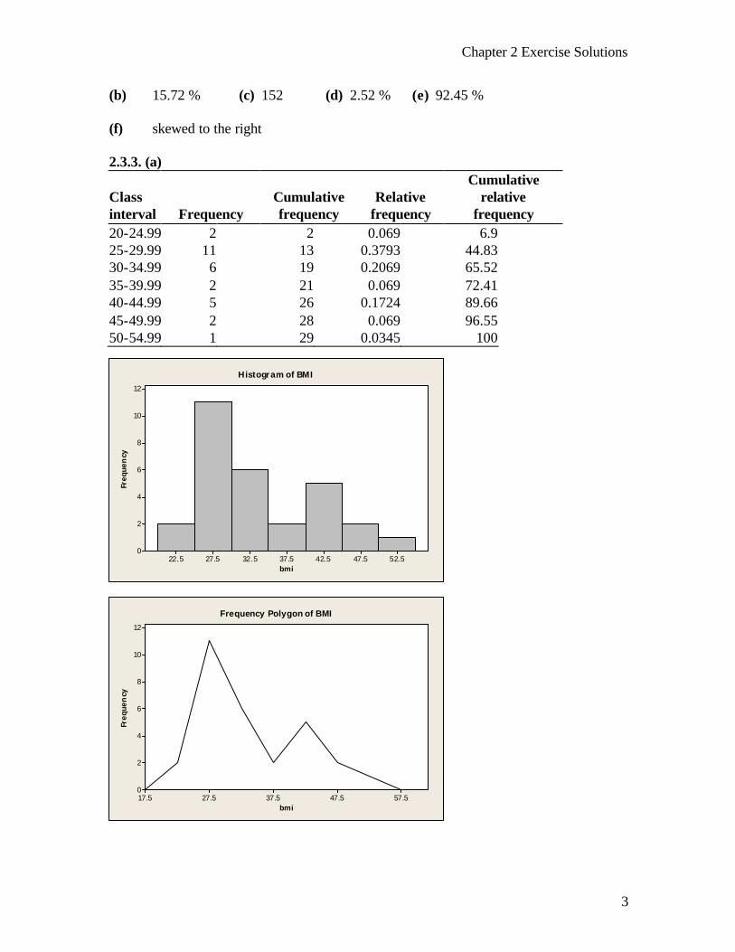
(b) 15.72 % (c) 152 (d) 2.52 % (e) 92.45 % (f) skewed to the right 2.3.3. (a) Cumulative Class Cumulative Relative relative interval Frequency frequency frequency frequency 20-24.99 2 2 0.069 6.9 25-29.99 11 13 0.3793 44.83 30-34.99 6 19 0.2069 65.52 35-39.99 2 21 0.069 72.41 40-44.99 5 26 0.1724 89.66 45-49.99 2 28 0.069 96.55 50-54.99 1 29 0.0345 100
bmi
Freq
uen
cy
52.547.542.537.532.527.522.5
12
10
8
6
4
2
0
Histogram of BMI
bmi
Freq
uen
cy
57.547.537.527.517.5
12
10
8
6
4
2
0
Frequency Polygon of BMI

Chapter 2 Exercise Solutions
4
(b) 44.83 % (c) 24.14 % (d) 34.48 % (e) Skewed to the right (f) 21 2.3.4. (a) Cumulative Class Cumulative Relative relative Interval Frequency frequency frequency frequency 5-9.99 1 1 1.89 1.89 10-14.99 3 4 5.66 7.55 15-19.99 6 10 11.32 18.87 20-24.99 7 17 13.21 32.08 25-29.99 12 29 22.64 54.72 30-34.99 11 40 20.75 75.47 35-39.99 7 47 13.21 88.68 40-44.99 2 49 3.77 92.45 45-49.99 2 51 3.77 96.23 50-54.99 0 51 0.00 96.23 55-59.99 2 53 3.77 100.00
Selevels
Fre
que
ncy
57.547.537.527.517.57.5
12
10
8
6
4
2
0
Histogram of Selevels
Selevels
Fre
que
ncy
62.552.542.532.522.512.52.5
12
10
8
6
4
2
0
Frequency Polygon of Selevels
Chapter 2 Exercise Solutions
5
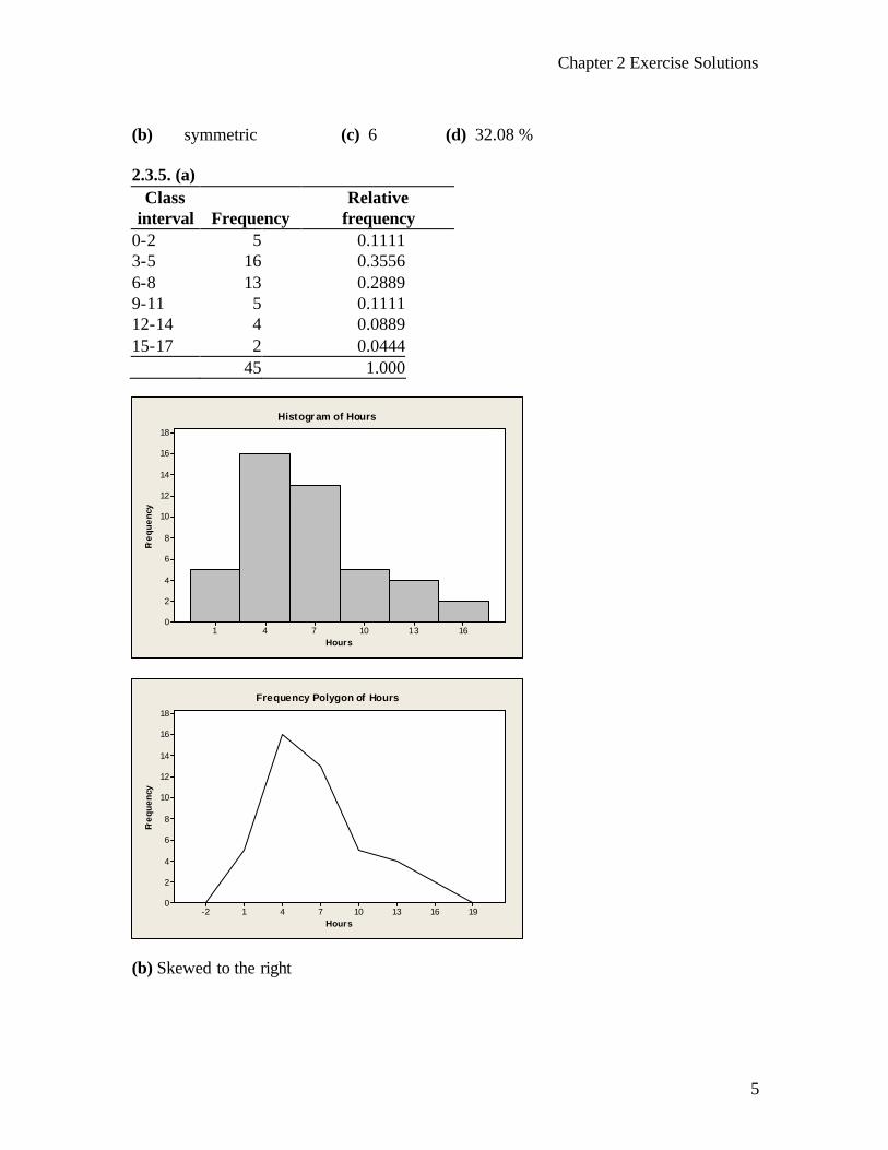
(b) symmetric (c) 6 (d) 32.08 % 2.3.5. (a)
Class Relative interval Frequency frequency
0-2 5 0.1111 3-5 16 0.3556 6-8 13 0.2889 9-11 5 0.1111 12-14 4 0.0889 15-17 2 0.0444 45 1.000
Hours
Fre
qu
en
cy
161310741
18
16
14
12
10
8
6
4
2
0
Histogram of Hours
Hours
Fre
qu
en
cy
19161310741-2
18
16
14
12
10
8
6
4
2
0
Frequency Polygon of Hours
(b) Skewed to the right
Chapter 2 Exercise Solutions
6
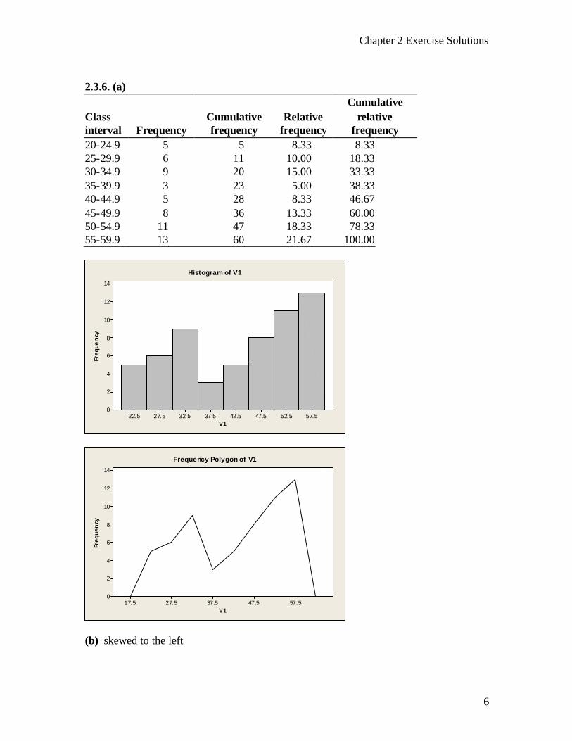
2.3.6. (a) Cumulative Class Cumulative Relative relative interval Frequency frequency frequency frequency 20-24.9 5 5 8.33 8.33 25-29.9 6 11 10.00 18.33 30-34.9 9 20 15.00 33.33 35-39.9 3 23 5.00 38.33 40-44.9 5 28 8.33 46.67 45-49.9 8 36 13.33 60.00 50-54.9 11 47 18.33 78.33 55-59.9 13 60 21.67 100.00
V1
Freq
uen
cy
57.552.547.542.537.532.527.522.5
14
12
10
8
6
4
2
0
Histogram of V1
V1
Freq
uen
cy
57.547.537.527.517.5
14
12
10
8
6
4
2
0
Frequency Polygon of V1
(b) skewed to the left
Chapter 2 Exercise Solutions
7
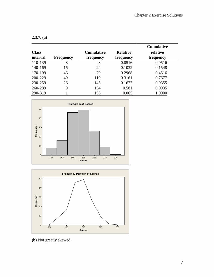
2.3.7. (a)
Cumulative Class Cumulative Relative relative interval Frequency frequency frequency frequency 110-139 8 8 0.0516 0.0516 140-169 16 24 0.1032 0.1548 170-199 46 70 0.2968 0.4516 200-229 49 119 0.3161 0.7677 230-259 26 145 0.1677 0.9355 260-289 9 154 0.581 0.9935 290-319 1 155 0.065 1.0000
Scores
Fre
quen
cy
305275245215185155125
50
40
30
20
10
0
Histogram of Scores
Scores
Freq
uen
cy
33527521515595
50
40
30
20
10
0
Frequency Polygon of Scores
(b) Not greatly skewed
Chapter 2 Exercise Solutions
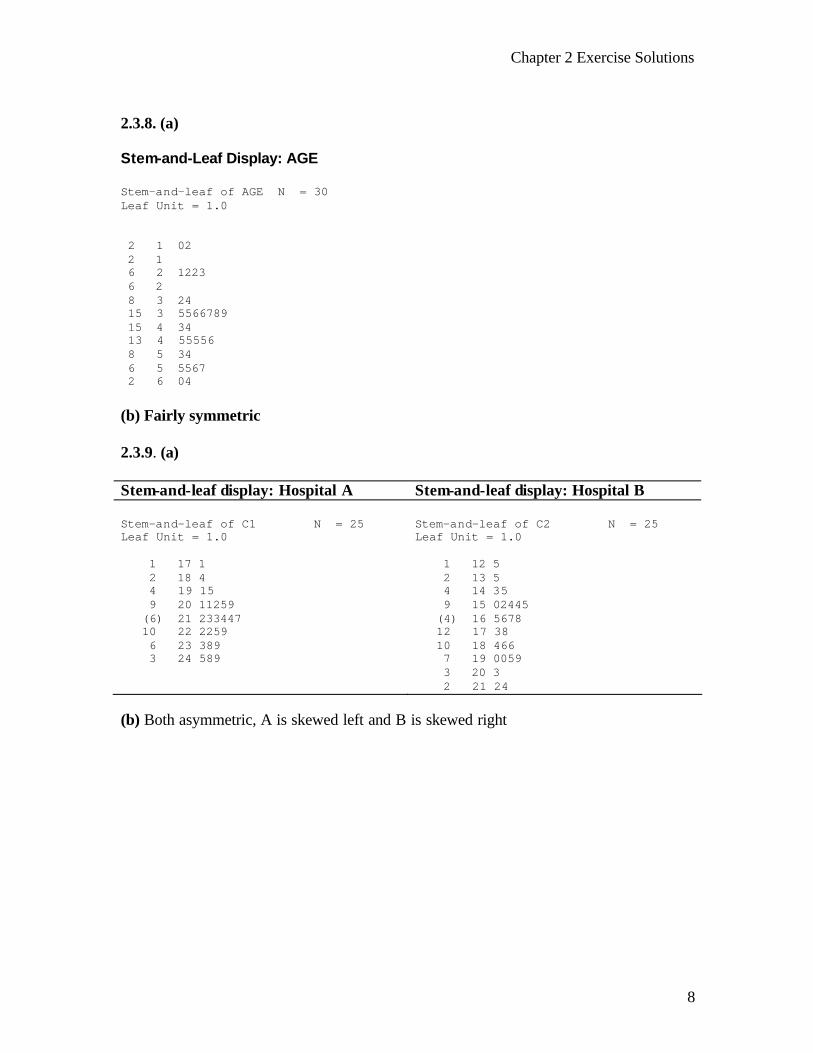
8
2.3.8. (a) Stem-and-Leaf Display: AGE Stem-and-leaf of AGE N = 30 Leaf Unit = 1.0 2 1 02 2 1 6 2 1223 6 2 8 3 24 15 3 5566789 15 4 34 13 4 55556 8 5 34 6 5 5567 2 6 04 (b) Fairly symmetric 2.3.9. (a) Stem-and-leaf display: Hospital A Stem-and-leaf display: Hospital B Stem-and-leaf of C1 N = 25 Leaf Unit = 1.0 1 17 1 2 18 4 4 19 15 9 20 11259 (6) 21 233447 10 22 2259 6 23 389 3 24 589
Stem-and-leaf of C2 N = 25 Leaf Unit = 1.0 1 12 5 2 13 5 4 14 35 9 15 02445 (4) 16 5678 12 17 38 10 18 466 7 19 0059 3 20 3 2 21 24
(b) Both asymmetric, A is skewed left and B is skewed right
Chapter 2 Exercise Solutions
9
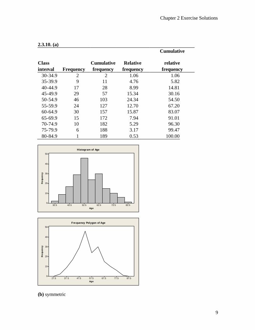
2.3.10. (a) Cumulative
Class
Cumulative Relative relative interval Frequency frequency frequency frequency
30-34.9 2 2 1.06 1.06 35-39.9 9 11 4.76 5.82 40-44.9 17 28 8.99 14.81 45-49.9 29 57 15.34 30.16 50-54.9 46 103 24.34 54.50 55-59.9 24 127 12.70 67.20 60-64.9 30 157 15.87 83.07 65-69.9 15 172 7.94 91.01 70-74.9 10 182 5.29 96.30 75-79.9 6 188 3.17 99.47 80-84.9 1 189 0.53 100.00
Age
Fre
quen
cy
82.572.562.552.542.532.5
50
40
30
20
10
0
Histogram of Age
Age
Fre
quen
cy
87.577.567.557.547.537.527.5
50
40
30
20
10
0
Frequency Polygon of Age
(b) symmetric
Chapter 2 Exercise Solutions
10
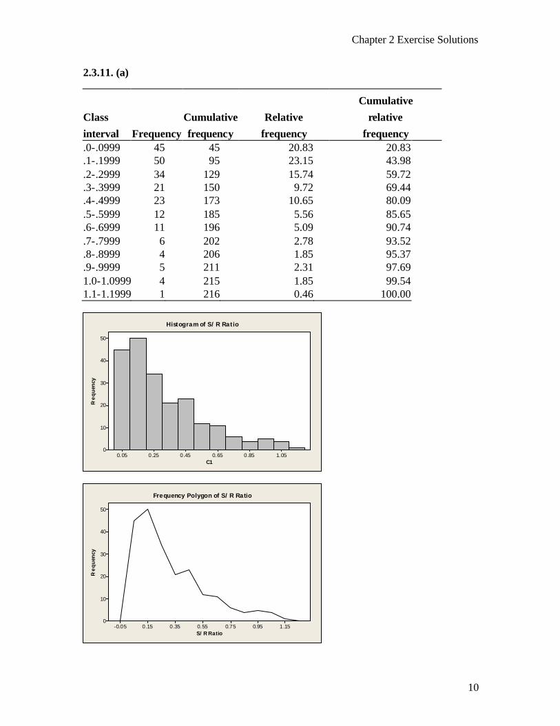
2.3.11. (a)
Cumulative Class Cumulative Relative relative interval Frequency frequency frequency frequency .0-.0999 45 45 20.83 20.83 .1-.1999 50 95 23.15 43.98 .2-.2999 34 129 15.74 59.72 .3-.3999 21 150 9.72 69.44 .4-.4999 23 173 10.65 80.09 .5-.5999 12 185 5.56 85.65 .6-.6999 11 196 5.09 90.74 .7-.7999 6 202 2.78 93.52 .8-.8999 4 206 1.85 95.37 .9-.9999 5 211 2.31 97.69 1.0-1.0999 4 215 1.85 99.54 1.1-1.1999 1 216 0.46 100.00
C1
Fre
qu
ency
1.050.850.650.450.250.05
50
40
30
20
10
0
Histogram of S/R Ratio
S/R Ratio
Fre
qu
ency
1.150.950.750.550.350.15-0.05
50
40
30
20
10
0
Frequency Polygon of S/R Ratio
Chapter 2 Exercise Solutions
11
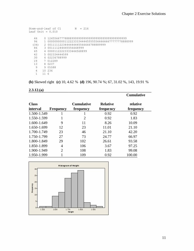
Stem-and-leaf of C1 N = 216 Leaf Unit = 0.010 46 0 1245566777888899999999999999999999999999999999 96 1 00000000001122233334444555555666666677777778888999 (34) 2 0011111223444444445566666788889999 86 3 001111244445556668999 65 4 00001122223333444568899 42 5 002334444599 30 6 02236788999 19 7 012289 13 8 0237 9 9 05588 4 10 236 1 11 6 (b) Skewed right (c) 10, 4.62 % (d) 196, 90.74 %; 67, 31.02 %, 143, 19.91 % 2.3.12.(a) Cumulative
Class
Cumulative Relative relative interval Frequency frequency frequency frequency 1.500-1.549 1 1 0.92 0.92 1.550-1.599 1 2 0.92 1.83 1.600-1.649 9 11 8.26 10.09 1.650-1.699 12 23 11.01 21.10 1.700-1.749 23 46 21.10 42.20 1.750-1.799 27 73 24.77 66.97 1.800-1.849 29 102 26.61 93.58 1.850-1.899 4 106 3.67 97.25 1.900-1.949 2 108 1.83 99.08 1.950-1.999 1 109 0.92 100.00
Height
Fre
que
ncy
1.9251.8251.7251.6251.525
30
25
20
15
10
5
0
Histogram of Height
Chapter 2 Exercise Solutions
12
Height
Fre
que
ncy
1.9751.8751.7751.6751.5751.475
30
25
20
15
10
5
0
Frequency Polygon of Height
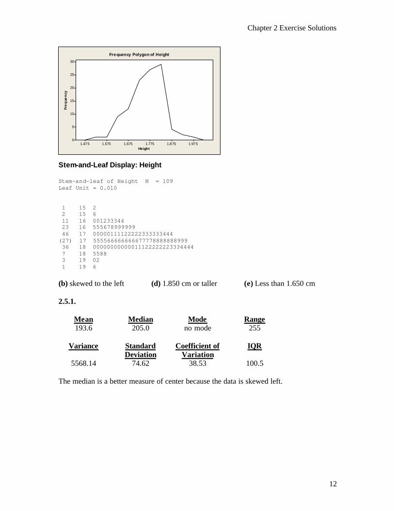
Stem-and-Leaf Display: Height Stem-and-leaf of Height N = 109 Leaf Unit = 0.010 1 15 2 2 15 6 11 16 001233344 23 16 555678999999 46 17 00000111122222333333444 (27) 17 555566666666677778888888999 36 18 00000000000011122222223334444 7 18 5588 3 19 02 1 19 6 (b) skewed to the left (d) 1.850 cm or taller (e) Less than 1.650 cm 2.5.1.
Mean Median Mode Range 193.6 205.0 no mode 255
Variance Standard
Deviation Coefficient of
Variation IQR
5568.14 74.62 38.53 100.5 The median is a better measure of center because the data is skewed left.
Chapter 2 Exercise Solutions
13
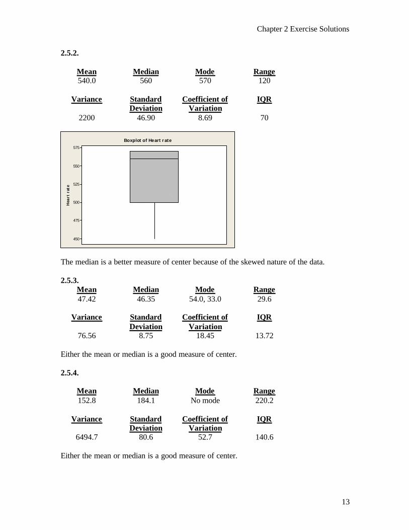
2.5.2.
Mean Median Mode Range 540.0 560 570 120
Variance Standard
Deviation Coefficient of
Variation IQR
2200 46.90 8.69 70
Hea
rt r
ate
575
550
525
500
475
450
Boxplot of Heart rate
The median is a better measure of center because of the skewed nature of the data. 2.5.3.
Mean Median Mode Range 47.42 46.35 54.0, 33.0 29.6
Variance Standard
Deviation Coefficient of
Variation IQR
76.56 8.75 18.45 13.72 Either the mean or median is a good measure of center. 2.5.4.
Mean Median Mode Range 152.8 184.1 No mode 220.2
Variance Standard
Deviation Coefficient of
Variation IQR
6494.7 80.6 52.7 140.6 Either the mean or median is a good measure of center.
Chapter 2 Exercise Solutions
14
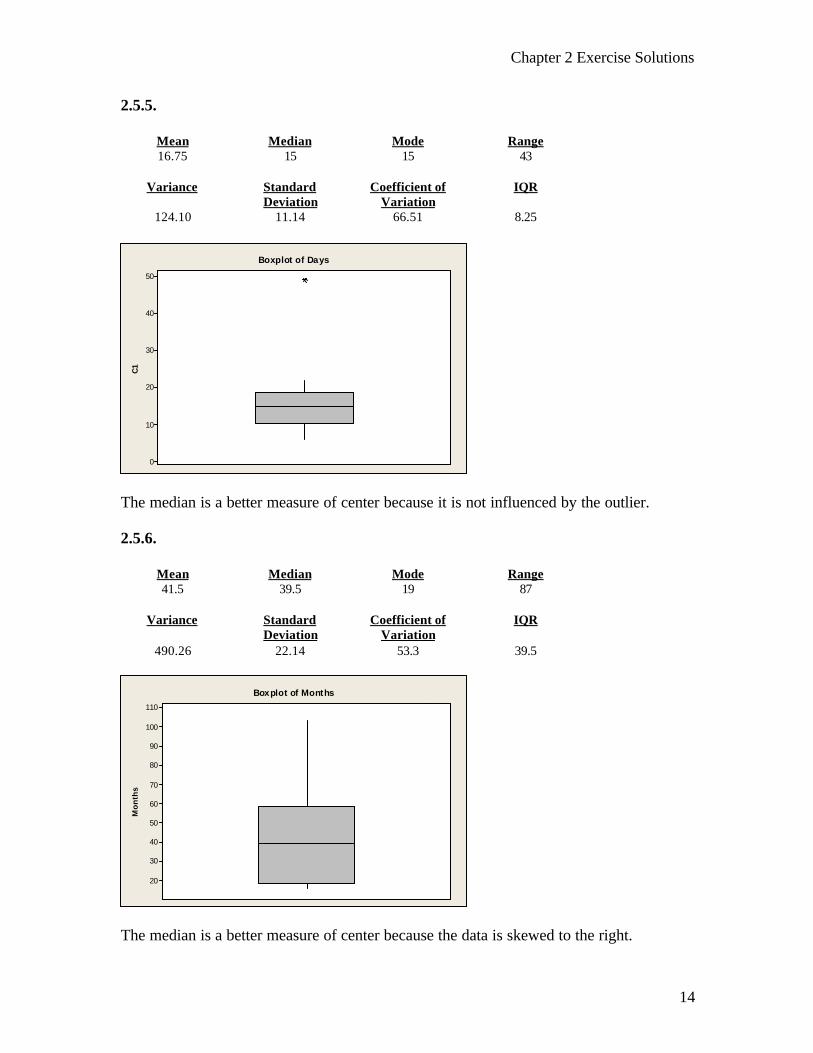
2.5.5.
Mean Median Mode Range 16.75 15 15 43
Variance Standard
Deviation Coefficient of
Variation IQR
124.10 11.14 66.51 8.25
C1
50
40
30
20
10
0
Boxplot of Days
The median is a better measure of center because it is not influenced by the outlier. 2.5.6.
Mean Median Mode Range 41.5 39.5 19 87
Variance Standard
Deviation Coefficient of
Variation IQR
490.26 22.14 53.3 39.5
Mo
nth
s
110
100
90
80
70
60
50
40
30
20
Boxplot of Months
The median is a better measure of center because the data is skewed to the right.
Chapter 2 Exercise Solutions
15
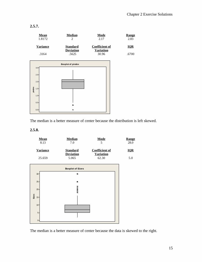
2.5.7.
Mean Median Mode Range 1.8172 2 2.17 2.83
Variance Standard
Deviation Coefficient of
Variation IQR
.3164 .5625 30.96 .6700
pind
ex
3.0
2.5
2.0
1.5
1.0
0.5
0.0
Boxplot of pindex
The median is a better measure of center because the distribution is left skewed. 2.5.8.
Mean Median Mode Range 8.13 7.0 5 28.0
Variance Standard
Deviation Coefficient of
Variation IQR
25.659 5.065 62.30 5.0
Siz
es
30
25
20
15
10
5
0
Boxplot of Sizes
The median is a better measure of center because the data is skewed to the right.

Chapter 2 Exercise Solutions
16
2.5.9.
Mean Median Mode Range 33.87 30.49 none 29.84
Variance Standard
Deviation Coefficient of
Variation IQR
64.00 8.00 23.62 13.4
bmi
55
50
45
40
35
30
25
Boxplot of BMI
The median is a better measure of center because the distribution is right skewed. 2.5.10.
Mean Median Mode Range 29.08 28.94 None 46.92
Variance Standard
Deviation Coefficient of
Variation IQR
107.68 10.38 35.68 12.94 The mean or the median is a good measure of center.
Chapter 2 Exercise Solutions
17
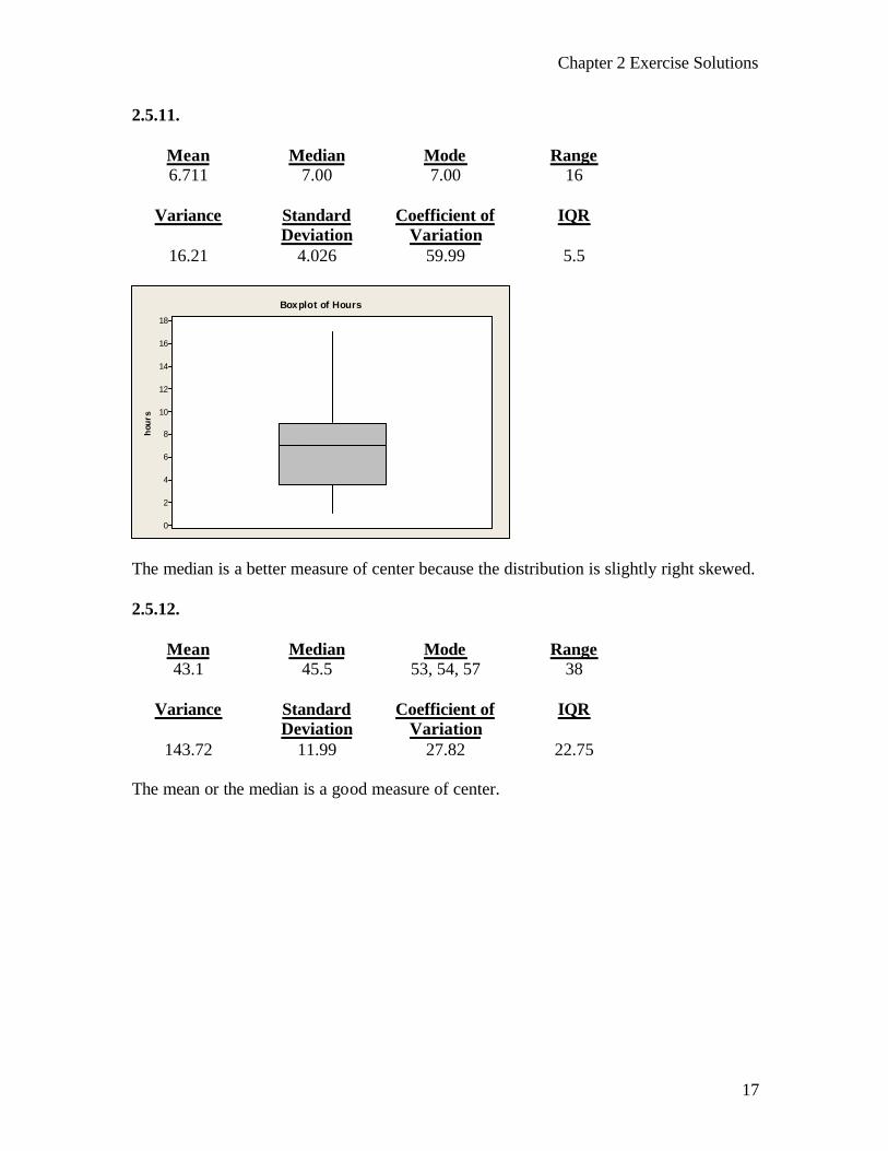
2.5.11.
Mean Median Mode Range 6.711 7.00 7.00 16
Variance Standard
Deviation Coefficient of
Variation IQR
16.21 4.026 59.99 5.5
hou
rs
18
16
14
12
10
8
6
4
2
0
Boxplot of Hours
The median is a better measure of center because the distribution is slightly right skewed. 2.5.12.
Mean Median Mode Range 43.1 45.5 53, 54, 57 38
Variance Standard
Deviation Coefficient of
Variation IQR
143.72 11.99 27.82 22.75 The mean or the median is a good measure of center.

Chapter 2 Exercise Solutions
18
2.5.13.
Mean Median Mode Range 204.19 204 212, 198 196
Variance Standard
Deviation Coefficient of
Variation IQR
1258.12 35.47 17.37 46
Sco
res
300
250
200
150
100
Boxplot of Scores
Either the mean or median is a good measure of center. 2.5.14.
Mean Median Mode Range 43.71 45 32, 48, 51 21.0
Variance Standard
Deviation Coefficient of
Variation IQR
48.07 6.93 15.86 11.75 The mean or the median is a good measure of center.
Chapter 2 Exercise Solutions
19
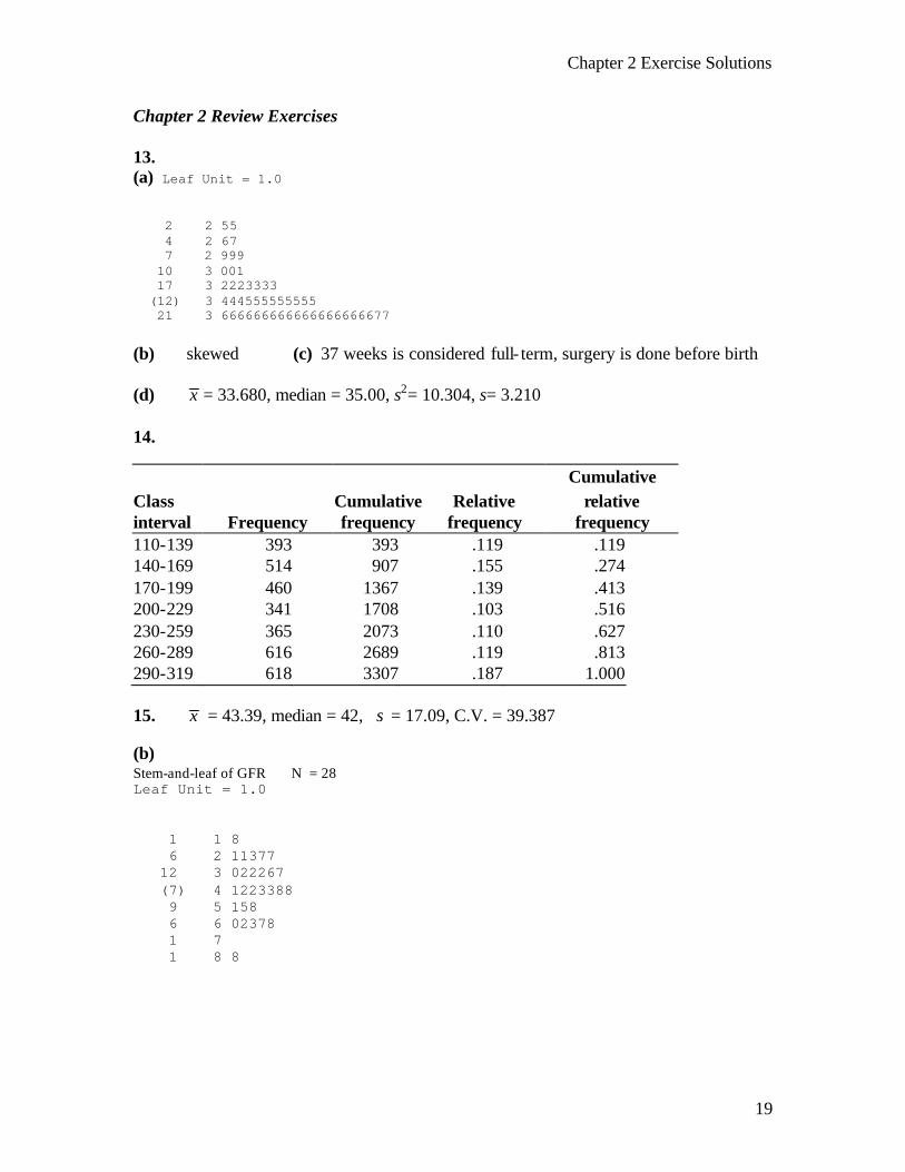
Chapter 2 Review Exercises 13. (a) Leaf Unit = 1.0 2 2 55 4 2 67 7 2 999 10 3 001 17 3 2223333 (12) 3 444555555555 21 3 666666666666666666677 (b) skewed (c) 37 weeks is considered full- term, surgery is done before birth (d) x = 33.680, median = 35.00, s2= 10.304, s= 3.210 14.
Cumulative Class Cumulative Relative relative interval Frequency frequency frequency frequency 110-139 393 393 .119 .119 140-169 514 907 .155 .274 170-199 460 1367 .139 .413 200-229 341 1708 .103 .516 230-259 365 2073 .110 .627 260-289 616 2689 .119 .813 290-319 618 3307 .187 1.000 15. x = 43.39, median = 42, s = 17.09, C.V. = 39.387 (b) Stem-and-leaf of GFR N = 28 Leaf Unit = 1.0 1 1 8 6 2 11377 12 3 022267 (7) 4 1223388 9 5 158 6 6 02378 1 7 1 8 8
Chapter 2 Exercise Solutions
20
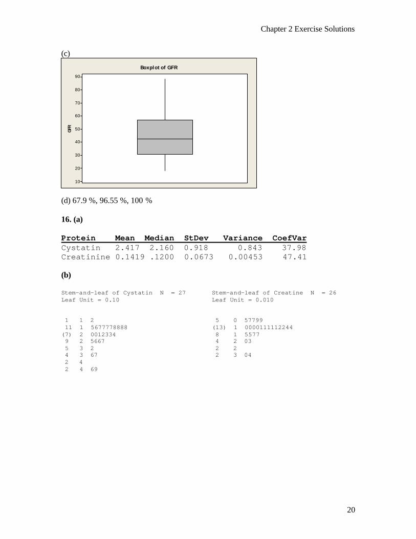
(c)
GFR
90
80
70
60
50
40
30
20
10
Boxplot of GFR
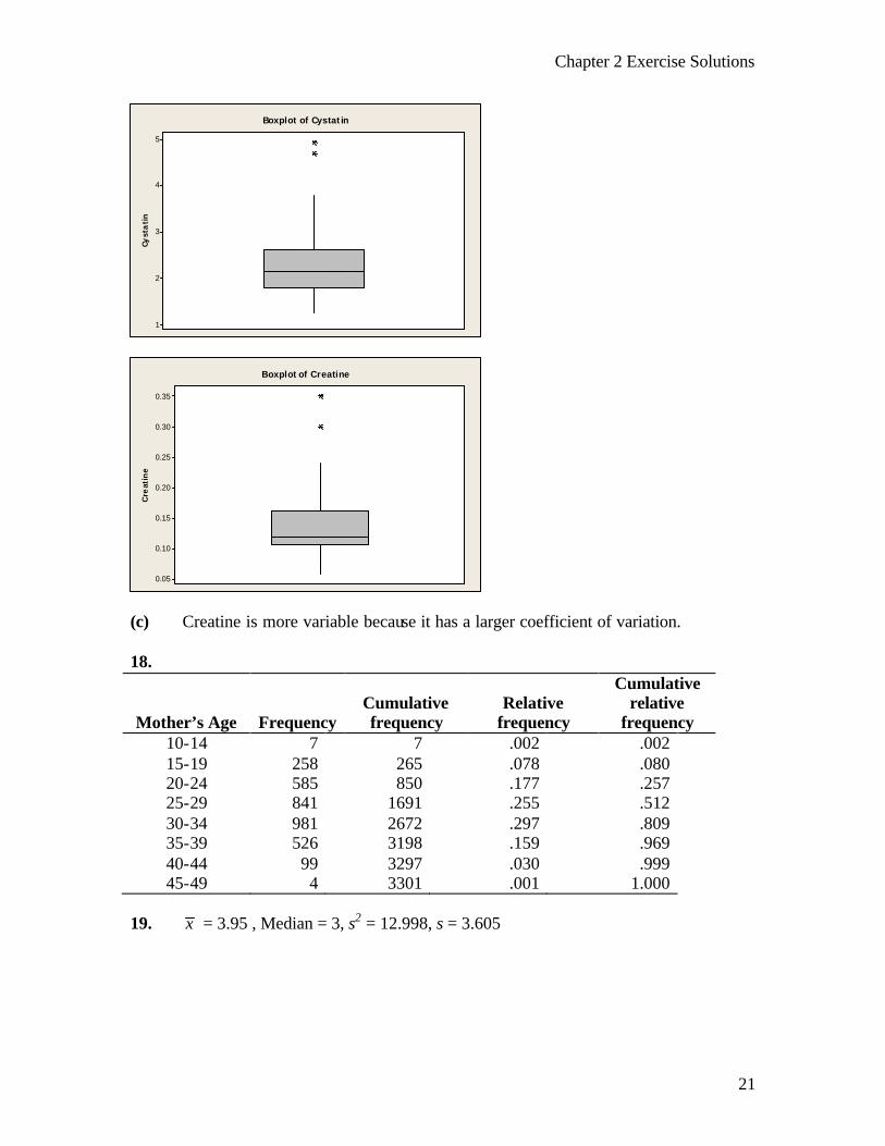
(d) 67.9 %, 96.55 %, 100 % 16. (a) Protein Mean Median StDev Variance CoefVar Cystatin 2.417 2.160 0.918 0.843 37.98 Creatinine 0.1419 .1200 0.0673 0.00453 47.41 (b) Stem-and-leaf of Cystatin N = 27 Leaf Unit = 0.10 1 1 2 11 1 5677778888 (7) 2 0012334 9 2 5667 5 3 2 4 3 67 2 4 2 4 69
Stem-and-leaf of Creatine N = 26 Leaf Unit = 0.010 5 0 57799 (13) 1 0000111112244 8 1 5577 4 2 03 2 2 2 3 04
Chapter 2 Exercise Solutions
21
Cyst
ati
n5
4
3
2
1
Boxplot of Cystatin
Cre
atin
e
0.35
0.30
0.25
0.20
0.15
0.10
0.05
Boxplot of Creatine
(c) Creatine is more variable because it has a larger coefficient of variation. 18.
Mother’s Age Frequency Cumulative frequency
Relative frequency
Cumulative relative
frequency 10-14 7 7 .002 .002 15-19 258 265 .078 .080 20-24 585 850 .177 .257 25-29 841 1691 .255 .512 30-34 981 2672 .297 .809 35-39 526 3198 .159 .969 40-44 99 3297 .030 .999 45-49 4 3301 .001 1.000
19. x = 3.95 , Median = 3, s2 = 12.998, s = 3.605
Chapter 2 Exercise Solutions
22
20. (a) The sum of the squared deviations of a set of measurements about their mean is smaller than any other sum of squared deviations about any other point.
(b) The sum of a set of measurements is equal to the product of their mean and the number of measurements.
(c) The sum of the deviations of a set of measurements about their mean is equal to
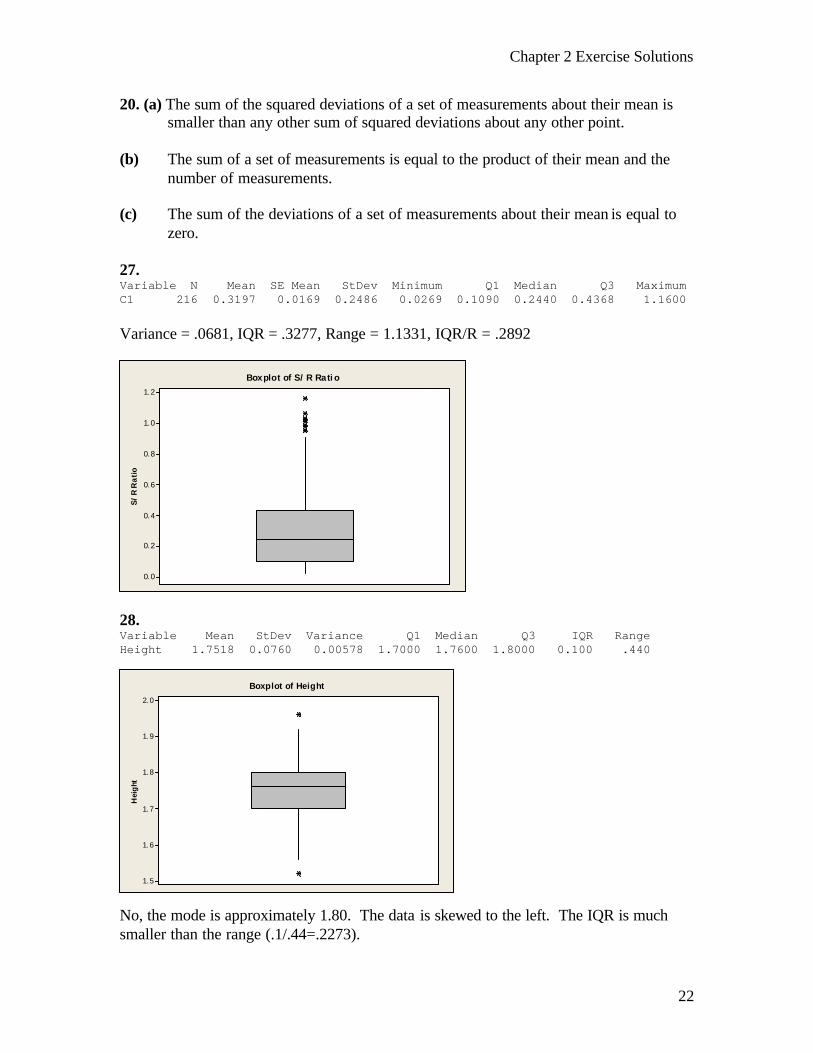
zero. 27. Variable N Mean SE Mean StDev Minimum Q1 Median Q3 Maximum C1 216 0.3197 0.0169 0.2486 0.0269 0.1090 0.2440 0.4368 1.1600 Variance = .0681, IQR = .3277, Range = 1.1331, IQR/R = .2892
S/
R R
ati
o
1.2
1.0
0.8
0.6
0.4
0.2
0.0
Boxplot of S/R Ratio
28. Variable Mean StDev Variance Q1 Median Q3 IQR Range Height 1.7518 0.0760 0.00578 1.7000 1.7600 1.8000 0.100 .440
Hei
ght
2.0
1.9
1.8
1.7
1.6
1.5
Boxplot of Height
No, the mode is approximately 1.80. The data is skewed to the left. The IQR is much smaller than the range (.1/.44=.2273).
Chapter 2 Exercise Solutions
23
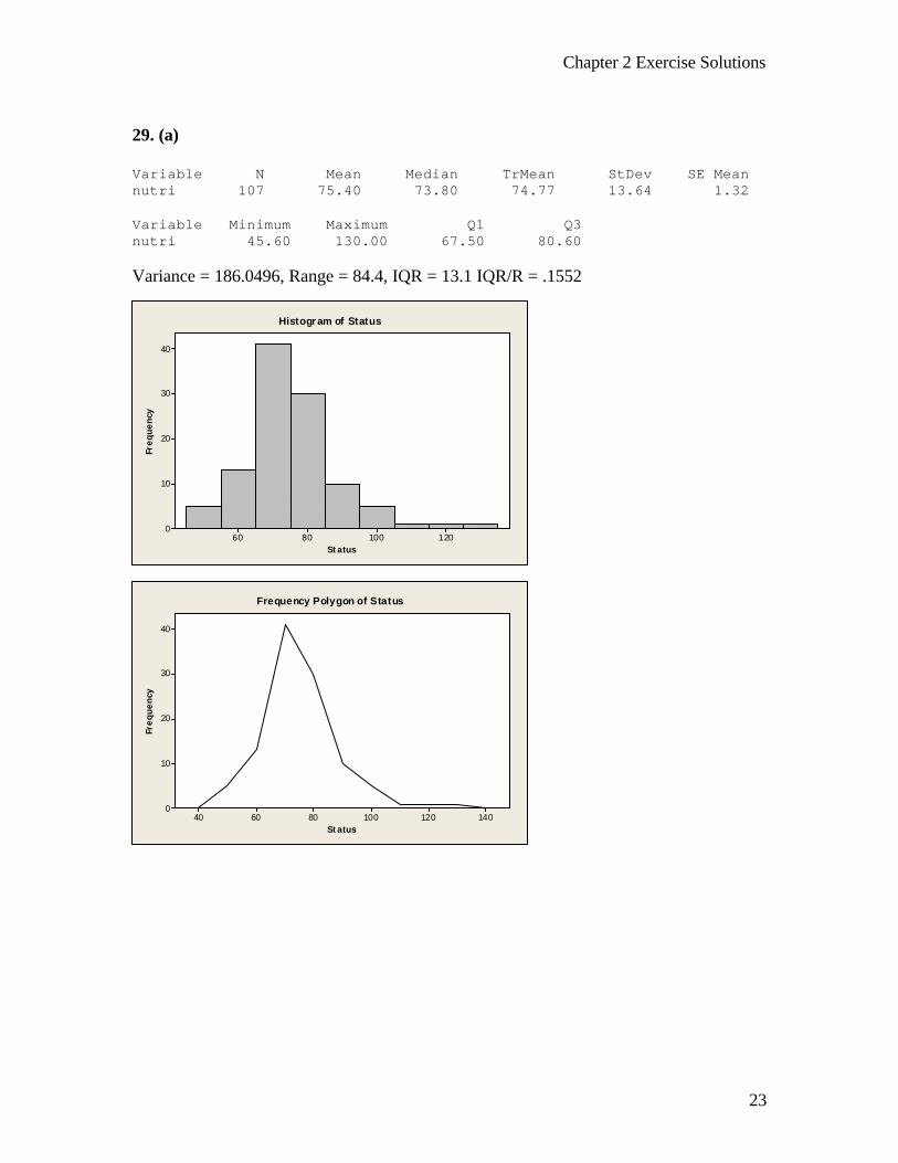
29. (a) Variable N Mean Median TrMean StDev SE Mean nutri 107 75.40 73.80 74.77 13.64 1.32 Variable Minimum Maximum Q1 Q3 nutri 45.60 130.00 67.50 80.60 Variance = 186.0496, Range = 84.4, IQR = 13.1 IQR/R = .1552
Status
Fre
qu
en
cy
1201008060
40
30
20
10
0
Histogram of Status
Status
Fre
qu
en
cy
140120100806040
40
30
20
10
0
Frequency Polygon of Status
Chapter 2 Exercise Solutions
24
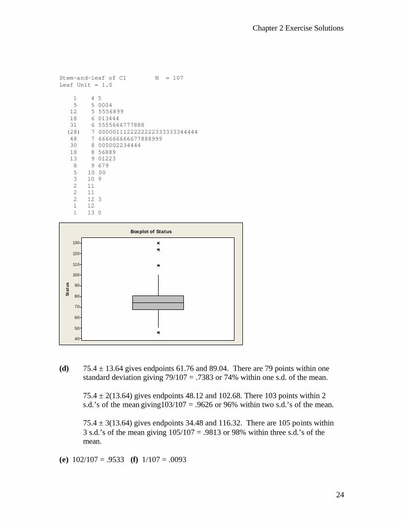
Stem-and-leaf of C1 N = 107 Leaf Unit = 1.0 1 4 5 5 5 0004 12 5 5556899 18 6 013444 31 6 5555666777888 (28) 7 0000011122222222333333344444 48 7 666666666677888999 30 8 000002234444 18 8 56889 13 9 01223 8 9 679 5 10 00 3 10 9 2 11 2 11 2 12 3 1 12 1 13 0
Stat
us
130
120
110
100
90
80
70
60
50
40
Boxplot of Status
(d) 75.4 ± 13.64 gives endpoints 61.76 and 89.04. There are 79 points within one
standard deviation giving 79/107 = .7383 or 74% within one s.d. of the mean.
75.4 ± 2(13.64) gives endpoints 48.12 and 102.68. There 103 points within 2 s.d.’s of the mean giving103/107 = .9626 or 96% within two s.d.’s of the mean. 75.4 ± 3(13.64) gives endpoints 34.48 and 116.32. There are 105 points within 3 s.d.’s of the mean giving 105/107 = .9813 or 98% within three s.d.’s of the mean.
(e) 102/107 = .9533 (f) 1/107 = .0093
Chapter 3 Exercise Solutions
25
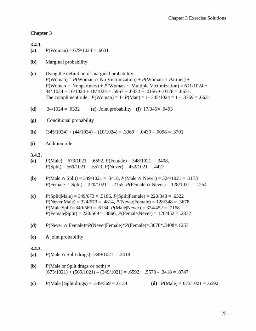
Chapter 3 3.4.1. (a) P(Woman) = 679/1024 = .6631 (b) Marginal probability (c) Using the definition of marginal probability:
P(Woman) = P(Woman ∩ No Victimization) + P(Woman ∩ Partner) + P(Woman ∩ Nonpartners) + P(Woman ∩ Multiple Victimization) = 611/1024 + 34/ 1024 + 16/1024 + 18/1024 = .5967 + .0332 + .0156 + .0176 = .6631. The compliment rule: P(Woman) = 1- P(Man) = 1- 345/1024 = 1 - .3369 = .6631
(d) 34/1024 = .0332 (e) Joint probability (f) 17/345= .0493 (g) Conditional probability (h) (345/1024) + (44/1024) – (10/1024) = .3369 + .0430 - .0098 = .3701 (i) Addition rule 3.4.2. (a) P(Male) = 673/1021 = .6592, P(Female) = 348/1021 = .3408, P(Split) = 569/1021 = .5573, P(Never) = 452/1021 = .4427 (b) P(Male ∩ Split) = 349/1021 = .3418, P(Male ∩ Never) = 324/1021 = .3173
P(Female ∩ Split) = 220/1021 = .2155, P(Female ∩ Never) = 128/1021 = .1254 (c) P(Split|Male) = 349/673 = .5186, P(Split|Female) = 220/348 = .6322 P(Never|Male) = 324/673 = .4814, P(Never|Female) = 128/348 = .3678 P(Male|Split)=349/569 = .6134, P(Male|Never) = 324/452 = .7168 P(Female|Split) = 220/569 = .3866, P(Female|Never) = 128/452 = .2832 (d) P(Never ∩ Female)=P(Never|Female)*P(Female)=.3678*.3408=.1253 (e) A joint probability 3.4.3. (a) P(Male ∩ Split drugs)= 349/1021 = .3418 (b) P(Male or Split drugs or both) =
(673/1021) + (569/1021) – (349/1021) = .6592 + .5573 - .3418 = .8747 (c) P(Male | Split drugs) = 349/569 = .6134 (d) P(Male) = 673/1021 = .6592
Chapter 3 Exercise Solutions
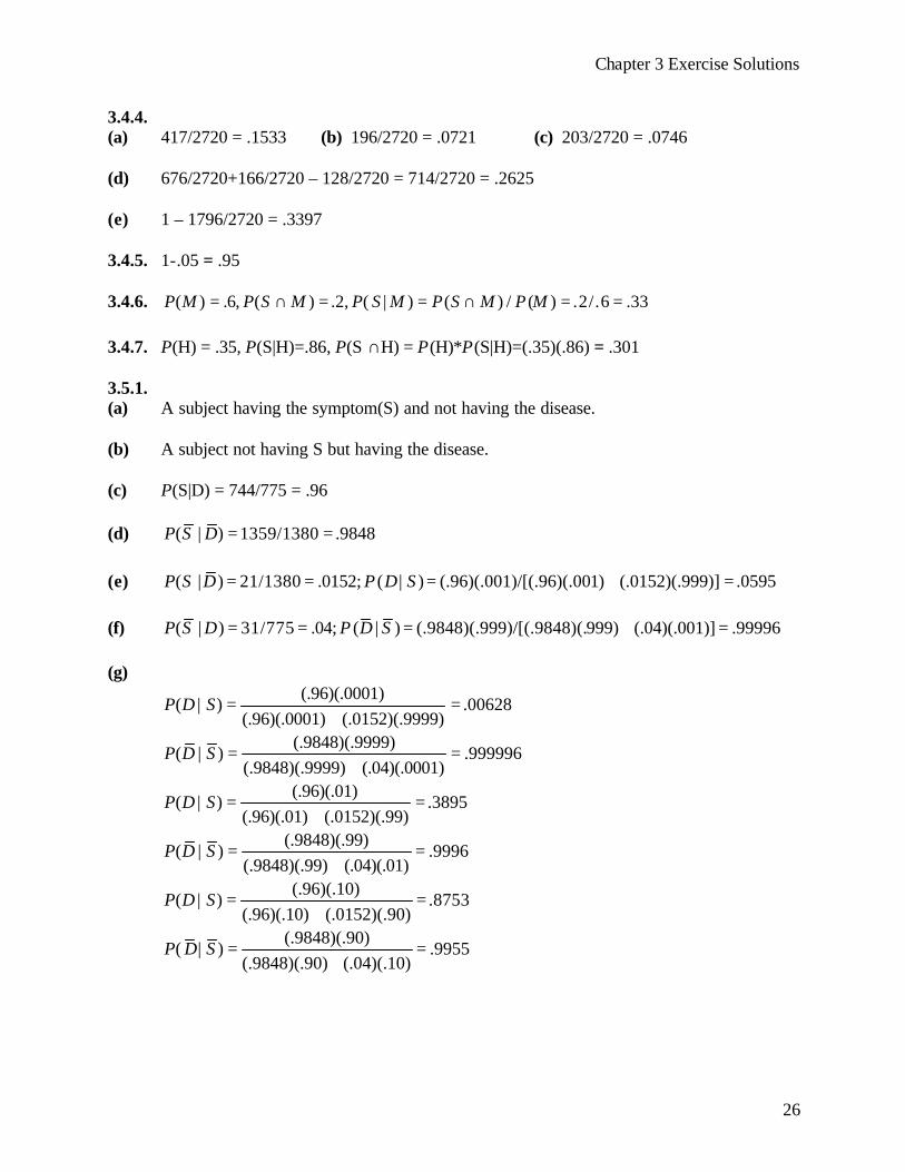
26
3.4.4. (a) 417/2720 = .1533 (b) 196/2720 = .0721 (c) 203/2720 = .0746 (d) 676/2720+166/2720 – 128/2720 = 714/2720 = .2625 (e) 1 – 1796/2720 = .3397 3.4.5. 1-.05 = .95 3.4.6. ( ) .6, ( ) .2, ( | ) ( ) / ( ) .2/.6 .33P M P S M P S M P S M P M= ∩ = = ∩ = = 3.4.7. P(H) = .35, P(S|H)=.86, P(S ∩H) = P(H)*P(S|H)=(.35)(.86) = .301 3.5.1. (a) A subject having the symptom(S) and not having the disease. (b) A subject not having S but having the disease. (c) P(S|D) = 744/775 = .96 (d) ( | ) 1359/1380 .9848P S D = = (e) ( | ) 21/1380 .0152; ( | ) (.96)(.001)/[(.96)(.001) (.0152)(.999)] .0595P S D P D S= = = + = (f) ( | ) 31/775 .04; ( | ) (.9848)(.999)/[(.9848)(.999) (.04)(.001)] .99996P S D P D S= = = + = (g)
(.96)(.0001)( | ) .00628
(.96)(.0001) (.0152)(.9999)P D S = =
+
(.9848)(.9999)( | ) .999996
(.9848)(.9999) (.04)(.0001)P D S = =
+
(.96)(.01)( | ) .3895
(.96)(.01) (.0152)(.99)P D S = =
+
(.9848)(.99)( | ) .9996
(.9848)(.99) (.04)(.01)P D S = =
+
(.96)(.10)( | ) .8753
(.96)(.10) (.0152)(.90)P D S = =
+
(.9848)(.90)( | ) .9955
(.9848)(.90) (.04)(.10)P D S = =
+

Chapter 3 Exercise Solutions
27
3.5.2 (a) Sensitivity = ( | ) 38/43 .8837;P T D = = (b) Specificity = ( | ) 18/28 .6429P T D = = (c) Probability of bucket-handle tears 3.5.3. Sensitivity = ( | ) .927;P T D = Specificity = ( | ) .997P T D = ;
( ) 1/320000 .00003125P D = = ; ( ) 1 .00003125 .99996875P D = − = ( | ) 1 ( | ) 1 .927 .073P T D P T D= − = − =
Predictive Value Negative = (.997)(.99996875)
.99999977(.997)(.99996875) (.073)(.00003125)
=+
Chapter 3 Review Exercises 3. (a) 459/2142 = .2143 (b) 319/578 = .5519 (c) 329/2142 = .1536 (d) 578/2142 + 490/2142 – 88/2142 = .2698 + .2288 – .0411 = .4575 (e) 1 - (1057/2142) = .5065 4. (a) 1. 29/56 = .517 2. 27/56 = .4821 3. 12/56 = .2143 4. (27+27-12)/56=42/56 = .75 5. 15/29 = .5172 (b) 1. True. Each is the probability of the joint occurrence of competent and enrolled in a CPR
course. 2. True. Each is the probability of the occurrence of competent or enrolled in a CPR course,
or both. 3. True. The marginal probability of A is equal to the sum of the joint probabilities of A
with each category of competence. 4. False. The addition rule is required. Should be ( ) ( ) ( ) ( )P B C P B P C P B C∪ = + − ∩ . 5. False. Training course and competence are not independent. 6. False. Training course and competence are not independent. 7. True. The training groups are mutually exclusive.
Chapter 3 Exercise Solutions
28
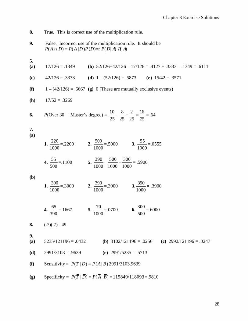
8. True. This is correct use of the multiplication rule. 9. False. Incorrect use of the multiplication rule. It should be
( ) ( | ) ( )or ( | ) ( )P A D P A D P D P D A P A∩ = 5. (a) 17/126 = .1349 (b) 52/126+42/126 – 17/126 = .4127 + .3333 – .1349 = .6111 (c) 42/126 = .3333 (d) 1 – (52/126) = .5873 (e) 15/42 = .3571 (f) 1 – (42/126) = .6667 (g) 0 (These are mutually exclusive events) (h) 17/52 = .3269
6. P(Over 30 ∪ Master’s degree) = 10 8 2 16
.6425 25 25 25
+ − = =
7. (a)
1. 220
1000=.2200 2.
5001000
=.5000 3. 55
1000=.0555
4. 55
500=.1100 5.
390 500 3001000 1000 1000
+ − = .5900
(b)
1. 300
1000=.3000 2.
3901000
=.3900 3.390
1000= .3900
4. 65
390=.1667 5.
701000
=.0700 6. 300500
=.6000
8. (.7)(.7)=.49 9. (a) 5235/121196 = .0432 (b) 3102/121196 = .0256 (c) 2992/121196 = .0247 (d) 2991/3103 = .9639 (e) 2991/5235 = .5713 (f) Sensitivity = ( | ) ( | )P T D P A B= 2991/3103.9639 (g) Specificity = ( | ) ( | ) 115849/118093P T D P A B= = =.9810
Chapter 3 Exercise Solutions
29
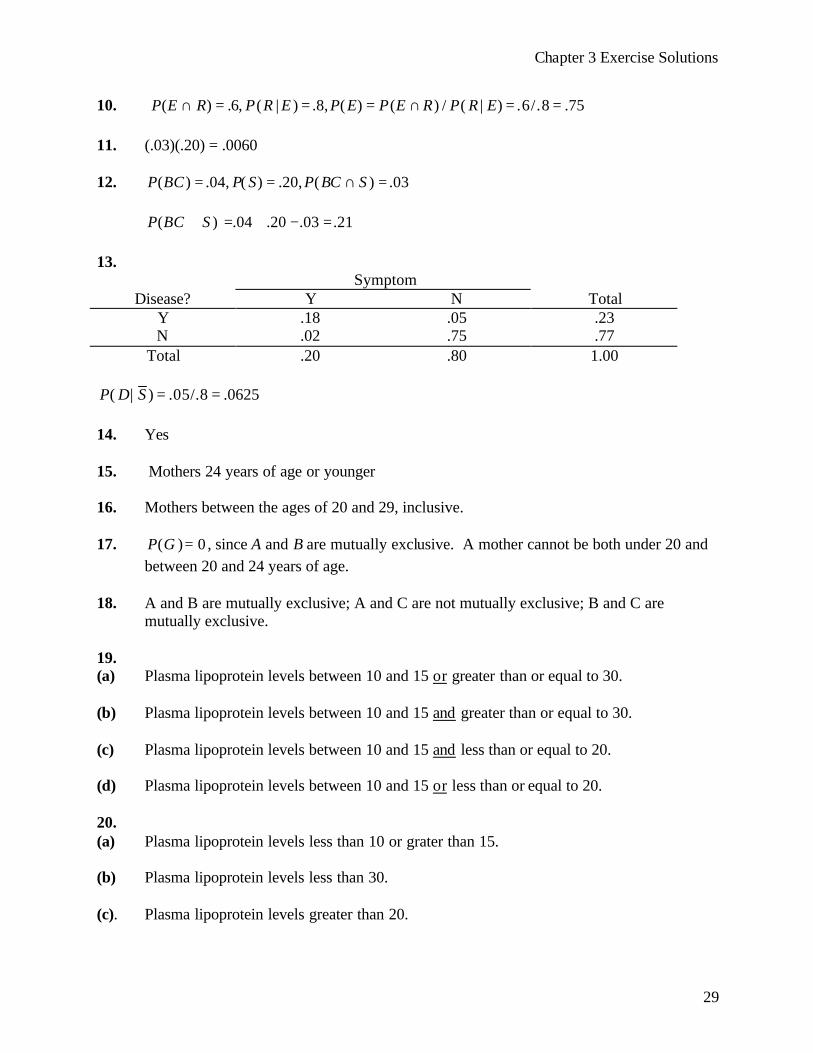
10. ( ) .6, ( | ) .8, ( ) ( ) / ( | ) .6/.8 .75P E R P R E P E P E R P R E∩ = = = ∩ = = 11. (.03)(.20) = .0060 12. ( ) .04, ( ) .20, ( ) .03P BC P S P BC S= = ∩ =
( ) .04 .20 .03 .21P BC S∪ = + − = 13.
Symptom Disease? Y N Total
Y .18 .05 .23 N .02 .75 .77
Total .20 .80 1.00
( | ) .05/.8P D S = = .0625 14. Yes 15. Mothers 24 years of age or younger 16. Mothers between the ages of 20 and 29, inclusive. 17. ( ) 0P G = , since A and B are mutually exclusive. A mother cannot be both under 20 and
between 20 and 24 years of age. 18. A and B are mutually exclusive; A and C are not mutually exclusive; B and C are
mutually exclusive. 19. (a) Plasma lipoprotein levels between 10 and 15 or greater than or equal to 30. (b) Plasma lipoprotein levels between 10 and 15 and greater than or equal to 30. (c) Plasma lipoprotein levels between 10 and 15 and less than or equal to 20. (d) Plasma lipoprotein levels between 10 and 15 or less than or equal to 20. 20. (a) Plasma lipoprotein levels less than 10 or grater than 15. (b) Plasma lipoprotein levels less than 30. (c). Plasma lipoprotein levels greater than 20.
Chapter 3 Exercise Solutions
30
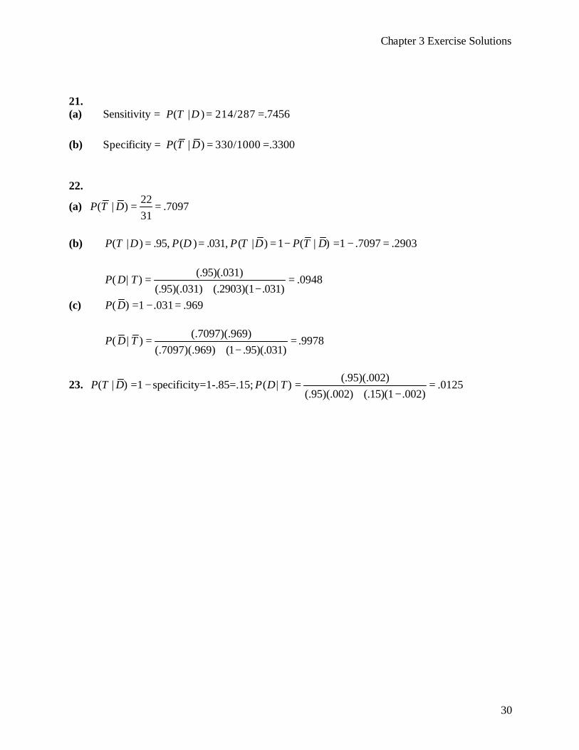
21. (a) Sensitivity = ( | ) 214/287P T D = =.7456 (b) Specificity = ( | ) 330/1000P T D = =.3300 22.
(a) 22
( | ) .709731
P T D = =
(b) ( | ) .95, ( ) .031, ( | ) 1 ( | ) 1 .7097 .2903P T D P D P T D P T D= = = − = − =
(.95)(.031)
( | ) .0948(.95)(.031) (.2903)(1 .031)
P D T = =+ −
(c) ( ) 1 .031 .969P D = − =
(.7097)(.969)
( | ) .9978(.7097)(.969) (1 .95)(.031)
P D T = =+ −
23. (.95)(.002)
( | ) 1 specificity=1-.85=.15; ( | )(.95)(.002) (.15)(1 .002)
P T D P D T= − = =+ −
.0125
Chapter 4 Exercise Solutions
31
Chapter 4 4.3.1. (a) 17 3
20 3(.76) (.24)C = .1484 (b) 20 0 19 1 18 2
20 0 20 1 20 21 (.76) (.24) (.76) (.24) (.76) (.24)C C C − + + =
1 [.0041 .0261 .0783] .8915− + + = (c) 20 0 19 1 18 2
20 0 20 1 20 2(.76) (.24) (.76) (.24) (.76) (.24) .0041 .0261 .0783C C C+ + = + + = .1085
(d) 17 3 16 4
20 3 20 4(.76) (.24) (.76) (.24)C C+ +
15 5 14 6 13 720 5 20 6 20 7(.76) (.24) (.76) (.24) (.76) (.24)C C C+ + = .1484 .1991 .2012 .1589 .1003 .8079+ + + + =
4.3.2. np = 20(.24) = 4.80 4.3.3. (a) 5 0
5 0(.76) (.24) .2536C =
(b) 3 2 2 3 1 4 0 5
5 2 5 3 5 4 5 5(.76) (.24) (.76) (.24) (.76)(.24) (.76) (.24)
.2529 .0798 .0126 .0008 .3461
C C C C+ + + =
+ + + =
(c) 4 1 3 2 2 3
5 1 5 2 5 3(.76) (.24) (.76) (.24) (.76) (.24)
.4003 .2529 .0798 .7330
C C C+ + =
+ + =
(d) 5 0 4 1 3 2
5 0 5 1 5 2(.76) (.24) (.76) (.24) (.76) (.24)
.2536 .4003 .2529 .9068
C C C+ + =
+ + =
(e) 0 5
5 5(.76) (.24) .0008C = 4.3.4. (a) 12 3
15 3.68 .32 .1457C = (b) .5187 (c) .9971 – .5187 = .4784 (d) .9971 – .7276 = .2695 (e) 1-.7276 = .2724 4.3.5. 215(.32) 4.8; 15(.32)(.68) 3.264np npqµ σ= = = = = = 4.3.6. 23 2
25 2 .68 .32 .0043C = , Yes, it would be surprising to have exactly 2 indicate they
Chapter 4 Exercise Solutions
32
have been tested for HIV. 4.3.7. (a) 3 0
3 0(.81) (.19) .5314C = (b) 2 13 1(.81) (.19) .3740C =
(c) 1 2 0 3
3 2 3 3(.81) (.19) (.81) (.19) .0877 .0069 .0946C C+ = + = (d) 0 3
3 31 (.81) (.19) 1 .0069 .9931C− = − = (e) 1 2 0 3
3 2 3 3(.81) (.19) (.81) (.19) .0877 .0069 .0946C C+ = + = (f) 0 3
3 3(.81) (.19) .0069C = 4.3.8. (a) ( 6 | 15, .75) ( 9 | 15, .25) .9992 .9958 .0034P X n p P X n p= = = = = = = = − = (b) ( 7 | 15, .75) ( 8 | 15, .25) .9958P X n p P X n p≥ = = = ≤ = = = (c) ( 5 | 15, .75) ( 10| 15, .25) 1 .9992 .0008P X n p P X n p≤ = = = ≥ = = = − = (d) (6 9 | 15, .75) ([ ( 9) ( 5)]| 15, .75)P X n p P X P X n p≤ ≤ = = = ≤ − ≤ = = =
( 6 | 15, .25) ( 10| 15, .25) [1 ( 5)] [1 ( 9)]P X n p p X n p P X P X≥ = = − ≥ = = = − ≤ − − ≤ =(1 .8516) (1 .9992) .1484 .0008 .1476− − − = − =
4.3.9. Number of Successes, x Probability, f(x)
0 3 03 0(.2) (.8) .008C =
1 2 13 1(.2) (.8) .096C =
2 1 23 2(.2) (.8) .384C =
3 0 33 3(.2) (.8) .512C =
Total 1.000
Chapter 4 Exercise Solutions
33
4.4.1.
(a) 4 54
.1565!
e−
=
(b) 4 0 4 1 4 2 4 3 4 4 4 54 4 4 4 4 4
1 1 .785 .2150! 1! 2! 3! 4! 5!
e e e e e e− − − − − − − + + + + + = − =
(c) 4 0 4 1 4 2 4 3 4 44 4 4 4 40! 1! 2! 3! 4!
e e e e e− − − − −
+ + + + = .629
(d) 4 5 4 6 4 74 4 4
.156 .104 .060 .3205! 6! 7!
e e e− − −
+ + = + + =
4.4.2.
(a) .06 (.06)
.0561!
e−
= or .998 - .942 = .056 (b) 1 – .998 = .002
(c) .942 (d) 1 – .942 = .058 4.4.3.
(a) 5 75
.1057!
e−
= (b) 1-.968 = .032 (c) 5 05
.0070!
e−
=
(d) 5 0 5 1 5 2 5 3 5 45 5 5 5 5
.4400! 1! 2! 3! 4!
e e e e e− − − − −
+ + + + =
4.4.4. (a) .910 – .607 = .303 (b) .607 (c) 1.000 – .998 = .002 (d) 1 - .607 = .393 4.4.5. (a) .252-.166 = .086 (b) 1 - .054 = .946 (c) .463 (d) .764-.100 = .664 (e) .026 4.6.1. (0 1.43) .9236 .5 .4236P z≤ ≤ = − = 4.6.2. ( 2.87 2.64) .9959 .0021 .9938P z− ≤ ≤ = − =
Chapter 4 Exercise Solutions
34
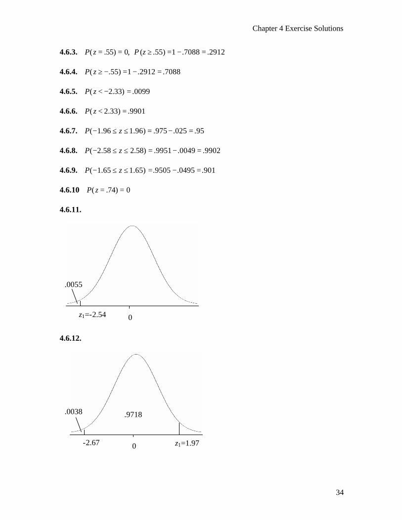
4.6.3. ( .55) 0, ( .55) 1 .7088 .2912P z P z= = ≥ = − = 4.6.4. ( .55) 1 .2912 .7088P z ≥ − = − = 4.6.5. ( 2.33) .0099P z < − = 4.6.6. ( 2.33) .9901P z < = 4.6.7. ( 1.96 1.96) .975 .025 .95P z− ≤ ≤ = − = 4.6.8. ( 2.58 2.58) .9951 .0049 .9902P z− ≤ ≤ = − = 4.6.9. ( 1.65 1.65) .9505 .0495 .901P z− ≤ ≤ = − = 4.6.10 ( .74) 0P z = = 4.6.11.
4.6.12.
0 z1=-2.54
.0055
0 -2.67
.9718
z1=1.97
.0038

Chapter 4 Exercise Solutions
35
4.6.13.
4.6.14.
4.6.15.
0
.9616
z1=1.77
.0384
1-.0384=.9616
0
.8132
-z1=-1.32
.0932
z1 =1.32
.0932
(1-.8132)/2=.0934
0
.8869
z1=1.21
.1117
P(z < 2.98) = .9986; .9986 -.1117 = .8869
2.98
Chapter 4 Exercise Solutions
36
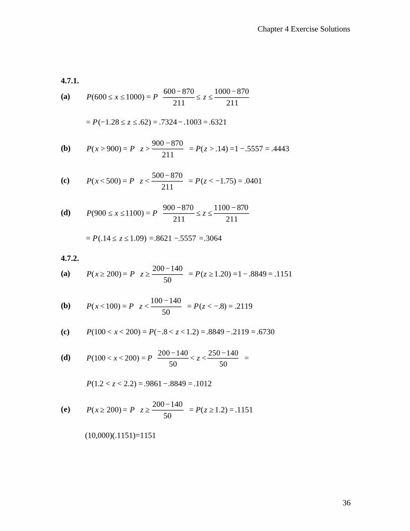
4.7.1.
(a) 600 870 1000 870
(600 1000)211 211
P x P z− − ≤ ≤ = ≤ ≤
( 1.28 .62) .7324 .1003 .6321P z= − ≤ ≤ = − =
(b) 900 870
( 900) ( .14) 1 .5557 .4443211
P x P z P z− > = > = > = − =
(c) 500 870
( 500) ( 1.75) .0401211
P x P z P z− < = < = < − =
(d) 900 870 1100 870
(900 1100)211 211
P x P z− − ≤ ≤ = ≤ ≤
(.14 1.09) .8621 .5557 .3064P z= ≤ ≤ = − =
4.7.2.
(a) 200 140
( 200) ( 1.20) 1 .8849 .115150
P x P z P z− ≥ = ≥ = ≥ = − =
(b) 100 140
( 100) ( .8) .211950
P x P z P z− < = < = < − =
(c) (100 200) ( .8 1.2) .8849 .2119 .6730P x P z< < = − < < = − =
(d) 200 140 250 140(100 200)
50 50P x P z
− − < < = < < =
(1.2 2.2) .9861 .8849 .1012P z< < = − =
(e) 200 140
( 200) ( 1.2) .115150
P x P z P z− ≥ = ≥ = ≥ =
(10,000)(.1151)=1151

Chapter 4 Exercise Solutions
37
4.7.3.
(a) 15 30.23
( 15) ( 1.10) .135713.84
P x P z P z− < = < = < − =
(b) 40 30.23
( 40) ( .71) .1 .7611 .238913.84
P x P z P z− > = > = > = − =
(c) 14 30.23 40 30.23
(14 50)13.84 13.84
P x P z− − ≤ ≤ = ≤ ≤
( 1.17 .71) .7611 .1210 .6401P z= − ≤ ≤ = − =
(d) 10 30.23
( 10) ( 1.46) .072113.84
P x P z P z− < = < = < − =
(e) 10 30.23 20 30.23
(10 20)13.84 13.84
P x P z− − ≤ ≤ = ≤ ≤
( 1.46 .74) .2296 .0721 .1575P z= − ≤ ≤ − = − =
4.7.4.
(a) 50 60
( 50) ( .67) .1 .2514 .748615
P x P z P z− > = > = > − = − =
(b) 30 60
( 30) ( 2) .022815
P x P z P z− < = < = < − =
(c) 30 60 60 60
(30 60)15 15
P x P z− − < < = < <
( 2 0) .4772P z= − < < =
(d) 90 60
( 90) ( 2) .002815
P x P z P z− > = > = > =
Chapter 4 Exercise Solutions
38
4.7.5.
(a) 180 200 200 200
(180 200) ( 1 0) .341320 20
P x P z P z− − < < = < < = − < < =
(b) 225 200
( 225) ( 1.25) 1 .9844 .105620
P x P z P z− > = > = > = − =
(c) 150 200
( 150) ( 2.5) .006220
P x P z P z− < = < = < − =
(d) 190 200 210 200
(190 210)20 20
P x P z− − < < = < < =
( .5 .5) .6915 .3085 .3830P z− < < = − =
4.7.6.
(a) 50 75 100 75
( 1 .1) .8413 .1587 .682625 25
P z P z− − ≤ ≤ = − ≤ ≤ = − =
(b) 90 75
( .6) 1 .7257 .274325
P z P z− > = > = − =
(c) 60 75
( .6) .274325
P z P z− < = < − =
(d) 85 75
( .4) 1 .6554 .344625
P z P z− ≥ = ≥ = − =
(e) 30 75 110 75
( 1.8 1.4) .9192 .0359 .883325 25
P z P z− − ≤ ≤ = − ≤ ≤ = − =
4.7.7.
(a) 155 132
( 155) ( 1.53) 1 .9370 .063015
P x P z P z− > = > = > = − =
(b) 100 132
( 100) ( 2.13) .016615
P x P z P z− ≤ = < = ≤ − =
.0166
Chapter 4 Exercise Solutions
39
(c) 105 132 145 132
(105 145)15 15
P x P z− − < < = < < =
( 1.8 .87) .8078 .0359 .7719P z− < < = − =
Chapter 4 Review Exercises 15. (a) 3 7
10 7 .65 .35 .0212C = (b) 1-.9051=.0949 (c) 10 010 0 .65 .35C = .0135
(d) .9740-.2616=.7124 16. (a) .056 - .0118 = .0442 (b) .0118 (c) .9947 – .3557 = .6390 17. (a) .077-.043=.034 (b) .467 -.000=.467 (c) 1-.077=.923 (d) .010 (e) .127-.022=.105 18. (a) .857 – .677 = .180 (b) .677 (c) .983 – .677 = .306 19. (a) 1-.5033=.4967 (b) .5033 (c) .1678 (d) 1-.9896=.0104 (e) .9896-.1678=.8218 20. (a) .273 (b) 1 – .273 =.727 (c) .989 21.
(a) 75 60
( 75) ( 1.5) 1 .9332 .066810
P x P z P z− > = > = > = − =
(b) 55 60 75 60
(55 75)10 10
P x P z− − ≤ ≤ = ≤ =
( .5 1.5) .9332 .3085 .6247P z− ≤ ≤ = − =
(c) 50 60 70 60
(50 70) ( 1 1) .8413 .1587 .682610 10
P x P z P z− − ≤ ≤ = ≤ = − ≤ ≤ = − =
Chapter 4 Exercise Solutions
40
22.
(a) 4 10
( 4) .02283
P x P z− < = < =
(b) 5 10
( 5) 1 .0475 .95253
P x P z− > = > = − =
(c) 3 10
( 3) ( 2.33) .00993
P x P z P z− ≤ = ≤ = ≤ − =
23.
(a) 200 500
( 200) ( 3) .0013100
P x P z P z− < = < = < − =
.0013
(b) 650 500
( 650) ( 1.5) 1 .9332 .0668100
P x P z P z− ≥ = ≥ = ≥ = − =
(c) 350 500 675 500
(350 675)100 100
P x P z− − ≤ ≤ = ≤ ≤
( 1.5 1.75) .9599 .0668 .8931P z= − ≤ ≤ = − =
24. 2 20,20 , 20/ ; (1 ),16 (1 ) 16 20(1 )np np n p np p p p p
pµ σ= = = = − = − ⇒ = −
20
.2, 100.2
p n⇒ = = =
25. 0 0; ( ) .0985;1 .0985 .9015x
z P z zµ
σ−
= ≥ = − =
70
( 1.29) .9015;1.29 70 12.90 57.1010
P zµ
µ µ−
≤ = = ⇒ − = ⇒ =
Chapter 4 Exercise Solutions
41
26.
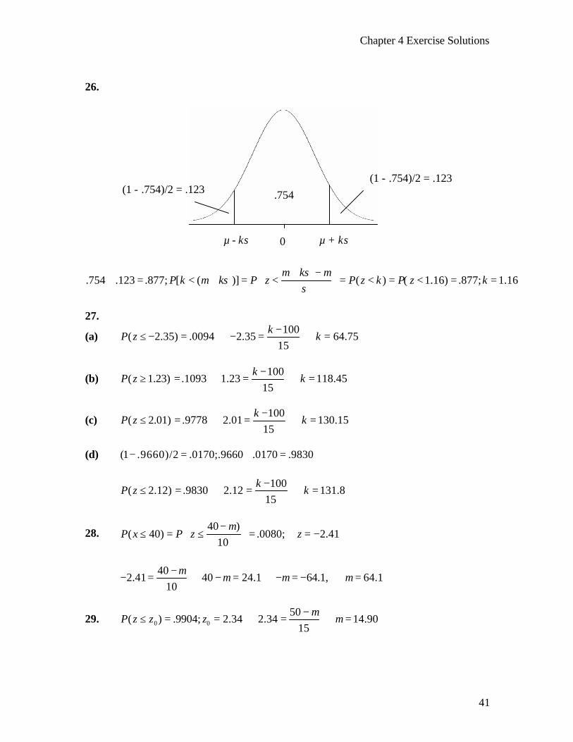
.754 .123 .877; [ ( )] ( ) ( 1.16) .877; 1.16k
P k k P z P z k P z kµ σ µ
µ σσ
+ − + = < + = < = < = < = =
27.
(a) 100
( 2.35) .0094 2.35 64.7515
kP z k
−≤ − = ⇒ − = ⇒ =
(b) 100
( 1.23) .1093 1.23 118.4515
kP z k
−≥ = ⇒ = ⇒ =
(c) 100
( 2.01) .9778 2.01 130.1515
kP z k
−≤ = ⇒ = ⇒ =
(d) (1 .9660)/2 .0170;.9660 .0170 .9830− = + =
100
( 2.12) .9830 2.12 131.815
kP z k
−≤ = ⇒ = ⇒ =
28. 40 )
( 40) .0080; 2.4110
P x P z zµ− ≤ = ≤ = = −
40
2.41 40 24.1 64.1, 64.110
µµ µ µ
−− = ⇒ − = ⇒ − = − ⇒ =
29. 0 0
50( ) .9904; 2.34 2.34 14.90
15P z z z
µµ
−≤ = = ⇒ = ⇒ =
0
.754
µ - ks
(1 - .754)/2 = .123 (1 - .754)/2 = .123
µ + ks
Chapter 4 Exercise Solutions
42
30. 25
( 25) .05265
P x P zµ− ≥ = ≥ =
z = 1.62 since ( 1.62) 1 .0526 .9474P z < = − =
25
1.62 25 8.1 16.95
µµ µ
−⇒ = ⇒ − = ⇒ =
31. 0 0
10 25( ) .0778; 1.42; 1.42 10.6P z z z σ
σ−
≤ = = − − = ⇒ =
32. 50 30
( 50) .9772; 2P x P z zσ− ≤ = ≤ = =
50 30
2 2 50 30 10σ σσ−
= ⇒ = − ⇒ =
33. (a) Could be Bernoulli if we assume each child has an equal chance of being a boy or
girl;
(b) Not a Bernoulli - More than 2 possible outcomes (c) Not a Bernoulli - Weight is a continuous variable 34. (a) Not a Bernoulli - Not a Yes/No outcome (b) Not a Bernoulli - Degrees Celsius is a continuous variable (c) Not a Bernoulli - Not a constant probability of vital signs being normal from
patient to patient
Chapter 5 Exercise Solutions
43
Chapter 5
5.3.1. Sampling distribution mean: 204, Standard Error: 44
6.222550
xn
σσ = = =
5.3.2.
(a) 1 2
170 183 195 18343/ 60 5.5513, 2.34, 2.16;
5.5513 5.5513x z zσ− −
= = = = − = =
(170 195) ( 2.34 2.16) .9846 .0096 .9747P x P z≤ ≤ = − ≤ ≤ = − =
(b) 175 183
1.44; ( 175) ( 1.44) .07495.5513
z P x P z−
= = − < = < − =
(c) 190 183
1.26; ( 190) 1 ( 1.26) 1 .8962 .10385.5513
z P x P z−
= = > = − ≤ = − =
5.3.3.
(a) 6 5.7
1/ 9 .3333, .90, ( 6) 1 ( .90) 1 .8159 .1841.3333x z P x P zσ−
= = = = > = − ≤ = − =
(b) 1 2
5 5.72.10, .90
.3333z z
−= = − =
(5 6) ( 2.10 .90) .8159 .0179 .7980P x P z≤ ≤ = − ≤ ≤ = − =
(c) 5.2 5.7
1.50, ( 5.2) ( 1.50) .0668.3333
z P x P z−
= = − < = < − =
5.3.4.
(a) 800 721
454/ 50 64.2053, 1.2364.2053x zσ
−= = = =
( 800) 1 ( 1.23) 1 .8907 .1093P x P z> = − ≤ = − =
(b) 700 721
.33, ( 700) ( .33) .370764.2053
z P x P z−
= = − < = < − =
(c) 1 2
850 721.33, 2.01
64.2053z z
−= − = =
(700 850) ( .33 2.01) .9778 .3707 .6071P x P z≤ ≤ = − ≤ ≤ = − =
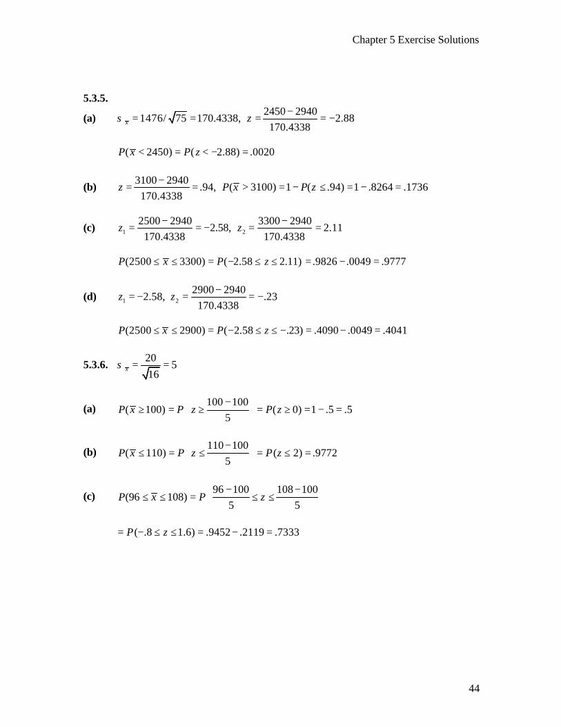
Chapter 5 Exercise Solutions
44
5.3.5.
(a) 2450 2940
1476/ 75 170.4338, 2.88170.4338x zσ
−= = = = −
( 2450) ( 2.88) .0020P x P z< = < − =
(b) 3100 2940
.94, ( 3100) 1 ( .94) 1 .8264 .1736170.4338
z P x P z−
= = > = − ≤ = − =
(c) 1 2
2500 2940 3300 29402.58, 2.11
170.4338 170.4338z z
− −= = − = =
(2500 3300) ( 2.58 2.11) .9826 .0049 .9777P x P z≤ ≤ = − ≤ ≤ = − =
(d) 1 2
2900 29402.58, .23
170.4338z z
−= − = = −
(2500 2900) ( 2.58 .23) .4090 .0049 .4041P x P z≤ ≤ = − ≤ ≤ − = − =
5.3.6. 20
516
xσ = =
(a) 100 100
( 100) ( 0) 1 .5 .55
P x P z P z− ≥ = ≥ = ≥ = − =
(b) 110 100
( 110) ( 2) .97725
P x P z P z− ≤ = ≤ = ≤ =
(c) 96 100 108 100
(96 108)5 5
P x P z− − ≤ ≤ = ≤ ≤
( .8 1.6) .9452 .2119 .7333P z= − ≤ ≤ = − =
Chapter 5 Exercise Solutions
45
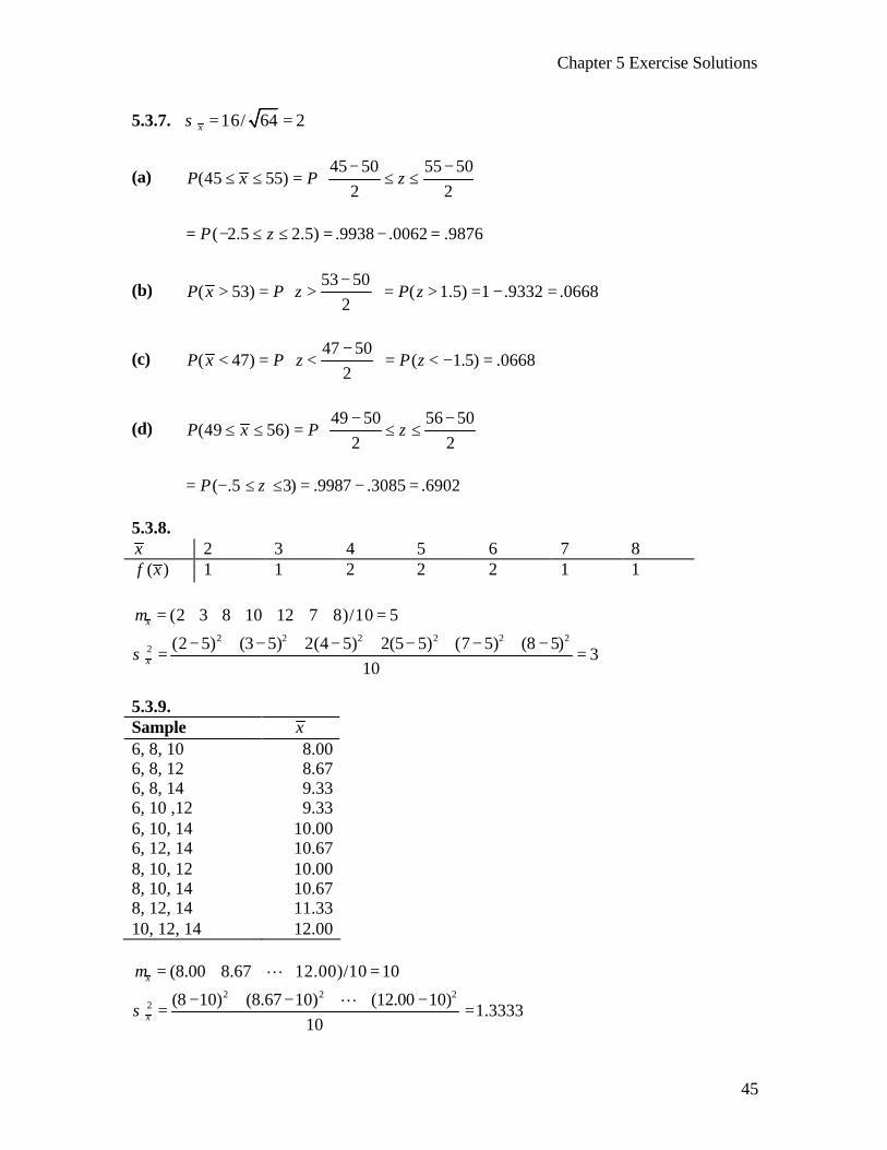
5.3.7. 16/ 64 2xσ = =
(a) 45 50 55 50
(45 55)2 2
P x P z− − ≤ ≤ = ≤ ≤
( 2.5 2.5) .9938 .0062 .9876P z= − ≤ ≤ = − =
(b) 53 50
( 53) ( 1.5) 1 .9332 .06682
P x P z P z− > = > = > = − =
(c) 47 50
( 47) ( 1.5) .06682
P x P z P z− < = < = < − =
(d) 49 50 56 50
(49 56)2 2
P x P z− − ≤ ≤ = ≤ ≤
( .5 3) .9987 .3085 .6902P z= − ≤ ≤ = − =
5.3.8. x 2 3 4 5 6 7 8
( )f x 1 1 2 2 2 1 1
(2 3 8 10 12 7 8)/10 5xµ = + + + + + + = 2 2 2 2 2 2
2 (2 5) (3 5) 2(4 5) 2(5 5) (7 5) (8 5)3
10xσ− + − + − + − + − + −
= =
5.3.9. Sample x 6, 8, 10 8.00 6, 8, 12 8.67 6, 8, 14 9.33 6, 10 ,12 9.33 6, 10, 14 10.00 6, 12, 14 10.67 8, 10, 12 10.00 8, 10, 14 10.67 8, 12, 14 11.33 10, 12, 14 12.00
(8.00 8.67 12.00)/10 10xµ = + + + =L 2 2 2
2 (8 10) (8.67 10) (12.00 10)1.3333
10xσ− + − + + −
= =L
Chapter 5 Exercise Solutions
46
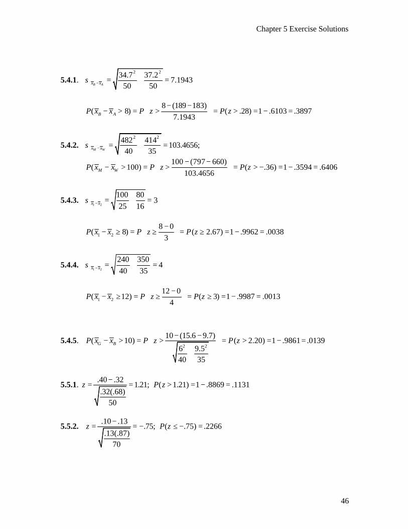
5.4.1. 2 234.7 37.2
7.194350 50B Ax xσ − = + =
8 (189 183)
( 8) ( .28) 1 .6103 .38977.1943B AP x x P z P z
− − − > = > = > = − =
5.4.2. 2 2482 414
103.4656;40 35M Wx xσ − = + =
100 (797 660)( 100) ( .36) 1 .3594 .6406
103.4656M WP x x P z P z− − − > = > = > − = − =
5.4.3. 1 2
100 803
25 16x xσ − = + =
1 2
8 0( 8) ( 2.67) 1 .9962 .0038
3P x x P z P z
− − ≥ = ≥ = ≥ = − =
5.4.4. 1 2
240 3504
40 35x xσ − = + =
1 2
12 0( 12) ( 3) 1 .9987 .0013
4P x x P z P z
− − ≥ = ≥ = ≥ = − =
5.4.5. 2 2
10 (15.6 9.7)( 10) ( 2.20) 1 .9861 .0139
6 9.540 35
G BP x x P z P z
− − − > = > = > = − =
+
5.5.1. .40 .32
1.21; ( 1.21) 1 .8869 .1131.32(.68)
50
z P z−
= = > = − =
5.5.2. .10 .13
.75; ( .75) .2266.13(.87)
70
z P z−
= = − ≤ − =
Chapter 5 Exercise Solutions
47
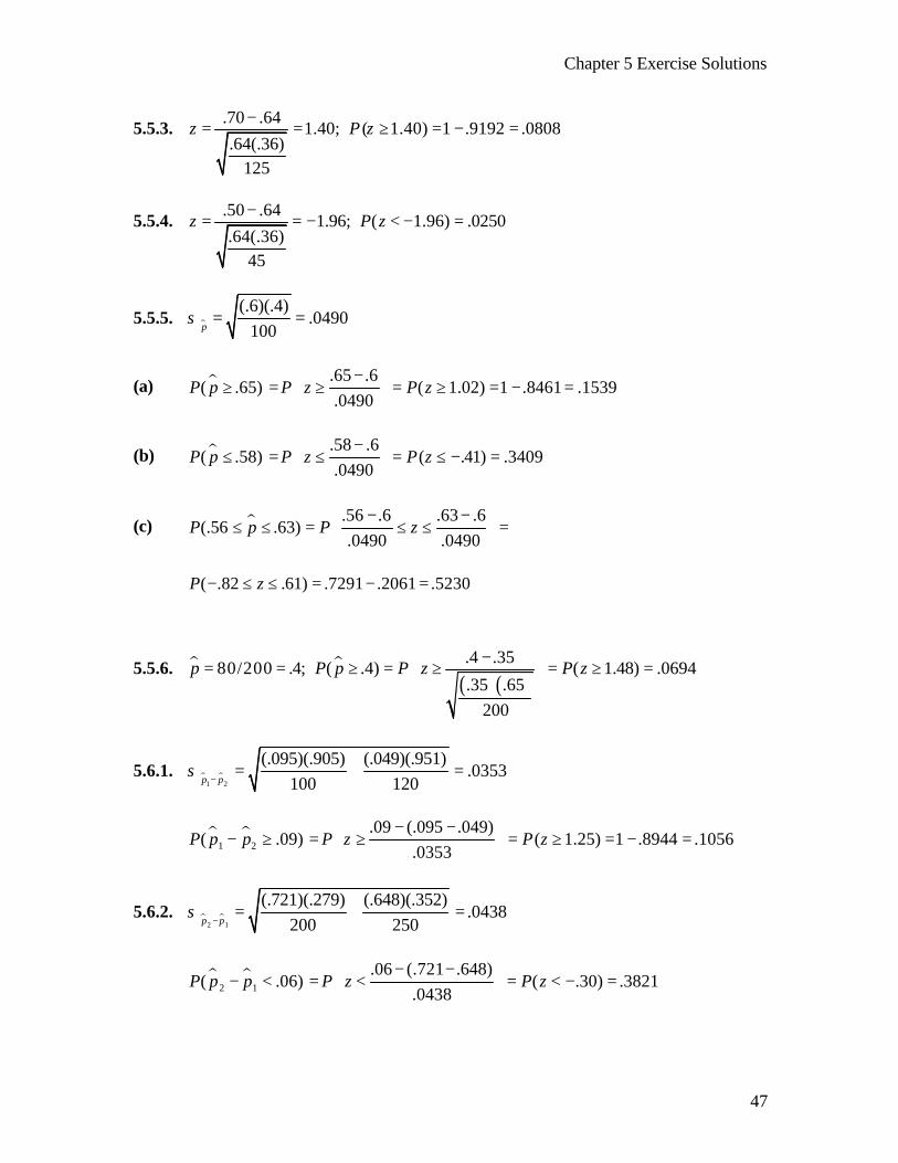
5.5.3. .70 .64
1.40; ( 1.40) 1 .9192 .0808.64(.36)
125
z P z−
= = ≥ = − =
5.5.4. .50 .64
1.96; ( 1.96) .0250.64(.36)
45
z P z−
= = − < − =
5.5.5. µ(.6)(.4)
.0490100p
σ = =
(a) µ .65 .6( .65) ( 1.02) 1 .8461 .1539
.0490P p P z P z
− ≥ = ≥ = ≥ = − =
(b) µ .58 .6( .58) ( .41) .3409
.0490P p P z P z
− ≤ = ≤ = ≤ − =
(c) µ .56 .6 .63 .6(.56 .63)
.0490 .0490P p P z
− − ≤ ≤ = ≤ ≤ =
( .82 .61) .7291 .2061 .5230P z− ≤ ≤ = − =
5.5.6. µ µ( )( ).4 .35
80/200 .4; ( .4) ( 1.48) .0694.35 .65
200
p P p P z P z
− = = ≥ = ≥ = ≥ =
5.6.1. µ µ1 2
(.095)(.905) (.049)(.951).0353
100 120p pσ
−= + =
µ µ1 2
.09 (.095 .049)( .09) ( 1.25) 1 .8944 .1056
.0353P p p P z P z
− − − ≥ = ≥ = ≥ = − =
5.6.2. µ µ2 1
(.721)(.279) (.648)(.352).0438
200 250p pσ
−= + =
µ µ2 1
.06 (.721 .648)( .06) ( .30) .3821
.0438P p p P z P z
− − − < = < = < − =
Chapter 5 Exercise Solutions
48
5.6.3. µ µ1 2
(.21)(.79) (.13)(.87).0475
120 130p pσ
−= + =
µ µ1 2
.04 .08 .20 .08(.04 .20) ( .84 2.53) .9943 .2005 .7938
.0475 .0475P p p P z P z
− − < − < = < < = − < < = − =
Chapter 5 Review Exercises
10. 12 15
( 12) ( 3) 1 .0013 .99874 / 4
P x P z P z− ≥ = ≥ = ≥ − = − =
11. 25 23.1
( 25) ( 3.44) 1 .9997 .00033.7/ 45
P x P z P z−
> = > = > = − =
12. 24 24.7
( 24) ( 1.50) .06683.3/ 50
P x P z P z−
< = < = < − =
13. 2 23.3 3.7
.722550 45M Wx xσ − = + =
3 (24.7 23.1)
( 3) ( 1.94) 1 .9738 .0262.7225M WP x x p z P z
− − − > = > = > = − =
14. 12 13.7
( 12) ( 1.91) .02818.9/ 100
P x P z P z−
< = < = < − =
15. 19 17.9
( 19) ( 1.11) 1 .8665 .133510.9/ 120
P x P z P z−
> = > = > = − =
16. 2 210.9 8.9
1.3350120 100M Wx xσ − = + =
5 (17.9 13.7)
( 5) ( .60) 1 .7257 .27431.3350M WP x x p z P z
− − − > = > = > = − =
Chapter 5 Exercise Solutions
49
17. µ .25 .19( .25) ( 1.23) 1 .8907 .1093
(.19)(.81)65
P p P z P z
− > = > = > = − =
18. µ .20 .17( .20) ( 1.18) 1 .8810 .1190
(.17)(.83)220
P p P z P z
− > = > = > = − =
19. µ .20 .23( .20) ( 1.13) .1292
(.23)(.77)250
P p P z P z
− < = < = < − =
20. µ µ(.23)(.77) (.17)(.83)
.0367250 220M Wp p
σ−
= + =
µ µ .05 (.23 .17)( .05) ( .27) .3936
.0367M WP p p P z P z− − − < = < = < − =
21. 10 5
10!252
5!5!C = =
22. Normally distributed 23. µ µ.53, (.53)(.47)/110 .0476
p pµ σ= = =
24. µ .50 .53( .50) ( .63) .2643
.0476P p P z P z
− < = < = < − =
25. At least approximately normally distributed 26. 25, 7 / 35 1.18x xµ σ= = =
27. 22 25 29 25
(22 29)1.18 1.18
P x P z− − ≤ ≤ = ≤ ≤
( 2.54 3.39) .9997 .0055 .9942P z= − ≤ ≤ = − =
Chapter 5 Exercise Solutions
50
28. (a) n = 10 – Normal n = 50 – Normal n = 200 – Normal (b) n = 10 – Normal n = 50 – Normal n = 200 – Normal (c) n = 10 – Not normal n = 50 – Approx. normal n = 200 – Approx. normal 29. (a) No, since 8(.5) = 4 and 4<5. (b) Yes, since 30(.4) = 12 and 30(.6) = 18 are both >5. (c) No, since 30(.1) = 3 is less than 5. (d) Yes, since 1000(.01) = 10 and 1000(.99)=990 are both greater than 5. (e) Yes, since 100(.9)=90 and 100(.1) = 10 are both greater than 5. (f) Yes, since 150(.05)=7.5 and 150(.95) = 142.5 are both greater than 5.
Chapter 6 Exercise Solutions
51
Chapter 6 6.2.1. 10/ 49 1.43xσ = = (a) 90 1.645(1.43) (88,92)± = (b) 90 1.96(1.43) (87,93)± = (c) 90 2.58(1.43) (86,94)± = 6.2.2. 3.5/ 16 .875xσ = = (a) 5.98 1.645(.875) (4.54,7.42)± = (b) 5.98 1.96(.875) (4.26,7.70)± = (c) 5.98 2.58(.875) (3.72,8.24)± = 6.2.3. 3 / 64 .375xσ = = (a) 8.25 1.645(.375) (7.63,8.87)± = (b) 8.25 1.96(.375) (7.51,8.99)± = (c) 8.25 2.58(.375) (7.28,9.22)± = 6.2.4. 15/ 100 1.5xσ = = (a) 125 1.645(1.5) (123.53,127.47)± = (b) 125 1.96(1.5) (122.06,127.94)± = (c) 125 2.58(1.5) (121.13,128.87)± = 6.2.5. 1747.625, 350/ 16 87.5xx σ= = = (a) 1747.625 1.645(87.5) (1603.688,1891.563)± = (b) 1747.625 1.96(87.5) (1576.125,1919.125)± = (c) 1747.625 2.58(87.5) (1521.875,1973.375)± = 6.3.1. (a) 2.1448 (b) 2.8073 (c) 1.8946 (d) 2.0452
Chapter 6 Exercise Solutions
52
6.3.2. (a) (11 10 6 3 11 10 9 11)/8 8.875x = + + + + + + + =
(b) 2( 8.875)
2.9007
ixs
−= =∑
(c) 2.900/ 8 1.0253= (d) 8.875 2.3646(1.0253) (6.4506,11.2994)± = (e) 2.3646(1.0253) 2.4244= (f) Approximately 95% of all intervals constructed in a similar manner with sample
of 8 drawn from the population will contain the sample mean. (g) We are 95% confident the population mean is between 6.4506 and 11.2994. 6.3.3. (a) ( ) ( ) ( ) ( ).4 15 1.549; .1 15 .387= =
(b) 3.5 2.1448(.4) (2.64,4.36); .7 2.1448(.1) (.49,.91)± = ± = (c) Nitric oxide diffusion rates are normally distributed in the population from which the
sample was drawn. (d) Practical: We are 95% confident the mean maximal nitric oxide diffusion rate for
asthmatic schoolchildren is between 2.64 and 4.36 while for control subjects it is between .49 and .91. Probabilistic: approximately 95% of intervals constructed ina similar manner with samples of size 15 drawn from the populations of asthmatic and control schoolchildren will contain the respective population means.
(e) The practical. (f) Narrower because the t coefficient from which the interval is constructed is smaller. (g) Wider because the t coefficient from which the interval is constructed is larger.
Chapter 6 Exercise Solutions
53
6.3.4. (a) 4.3/ 9 1.4333xs = = (b) 17.4 3.3554(1.433) (12.59,22.21)± = (c) 13.3554(1.433) 19.14= (d) That the distribution for the population of subjects with ACL-deficient knees is normally
distributed. 6.3.5. 12/ 16 3xs = = 90 % CI: 71.5 1.7530(3) (66.2,76.8)± = 95 % CI: 71.5 2.1315(3) (65.1,77.9)± = 99 % CI: 71.5 2.9467(3) (62.7,80.3)± = 6.3.6. 25.9, 9.4687, 9.4687/ 10 2.9943xx s s= = = = 25.9 2.2622(2.9943) (19.13,32.67)± = 6.4.1. The samples constitute independent simple random samples from the two populations.
The two populations of free fatty acid concentrations are normally distributed, and the two population variances are equal.
1 230 18 127.2792, 62 11 205.6307s s= = = = 2 2
2 17(127.2792 ) 10(205.6307 )25860.7318, 25860.7318 160.8127
18 11 2p ps s+
= = = =+ −
90% CI: 25860.7318 25860.7318
(299 744) 1.7033 ( 549.8, 340.2)18 11
− ± + = − −
95% CI: 25860.7318 25860.7318
(299 744) 2.0518 ( 571.3, 318.7)18 11
− ± + = − −
99% CI: 25860.7318 25860.7318
(299 744) 2.7707 ( 615.5, 274.5)18 11
− ± + = − −
Chapter 6 Exercise Solutions
54
6.4.2. The samples constitute independent simple random samples from the two populations. The two populations of prostate cancer screening knowledge scores are normally distributed, and the two population variances are equal.
1 2
2 25.8 5.8.7570
185 86x xσ − = + =
90 %CI: (20.6 17.4) 1.645(.7570) (1.95,4.45)− ± = 95 % CI: (20.6 17.4) 1.96(.7570) (1.72,4.68)− ± = 99 %CI (20.6 17.4) 2.58(.7570) (1.25,5.15)− ± = 6.4.3. The samples constitute independent simple random samples from the two populations.
The two populations of pain scores are normally distributed, and the two population variances are equal.
1 25.5 40 34.7851 4.6 57 34.7292s s= = = =
1 2
2 234.7851 34.72927.1701
40 57x xσ − = + =
90 % CI: (36.4 30.5) 1.645(7.1701) ( 5.89,17.69)− ± = − 95 % CI: (36.4 30.5) 1.96(7.1701) ( 8.15,19.95)− ± = − 99 % CI: (36.4 30.5) 2.58(7.1701) ( 12.60,24.40)− ± = −

Chapter 6 Exercise Solutions
55
6.4.4. The samples constitute independent simple random samples from the two populations.
The two populations of pain scores are normally distributed, and the two population variances are equal.
18.83, 4.36, 22.21, 3.36F F M Mx s x s= = = =
2 2
2 5(4.36) 13(3.36)13.4340, 13.4340 3.6652
6 14 2p ps s+
= = = =+ −
90 % CI: 2 23.6652 3.6652
(18.83 22.21) 1.7341 ( 6.48, .28)6 14
− ± + = − −
95 % CI: 2 23.6652 3.6652
(18.83 22.21) 2.1009 ( 7.14,.38)6 14
− ± + = −
90 % CI: 2 23.6652 3.6652
(18.83 22.21) 2.8784 ( 8.53,1.77)6 14
− ± + = −
6.4.5. The samples constitute independent simple random samples from the two populations.
The two populations of doses of methadone are normally distributed, and the two population variances are equal.
2 2
2 8(156) 7(316)59578.6667, 59578.6667 244.0874
9 8 2p ps s+
= = = =+ −
90 % CI: 2 2244.0874 244.0874
(541 269) 1.7530 (64.1,479.9)9 8
− ± + =
95 % CI: 2 2244.0874 244.0874
(541 269) 2.1314 (19.2,524.8)9 8
− ± + =
99 % CI: 2 2244.0874 244.0874
(541 269) 2.9467 ( 77.5,621.5)9 8
− ± + = −
Chapter 6 Exercise Solutions
56
6.4.6. 2 2
2 11(1.05) 8(1.01)1.0678
11 8ps+
= =+
1.0678 1.0678
.455712 9M Fx xs − = + =
90 % CI: (13.21 11.00) 1.7291(.4557) (1.42,3.00)− ± = 95 % CI: (13.21 11.00) 2.0930(.4557) (1.26,3.16)− ± = 99 % CI: (13.21 11.00) 2.8609(.4557) (.91,3.51)− ± =
6.4.7. 2 2
2 11(1.5) 11(2.0)3.125
11 11ps+
= =+
1 2
3.125 3.125.7217
12 12x xs − = + =
90 % CI: (11.1 7.8) 1.7171(.7217) (2.1,4.5)− ± = 95 % CI: (11.1 7.8) 2.0739(.7217) (1.8,4.8)− ± = 99 % CI: (11.1 7.8) 2.8188(.7217) (1.3,5.3)− ± =
6.4.8. 2 2
2 10(5) 13(6)31.2174
10 13ps+
= =+
1 2
31.2174 31.21742.2512
11 14x xs − = + =
90% CI: (26 21) 1.7139(2.2512) (1.1,8.9)− ± = 95% CI: (26 21) 2.0687(2.2512) (.3,9.7)− ± = 99% CI: (26 21) 2.8073(2.2512) ( 1.3,11.3)− ± = −
Chapter 6 Exercise Solutions
57
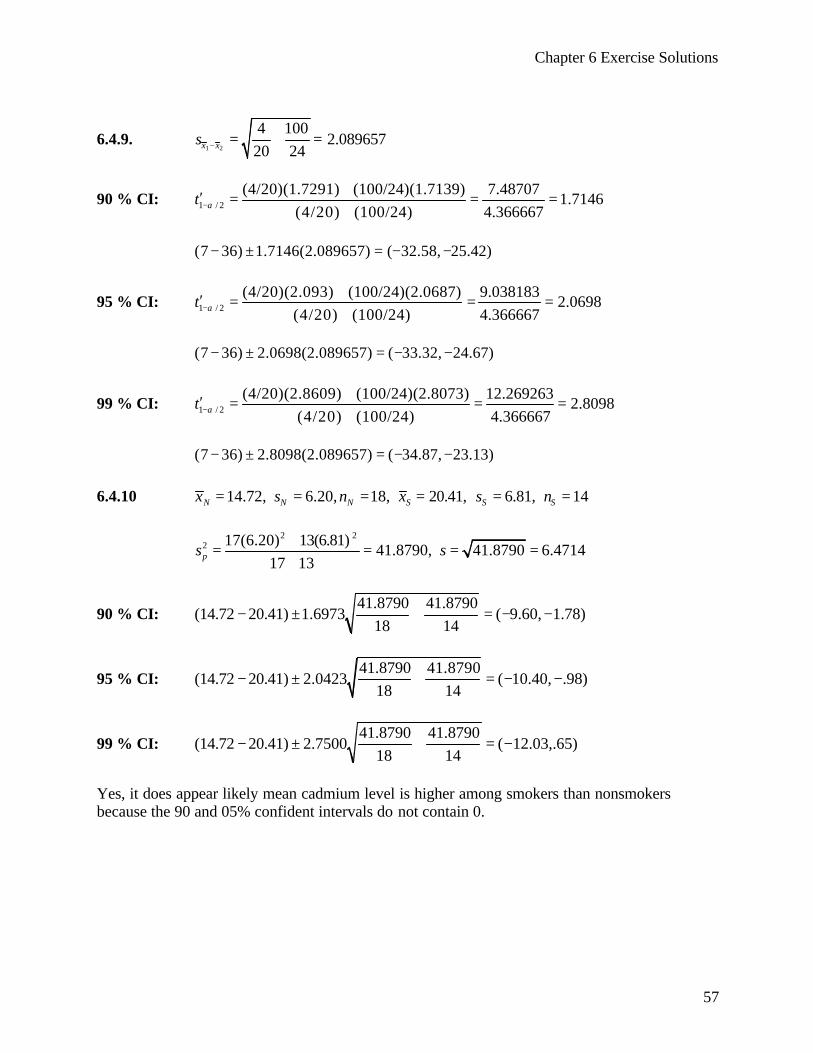
6.4.9. 1 2
4 1002.089657
20 24x xs − = + =
90 % CI: 1 / 2(4/20)(1.7291) (100/24)(1.7139) 7.48707
1.7146(4/20) (100/24) 4.366667
t α−+′ = = =+
(7 36) 1.7146(2.089657) ( 32.58, 25.42)− ± = − −
95 % CI: 1 / 2(4/20)(2.093) (100/24)(2.0687) 9.038183
2.0698(4/20) (100/24) 4.366667
t α−+′ = = =+
(7 36) 2.0698(2.089657) ( 33.32, 24.67)− ± = − −
99 % CI: 1 / 2(4/20)(2.8609) (100/24)(2.8073) 12.269263
2.8098(4/20) (100/24) 4.366667
t α−+′ = = =+
(7 36) 2.8098(2.089657) ( 34.87, 23.13)− ± = − − 6.4.10 14.72, 6.20, 18, 20.41, 6.81, 14N N N S S Sx s n x s n= = = = = =
2 2
2 17(6.20) 13(6.81)41.8790, 41.8790 6.4714
17 13ps s+
= = = =+
90 % CI: 41.8790 41.8790
(14.72 20.41) 1.6973 ( 9.60, 1.78)18 14
− ± + = − −
95 % CI: 41.8790 41.8790
(14.72 20.41) 2.0423 ( 10.40, .98)18 14
− ± + = − −
99 % CI: 41.8790 41.8790
(14.72 20.41) 2.7500 ( 12.03,.65)18 14
− ± + = −
Yes, it does appear likely mean cadmium level is higher among smokers than nonsmokers because the 90 and 05% confident intervals do not contain 0.
Chapter 6 Exercise Solutions
58
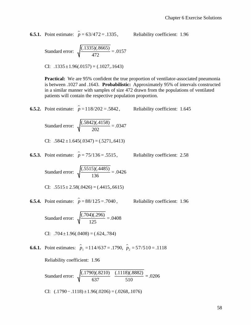
6.5.1. Point estimate: µ 63/472 .1335p = = , Reliability coefficient: 1.96
Standard error: (.1335)(.8665)
.0157472
=
CI: .1335 1.96(.0157) (.1027,.1643)± =
Practical: We are 95% confident the true proportion of ventilator-associated pneumonia is between .1027 and .1643. Probabilistic: Approximately 95% of intervals constructed in a similar manner with samples of size 472 drawn from the populations of ventilated patients will contain the respective population proportion.
6.5.2. Point estimate: µ 118/202 .5842p = = , Reliability coefficient: 1.645
Standard error: (.5842)(.4158)
.0347202
=
CI: .5842 1.645(.0347) (.5271,.6413)± =
6.5.3. Point estimate: µ 75/136 .5515p = = , Reliability coefficient: 2.58
Standard error: (.5515)(.4485)
.0426136
=
CI: .5515 2.58(.0426) (.4415,.6615)± =
6.5.4. Point estimate: µ 88/125 .7040p = = , Reliability coefficient: 1.96
Standard error: (.704)(.296)
.0408125
=
CI: .704 1.96(.0408) (.624,.784)± =
6.6.1. Point estimates: µ µ1 2114/637 .1790, 57/510 .1118p p= = = =
Reliability coefficient: 1.96
Standard error: (.1790)(.8210) (.1118)(.8882)
.0206637 510
+ =
CI: (.1790 .1118) 1.96(.0206) (.0268,.1076)− ± =

Chapter 6 Exercise Solutions
59
Practical: We are 95% confident the true difference in proportions between the abused or neglected group and the control group is between .0268 and .1076. Probabilistic: Approximately 95% of intervals constructed in a similar manner with samples of size 637 and 510 drawn from the two populations will contain the difference in the respective population proportions.
6.6.2. Point estimates: µ µ
1 2109/138 .7899, 120/136 .8824p p= = = = Reliability coefficient: 1.96
Standard error: (.7899)(.2101) (.8824)(.1176)
.0443138 136
+ =
CI: (.7899 .8824) 1.96(.0443) ( .1793, .0057)− ± = − −
6.6.3. Point estimates: µ µ
1 216/49 .3265, 12/51 .2353p p= = = = Reliability coefficient: 1.96
Standard error: (.3265)(.6735) (.2353)(.7647)
.089549 51
+ =
CI: (.3265 .2353) 1.96(.0895) ( .0842,.2666)− ± = −
6.6.4. Point estimates: µ µ1 224/50 .48, 50/75 .6667p p= = = =
Reliability coefficient: 1.645
Standard error: (.48)(.52) (.6667)(.3333)
.089250 75
+ =
CI: (.4800 .6667) 1.645(.0892) ( .3334, .0400)− ± = − −
6.7.1. 2 2
2
(2.58) (1)26.6256 27
.5n = = ≈
2 2
2
(1.96) (1)15.3664 16
.5n = = ≈
Chapter 6 Exercise Solutions
60
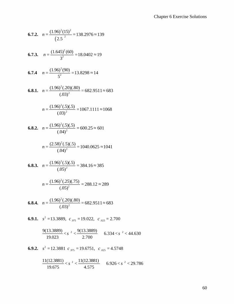
6.7.2. ( )
2 2
2
(1.96) (15)138.2976 139
2.5n = = ≈
6.7.3. 2
2
(1.645) (60)18.0402 19
3n = = ≈
6.7.4 2
2
(1.96) (90)13.8298 14
5n = = ≈
6.8.1. 2
2
(1.96) (.20)(.80)682.9511 683
(.03)n = = ≈
2
2
(1.96) (.5)(.5)1067.1111 1068
(.03)n = = ≈
6.8.2. 2
2
(1.96) (.5)(.5)600.25 601
(.04)n = = ≈
2
2
(2.58) (.5)(.5)1040.0625 1041
(.04)n = = ≈
6.8.3. 2
2
(1.96) (.5)(.5)384.16 385
(.05)n = = ≈
2
2
(1.96) (.25)(.75)288.12 289
(.05)n = = ≈
6.8.4. 2
2
(1.96) (.20)(.80)682.9511 683
(.03)n = = ≈
6.9.1. 2
.975 .02513.3889, 19.022, 2.700s χ χ= = =
2 29(13.3889) 9(13.3889)6.334 44.630
19.023 2.700σ σ< < ⇒ < <
6.9.2. 2
.975 .02512.3881 19.6751, 4.5748s χ χ= = =
2 211(12.3881) 11(12.3881)6.926 29.786
19.675 4.575σ σ< < ⇒ < <
Chapter 6 Exercise Solutions
61
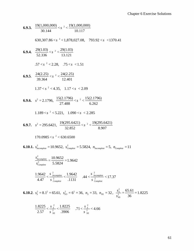
6.9.3. 219(1,000,000) 19(1,000,000)30.144 10.117
σ< <
2630,307.86 1,878,027.08, 793.92 1370.41σ σ< < < <
6.9.4. 229(1.03) 29(1.03)52.336 13.121
σ< <
2.57 2.28, .75 1.51σ σ< < < <
6.9.5. 224(2.25) 24(2.25)39.364 12.401
σ< <
21.37 4.35, 1.17 2.09σ σ< < < <
6.9.6. 2 215(2.1796) 15(2.1796)2.1796,
27.488 6.262s σ= < <
21.189 5.221, 1.090 2.285σ σ< < < <
6.9.7. 2 219(295.6421) 19(295.6421)295.6421,
32.852 8.907s σ= < <
2170.0985 630.6500σ< < 6.10.1. 2 210.9652, 5.5824, 5, 11Incomplete Complete Incomplete Completes s n n= = = =
2
2
10.96521.9642
5.5824Incomplete
Complete
s
s= =
2 2
2 2
1.9642 1.9642.44 17.37
4.47 .1131Incomplete Incomplete
Complete Complete
σ σ
σ σ< < ⇒ < <
6.10.2. 2 2 2 28.1 65.61, 6 36, 33, 32S NS S NSs s n n= = = = = = , 2
2
65.611.8225
36S
NS
ss
= =
2 2
2 2
1.8225 1.8225.71 4.66
2.57 .3906S S
NS NS
σ σσ σ
< < ⇒ < <
Chapter 6 Exercise Solutions
62
6.10.3. 2 21 12 22 2
12/10 12/10.49 2.95
2.46 1/2.46σ σσ σ
< < ⇒ < <
6.10.4. 2 21 12 22 2
15/8 15/8.78 4.5
2.40 1/2.40σ σσ σ
< < ⇒ < <
6.10.5. 2 21 12 22 2
35,000/20,000 35,000/20,000.90 3.52
1.94 1/2.01σ σσ σ
< < ⇒ < <
6.10.6. 2 21 12 22 2
148/105 148/105.39 4.75
3.62 1/3.37σ σσ σ
< < ⇒ < <
6.10.7. 2
2 22
65.0423334.066625, 65.042333, 15.99418
4.066625U
N UN
ss s
s= = = =
2 21 12 22 2
15.99418 15.994185.13 60.30
3.12 1/3.77σ σσ σ
< < ⇒ < <
Chapter 6 Review Exercises 13. x =79.87, s2 = 28.1238, s = 5.3; ( )79.87 2.1448 5.30/ 15 (76.93,82.81)± =
14. µ ( ).35, 140, .35 1.96 (.35)(.65)/140 (.27,.43)p n= = ± =
15. µ 21/70 .30, .30 1.96 (.3)(.7)/70 (.19,.41)p = = ± =
16 (a) 2
2
(1.96) (.3)(.7)322.6944 323
(.05)n = = ≈
(b) 2
2 2
1500(1.96) (.3)(.7)265.7096 266
(.05) (1499) (1.96) (.3)(.7)n = = ≈
+
17. µ µ1 244/220 .20, 150/280 .54p p= = = =
(.54)(.46) (.20)(.80)
(.54 .20) 1.96 (.26,.42)280 220
− ± + =

Chapter 6 Exercise Solutions
63
18. 2 2
2 (20)(1.95) (15)(1.70)3.41
35ps+
= =
3.41 3.41
(3.85 2.80) 2.0301 ( .19,2.29)20 15
− ± + = −
19. µ (.9)(.1)180/200 .90, .90 1.645 (.87,.93)
200p = = ± =
20. 2 225 30
(125 95) 1.96 (17.06,42.94)35 35
− ± + =
21. x = 19.23, s2 = 20.2268; 19.23 2.2622 20.2268)/10 (16.01,22.45)± = 22. 2 27.5193, .089307, 7.2717, .040452A A B Bx s x s= = = =
2 14(.089307) 11(.040452).067811
25ps+
= =
.067811 .067811
(7.5193 7.2717) 1.7081 (.0753,.4199)15 12
− ± + =
23. 2 26.125, 15.8420, 5.806, 5.9980A A B Bx s x s= = = =
2 11(15.8420) 15(5.9980)10.1628
11 15ps+
= =+
10.1628 10.1628
(6.125 5.8420) 2.0555 ( 2.18,2.82)12 16
− ± + = −
24. 2 2308 144
(358 483) 2.58 ( 246.4, 3.6)52 53
− ± + = − −
25. 215
435 1.96 (362.73,507.27)34
± =
26. (.293)(.707) (.173)(.827)
(.293 .173) 1.96 (.026,.214)220 106
− ± + =

Chapter 6 Exercise Solutions
64
27. µ (.5897)(.4103)23/39 .5897, .5897 1.96 (.4353,.7441)
39p = = ± =
28. 2 212.63167, 20.16525, 21.236, 78.15337M M H Hx s x s= = = =
20.16525 78.15337
(21.235 12.63167) 1.96 (5.903,11.305)60 50
− ± + =
29. (.0582) 10 .1840, (.1641) 10 .5189CP Cs s= = = =
Assume equal variances for the two groups, 2 2
2 9(.1840) 9(.5189).1516
18ps+
= =
.1516 .1516
(.220 .334) 1.7341 ( .416,.188)10 10
− ± + = −
30. Assume unequal variances for the two groups
2 21 2 1 28.2 /19 3.5389, 23 /17 31.1176, 2.8784, 2.9208t tω ω= = = = = =
.995
3.5389(2.8784) 31.1176(2.9208)2.9165
3.5389 31.1176t
+′ = =+
2 28.2 23
(16.4 39.8) 2.9165 ( 40.57, 6.23)19 17
− ± + = − −
31. Level of confidence decreases. The interval would have no width. The level of
confidence would be zero. 32. The interval would have to cover the entire spectrum of possible answers. The interval would be too large to be useful in any way. 33. Since the sample size is 32, the reliability coefficient should be z.
The precision of the estimate equals the margin of error, which is 8.1
34. The target population are people staying in hospitals with and without delirium. The sampled population was the 204 subjects with delirium and the 118 without delirium in the study. 35. All drivers aged 55 and older. Drivers 55 and older participating in the vision
study.
Chapter 6 Exercise Solutions
65
36. The target population is babies born of HIV-1 infected mothers. The sampled population is the babies in the sample from Cameroon. 37. .3197, .2486, 216x s n= = =
.2486
.3197 1.96 (.2865,.3529)216
± =
We use z since n >30.
38. 1.7518, .0760, 109x s n= = =
.0760
1.7518 1.645 (1.7398,1.7638)109
± =
Chapter 7 Exercise Solutions
66
Chapter 7
7.2.1. ( )0
70.7 75: 75, : 75, 2.57
14.6/ 76AH H zµ µ
−≥ < = = −
Reject H0 since -2.57 < -2.33, p = .0051 < .01
7.2.2. ( )0
54.94 60: 60, : 60, 54.94, 8.8729, 2.28
8.8729/ 16AH H x s tµ µ
−≥ < = = = = −
Reject H0 since -2.28 < -1.7530, .01 < p < .025
7.2.3. ( )0
10.3 9: 9, : 9, .76
7.3/ 18AH H tµ µ
−≤ > = =
Fail to reject H0 since .76 < 1.333, p > .10
7.2.4. ( )0
4.8 4: 4, : 4, 2.00
2 / 25AH H tµ µ
−≤ > = =
Reject H0 since 2.00 > 1.7109, .025 < p < .05 We assume the data comes from a normally distributed population.
7.2.5. ( )0
21 30: 30, : 30, 5.73
11/ 49AH H zµ µ
−≥ < = = −
Yes, Reject H0 since z = - 5.73 < - 1.645, p < .0001
7.2.6. ( )0
6.5 6: 6, : 6, 2.50
.6/ 9AH H tµ µ
−≤ > = =
Reject H0 since 2.50 > 1.8595, .01 < p < .025
7.2.7. ( )0
77 80: 80, : 80, 1.50
10/ 25AH H tµ µ
−≥ < = = −
Fail to reject H0 since t = - 1.50 > - 1.7109, .05 < p < .10
Chapter 7 Exercise Solutions
67
7.2.8. ( )0
1985 2000: 2000, : 2000, 1.60
210/ 500AH H zµ µ
−≥ < = = −
Fail to reject H0 since z = - 1.60 > - 1.645, p = .0548
7.2.9. ( )0
27 25: 25; : 25; 3.08
6.5/ 100AH H zµ µ
−≤ > = =
Reject H0 since z = 3.08 > 1.645, p = .0010
7.2.10. ( )0
74 70: 70, : 70, 1.333
12/ 16AH H tµ µ
−≤ > = =
Fail to reject H0 since t = 1.33 < 1.7530, p > .10
7.2.11. ( )0
13 10: 10, : 10, 4.0
3 / 16AH H zµ µ
−≤ > = =
Reject H0 since z = 4.0 >1.645, p < .0001
7.2.12. ( )0
13.427 12: 12, : 12, 4.311
1.282/ 15AH H tµ µ
−= ≠ = =
Reject H0 since t = 4.311 > 2.1448, p < .005(2) = .010
7.2.13. ( )0
111.60 110: 110, : 110, .1271
56.303/ 20AH H tµ µ
−= ≠ = =
Fail to Reject H0 since t = .1271 < 2.8609, p > .1(2) = .2
7.2.14. ( )0
157.5833 165: 165, : 165, 1.0530
24.3999/ 12AH H tµ µ
−≥ < = = −
Fail to Reject H0 since t = -1.0530 > 1.7959, p > .1
7.2.15. 019.46 30
: 30, : 30, 4.1817.8171/ 50
AH H zµ µ−
≥ < = = −
Reject H0 since z = -4.18 > 1.645, p < .0001

Chapter 7 Exercise Solutions
68
7.2.16. 015.6238 14
: 14, : 14, 2.19963.3829/ 21
AH H tµ µ−
≤ > = =
Reject H0 since t = 2.1996 > 1.7247, .01 < p < .025
7.2.17. 0105 100
: 100, : 100, 1.6715/ 25
AH H zµ µ−
= ≠ = =
Fail to reject H0 since z = 1.67 < 1.96, p = 2(.0475) = .095
7.2.18. 0133 130
: 130, : 130, 1.5016/ 64
AH H zµ µ−
≤ > = =
Fail to reject H0 since. z = 1.50 < 1.645, p = .0668
7.2.19. 063 70
: 70, : 70, 4.007 / 16
AH H zµ µ−
≤ > = = −
Reject H0 since z = -4.00 < -2.33, p < .0001
7.3.1. 2 2
20
39(1.27 ) 23(2.64): , : , 3.6001
62MS R A MS R pH H sµ µ µ µ+
≥ < = =
(22.41 27.75)
10.90013.6001 3.6001
40 24
t−
= = −+
Reject H0 since -10.9001 < -2.388, p < .005
7.3.2. 0 2 2
(90.9 76.9): , : , 4.39
12.5 12.631 31
C AF A C AFH H zµ µ µ µ−
≤ > = =
+
Reject H0 since 4.39 > 1.645, p < .001
7.3.3. 0 : , :NOSAS OSAS A NOSAS OSASH Hµ µ µ µ= ≠
2 2
2 36(5.5890 ) 25(6.9568) (95.854 111.060)38.2698; 9.61
61 38.2698 38.269837 26
ps t+ −
= = = = −+
Reject H0 since -9.61 < -2.6591, p < .005(2)
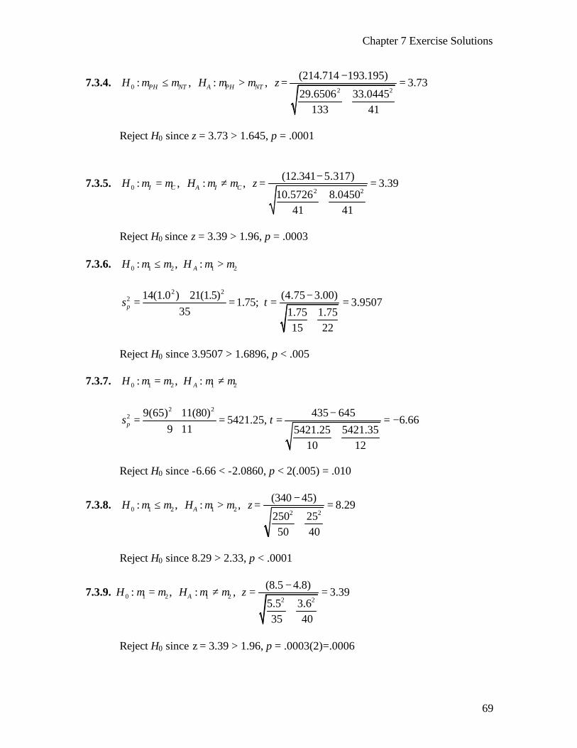
Chapter 7 Exercise Solutions
69
7.3.4. 0 2 2
(214.714 193.195): , : , 3.73
29.6506 33.0445133 41
PH NT A PH NTH H zµ µ µ µ−
≤ > = =
+
Reject H0 since z = 3.73 > 1.645, p = .0001
7.3.5. 0 2 2
(12.341 5.317): , : , 3.39
10.5726 8.045041 41
I C A I CH H zµ µ µ µ−
= ≠ = =
+
Reject H0 since z = 3.39 > 1.96, p = .0003
7.3.6. 0 1 2 1 2: , :AH Hµ µ µ µ≤ >
2 2
2 14(1.0 ) 21(1.5) (4.75 3.00)1.75; 3.9507
35 1.75 1.7515 22
ps t+ −
= = = =+
Reject H0 since 3.9507 > 1.6896, p < .005
7.3.7. 0 1 2 1 2: , :AH Hµ µ µ µ= ≠
2 22 9(65) 11(80) 435 645
5421.25, 6.669 11 5421.25 5421.35
10 12
ps t+ −
= = = = −+
+
Reject H0 since -6.66 < -2.0860, p < 2(.005) = .010
7.3.8. 0 1 2 1 2 2 2
(340 45): , : , 8.29
250 2550 40
AH H zµ µ µ µ−
≤ > = =
+
Reject H0 since 8.29 > 2.33, p < .0001
7.3.9. 0 1 2 1 2 2 2
(8.5 4.8): , : , 3.39
5.5 3.635 40
AH H zµ µ µ µ−
= ≠ = =
+
Reject H0 since z = 3.39 > 1.96, p = .0003(2)=.0006
Chapter 7 Exercise Solutions
70
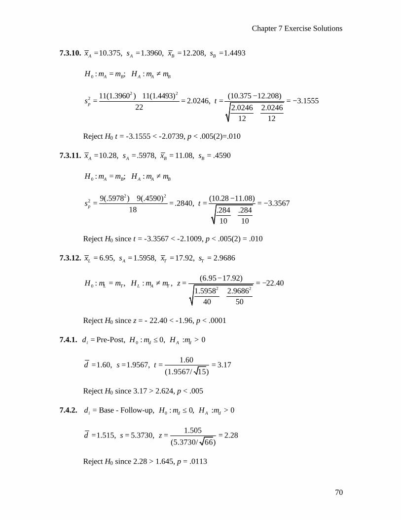
7.3.10. 10.375, 1.3960, 12.208, 1.4493A A B Bx s x s= = = = 0 : ; :A B A A BH Hµ µ µ µ= ≠
2 2
2 11(1.3960 ) 11(1.4493) (10.375 12.208)2.0246, 3.1555
22 2.0246 2.024612 12
ps t+ −
= = = = −+
Reject H0 t = -3.1555 < -2.0739, p < .005(2)=.010
7.3.11. 10.28, .5978, 11.08, .4590A A B Bx s x s= = = = 0 : ; :A B A A BH Hµ µ µ µ= ≠
2 2
2 9(.5978 ) 9(.4590) (10.28 11.08).2840, 3.3567
18 .284 .28410 10
ps t+ −
= = = = −+
Reject H0 since t = -3.3567 < -2.1009, p < .005(2) = .010
7.3.12. 6.95, 1.5958, 17.92, 2.9686L A T Tx s x s= = = =
0 2 2
(6.95 17.92): , : , 22.40
1.5958 2.968640 50
L T L A TH H zµ µ µ µ−
= ≠ = = −
+
Reject H0 since z = - 22.40 < -1.96, p < .0001
7.4.1. 0Pre-Post, : 0, : 0i d A dd H Hµ µ= ≤ >
1.60
1.60, 1.9567, 3.17(1.9567/ 15)
d s t= = = =
Reject H0 since 3.17 > 2.624, p < .005
7.4.2. 0Base - Follow-up, : 0, : 0i d A dd H Hµ µ= ≤ >
1.505
1.515, 5.3730, 2.28(5.3730/ 66)
d s z= = = =
Reject H0 since 2.28 > 1.645, p = .0113
Chapter 7 Exercise Solutions
71
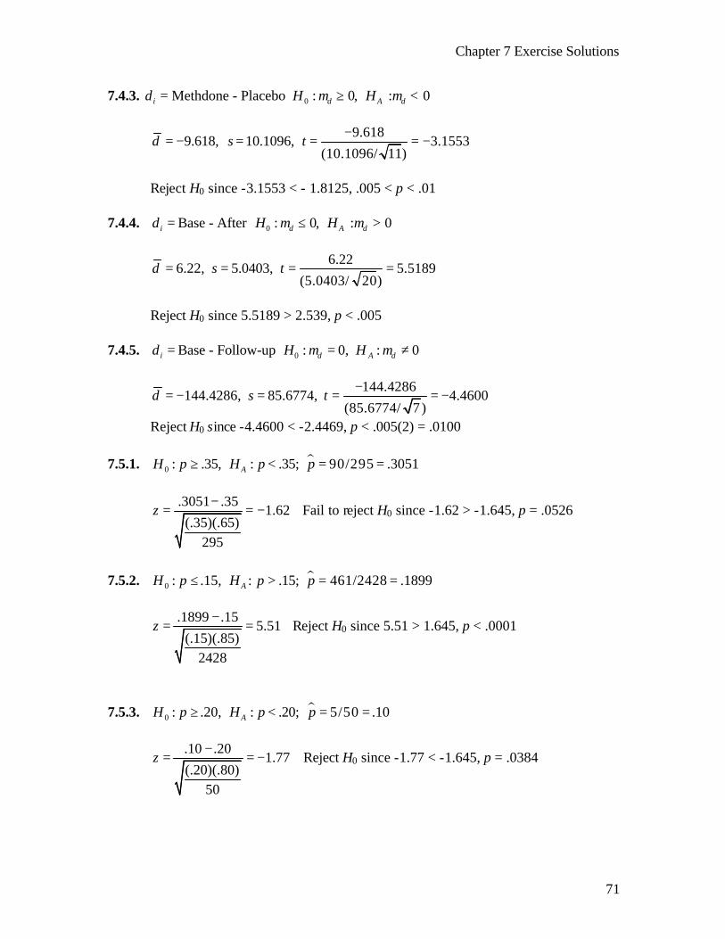
7.4.3. 0Methdone - Placebo : 0, : 0i d A dd H Hµ µ= ≥ <
9.618
9.618, 10.1096, 3.1553(10.1096/ 11)
d s t−
= − = = = −
Reject H0 since -3.1553 < - 1.8125, .005 < p < .01
7.4.4. 0Base - After : 0, : 0i d A dd H Hµ µ= ≤ >
6.22
6.22, 5.0403, 5.5189(5.0403/ 20)
d s t= = = =
Reject H0 since 5.5189 > 2.539, p < .005
7.4.5. 0Base - Follow-up : 0, : 0i d A dd H Hµ µ= = ≠
144.4286
144.4286, 85.6774, 4.4600(85.6774/ 7 )
d s t−
= − = = = −
Reject H0 since -4.4600 < -2.4469, p < .005(2) = .0100 7.5.1. µ
0 : .35, : .35; 90/295 .3051AH p H p p≥ < = =
.3051 .35
1.62(.35)(.65)
295
z−
= = − Fail to reject H0 since -1.62 > -1.645, p = .0526
7.5.2. µ0 : .15, : .15; 461/2428 .1899AH p H p p≤ > = =
.1899 .15
5.51(.15)(.85)
2428
z−
= = Reject H0 since 5.51 > 1.645, p < .0001
7.5.3. µ
0 : .20, : .20; 5/50 .10AH p H p p≥ < = =
.10 .20
1.77(.20)(.80)
50
z−
= = − Reject H0 since -1.77 < -1.645, p = .0384

Chapter 7 Exercise Solutions
72
7.5.4. µ0 : .60, : .60; 175/250 .70AH p H p p≤ > = =
.70 .60
3.23(.60)(.40)
250
z−
= = Reject H0 since 3.23 > 2.33, p = .0006
7.5.5. µ
0 : .15, : .15; 25/250 .10AH p H p p≥ < = =
.10 .15
2.21(.15)(.85)
250
z−
= = − Reject H0 since z= - 2.21 < -1.645, p = .0136
7.6.1. µ µ 72 3072/1222 .0589, 30/282 .1064, .0678
1222 282C Fp p p+
= = = = = =+
0
(.0589 .1064): , : , 2.86
.0678(.9322) .0678(.9322)1222 282
C F A C FH p p H p p z−
= ≠ = = −+
Reject H0 since -2.86 < - 2.58, p = .0042
7.6.2. µ µ 28 4328/175 .1600, 43/180 .2389, .2
175 180F Mp p p+
= = = = = =+
0
(.16 .2389): , : , 1.86
.2(.8) .2(.8)175 180
F M A F MH p p H p p z−
≥ < = = −+
Reject H0 since -1.86 < - 1.645, p = .0314
7.6.3. µ µ 249 134249/529 .4707, 134/326 .4110, .4480
529 326Hemo Perip p p+
= = = = = =+
0
(.4707 .4110): , : , 1.70
.4480(.5520) .4480(.5520)529 326
Hemo Peri A Hemo PeriH p p H p p z−
= ≠ = =+
Fail to reject H0 since 1.70 < 1.96, p = .0314(2) = .0628
Chapter 7 Exercise Solutions
73
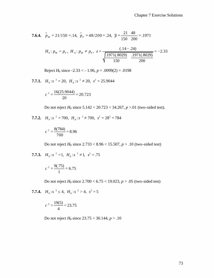
7.6.4. µ µ 21 4821/150 .14, 48/200 .24, .1971
150 200M Fp p p+
= = = = = =+
0
(.14 .24): , : , 2.33
.1971(.8029) .1971(.8029)150 200
M F A M FH p p H p p z−
= ≠ = = −+
Reject H0 since -2.33 < - 1.96, p = .0099(2) = .0198
7.7.1. 2 2 2
0 : 20, : 20, 25.9044AH H sσ σ= ≠ =
2 16(25.9044)20.723
20χ = =
Do not reject H0 since 5.142 < 20.723 < 34.267, p >.01 (two-sided test).
7.7.2. 2 2 2 2
0 : 700, : 700, 28 784AH H sσ σ= ≠ = =
2 8(784)8.96
700χ = =
Do not reject H0 since 2.733 < 8.96 < 15.507, p > .10 (two-sided test) 7.7.3. 2 2 2
0 : 1, : 1, .75AH H sσ σ= ≠ =
2 9(.75)6.75
1χ = =
Do not reject H0 since 2.700 < 6.75 < 19.023, p > .05 (two-sided test)
7.7.4. 2 2 2
0 : 4, : 4, 5AH H sσ σ≤ > =
2 19(5)23.75
4χ = =
Do not reject H0 since 23.75 < 30.144, p > .10

Chapter 7 Exercise Solutions
74
7.7.5. 2 2 2
0 : 25, : 25, 30AH H sσ σ≤ > =
2 24(30)28.8
25χ = =
Do not reject H0 since 28.8 < 36.415, p > .10
7.7.6. 2 2 2
0 : 250, : 250, 450AH H sσ σ≤ > =
2 14(450)25.20
250χ = =
Reject H0 since 25.20 > 23.685, .025 < p < .05
7.7.7. 2 2 2
0 : .05, : .05, .0787AH H sσ σ≤ > =
2 14(.0787)22.036
.05χ = =
Do not reject H0 since 22.036 < 23.685, .05 < p < .10
7.8.1. 2 2 2 2 2 2 2 2
0 : : , 3.1 9.61, 2.8 7.84, 30, 45D C A D C D C D CH H s s n nσ σ σ σ≤ > = = = = = =
9.61
V.R. = 1.2267.84
=
Fail to reject H0 since V.R. = 1.226 < 1.74, p > .10
7.8.2. 2 2 2 2
0 : :NMI MI A NMI MIH Hσ σ σ σ≤ > 2 2 2 211.6 134.56, 4.7 22.09, 42, 8NMI MI NMI MIs s n n= = = = = =
134.56
V.R. = 6.0922.09
=
Reject H0 since V.R. = 6.09 > 3.34, .005< p < .01
Chapter 7 Exercise Solutions
75
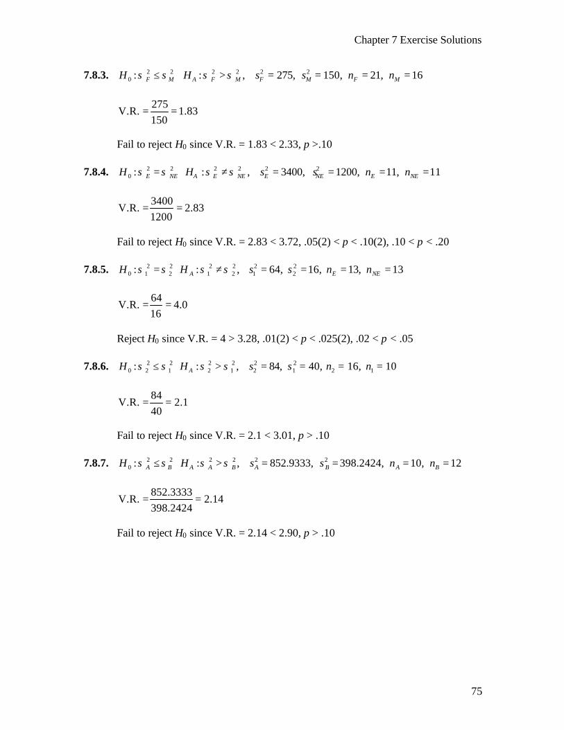
7.8.3. 2 2 2 20 : : ,F M A F MH Hσ σ σ σ≤ > 2 2275, 150, 21, 16F M F Ms s n n= = = =
275
V.R. = 1.83150
=
Fail to reject H0 since V.R. = 1.83 < 2.33, p >.10
7.8.4. 2 2 2 2
0 : : ,E NE A E NEH Hσ σ σ σ= ≠ 2 23400, 1200, 11, 11E NE E NEs s n n= = = =
3400
V.R. = 2.831200
=
Fail to reject H0 since V.R. = 2.83 < 3.72, .05(2) < p < .10(2), .10 < p < .20
7.8.5. 2 2 2 2
0 1 2 1 2: : ,AH Hσ σ σ σ= ≠ 2 21 264, 16, 13, 13E NEs s n n= = = =
64
V.R. = 4.016
=
Reject H0 since V.R. = 4 > 3.28, .01(2) < p < .025(2), .02 < p < .05
7.8.6. 2 2 2 2
0 2 1 2 1: : ,AH Hσ σ σ σ≤ > 2 22 1 2 184, 40, 16, 10s s n n= = = =
84
V.R. = 2.140
=
Fail to reject H0 since V.R. = 2.1 < 3.01, p > .10
7.8.7. 2 2 2 2
0 : : ,A B A A BH Hσ σ σ σ≤ > 2 2852.9333, 398.2424, 10, 12A B A Bs s n n= = = =
852.3333
V.R. = 2.14398.2424
=
Fail to reject H0 since V.R. = 2.14 < 2.90, p > .10

Chapter 7 Exercise Solutions
76
7.9.1.
Alternative Value of µ
β Value of Power Function 1- β
516 0.9500 0.0500 521 0.8461 0.1539 528 0.5596 0.4404 533 0.3156 0.6844 539 0.1093 0.8907 544 0.0314 0.9686 547 0.0129 0.9871
Alteranative values of mu
Pow
er
515 520 525 530 535 540 545
0.2
0.4
0.6
0.8
1.0

Chapter 7 Exercise Solutions
77
7.9.2.
Alternative Value of µ β Value of Power Function
1 β− 2.60 ≅.0207 ≅.9793 2.65 ≅.0619 ≅.9382 2.70 ≅.1492 ≅.8508 2.80 ≅.4840 ≅.5160 2.90 .8300 .1700 3.00 .9500 .0500 3.10 .8300 .1700 3.20 ≅.4840 ≅.5160 3.30 ≅.1492 ≅.8508 3.35 ≅.0618 ≅.9382 3.40 ≅.0207 ≅.9793
Alteranative values of mu
Pow
er
2.6 2.8 3.0 3.2 3.4
0.0
0.2
0.4
0.6
0.8
1.0
Chapter 7 Exercise Solutions
78
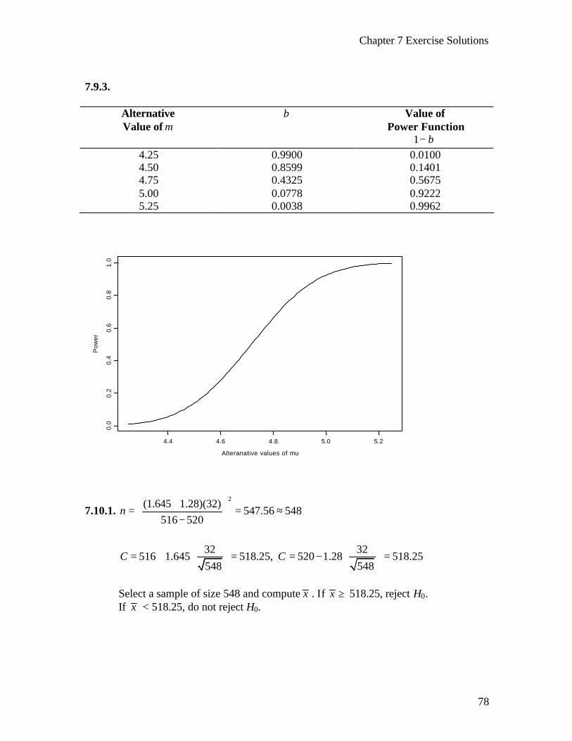
7.9.3.
Alternative Value of µ
β Value of Power Function
1 β− 4.25 0.9900 0.0100 4.50 0.8599 0.1401 4.75 0.4325 0.5675 5.00 0.0778 0.9222 5.25 0.0038 0.9962
Alteranative values of mu
Pow
er
4.4 4.6 4.8 5.0 5.2
0.0
0.2
0.4
0.6
0.8
1.0
7.10.1. 2(1.645 1.28)(32)
547.56 548516 520
n+ = = ≈ −
32 32
516 1.645 518.25, 520 1.28 518.25548 548
C C
= + = = − =
Select a sample of size 548 and compute x . If x ≥ 518.25, reject H0. If x < 518.25, do not reject H0.
Chapter 7 Exercise Solutions
79
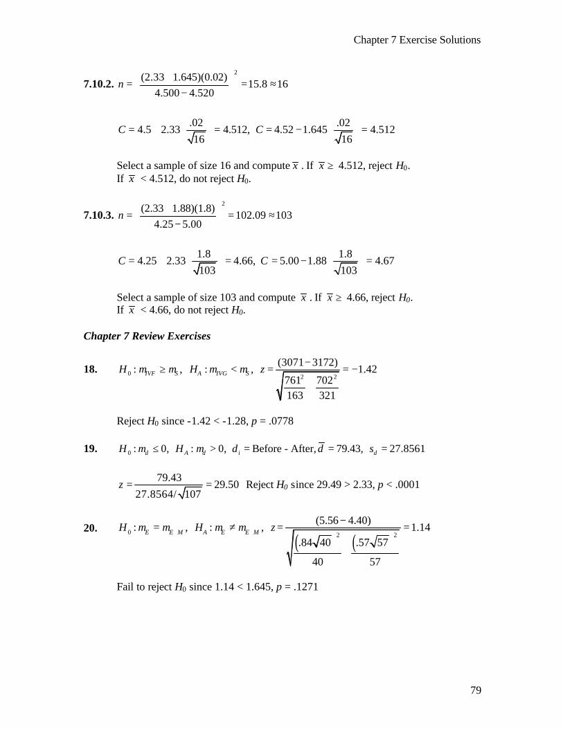
7.10.2. 2(2.33 1.645)(0.02)
15.8 164.500 4.520
n+ = = ≈ −
.02 .02
4.5 2.33 4.512, 4.52 1.645 4.51216 16
C C
= + = = − =
Select a sample of size 16 and compute x . If x ≥ 4.512, reject H0. If x < 4.512, do not reject H0.
7.10.3. 2(2.33 1.88)(1.8)
102.09 1034.25 5.00
n+ = = ≈ −
1.8 1.8
4.25 2.33 4.66, 5.00 1.88 4.67103 103
C C
= + = = − =
Select a sample of size 103 and compute x . If x ≥ 4.66, reject H0. If x < 4.66, do not reject H0.
Chapter 7 Review Exercises
18. 0 2 2
(3071 3172): , : , 1.42
761 702163 321
IVF S A IVG SH H zµ µ µ µ−
≥ < = = −
+
Reject H0 since -1.42 < -1.28, p = .0778 19. 0 : 0, : 0, Before - After, 79.43, 27.8561d A d i dH H d d sµ µ≤ > = = =
79.43
29.5027.8564/ 107
z = = Reject H0 since 29.49 > 2.33, p < .0001
20. ( ) ( )
0 2 2
(5.56 4.40): , : , 1.14
.84 40 .57 57
40 57
E E M A E E MH H zµ µ µ µ+ +
−= ≠ = =
+
Fail to reject H0 since 1.14 < 1.645, p = .1271
Chapter 7 Exercise Solutions
80
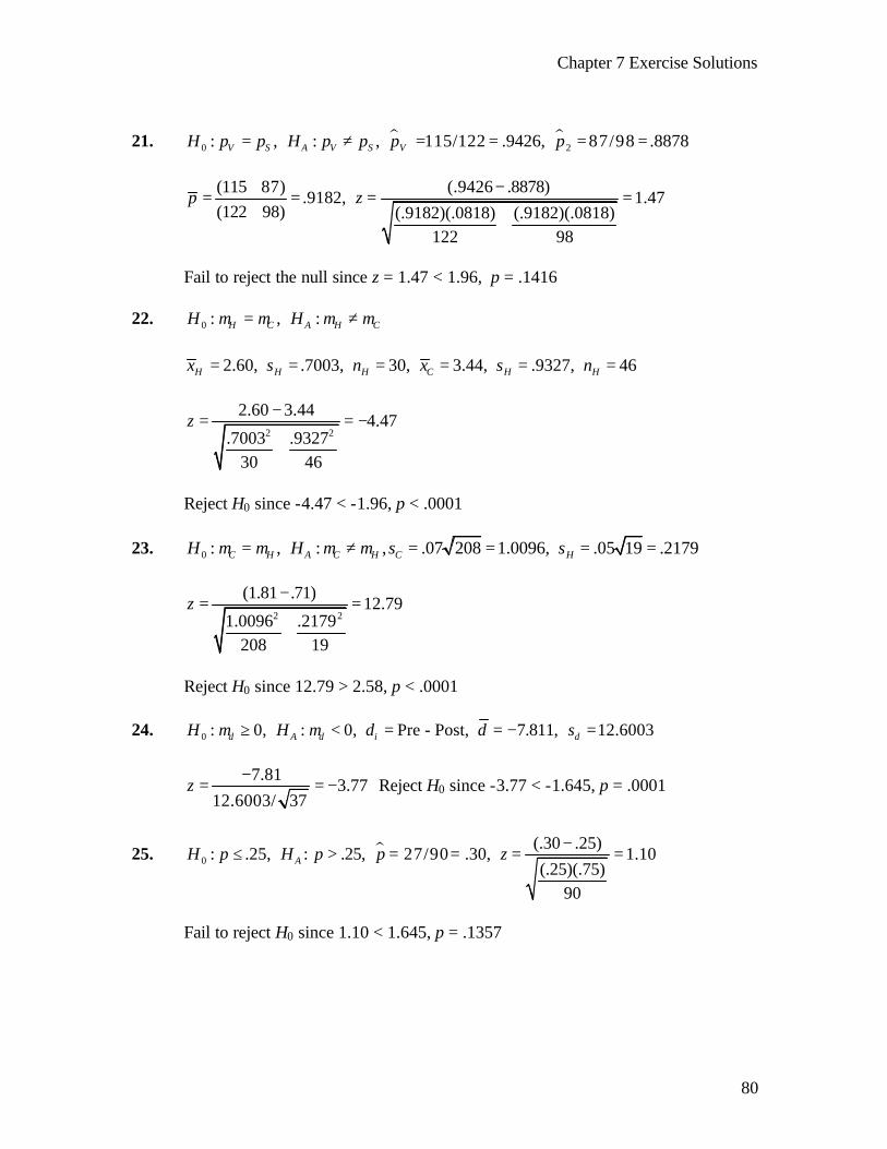
21. µ µ
0 2: , : , 115/122 .9426, 87/98 .8878V S A V S VH p p H p p p p= ≠ = = = =
(115 87) (.9426 .8878)
.9182, 1.47(122 98) (.9182)(.0818) (.9182)(.0818)
122 98
p z+ −
= = = =+
+
Fail to reject the null since z = 1.47 < 1.96, p = .1416
22. 0 : , :H C A H CH Hµ µ µ µ= ≠ 2.60, .7003, 30, 3.44, .9327, 46H H H C H Hx s n x s n= = = = = =
2 2
2.60 3.444.47
.7003 .932730 46
z−
= = −
+
Reject H0 since -4.47 < -1.96, p < .0001 23. 0 : , : , .07 208 1.0096, .05 19 .2179C H A C H C HH H s sµ µ µ µ= ≠ = = = =
2 2
(1.81 .71)12.79
1.0096 .2179208 19
z−
= =
+
Reject H0 since 12.79 > 2.58, p < .0001
24. 0 : 0, : 0, Pre - Post, 7.811, 12.6003d A d i dH H d d sµ µ≥ < = = − =
7.81
3.7712.6003/ 37
z−
= = − Reject H0 since -3.77 < -1.645, p = .0001
25. µ0
(.30 .25): .25, : .25, 27/90 .30, 1.10
(.25)(.75)90
AH p H p p z−
≤ > = = = =
Fail to reject H0 since 1.10 < 1.645, p = .1357
Chapter 7 Exercise Solutions
81
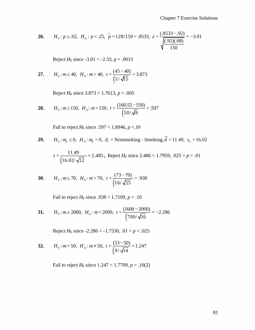
26. µ0
(.8533 .92): .02, : .25, 128/150 .8533, 3.01
(.92)(.08)150
AH p H p p z−
≥ < = = = = −
Reject H0 since -3.01 < -2.33, p = .0013
27. ( )0
(45 40): 40, : 40, 3.873
5 / 15AH H tµ µ
−≤ > = =
Reject H0 since 3.873 > 1.7613, p < .005
28. ( )0
(160.55 150): 150, : 150, .597
50/ 8AH H tµ µ
−≤ > = =
Fail to reject H0 since .597 < 1.8946, p <.10
29. 0 : 0, : 0, Nonsmoking - Smoking, 11.49, 16.02d A d i dH H d d sµ µ≤ > = = =
( )
11.492.485
16.02/ 12t = = , Reject H0 since 2.486 > 1.7959, .025 > p > .01
30. ( )0
(73 70): 70, : 70, .938
16/ 25AH H tµ µ
−≤ > = =
Fail to reject H0 since .938 < 1.7109, p > .10
31. ( )0
(1600 2000): 2000, : 2000, 2.286
700/ 16AH H tµ µ
−≥ < = = −
Reject H0 since -2.286 < -1.7530, .01 < p < .025
32. ( )0
(53 50): 50, : 50, 1.247
9 / 14AH H tµ µ
−= ≠ = =
Fail to reject H0 since 1.247 < 1.7709, p > .10(2)
Chapter 7 Exercise Solutions
82
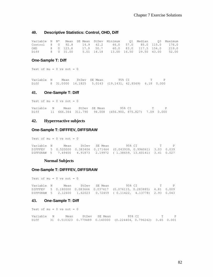
40. Descriptive Statistics: Control, OHD, Diff Variable N N* Mean SE Mean StDev Minimum Q1 Median Q3 Maximum Control 8 0 92.8 14.9 42.2 46.0 57.0 85.0 115.0 176.0 OHD 8 0 123.8 17.9 50.7 60.0 83.0 117.5 154.0 219.0 Diff 8 0 31.00 5.01 14.18 13.00 16.50 29.50 43.00 52.00 One-Sample T: Diff Test of mu = 0 vs not = 0 Variable N Mean StDev SE Mean 95% CI T P Diff 8 31.0000 14.1825 5.0143 (19.1431, 42.8569) 6.18 0.000 41. One-Sample T: Diff Test of mu = 0 vs not = 0 Variable N Mean StDev SE Mean 95% CI T P Diff 11 666.364 311.790 94.008 (456.900, 875.827) 7.09 0.000 42. Hyperreactive subjects One-Sample T: DIFFFEV, DIFFSRAW Test of mu = 0 vs not = 0 Variable N Mean StDev SE Mean 95% CI T P DIFFFEV 5 0.520000 0.383406 0.171464 (0.043939, 0.996061) 3.03 0.039 DIFFSRAW 5 7.49400 4.91873 2.19972 ( 1.38659, 13.60141) 3.41 0.027
Normal Subjects
One-Sample T: DIFFFEV, DIFFSRAW Test of mu = 0 vs not = 0 Variable N Mean StDev SE Mean 95% CI T P DIFFFEV 5 0.180000 0.083666 0.037417 (0.076115, 0.283885) 4.81 0.009 DIFFSRAW 5 2.12600 1.62023 0.72459 ( 0.11422, 4.13778) 2.93 0.043 43. One-Sample T: Diff Test of mu = 0 vs not = 0 Variable N Mean StDev SE Mean 95% CI T P Diff 31 0.510323 0.779489 0.140000 (0.224404, 0.796242) 3.65 0.001
Chapter 7 Exercise Solutions
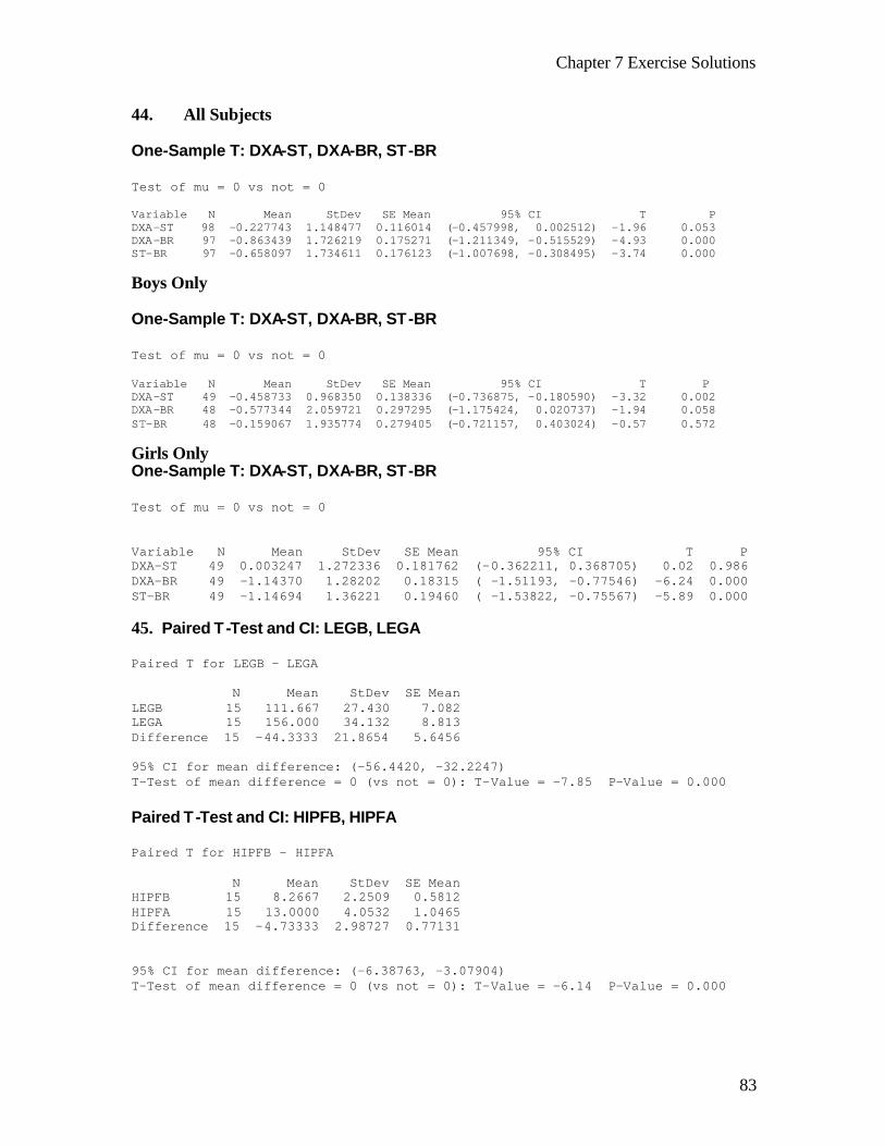
83
44. All Subjects One-Sample T: DXA-ST, DXA-BR, ST-BR Test of mu = 0 vs not = 0 Variable N Mean StDev SE Mean 95% CI T P DXA-ST 98 -0.227743 1.148477 0.116014 (-0.457998, 0.002512) -1.96 0.053 DXA-BR 97 -0.863439 1.726219 0.175271 (-1.211349, -0.515529) -4.93 0.000 ST-BR 97 -0.658097 1.734611 0.176123 (-1.007698, -0.308495) -3.74 0.000 Boys Only One-Sample T: DXA-ST, DXA-BR, ST-BR Test of mu = 0 vs not = 0 Variable N Mean StDev SE Mean 95% CI T P DXA-ST 49 -0.458733 0.968350 0.138336 (-0.736875, -0.180590) -3.32 0.002 DXA-BR 48 -0.577344 2.059721 0.297295 (-1.175424, 0.020737) -1.94 0.058 ST-BR 48 -0.159067 1.935774 0.279405 (-0.721157, 0.403024) -0.57 0.572 Girls Only One-Sample T: DXA-ST, DXA-BR, ST-BR Test of mu = 0 vs not = 0 Variable N Mean StDev SE Mean 95% CI T P DXA-ST 49 0.003247 1.272336 0.181762 (-0.362211, 0.368705) 0.02 0.986 DXA-BR 49 -1.14370 1.28202 0.18315 ( -1.51193, -0.77546) -6.24 0.000 ST-BR 49 -1.14694 1.36221 0.19460 ( -1.53822, -0.75567) -5.89 0.000 45. Paired T-Test and CI: LEGB, LEGA Paired T for LEGB - LEGA N Mean StDev SE Mean LEGB 15 111.667 27.430 7.082 LEGA 15 156.000 34.132 8.813 Difference 15 -44.3333 21.8654 5.6456 95% CI for mean difference: (-56.4420, -32.2247) T-Test of mean difference = 0 (vs not = 0): T-Value = -7.85 P-Value = 0.000 Paired T-Test and CI: HIPFB, HIPFA Paired T for HIPFB - HIPFA N Mean StDev SE Mean HIPFB 15 8.2667 2.2509 0.5812 HIPFA 15 13.0000 4.0532 1.0465 Difference 15 -4.73333 2.98727 0.77131 95% CI for mean difference: (-6.38763, -3.07904) T-Test of mean difference = 0 (vs not = 0): T-Value = -6.14 P-Value = 0.000
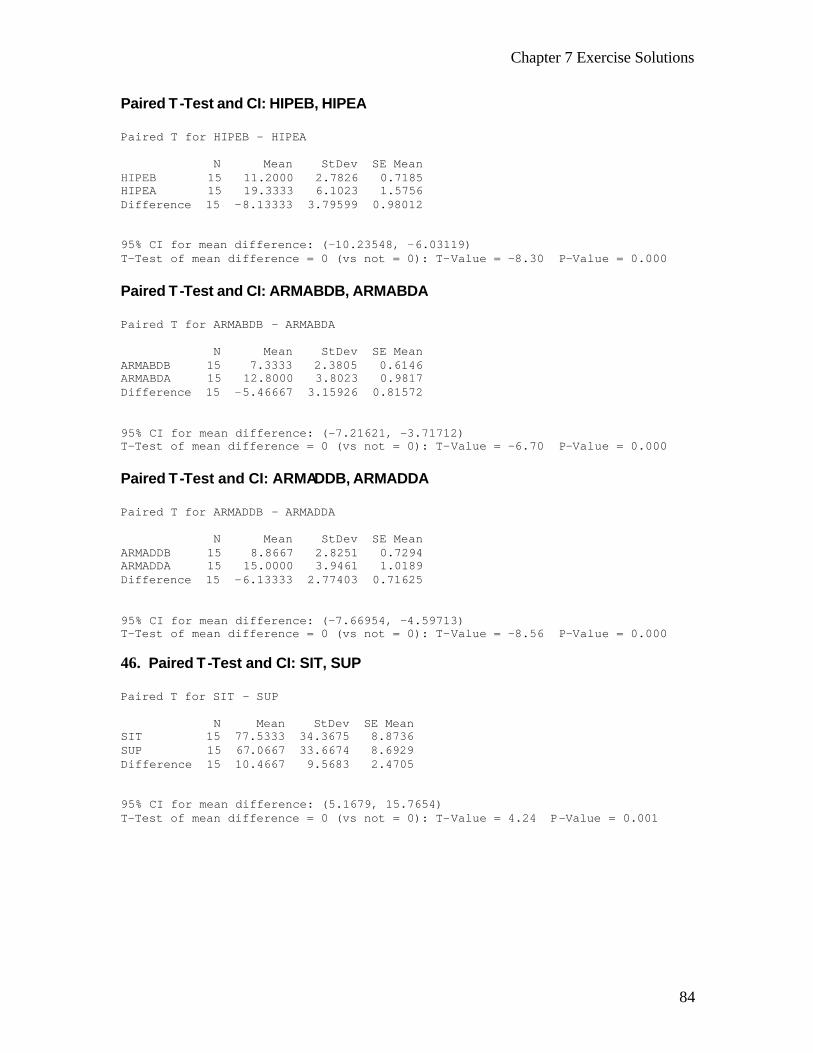
Chapter 7 Exercise Solutions
84
Paired T-Test and CI: HIPEB, HIPEA Paired T for HIPEB - HIPEA N Mean StDev SE Mean HIPEB 15 11.2000 2.7826 0.7185 HIPEA 15 19.3333 6.1023 1.5756 Difference 15 -8.13333 3.79599 0.98012 95% CI for mean difference: (-10.23548, -6.03119) T-Test of mean difference = 0 (vs not = 0): T-Value = -8.30 P-Value = 0.000 Paired T-Test and CI: ARMABDB, ARMABDA Paired T for ARMABDB - ARMABDA N Mean StDev SE Mean ARMABDB 15 7.3333 2.3805 0.6146 ARMABDA 15 12.8000 3.8023 0.9817 Difference 15 -5.46667 3.15926 0.81572 95% CI for mean difference: (-7.21621, -3.71712) T-Test of mean difference = 0 (vs not = 0): T-Value = -6.70 P-Value = 0.000 Paired T-Test and CI: ARMADDB, ARMADDA Paired T for ARMADDB - ARMADDA N Mean StDev SE Mean ARMADDB 15 8.8667 2.8251 0.7294 ARMADDA 15 15.0000 3.9461 1.0189 Difference 15 -6.13333 2.77403 0.71625 95% CI for mean difference: (-7.66954, -4.59713) T-Test of mean difference = 0 (vs not = 0): T-Value = -8.56 P-Value = 0.000 46. Paired T-Test and CI: SIT, SUP Paired T for SIT - SUP N Mean StDev SE Mean SIT 15 77.5333 34.3675 8.8736 SUP 15 67.0667 33.6674 8.6929 Difference 15 10.4667 9.5683 2.4705 95% CI for mean difference: (5.1679, 15.7654) T-Test of mean difference = 0 (vs not = 0): T-Value = 4.24 P-Value = 0.001

Chapter 7 Exercise Solutions
85
47. Paired T-Test and CI: PRE, POST Paired T for PRE - POST N Mean StDev SE Mean PRE 66 392.439 125.950 15.503 POST 66 343.242 105.432 12.978 Difference 66 49.1970 92.1966 11.3486 95% CI for mean difference: (26.5322, 71.8617) T-Test of mean difference = 0 (vs not = 0): T-Value = 4.34 P-Value = 0.000 48. Paired T-Test and CI: ADM, DIS Paired T for ADM - DIS N Mean StDev SE Mean ADM 51 22.6078 5.3817 0.7536 DIS 51 23.4902 5.3940 0.7553 Difference 51 -0.882353 2.150786 0.301170 95% CI for mean difference: (-1.487271, -0.277435) T-Test of mean difference = 0 (vs not = 0): T-Value = -2.93 P-Value = 0.005 49. Two-Sample T-Test and CI: NOASTH, ASTH Two-sample T for NOASTH vs ASTH N Mean StDev SE Mean NOASTH 22 56.1 43.0 9.2 ASTH 22 108.0 60.0 13 Difference = mu (NOASTH) - mu (ASTH) Estimate for difference: -51.8977 95% CI for difference: (-83.6549, -20.1405) T-Test of difference = 0 (vs not =): T-Value = -3.30 P-Value = 0.002 DF = 42 Both use Pooled StDev = 52.1915
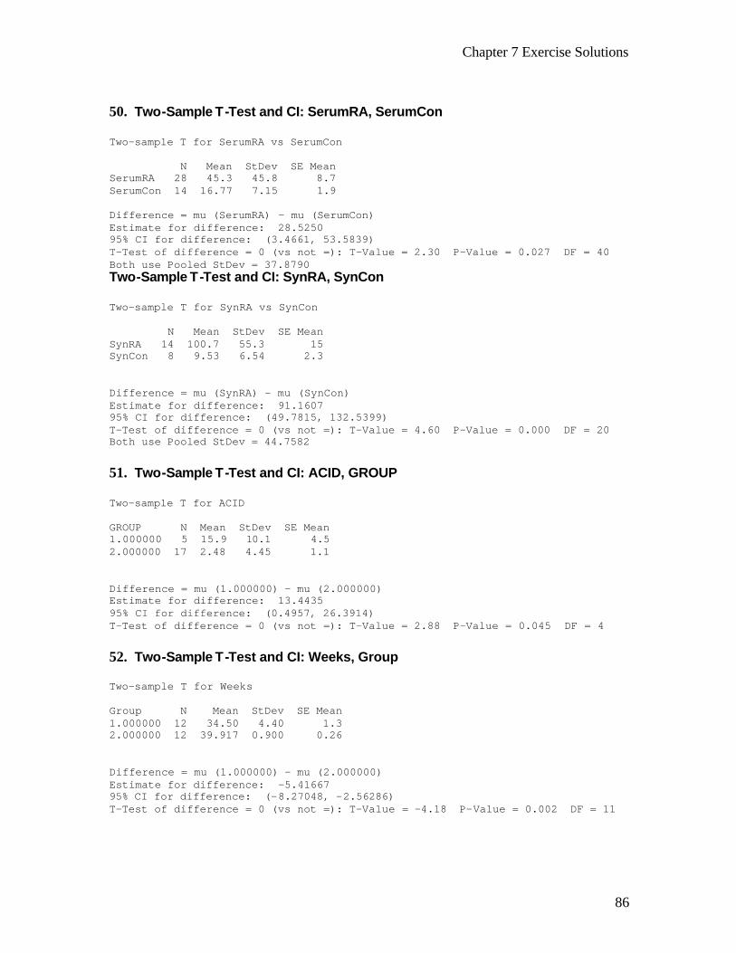
Chapter 7 Exercise Solutions
86
50. Two-Sample T-Test and CI: SerumRA, SerumCon Two-sample T for SerumRA vs SerumCon N Mean StDev SE Mean SerumRA 28 45.3 45.8 8.7 SerumCon 14 16.77 7.15 1.9 Difference = mu (SerumRA) - mu (SerumCon) Estimate for difference: 28.5250 95% CI for difference: (3.4661, 53.5839) T-Test of difference = 0 (vs not =): T-Value = 2.30 P-Value = 0.027 DF = 40 Both use Pooled StDev = 37.8790 Two-Sample T-Test and CI: SynRA, SynCon Two-sample T for SynRA vs SynCon N Mean StDev SE Mean SynRA 14 100.7 55.3 15 SynCon 8 9.53 6.54 2.3 Difference = mu (SynRA) - mu (SynCon) Estimate for difference: 91.1607 95% CI for difference: (49.7815, 132.5399) T-Test of difference = 0 (vs not =): T-Value = 4.60 P-Value = 0.000 DF = 20 Both use Pooled StDev = 44.7582 51. Two-Sample T-Test and CI: ACID, GROUP Two-sample T for ACID GROUP N Mean StDev SE Mean 1.000000 5 15.9 10.1 4.5 2.000000 17 2.48 4.45 1.1 Difference = mu (1.000000) - mu (2.000000) Estimate for difference: 13.4435 95% CI for difference: (0.4957, 26.3914) T-Test of difference = 0 (vs not =): T-Value = 2.88 P-Value = 0.045 DF = 4 52. Two-Sample T-Test and CI: Weeks, Group Two-sample T for Weeks Group N Mean StDev SE Mean 1.000000 12 34.50 4.40 1.3 2.000000 12 39.917 0.900 0.26 Difference = mu (1.000000) - mu (2.000000) Estimate for difference: -5.41667 95% CI for difference: (-8.27048, -2.56286) T-Test of difference = 0 (vs not =): T-Value = -4.18 P-Value = 0.002 DF = 11
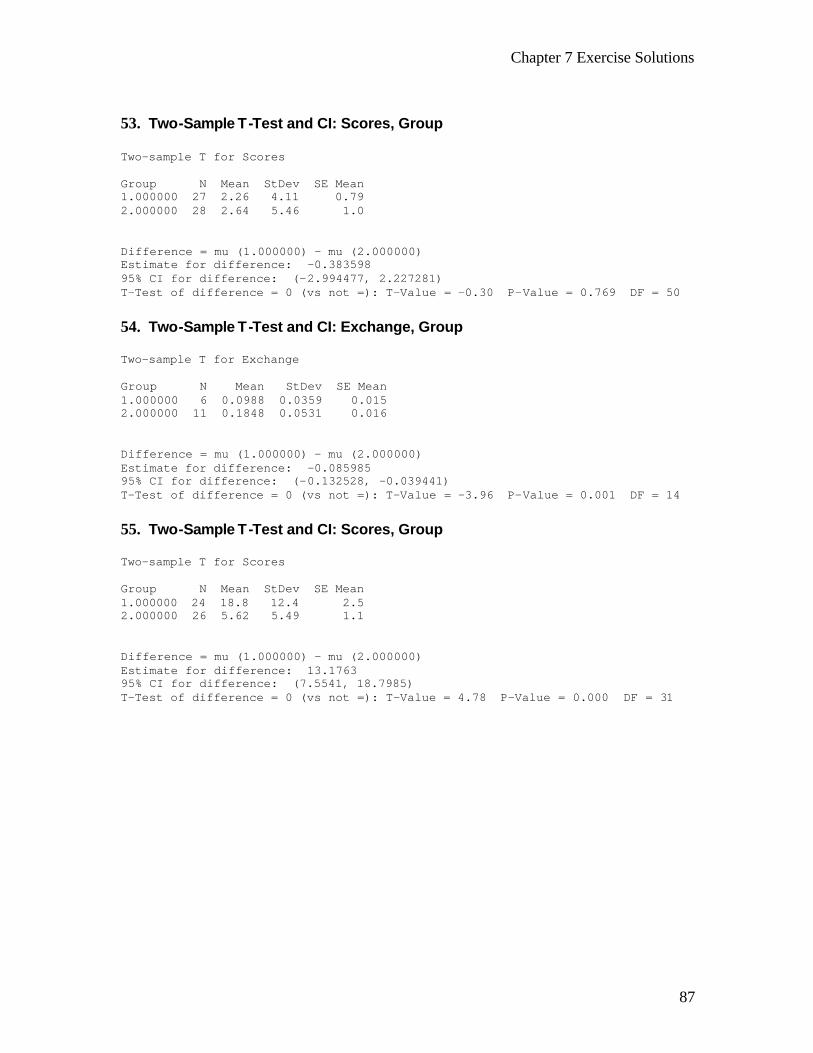
Chapter 7 Exercise Solutions
87
53. Two-Sample T-Test and CI: Scores, Group Two-sample T for Scores Group N Mean StDev SE Mean 1.000000 27 2.26 4.11 0.79 2.000000 28 2.64 5.46 1.0 Difference = mu (1.000000) - mu (2.000000) Estimate for difference: -0.383598 95% CI for difference: (-2.994477, 2.227281) T-Test of difference = 0 (vs not =): T-Value = -0.30 P-Value = 0.769 DF = 50 54. Two-Sample T-Test and CI: Exchange, Group Two-sample T for Exchange Group N Mean StDev SE Mean 1.000000 6 0.0988 0.0359 0.015 2.000000 11 0.1848 0.0531 0.016 Difference = mu (1.000000) - mu (2.000000) Estimate for difference: -0.085985 95% CI for difference: (-0.132528, -0.039441) T-Test of difference = 0 (vs not =): T-Value = -3.96 P-Value = 0.001 DF = 14 55. Two-Sample T-Test and CI: Scores, Group Two-sample T for Scores Group N Mean StDev SE Mean 1.000000 24 18.8 12.4 2.5 2.000000 26 5.62 5.49 1.1 Difference = mu (1.000000) - mu (2.000000) Estimate for difference: 13.1763 95% CI for difference: (7.5541, 18.7985) T-Test of difference = 0 (vs not =): T-Value = 4.78 P-Value = 0.000 DF = 31

Chapter 8 Exercise Solutions
88
Chapter 8 Answers for 8.2.1-8.2.7 obtained by SAS® 8.2.1. The MEANS Procedure Analysis Variable : EMT N ANGLE Obs N Mean Std Dev Minimum Maximum ƒƒƒƒƒƒƒƒƒƒƒƒƒƒƒƒƒƒƒƒƒƒƒƒƒƒƒƒƒƒƒƒƒƒƒƒƒƒƒƒƒƒƒƒƒƒƒƒƒƒƒƒƒƒƒƒƒƒƒƒƒƒƒƒƒƒƒƒƒƒƒƒƒƒƒƒƒƒƒƒƒƒƒƒƒƒƒƒƒƒ 30 69 69 0.6877391 0.7975196 -1.1640000 2.7330000 60 33 33 0.2401515 0.9769852 -1.1890000 2.7270000 90 194 194 0.8787990 1.1203785 -2.8620000 2.7620000 120 33 33 0.2441818 0.9867145 -1.1800000 2.7630000 Dependent Variable: EMT Sum of Source DF Squares Mean Square F Value Pr > F Model 3 20.0070713 6.6690238 6.24 0.0004 Error 325 347.2127836 1.0683470 Corrected Total 328 367.2198549
30,60 .05,4,3251.608347 1 1
* 3.65207*.1897988 .69312 69 33
HSD q = + = =
Since 30 60.6877 .2402 .4475 .6931, x x− = < − is not significant.
30,90 .05,4,3251.608347 1 1
* 3.65207*.1256878 .45912 69 194
HSD q = + = =
Since 30 90.6877 .8788 .1911 .6931, x x− = < − is not significant.
30,120 .05,4,3251.608347 1 1
* 3.65207*.1897988 .69312 69 33
HSD q = + = =
Since 30 60.6877 .2442 .4435 .6931, x x− = < − is not significant.
60,90 .05,4,3251.608347 1 1
* 3.65207*.16886 .61672 33 194
HSD q = + = =
Since 60 90.2402 .8788 .6386 .6137, x x− = > − is significant.

Chapter 8 Exercise Solutions
89
60,120 .05,4,3251.608347 1 1
* 3.65207*.22077 .80632 33 33
HSD q = + = =
Since 60 120.2402 .2442 .0004 .8063, x x− = < − is not significant.
90,120 .05,4,3251.608347 1 1
* 3.65207*.16886 .61672 194 33
HSD q = + = =
Since 90 120.8788 .2442 .6346 .6167,x x− = > − is significant.
Alpha 0.05 Error Degrees of Freedom 325 Error Mean Square 1.068347 Critical Value of Studentized Range 3.65207 Comparisons significant at the 0.05 level are indicated by ***. Difference Simultaneous group Between 95% Confidence Comparison Means Limits 90 - 30 0.1911 -0.1831 0.5652 90 -120 0.6346 0.1320 1.1372 *** 90 - 60 0.6386 0.1360 1.1413 *** 30 - 90 -0.1911 -0.5652 0.1831 30 -120 0.4436 -0.1214 1.0085 30 - 60 0.4476 -0.1173 1.0125 120 - 90 -0.6346 -1.1372 -0.1320 *** 120 - 30 -0.4436 -1.0085 0.1214 120 - 60 0.0040 -0.6531 0.6611 60 - 90 -0.6386 -1.1413 -0.1360 *** 60 - 30 -0.4476 -1.0125 0.1173 60 -120 -0.0040 -0.6611 0.6531
8.2.2. Analysis Variable : BMD N GROUP Obs N Mean Std Dev Minimum Maximum ƒƒƒƒƒƒƒƒƒƒƒƒƒƒƒƒƒƒƒƒƒƒƒƒƒƒƒƒƒƒƒƒƒƒƒƒƒƒƒƒƒƒƒƒƒƒƒƒƒƒƒƒƒƒƒƒƒƒƒƒƒƒƒƒƒƒƒƒƒƒƒƒƒƒƒƒƒƒƒƒƒƒƒƒƒƒƒƒƒ 1 37 37 4.4698919 7.4991601 -9.6460000 24.4140000 2 9 9 4.5780000 3.9913172 -1.3690000 11.2880000 3 16 16 2.1808125 4.5425362 -7.8160000 10.7340000 4 24 24 5.2045417 4.6216400 -2.8170000 15.8530000 5 10 10 9.6718000 8.1538216 1.7190000 25.6550000
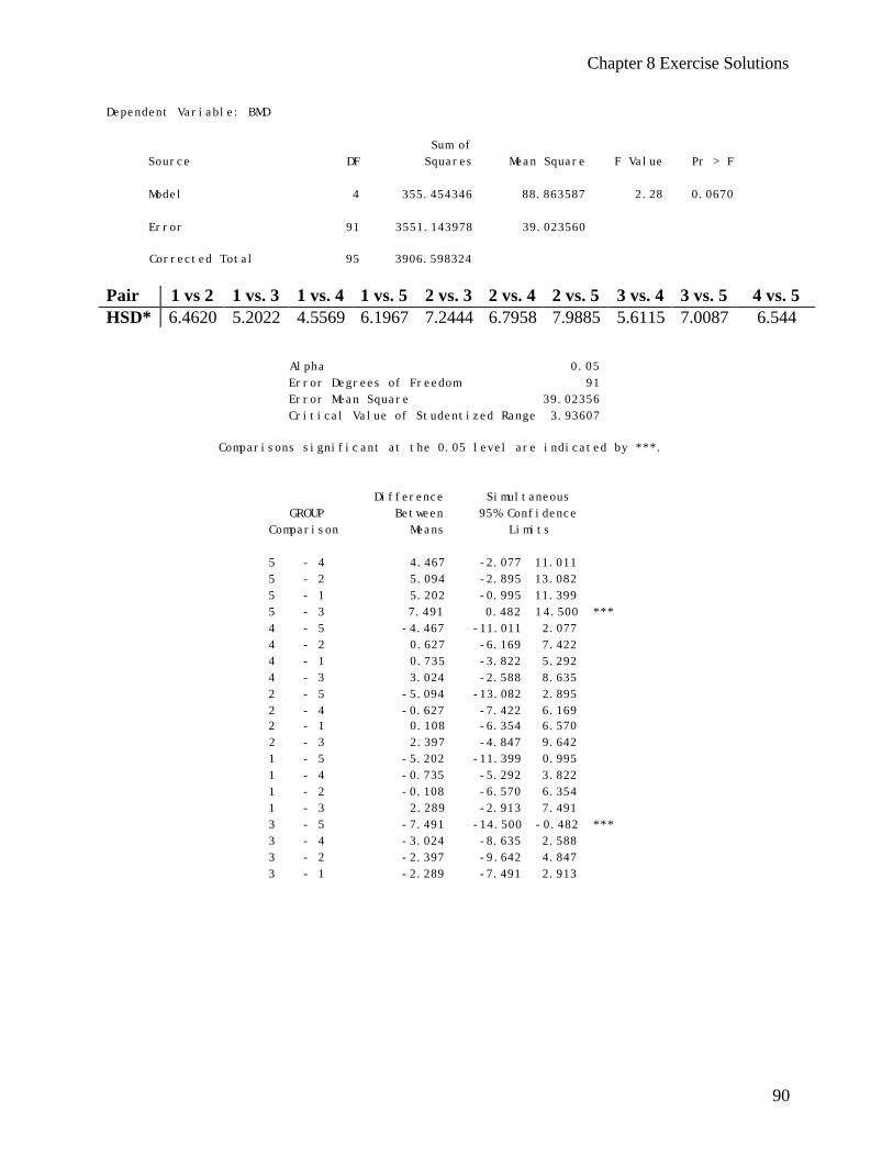
Chapter 8 Exercise Solutions
90
Dependent Variable: BMD Sum of Source DF Squares Mean Square F Value Pr > F Model 4 355.454346 88.863587 2.28 0.0670 Error 91 3551.143978 39.023560 Corrected Total 95 3906.598324
Pair 1 vs 2 1 vs. 3 1 vs. 4 1 vs. 5 2 vs. 3 2 vs. 4 2 vs. 5 3 vs. 4 3 vs. 5 4 vs. 5 HSD* 6.4620 5.2022 4.5569 6.1967 7.2444 6.7958 7.9885 5.6115 7.0087 6.544 Alpha 0.05 Error Degrees of Freedom 91 Error Mean Square 39.02356 Critical Value of Studentized Range 3.93607 Comparisons significant at the 0.05 level are indicated by ***. Difference Simultaneous GROUP Between 95% Confidence Comparison Means Limits 5 - 4 4.467 -2.077 11.011 5 - 2 5.094 -2.895 13.082 5 - 1 5.202 -0.995 11.399 5 - 3 7.491 0.482 14.500 *** 4 - 5 -4.467 -11.011 2.077 4 - 2 0.627 -6.169 7.422 4 - 1 0.735 -3.822 5.292 4 - 3 3.024 -2.588 8.635 2 - 5 -5.094 -13.082 2.895 2 - 4 -0.627 -7.422 6.169 2 - 1 0.108 -6.354 6.570 2 - 3 2.397 -4.847 9.642 1 - 5 -5.202 -11.399 0.995 1 - 4 -0.735 -5.292 3.822 1 - 2 -0.108 -6.570 6.354 1 - 3 2.289 -2.913 7.491 3 - 5 -7.491 -14.500 -0.482 *** 3 - 4 -3.024 -8.635 2.588 3 - 2 -2.397 -9.642 4.847 3 - 1 -2.289 -7.491 2.913
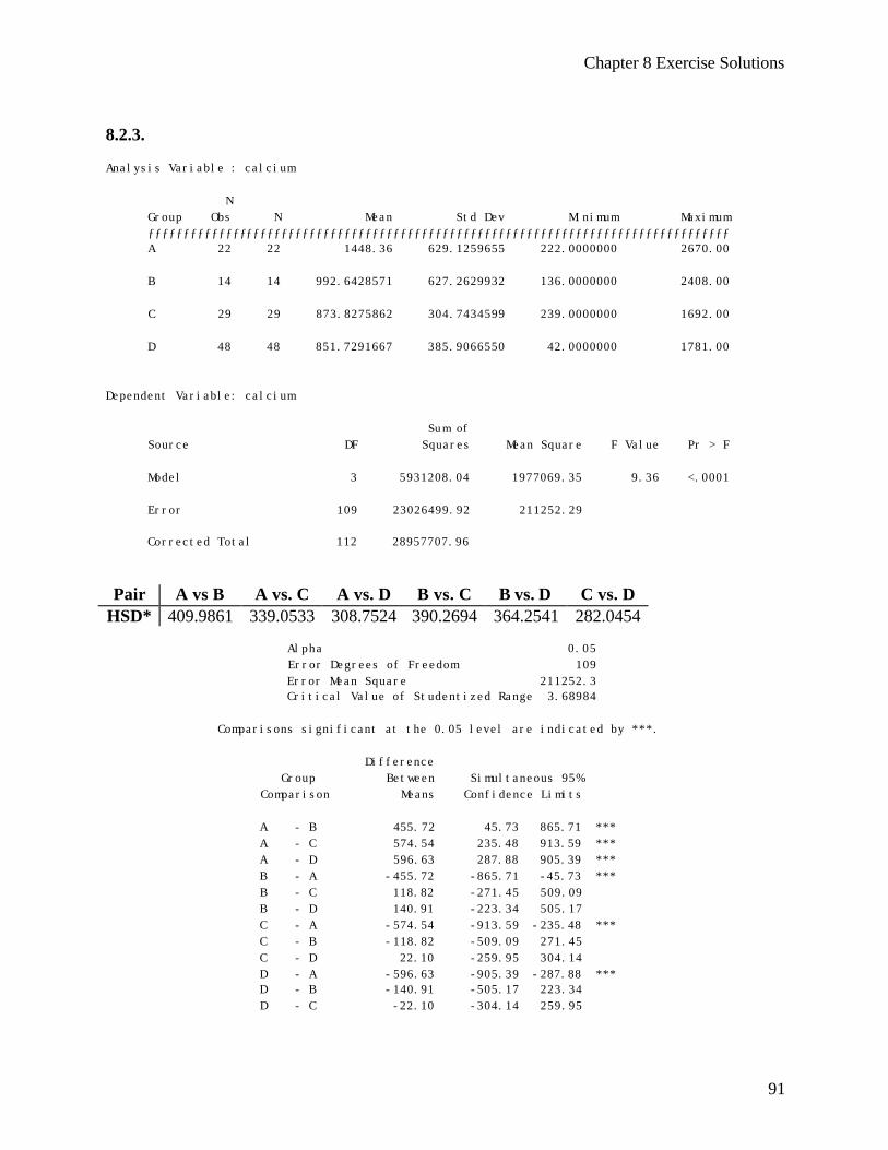
Chapter 8 Exercise Solutions
91
8.2.3. Analysis Variable : calcium N Group Obs N Mean Std Dev Minimum Maximum ƒƒƒƒƒƒƒƒƒƒƒƒƒƒƒƒƒƒƒƒƒƒƒƒƒƒƒƒƒƒƒƒƒƒƒƒƒƒƒƒƒƒƒƒƒƒƒƒƒƒƒƒƒƒƒƒƒƒƒƒƒƒƒƒƒƒƒƒƒƒƒƒƒƒƒƒƒƒƒƒƒƒƒ A 22 22 1448.36 629.1259655 222.0000000 2670.00 B 14 14 992.6428571 627.2629932 136.0000000 2408.00 C 29 29 873.8275862 304.7434599 239.0000000 1692.00 D 48 48 851.7291667 385.9066550 42.0000000 1781.00 Dependent Variable: calcium Sum of Source DF Squares Mean Square F Value Pr > F Model 3 5931208.04 1977069.35 9.36 <.0001 Error 109 23026499.92 211252.29 Corrected Total 112 28957707.96
Pair A vs B A vs. C A vs. D B vs. C B vs. D C vs. D HSD* 409.9861 339.0533 308.7524 390.2694 364.2541 282.0454 Alpha 0.05 Error Degrees of Freedom 109 Error Mean Square 211252.3 Critical Value of Studentized Range 3.68984 Comparisons significant at the 0.05 level are indicated by ***. Difference Group Between Simultaneous 95% Comparison Means Confidence Limits A - B 455.72 45.73 865.71 *** A - C 574.54 235.48 913.59 *** A - D 596.63 287.88 905.39 *** B - A -455.72 -865.71 -45.73 *** B - C 118.82 -271.45 509.09 B - D 140.91 -223.34 505.17 C - A -574.54 -913.59 -235.48 *** C - B -118.82 -509.09 271.45 C - D 22.10 -259.95 304.14 D - A -596.63 -905.39 -287.88 *** D - B -140.91 -505.17 223.34 D - C -22.10 -304.14 259.95
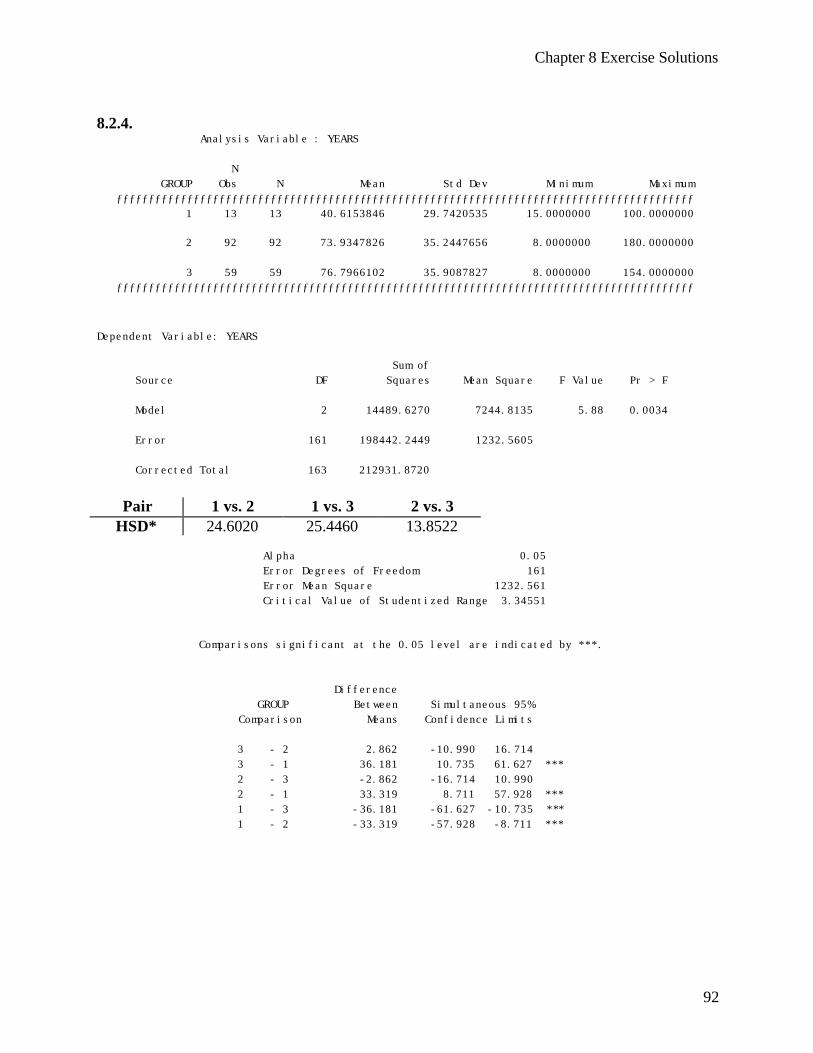
Chapter 8 Exercise Solutions
92
8.2.4. Analysis Variable : YEARS N GROUP Obs N Mean Std Dev Minimum Maximum ƒƒƒƒƒƒƒƒƒƒƒƒƒƒƒƒƒƒƒƒƒƒƒƒƒƒƒƒƒƒƒƒƒƒƒƒƒƒƒƒƒƒƒƒƒƒƒƒƒƒƒƒƒƒƒƒƒƒƒƒƒƒƒƒƒƒƒƒƒƒƒƒƒƒƒƒƒƒƒƒƒƒƒƒƒƒƒƒƒƒ 1 13 13 40.6153846 29.7420535 15.0000000 100.0000000 2 92 92 73.9347826 35.2447656 8.0000000 180.0000000 3 59 59 76.7966102 35.9087827 8.0000000 154.0000000 ƒƒƒƒƒƒƒƒƒƒƒƒƒƒƒƒƒƒƒƒƒƒƒƒƒƒƒƒƒƒƒƒƒƒƒƒƒƒƒƒƒƒƒƒƒƒƒƒƒƒƒƒƒƒƒƒƒƒƒƒƒƒƒƒƒƒƒƒƒƒƒƒƒƒƒƒƒƒƒƒƒƒƒƒƒƒƒƒƒƒ Dependent Variable: YEARS Sum of Source DF Squares Mean Square F Value Pr > F Model 2 14489.6270 7244.8135 5.88 0.0034 Error 161 198442.2449 1232.5605 Corrected Total 163 212931.8720
Pair 1 vs. 2 1 vs. 3 2 vs. 3
HSD* 24.6020 25.4460 13.8522 Alpha 0.05 Error Degrees of Freedom 161 Error Mean Square 1232.561 Critical Value of Studentized Range 3.34551 Comparisons significant at the 0.05 level are indicated by ***. Difference GROUP Between Simultaneous 95% Comparison Means Confidence Limits 3 - 2 2.862 -10.990 16.714 3 - 1 36.181 10.735 61.627 *** 2 - 3 -2.862 -16.714 10.990 2 - 1 33.319 8.711 57.928 *** 1 - 3 -36.181 -61.627 -10.735 *** 1 - 2 -33.319 -57.928 -8.711 ***

Chapter 8 Exercise Solutions
93
8.2.5. Analysis Variable : force N Group Obs N Mean Std Dev Minimum Maximum ƒƒƒƒƒƒƒƒƒƒƒƒƒƒƒƒƒƒƒƒƒƒƒƒƒƒƒƒƒƒƒƒƒƒƒƒƒƒƒƒƒƒƒƒƒƒƒƒƒƒƒƒƒƒƒƒƒƒƒƒƒƒƒƒƒƒƒƒƒƒƒƒƒƒƒƒƒƒƒƒƒƒƒƒƒ E 10 10 70.0700000 16.4435769 51.9000000 96.0000000 MA 9 9 100.0444444 19.1217227 72.8000000 126.5000000 Y 10 10 118.2000000 35.2976864 74.0000000 193.6000000 ƒƒƒƒƒƒƒƒƒƒƒƒƒƒƒƒƒƒƒƒƒƒƒƒƒƒƒƒƒƒƒƒƒƒƒƒƒƒƒƒƒƒƒƒƒƒƒƒƒƒƒƒƒƒƒƒƒƒƒƒƒƒƒƒƒƒƒƒƒƒƒƒƒƒƒƒƒƒƒƒƒƒƒƒƒ Dependent Variable: force Sum of Source DF Squares Mean Square F Value Pr > F Model 2 11799.23885 5899.61942 9.26 0.0009 Error 26 16571.98322 637.38397 Corrected Total 28 28371.22207
Pair E vs. MA E vs. Y MA vs. Y HSD* 28.8246 28.0558 28.8246 Alpha 0.05 Error Degrees of Freedom 26 Error Mean Square 637.384 Critical Value of Studentized Range 3.51417 Comparisons significant at the 0.05 level are indicated by ***. Difference Simultaneous Group Between 95% Confidence Comparison Means Limits Y - MA 18.16 -10.67 46.98 Y - E 48.13 20.07 76.19 *** MA - Y -18.16 -46.98 10.67 MA - E 29.97 1.15 58.80 *** E - Y -48.13 -76.19 -20.07 *** E - MA -29.97 -58.80 -1.15 ***
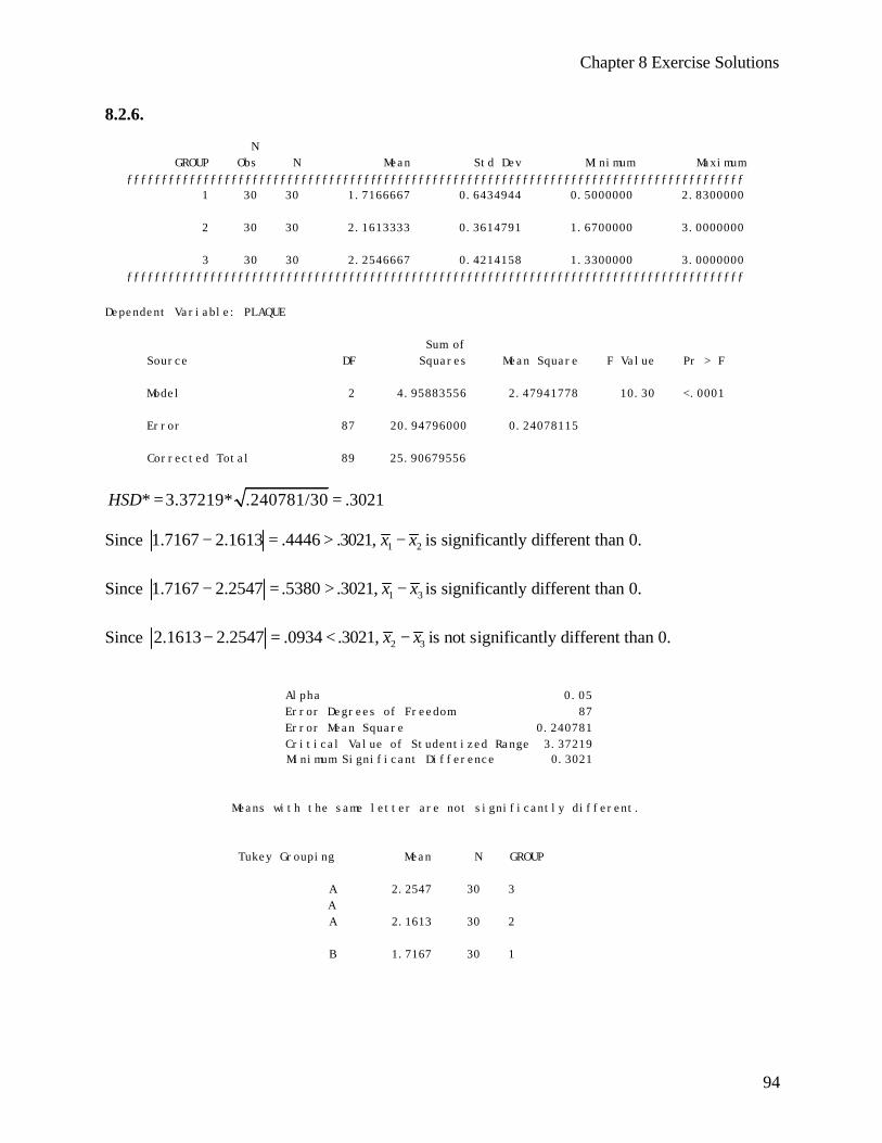
Chapter 8 Exercise Solutions
94
8.2.6. N GROUP Obs N Mean Std Dev Minimum Maximum ƒƒƒƒƒƒƒƒƒƒƒƒƒƒƒƒƒƒƒƒƒƒƒƒƒƒƒƒƒƒƒƒƒƒƒƒƒƒƒƒƒƒƒƒƒƒƒƒƒƒƒƒƒƒƒƒƒƒƒƒƒƒƒƒƒƒƒƒƒƒƒƒƒƒƒƒƒƒƒƒƒƒƒƒƒƒƒƒƒ 1 30 30 1.7166667 0.6434944 0.5000000 2.8300000 2 30 30 2.1613333 0.3614791 1.6700000 3.0000000 3 30 30 2.2546667 0.4214158 1.3300000 3.0000000 ƒƒƒƒƒƒƒƒƒƒƒƒƒƒƒƒƒƒƒƒƒƒƒƒƒƒƒƒƒƒƒƒƒƒƒƒƒƒƒƒƒƒƒƒƒƒƒƒƒƒƒƒƒƒƒƒƒƒƒƒƒƒƒƒƒƒƒƒƒƒƒƒƒƒƒƒƒƒƒƒƒƒƒƒƒƒƒƒƒ Dependent Variable: PLAQUE Sum of Source DF Squares Mean Square F Value Pr > F Model 2 4.95883556 2.47941778 10.30 <.0001 Error 87 20.94796000 0.24078115 Corrected Total 89 25.90679556
* 3.37219* .240781/30 .3021HSD = =
Since 1 21.7167 2.1613 .4446 .3021, x x− = > − is significantly different than 0. Since 1 31.7167 2.2547 .5380 .3021, x x− = > − is significantly different than 0. Since 2 32.1613 2.2547 .0934 .3021, x x− = < − is not significantly different than 0. Alpha 0.05 Error Degrees of Freedom 87 Error Mean Square 0.240781 Critical Value of Studentized Range 3.37219 Minimum Significant Difference 0.3021 Means with the same letter are not significantly different. Tukey Grouping Mean N GROUP A 2.2547 30 3 A A 2.1613 30 2 B 1.7167 30 1
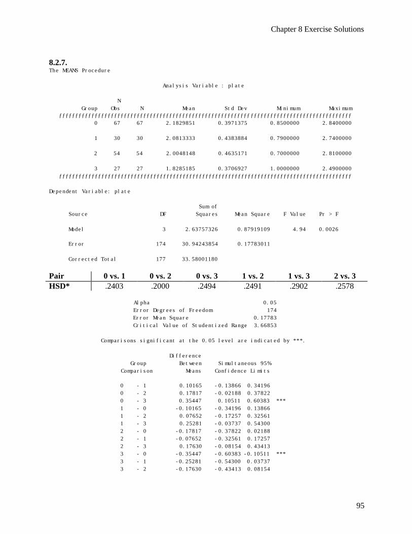
Chapter 8 Exercise Solutions
95
8.2.7. The MEANS Procedure Analysis Variable : plate N Group Obs N Mean Std Dev Minimum Maximum ƒƒƒƒƒƒƒƒƒƒƒƒƒƒƒƒƒƒƒƒƒƒƒƒƒƒƒƒƒƒƒƒƒƒƒƒƒƒƒƒƒƒƒƒƒƒƒƒƒƒƒƒƒƒƒƒƒƒƒƒƒƒƒƒƒƒƒƒƒƒƒƒƒƒƒƒƒƒƒƒƒƒƒƒƒƒƒƒƒƒ 0 67 67 2.1829851 0.3971375 0.8500000 2.8400000 1 30 30 2.0813333 0.4383884 0.7900000 2.7400000 2 54 54 2.0048148 0.4635171 0.7000000 2.8100000 3 27 27 1.8285185 0.3706927 1.0000000 2.4900000 ƒƒƒƒƒƒƒƒƒƒƒƒƒƒƒƒƒƒƒƒƒƒƒƒƒƒƒƒƒƒƒƒƒƒƒƒƒƒƒƒƒƒƒƒƒƒƒƒƒƒƒƒƒƒƒƒƒƒƒƒƒƒƒƒƒƒƒƒƒƒƒƒƒƒƒƒƒƒƒƒƒƒƒƒƒƒƒƒƒƒ Dependent Variable: plate Sum of Source DF Squares Mean Square F Value Pr > F Model 3 2.63757326 0.87919109 4.94 0.0026 Error 174 30.94243854 0.17783011 Corrected Total 177 33.58001180
Pair 0 vs. 1 0 vs. 2 0 vs. 3 1 vs. 2 1 vs. 3 2 vs. 3 HSD* .2403 .2000 .2494 .2491 .2902 .2578 Alpha 0.05 Error Degrees of Freedom 174 Error Mean Square 0.17783 Critical Value of Studentized Range 3.66853 Comparisons significant at the 0.05 level are indicated by ***. Difference Group Between Simultaneous 95% Comparison Means Confidence Limits 0 - 1 0.10165 -0.13866 0.34196 0 - 2 0.17817 -0.02188 0.37822 0 - 3 0.35447 0.10511 0.60383 *** 1 - 0 -0.10165 -0.34196 0.13866 1 - 2 0.07652 -0.17257 0.32561 1 - 3 0.25281 -0.03737 0.54300 2 - 0 -0.17817 -0.37822 0.02188 2 - 1 -0.07652 -0.32561 0.17257 2 - 3 0.17630 -0.08154 0.43413 3 - 0 -0.35447 -0.60383 -0.10511 *** 3 - 1 -0.25281 -0.54300 0.03737 3 - 2 -0.17630 -0.43413 0.08154
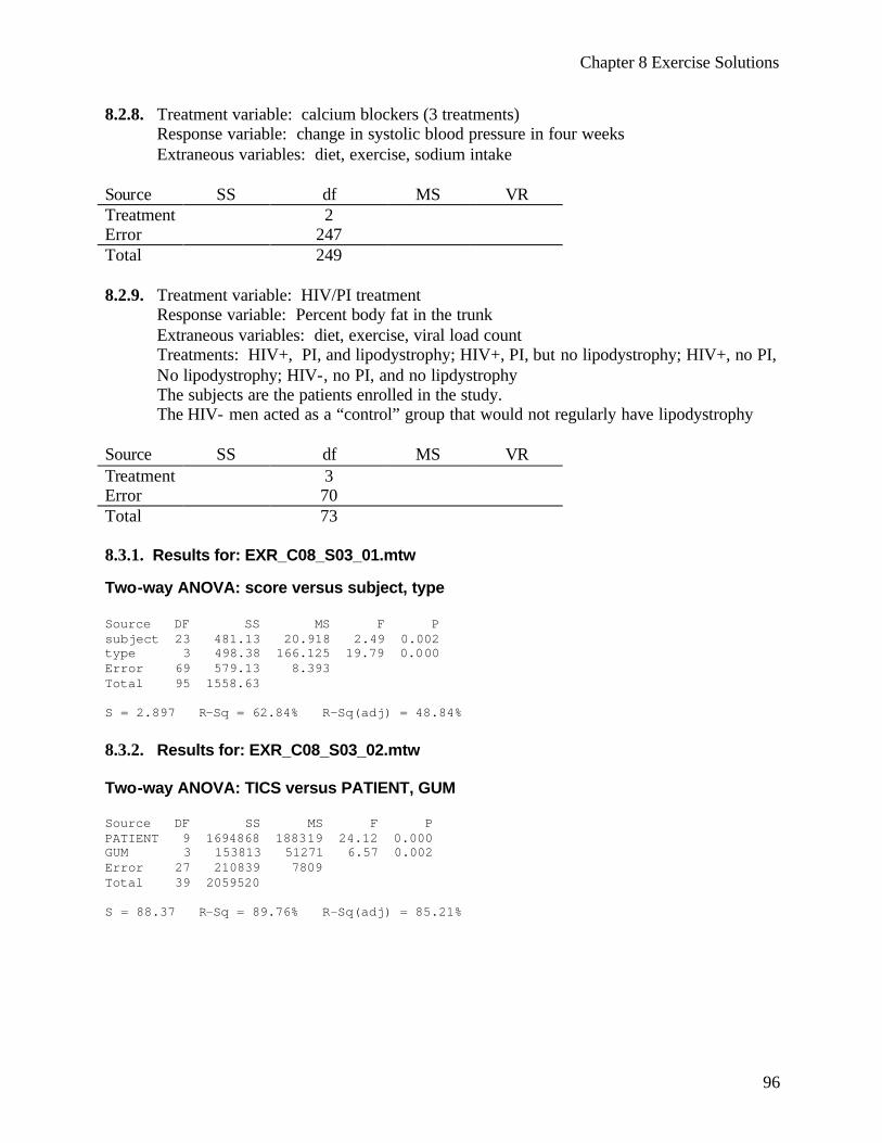
Chapter 8 Exercise Solutions
96
8.2.8. Treatment variable: calcium blockers (3 treatments) Response variable: change in systolic blood pressure in four weeks Extraneous variables: diet, exercise, sodium intake
Source SS df MS VR Treatment 2 Error 247 Total 249
8.2.9. Treatment variable: HIV/PI treatment
Response variable: Percent body fat in the trunk Extraneous variables: diet, exercise, viral load count Treatments: HIV+, PI, and lipodystrophy; HIV+, PI, but no lipodystrophy; HIV+, no PI, No lipodystrophy; HIV-, no PI, and no lipdystrophy The subjects are the patients enrolled in the study. The HIV- men acted as a “control” group that would not regularly have lipodystrophy
Source SS df MS VR Treatment 3 Error 70 Total 73 8.3.1. Results for: EXR_C08_S03_01.mtw Two-way ANOVA: score versus subject, type Source DF SS MS F P subject 23 481.13 20.918 2.49 0.002 type 3 498.38 166.125 19.79 0.000 Error 69 579.13 8.393 Total 95 1558.63 S = 2.897 R-Sq = 62.84% R-Sq(adj) = 48.84% 8.3.2. Results for: EXR_C08_S03_02.mtw Two-way ANOVA: TICS versus PATIENT, GUM Source DF SS MS F P PATIENT 9 1694868 188319 24.12 0.000 GUM 3 153813 51271 6.57 0.002 Error 27 210839 7809 Total 39 2059520 S = 88.37 R-Sq = 89.76% R-Sq(adj) = 85.21%

Chapter 8 Exercise Solutions
97
8.3.3. Results for: EXR_C08_S03_03.mtw Two-way ANOVA: SCORE versus METHOD, MOTIV Source DF SS MS F P METHOD 4 632.8 158.200 30.23 0.000 MOTIV 3 471.2 157.067 30.01 0.000 Error 12 62.8 5.233 Total 19 1166.8 S = 2.288 R-Sq = 94.62% R-Sq(adj) = 91.48% 8.3.4. Results for: EXR_C08_S03_04.mtw Two-way ANOVA: LENGTH versus NURSE, TOD Source DF SS MS F P NURSE 3 531.188 177.063 49.70 0.000 TOD 3 124.688 41.563 11.67 0.002 Error 9 32.063 3.563 Total 15 687.938 S = 1.887 R-Sq = 95.34% R-Sq(adj) = 92.23% 8.3.5. Results for: EXR_C08_S03_05.mtw Two-way ANOVA: STRESS versus SUBJ, TREAT Source DF SS MS F P SUBJ 3 260.667 86.8889 14.15 0.004 TREAT 2 90.500 45.2500 7.37 0.024 Error 6 36.833 6.1389 Total 11 388.000 S = 2.478 R-Sq = 90.51% R-Sq(adj) = 82.60% 8.3.6. Source df Blocks 7 Treatments 5 Error 35 Total 47 8.3.7. Source df Blocks 5 Treatments 56 Error 30 Total 41
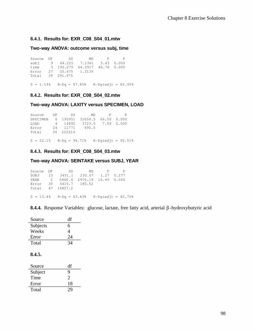
Chapter 8 Exercise Solutions
98
8.4.1. Results for: EXR_C08_S04_01.mtw Two-way ANOVA: outcome versus subj, time Source DF SS MS F P subj 9 64.225 7.1361 5.43 0.000 time 3 192.275 64.0917 48.78 0.000 Error 27 35.475 1.3139 Total 39 291.975 S = 1.146 R-Sq = 87.85% R-Sq(adj) = 82.45% 8.4.2. Results for: EXR_C08_S04_02.mtw Two-way ANOVA: LAXITY versus SPECIMEN, LOAD Source DF SS MS F P SPECIMEN 6 195951 32658.5 66.59 0.000 LOAD 4 14892 3723.0 7.59 0.000 Error 24 11771 490.5 Total 34 222614 S = 22.15 R-Sq = 94.71% R-Sq(adj) = 92.51% 8.4.3. Results for: EXR_C08_S04_03.mtw Two-way ANOVA: SEINTAKE versus SUBJ, YEAR Source DF SS MS F P SUBJ 15 3451.1 230.07 1.27 0.277 YEAR 2 5940.4 2970.19 16.45 0.000 Error 30 5415.7 180.52 Total 47 14807.2 S = 13.44 R-Sq = 63.43% R-Sq(adj) = 42.70% 8.4.4. Response Variables: glucose, lactate, free fatty acid, arterial β-hydroxybutyric acid Source df Subjects 6 Weeks 4 Error 24 Total 34 8.4.5. Source df Subject 9 Time 2 Error 18 Total 29

Chapter 8 Exercise Solutions
99
8.5.1. Results for: EXR_C08_S05_01.mtw Two-way ANOVA: Percent versus Treat, Dose Source DF SS MS F P Treat 1 2021.8 2021.8 6.18 0.023 Dose 2 48765.6 24382.8 74.59 0.000 Interaction 2 583.7 291.9 0.89 0.427 Error 18 5884.1 326.9 Total 23 57255.2 S = 18.08 R-Sq = 89.72% R-Sq(adj) = 86.87% Two-way ANOVA: Percent versus Treat, Dose Source DF SS MS F P Treat 1 2021.8 2021.8 6.25 0.021 Dose 2 48765.6 24382.8 75.40 0.000 Error 20 6467.9 323.4 Total 23 57255.2 S = 17.98 R-Sq = 88.70% R-Sq(adj) = 87.01% Since the p value for the interaction term is greater than .05, we fail to reject the null hypothesis that there is interaction. After refitting the model without the interaction, we see both dose and treatment are significant. 8.5.2. Results for: EXR_C08_S05_02.mtw Two-way ANOVA: MONTHS versus PHYS, PSYCH Source DF SS MS F P PHYS 5 13.796 2.7592 7.59 0.000 PSYCH 3 90.408 30.1359 82.91 0.000 Interaction 15 32.001 2.1334 5.87 0.000 Error 48 17.447 0.3635 Total 71 153.651 S = 0.6029 R-Sq = 88.65% R-Sq(adj) = 83.20% Since the p values are significant for physical therapy treatment, psychological treatment, and interaction, we reject the null hypothesis for each of those variables.

Chapter 8 Exercise Solutions
100
8.5.3. Results for: EXR_C08_S05_03.mtw General Linear Model: CHANGE versus MIGRAINE, TREAT Factor Type Levels Values MIGRAINE fixed 2 1, 2 TREAT fixed 2 1, 2 Analysis of Variance for CHANGE, using Adjusted SS for Tests Source DF Seq SS Adj SS Adj MS F P MIGRAINE 1 6827.3 7983.7 7983.7 19.98 0.000 TREAT 1 646.9 851.1 851.1 2.13 0.152 MIGRAINE*TREAT 1 567.3 567.3 567.3 1.42 0.240 Error 40 15979.7 15979.7 399.5 Total 43 24021.2 S = 19.9873 R-Sq = 33.48% R-Sq(adj) = 28.49% General Linear Model: CHANGE versus MIGRAINE, TREAT Factor Type Levels Values MIGRAINE fixed 2 1, 2 TREAT fixed 2 1, 2 Analysis of Variance for CHANGE, using Adjusted SS for Tests Source DF Seq SS Adj SS Adj MS F P MIGRAINE 1 6827.3 7453.1 7453.1 18.47 0.000 TREAT 1 646.9 646.9 646.9 1.60 0.213 Error 41 16546.9 16546.9 403.6 Total 43 24021.2 S = 20.0894 R-Sq = 31.12% R-Sq(adj) = 27.75% Since the p value for the interaction term is greater than .05, we fail to reject the null hypothesis that there is interaction. After refitting the model without the interaction, we see treatment remains not significant.
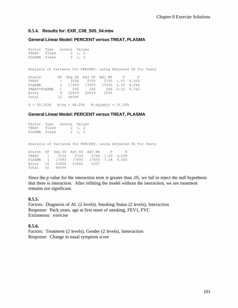
Chapter 8 Exercise Solutions
101
8.5.4. Results for: EXR_C08_S05_04.mtw General Linear Model: PERCENT versus TREAT, PLASMA Factor Type Levels Values TREAT fixed 2 1, 2 PLASMA fixed 2 1, 2 Analysis of Variance for PERCENT, using Adjusted SS for Tests Source DF Seq SS Adj SS Adj MS F P TREAT 1 3536 2705 2705 1.07 0.329 PLASMA 1 17493 13555 13555 5.35 0.046 TREAT*PLASMA 1 246 246 246 0.10 0.762 Error 9 22819 22819 2535 Total 12 44094 S = 50.3536 R-Sq = 48.25% R-Sq(adj) = 31.00% General Linear Model: PERCENT versus TREAT, PLASMA Factor Type Levels Values TREAT fixed 2 1, 2 PLASMA fixed 2 1, 2 Analysis of Variance for PERCENT, using Adjusted SS for Tests Source DF Seq SS Adj SS Adj MS F P TREAT 1 3536 2765 2765 1.20 0.299 PLASMA 1 17493 17493 17493 7.58 0.020 Error 10 23066 23066 2307 Total 12 44094 Since the p value for the interaction term is greater than .05, we fail to reject the null hypothesis that there is interaction. After refitting the model without the interaction, we see treatment remains not significant. 8.5.5. Factors: Diagnosis of AL (2 levels), Smoking Status (2 levels), Interaction Response: Pack years, age at first onset of smoking, FEV1, FVC Extraneous: exercise 8.5.6. Factors: Treatment (2 levels), Gender (2 levels), Ineteraction Response: Change in nasal symptom score
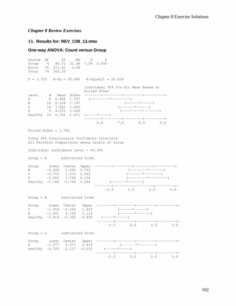
Chapter 8 Exercise Solutions
102
Chapter 8 Review Exercises 13. Results for: REV_C08_13.mtw One-way ANOVA: Count versus Group Source DF SS MS F P Group 4 86.72 21.68 7.04 0.000 Error 70 215.62 3.08 Total 74 302.35 S = 1.755 R-Sq = 28.68% R-Sq(adj) = 24.61% Individual 95% CIs For Mean Based on Pooled StDev Level N Mean StDev --------+---------+---------+---------+- A 8 6.488 1.767 (---------*---------) B 18 8.128 1.797 (------*------) C 16 7.862 1.640 (-------*------) D 9 8.233 2.469 (---------*--------) healthy 24 5.746 1.471 (-----*-----) --------+---------+---------+---------+- 6.0 7.2 8.4 9.6 Pooled StDev = 1.755 Tukey 95% Simultaneous Confidence Intervals All Pairwise Comparisons among Levels of Group Individual confidence level = 99.34% Group = A subtracted from: Group Lower Center Upper --------+---------+---------+---------+- B -0.448 1.640 3.729 (--------*-------) C -0.753 1.375 3.503 (-------*--------) D -0.642 1.746 4.134 (---------*---------) healthy -2.748 -0.742 1.265 (-------*-------) --------+---------+---------+---------+- -2.5 0.0 2.5 5.0 Group = B subtracted from: Group Lower Center Upper --------+---------+---------+---------+- C -1.954 -0.265 1.423 (------*------) D -1.901 0.106 2.112 (-------*-------) healthy -3.914 -2.382 -0.850 (-----*------) --------+---------+---------+---------+- -2.5 0.0 2.5 5.0 Group = C subtracted from: Group Lower Center Upper --------+---------+---------+---------+- D -1.677 0.371 2.419 (-------*--------) healthy -3.703 -2.117 -0.531 (------*-----) --------+---------+---------+---------+- -2.5 0.0 2.5 5.0
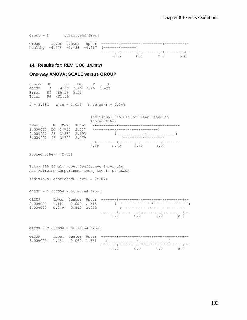
Chapter 8 Exercise Solutions
103
Group = D subtracted from: Group Lower Center Upper --------+---------+---------+---------+- healthy -4.408 -2.488 -0.567 (-------*-------) --------+---------+---------+---------+- -2.5 0.0 2.5 5.0 14. Results for: REV_CO8_14.mtw One-way ANOVA: SCALE versus GROUP Source DF SS MS F P GROUP 2 4.98 2.49 0.45 0.639 Error 88 486.59 5.53 Total 90 491.56 S = 2.351 R-Sq = 1.01% R-Sq(adj) = 0.00% Individual 95% CIs For Mean Based on Pooled StDev Level N Mean StDev -+---------+---------+---------+-------- 1.000000 20 3.085 2.337 (--------------*--------------) 2.000000 23 3.687 2.693 (-------------*-------------) 3.000000 48 3.627 2.179 (---------*--------) -+---------+---------+---------+-------- 2.10 2.80 3.50 4.20 Pooled StDev = 2.351 Tukey 95% Simultaneous Confidence Intervals All Pairwise Comparisons among Levels of GROUP Individual confidence level = 98.07% GROUP = 1.000000 subtracted from: GROUP Lower Center Upper -------+---------+---------+---------+-- 2.000000 -1.111 0.602 2.315 (----------------*----------------) 3.000000 -0.949 0.542 2.033 (-------------*--------------) -------+---------+---------+---------+-- -1.0 0.0 1.0 2.0 GROUP = 2.000000 subtracted from: GROUP Lower Center Upper -------+---------+---------+---------+-- 3.000000 -1.481 -0.060 1.361 (-------------*--------------) -------+---------+---------+---------+-- -1.0 0.0 1.0 2.0
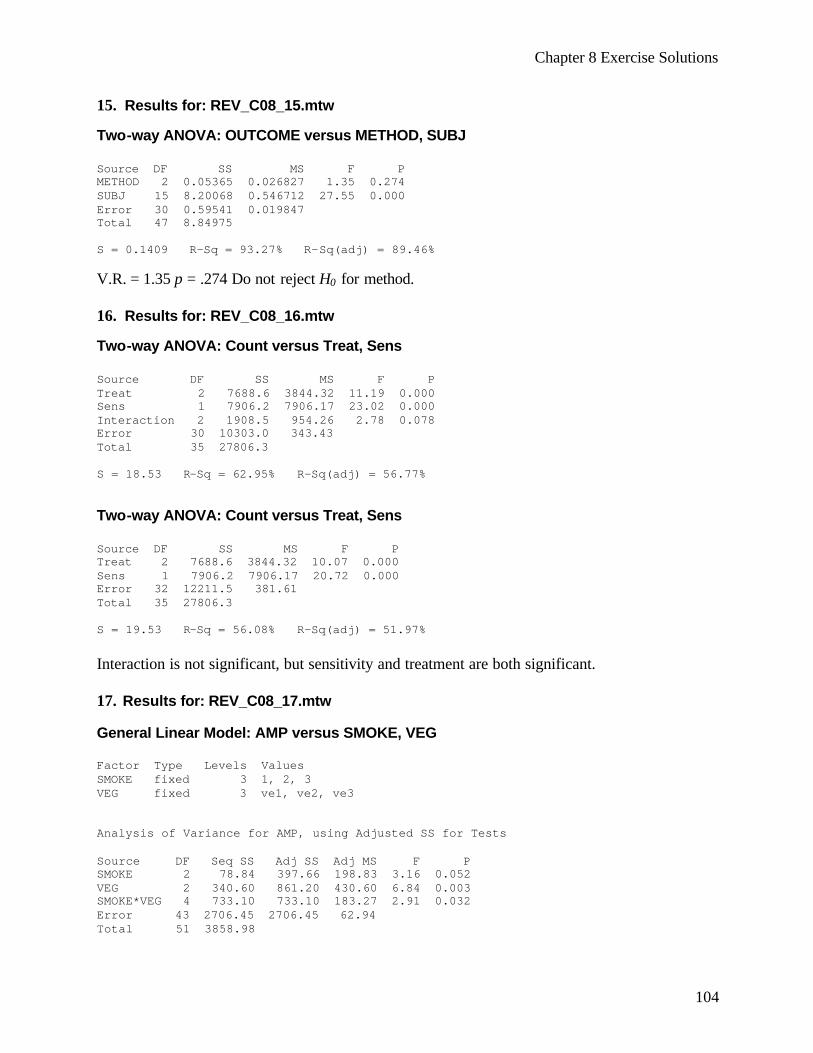
Chapter 8 Exercise Solutions
104
15. Results for: REV_C08_15.mtw Two-way ANOVA: OUTCOME versus METHOD, SUBJ Source DF SS MS F P METHOD 2 0.05365 0.026827 1.35 0.274 SUBJ 15 8.20068 0.546712 27.55 0.000 Error 30 0.59541 0.019847 Total 47 8.84975 S = 0.1409 R-Sq = 93.27% R-Sq(adj) = 89.46% V.R. = 1.35 p = .274 Do not reject H0 for method. 16. Results for: REV_C08_16.mtw Two-way ANOVA: Count versus Treat, Sens Source DF SS MS F P Treat 2 7688.6 3844.32 11.19 0.000 Sens 1 7906.2 7906.17 23.02 0.000 Interaction 2 1908.5 954.26 2.78 0.078 Error 30 10303.0 343.43 Total 35 27806.3 S = 18.53 R-Sq = 62.95% R-Sq(adj) = 56.77% Two-way ANOVA: Count versus Treat, Sens Source DF SS MS F P Treat 2 7688.6 3844.32 10.07 0.000 Sens 1 7906.2 7906.17 20.72 0.000 Error 32 12211.5 381.61 Total 35 27806.3 S = 19.53 R-Sq = 56.08% R-Sq(adj) = 51.97% Interaction is not significant, but sensitivity and treatment are both significant. 17. Results for: REV_C08_17.mtw General Linear Model: AMP versus SMOKE, VEG Factor Type Levels Values SMOKE fixed 3 1, 2, 3 VEG fixed 3 ve1, ve2, ve3 Analysis of Variance for AMP, using Adjusted SS for Tests Source DF Seq SS Adj SS Adj MS F P SMOKE 2 78.84 397.66 198.83 3.16 0.052 VEG 2 340.60 861.20 430.60 6.84 0.003 SMOKE*VEG 4 733.10 733.10 183.27 2.91 0.032 Error 43 2706.45 2706.45 62.94 Total 51 3858.98

Chapter 8 Exercise Solutions
105
18. Results for: REV_C08_18.mtw One-way ANOVA: length versus site Source DF SS MS F P site 2 0.768 0.384 1.97 0.148 Error 71 13.865 0.195 Total 73 14.633 S = 0.4419 R-Sq = 5.25% R-Sq(adj) = 2.58% One-way ANOVA: width versus site Source DF SS MS F P site 2 0.519 0.259 1.36 0.262 Error 71 13.502 0.190 Total 73 14.021 S = 0.4361 R-Sq = 3.70% R-Sq(adj) = 0.99% One-way ANOVA: height versus site Source DF SS MS F P site 2 0.609 0.304 1.72 0.187 Error 71 12.594 0.177 Total 73 13.203 S = 0.4212 R-Sq = 4.61% R-Sq(adj) = 1.92% Fail to reject the null hypothesis for a difference in length, width, or height at the different locations. 19. Results for: REV_C08_19.mtw Two-way ANOVA: EMG versus SUBJ, ANGLE Source DF SS MS F P SUBJ 17 14405.2 847.365 12.05 0.000 ANGLE 8 2376.2 297.020 4.23 0.000 Error 136 9560.2 70.296 Total 161 26341.6 S = 8.384 R-Sq = 63.71% R-Sq(adj) = 57.04%
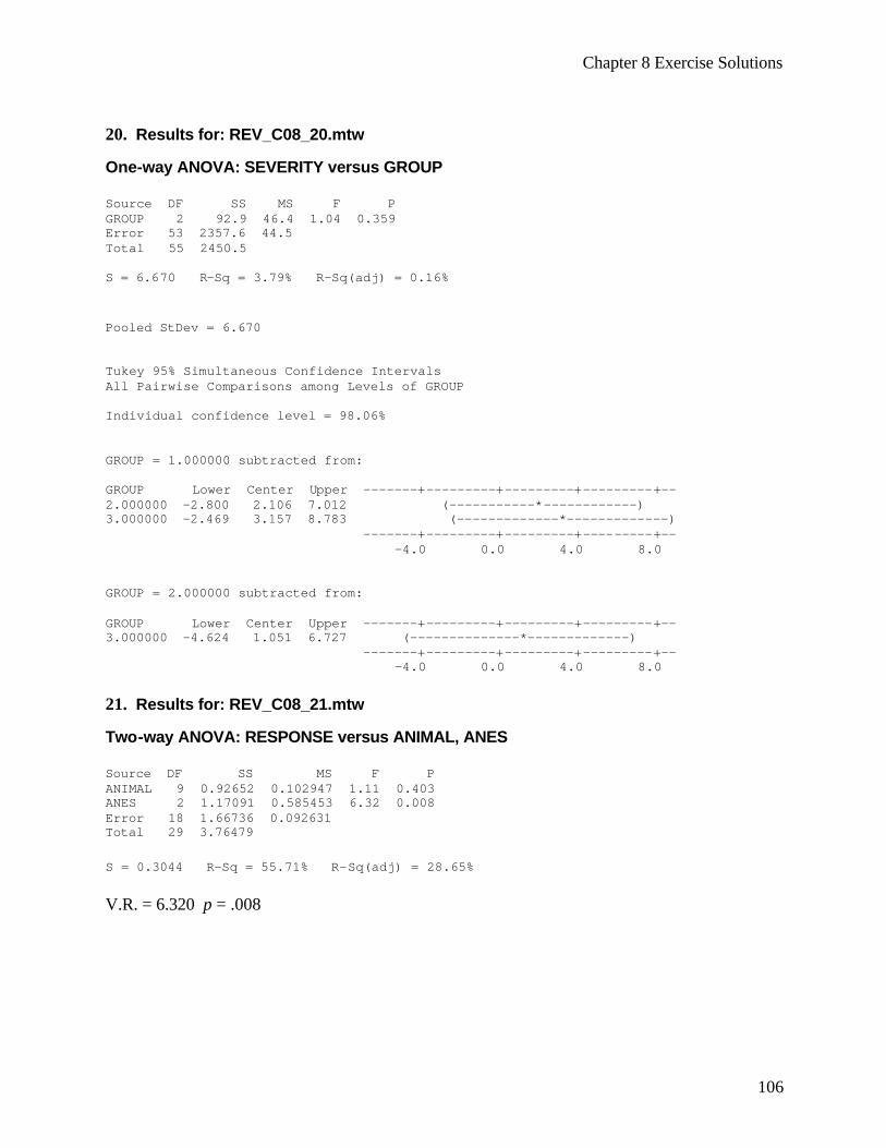
Chapter 8 Exercise Solutions
106
20. Results for: REV_C08_20.mtw One-way ANOVA: SEVERITY versus GROUP Source DF SS MS F P GROUP 2 92.9 46.4 1.04 0.359 Error 53 2357.6 44.5 Total 55 2450.5 S = 6.670 R-Sq = 3.79% R-Sq(adj) = 0.16% Pooled StDev = 6.670 Tukey 95% Simultaneous Confidence Intervals All Pairwise Comparisons among Levels of GROUP Individual confidence level = 98.06% GROUP = 1.000000 subtracted from: GROUP Lower Center Upper -------+---------+---------+---------+-- 2.000000 -2.800 2.106 7.012 (-----------*------------) 3.000000 -2.469 3.157 8.783 (-------------*-------------) -------+---------+---------+---------+-- -4.0 0.0 4.0 8.0 GROUP = 2.000000 subtracted from: GROUP Lower Center Upper -------+---------+---------+---------+-- 3.000000 -4.624 1.051 6.727 (--------------*-------------) -------+---------+---------+---------+-- -4.0 0.0 4.0 8.0 21. Results for: REV_C08_21.mtw Two-way ANOVA: RESPONSE versus ANIMAL, ANES Source DF SS MS F P ANIMAL 9 0.92652 0.102947 1.11 0.403 ANES 2 1.17091 0.585453 6.32 0.008 Error 18 1.66736 0.092631 Total 29 3.76479 S = 0.3044 R-Sq = 55.71% R-Sq(adj) = 28.65% V.R. = 6.320 p = .008

Chapter 8 Exercise Solutions
107
22. Results for: REV_C08_22.mtw General Linear Model: SCORES versus SIDE, SIZE Factor Type Levels Values SIDE fixed 2 L, R SIZE fixed 3 2, 3, 4 Analysis of Variance for SCORES, using Adjusted SS for Tests Source DF Seq SS Adj SS Adj MS F P SIDE 1 1.287 2.662 2.662 0.66 0.421 SIZE 2 29.981 37.651 18.826 4.66 0.014 SIDE*SIZE 2 10.540 10.540 5.270 1.31 0.281 Error 48 193.840 193.840 4.038 Total 53 235.648 S = 2.00956 R-Sq = 17.74% R-Sq(adj) = 9.17% Analysis of Variance for SCORES, using Adjusted SS for Tests Source DF Seq SS Adj SS Adj MS F P SIDE 1 1.287 2.578 2.578 0.63 0.431 SIZE 2 29.981 29.981 14.991 3.67 0.033 Error 50 204.380 204.380 4.088 Total 53 235.648 S = 2.02178 R-Sq = 13.27% R-Sq(adj) = 8.07% Interaction is not significant, nor is side of the brain. 23. Results for: REV_C08_23.mtw One-way ANOVA: WEIGHT versus GROUP Source DF SS MS F P GROUP 3 1037901 345967 3.12 0.043 Error 27 2995421 110942 Total 30 4033323 GROUP = A subtracted from: GROUP Lower Center Upper ---------+---------+---------+---------+ B -169.3 302.4 774.1 (--------*--------) C -657.2 -164.9 327.3 (---------*---------) D -587.4 -155.1 277.3 (--------*--------) ---------+---------+---------+---------+ -500 0 500 1000
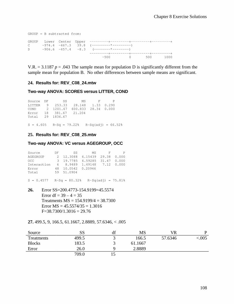
Chapter 8 Exercise Solutions
108
GROUP = B subtracted from: GROUP Lower Center Upper ---------+---------+---------+---------+ C -974.4 -467.3 39.8 (---------*---------) D -906.6 -457.4 -8.3 (--------*--------) ---------+---------+---------+---------+ -500 0 500 1000 V.R. = 3.1187 p = .043 The sample mean for population D is significantly different from the sample mean for population B. No other differences between sample means are significant. 24. Results for: REV_C08_24.mtw Two-way ANOVA: SCORES versus LITTER, COND Source DF SS MS F P LITTER 9 253.33 28.148 1.33 0.290 COND 2 1201.67 600.833 28.34 0.000 Error 18 381.67 21.204 Total 29 1836.67 S = 4.605 R-Sq = 79.22% R-Sq(adj) = 66.52% 25. Results for: REV_C08_25.mtw Two-way ANOVA: VC versus AGEGROUP, OCC Source DF SS MS F P AGEGROUP 2 12.3088 6.15439 29.38 0.000 OCC 3 19.7785 6.59285 31.47 0.000 Interaction 6 8.9489 1.49148 7.12 0.000 Error 48 10.0542 0.20946 Total 59 51.0904 S = 0.4577 R-Sq = 80.32% R-Sq(adj) = 75.81% 26. Error SS=200.4773-154.9199=45.5574 Error df = 39 – 4 = 35 Treatments MS = 154.9199/4 = 38.7300 Error MS = 45.5574/35 = 1.3016 F=38.7300/1.3016 = 29.76 27. 499.5, 9, 166.5, 61.1667, 2.8889, 57.6346, < .005 Source SS df MS VR P Treatments 499.5 3 166.5 57.6346 <.005 Blocks 183.5 3 61.1667 Error 26.0 9 2.8889 709.0 15

Chapter 8 Exercise Solutions
109
28. (a) Analysis for a factorial experiment (b) There is a significant difference among levels of factor A, and among levels of factor B,
and there is also a significant interaction effect, since all three p values are < .005. 29. (a) Completely randomized (b) 3 (c) 30 (d) No, because 1.0438 < 3.35 30. (a) Randomized complete block design
(b) 3 (c) 24 (d) No, because 2.824 < 3.74 31. Dependent Variable: SERUM Sum of Source DF Squares Mean Square F Value Pr > F Model 3 216.8571429 72.2857143 26.06 <.0001 Error 24 66.5714286 2.7738095 Corrected Total 27 283.4285714 R-Square Coeff Var Root MSE SERUM Mean 0.765121 23.31666 1.665476 7.142857 Pooled St. Dev. = Root MSE = 1.665 HSD = 3.90126 2.7738095/7 2.4458= Alpha 0.05 Error Degrees of Freedom 24 Error Mean Square 2.77381 Critical Value of Studentized Range 3.90126 Minimum Significant Difference 2.4558
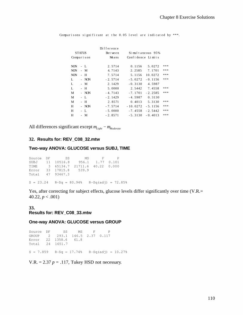
Chapter 8 Exercise Solutions
110
Comparisons significant at the 0.05 level are indicated by ***. Difference STATUS Between Simultaneous 95% Comparison Means Confidence Limits NON - L 2.5714 0.1156 5.0272 *** NON - M 4.7143 2.2585 7.1701 *** NON - H 7.5714 5.1156 10.0272 *** L - NON -2.5714 -5.0272 -0.1156 *** L - M 2.1429 -0.3130 4.5987 L - H 5.0000 2.5442 7.4558 *** M - NON -4.7143 -7.1701 -2.2585 *** M - L -2.1429 -4.5987 0.3130 M - H 2.8571 0.4013 5.3130 *** H - NON -7.5714 -10.0272 -5.1156 *** H - L -5.0000 -7.4558 -2.5442 *** H - M -2.8571 -5.3130 -0.4013 *** All differences significant except Light Moderateµ µ− 32. Results for: REV_C08_32.mtw Two-way ANOVA: GLUCOSE versus SUBJ, TIME Source DF SS MS F P SUBJ 11 10516.8 956.1 1.77 0.101 TIME 3 65134.7 21711.6 40.22 0.000 Error 33 17815.8 539.9 Total 47 93467.3 S = 23.24 R-Sq = 80.94% R-Sq(adj) = 72.85% Yes, after correcting for subject effects, glucose levels differ significantly over time (V.R.= 40.22, p < .001) 33. Results for: REV_C08_33.mtw One-way ANOVA: GLUCOSE versus GROUP Source DF SS MS F P GROUP 2 293.1 146.5 2.37 0.117 Error 22 1358.6 61.8 Total 24 1651.7 S = 7.859 R-Sq = 17.74% R-Sq(adj) = 10.27% V.R. = 2.37 p = .117, Tukey HSD not necessary.
Chapter 8 Exercise Solutions
111
34. (a) Repeated measures design
(b) Response: Reduced and Oxidized Vitamin C content (there are 2 response variables)
(c) Factors: juice packages (unknown number of levels) and Time (13 levels).
(d) Storage temperature, whether juice made from concentrate or not
(e) Carry over effects not applicable here as there is no treatment being administered
(f) Unable to do with information provided.
35. (a) One way ANOVA
(b) Response: Post-Pre training score
(c) Factors: Groups of years of experience (4 levels).
(d) Interest in obstetrics, surgical experience
(e) No carry over effects
(f) treatment is years of experience d.f.=3, total d.f. = 29, error d.f. = 26. 36.
(a) One way ANOVA
(b) Response: Vascular endothelial growth factor, leptin, TNF-α plasma protein and full blood count
(c) Factors: Pregnancy status (3 levels).
(d) Weeks along in pregnancy, stress
(e) No carry over effects
(f) Treatment is pregnancy status d.f.=2, total d.f. = 53, error d.f. = 51.
Chapter 8 Exercise Solutions
112
37. (a) Repeated measures
(b) Response: BMD
(c) Factors: Time points (6 levels)
(d) Diet, exercise, calcium intake
(e) No carry over effects
(f) time factor d.f. = 5, subject factor d.f. = 25, total d.f. = 155, error d.f.= 125.
38.
(a) 2 Way ANOVA
(b) Response: Cleavage rate and birth rate of pups
(c) Factors: Donor Cell types (2 levels) and Genotypes (6 levels)
(d) Need to know more about mouse cloning
(e) No carry over effects
(f) Donor cell type d.f. = , Genotype factor d.f. = 5, total d.f. = unknown, error d.f.= unknown.
39. Analysis of Variance for bilirubi Source DF SS MS F P subject 17 2480.83 145.93 45.57 0.000 time 6 89.09 14.85 4.64 0.000 Error 102 326.65 3.20 Total 125 2896.57 40. Results for: REV_C08_40.mtw One-way ANOVA: B-T versus Group Source DF SS MS F P Group 2 31 15 0.15 0.860 Error 27 2747 102 Total 29 2777 S = 10.09 R-Sq = 1.11% R-Sq(adj) = 0.00% Tukey procedure not warranted since p >.05
Chapter 8 Exercise Solutions
113
41. CR= Compression Ratio Analysis of Variance for C.R. Source DF SS MS F P Group 4 9092 2273 8.12 0.001 Error 19 5319 280 Total 23 14411 Individual 95% CIs For Mean Based on Pooled StDev Level N Mean StDev ---+---------+---------+---------+--- Control 6 79.96 5.46 (-----*-----) I 4 78.69 21.44 (------*------) II 4 47.84 23.74 (------*------) III 5 43.51 10.43 (-----*------) IV 5 33.32 20.40 (-----*------) ---+---------+---------+---------+--- Pooled StDev = 16.73 25 50 75 100 Tukey's pairwise comparisons Family error rate = 0.0500 Individual error rate = 0.00728 Critical value = 4.25 Intervals for (column level mean) - (row level mean) Control I II III I -31.19 33.72 II -0.34 -4.70 64.58 66.41 III 6.00 1.45 -29.41 66.89 68.91 38.05 IV 16.19 11.64 -19.21 -21.61 77.08 79.10 48.24 41.99 42. One approach is too look to see if differences exist between the 3 groups at the 7 time points. One-way ANOVA: MIN0 versus GROUP Source DF SS MS F P GROUP 2 1026 513 1.39 0.289 Error 11 4053 368 Total 13 5079 S = 19.19 R-Sq = 20.20% R-Sq(adj) = 5.70% Individual 95% CIs For Mean Based on Pooled StDev Level N Mean StDev ----+---------+---------+---------+----- C 5 76.80 19.08 (-----------*-----------) F 5 80.40 22.32 (-----------*-----------) P 4 97.25 14.17 (------------*------------) ----+---------+---------+---------+----- 64 80 96 112 Pooled StDev = 19.19
Chapter 8 Exercise Solutions
114
One-way ANOVA: MIN60 versus GROUP Source DF SS MS F P GROUP 2 704 352 1.44 0.278 Error 11 2686 244 Total 13 3390 S = 15.63 R-Sq = 20.77% R-Sq(adj) = 6.37% Individual 95% CIs For Mean Based on Pooled StDev Level N Mean StDev ------+---------+---------+---------+--- C 5 77.80 15.48 (---------*---------) F 5 85.80 20.38 (---------*---------) P 4 68.00 4.69 (----------*-----------) ------+---------+---------+---------+--- 60 75 90 105 Pooled StDev = 15.63 One-way ANOVA: MIN120 versus GROUP Source DF SS MS F P GROUP 2 2435 1217 2.21 0.156 Error 11 6065 551 Total 13 8500 S = 23.48 R-Sq = 28.64% R-Sq(adj) = 15.67% Individual 95% CIs For Mean Based on Pooled StDev Level N Mean StDev -------+---------+---------+---------+-- C 5 78.80 27.07 (----------*-----------) F 5 102.40 24.11 (----------*-----------) P 4 71.50 16.42 (------------*------------) -------+---------+---------+---------+-- 60 80 100 120 Pooled StDev = 23.48 One-way ANOVA: MIN180 versus GROUP Source DF SS MS F P GROUP 2 4710 2355 4.04 0.048 Error 11 6418 583 Total 13 11128 S = 24.15 R-Sq = 42.33% R-Sq(adj) = 31.84% Individual 95% CIs For Mean Based on Pooled StDev Level N Mean StDev ---+---------+---------+---------+------ C 5 68.80 26.33 (---------*--------) F 5 107.60 21.77 (--------*---------) P 4 70.00 24.15 (----------*----------) ---+---------+---------+---------+------ 50 75 100 125 Pooled StDev = 24.15
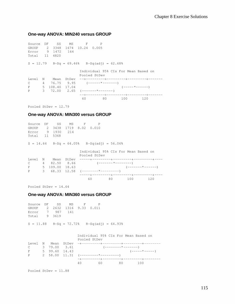
Chapter 8 Exercise Solutions
115
One-way ANOVA: MIN240 versus GROUP Source DF SS MS F P GROUP 2 3348 1674 10.24 0.005 Error 9 1472 164 Total 11 4820 S = 12.79 R-Sq = 69.46% R-Sq(adj) = 62.68% Individual 95% CIs For Mean Based on Pooled StDev Level N Mean StDev --+---------+---------+---------+------- C 4 76.75 9.95 (------*-------) F 5 108.40 17.04 (-----*------) P 3 72.00 2.65 (-------*-------) --+---------+---------+---------+------- 60 80 100 120 Pooled StDev = 12.79 One-way ANOVA: MIN300 versus GROUP Source DF SS MS F P GROUP 2 3438 1719 8.02 0.010 Error 9 1930 214 Total 11 5368 S = 14.64 R-Sq = 64.05% R-Sq(adj) = 56.06% Individual 95% CIs For Mean Based on Pooled StDev Level N Mean StDev -----+---------+---------+---------+---- C 4 82.50 8.66 (-------*--------) F 5 109.00 18.63 (-------*------) P 3 68.33 12.58 (--------*---------) -----+---------+---------+---------+---- 60 80 100 120 Pooled StDev = 14.64 One-way ANOVA: MIN360 versus GROUP Source DF SS MS F P GROUP 2 2632 1316 9.33 0.011 Error 7 987 141 Total 9 3619 S = 11.88 R-Sq = 72.72% R-Sq(adj) = 64.93% Individual 95% CIs For Mean Based on Pooled StDev Level N Mean StDev -+---------+---------+---------+-------- C 3 79.00 3.61 (--------*-------) F 5 99.60 14.43 (-----*-----) P 2 58.00 11.31 (---------*---------) -+---------+---------+---------+-------- 40 60 80 100 Pooled StDev = 11.88
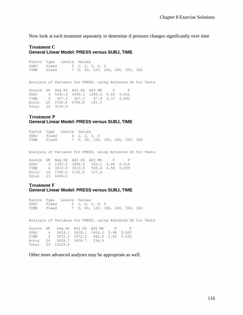
Chapter 8 Exercise Solutions
116
Now look at each treatment separately to determine if pressure changes significantly over time Treatment C General Linear Model: PRESS versus SUBJ, TIME Factor Type Levels Values SUBJ fixed 5 1, 2, 3, 4, 5 TIME fixed 7 0, 60, 120, 180, 240, 300, 360 Analysis of Variance for PRESS, using Adjusted SS for Tests Source DF Seq SS Adj SS Adj MS F P SUBJ 4 5041.8 4960.1 1240.0 6.69 0.001 TIME 6 407.3 407.3 67.9 0.37 0.892 Error 20 3706.8 3706.8 185.3 Total 30 9155.9 Treatment P General Linear Model: PRESS versus SUBJ, TIME Factor Type Levels Values SUBJ fixed 4 1, 2, 3, 4 TIME fixed 7 0, 60, 120, 180, 240, 300, 360 Analysis of Variance for PRESS, using Adjusted SS for Tests Source DF Seq SS Adj SS Adj MS F P SUBJ 3 1392.5 1896.4 632.1 4.94 0.015 TIME 6 3513.5 3513.5 585.6 4.58 0.009 Error 14 1790.0 1790.0 127.9 Total 23 6696.0 Treatment F General Linear Model: PRESS versus SUBJ, TIME Factor Type Levels Values SUBJ fixed 5 1, 2, 3, 4, 5 TIME fixed 7 0, 60, 120, 180, 240, 300, 360 Analysis of Variance for PRESS, using Adjusted SS for Tests Source DF Seq SS Adj SS Adj MS F P SUBJ 4 5618.1 5618.1 1404.5 5.98 0.002 TIME 6 3972.2 3972.2 662.0 2.82 0.032 Error 24 5638.7 5638.7 234.9 Total 34 15229.0 Other more advanced analyses may be appropriate as well.
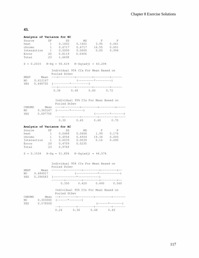
Chapter 8 Exercise Solutions
117
43. Analysis of Variance for BC Source DF SS MS F P heat 1 0.1602 0.1602 3.95 0.061 chromo 1 0.6717 0.6717 16.55 0.001 Interaction 1 0.0000 0.0000 0.00 0.994 Error 20 0.8119 0.0406 Total 23 1.6438 S = 0.2015 R-Sq = 50.61% R-Sq(adj) = 43.20% Individual 95% CIs For Mean Based on Pooled StDev HEAT Mean ---+---------+---------+---------+------ NO 0.612167 (---------*---------) YES 0.448750 (---------*----------) ---+---------+---------+---------+------ 0.36 0.48 0.60 0.72 Individual 95% CIs For Mean Based on Pooled StDev CHROMO Mean ----+---------+---------+---------+----- NO 0.363167 (-------*-------) YES 0.697750 (--------*-------) ----+---------+---------+---------+----- 0.30 0.45 0.60 0.75 Analysis of Variance for AC Source DF SS MS F P heat 1 0.0468 0.0468 1.99 0.174 chromo 1 0.4554 0.4554 19.34 0.000 Interaction 1 0.0039 0.0039 0.16 0.690 Error 20 0.4709 0.0235 Total 23 0.9769 S = 0.1534 R-Sq = 51.80% R-Sq(adj) = 44.57% Individual 95% CIs For Mean Based on Pooled StDev HEAT Mean -------+---------+---------+---------+-- NO 0.484917 (------------*------------) YES 0.396583 (-------------*------------) -------+---------+---------+---------+-- 0.350 0.420 0.490 0.560 Individual 95% CIs For Mean Based on Pooled StDev CHROMO Mean --+---------+---------+---------+------- NO 0.303000 (------*-------) YES 0.578500 (------*-------) --+---------+---------+---------+------- 0.24 0.36 0.48 0.60
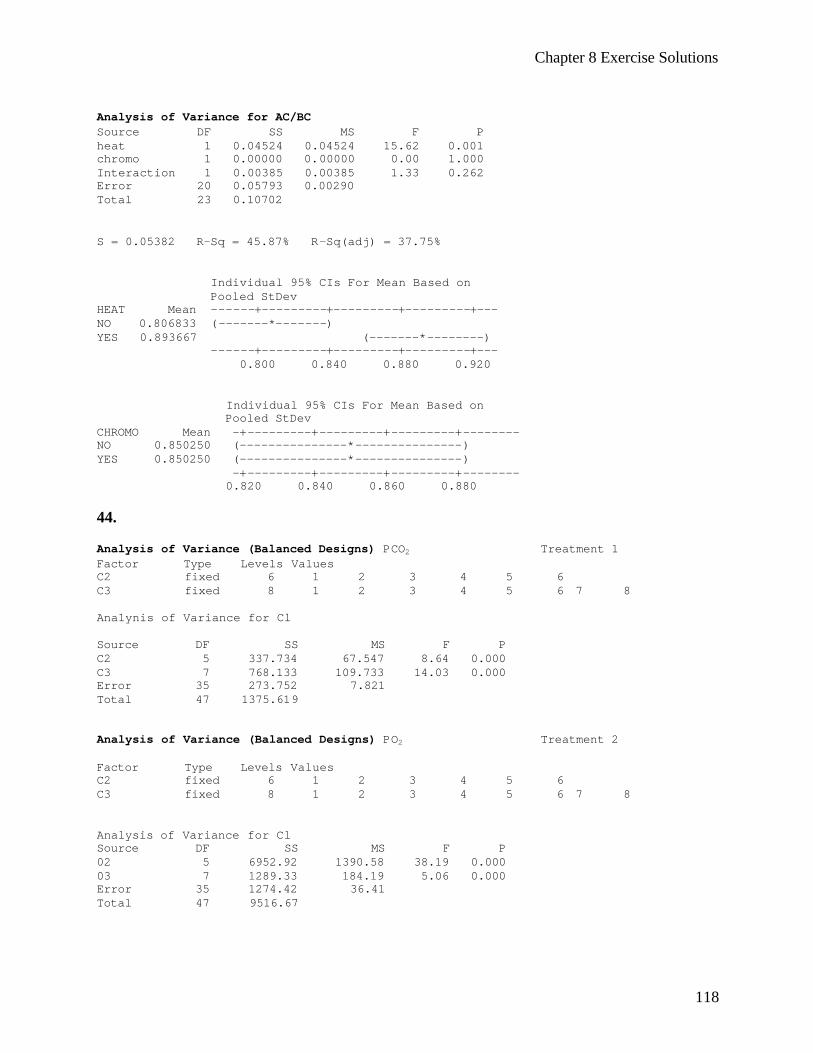
Chapter 8 Exercise Solutions
118
Analysis of Variance for AC/BC Source DF SS MS F P heat 1 0.04524 0.04524 15.62 0.001 chromo 1 0.00000 0.00000 0.00 1.000 Interaction 1 0.00385 0.00385 1.33 0.262 Error 20 0.05793 0.00290 Total 23 0.10702 S = 0.05382 R-Sq = 45.87% R-Sq(adj) = 37.75% Individual 95% CIs For Mean Based on Pooled StDev HEAT Mean ------+---------+---------+---------+--- NO 0.806833 (-------*-------) YES 0.893667 (-------*--------) ------+---------+---------+---------+--- 0.800 0.840 0.880 0.920 Individual 95% CIs For Mean Based on Pooled StDev CHROMO Mean -+---------+---------+---------+-------- NO 0.850250 (---------------*---------------) YES 0.850250 (---------------*---------------) -+---------+---------+---------+-------- 0.820 0.840 0.860 0.880 44. Analysis of Variance (Balanced Designs) PCO2 Treatment 1 Factor Type Levels Values C2 fixed 6 1 2 3 4 5 6 C3 fixed 8 1 2 3 4 5 6 7 8 Ana1ynis of Variance for Cl Source DF SS MS F P C2 5 337.734 67.547 8.64 0.000 C3 7 768.133 109.733 14.03 0.000 Error 35 273.752 7.821 Total 47 1375.619 Analysis of Variance (Balanced Designs) PO2 Treatment 2 Factor Type Levels Values C2 fixed 6 1 2 3 4 5 6 C3 fixed 8 1 2 3 4 5 6 7 8 Analysis of Variance for Cl Source DF SS MS F P 02 5 6952.92 1390.58 38.19 0.000 03 7 1289.33 184.19 5.06 0.000 Error 35 1274.42 36.41 Total 47 9516.67
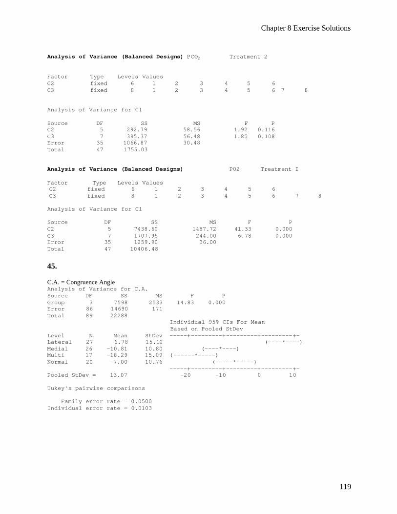
Chapter 8 Exercise Solutions
119
Analysis of Variance (Balanced Designs) PCO2 Treatment 2 Factor Type Levels Values C2 fixed 6 1 2 3 4 5 6 C3 fixed 8 1 2 3 4 5 6 7 8 Analysis of Variance for Cl Source DF SS MS F P C2 5 292.79 58.56 1.92 0.116 C3 7 395.37 56.48 1.85 0.108 Error 35 1066.87 30.48 Total 47 1755.03 Analysis of Variance (Balanced Designs) P02 Treatment I Factor Type Levels Values C2 fixed 6 1 2 3 4 5 6 C3 fixed 8 1 2 3 4 5 6 7 8 Analysis of Variance for Cl Source DF SS MS F P C2 5 7438.60 1487.72 4l.33 0.000 C3 7 1707.95 244.00 6.78 0.000 Error 35 1259.90 36.00 Total 47 10406.48 45. C.A. = Congruence Angle Analysis of Variance for C.A. Source DF SS MS F P Group 3 7598 2533 14.83 0.000 Error 86 14690 171 Total 89 22288 Individual 95% CIs For Mean Based on Pooled StDev Level N Mean StDev -----+---------+---------+---------+- Lateral 27 6.78 15.10 (----*----) Medial 26 -10.81 10.80 (----*----) Multi 17 -18.29 15.09 (------*-----) Normal 20 -7.00 10.76 (-----*-----) -----+---------+---------+---------+- Pooled StDev = 13.07 -20 -10 0 10 Tukey's pairwise comparisons Family error rate = 0.0500 Individual error rate = 0.0103
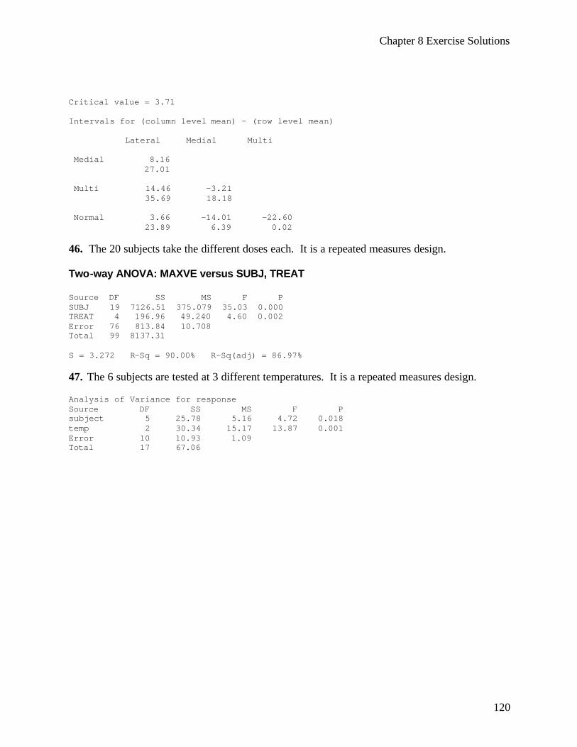
Chapter 8 Exercise Solutions
120
Critical value = 3.71 Intervals for (column level mean) - (row level mean) Lateral Medial Multi Medial 8.16 27.01 Multi 14.46 -3.21 35.69 18.18 Normal 3.66 -14.01 -22.60 23.89 6.39 0.02 46. The 20 subjects take the different doses each. It is a repeated measures design. Two-way ANOVA: MAXVE versus SUBJ, TREAT Source DF SS MS F P SUBJ 19 7126.51 375.079 35.03 0.000 TREAT 4 196.96 49.240 4.60 0.002 Error 76 813.84 10.708 Total 99 8137.31 S = 3.272 R-Sq = 90.00% R-Sq(adj) = 86.97% 47. The 6 subjects are tested at 3 different temperatures. It is a repeated measures design. Analysis of Variance for response Source DF SS MS F P subject 5 25.78 5.16 4.72 0.018 temp 2 30.34 15.17 13.87 0.001 Error 10 10.93 1.09 Total 17 67.06

Chapter 8 Exercise Solutions
121
48. Results for: REV_C08_48.mtw One-way ANOVA: Activin versus Group Source DF SS MS F P Group 5 87033770 17406754 17.18 0.000 Error 28 28364862 1013031 Total 33 115398632 S = 1006 R-Sq = 75.42% R-Sq(adj) = 71.03% Individual 95% CIs For Mean Based on Pooled StDev Level N Mean StDev -----+---------+---------+---------+---- 1.000000 6 163 35 (-----*-----) 2.000000 6 128 30 (-----*----) 3.000000 6 4424 2373 (----*-----) 4.000000 6 210 55 (----*-----) 5.000000 5 510 208 (-----*------) 6.000000 5 225 63 (-----*------) -----+---------+---------+---------+---- 0 1500 3000 4500 Pooled StDev = 1006 49. Results for: REV_C08_49.mtw GC = glucose concentration Two-way ANOVA: GC versus GROUP, SUBJ Source DF SS MS F P GROUP 3 8.3409 2.78030 10.18 0.001 SUBJ 5 8.7735 1.75470 6.43 0.002 Error 15 4.0960 0.27306 Total 23 21.2104 S = 0.5226 R-Sq = 80.69% R-Sq(adj) = 70.39% Individual 95% CIs For Mean Based on Pooled StDev GROUP Mean -+---------+---------+---------+-------- A 1 4.01333 (-------*------) A 2 4.68000 (-------*-------) B 5.35000 (------*-------) C 5.49500 (-------*------) -+---------+---------+---------+-------- 3.60 4.20 4.80 5.40 Individual 95% CIs For Mean Based on Pooled StDev SUBJ Mean +---------+---------+---------+--------- 1.000000 4.87500 (------*------) 2.000000 3.78250 (------*------) 3.000000 4.87250 (------*------) 4.000000 5.68250 (------*------) 5.000000 5.42750 (------*------) 6.000000 4.66750 (------*------) +---------+---------+---------+--------- 3.20 4.00 4.80 5.60
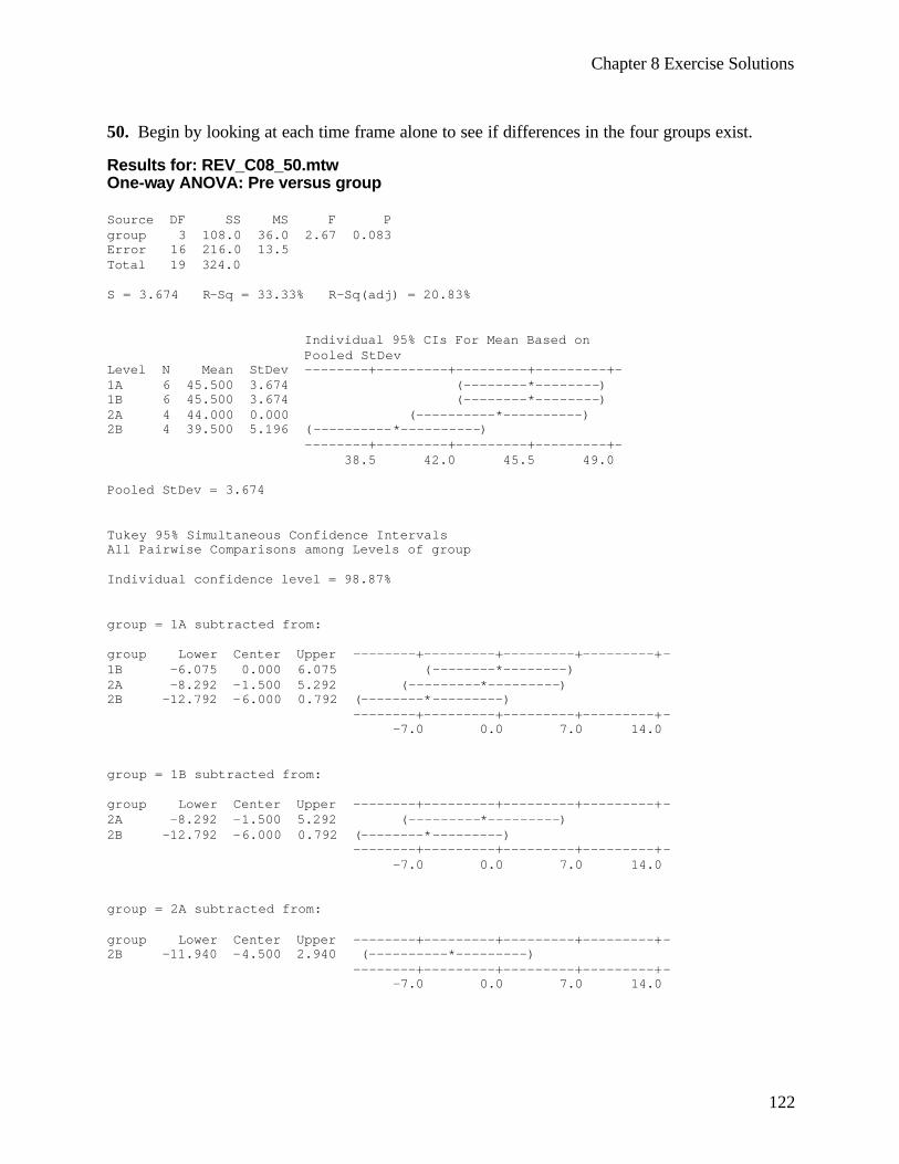
Chapter 8 Exercise Solutions
122
50. Begin by looking at each time frame alone to see if differences in the four groups exist. Results for: REV_C08_50.mtw One-way ANOVA: Pre versus group Source DF SS MS F P group 3 108.0 36.0 2.67 0.083 Error 16 216.0 13.5 Total 19 324.0 S = 3.674 R-Sq = 33.33% R-Sq(adj) = 20.83% Individual 95% CIs For Mean Based on Pooled StDev Level N Mean StDev --------+---------+---------+---------+- 1A 6 45.500 3.674 (--------*--------) 1B 6 45.500 3.674 (--------*--------) 2A 4 44.000 0.000 (----------*----------) 2B 4 39.500 5.196 (----------*----------) --------+---------+---------+---------+- 38.5 42.0 45.5 49.0 Pooled StDev = 3.674 Tukey 95% Simultaneous Confidence Intervals All Pairwise Comparisons among Levels of group Individual confidence level = 98.87% group = 1A subtracted from: group Lower Center Upper --------+---------+---------+---------+- 1B -6.075 0.000 6.075 (--------*--------) 2A -8.292 -1.500 5.292 (---------*---------) 2B -12.792 -6.000 0.792 (--------*---------) --------+---------+---------+---------+- -7.0 0.0 7.0 14.0 group = 1B subtracted from: group Lower Center Upper --------+---------+---------+---------+- 2A -8.292 -1.500 5.292 (---------*---------) 2B -12.792 -6.000 0.792 (--------*---------) --------+---------+---------+---------+- -7.0 0.0 7.0 14.0 group = 2A subtracted from: group Lower Center Upper --------+---------+---------+---------+- 2B -11.940 -4.500 2.940 (----------*---------) --------+---------+---------+---------+- -7.0 0.0 7.0 14.0
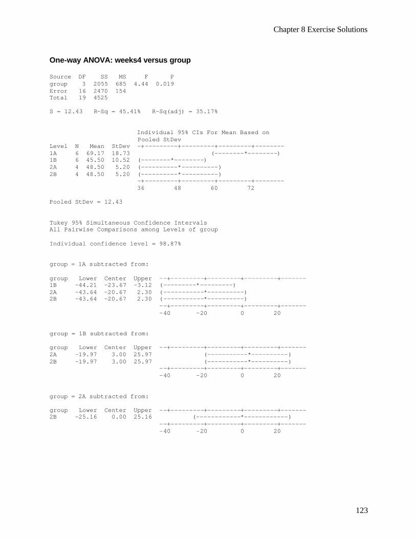
Chapter 8 Exercise Solutions
123
One-way ANOVA: weeks4 versus group Source DF SS MS F P group 3 2055 685 4.44 0.019 Error 16 2470 154 Total 19 4525 S = 12.43 R-Sq = 45.41% R-Sq(adj) = 35.17% Individual 95% CIs For Mean Based on Pooled StDev Level N Mean StDev -+---------+---------+---------+-------- 1A 6 69.17 18.73 (--------*--------) 1B 6 45.50 10.52 (--------*--------) 2A 4 48.50 5.20 (----------*----------) 2B 4 48.50 5.20 (----------*----------) -+---------+---------+---------+-------- 36 48 60 72 Pooled StDev = 12.43 Tukey 95% Simultaneous Confidence Intervals All Pairwise Comparisons among Levels of group Individual confidence level = 98.87% group = 1A subtracted from: group Lower Center Upper --+---------+---------+---------+------- 1B -44.21 -23.67 -3.12 (---------*---------) 2A -43.64 -20.67 2.30 (-----------*----------) 2B -43.64 -20.67 2.30 (-----------*----------) --+---------+---------+---------+------- -40 -20 0 20 group = 1B subtracted from: group Lower Center Upper --+---------+---------+---------+------- 2A -19.97 3.00 25.97 (-----------*----------) 2B -19.97 3.00 25.97 (-----------*----------) --+---------+---------+---------+------- -40 -20 0 20 group = 2A subtracted from: group Lower Center Upper --+---------+---------+---------+------- 2B -25.16 0.00 25.16 (------------*------------) --+---------+---------+---------+------- -40 -20 0 20
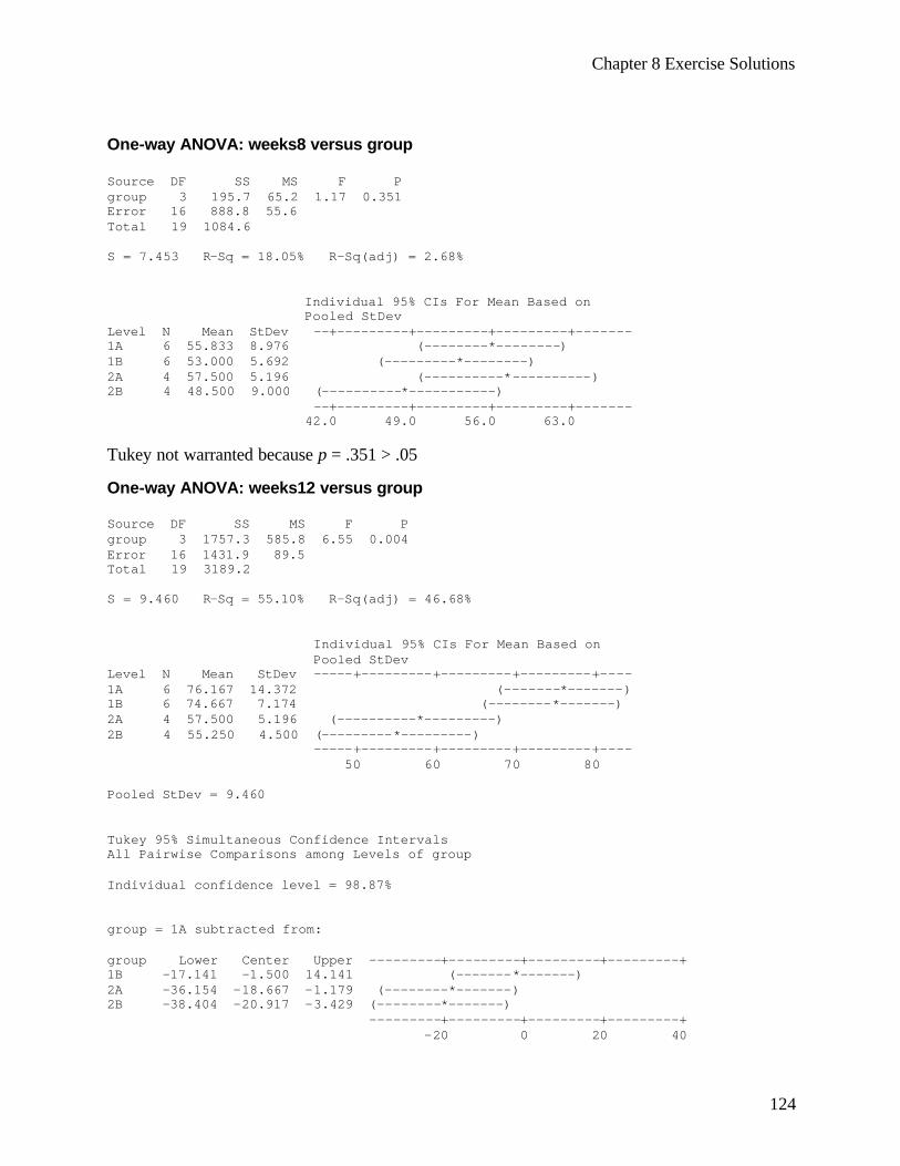
Chapter 8 Exercise Solutions
124
One-way ANOVA: weeks8 versus group Source DF SS MS F P group 3 195.7 65.2 1.17 0.351 Error 16 888.8 55.6 Total 19 1084.6 S = 7.453 R-Sq = 18.05% R-Sq(adj) = 2.68% Individual 95% CIs For Mean Based on Pooled StDev Level N Mean StDev --+---------+---------+---------+------- 1A 6 55.833 8.976 (--------*--------) 1B 6 53.000 5.692 (---------*--------) 2A 4 57.500 5.196 (----------*----------) 2B 4 48.500 9.000 (----------*-----------) --+---------+---------+---------+------- 42.0 49.0 56.0 63.0 Tukey not warranted because p = .351 > .05 One-way ANOVA: weeks12 versus group Source DF SS MS F P group 3 1757.3 585.8 6.55 0.004 Error 16 1431.9 89.5 Total 19 3189.2 S = 9.460 R-Sq = 55.10% R-Sq(adj) = 46.68% Individual 95% CIs For Mean Based on Pooled StDev Level N Mean StDev -----+---------+---------+---------+---- 1A 6 76.167 14.372 (-------*-------) 1B 6 74.667 7.174 (--------*-------) 2A 4 57.500 5.196 (----------*---------) 2B 4 55.250 4.500 (---------*---------) -----+---------+---------+---------+---- 50 60 70 80 Pooled StDev = 9.460 Tukey 95% Simultaneous Confidence Intervals All Pairwise Comparisons among Levels of group Individual confidence level = 98.87% group = 1A subtracted from: group Lower Center Upper ---------+---------+---------+---------+ 1B -17.141 -1.500 14.141 (-------*-------) 2A -36.154 -18.667 -1.179 (--------*-------) 2B -38.404 -20.917 -3.429 (--------*-------) ---------+---------+---------+---------+ -20 0 20 40
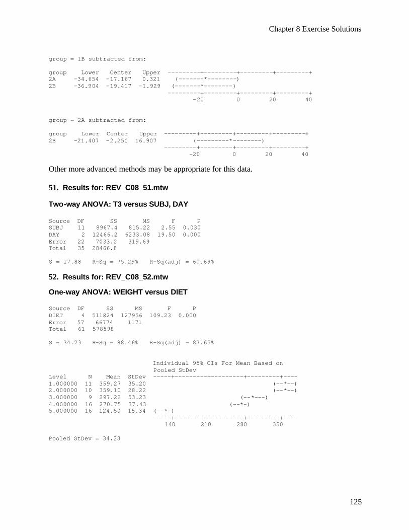
Chapter 8 Exercise Solutions
125
group = 1B subtracted from: group Lower Center Upper ---------+---------+---------+---------+ 2A -34.654 -17.167 0.321 (-------*--------) 2B -36.904 -19.417 -1.929 (-------*--------) ---------+---------+---------+---------+ -20 0 20 40 group = 2A subtracted from: group Lower Center Upper ---------+---------+---------+---------+ 2B -21.407 -2.250 16.907 (---------*--------) ---------+---------+---------+---------+ -20 0 20 40 Other more advanced methods may be appropriate for this data. 51. Results for: REV_C08_51.mtw Two-way ANOVA: T3 versus SUBJ, DAY Source DF SS MS F P SUBJ 11 8967.4 815.22 2.55 0.030 DAY 2 12466.2 6233.08 19.50 0.000 Error 22 7033.2 319.69 Total 35 28466.8 S = 17.88 R-Sq = 75.29% R-Sq(adj) = 60.69% 52. Results for: REV_C08_52.mtw One-way ANOVA: WEIGHT versus DIET Source DF SS MS F P DIET 4 511824 127956 109.23 0.000 Error 57 66774 1171 Total 61 578598 S = 34.23 R-Sq = 88.46% R-Sq(adj) = 87.65% Individual 95% CIs For Mean Based on Pooled StDev Level N Mean StDev -----+---------+---------+---------+---- 1.000000 11 359.27 35.20 (--*--) 2.000000 10 359.10 28.22 (--*--) 3.000000 9 297.22 53.23 (--*---) 4.000000 16 270.75 37.43 (--*-) 5.000000 16 124.50 15.34 (--*-) -----+---------+---------+---------+---- 140 210 280 350 Pooled StDev = 34.23
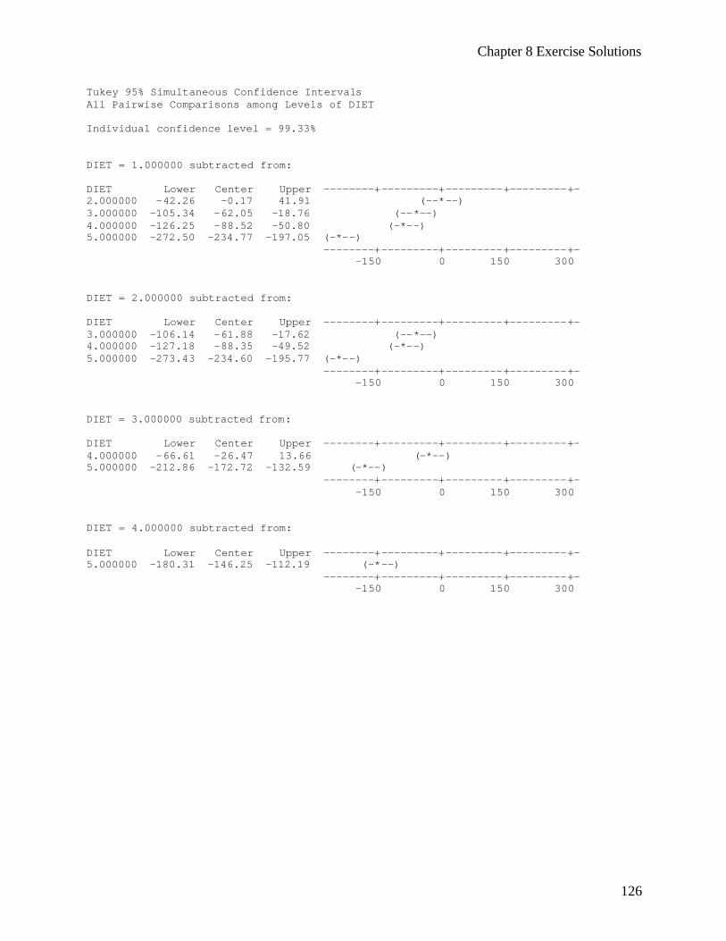
Chapter 8 Exercise Solutions
126
Tukey 95% Simultaneous Confidence Intervals All Pairwise Comparisons among Levels of DIET Individual confidence level = 99.33% DIET = 1.000000 subtracted from: DIET Lower Center Upper --------+---------+---------+---------+- 2.000000 -42.26 -0.17 41.91 (--*--) 3.000000 -105.34 -62.05 -18.76 (--*--) 4.000000 -126.25 -88.52 -50.80 (-*--) 5.000000 -272.50 -234.77 -197.05 (-*--) --------+---------+---------+---------+- -150 0 150 300 DIET = 2.000000 subtracted from: DIET Lower Center Upper --------+---------+---------+---------+- 3.000000 -106.14 -61.88 -17.62 (--*--) 4.000000 -127.18 -88.35 -49.52 (-*--) 5.000000 -273.43 -234.60 -195.77 (-*--) --------+---------+---------+---------+- -150 0 150 300 DIET = 3.000000 subtracted from: DIET Lower Center Upper --------+---------+---------+---------+- 4.000000 -66.61 -26.47 13.66 (-*--) 5.000000 -212.86 -172.72 -132.59 (-*--) --------+---------+---------+---------+- -150 0 150 300 DIET = 4.000000 subtracted from: DIET Lower Center Upper --------+---------+---------+---------+- 5.000000 -180.31 -146.25 -112.19 (-*--) --------+---------+---------+---------+- -150 0 150 300
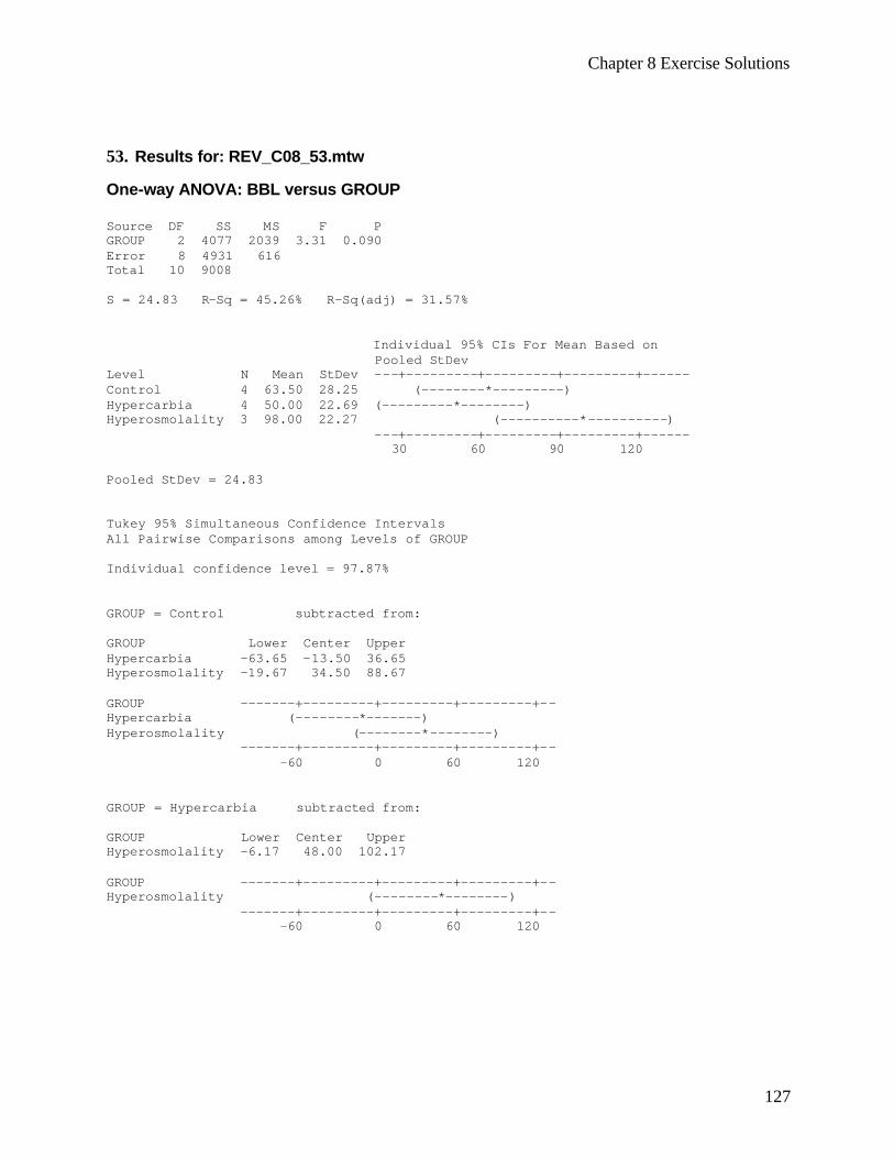
Chapter 8 Exercise Solutions
127
53. Results for: REV_C08_53.mtw One-way ANOVA: BBL versus GROUP Source DF SS MS F P GROUP 2 4077 2039 3.31 0.090 Error 8 4931 616 Total 10 9008 S = 24.83 R-Sq = 45.26% R-Sq(adj) = 31.57% Individual 95% CIs For Mean Based on Pooled StDev Level N Mean StDev ---+---------+---------+---------+------ Control 4 63.50 28.25 (--------*---------) Hypercarbia 4 50.00 22.69 (---------*--------) Hyperosmolality 3 98.00 22.27 (----------*----------) ---+---------+---------+---------+------ 30 60 90 120 Pooled StDev = 24.83 Tukey 95% Simultaneous Confidence Intervals All Pairwise Comparisons among Levels of GROUP Individual confidence level = 97.87% GROUP = Control subtracted from: GROUP Lower Center Upper Hypercarbia -63.65 -13.50 36.65 Hyperosmolality -19.67 34.50 88.67 GROUP -------+---------+---------+---------+-- Hypercarbia (--------*-------) Hyperosmolality (--------*--------) -------+---------+---------+---------+-- -60 0 60 120 GROUP = Hypercarbia subtracted from: GROUP Lower Center Upper Hyperosmolality -6.17 48.00 102.17 GROUP -------+---------+---------+---------+-- Hyperosmolality (--------*--------) -------+---------+---------+---------+-- -60 0 60 120
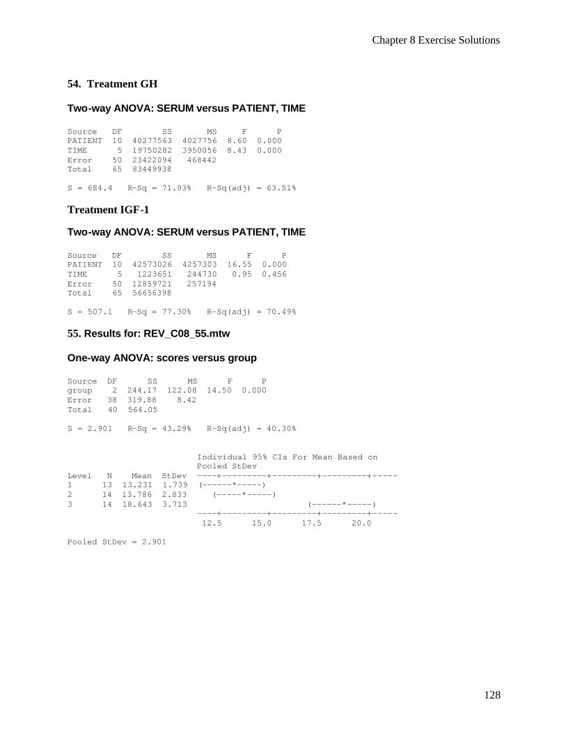
Chapter 8 Exercise Solutions
128
54. Treatment GH Two-way ANOVA: SERUM versus PATIENT, TIME Source DF SS MS F P PATIENT 10 40277563 4027756 8.60 0.000 TIME 5 19750282 3950056 8.43 0.000 Error 50 23422094 468442 Total 65 83449938 S = 684.4 R-Sq = 71.93% R-Sq(adj) = 63.51% Treatment IGF-1 Two-way ANOVA: SERUM versus PATIENT, TIME Source DF SS MS F P PATIENT 10 42573026 4257303 16.55 0.000 TIME 5 1223651 244730 0.95 0.456 Error 50 12859721 257194 Total 65 56656398 S = 507.1 R-Sq = 77.30% R-Sq(adj) = 70.49% 55. Results for: REV_C08_55.mtw One-way ANOVA: scores versus group Source DF SS MS F P group 2 244.17 122.08 14.50 0.000 Error 38 319.88 8.42 Total 40 564.05 S = 2.901 R-Sq = 43.29% R-Sq(adj) = 40.30% Individual 95% CIs For Mean Based on Pooled StDev Level N Mean StDev ----+---------+---------+---------+----- 1 13 13.231 1.739 (------*-----) 2 14 13.786 2.833 (-----*-----) 3 14 18.643 3.713 (------*-----) ----+---------+---------+---------+----- 12.5 15.0 17.5 20.0 Pooled StDev = 2.901
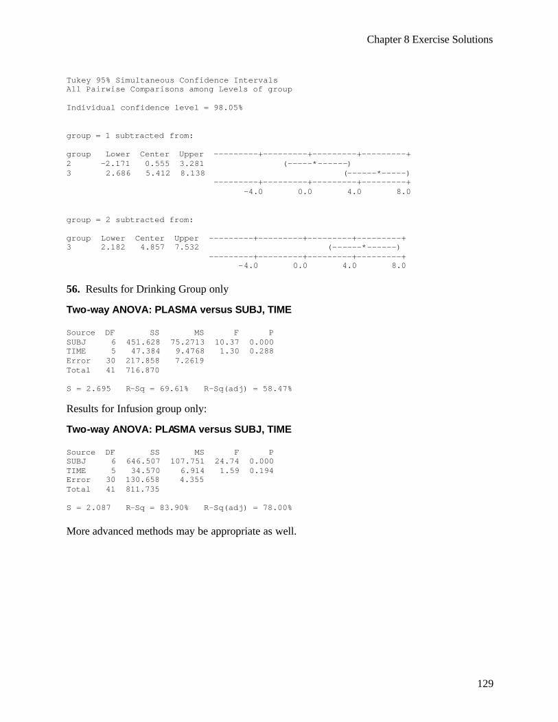
Chapter 8 Exercise Solutions
129
Tukey 95% Simultaneous Confidence Intervals All Pairwise Comparisons among Levels of group Individual confidence level = 98.05% group = 1 subtracted from: group Lower Center Upper ---------+---------+---------+---------+ 2 -2.171 0.555 3.281 (-----*------) 3 2.686 5.412 8.138 (------*-----) ---------+---------+---------+---------+ -4.0 0.0 4.0 8.0 group = 2 subtracted from: group Lower Center Upper ---------+---------+---------+---------+ 3 2.182 4.857 7.532 (------*------) ---------+---------+---------+---------+ -4.0 0.0 4.0 8.0 56. Results for Drinking Group only Two-way ANOVA: PLASMA versus SUBJ, TIME Source DF SS MS F P SUBJ 6 451.628 75.2713 10.37 0.000 TIME 5 47.384 9.4768 1.30 0.288 Error 30 217.858 7.2619 Total 41 716.870 S = 2.695 R-Sq = 69.61% R-Sq(adj) = 58.47% Results for Infusion group only: Two-way ANOVA: PLASMA versus SUBJ, TIME Source DF SS MS F P SUBJ 6 646.507 107.751 24.74 0.000 TIME 5 34.570 6.914 1.59 0.194 Error 30 130.658 4.355 Total 41 811.735 S = 2.087 R-Sq = 83.90% R-Sq(adj) = 78.00% More advanced methods may be appropriate as well.
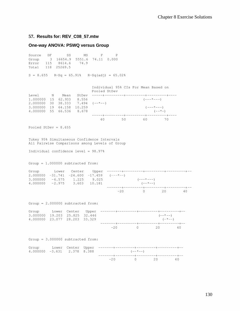
Chapter 8 Exercise Solutions
130
57. Results for: REV_C08_57.mtw One-way ANOVA: PSWQ versus Group Source DF SS MS F P Group 3 16654.9 5551.6 74.11 0.000 Error 115 8614.6 74.9 Total 118 25269.5 S = 8.655 R-Sq = 65.91% R-Sq(adj) = 65.02% Individual 95% CIs For Mean Based on Pooled StDev Level N Mean StDev -----+---------+---------+---------+---- 1.000000 15 62.933 8.556 (---*---) 2.000000 30 38.333 7.494 (--*--) 3.000000 19 64.158 10.259 (---*---) 4.000000 55 66.536 8.678 (--*-) -----+---------+---------+---------+---- 40 50 60 70 Pooled StDev = 8.655 Tukey 95% Simultaneous Confidence Intervals All Pairwise Comparisons among Levels of Group Individual confidence level = 98.97% Group = 1.000000 subtracted from: Group Lower Center Upper -------+---------+---------+---------+-- 2.000000 -31.741 -24.600 -17.459 (---*--) 3.000000 -6.575 1.225 9.025 (---*---) 4.000000 -2.975 3.603 10.181 (--*--) -------+---------+---------+---------+-- -20 0 20 40 Group = 2.000000 subtracted from: Group Lower Center Upper -------+---------+---------+---------+-- 3.000000 19.203 25.825 32.446 (--*--) 4.000000 23.077 28.203 33.329 (-*--) -------+---------+---------+---------+-- -20 0 20 40 Group = 3.000000 subtracted from: Group Lower Center Upper -------+---------+---------+---------+-- 4.000000 -3.631 2.378 8.388 (--*--) -------+---------+---------+---------+-- -20 0 20 40
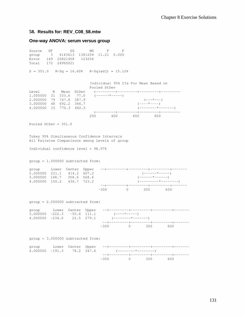
Chapter 8 Exercise Solutions
131
58. Results for: REV_C08_58.mtw One-way ANOVA: serum versus group Source DF SS MS F P group 3 4143613 1381204 11.21 0.000 Error 169 20821408 123204 Total 172 24965021 S = 351.0 R-Sq = 16.60% R-Sq(adj) = 15.12% Individual 95% CIs For Mean Based on Pooled StDev Level N Mean StDev +---------+---------+---------+--------- 1.000000 31 333.6 77.0 (------*-----) 2.000000 79 747.8 387.9 (---*---) 3.000000 48 692.2 346.7 (----*----) 4.000000 15 770.3 482.5 (--------*-------) +---------+---------+---------+--------- 200 400 600 800 Pooled StDev = 351.0 Tukey 95% Simultaneous Confidence Intervals All Pairwise Comparisons among Levels of group Individual confidence level = 98.97% group = 1.000000 subtracted from: group Lower Center Upper --+---------+---------+---------+------- 2.000000 221.1 414.2 607.2 (------*-----) 3.000000 148.7 358.6 568.4 (------*------) 4.000000 150.2 436.7 723.2 (---------*--------) --+---------+---------+---------+------- -300 0 300 600 group = 2.000000 subtracted from: group Lower Center Upper --+---------+---------+---------+------- 3.000000 -222.3 -55.6 111.1 (----*-----) 4.000000 -234.0 22.5 279.1 (--------*-------) --+---------+---------+---------+------- -300 0 300 600 group = 3.000000 subtracted from: group Lower Center Upper --+---------+---------+---------+------- 4.000000 -191.3 78.2 347.6 (--------*--------) --+---------+---------+---------+------- -300 0 300 600
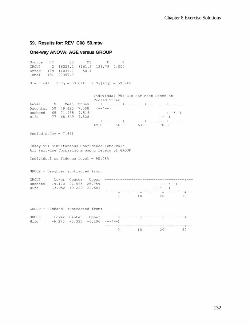
Chapter 8 Exercise Solutions
132
59. Results for: REV_C08_59.mtw One-way ANOVA: AGE versus GROUP Source DF SS MS F P GROUP 2 16323.2 8161.6 139.79 0.000 Error 189 11034.7 58.4 Total 191 27357.9 S = 7.641 R-Sq = 59.67% R-Sq(adj) = 59.24% Individual 95% CIs For Mean Based on Pooled StDev Level N Mean StDev --+---------+---------+---------+------- Daughter 50 49.420 7.508 (--*--) Husband 65 71.985 7.516 (--*--) Wife 77 68.649 7.828 (-*--) --+---------+---------+---------+------- 49.0 56.0 63.0 70.0 Pooled StDev = 7.641 Tukey 95% Simultaneous Confidence Intervals All Pairwise Comparisons among Levels of GROUP Individual confidence level = 98.08% GROUP = Daughter subtracted from: GROUP Lower Center Upper ------+---------+---------+---------+--- Husband 19.170 22.565 25.959 (---*--) Wife 15.952 19.229 22.507 (--*---) ------+---------+---------+---------+--- 0 10 20 30 GROUP = Husband subtracted from: GROUP Lower Center Upper ------+---------+---------+---------+--- Wife -6.375 -3.335 -0.296 (--*--) ------+---------+---------+---------+--- 0 10 20 30
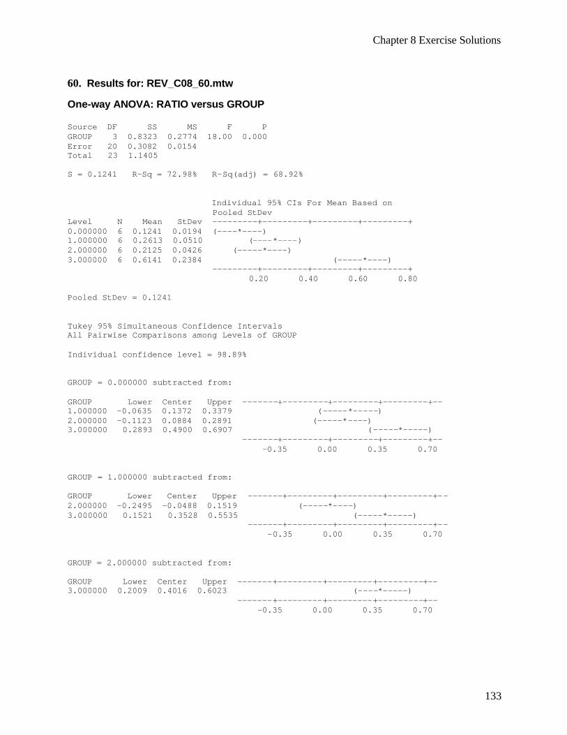
Chapter 8 Exercise Solutions
133
60. Results for: REV_C08_60.mtw One-way ANOVA: RATIO versus GROUP Source DF SS MS F P GROUP 3 0.8323 0.2774 18.00 0.000 Error 20 0.3082 0.0154 Total 23 1.1405 S = 0.1241 R-Sq = 72.98% R-Sq(adj) = 68.92% Individual 95% CIs For Mean Based on Pooled StDev Level N Mean StDev ---------+---------+---------+---------+ 0.000000 6 0.1241 0.0194 (----*----) 1.000000 6 0.2613 0.0510 (----*----) 2.000000 6 0.2125 0.0426 (-----*----) 3.000000 6 0.6141 0.2384 (-----*----) ---------+---------+---------+---------+ 0.20 0.40 0.60 0.80 Pooled StDev = 0.1241 Tukey 95% Simultaneous Confidence Intervals All Pairwise Comparisons among Levels of GROUP Individual confidence level = 98.89% GROUP = 0.000000 subtracted from: GROUP Lower Center Upper -------+---------+---------+---------+-- 1.000000 -0.0635 0.1372 0.3379 (-----*-----) 2.000000 -0.1123 0.0884 0.2891 (-----*----) 3.000000 0.2893 0.4900 0.6907 (-----*-----) -------+---------+---------+---------+-- -0.35 0.00 0.35 0.70 GROUP = 1.000000 subtracted from: GROUP Lower Center Upper -------+---------+---------+---------+-- 2.000000 -0.2495 -0.0488 0.1519 (-----*----) 3.000000 0.1521 0.3528 0.5535 (-----*-----) -------+---------+---------+---------+-- -0.35 0.00 0.35 0.70 GROUP = 2.000000 subtracted from: GROUP Lower Center Upper -------+---------+---------+---------+-- 3.000000 0.2009 0.4016 0.6023 (----*-----) -------+---------+---------+---------+-- -0.35 0.00 0.35 0.70

Chapter 8 Exercise Solutions
134
61. Results for: REV_C08_61.mtw SAP = serum alkaline phosphatase level One-way ANOVA: SAP versus GRADE Source DF SS MS F P GRADE 2 36181 18091 5.55 0.009 Error 29 94560 3261 Total 31 130742 S = 57.10 R-Sq = 27.67% R-Sq(adj) = 22.69% Individual 95% CIs For Mean Based on Pooled StDev Level N Mean StDev +---------+---------+---------+--------- I 9 118.00 61.85 (--------*---------) II 8 143.63 55.90 (---------*---------) III 15 194.80 54.82 (-------*------) +---------+---------+---------+--------- 80 120 160 200 Pooled StDev = 57.10 Tukey 95% Simultaneous Confidence Intervals All Pairwise Comparisons among Levels of GRADE Individual confidence level = 98.03% GRADE = I subtracted from: GRADE Lower Center Upper ------+---------+---------+---------+--- II -42.85 25.63 94.10 (---------*--------) III 17.38 76.80 136.22 (--------*-------) ------+---------+---------+---------+--- -70 0 70 140 GRADE = II subtracted from: GRADE Lower Center Upper ------+---------+---------+---------+--- III -10.52 51.18 112.87 (--------*--------) ------+---------+---------+---------+--- -70 0 70 140
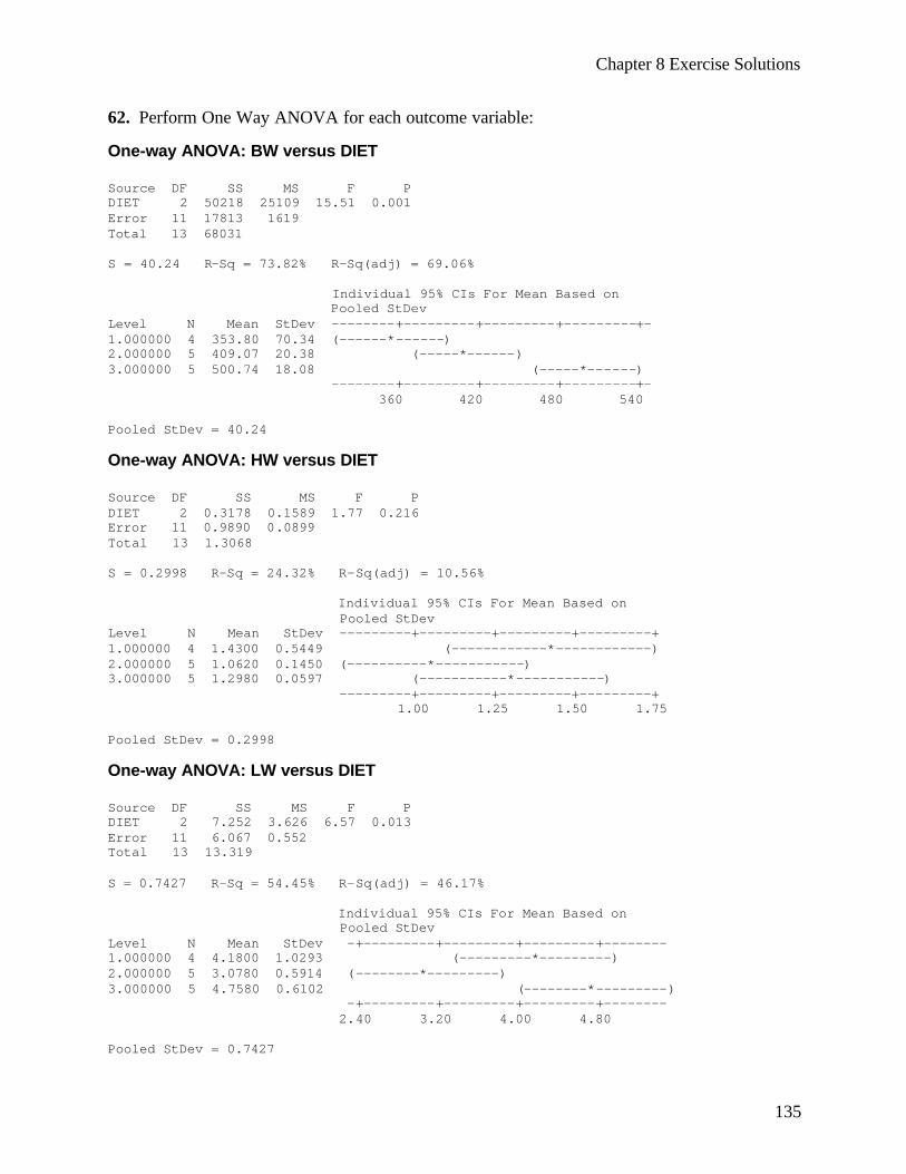
Chapter 8 Exercise Solutions
135
62. Perform One Way ANOVA for each outcome variable: One-way ANOVA: BW versus DIET Source DF SS MS F P DIET 2 50218 25109 15.51 0.001 Error 11 17813 1619 Total 13 68031 S = 40.24 R-Sq = 73.82% R-Sq(adj) = 69.06% Individual 95% CIs For Mean Based on Pooled StDev Level N Mean StDev --------+---------+---------+---------+- 1.000000 4 353.80 70.34 (------*------) 2.000000 5 409.07 20.38 (-----*------) 3.000000 5 500.74 18.08 (-----*------) --------+---------+---------+---------+- 360 420 480 540 Pooled StDev = 40.24 One-way ANOVA: HW versus DIET Source DF SS MS F P DIET 2 0.3178 0.1589 1.77 0.216 Error 11 0.9890 0.0899 Total 13 1.3068 S = 0.2998 R-Sq = 24.32% R-Sq(adj) = 10.56% Individual 95% CIs For Mean Based on Pooled StDev Level N Mean StDev ---------+---------+---------+---------+ 1.000000 4 1.4300 0.5449 (------------*------------) 2.000000 5 1.0620 0.1450 (----------*-----------) 3.000000 5 1.2980 0.0597 (-----------*-----------) ---------+---------+---------+---------+ 1.00 1.25 1.50 1.75 Pooled StDev = 0.2998 One-way ANOVA: LW versus DIET Source DF SS MS F P DIET 2 7.252 3.626 6.57 0.013 Error 11 6.067 0.552 Total 13 13.319 S = 0.7427 R-Sq = 54.45% R-Sq(adj) = 46.17% Individual 95% CIs For Mean Based on Pooled StDev Level N Mean StDev -+---------+---------+---------+-------- 1.000000 4 4.1800 1.0293 (---------*---------) 2.000000 5 3.0780 0.5914 (--------*---------) 3.000000 5 4.7580 0.6102 (--------*---------) -+---------+---------+---------+-------- 2.40 3.20 4.00 4.80 Pooled StDev = 0.7427
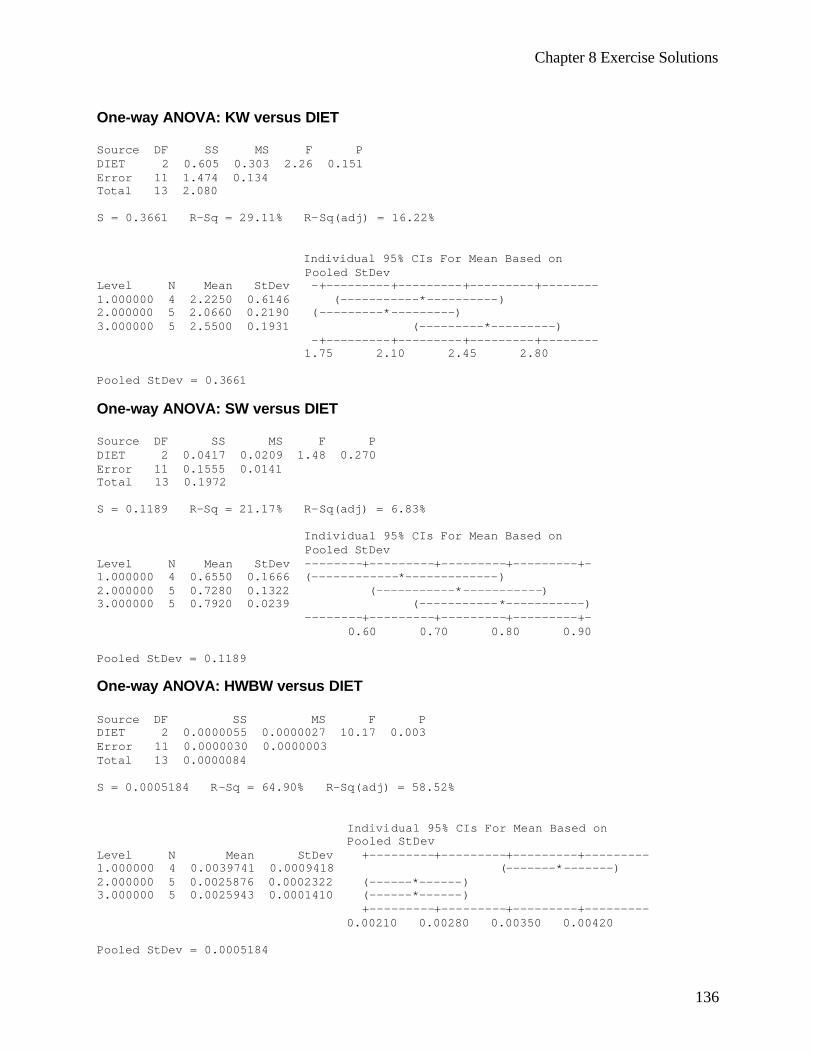
Chapter 8 Exercise Solutions
136
One-way ANOVA: KW versus DIET Source DF SS MS F P DIET 2 0.605 0.303 2.26 0.151 Error 11 1.474 0.134 Total 13 2.080 S = 0.3661 R-Sq = 29.11% R-Sq(adj) = 16.22% Individual 95% CIs For Mean Based on Pooled StDev Level N Mean StDev -+---------+---------+---------+-------- 1.000000 4 2.2250 0.6146 (-----------*----------) 2.000000 5 2.0660 0.2190 (---------*---------) 3.000000 5 2.5500 0.1931 (---------*---------) -+---------+---------+---------+-------- 1.75 2.10 2.45 2.80 Pooled StDev = 0.3661 One-way ANOVA: SW versus DIET Source DF SS MS F P DIET 2 0.0417 0.0209 1.48 0.270 Error 11 0.1555 0.0141 Total 13 0.1972 S = 0.1189 R-Sq = 21.17% R-Sq(adj) = 6.83% Individual 95% CIs For Mean Based on Pooled StDev Level N Mean StDev --------+---------+---------+---------+- 1.000000 4 0.6550 0.1666 (------------*-------------) 2.000000 5 0.7280 0.1322 (-----------*-----------) 3.000000 5 0.7920 0.0239 (-----------*-----------) --------+---------+---------+---------+- 0.60 0.70 0.80 0.90 Pooled StDev = 0.1189 One-way ANOVA: HWBW versus DIET Source DF SS MS F P DIET 2 0.0000055 0.0000027 10.17 0.003 Error 11 0.0000030 0.0000003 Total 13 0.0000084 S = 0.0005184 R-Sq = 64.90% R-Sq(adj) = 58.52% Individual 95% CIs For Mean Based on Pooled StDev Level N Mean StDev +---------+---------+---------+--------- 1.000000 4 0.0039741 0.0009418 (-------*-------) 2.000000 5 0.0025876 0.0002322 (------*------) 3.000000 5 0.0025943 0.0001410 (------*------) +---------+---------+---------+--------- 0.00210 0.00280 0.00350 0.00420 Pooled StDev = 0.0005184

Chapter 8 Exercise Solutions
137
One-way ANOVA: LWBW versus DIET Source DF SS MS F P DIET 2 0.0000417 0.0000209 9.52 0.004 Error 11 0.0000241 0.0000022 Total 13 0.0000658 S = 0.001480 R-Sq = 63.38% R-Sq(adj) = 56.72% Individual 95% CIs For Mean Based on Pooled StDev Level N Mean StDev +---------+---------+---------+--------- 1.000000 4 0.011825 0.001924 (-------*-------) 2.000000 5 0.007495 0.001155 (------*-------) 3.000000 5 0.009523 0.001384 (-------*------) +---------+---------+---------+--------- 0.0060 0.0080 0.0100 0.0120 Pooled StDev = 0.001480 One-way ANOVA: KWBW versus DIET Source DF SS MS F P DIET 2 0.0000040 0.0000020 6.99 0.011 Error 11 0.0000032 0.0000003 Total 13 0.0000072 S = 0.0005356 R-Sq = 55.97% R-Sq(adj) = 47.96% Individual 95% CIs For Mean Based on Pooled StDev Level N Mean StDev -----+---------+---------+---------+---- 1.000000 4 0.0062508 0.0008643 (---------*---------) 2.000000 5 0.0050417 0.0003353 (--------*--------) 3.000000 5 0.0050923 0.0003407 (--------*--------) -----+---------+---------+---------+---- 0.00480 0.00540 0.00600 0.00660 Pooled StDev = 0.0005356 One-way ANOVA: SWBW versus DIET Source DF SS MS F P DIET 2 0.0000002 0.0000001 1.60 0.245 Error 11 0.0000006 0.0000001 Total 13 0.0000007 S = 0.0002242 R-Sq = 22.54% R-Sq(adj) = 8.45% Individual 95% CIs For Mean Based on Pooled StDev Level N Mean StDev --+---------+---------+---------+------- 1.000000 4 0.0018322 0.0001461 (------------*-----------) 2.000000 5 0.0017816 0.0003356 (----------*----------) 3.000000 5 0.0015844 0.0000980 (----------*----------) --+---------+---------+---------+------- 0.00140 0.00160 0.00180 0.00200 Pooled StDev = 0.0002242
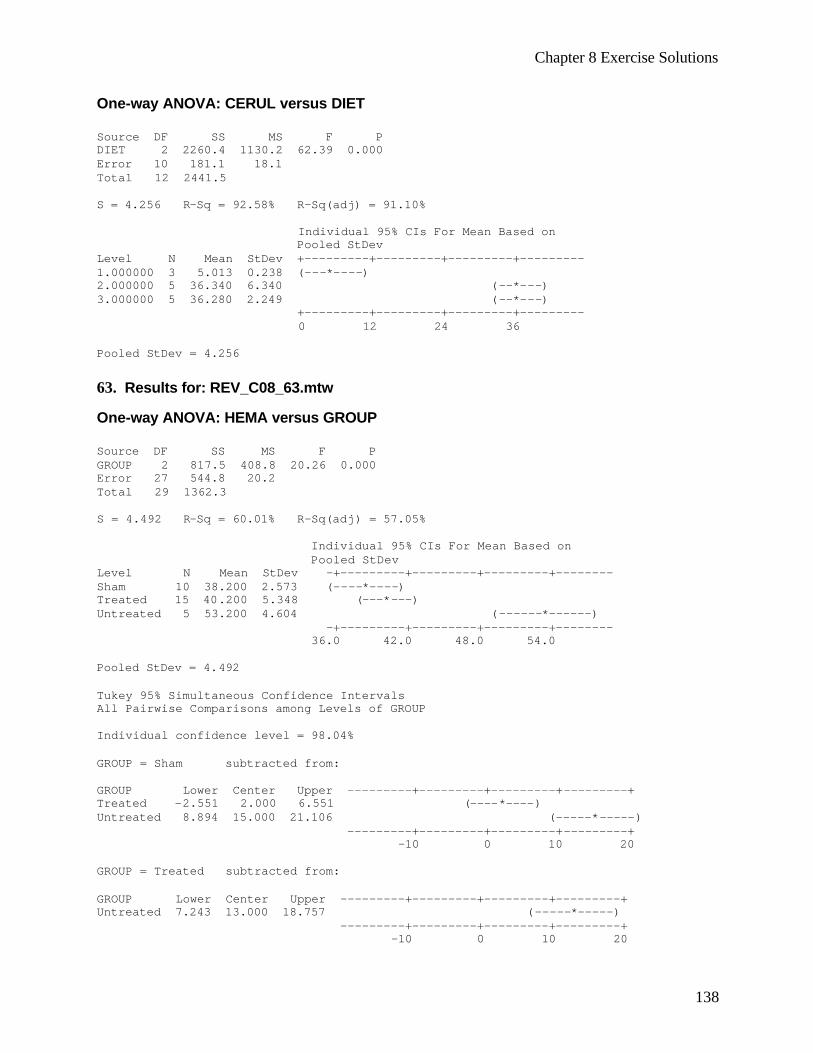
Chapter 8 Exercise Solutions
138
One-way ANOVA: CERUL versus DIET Source DF SS MS F P DIET 2 2260.4 1130.2 62.39 0.000 Error 10 181.1 18.1 Total 12 2441.5 S = 4.256 R-Sq = 92.58% R-Sq(adj) = 91.10% Individual 95% CIs For Mean Based on Pooled StDev Level N Mean StDev +---------+---------+---------+--------- 1.000000 3 5.013 0.238 (---*----) 2.000000 5 36.340 6.340 (--*---) 3.000000 5 36.280 2.249 (--*---) +---------+---------+---------+--------- 0 12 24 36 Pooled StDev = 4.256 63. Results for: REV_C08_63.mtw One-way ANOVA: HEMA versus GROUP Source DF SS MS F P GROUP 2 817.5 408.8 20.26 0.000 Error 27 544.8 20.2 Total 29 1362.3 S = 4.492 R-Sq = 60.01% R-Sq(adj) = 57.05% Individual 95% CIs For Mean Based on Pooled StDev Level N Mean StDev -+---------+---------+---------+-------- Sham 10 38.200 2.573 (----*----) Treated 15 40.200 5.348 (---*---) Untreated 5 53.200 4.604 (------*------) -+---------+---------+---------+-------- 36.0 42.0 48.0 54.0 Pooled StDev = 4.492 Tukey 95% Simultaneous Confidence Intervals All Pairwise Comparisons among Levels of GROUP Individual confidence level = 98.04% GROUP = Sham subtracted from: GROUP Lower Center Upper ---------+---------+---------+---------+ Treated -2.551 2.000 6.551 (----*----) Untreated 8.894 15.000 21.106 (-----*-----) ---------+---------+---------+---------+ -10 0 10 20 GROUP = Treated subtracted from: GROUP Lower Center Upper ---------+---------+---------+---------+ Untreated 7.243 13.000 18.757 (-----*-----) ---------+---------+---------+---------+ -10 0 10 20
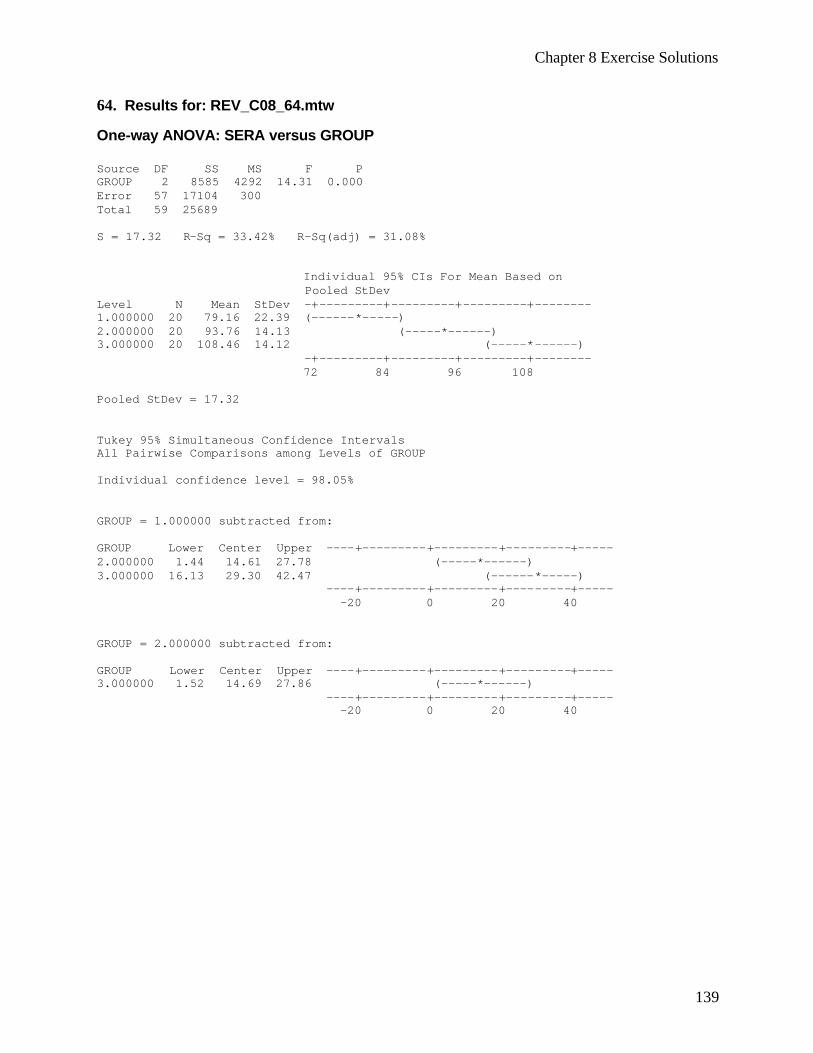
Chapter 8 Exercise Solutions
139
64. Results for: REV_C08_64.mtw One-way ANOVA: SERA versus GROUP Source DF SS MS F P GROUP 2 8585 4292 14.31 0.000 Error 57 17104 300 Total 59 25689 S = 17.32 R-Sq = 33.42% R-Sq(adj) = 31.08% Individual 95% CIs For Mean Based on Pooled StDev Level N Mean StDev -+---------+---------+---------+-------- 1.000000 20 79.16 22.39 (------*-----) 2.000000 20 93.76 14.13 (-----*------) 3.000000 20 108.46 14.12 (-----*------) -+---------+---------+---------+-------- 72 84 96 108 Pooled StDev = 17.32 Tukey 95% Simultaneous Confidence Intervals All Pairwise Comparisons among Levels of GROUP Individual confidence level = 98.05% GROUP = 1.000000 subtracted from: GROUP Lower Center Upper ----+---------+---------+---------+----- 2.000000 1.44 14.61 27.78 (-----*------) 3.000000 16.13 29.30 42.47 (------*-----) ----+---------+---------+---------+----- -20 0 20 40 GROUP = 2.000000 subtracted from: GROUP Lower Center Upper ----+---------+---------+---------+----- 3.000000 1.52 14.69 27.86 (-----*------) ----+---------+---------+---------+----- -20 0 20 40
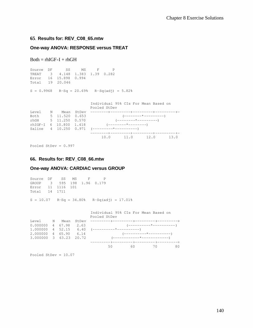
Chapter 8 Exercise Solutions
140
65. Results for: REV_C08_65.mtw One-way ANOVA: RESPONSE versus TREAT Both = rhIGF-I + rhGH Source DF SS MS F P TREAT 3 4.148 1.383 1.39 0.282 Error 16 15.898 0.994 Total 19 20.046 S = 0.9968 R-Sq = 20.69% R-Sq(adj) = 5.82% Individual 95% CIs For Mean Based on Pooled StDev Level N Mean StDev --------+---------+---------+---------+- Both 5 11.520 0.653 (--------*---------) rhGH 5 11.250 0.570 (--------*---------) rhIGF-I 6 10.800 1.418 (--------*--------) Saline 4 10.250 0.971 (---------*----------) --------+---------+---------+---------+- 10.0 11.0 12.0 13.0 Pooled StDev = 0.997 66. Results for: REV_C08_66.mtw One-way ANOVA: CARDIAC versus GROUP Source DF SS MS F P GROUP 3 595 198 1.96 0.179 Error 11 1116 101 Total 14 1711 S = 10.07 R-Sq = 34.80% R-Sq(adj) = 17.01% Individual 95% CIs For Mean Based on Pooled StDev Level N Mean StDev ---------+---------+---------+---------+ 0.000000 4 67.98 2.63 (----------*----------) 1.000000 4 52.15 6.40 (----------*----------) 2.000000 4 65.90 6.14 (----------*----------) 3.000000 3 63.23 20.72 (------------*------------) ---------+---------+---------+---------+ 50 60 70 80 Pooled StDev = 10.07
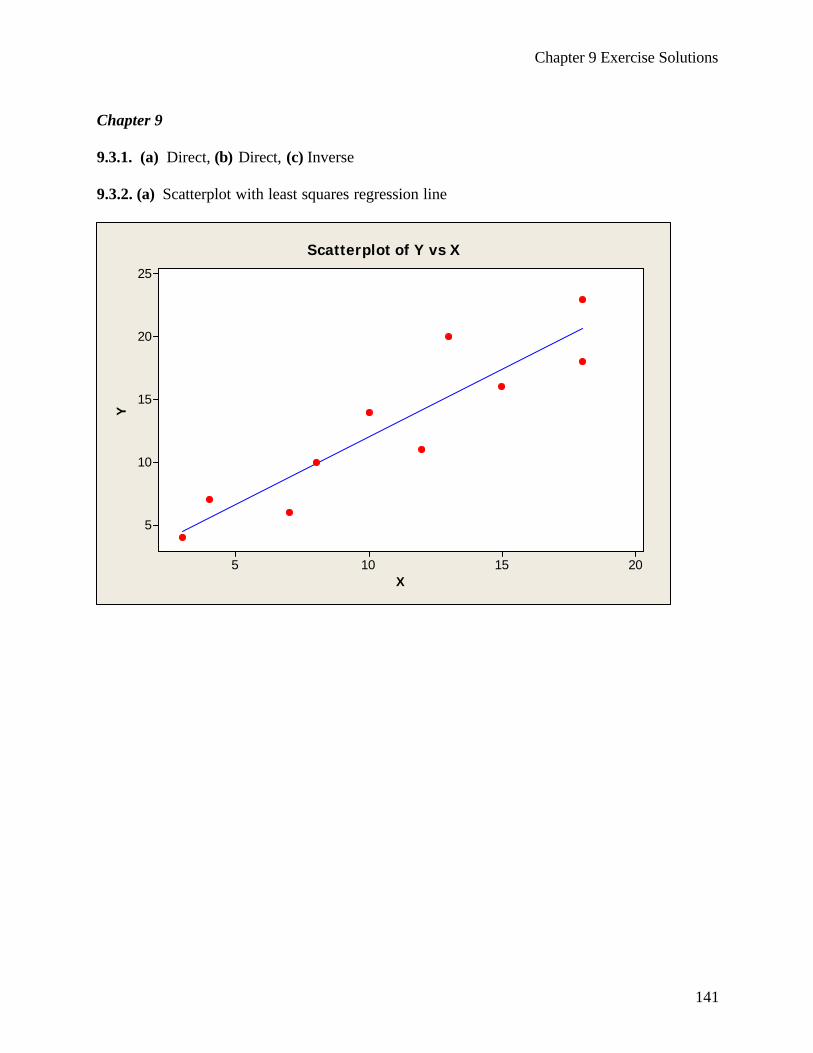
Chapter 9 Exercise Solutions
141
Chapter 9 9.3.1. (a) Direct, (b) Direct, (c) Inverse 9.3.2. (a) Scatterplot with least squares regression line
X
Y
2015105
25
20
15
10
5
Scatterplot of Y vs X
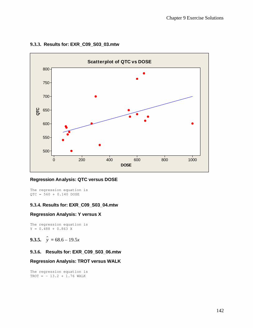
Chapter 9 Exercise Solutions
142
9.3.3. Results for: EXR_C09_S03_03.mtw
DOSE
QTC
10008006004002000
800
750
700
650
600
550
500
Scatterplot of QTC vs DOSE
Regression Analysis: QTC versus DOSE The regression equation is QTC = 560 + 0.140 DOSE 9.3.4. Results for: EXR_C09_S03_04.mtw Regression Analysis: Y versus X The regression equation is Y = 0.488 + 0.863 X
9.3.5. $y = 68.6 – 19.5x 9.3.6. Results for: EXR_C09_S03_06.mtw Regression Analysis: TROT versus WALK The regression equation is TROT = - 13.2 + 1.76 WALK
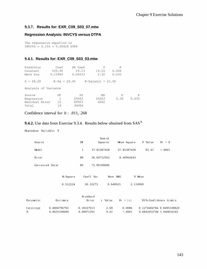
Chapter 9 Exercise Solutions
143
9.3.7. Results for: EXR_C09_S03_07.mtw Regression Analysis: INVCYS versus DTPA The regression equation is INVCYS = 0.193 + 0.00628 DTPA 9.4.1. Results for: EXR_C09_S03_03.mtw Predictor Coef SE Coef T P Constant 559.90 29.13 19.22 0.000 Meth Dos 0.13989 0.06033 2.32 0.035 S = 68.28 R-Sq = 26.4% R-Sq(adj) = 21.5% Analysis of Variance Source DF SS MS F P Regression 1 25063 25063 5.38 0.035 Residual Error 15 69923 4662 Total 16 94986 Confidence interval for β : .011, .268 9.4.2. Use data from Exercise 9.3.4. Results below obtained from SAS® Dependent Variable: Y Sum of Source DF Squares Mean Square F Value Pr > F Model 1 37.85387438 37.85387438 92.41 <.0001 Error 88 36.04712562 0.40962643 Corrected Total 89 73.90100000 R-Square Coeff Var Root MSE Y Mean 0.512224 30.33273 0.640021 2.110000 Standard Parameter Estimate Error t Value Pr > |t| 95% Confidence Limits Intercept 0.4884796793 0.18167013 2.69 0.0086 0.1274484766 0.8495108820 X 0.8625108089 0.08972291 9.61 <.0001 0.6842053746 1.040816243
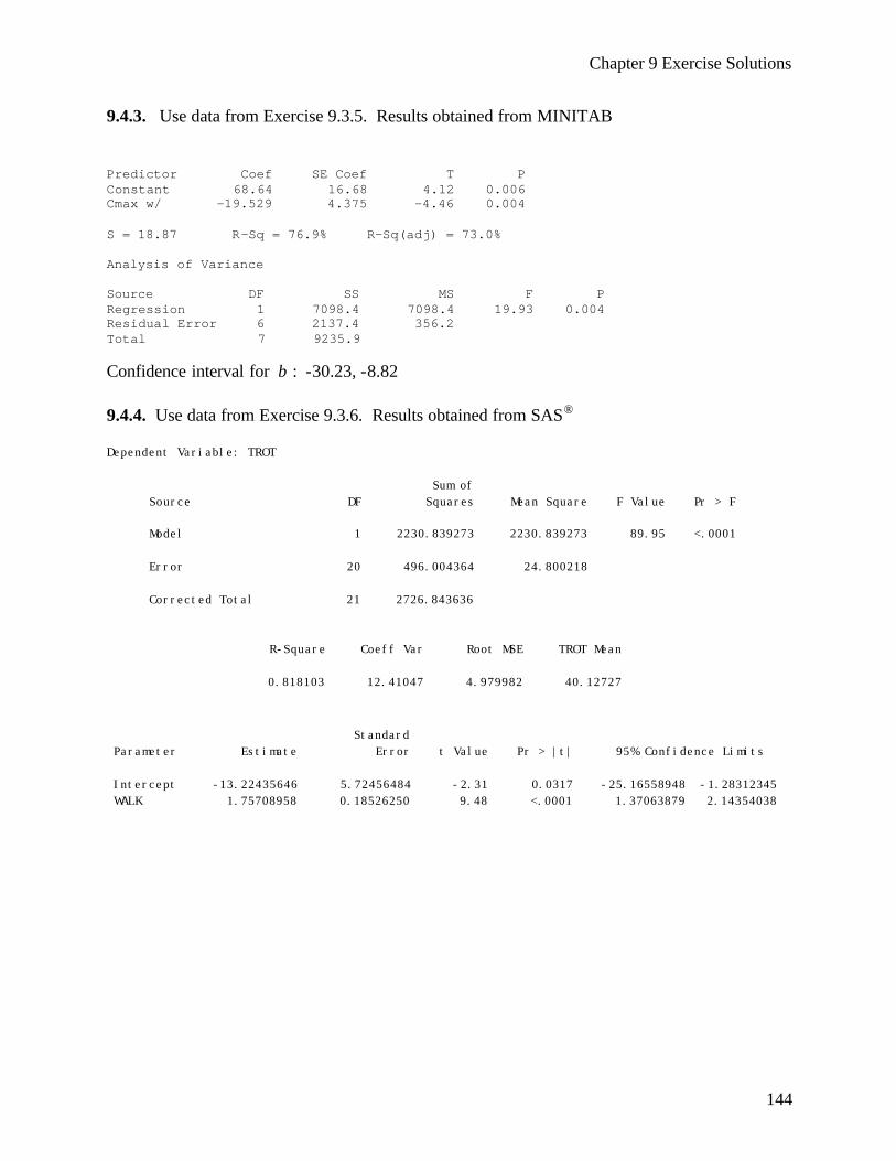
Chapter 9 Exercise Solutions
144
9.4.3. Use data from Exercise 9.3.5. Results obtained from MINITAB Predictor Coef SE Coef T P Constant 68.64 16.68 4.12 0.006 Cmax w/ -19.529 4.375 -4.46 0.004 S = 18.87 R-Sq = 76.9% R-Sq(adj) = 73.0% Analysis of Variance Source DF SS MS F P Regression 1 7098.4 7098.4 19.93 0.004 Residual Error 6 2137.4 356.2 Total 7 9235.9 Confidence interval for β : -30.23, -8.82 9.4.4. Use data from Exercise 9.3.6. Results obtained from SAS® Dependent Variable: TROT Sum of Source DF Squares Mean Square F Value Pr > F Model 1 2230.839273 2230.839273 89.95 <.0001 Error 20 496.004364 24.800218 Corrected Total 21 2726.843636 R-Square Coeff Var Root MSE TROT Mean 0.818103 12.41047 4.979982 40.12727 Standard Parameter Estimate Error t Value Pr > |t| 95% Confidence Limits Intercept -13.22435646 5.72456484 -2.31 0.0317 -25.16558948 -1.28312345 WALK 1.75708958 0.18526250 9.48 <.0001 1.37063879 2.14354038
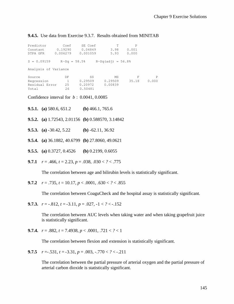
Chapter 9 Exercise Solutions
145
9.4.5. Use data from Exercise 9.3.7. Results obtained from MINITAB Predictor Coef SE Coef T P Constant 0.19290 0.04849 3.98 0.001 DTPA GFR 0.006279 0.001059 5.93 0.000 S = 0.09159 R-Sq = 58.5% R-Sq(adj) = 56.8% Analysis of Variance Source DF SS MS F P Regression 1 0.29509 0.29509 35.18 0.000 Residual Error 25 0.20972 0.00839 Total 26 0.50481 Confidence interval for β : 0.0041, 0.0085 9.5.1. (a) 580.6, 651.2 (b) 466.1, 765.6 9.5.2. (a) 1.72543, 2.01156 (b) 0.588570, 3.14842 9.5.3. (a) -30.42, 5.22 (b) -62.11, 36.92 9.5.4. (a) 36.1882, 40.6799 (b) 27.8060, 49.0621 9.5.5. (a) 0.3727, 0.4526 (b) 0.2199, 0.6055 9.7.1 r = .466, t = 2.23, p = .038, .030 < ? < .775
The correlation between age and bilirubin levels is statistically significant.
9.7.2 r = .735, t = 10.17, p < .0001, .630 < ? < .855
The correlation between CoaguCheck and the hospital assay is statistically significant. 9.7.3. r = -.812, t = -3.11, p = .027, -1 < ? < -.152
The correlation between AUC levels when taking water and when taking grapefruit juice is statistically significant.
9.7.4. r = .882, t = 7.4938, p < .0001, .721 < ? < 1
The correlation between flexion and extension is statistically significant.
9.7.5 r =-.531, t = -3.31, p = .003, -.770 < ? < -.211
The correlation between the partial pressure of arterial oxygen and the partial pressure of arterial carbon dioxide is statistically significant.
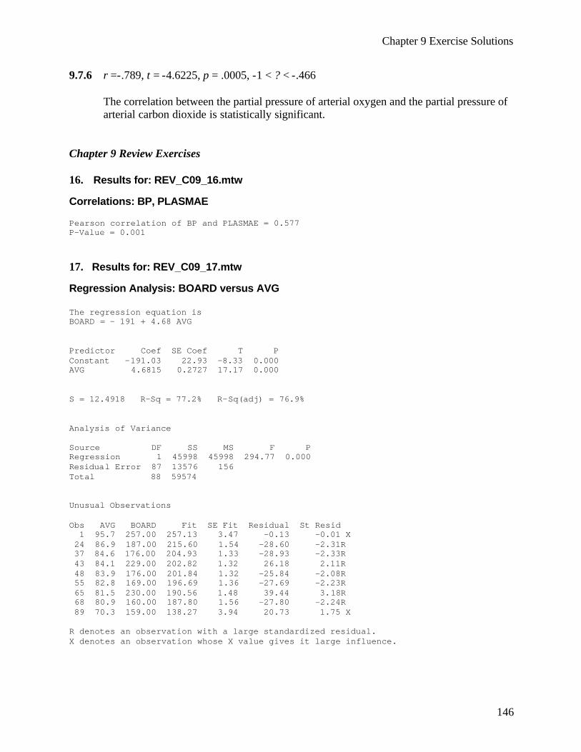
Chapter 9 Exercise Solutions
146
9.7.6 r =-.789, t = -4.6225, p = .0005, -1 < ? < -.466
The correlation between the partial pressure of arterial oxygen and the partial pressure of arterial carbon dioxide is statistically significant.
Chapter 9 Review Exercises 16. Results for: REV_C09_16.mtw Correlations: BP, PLASMAE Pearson correlation of BP and PLASMAE = 0.577 P-Value = 0.001 17. Results for: REV_C09_17.mtw Regression Analysis: BOARD versus AVG The regression equation is BOARD = - 191 + 4.68 AVG Predictor Coef SE Coef T P Constant -191.03 22.93 -8.33 0.000 AVG 4.6815 0.2727 17.17 0.000 S = 12.4918 R-Sq = 77.2% R-Sq(adj) = 76.9% Analysis of Variance Source DF SS MS F P Regression 1 45998 45998 294.77 0.000 Residual Error 87 13576 156 Total 88 59574 Unusual Observations Obs AVG BOARD Fit SE Fit Residual St Resid 1 95.7 257.00 257.13 3.47 -0.13 -0.01 X 24 86.9 187.00 215.60 1.54 -28.60 -2.31R 37 84.6 176.00 204.93 1.33 -28.93 -2.33R 43 84.1 229.00 202.82 1.32 26.18 2.11R 48 83.9 176.00 201.84 1.32 -25.84 -2.08R 55 82.8 169.00 196.69 1.36 -27.69 -2.23R 65 81.5 230.00 190.56 1.48 39.44 3.18R 68 80.9 160.00 187.80 1.56 -27.80 -2.24R 89 70.3 159.00 138.27 3.94 20.73 1.75 X R denotes an observation with a large standardized residual. X denotes an observation whose X value gives it large influence.
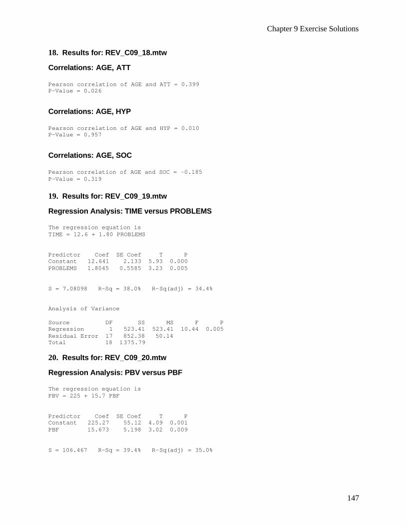
Chapter 9 Exercise Solutions
147
18. Results for: REV_C09_18.mtw Correlations: AGE, ATT Pearson correlation of AGE and ATT = 0.399 P-Value = 0.026 Correlations: AGE, HYP Pearson correlation of AGE and HYP = 0.010 P-Value = 0.957 Correlations: AGE, SOC Pearson correlation of AGE and SOC = -0.185 P-Value = 0.319 19. Results for: REV_C09_19.mtw Regression Analysis: TIME versus PROBLEMS The regression equation is TIME = 12.6 + 1.80 PROBLEMS Predictor Coef SE Coef T P Constant 12.641 2.133 5.93 0.000 PROBLEMS 1.8045 0.5585 3.23 0.005 S = 7.08098 R-Sq = 38.0% R-Sq(adj) = 34.4% Analysis of Variance Source DF SS MS F P Regression 1 523.41 523.41 10.44 0.005 Residual Error 17 852.38 50.14 Total 18 1375.79 20. Results for: REV_C09_20.mtw Regression Analysis: PBV versus PBF The regression equation is PBV = 225 + 15.7 PBF Predictor Coef SE Coef T P Constant 225.27 55.12 4.09 0.001 PBF 15.673 5.198 3.02 0.009 S = 106.467 R-Sq = 39.4% R-Sq(adj) = 35.0%
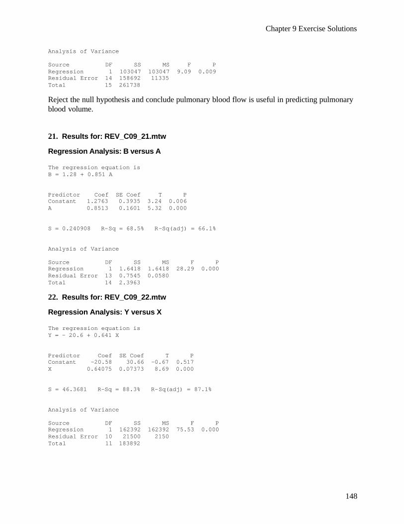
Chapter 9 Exercise Solutions
148
Analysis of Variance Source DF SS MS F P Regression 1 103047 103047 9.09 0.009 Residual Error 14 158692 11335 Total 15 261738 Reject the null hypothesis and conclude pulmonary blood flow is useful in predicting pulmonary blood volume. 21. Results for: REV_C09_21.mtw Regression Analysis: B versus A The regression equation is B = 1.28 + 0.851 A Predictor Coef SE Coef T P Constant 1.2763 0.3935 3.24 0.006 A 0.8513 0.1601 5.32 0.000 S = 0.240908 R-Sq = 68.5% R-Sq(adj) = 66.1% Analysis of Variance Source DF SS MS F P Regression 1 1.6418 1.6418 28.29 0.000 Residual Error 13 0.7545 0.0580 Total 14 2.3963 22. Results for: REV_C09_22.mtw Regression Analysis: Y versus X The regression equation is Y = - 20.6 + 0.641 X Predictor Coef SE Coef T P Constant -20.58 30.66 -0.67 0.517 X 0.64075 0.07373 8.69 0.000 S = 46.3681 R-Sq = 88.3% R-Sq(adj) = 87.1% Analysis of Variance Source DF SS MS F P Regression 1 162392 162392 75.53 0.000 Residual Error 10 21500 2150 Total 11 183892
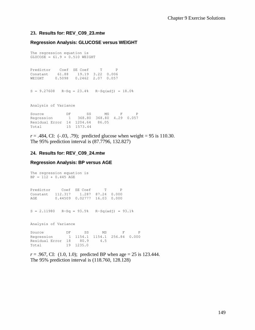
Chapter 9 Exercise Solutions
149
23. Results for: REV_C09_23.mtw Regression Analysis: GLUCOSE versus WEIGHT The regression equation is GLUCOSE = 61.9 + 0.510 WEIGHT Predictor Coef SE Coef T P Constant 61.88 19.19 3.22 0.006 WEIGHT 0.5098 0.2462 2.07 0.057 S = 9.27608 R-Sq = 23.4% R-Sq(adj) = 18.0% Analysis of Variance Source DF SS MS F P Regression 1 368.80 368.80 4.29 0.057 Residual Error 14 1204.64 86.05 Total 15 1573.44 r = .484, CI: (-.03, .79); predicted glucose when weight = 95 is 110.30. The 95% prediction interval is (87.7796, 132.827) 24. Results for: REV_C09_24.mtw Regression Analysis: BP versus AGE The regression equation is BP = 112 + 0.445 AGE Predictor Coef SE Coef T P Constant 112.317 1.287 87.24 0.000 AGE 0.44509 0.02777 16.03 0.000 S = 2.11980 R-Sq = 93.5% R-Sq(adj) = 93.1% Analysis of Variance Source DF SS MS F P Regression 1 1154.1 1154.1 256.84 0.000 Residual Error 18 80.9 4.5 Total 19 1235.0 r = .967, CI: (1.0, 1.0); predicted BP when age = 25 is 123.444. The 95% prediction interval is (118.760, 128.128)
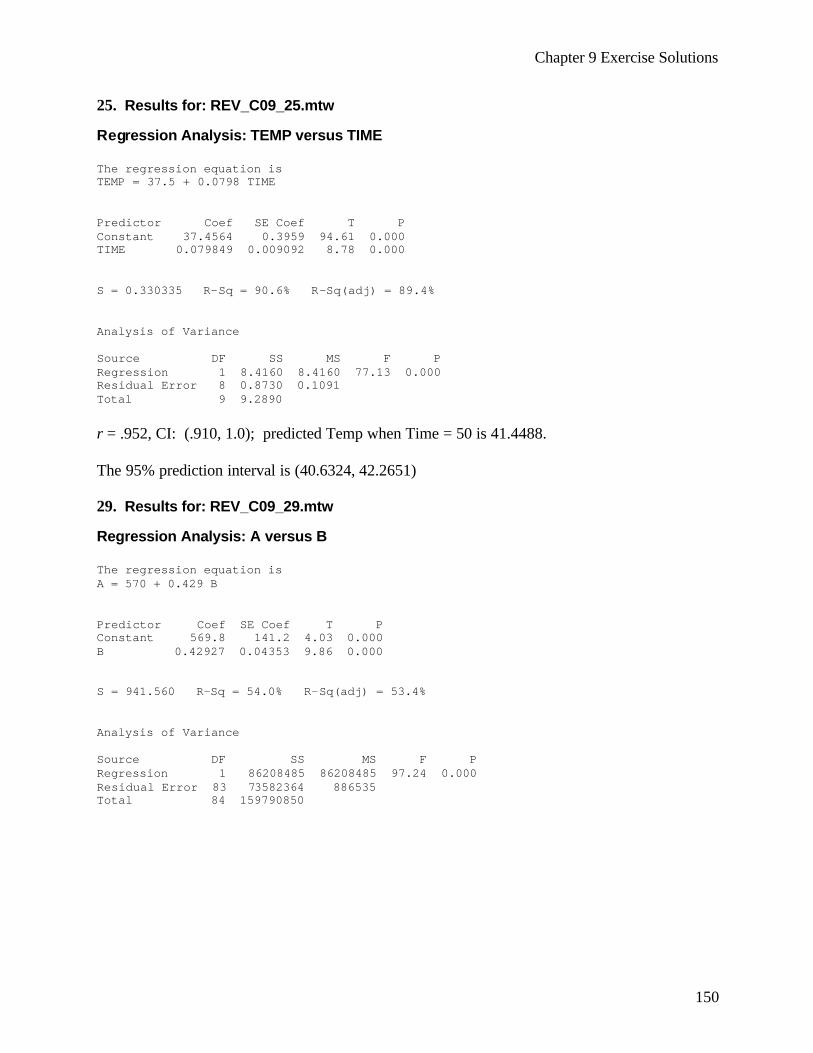
Chapter 9 Exercise Solutions
150
25. Results for: REV_C09_25.mtw Regression Analysis: TEMP versus TIME The regression equation is TEMP = 37.5 + 0.0798 TIME Predictor Coef SE Coef T P Constant 37.4564 0.3959 94.61 0.000 TIME 0.079849 0.009092 8.78 0.000 S = 0.330335 R-Sq = 90.6% R-Sq(adj) = 89.4% Analysis of Variance Source DF SS MS F P Regression 1 8.4160 8.4160 77.13 0.000 Residual Error 8 0.8730 0.1091 Total 9 9.2890 r = .952, CI: (.910, 1.0); predicted Temp when Time = 50 is 41.4488. The 95% prediction interval is (40.6324, 42.2651) 29. Results for: REV_C09_29.mtw Regression Analysis: A versus B The regression equation is A = 570 + 0.429 B Predictor Coef SE Coef T P Constant 569.8 141.2 4.03 0.000 B 0.42927 0.04353 9.86 0.000 S = 941.560 R-Sq = 54.0% R-Sq(adj) = 53.4% Analysis of Variance Source DF SS MS F P Regression 1 86208485 86208485 97.24 0.000 Residual Error 83 73582364 886535 Total 84 159790850
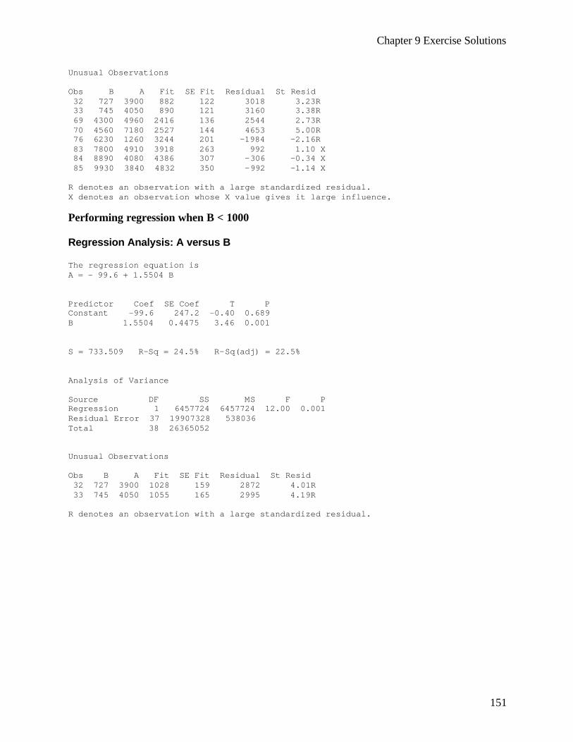
Chapter 9 Exercise Solutions
151
Unusual Observations Obs B A Fit SE Fit Residual St Resid 32 727 3900 882 122 3018 3.23R 33 745 4050 890 121 3160 3.38R 69 4300 4960 2416 136 2544 2.73R 70 4560 7180 2527 144 4653 5.00R 76 6230 1260 3244 201 -1984 -2.16R 83 7800 4910 3918 263 992 1.10 X 84 8890 4080 4386 307 -306 -0.34 X 85 9930 3840 4832 350 -992 -1.14 X R denotes an observation with a large standardized residual. X denotes an observation whose X value gives it large influence. Performing regression when B < 1000 Regression Analysis: A versus B The regression equation is A = - 99.6 + 1.5504 B Predictor Coef SE Coef T P Constant -99.6 247.2 -0.40 0.689 B 1.5504 0.4475 3.46 0.001 S = 733.509 R-Sq = 24.5% R-Sq(adj) = 22.5% Analysis of Variance Source DF SS MS F P Regression 1 6457724 6457724 12.00 0.001 Residual Error 37 19907328 538036 Total 38 26365052 Unusual Observations Obs B A Fit SE Fit Residual St Resid 32 727 3900 1028 159 2872 4.01R 33 745 4050 1055 165 2995 4.19R R denotes an observation with a large standardized residual.
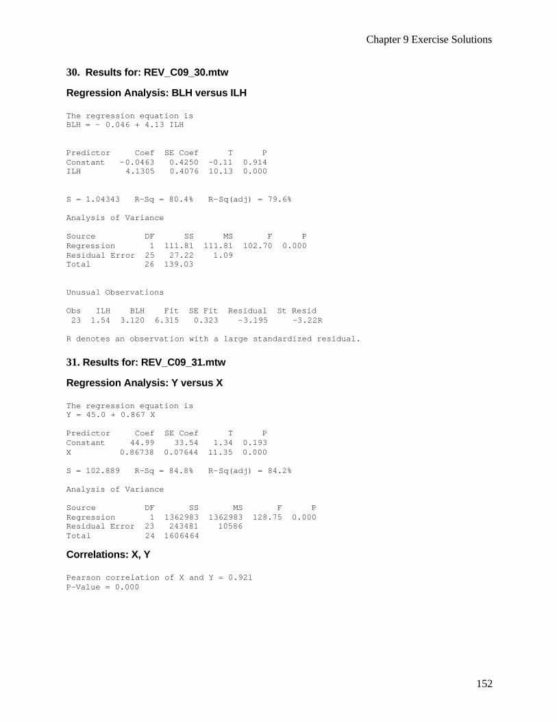
Chapter 9 Exercise Solutions
152
30. Results for: REV_C09_30.mtw Regression Analysis: BLH versus ILH The regression equation is BLH = - 0.046 + 4.13 ILH Predictor Coef SE Coef T P Constant -0.0463 0.4250 -0.11 0.914 ILH 4.1305 0.4076 10.13 0.000 S = 1.04343 R-Sq = 80.4% R-Sq(adj) = 79.6% Analysis of Variance Source DF SS MS F P Regression 1 111.81 111.81 102.70 0.000 Residual Error 25 27.22 1.09 Total 26 139.03 Unusual Observations Obs ILH BLH Fit SE Fit Residual St Resid 23 1.54 3.120 6.315 0.323 -3.195 -3.22R R denotes an observation with a large standardized residual. 31. Results for: REV_C09_31.mtw Regression Analysis: Y versus X The regression equation is Y = 45.0 + 0.867 X Predictor Coef SE Coef T P Constant 44.99 33.54 1.34 0.193 X 0.86738 0.07644 11.35 0.000 S = 102.889 R-Sq = 84.8% R-Sq(adj) = 84.2% Analysis of Variance Source DF SS MS F P Regression 1 1362983 1362983 128.75 0.000 Residual Error 23 243481 10586 Total 24 1606464 Correlations: X, Y Pearson correlation of X and Y = 0.921 P-Value = 0.000
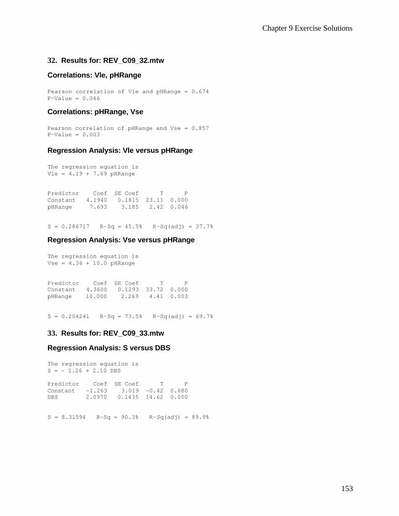
Chapter 9 Exercise Solutions
153
32. Results for: REV_C09_32.mtw Correlations: Vle, pHRange Pearson correlation of Vle and pHRange = 0.674 P-Value = 0.046 Correlations: pHRange, Vse Pearson correlation of pHRange and Vse = 0.857 P-Value = 0.003 Regression Analysis: Vle versus pHRange The regression equation is Vle = 4.19 + 7.69 pHRange Predictor Coef SE Coef T P Constant 4.1940 0.1815 23.11 0.000 pHRange 7.693 3.185 2.42 0.046 S = 0.286717 R-Sq = 45.5% R-Sq(adj) = 37.7% Regression Analysis: Vse versus pHRange The regression equation is Vse = 4.36 + 10.0 pHRange Predictor Coef SE Coef T P Constant 4.3600 0.1293 33.72 0.000 pHRange 10.000 2.269 4.41 0.003 S = 0.204241 R-Sq = 73.5% R-Sq(adj) = 69.7% 33. Results for: REV_C09_33.mtw Regression Analysis: S versus DBS The regression equation is S = - 1.26 + 2.10 DBS Predictor Coef SE Coef T P Constant -1.263 3.019 -0.42 0.680 DBS 2.0970 0.1435 14.62 0.000 S = 8.31594 R-Sq = 90.3% R-Sq(adj) = 89.9%
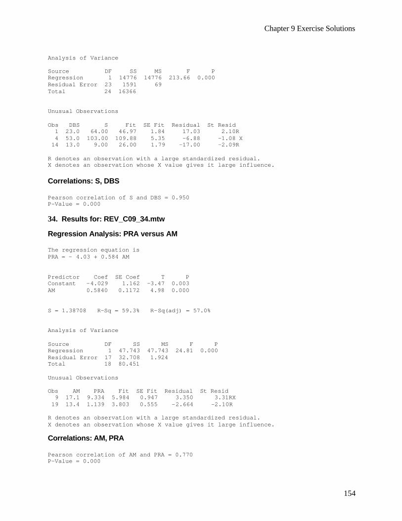
Chapter 9 Exercise Solutions
154
Analysis of Variance Source DF SS MS F P Regression 1 14776 14776 213.66 0.000 Residual Error 23 1591 69 Total 24 16366 Unusual Observations Obs DBS S Fit SE Fit Residual St Resid 1 23.0 64.00 46.97 1.84 17.03 2.10R 4 53.0 103.00 109.88 5.35 -6.88 -1.08 X 14 13.0 9.00 26.00 1.79 -17.00 -2.09R R denotes an observation with a large standardized residual. X denotes an observation whose X value gives it large influence. Correlations: S, DBS Pearson correlation of S and DBS = 0.950 P-Value = 0.000 34. Results for: REV_C09_34.mtw Regression Analysis: PRA versus AM The regression equation is PRA = - 4.03 + 0.584 AM Predictor Coef SE Coef T P Constant -4.029 1.162 -3.47 0.003 AM 0.5840 0.1172 4.98 0.000 S = 1.38708 R-Sq = 59.3% R-Sq(adj) = 57.0% Analysis of Variance Source DF SS MS F P Regression 1 47.743 47.743 24.81 0.000 Residual Error 17 32.708 1.924 Total 18 80.451 Unusual Observations Obs AM PRA Fit SE Fit Residual St Resid 9 17.1 9.334 5.984 0.947 3.350 3.31RX 19 13.4 1.139 3.803 0.555 -2.664 -2.10R R denotes an observation with a large standardized residual. X denotes an observation whose X value gives it large influence. Correlations: AM, PRA Pearson correlation of AM and PRA = 0.770 P-Value = 0.000
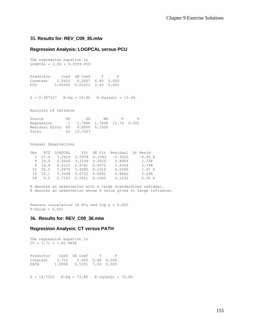
Chapter 9 Exercise Solutions
155
35. Results for: REV_C09_35.mtw Regression Analysis: LOGPCAL versus PCU The regression equation is LOGPCAL = 2.06 + 0.0559 PCU Predictor Coef SE Coef T P Constant 2.0603 0.3007 6.85 0.000 PCU 0.05593 0.01631 3.43 0.001 S = 0.387317 R-Sq = 16.4% R-Sq(adj) = 15.0% Analysis of Variance Source DF SS MS F P Regression 1 1.7648 1.7648 11.76 0.001 Residual Error 60 9.0009 0.1500 Total 61 10.7657 Unusual Observations Obs PCU LOGPCAL Fit SE Fit Residual St Resid 3 27.4 3.2918 3.5938 0.1583 -0.3020 -0.85 X 8 19.0 4.0200 3.1246 0.0510 0.8954 2.33R 9 16.4 4.4125 2.9781 0.0572 1.4344 3.74R 15 25.0 3.9975 3.4585 0.1214 0.5390 1.47 X 19 18.1 3.9394 3.0732 0.0492 0.8662 2.25R 58 9.5 2.7143 2.5911 0.1502 0.1232 0.35 X R denotes an observation with a large standardized residual. X denotes an observation whose X value gives it large influence. Pearson correlation of PCu and log y = 0.405 P-Value = 0.001 36. Results for: REV_C09_36.mtw Regression Analysis: CT versus PATH The regression equation is CT = 3.71 + 1.00 PATH Predictor Coef SE Coef T P Constant 3.712 5.492 0.68 0.506 PATH 1.0008 0.1301 7.69 0.000 S = 14.7203 R-Sq = 73.8% R-Sq(adj) = 72.6%
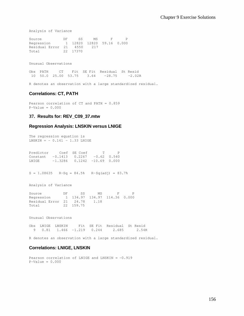
Chapter 9 Exercise Solutions
156
Analysis of Variance Source DF SS MS F P Regression 1 12820 12820 59.16 0.000 Residual Error 21 4550 217 Total 22 17370 Unusual Observations Obs PATH CT Fit SE Fit Residual St Resid 10 50.0 25.00 53.75 3.64 -28.75 -2.02R R denotes an observation with a large standardized residual. Correlations: CT, PATH Pearson correlation of CT and PATH = 0.859 P-Value = 0.000 37. Results for: REV_C09_37.mtw Regression Analysis: LNSKIN versus LNIGE The regression equation is LNSKIN = - 0.141 - 1.33 LNIGE Predictor Coef SE Coef T P Constant -0.1413 0.2267 -0.62 0.540 LNIGE -1.3286 0.1242 -10.69 0.000 S = 1.08635 R-Sq = 84.5% R-Sq(adj) = 83.7% Analysis of Variance Source DF SS MS F P Regression 1 134.97 134.97 114.36 0.000 Residual Error 21 24.78 1.18 Total 22 159.75 Unusual Observations Obs LNIGE LNSKIN Fit SE Fit Residual St Resid 9 0.81 1.466 -1.219 0.244 2.685 2.54R R denotes an observation with a large standardized residual. Correlations: LNIGE, LNSKIN Pearson correlation of LNIGE and LNSKIN = -0.919 P-Value = 0.000
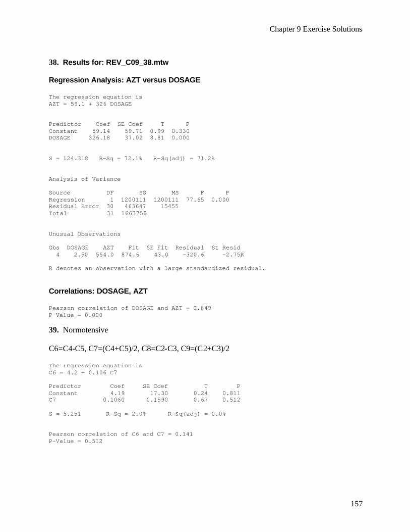
Chapter 9 Exercise Solutions
157
38. Results for: REV_C09_38.mtw Regression Analysis: AZT versus DOSAGE The regression equation is AZT = 59.1 + 326 DOSAGE Predictor Coef SE Coef T P Constant 59.14 59.71 0.99 0.330 DOSAGE 326.18 37.02 8.81 0.000 S = 124.318 R-Sq = 72.1% R-Sq(adj) = 71.2% Analysis of Variance Source DF SS MS F P Regression 1 1200111 1200111 77.65 0.000 Residual Error 30 463647 15455 Total 31 1663758 Unusual Observations Obs DOSAGE AZT Fit SE Fit Residual St Resid 4 2.50 554.0 874.6 43.0 -320.6 -2.75R R denotes an observation with a large standardized residual. Correlations: DOSAGE, AZT Pearson correlation of DOSAGE and AZT = 0.849 P-Value = 0.000 39. Normotensive C6=C4-C5, C7=(C4+C5)/2, C8=C2-C3, C9=(C2+C3)/2 The regression equation is C6 = 4.2 + 0.106 C7 Predictor Coef SE Coef T P Constant 4.19 17.30 0.24 0.811 C7 0.1060 0.1590 0.67 0.512 S = 5.251 R-Sq = 2.0% R-Sq(adj) = 0.0% Pearson correlation of C6 and C7 = 0.141 P-Value = 0.512
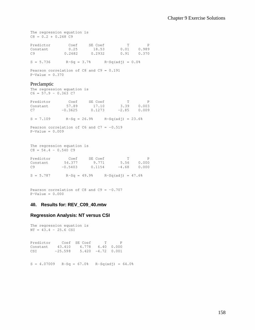
Chapter 9 Exercise Solutions
158
The regression equation is C8 = 0.2 + 0.268 C9 Predictor Coef SE Coef T P Constant 0.25 18.53 0.01 0.989 C9 0.2682 0.2932 0.91 0.370 S = 5.736 R-Sq = 3.7% R-Sq(adj) = 0.0% Pearson correlation of C8 and C9 = 0.191 P-Value = 0.370 Preclamptic The regression equation is C6 = 57.9 - 0.363 C7 Predictor Coef SE Coef T P Constant 57.89 17.10 3.39 0.003 C7 -0.3625 0.1273 -2.85 0.009 S = 7.109 R-Sq = 26.9% R-Sq(adj) = 23.6% Pearson correlation of C6 and C7 = -0.519 P-Value = 0.009 The regression equation is C8 = 54.4 - 0.540 C9 Predictor Coef SE Coef T P Constant 54.377 9.771 5.56 0.000 C9 -0.5403 0.1154 -4.68 0.000 S = 5.787 R-Sq = 49.9% R-Sq(adj) = 47.6% Pearson correlation of C8 and C9 = -0.707 P-Value = 0.000 40. Results for: REV_C09_40.mtw Regression Analysis: NT versus CSI The regression equation is NT = 43.4 - 25.6 CSI Predictor Coef SE Coef T P Constant 43.410 6.778 6.40 0.000 CSI -25.598 5.420 -4.72 0.001 S = 4.07009 R-Sq = 67.0% R-Sq(adj) = 64.0%
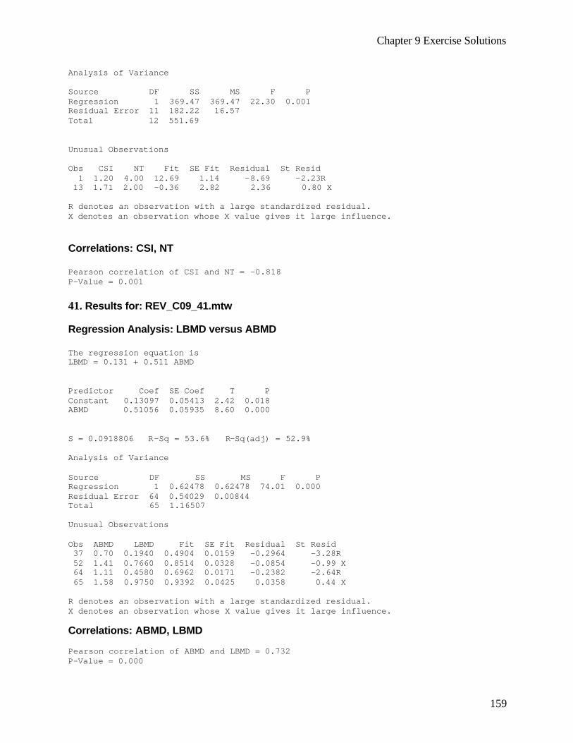
Chapter 9 Exercise Solutions
159
Analysis of Variance Source DF SS MS F P Regression 1 369.47 369.47 22.30 0.001 Residual Error 11 182.22 16.57 Total 12 551.69 Unusual Observations Obs CSI NT Fit SE Fit Residual St Resid 1 1.20 4.00 12.69 1.14 -8.69 -2.23R 13 1.71 2.00 -0.36 2.82 2.36 0.80 X R denotes an observation with a large standardized residual. X denotes an observation whose X value gives it large influence. Correlations: CSI, NT Pearson correlation of CSI and NT = -0.818 P-Value = 0.001 41. Results for: REV_C09_41.mtw Regression Analysis: LBMD versus ABMD The regression equation is LBMD = 0.131 + 0.511 ABMD Predictor Coef SE Coef T P Constant 0.13097 0.05413 2.42 0.018 ABMD 0.51056 0.05935 8.60 0.000 S = 0.0918806 R-Sq = 53.6% R-Sq(adj) = 52.9% Analysis of Variance Source DF SS MS F P Regression 1 0.62478 0.62478 74.01 0.000 Residual Error 64 0.54029 0.00844 Total 65 1.16507 Unusual Observations Obs ABMD LBMD Fit SE Fit Residual St Resid 37 0.70 0.1940 0.4904 0.0159 -0.2964 -3.28R 52 1.41 0.7660 0.8514 0.0328 -0.0854 -0.99 X 64 1.11 0.4580 0.6962 0.0171 -0.2382 -2.64R 65 1.58 0.9750 0.9392 0.0425 0.0358 0.44 X R denotes an observation with a large standardized residual. X denotes an observation whose X value gives it large influence. Correlations: ABMD, LBMD Pearson correlation of ABMD and LBMD = 0.732 P-Value = 0.000

Chapter 9 Exercise Solutions
160
42. Do separate analysis for each of the Periods, B, MA, and Delta. At Baseline: Correlation LF LF/HF VLF E .236 .307 -.129 NE .119 .335 -.185 AT MA Correlation LF LF/HF VLF E .098 -.037 -.020 NE -.178 .262 -.184 DELTA Correlation LF LF/HF VLF E .246 .261 -.185 NE .176 -.025 43. Results for: REV_C09_43.mtw WL, V02 The regression equation is wl = 0.01 + 0.262 vo2 Predictor Coef SE Coef T P Constant 0.013 1.308 0.01 0.992 vo2 0.26237 0.07233 3.63 0.003 S = 1.835 R-Sq = 52.3% R-Sq(adj) = 48.3% Pearson correlation of wl and vo2 = 0.723 P-Value = 0.003 WL, AT The regression equation is wl = 0.75 + 0.367 at Predictor Coef SE Coef T P Constant 0.752 1.761 0.43 0.677 at 0.3668 0.1660 2.21 0.047 S = 2.241 R-Sq = 28.9% R-Sq(adj) = 23.0% Pearson correlation of wl and at = 0.538 P-Value = 0.047
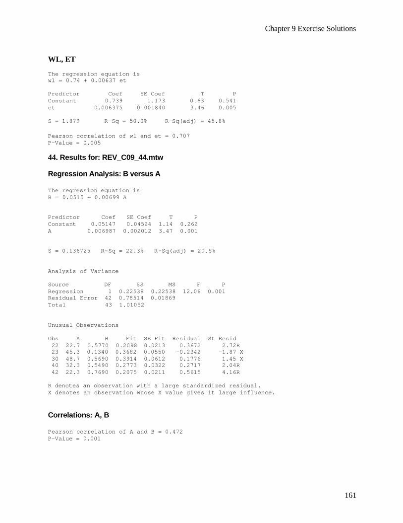
Chapter 9 Exercise Solutions
161
WL, ET The regression equation is wl = 0.74 + 0.00637 et Predictor Coef SE Coef T P Constant 0.739 1.173 0.63 0.541 et 0.006375 0.001840 3.46 0.005 S = 1.879 R-Sq = 50.0% R-Sq(adj) = 45.8% Pearson correlation of wl and et = 0.707 P-Value = 0.005 44. Results for: REV_C09_44.mtw Regression Analysis: B versus A The regression equation is B = 0.0515 + 0.00699 A Predictor Coef SE Coef T P Constant 0.05147 0.04524 1.14 0.262 A 0.006987 0.002012 3.47 0.001 S = 0.136725 R-Sq = 22.3% R-Sq(adj) = 20.5% Analysis of Variance Source DF SS MS F P Regression 1 0.22538 0.22538 12.06 0.001 Residual Error 42 0.78514 0.01869 Total 43 1.01052 Unusual Observations Obs A B Fit SE Fit Residual St Resid 22 22.7 0.5770 0.2098 0.0213 0.3672 2.72R 23 45.3 0.1340 0.3682 0.0550 -0.2342 -1.87 X 30 48.7 0.5690 0.3914 0.0612 0.1776 1.45 X 40 32.3 0.5490 0.2773 0.0322 0.2717 2.04R 42 22.3 0.7690 0.2075 0.0211 0.5615 4.16R R denotes an observation with a large standardized residual. X denotes an observation whose X value gives it large influence. Correlations: A, B Pearson correlation of A and B = 0.472 P-Value = 0.001
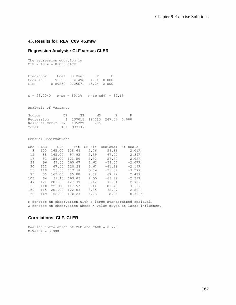
Chapter 9 Exercise Solutions
162
45. Results for: REV_C09_45.mtw Regression Analysis: CLF versus CLER The regression equation is CLF = 19.4 + 0.893 CLER Predictor Coef SE Coef T P Constant 19.393 4.496 4.31 0.000 CLER 0.89250 0.05671 15.74 0.000 S = 28.2040 R-Sq = 59.3% R-Sq(adj) = 59.1% Analysis of Variance Source DF SS MS F P Regression 1 197013 197013 247.67 0.000 Residual Error 170 135229 795 Total 171 332242 Unusual Observations Obs CLER CLF Fit SE Fit Residual St Resid 3 100 165.00 108.64 2.76 56.36 2.01R 15 88 165.00 97.93 2.39 67.07 2.39R 17 92 159.00 101.50 2.50 57.50 2.05R 28 96 47.00 105.07 2.62 -58.07 -2.07R 30 122 67.00 128.28 3.67 -61.28 -2.19R 53 110 26.00 117.57 3.14 -91.57 -3.27R 73 85 163.00 95.08 2.32 67.92 2.42R 103 94 39.10 103.02 2.55 -63.92 -2.28R 147 121 203.00 127.39 3.62 75.61 2.70R 155 110 221.00 117.57 3.14 103.43 3.69R 159 115 201.00 122.03 3.35 78.97 2.82R 162 169 162.00 170.23 6.03 -8.23 -0.30 X R denotes an observation with a large standardized residual. X denotes an observation whose X value gives it large influence. Correlations: CLF, CLER Pearson correlation of CLF and CLER = 0.770 P-Value = 0.000
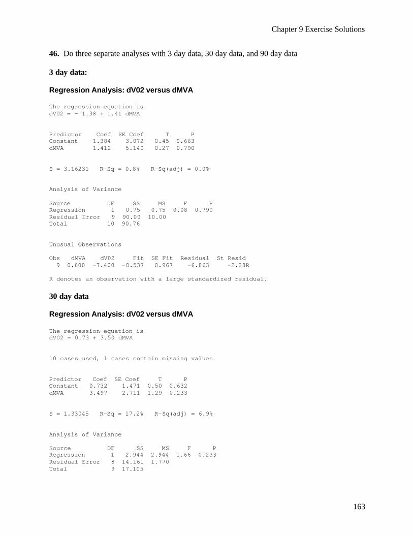
Chapter 9 Exercise Solutions
163
46. Do three separate analyses with 3 day data, 30 day data, and 90 day data 3 day data: Regression Analysis: dV02 versus dMVA The regression equation is dV02 = - 1.38 + 1.41 dMVA Predictor Coef SE Coef T P Constant -1.384 3.072 -0.45 0.663 dMVA 1.412 5.140 0.27 0.790 S = 3.16231 R-Sq = 0.8% R-Sq(adj) = 0.0% Analysis of Variance Source DF SS MS F P Regression 1 0.75 0.75 0.08 0.790 Residual Error 9 90.00 10.00 Total 10 90.76 Unusual Observations Obs dMVA dV02 Fit SE Fit Residual St Resid 9 0.600 -7.400 -0.537 0.967 -6.863 -2.28R R denotes an observation with a large standardized residual. 30 day data Regression Analysis: dV02 versus dMVA The regression equation is dV02 = 0.73 + 3.50 dMVA 10 cases used, 1 cases contain missing values Predictor Coef SE Coef T P Constant 0.732 1.471 0.50 0.632 dMVA 3.497 2.711 1.29 0.233 S = 1.33045 R-Sq = 17.2% R-Sq(adj) = 6.9% Analysis of Variance Source DF SS MS F P Regression 1 2.944 2.944 1.66 0.233 Residual Error 8 14.161 1.770 Total 9 17.105
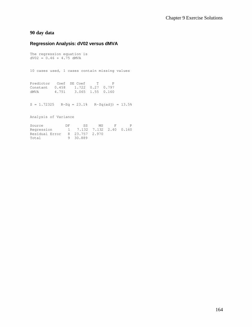
Chapter 9 Exercise Solutions
164
90 day data Regression Analysis: dV02 versus dMVA The regression equation is dV02 = 0.46 + 4.75 dMVA 10 cases used, 1 cases contain missing values Predictor Coef SE Coef T P Constant 0.458 1.722 0.27 0.797 dMVA 4.751 3.065 1.55 0.160 S = 1.72325 R-Sq = 23.1% R-Sq(adj) = 13.5% Analysis of Variance Source DF SS MS F P Regression 1 7.132 7.132 2.40 0.160 Residual Error 8 23.757 2.970 Total 9 30.889
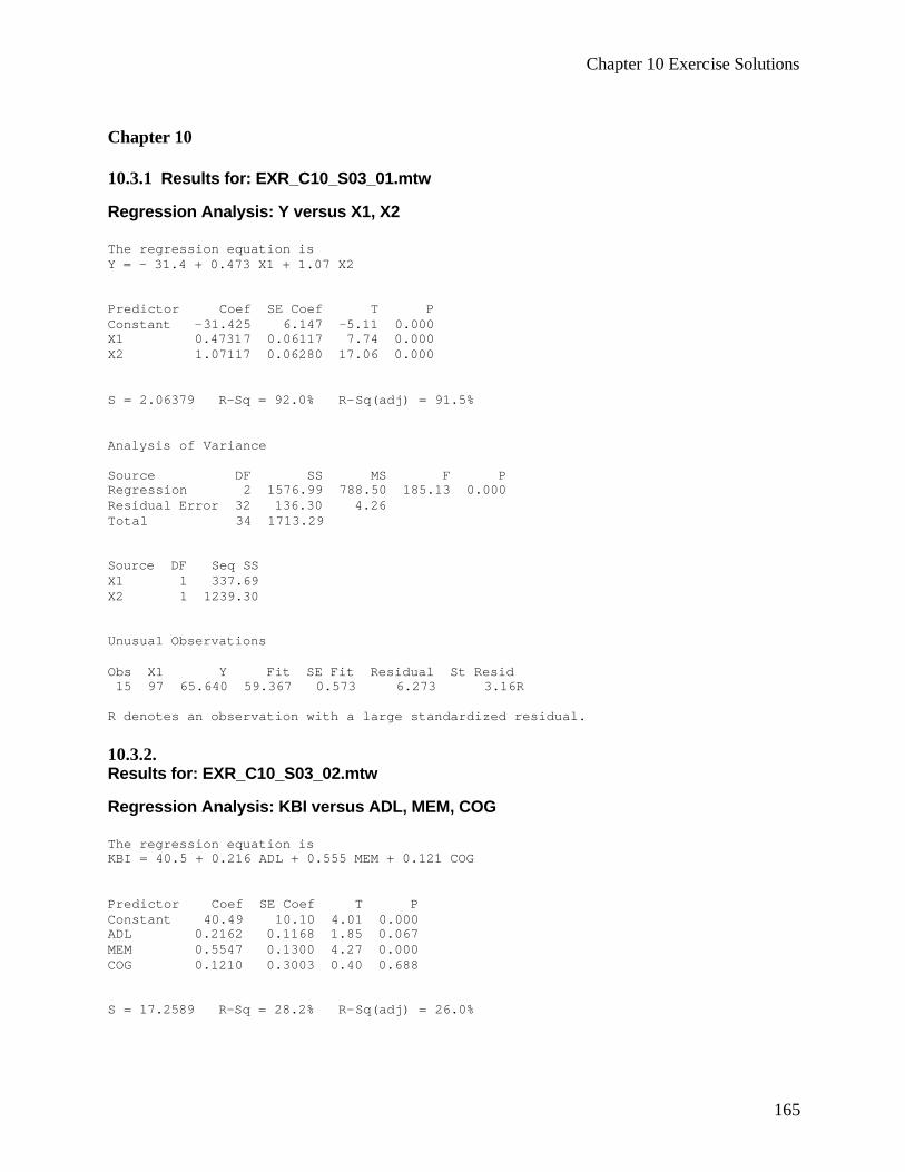
Chapter 10 Exercise Solutions
165
Chapter 10 10.3.1 Results for: EXR_C10_S03_01.mtw Regression Analysis: Y versus X1, X2 The regression equation is Y = - 31.4 + 0.473 X1 + 1.07 X2 Predictor Coef SE Coef T P Constant -31.425 6.147 -5.11 0.000 X1 0.47317 0.06117 7.74 0.000 X2 1.07117 0.06280 17.06 0.000 S = 2.06379 R-Sq = 92.0% R-Sq(adj) = 91.5% Analysis of Variance Source DF SS MS F P Regression 2 1576.99 788.50 185.13 0.000 Residual Error 32 136.30 4.26 Total 34 1713.29 Source DF Seq SS X1 1 337.69 X2 1 1239.30 Unusual Observations Obs X1 Y Fit SE Fit Residual St Resid 15 97 65.640 59.367 0.573 6.273 3.16R R denotes an observation with a large standardized residual. 10.3.2. Results for: EXR_C10_S03_02.mtw Regression Analysis: KBI versus ADL, MEM, COG The regression equation is KBI = 40.5 + 0.216 ADL + 0.555 MEM + 0.121 COG Predictor Coef SE Coef T P Constant 40.49 10.10 4.01 0.000 ADL 0.2162 0.1168 1.85 0.067 MEM 0.5547 0.1300 4.27 0.000 COG 0.1210 0.3003 0.40 0.688 S = 17.2589 R-Sq = 28.2% R-Sq(adj) = 26.0%
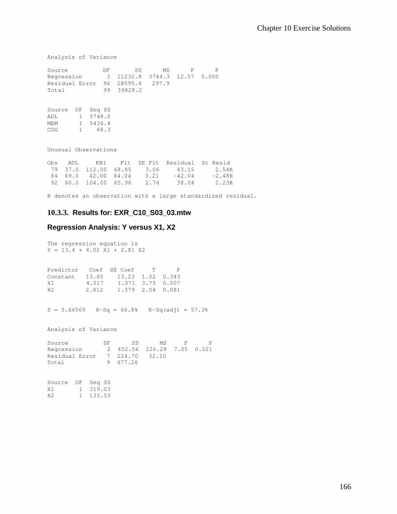
Chapter 10 Exercise Solutions
166
Analysis of Variance Source DF SS MS F P Regression 3 11232.8 3744.3 12.57 0.000 Residual Error 96 28595.4 297.9 Total 99 39828.2 Source DF Seq SS ADL 1 5748.0 MEM 1 5436.4 COG 1 48.3 Unusual Observations Obs ADL KBI Fit SE Fit Residual St Resid 79 37.0 112.00 68.85 3.06 43.15 2.54R 84 69.0 42.00 84.04 3.21 -42.04 -2.48R 92 60.0 104.00 65.96 2.76 38.04 2.23R R denotes an observation with a large standardized residual. 10.3.3. Results for: EXR_C10_S03_03.mtw Regression Analysis: Y versus X1, X2 The regression equation is Y = 13.4 + 4.02 X1 + 2.81 X2 Predictor Coef SE Coef T P Constant 13.45 13.23 1.02 0.343 X1 4.017 1.071 3.75 0.007 X2 2.812 1.379 2.04 0.081 S = 5.66569 R-Sq = 66.8% R-Sq(adj) = 57.3% Analysis of Variance Source DF SS MS F P Regression 2 452.56 226.28 7.05 0.021 Residual Error 7 224.70 32.10 Total 9 677.26 Source DF Seq SS X1 1 319.03 X2 1 133.53
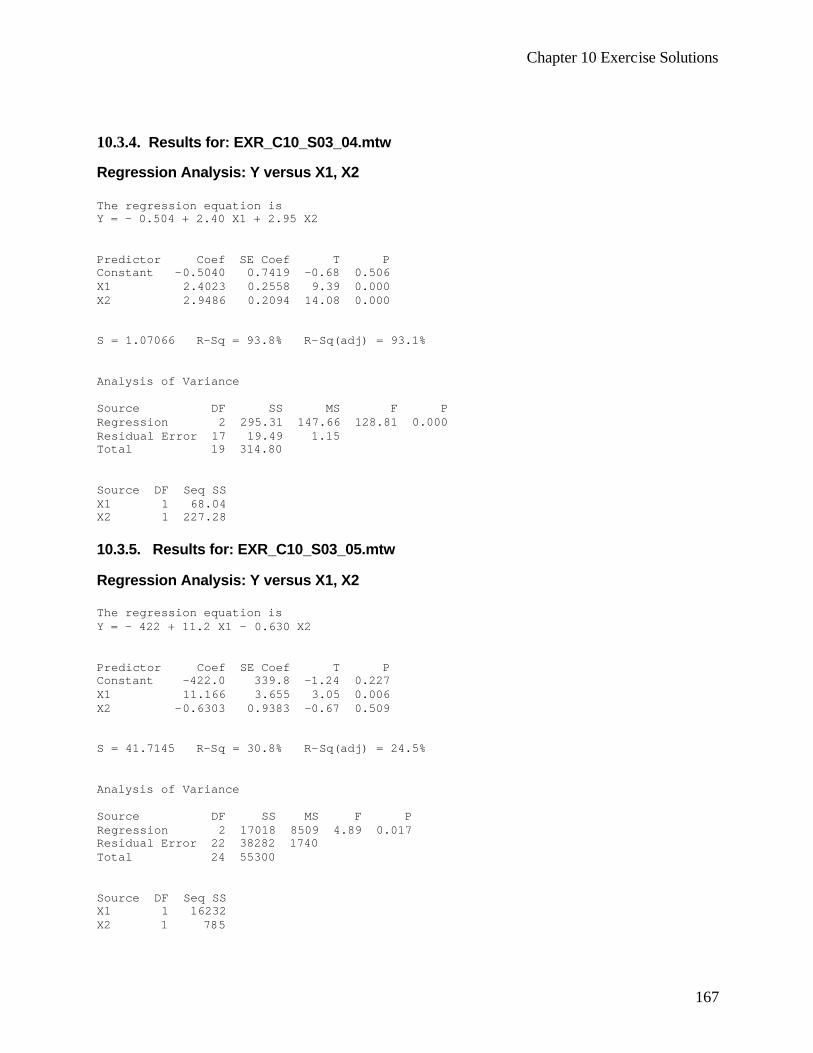
Chapter 10 Exercise Solutions
167
10.3.4. Results for: EXR_C10_S03_04.mtw Regression Analysis: Y versus X1, X2 The regression equation is Y = - 0.504 + 2.40 X1 + 2.95 X2 Predictor Coef SE Coef T P Constant -0.5040 0.7419 -0.68 0.506 X1 2.4023 0.2558 9.39 0.000 X2 2.9486 0.2094 14.08 0.000 S = 1.07066 R-Sq = 93.8% R-Sq(adj) = 93.1% Analysis of Variance Source DF SS MS F P Regression 2 295.31 147.66 128.81 0.000 Residual Error 17 19.49 1.15 Total 19 314.80 Source DF Seq SS X1 1 68.04 X2 1 227.28 10.3.5. Results for: EXR_C10_S03_05.mtw Regression Analysis: Y versus X1, X2 The regression equation is Y = - 422 + 11.2 X1 - 0.630 X2 Predictor Coef SE Coef T P Constant -422.0 339.8 -1.24 0.227 X1 11.166 3.655 3.05 0.006 X2 -0.6303 0.9383 -0.67 0.509 S = 41.7145 R-Sq = 30.8% R-Sq(adj) = 24.5% Analysis of Variance Source DF SS MS F P Regression 2 17018 8509 4.89 0.017 Residual Error 22 38282 1740 Total 24 55300 Source DF Seq SS X1 1 16232 X2 1 785
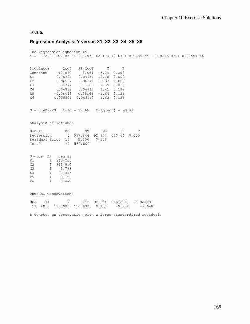
Chapter 10 Exercise Solutions
168
10.3.6. Regression Analysis: Y versus X1, X2, X3, X4, X5, X6 The regression equation is Y = - 12.9 + 0.703 X1 + 0.970 X2 + 3.78 X3 + 0.0684 X4 - 0.0845 X5 + 0.00557 X6 Predictor Coef SE Coef T P Constant -12.870 2.557 -5.03 0.000 X1 0.70326 0.04961 14.18 0.000 X2 0.96992 0.06311 15.37 0.000 X3 3.777 1.580 2.39 0.033 X4 0.06838 0.04844 1.41 0.182 X5 -0.08448 0.05161 -1.64 0.126 X6 0.005571 0.003412 1.63 0.126 S = 0.407229 R-Sq = 99.6% R-Sq(adj) = 99.4% Analysis of Variance Source DF SS MS F P Regression 6 557.844 92.974 560.64 0.000 Residual Error 13 2.156 0.166 Total 19 560.000 Source DF Seq SS X1 1 243.266 X2 1 311.910 X3 1 1.768 X4 1 0.335 X5 1 0.123 X6 1 0.442 Unusual Observations Obs X1 Y Fit SE Fit Residual St Resid 19 48.0 110.000 110.932 0.203 -0.932 -2.64R R denotes an observation with a large standardized residual.
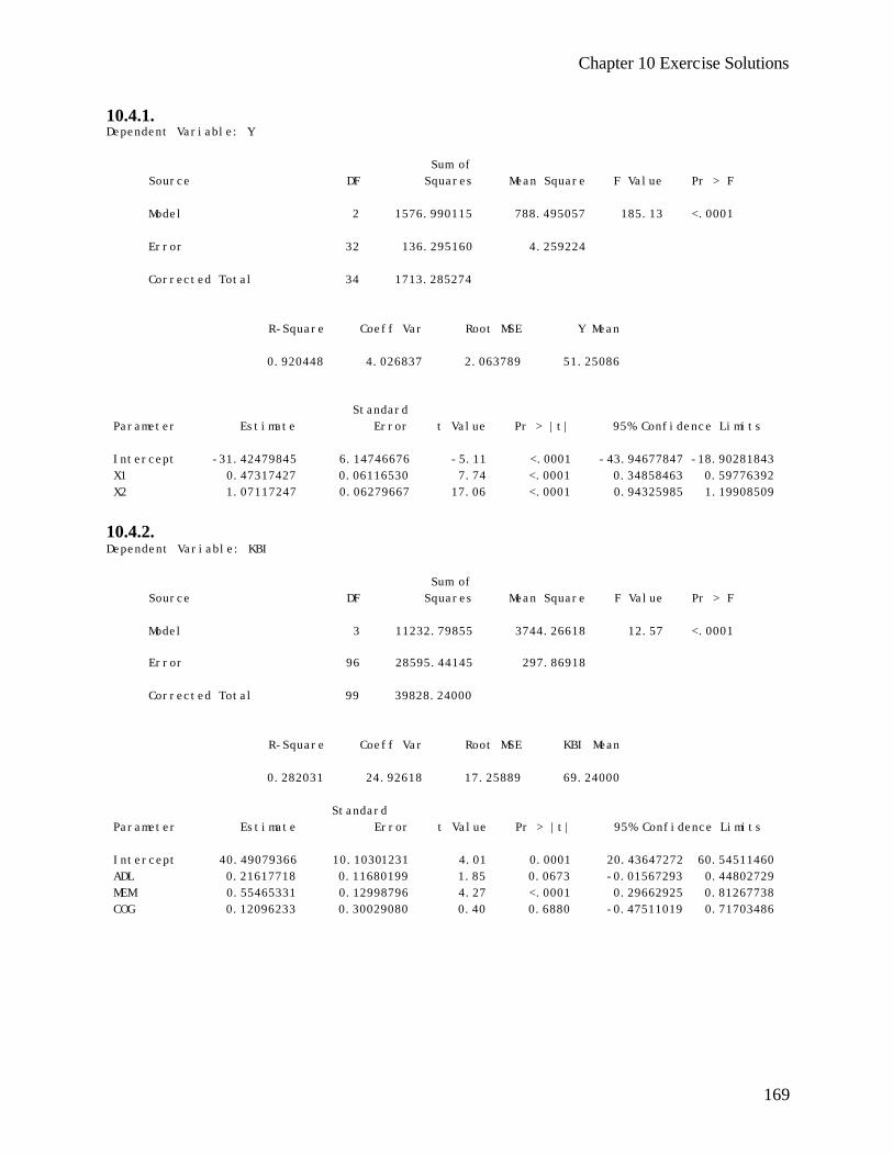
Chapter 10 Exercise Solutions
169
10.4.1. Dependent Variable: Y Sum of Source DF Squares Mean Square F Value Pr > F Model 2 1576.990115 788.495057 185.13 <.0001 Error 32 136.295160 4.259224 Corrected Total 34 1713.285274 R-Square Coeff Var Root MSE Y Mean 0.920448 4.026837 2.063789 51.25086 Standard Parameter Estimate Error t Value Pr > |t| 95% Confidence Limits Intercept -31.42479845 6.14746676 -5.11 <.0001 -43.94677847 -18.90281843 X1 0.47317427 0.06116530 7.74 <.0001 0.34858463 0.59776392 X2 1.07117247 0.06279667 17.06 <.0001 0.94325985 1.19908509 10.4.2. Dependent Variable: KBI Sum of Source DF Squares Mean Square F Value Pr > F Model 3 11232.79855 3744.26618 12.57 <.0001 Error 96 28595.44145 297.86918 Corrected Total 99 39828.24000 R-Square Coeff Var Root MSE KBI Mean 0.282031 24.92618 17.25889 69.24000 Standard Parameter Estimate Error t Value Pr > |t| 95% Confidence Limits Intercept 40.49079366 10.10301231 4.01 0.0001 20.43647272 60.54511460 ADL 0.21617718 0.11680199 1.85 0.0673 -0.01567293 0.44802729 MEM 0.55465331 0.12998796 4.27 <.0001 0.29662925 0.81267738 COG 0.12096233 0.30029080 0.40 0.6880 -0.47511019 0.71703486
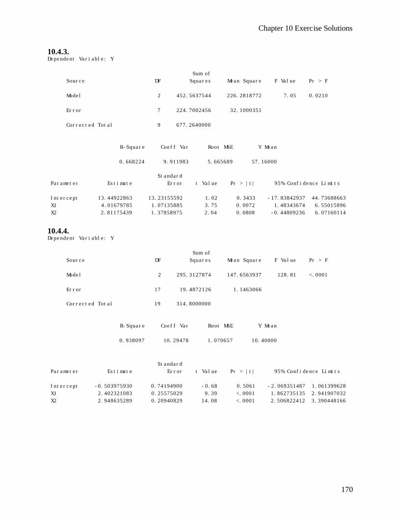
Chapter 10 Exercise Solutions
170
10.4.3. Dependent Variable: Y Sum of Source DF Squares Mean Square F Value Pr > F Model 2 452.5637544 226.2818772 7.05 0.0210 Error 7 224.7002456 32.1000351 Corrected Total 9 677.2640000 R-Square Coeff Var Root MSE Y Mean 0.668224 9.911983 5.665689 57.16000 Standard Parameter Estimate Error t Value Pr > |t| 95% Confidence Limits Intercept 13.44922863 13.23155592 1.02 0.3433 -17.83842937 44.73688663 X1 4.01679785 1.07135885 3.75 0.0072 1.48343674 6.55015896 X2 2.81175439 1.37858975 2.04 0.0808 -0.44809236 6.07160114 10.4.4. Dependent Variable: Y Sum of Source DF Squares Mean Square F Value Pr > F Model 2 295.3127874 147.6563937 128.81 <.0001 Error 17 19.4872126 1.1463066 Corrected Total 19 314.8000000 R-Square Coeff Var Root MSE Y Mean 0.938097 10.29478 1.070657 10.40000 Standard Parameter Estimate Error t Value Pr > |t| 95% Confidence Limits Intercept -0.503975930 0.74194900 -0.68 0.5061 -2.069351487 1.061399628 X1 2.402321083 0.25575029 9.39 <.0001 1.862735135 2.941907032 X2 2.948635289 0.20940829 14.08 <.0001 2.506822412 3.390448166

Chapter 10 Exercise Solutions
171
10.4.5. Dependent Variable: Y Sum of Source DF Squares Mean Square F Value Pr > F Model 2 17017.78484 8508.89242 4.89 0.0175 Error 22 38282.21516 1740.10069 Corrected Total 24 55300.00000 R-Square Coeff Var Root MSE Y Mean 0.307736 7.768066 41.71451 537.0000 Standard Parameter Estimate Error t Value Pr > |t| 95% Confidence Limits Intercept -421.9967138 339.7619898 -1.24 0.2273 -1126.619954 282.6265263 X1 11.1661344 3.6552338 3.05 0.0058 3.5856435 18.7466253 X2 -0.6303187 0.9382608 -0.67 0.5087 -2.5761524 1.3155151 10.4.6. Dependent Variable: Y Sum of Source DF Squares Mean Square F Value Pr > F Model 6 557.8441423 92.9740237 560.64 <.0001 Error 13 2.1558577 0.1658352 Corrected Total 19 560.0000000 R-Square Coeff Var Root MSE Y Mean 0.996150 0.357218 0.407229 114.000 Standard Parameter Estimate Error t Value Pr > |t| 95% Confidence Limits Intercept -12.87047602 2.55664988 -5.03 0.0002 -18.39378229 -7.34716976 X1 0.70325939 0.04960581 14.18 <.0001 0.59609257 0.81042622 X2 0.96991978 0.06310846 15.37 <.0001 0.83358225 1.10625731 X3 3.77649100 1.58015087 2.39 0.0327 0.36278260 7.19019941 X4 0.06838304 0.04844149 1.41 0.1815 -0.03626844 0.17303452 X5 -0.08448469 0.05160898 -1.64 0.1256 -0.19597911 0.02700974 X6 0.00557150 0.00341230 1.63 0.1265 -0.00180033 0.01294333

Chapter 10 Exercise Solutions
172
10.5.1. CI: 50.289, 51.747 PI: 46.751, 55.284 10.5.2. CI: 59.82,70.29 PI: 30.40, 99.71 10.5.3. CI: 44.22, 56.59 PI: 35.64, 65.17 10.5.4. CI: 7.09, 8.51 PI: 5.43, 10.16 10.5.5. CI: 514.31, 550.75 PI: 444.12, 620.94 10.5.6. CI: 116.017,116.887 PI: 115.470, 117.433 10.6.1. (a) Pairwise correlations: Correlations: Y, X1, X2, X3 Y X1 X2 X1 0.360 0.022 X2 0.532 0.303 0.000 0.058 X3 0.202 0.674 0.430 0.211 0.000 0.006 Cell Contents: Pearson correlation P-Value
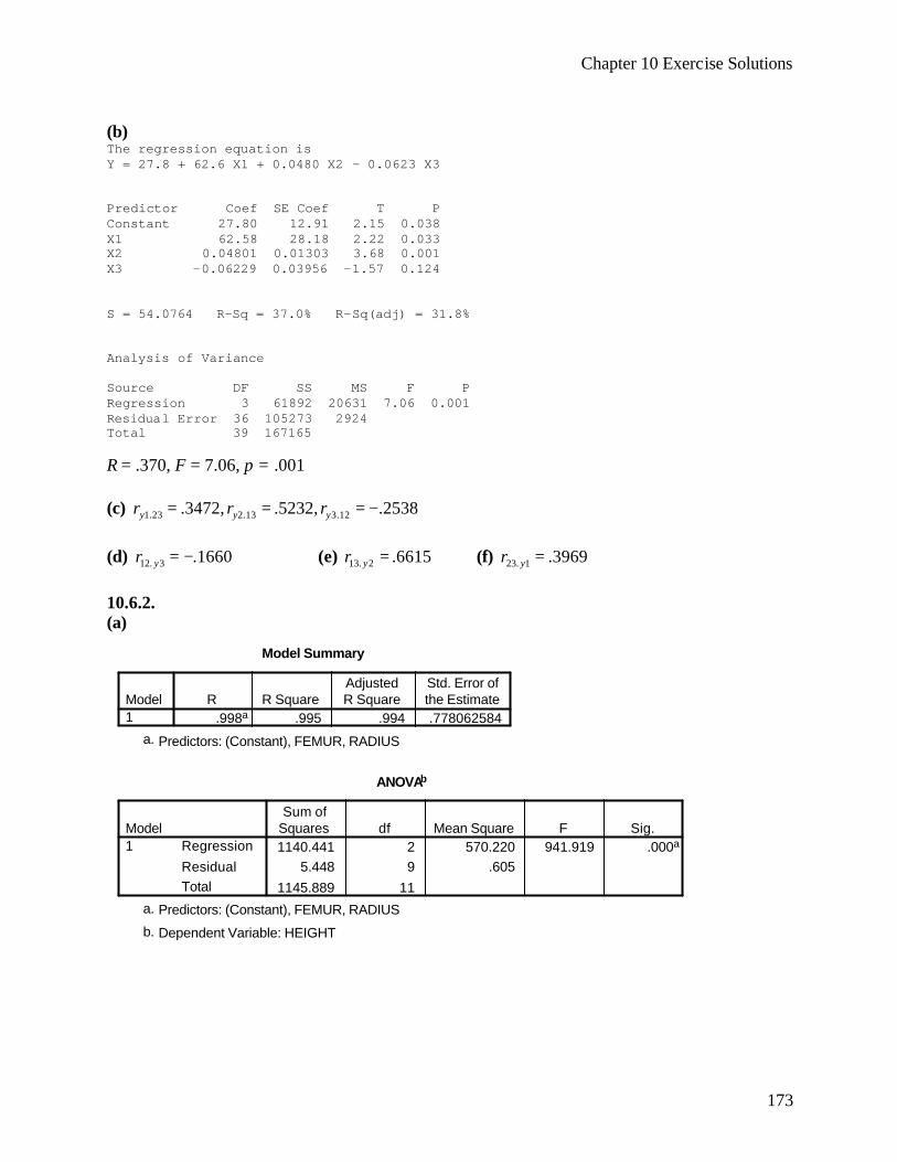
Chapter 10 Exercise Solutions
173
(b) The regression equation is Y = 27.8 + 62.6 X1 + 0.0480 X2 - 0.0623 X3 Predictor Coef SE Coef T P Constant 27.80 12.91 2.15 0.038 X1 62.58 28.18 2.22 0.033 X2 0.04801 0.01303 3.68 0.001 X3 -0.06229 0.03956 -1.57 0.124 S = 54.0764 R-Sq = 37.0% R-Sq(adj) = 31.8% Analysis of Variance Source DF SS MS F P Regression 3 61892 20631 7.06 0.001 Residual Error 36 105273 2924 Total 39 167165 R = .370, F = 7.06, p = .001 (c) 1.23 2.13 3.12.3472, .5232, .2538y y yr r r= = = − (d) 12. 3 .1660yr = − (e) 13. 2 .6615yr = (f) 23. 1 .3969yr = 10.6.2. (a)
Model Summary
.998a .995 .994 .778062584Model1
R R SquareAdjustedR Square
Std. Error ofthe Estimate
Predictors: (Constant), FEMUR, RADIUSa.
ANOVAb
1140.441 2 570.220 941.919 .000a
5.448 9 .605
1145.889 11
Regression
ResidualTotal
Model1
Sum ofSquares df Mean Square F Sig.
Predictors: (Constant), FEMUR, RADIUSa.
Dependent Variable: HEIGHTb.
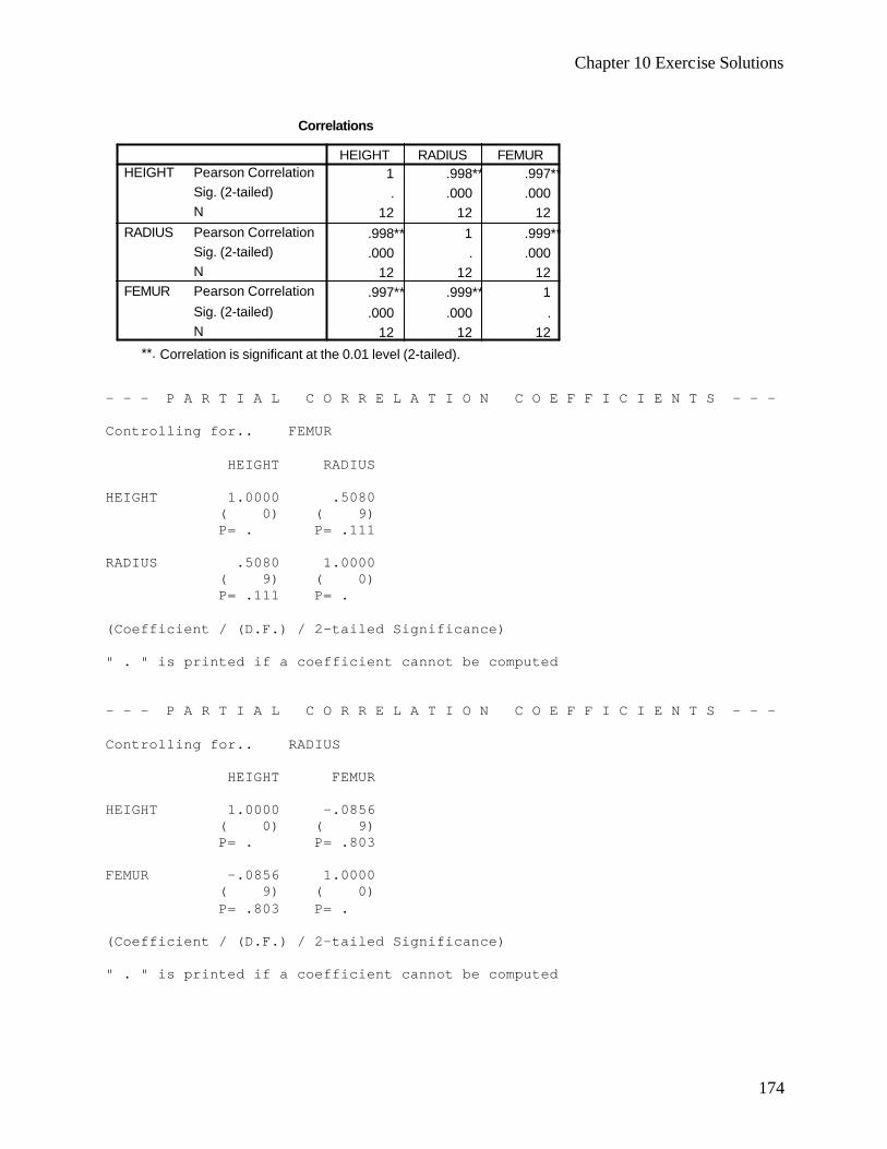
Chapter 10 Exercise Solutions
174
Correlations
1 .998** .997**. .000 .000
12 12 12
.998** 1 .999**
.000 . .00012 12 12
.997** .999** 1
.000 .000 .12 12 12
Pearson CorrelationSig. (2-tailed)N
Pearson CorrelationSig. (2-tailed)NPearson Correlation
Sig. (2-tailed)N
HEIGHT
RADIUS
FEMUR
HEIGHT RADIUS FEMUR
Correlation is significant at the 0.01 level (2-tailed).**.
- - - P A R T I A L C O R R E L A T I O N C O E F F I C I E N T S - - - Controlling for.. FEMUR HEIGHT RADIUS HEIGHT 1.0000 .5080 ( 0) ( 9) P= . P= .111 RADIUS .5080 1.0000 ( 9) ( 0) P= .111 P= . (Coefficient / (D.F.) / 2-tailed Significance) " . " is printed if a coefficient cannot be computed - - - P A R T I A L C O R R E L A T I O N C O E F F I C I E N T S - - - Controlling for.. RADIUS HEIGHT FEMUR HEIGHT 1.0000 -.0856 ( 0) ( 9) P= . P= .803 FEMUR -.0856 1.0000 ( 9) ( 0) P= .803 P= . (Coefficient / (D.F.) / 2-tailed Significance) " . " is printed if a coefficient cannot be computed
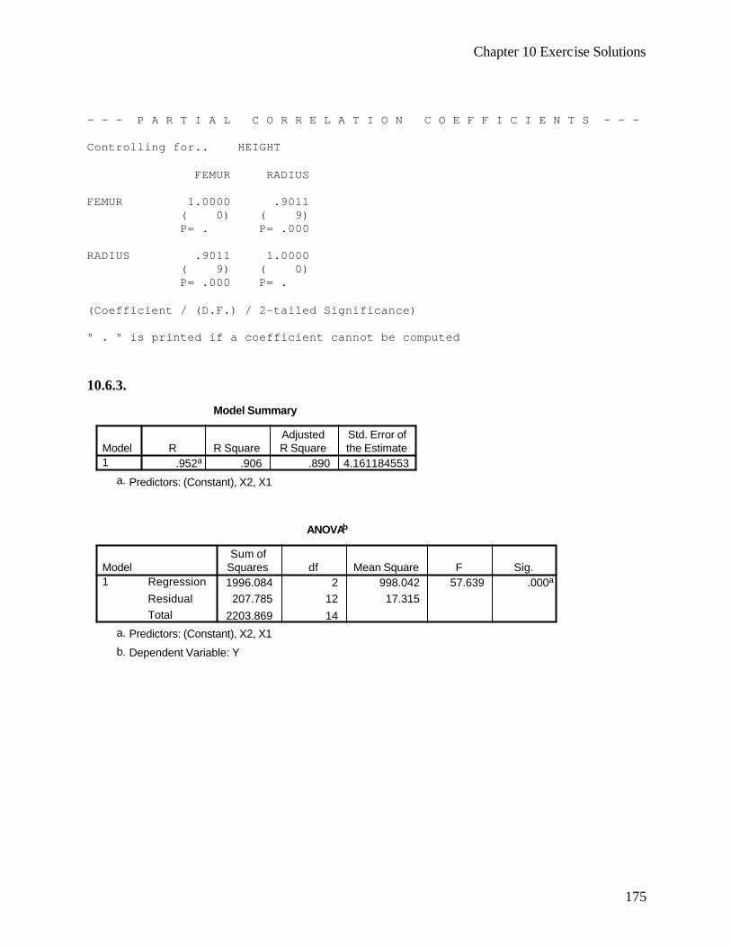
Chapter 10 Exercise Solutions
175
- - - P A R T I A L C O R R E L A T I O N C O E F F I C I E N T S - - - Controlling for.. HEIGHT FEMUR RADIUS FEMUR 1.0000 .9011 ( 0) ( 9) P= . P= .000 RADIUS .9011 1.0000 ( 9) ( 0) P= .000 P= . (Coefficient / (D.F.) / 2-tailed Significance) " . " is printed if a coefficient cannot be computed 10.6.3.
Model Summary
.952a .906 .890 4.161184553Model1
R R SquareAdjustedR Square
Std. Error ofthe Estimate
Predictors: (Constant), X2, X1a.
ANOVAb
1996.084 2 998.042 57.639 .000a
207.785 12 17.315
2203.869 14
Regression
ResidualTotal
Model1
Sum ofSquares df Mean Square F Sig.
Predictors: (Constant), X2, X1a.
Dependent Variable: Yb.
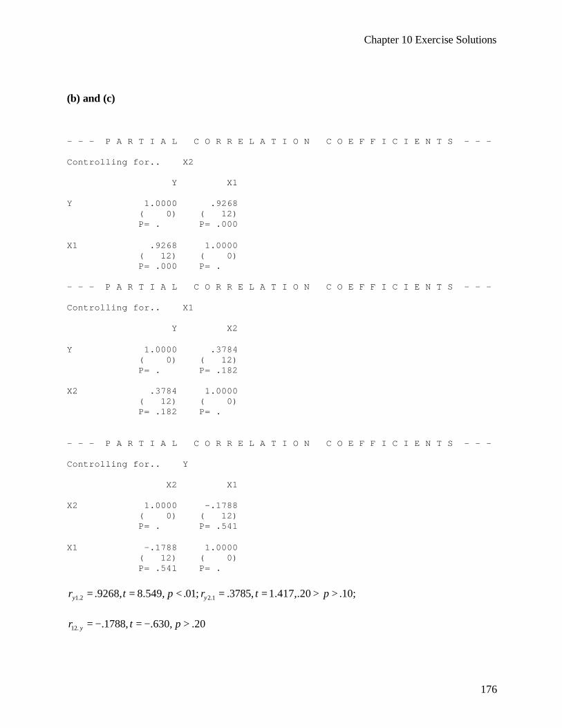
Chapter 10 Exercise Solutions
176
(b) and (c) - - - P A R T I A L C O R R E L A T I O N C O E F F I C I E N T S - - - Controlling for.. X2 Y X1 Y 1.0000 .9268 ( 0) ( 12) P= . P= .000 X1 .9268 1.0000 ( 12) ( 0) P= .000 P= . - - - P A R T I A L C O R R E L A T I O N C O E F F I C I E N T S - - - Controlling for.. X1 Y X2 Y 1.0000 .3784 ( 0) ( 12) P= . P= .182 X2 .3784 1.0000 ( 12) ( 0) P= .182 P= . - - - P A R T I A L C O R R E L A T I O N C O E F F I C I E N T S - - - Controlling for.. Y X2 X1 X2 1.0000 -.1788 ( 0) ( 12) P= . P= .541 X1 -.1788 1.0000 ( 12) ( 0) P= .541 P= .
1.2 2.1.9268, 8.549, .01; .3785, 1.417,.20 .10;y yr t p r t p= = < = = > >
12. .1788, .630, .20yr t p= − = − >
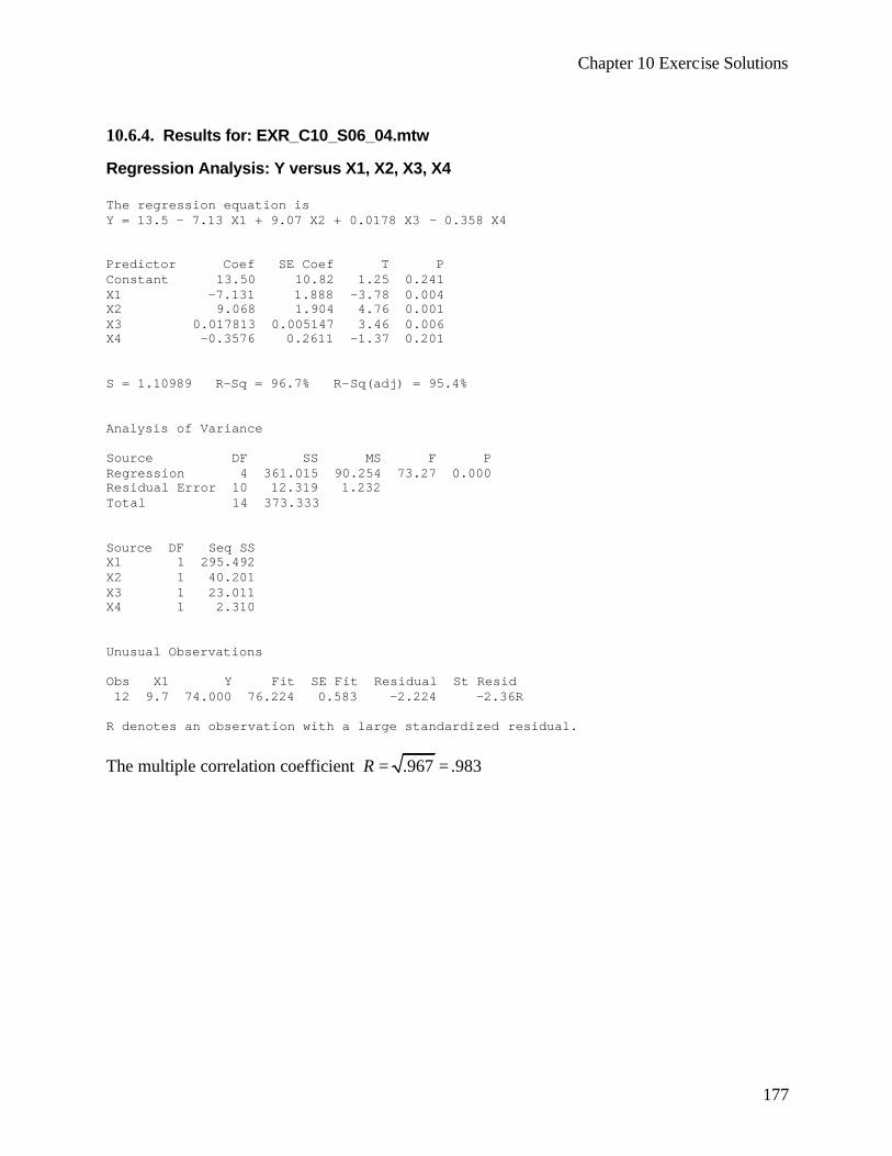
Chapter 10 Exercise Solutions
177
10.6.4. Results for: EXR_C10_S06_04.mtw Regression Analysis: Y versus X1, X2, X3, X4 The regression equation is Y = 13.5 - 7.13 X1 + 9.07 X2 + 0.0178 X3 - 0.358 X4 Predictor Coef SE Coef T P Constant 13.50 10.82 1.25 0.241 X1 -7.131 1.888 -3.78 0.004 X2 9.068 1.904 4.76 0.001 X3 0.017813 0.005147 3.46 0.006 X4 -0.3576 0.2611 -1.37 0.201 S = 1.10989 R-Sq = 96.7% R-Sq(adj) = 95.4% Analysis of Variance Source DF SS MS F P Regression 4 361.015 90.254 73.27 0.000 Residual Error 10 12.319 1.232 Total 14 373.333 Source DF Seq SS X1 1 295.492 X2 1 40.201 X3 1 23.011 X4 1 2.310 Unusual Observations Obs X1 Y Fit SE Fit Residual St Resid 12 9.7 74.000 76.224 0.583 -2.224 -2.36R R denotes an observation with a large standardized residual.
The multiple correlation coefficient .967 .983R = =
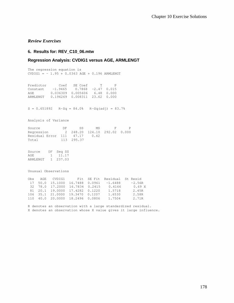
Chapter 10 Exercise Solutions
178
Review Exercises 6. Results for: REV_C10_06.mtw Regression Analysis: CVDIG1 versus AGE, ARMLENGT The regression equation is CVDIG1 = - 1.95 + 0.0363 AGE + 0.196 ARMLENGT Predictor Coef SE Coef T P Constant -1.9465 0.7868 -2.47 0.015 AGE 0.036309 0.005606 6.48 0.000 ARMLENGT 0.196269 0.008311 23.62 0.000 S = 0.651892 R-Sq = 84.0% R-Sq(adj) = 83.7% Analysis of Variance Source DF SS MS F P Regression 2 248.20 124.10 292.02 0.000 Residual Error 111 47.17 0.42 Total 113 295.37 Source DF Seq SS AGE 1 11.17 ARMLENGT 1 237.03 Unusual Observations Obs AGE CVDIG1 Fit SE Fit Residual St Resid 17 50.0 15.1000 16.7488 0.0961 -1.6488 -2.56R 32 78.0 17.2000 16.7834 0.2415 0.4166 0.69 X 81 20.1 19.0000 17.4282 0.1220 1.5718 2.45R 106 35.1 21.0000 19.3470 0.1207 1.6530 2.58R 110 40.0 20.0000 18.2496 0.0806 1.7504 2.71R R denotes an observation with a large standardized residual. X denotes an observation whose X value gives it large influence.
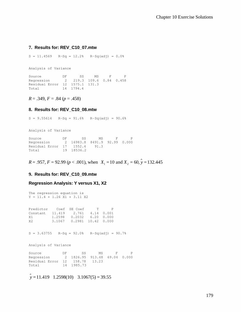
Chapter 10 Exercise Solutions
179
7. Results for: REV_C10_07.mtw S = 11.4569 R-Sq = 12.2% R-Sq(adj) = 0.0% Analysis of Variance Source DF SS MS F P Regression 2 219.3 109.6 0.84 0.458 Residual Error 12 1575.1 131.3 Total 14 1794.4 R = .349, F = .84 (p = .458) 8. Results for: REV_C10_08.mtw S = 9.55614 R-Sq = 91.6% R-Sq(adj) = 90.6% Analysis of Variance Source DF SS MS F P Regression 2 16983.8 8491.9 92.99 0.000 Residual Error 17 1552.4 91.3 Total 19 18536.2 R = .957, F = 92.99 (p < .001), when $
1 210 and 60, 132.445X X y= = = 9. Results for: REV_C10_09.mtw Regression Analysis: Y versus X1, X2 The regression equation is Y = 11.4 + 1.26 X1 + 3.11 X2 Predictor Coef SE Coef T P Constant 11.419 2.761 4.14 0.001 X1 1.2598 0.2032 6.20 0.000 X2 3.1067 0.2981 10.42 0.000 S = 3.63755 R-Sq = 92.0% R-Sq(adj) = 90.7% Analysis of Variance Source DF SS MS F P Regression 2 1826.95 913.48 69.04 0.000 Residual Error 12 158.78 13.23 Total 14 1985.73 $ 11.419 1.2598(10) 3.1067(5) 39.55y = + + =
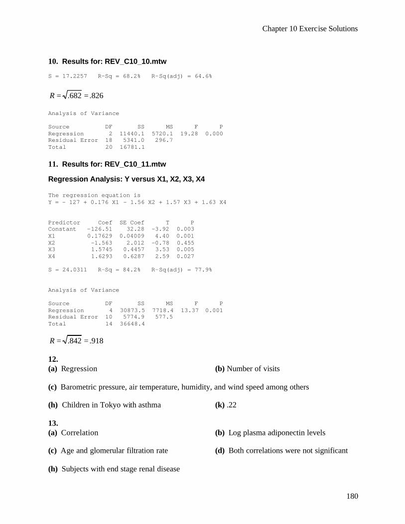
Chapter 10 Exercise Solutions
180
10. Results for: REV_C10_10.mtw S = 17.2257 R-Sq = 68.2% R-Sq(adj) = 64.6%
.682 .826R = = Analysis of Variance Source DF SS MS F P Regression 2 11440.1 5720.1 19.28 0.000 Residual Error 18 5341.0 296.7 Total 20 16781.1 11. Results for: REV_C10_11.mtw Regression Analysis: Y versus X1, X2, X3, X4 The regression equation is Y = - 127 + 0.176 X1 - 1.56 X2 + 1.57 X3 + 1.63 X4 Predictor Coef SE Coef T P Constant -126.51 32.28 -3.92 0.003 X1 0.17629 0.04009 4.40 0.001 X2 -1.563 2.012 -0.78 0.455 X3 1.5745 0.4457 3.53 0.005 X4 1.6293 0.6287 2.59 0.027 S = 24.0311 R-Sq = 84.2% R-Sq(adj) = 77.9% Analysis of Variance Source DF SS MS F P Regression 4 30873.5 7718.4 13.37 0.001 Residual Error 10 5774.9 577.5 Total 14 36648.4
.842 .918R = = 12. (a) Regression (b) Number of visits (c) Barometric pressure, air temperature, humidity, and wind speed among others (h) Children in Tokyo with asthma (k) .22 13. (a) Correlation (b) Log plasma adiponectin levels (c) Age and glomerular filtration rate (d) Both correlations were not significant (h) Subjects with end stage renal disease
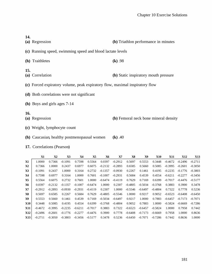
Chapter 10 Exercise Solutions
181
14. (a) Regression (b) Triathlon performance in minutes (c) Running speed, swimming speed and blood lactate levels (h) Traithletes (k) .98 15. (a) Correlation (b) Static inspiratory mouth pressure (c) Forced expiratory volume, peak expiratory flow, maximal inspiratory flow (d) Both correlations were not significant (h) Boys and girls ages 7-14 16. (a) Regression (b) Femoral neck bone mineral density (c) Weight, lymphocyte count (h) Caucasian, healthy postmenopausal women (k) .40 17. Correlations (Pearson) X1 X2 X3 X4 X5 X6 X7 X8 X9 X10 X11 X12 X13
X1 1.0000 0.7366 -0.1091 0.7598 0.5564 0.0397 -0.2912 0.5697 0.5553 0.3448 -0.4672 -0.2496 -0.2711 X2 0.7366 1.0000 0.2437 0.6977 0.6075 -0.2132 -0.2893 0.6585 0.5660 0.5085 -0.3995 -0.2601 -0.3050 X3 -0.1091 0.2437 1.0000 0.3164 0.2732 -0.1357 -0.0930 0.2267 0.1461 0.4195 -0.2235 -0.1776 -0.3803 X4 0.7598 0.6977 0.3164 1.0000 0.7601 -0.1007 -0.2931 0.5684 0.4539 0.4554 -0.6211 -0.2277 -0.3456 X5 0.5564 0.6075 0.2732 0.7601 1.0000 -0.6474 -0.4119 0.7629 0.7169 0.6399 -0.7017 -0.4476 -0.5177 X6 0.0397 -0.2132 -0.1357 -0.1007 -0.6474 1.0000 0.2307 -0.4805 -0.5034 -0.3768 0.3883 0.3900 0.3478 X7 -0.2912 -0.2893 -0.0930 -0.2931 -0.4119 0.2307 1.0000 -0.5546 -0.6497 -0.4804 0.7322 0.7778 0.5236 X8 0.5697 0.6585 0.2267 0.5684 0.7629 -0.4805 -0.5546 1.0000 0.9217 0.9052 -0.6523 -0.6408 -0.6450 X9 0.5553 0.5660 0.1461 0.4539 0.7169 -0.5034 -0.6497 0.9217 1.0000 0.7883 -0.6457 -0.7173 -0.7071 X10 0.3448 0.5085 0.4195 0.4554 0.6399 -0.3768 -0.4804 0.9052 0.7883 1.0000 -0.5824 -0.6669 -0.7286 X11 -0.4672 -0.3995 -0.2235 -0.6211 -0.7017 0.3883 0.7322 -0.6523 -0.6457 -0.5824 1.0000 0.7958 0.7442 X12 -0.2496 -0.2601 -0.1776 -0.2277 -0.4476 0.3900 0.7778 -0.6408 -0.7173 -0.6669 0.7958 1.0000 0.8636 X13 -0.2711 -0.3050 -0.3803 -0.3456 -0.5177 0.3478 0.5236 -0.6450 -0.7071 -0.7286 0.7442 0.8636 1.0000

Chapter 10 Exercise Solutions
182
18. Results for: REV_C10_18.mtw(DISEASE = 1.000000) Correlations: C1, C2, C3, C4, C5, C6 C1 C2 C3 C4 C5 C2 0.989 C3 -0.187 -0.323 C4 -0.636 -0.606 -0.093 C5 0.554 0.580 -0.393 -0.466 C6 0.693 0.727 -0.434 -0.509 0.918 Cell Contents: Pearson correlation Results for: REV_C10_18.mtw(DISEASE = 2.000000) Correlations: C1, C4, C5, C6 C1 C4 C5 C4 -0.822 C5 -0.034 0.120 C6 -0.171 0.249 0.906 Cell Contents: Pearson correlation 19. Results for: REV_C10_19.mtw Correlations: C1, C2, C3, C4, C5, C6, C7, C8 C1 C2 C3 C4 C5 C6 C7 C2 0.123 C3 0.115 0.963 C4 0.417 -0.063 -0.041 C5 0.005 -0.102 -0.103 -0.059 C6 0.001 0.270 0.295 -0.036 0.137 C7 -0.113 -0.074 -0.076 0.052 0.134 0.061 C8 0.077 -0.002 -0.023 0.146 0.165 -0.202 -0.032
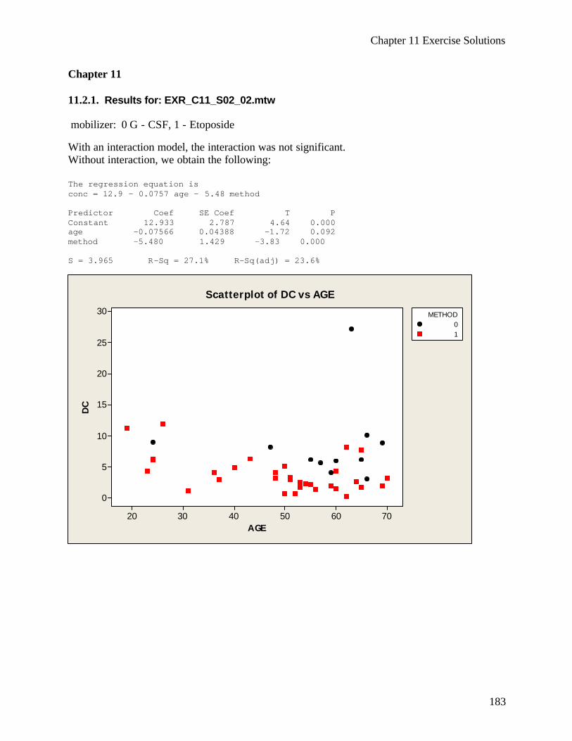
Chapter 11 Exercise Solutions
183
Chapter 11 11.2.1. Results for: EXR_C11_S02_02.mtw mobilizer: 0 G - CSF, 1 - Etoposide With an interaction model, the interaction was not significant. Without interaction, we obtain the following: The regression equation is conc = 12.9 - 0.0757 age - 5.48 method Predictor Coef SE Coef T P Constant 12.933 2.787 4.64 0.000 age -0.07566 0.04388 -1.72 0.092 method -5.480 1.429 -3.83 0.000 S = 3.965 R-Sq = 27.1% R-Sq(adj) = 23.6%
AGE
DC
706050403020
30
25
20
15
10
5
0
METHOD01
Scatterplot of DC vs AGE
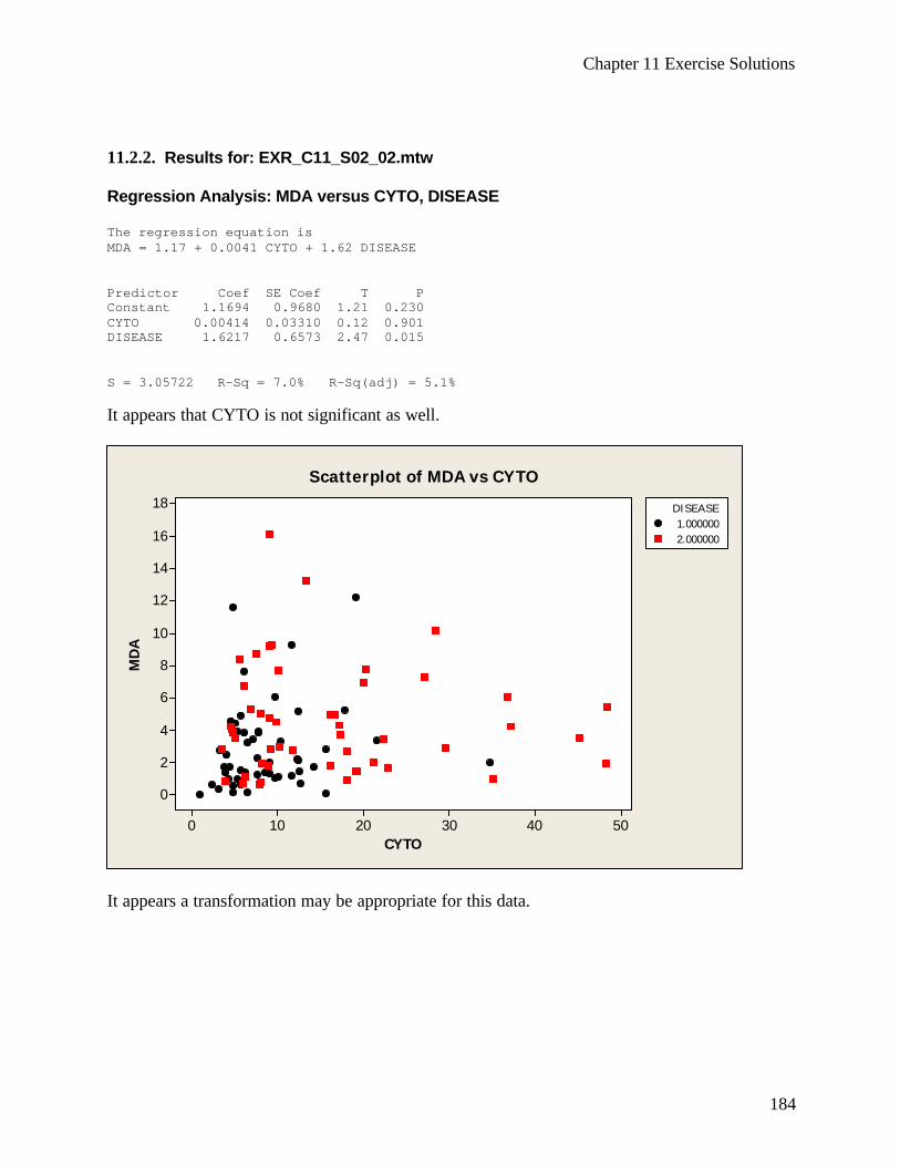
Chapter 11 Exercise Solutions
184
11.2.2. Results for: EXR_C11_S02_02.mtw Regression Analysis: MDA versus CYTO, DISEASE The regression equation is MDA = 1.17 + 0.0041 CYTO + 1.62 DISEASE Predictor Coef SE Coef T P Constant 1.1694 0.9680 1.21 0.230 CYTO 0.00414 0.03310 0.12 0.901 DISEASE 1.6217 0.6573 2.47 0.015 S = 3.05722 R-Sq = 7.0% R-Sq(adj) = 5.1% It appears that CYTO is not significant as well.
CYTO
MD
A
50403020100
18
16
14
12
10
8
6
4
2
0
DISEASE1.0000002.000000
Scatterplot of MDA vs CYTO
It appears a transformation may be appropriate for this data.
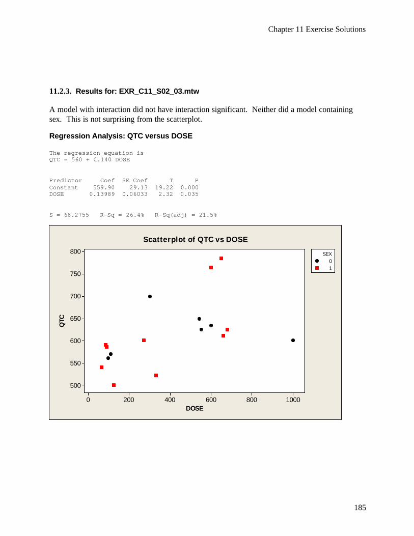
Chapter 11 Exercise Solutions
185
11.2.3. Results for: EXR_C11_S02_03.mtw A model with interaction did not have interaction significant. Neither did a model containing sex. This is not surprising from the scatterplot. Regression Analysis: QTC versus DOSE The regression equation is QTC = 560 + 0.140 DOSE Predictor Coef SE Coef T P Constant 559.90 29.13 19.22 0.000 DOSE 0.13989 0.06033 2.32 0.035 S = 68.2755 R-Sq = 26.4% R-Sq(adj) = 21.5%
DOSE
QTC
10008006004002000
800
750
700
650
600
550
500
SEX01
Scatterplot of QTC vs DOSE
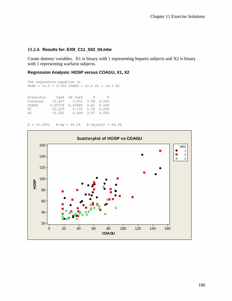
Chapter 11 Exercise Solutions
186
11.2.4. Results for: EXR_C11_S02_04.mtw Create dummy variables. X1 is binary with 1 representing heparin subjects and X2 is binary with 1 representing warfarin subjects. Regression Analysis: HOSP versus COAGU, X1, X2 The regression equation is HOSP = 15.5 + 0.558 COAGU + 22.2 X1 + 16.3 X2 Predictor Coef SE Coef T P Constant 15.457 3.871 3.99 0.000 COAGU 0.55758 0.05685 9.81 0.000 X1 22.229 4.135 5.38 0.000 X2 16.252 4.090 3.97 0.000 S = 15.4951 R-Sq = 66.1% R-Sq(adj) = 64.9%
COAGU
HO
SP
160140120100806040200
160
140
120
100
80
60
40
20
MED123
Scatterplot of HOSP vs COAGU
Chapter 11 Exercise Solutions
187
11.3.1. Results for: EXR_C11_S03_01.mtw Stepwise Regression: MMO versus AGE, DOWNCON, ... Forward selection. Alpha-to-Enter: 0.25 Step 1 2 3 Constant 51.93 116.07 115.54 MEM 0.66 0.60 0.57 T-Value 5.75 5.87 5.53 P-Value 0.000 0.000 0.000 SOCIALSU -0.476 -0.492 T-Value -5.28 -5.51 P-Value 0.000 0.000 CGDUR 0.122 T-Value 1.88 P-Value 0.064 S 17.4 15.4 15.2 R-Sq 25.20 41.92 43.97 R-Sq(adj) 24.44 40.72 42.22 It would be up to the investigator to include CGDUR in the model since its p value is very close to .05. MINITAB identifies variables with p values at .25 or less.

Chapter 11 Exercise Solutions
188
11.3.2. Results for: EXR_C11_S03_02.mtw Stepwise Regression: MMO versus AGE, DOWNCON, ... Forward selection. Alpha-to-Enter: 0.25 Response is MMO on 6 predictors, with N = 35 Step 1 2 3 Constant 31.515 -10.663 7.328 FROWCON 1.08 0.98 0.79 T-Value 4.00 3.98 2.93 P-Value 0.000 0.000 0.006 MANLENG 0.46 0.57 T-Value 2.85 3.31 P-Value 0.008 0.002 MANWIDT -0.21 T-Value -1.58 P-Value 0.124 S 5.91 5.36 5.24 R-Sq 32.68 46.33 50.34 R-Sq(adj) 30.64 42.98 45.54 Mallows C-p 7.5 1.7 1.4 Most investigators would not include MANWIDT in the model since its p value is .124. MINITAB identifies variables with p values at .25 or less. 11.3.3. Results for: EXR_C11_S03_03.mtw Stepwise Regression: REACTIVE versus AGE, VERBALIQ, ... Forward selection. Alpha-to-Enter: 0.25 Alpha-to-Enter: 0.15 Alpha-to-Remove: 0.15 Response is REACTIVE on 6 predictors, with N = 68 Step 1 2 3 Constant 3.374 5.476 5.418 AGEABUSE -0.38 -0.45 -0.42 T-Value -2.49 -3.00 -2.91 P-Value 0.015 0.004 0.005 VERBALIQ -0.0219 -0.0228 T-Value -2.75 -2.93 P-Value 0.008 0.005 STIM 0.61 T-Value 2.05 P-Value 0.044
Chapter 11 Exercise Solutions
189
S 1.06 1.01 0.990 R-Sq 8.57 18.10 23.15 R-Sq(adj) 7.19 15.58 19.55 C-p 10.4 4.6 2.5 11.4.1. Coding sex=0 for men and sex=1 for women, vict=0 for not victimized and vict=1 for victimized, yields the following results in SAS. Standard Wald Parameter DF Estimate Error Chi-Square Pr > ChiSq Intercept 1 2.1192 0.1740 148.3439 <.0001 sex 1 0.0764 0.2159 0.1252 0.7234 Odds Ratio Estimates Point 95% Wald Effect Estimate Confidence Limits sex 1.079 0.707 1.648
There is not a statistically significant difference with respect to gender. The odds of violent victimization are approximately equal for men and women. 11.4.2. Results for: EXR_C11_S04_02.mtw Binary Logistic Regression: PART versus INDEX Link Function: Logit Response Information Variable Value Count PART 1 63 (Event) 0 121 Total 184 Logistic Regression Table Odds 95% CI Predictor Coef SE Coef Z P Ratio Lower Upper Constant -1.76027 0.458310 -3.84 0.000 INDEX 0.0664118 0.0251626 2.64 0.008 1.07 1.02 1.12 The above indicates the higher the anxiety and depression index, the higher the probability of participating in the cardiac rehabilitation program.
Chapter 11 Exercise Solutions
190
Chapter 11 Review Exercises 14. Results for: REV_C11_14.mtw Stepwise Regression: CDA versus AGE, EDYRS, IADL, ADS Alpha-to-Enter: 0.15 Alpha-to-Remove: 0.15 Response is CDA on 4 predictors, with N = 70 Step 1 2 3 Constant -9.673 5.848 10.280 EDYRS 0.68 0.61 0.52 T-Value 4.61 4.44 3.91 P-Value 0.000 0.000 0.000 AGE -0.188 -0.202 T-Value -3.77 -4.23 P-Value 0.000 0.000 ADS -0.039 T-Value -2.77 P-Value 0.007 S 3.45 3.15 3.01 R-Sq 23.84 37.19 43.73 R-Sq(adj) 22.72 35.31 41.17 Mallows C-p 22.2 8.7 3.2 15. Results for: REV_C11_15.mtw Regression Analysis: CARDIAC versus VO2, DUMMY Dummy is coded so Child = 0 and Adult = 1 The regression equation is CARDIAC = 1.87 + 6.38 VO2 + 1.93 DUMMY Predictor Coef SE Coef T P Constant 1.8670 0.3182 5.87 0.000 VO2 6.3772 0.3972 16.06 0.000 DUMMY 1.9251 0.3387 5.68 0.000 S = 0.838601 R-Sq = 94.2% R-Sq(adj) = 93.7% Analysis of Variance Source DF SS MS F P Regression 2 284.65 142.33 202.38 0.000 Residual Error 25 17.58 0.70 Total 27 302.23

Chapter 11 Exercise Solutions
191
16. Results for: REV_C11_15.mtw Regression Analysis: POTAS versus WATER, DUMMY Dummy is coded so Male = 0 and Female = 1 The regression equation is POTAS = 71 + 79.4 WATER - 106 DUMMY Predictor Coef SE Coef T P Constant 71.1 148.4 0.48 0.636 WATER 79.356 5.960 13.31 0.000 DUMMY -105.56 87.31 -1.21 0.238 S = 220.207 R-Sq = 89.2% R-Sq(adj) = 88.3% Analysis of Variance Source DF SS MS F P Regression 2 9578218 4789109 98.76 0.000 Residual Error 24 1163784 48491 Total 26 10742002
17. $ 1 2 3 1 2 1 31.1361 .07648 .7433 .8239 .02772 .03204y x x x x x x x= − + + − − +
Coefficient Standard deviation t pa -1.13610 .49040 -2.32 .05> p >.02
.07648 .01523 5.02 < .01
.74330 .63880 1.16 > .20 -.82390 .62980 -1.31 .20> p >.10 -.02772 .02039 -1.36 .20> p >.10 .03204 .01974 1.62 .20> p >.10
aApproximate. Obtained by using 35 d.f. R2 = .834 Source SS d.f. MS V.R. Regression 3.03754 5 .60751 34.04325 Residual .60646 34 .01784 3.64400 39
2 3
1 if 1 if 0if otherwise 0if otherwise
A Bx x
= =
For A: $ 1 1( 1.1361 .7433) (.07648 .02772) .3928 .04875y x x= − + + − = − +
For B: $ 1 1( 1.1361 .8239) (.07648 .03204) 1.96 .10852y x x= − + + + = − +
For C: $ 11.1361 .07648y x= − +
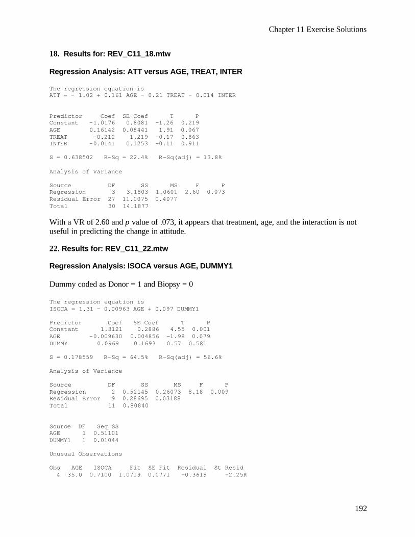
Chapter 11 Exercise Solutions
192
18. Results for: REV_C11_18.mtw Regression Analysis: ATT versus AGE, TREAT, INTER The regression equation is ATT = - 1.02 + 0.161 AGE - 0.21 TREAT - 0.014 INTER Predictor Coef SE Coef T P Constant -1.0176 0.8081 -1.26 0.219 AGE 0.16142 0.08441 1.91 0.067 TREAT -0.212 1.219 -0.17 0.863 INTER -0.0141 0.1253 -0.11 0.911 S = 0.638502 R-Sq = 22.4% R-Sq(adj) = 13.8% Analysis of Variance Source DF SS MS F P Regression 3 3.1803 1.0601 2.60 0.073 Residual Error 27 11.0075 0.4077 Total 30 14.1877 With a VR of 2.60 and p value of .073, it appears that treatment, age, and the interaction is not useful in predicting the change in attitude. 22. Results for: REV_C11_22.mtw Regression Analysis: ISOCA versus AGE, DUMMY1 Dummy coded as Donor = 1 and Biopsy = 0 The regression equation is ISOCA = 1.31 - 0.00963 AGE + 0.097 DUMMY1 Predictor Coef SE Coef T P Constant 1.3121 0.2886 4.55 0.001 AGE -0.009630 0.004856 -1.98 0.079 DUMMY 0.0969 0.1693 0.57 0.581 S = 0.178559 R-Sq = 64.5% R-Sq(adj) = 56.6% Analysis of Variance Source DF SS MS F P Regression 2 0.52145 0.26073 8.18 0.009 Residual Error 9 0.28695 0.03188 Total 11 0.80840 Source DF Seq SS AGE 1 0.51101 DUMMY1 1 0.01044 Unusual Observations Obs AGE ISOCA Fit SE Fit Residual St Resid 4 35.0 0.7100 1.0719 0.0771 -0.3619 -2.25R
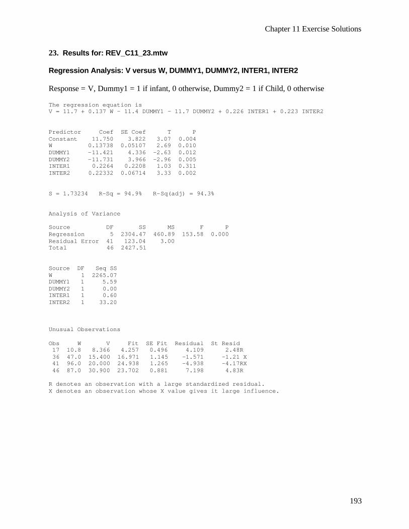
Chapter 11 Exercise Solutions
193
23. Results for: REV_C11_23.mtw Regression Analysis: V versus W, DUMMY1, DUMMY2, INTER1, INTER2 Response = V, Dummy1 = 1 if infant, 0 otherwise, Dummy2 = 1 if Child, 0 otherwise The regression equation is V = 11.7 + 0.137 W - 11.4 DUMMY1 - 11.7 DUMMY2 + 0.226 INTER1 + 0.223 INTER2 Predictor Coef SE Coef T P Constant 11.750 3.822 3.07 0.004 W 0.13738 0.05107 2.69 0.010 DUMMY1 -11.421 4.336 -2.63 0.012 DUMMY2 -11.731 3.966 -2.96 0.005 INTER1 0.2264 0.2208 1.03 0.311 INTER2 0.22332 0.06714 3.33 0.002 S = 1.73234 R-Sq = 94.9% R-Sq(adj) = 94.3% Analysis of Variance Source DF SS MS F P Regression 5 2304.47 460.89 153.58 0.000 Residual Error 41 123.04 3.00 Total 46 2427.51 Source DF Seq SS W 1 2265.07 DUMMY1 1 5.59 DUMMY2 1 0.00 INTER1 1 0.60 INTER2 1 33.20 Unusual Observations Obs W V Fit SE Fit Residual St Resid 17 10.8 8.366 4.257 0.496 4.109 2.48R 36 47.0 15.400 16.971 1.145 -1.571 -1.21 X 41 96.0 20.000 24.938 1.265 -4.938 -4.17RX 46 87.0 30.900 23.702 0.881 7.198 4.83R R denotes an observation with a large standardized residual. X denotes an observation whose X value gives it large influence.
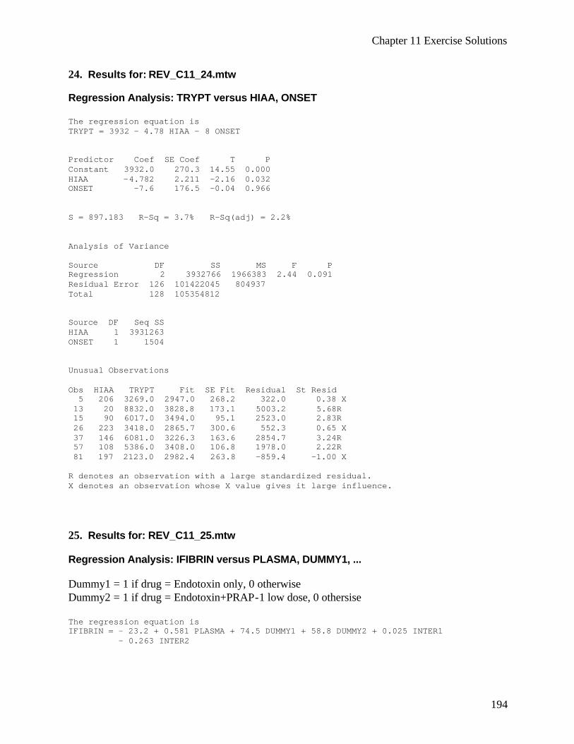
Chapter 11 Exercise Solutions
194
24. Results for: REV_C11_24.mtw Regression Analysis: TRYPT versus HIAA, ONSET The regression equation is TRYPT = 3932 - 4.78 HIAA - 8 ONSET Predictor Coef SE Coef T P Constant 3932.0 270.3 14.55 0.000 HIAA -4.782 2.211 -2.16 0.032 ONSET -7.6 176.5 -0.04 0.966 S = 897.183 R-Sq = 3.7% R-Sq(adj) = 2.2% Analysis of Variance Source DF SS MS F P Regression 2 3932766 1966383 2.44 0.091 Residual Error 126 101422045 804937 Total 128 105354812 Source DF Seq SS HIAA 1 3931263 ONSET 1 1504 Unusual Observations Obs HIAA TRYPT Fit SE Fit Residual St Resid 5 206 3269.0 2947.0 268.2 322.0 0.38 X 13 20 8832.0 3828.8 173.1 5003.2 5.68R 15 90 6017.0 3494.0 95.1 2523.0 2.83R 26 223 3418.0 2865.7 300.6 552.3 0.65 X 37 146 6081.0 3226.3 163.6 2854.7 3.24R 57 108 5386.0 3408.0 106.8 1978.0 2.22R 81 197 2123.0 2982.4 263.8 -859.4 -1.00 X R denotes an observation with a large standardized residual. X denotes an observation whose X value gives it large influence. 25. Results for: REV_C11_25.mtw Regression Analysis: IFIBRIN versus PLASMA, DUMMY1, ... Dummy1 = 1 if drug = Endotoxin only, 0 otherwise Dummy2 = 1 if drug = Endotoxin+PRAP-1 low dose, 0 othersise The regression equation is IFIBRIN = - 23.2 + 0.581 PLASMA + 74.5 DUMMY1 + 58.8 DUMMY2 + 0.025 INTER1 - 0.263 INTER2

Chapter 11 Exercise Solutions
195
Predictor Coef SE Coef T P Constant -23.22 47.32 -0.49 0.628 PLASMA 0.5808 0.3058 1.90 0.070 DUMMY1 74.46 60.53 1.23 0.231 DUMMY2 58.78 66.52 0.88 0.386 INTER1 0.0247 0.3479 0.07 0.944 INTER2 -0.2627 0.3906 -0.67 0.508 S = 41.1074 R-Sq = 72.2% R-Sq(adj) = 66.4% Analysis of Variance Source DF SS MS F P Regression 5 105331 21066 12.47 0.000 Residual Error 24 40556 1690 Total 29 145887 Source DF Seq SS PLASMA 1 68519 DUMMY1 1 34427 DUMMY2 1 707 INTER1 1 914 INTER2 1 764 Unusual Observations Obs PLASMA IFIBRIN Fit SE Fit Residual St Resid 9 414 272.00 301.89 35.73 -29.89 -1.47 X 13 248 187.00 114.43 20.14 72.57 2.03R 18 276 17.00 123.33 25.72 -106.33 -3.32R R denotes an observation with a large standardized residual. X denotes an observation whose X value gives it large influence.
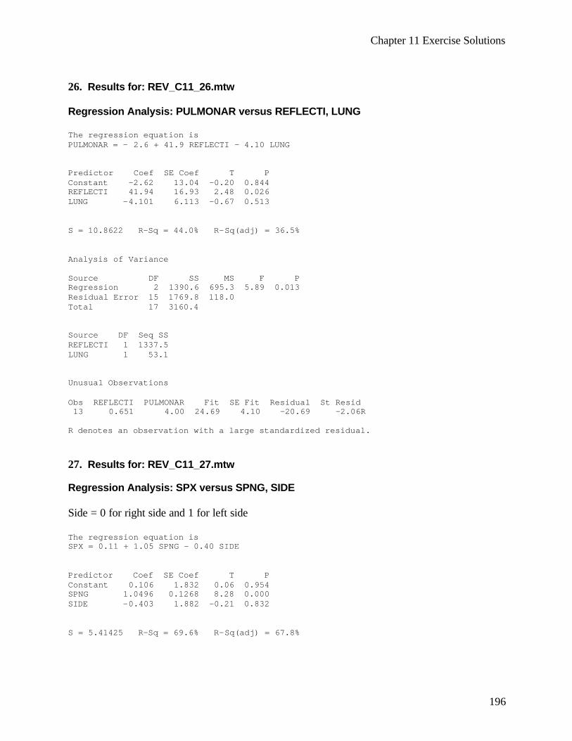
Chapter 11 Exercise Solutions
196
26. Results for: REV_C11_26.mtw Regression Analysis: PULMONAR versus REFLECTI, LUNG The regression equation is PULMONAR = - 2.6 + 41.9 REFLECTI - 4.10 LUNG Predictor Coef SE Coef T P Constant -2.62 13.04 -0.20 0.844 REFLECTI 41.94 16.93 2.48 0.026 LUNG -4.101 6.113 -0.67 0.513 S = 10.8622 R-Sq = 44.0% R-Sq(adj) = 36.5% Analysis of Variance Source DF SS MS F P Regression 2 1390.6 695.3 5.89 0.013 Residual Error 15 1769.8 118.0 Total 17 3160.4 Source DF Seq SS REFLECTI 1 1337.5 LUNG 1 53.1 Unusual Observations Obs REFLECTI PULMONAR Fit SE Fit Residual St Resid 13 0.651 4.00 24.69 4.10 -20.69 -2.06R R denotes an observation with a large standardized residual. 27. Results for: REV_C11_27.mtw Regression Analysis: SPX versus SPNG, SIDE Side = 0 for right side and 1 for left side The regression equation is SPX = 0.11 + 1.05 SPNG - 0.40 SIDE Predictor Coef SE Coef T P Constant 0.106 1.832 0.06 0.954 SPNG 1.0496 0.1268 8.28 0.000 SIDE -0.403 1.882 -0.21 0.832 S = 5.41425 R-Sq = 69.6% R-Sq(adj) = 67.8%
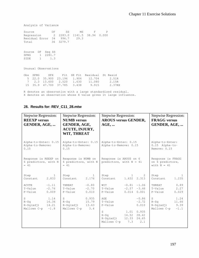
Chapter 11 Exercise Solutions
197
Analysis of Variance Source DF SS MS F P Regression 2 2283.0 1141.5 38.94 0.000 Residual Error 34 996.7 29.3 Total 36 3279.7 Source DF Seq SS SPNG 1 2281.7 SIDE 1 1.3 Unusual Observations Obs SPNG SPX Fit SE Fit Residual St Resid 5 22.0 35.900 23.196 1.904 12.704 2.51R 7 2.3 13.600 2.520 1.630 11.080 2.15R 15 35.9 47.700 37.785 3.438 9.915 2.37RX R denotes an observation with a large standardized residual. X denotes an observation whose X value gives it large influence. 28. Results for: REV_C11_28.mtw Stepwise Regression: REEXP versus GENDER, AGE, ... Alpha-to-Enter: 0.15 Alpha-to-Remove: 0.15 Response is REEXP on 6 predictors, with N = 41 Step 1 Constant 2.833 ACUTE -1.11 T-Value -2.76 P-Value 0.009 S 1.14 R-Sq 16.36 R-Sq(adj) 14.21 Mallows C-p -1.8
Stepwise Regression: NUMB versus GENDER, AGE, ACUTE, INJURY, WIT, THREAT Alpha-to-Enter: 0.15 Alpha-to-Remove: 0.15 Response is NUMB on 6 predictors, with N = 41 Step 1 Constant 2.176 THREAT -0.80 T-Value -2.70 P-Value 0.010 S 0.935 R-Sq 15.79 R-Sq(adj) 13.63 Mallows C-p 3.4
Stepwise Regression: AROUS versus GENDER, AGE, ... Alpha-to-Enter: 0.15 Alpha-to-Remove: 0.15 Response is AROUS on 6 predictors, with N = 41 Step 1 2 Constant 1.632 2.313 WIT -0.81 -1.06 T-Value -2.57 -3.46 P-Value 0.014 0.001 AGE -0.86 T-Value -2.72 P-Value 0.010 S 1.01 0.935 R-Sq 14.52 28.42 R-Sq(adj) 12.33 24.65 Mallows C-p 7.3 2.1
Stepwise Regression: FRAGG versus GENDER, AGE, ... Alpha-to-Enter: 0.15 Alpha-to-Remove: 0.15 Response is FRAGG on 6 predictors, with N = 41 Step 1 Constant 1.235 THREAT 0.89 T-Value 2.27 P-Value 0.029 S 1.24 R-Sq 11.66 R-Sq(adj) 9.39 Mallows C-p -1.1
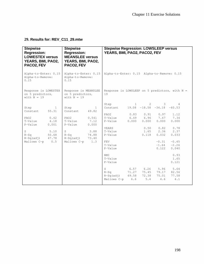
Chapter 11 Exercise Solutions
198
29. Results for: REV_C11_29.mtw Stepwise Regression: LOWESTEX versus YEARS, BMI, PAO2, PACO2, FEV Alpha-to-Enter: 0.15 Alpha-to-Remove: 0.15 Response is LOWESTEX on 5 predictors, with N = 19 Step 1 Constant 55.31 PAO2 0.42 T-Value 4.18 P-Value 0.001 S 5.10 R-Sq 50.68 R-Sq(adj) 47.78 Mallows C-p 0.5
Stepwise Regression: MEANSLEE versus YEARS, BMI, PAO2, PACO2, FEV Alpha-to-Enter: 0.15 Alpha-to-Remove: 0.15 Response is MEANSLEE on 5 predictors, with N = 19 Step 1 Constant 49.82 PAO2 0.541 T-Value 7.12 P-Value 0.000 S 3.88 R-Sq 74.88 R-Sq(adj) 73.40 Mallows C-p 1.3
Stepwise Regression: LOWSLEEP versus YEARS, BMI, PAO2, PACO2, FEV Alpha-to-Enter: 0.15 Alpha-to-Remove: 0.15 Response is LOWSLEEP on 5 predictors, with N = 19 Step 1 2 3 4 Constant 19.08 -18.58 -34.18 -60.53 PAO2 0.83 0.91 0.97 1.12 T-Value 6.49 6.96 7.47 7.34 P-Value 0.000 0.000 0.000 0.000 YEARS 0.50 0.82 0.78 T-Value 1.65 2.36 2.37 P-Value 0.118 0.032 0.033 FEV -0.31 -0.45 T-Value -1.64 -2.26 P-Value 0.122 0.040 BMI 0.93 T-Value 1.65 P-Value 0.121 S 6.57 6.26 5.96 5.64 R-Sq 71.27 75.45 79.17 82.56 R-Sq(adj) 69.58 72.38 75.01 77.58 Mallows C-p 6.6 5.4 4.6 4.1
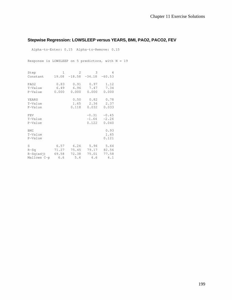
Chapter 11 Exercise Solutions
199
Stepwise Regression: LOWSLEEP versus YEARS, BMI, PAO2, PACO2, FEV Alpha-to-Enter: 0.15 Alpha-to-Remove: 0.15 Response is LOWSLEEP on 5 predictors, with N = 19 Step 1 2 3 4 Constant 19.08 -18.58 -34.18 -60.53 PAO2 0.83 0.91 0.97 1.12 T-Value 6.49 6.96 7.47 7.34 P-Value 0.000 0.000 0.000 0.000 YEARS 0.50 0.82 0.78 T-Value 1.65 2.36 2.37 P-Value 0.118 0.032 0.033 FEV -0.31 -0.45 T-Value -1.64 -2.26 P-Value 0.122 0.040 BMI 0.93 T-Value 1.65 P-Value 0.121 S 6.57 6.26 5.96 5.64 R-Sq 71.27 75.45 79.17 82.56 R-Sq(adj) 69.58 72.38 75.01 77.58 Mallows C-p 6.6 5.4 4.6 4.1
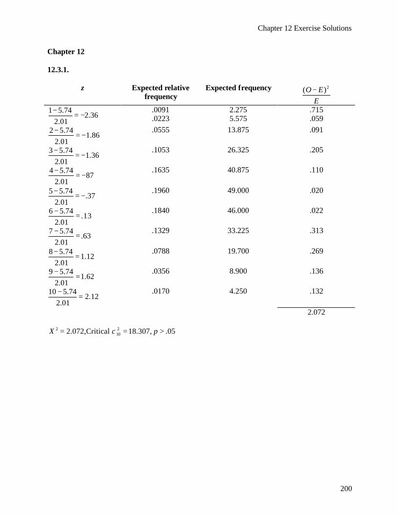
Chapter 12 Exercise Solutions
200
Chapter 12 12.3.1.
z Expected relative frequency
Expected frequency 2( )O EE−
1 5.742.36
2.01−
= − .0091 .0223
2.275 5.575
.715
.059 2 5.74
1.862.01−
= − .0555 13.875 .091
3 5.741.36
2.01−
= − .1053 26.325 .205
4 5.7487
2.01−
= − .1635 40.875 .110
5 5.74.37
2.01−
= − .1960 49.000 .020
6 5.74.13
2.01−
= .1840 46.000 .022
7 5.74.63
2.01−
= .1329 33.225 .313
8 5.741.12
2.01−
= .0788 19.700 .269
9 5.741.62
2.01−
= .0356 8.900 .136
10 5.742.12
2.01−
= .0170 4.250 .132
2.072
2 2102.072,Critical 18.307, .05X pχ= = >
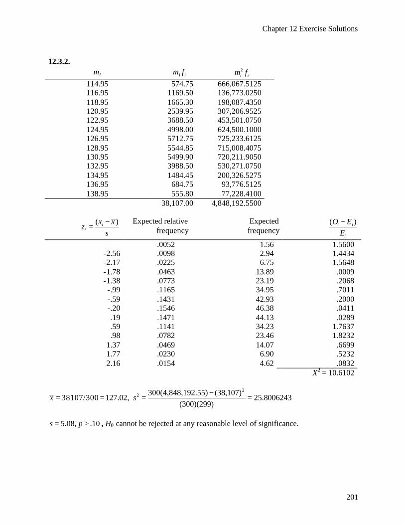
Chapter 12 Exercise Solutions
201
12.3.2.
im i im f 2i im f
114.95 574.75 666,067.5125 116.95 1169.50 136,773.0250 118.95 1665.30 198,087.4350 120.95 2539.95 307,206.9525 122.95 3688.50 453,501.0750 124.95 4998.00 624,500.1000 126.95 5712.75 725,233.6125 128.95 5544.85 715,008.4075 130.95 5499.90 720,211.9050 132.95 3988.50 530,271.0750 134.95 1484.45 200,326.5275 136.95 684.75 93,776.5125 138.95 555.80 77,228.4100
38,107.00 4,848,192.5500
( )ii
x xz
s−
= Expected relative
frequency Expected frequency
( )i i
i
O EE−
.0052 1.56 1.5600 -2.56 .0098 2.94 1.4434 -2.17 .0225 6.75 1.5648 -1.78 .0463 13.89 .0009 -1.38 .0773 23.19 .2068 -.99 .1165 34.95 .7011 -.59 .1431 42.93 .2000 -.20 .1546 46.38 .0411 .19 .1471 44.13 .0289 .59 .1141 34.23 1.7637 .98 .0782 23.46 1.8232
1.37 .0469 14.07 .6699 1.77 .0230 6.90 .5232 2.16 .0154 4.62 .0832
X2 = 10.6102
22 300(4,848,192.55) (38,107)
38107/300 127.02, 25.8006243(300)(299)
x s−
= = = =
5.08, .10s p= > , H0 cannot be rejected at any reasonable level of significance.
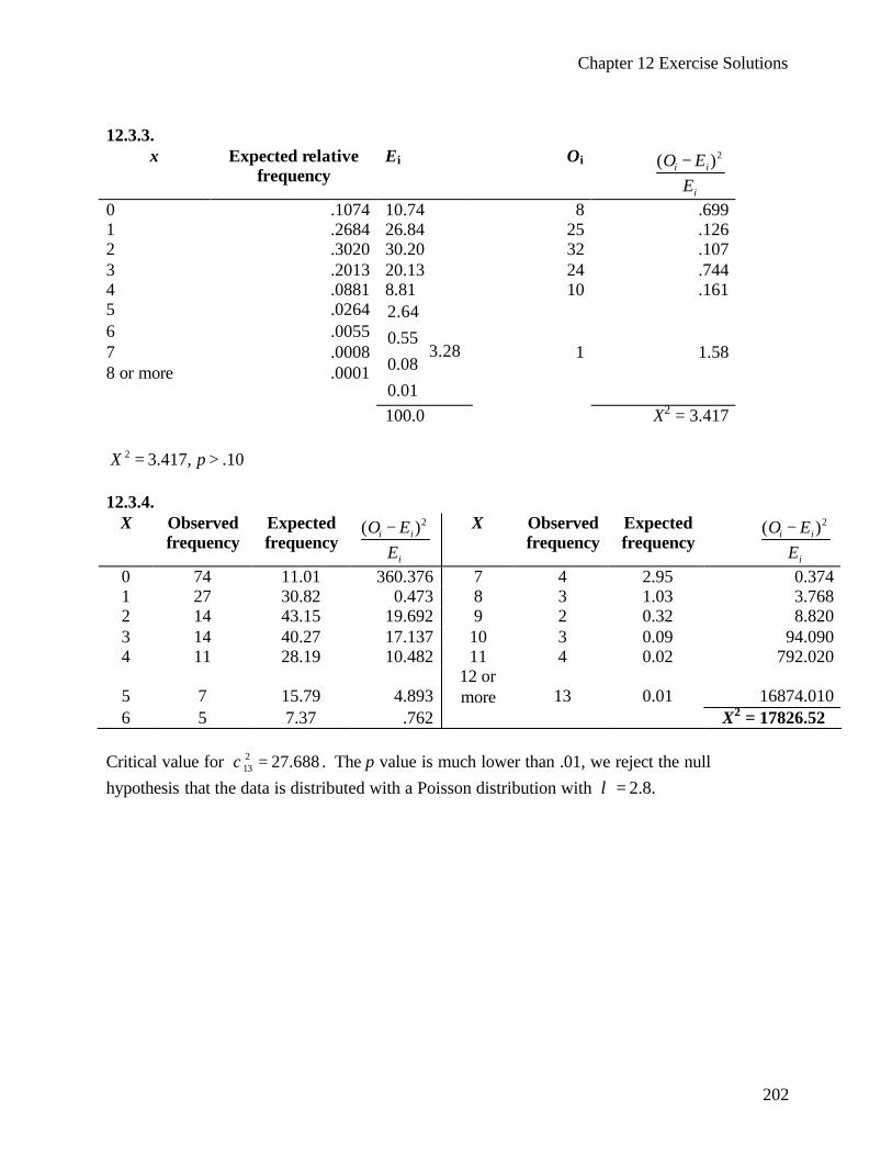
Chapter 12 Exercise Solutions
202
12.3.3.
x Expected relative frequency
Ei Oi 2( )i i
i
O EE−
0 .1074 10.74 8 .699 1 .2684 26.84 25 .126 2 .3020 30.20 32 .107 3 .2013 20.13 24 .744 4 .0881 8.81 10 .161 5 .0264 6 .0055 7 .0008 1 1.58 8 or more .0001
2.640.55
3.280.080.01
100.0 X2 = 3.417
2 3.417, .10X p= > 12.3.4.
X Observed frequency
Expected frequency
2( )i i
i
O EE−
X Observed
frequency Expected frequency
2( )i i
i
O EE−
0 74 11.01 360.376 7 4 2.95 0.374 1 27 30.82 0.473 8 3 1.03 3.768 2 14 43.15 19.692 9 2 0.32 8.820 3 14 40.27 17.137 10 3 0.09 94.090 4 11 28.19 10.482 11 4 0.02 792.020
5 7 15.79 4.893 12 or more 13 0.01 16874.010
6 5 7.37 .762 X2 = 17826.52 Critical value for 2
13 27.688χ = . The p value is much lower than .01, we reject the null hypothesis that the data is distributed with a Poisson distribution with 2.8.λ =
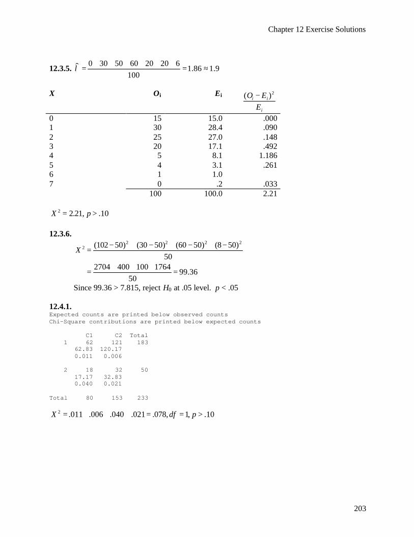
Chapter 12 Exercise Solutions
203
12.3.5. $ 0 30 50 60 20 20 61.86 1.9
100λ
+ + + + + += = ≈
X Oi Ei 2( )i i
i
O EE−
0 15 15.0 .000 1 30 28.4 .090 2 25 27.0 .148 3 20 17.1 .492 4 5 8.1 1.186 5 4 3.1 .261 6 1 1.0 7 0 .2 .033 100 100.0 2.21
2 2.21, .10X p= > 12.3.6.
2 2 2 22 (102 50) (30 50) (60 50) (8 50)
502704 400 100 1764
99.3650
X− + − + − + −
=
+ + += =
Since 99.36 > 7.815, reject H0 at .05 level. p < .05
12.4.1. Expected counts are printed below observed counts Chi-Square contributions are printed below expected counts C1 C2 Total 1 62 121 183 62.83 120.17 0.011 0.006 2 18 32 50 17.17 32.83 0.040 0.021 Total 80 153 233
2 .011 .006 .040 .021 .078, 1, .10X df p= + + + = = >

Chapter 12 Exercise Solutions
204
12.4.2. Expected counts are printed below observed counts Chi-Square contributions are printed below expected counts C1 C2 Total 1 14 94 108 9.30 98.70 2.373 0.224 2 4 97 101 8.70 92.30 2.538 0.239 Total 18 191 209 Chi-Sq = 5.374, DF = 1, P-Value = 0.020 There is sufficient evidence to reject the null hypothesis. 12.4.3. Expected counts are printed below observed counts Chi-Square contributions are printed below expected counts C1 C2 Total 1 294 921 1215 77.26 1137.74 608.095 41.291 2 98 2862 2960 188.21 2771.79 43.238 2.936 3 50 3064 3114 198.00 2916.00 110.628 7.512 4 203 2652 2855 181.53 2673.47 2.538 0.172 Total 645 9499 10144 Chi-Sq = 816.410, DF = 3, P-Value = 0.000 There is sufficient evidence to reject the null hypothesis.
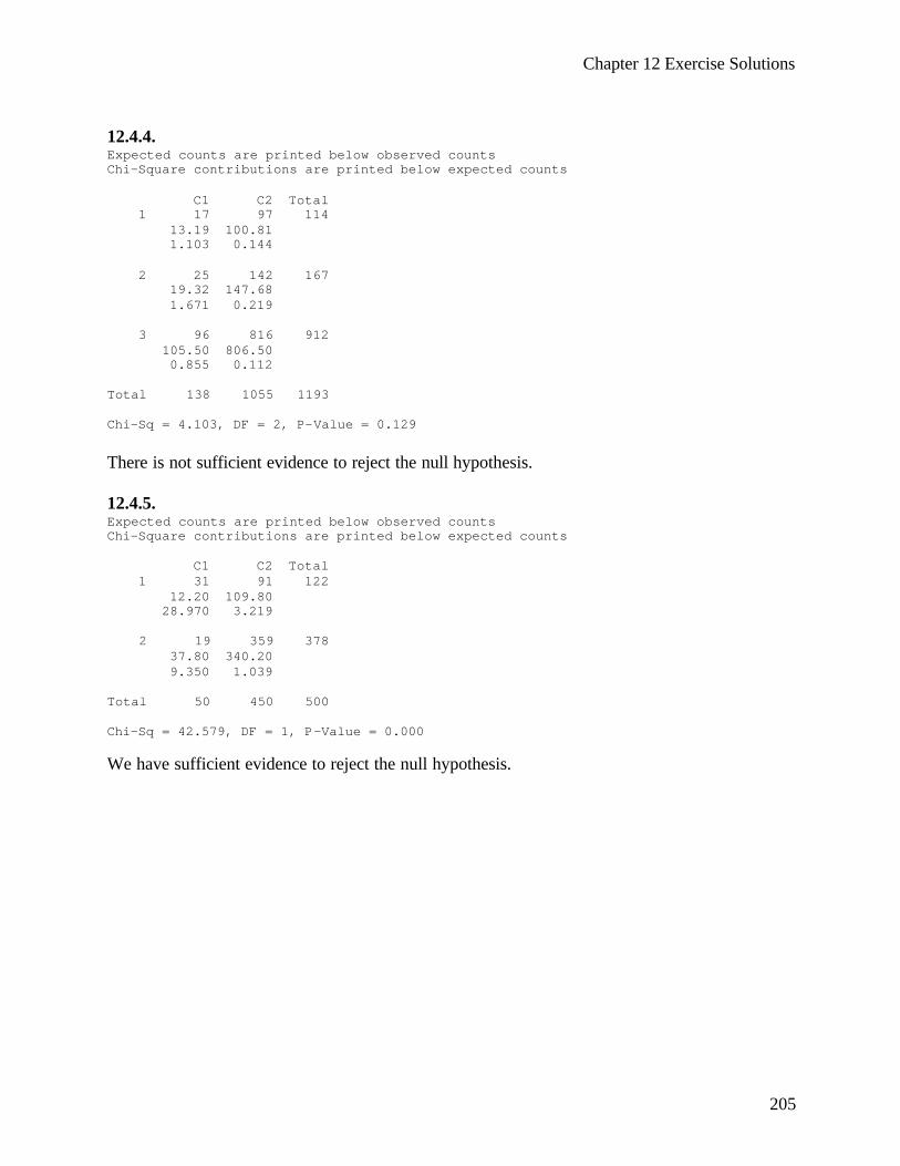
Chapter 12 Exercise Solutions
205
12.4.4. Expected counts are printed below observed counts Chi-Square contributions are printed below expected counts C1 C2 Total 1 17 97 114 13.19 100.81 1.103 0.144 2 25 142 167 19.32 147.68 1.671 0.219 3 96 816 912 105.50 806.50 0.855 0.112 Total 138 1055 1193 Chi-Sq = 4.103, DF = 2, P-Value = 0.129 There is not sufficient evidence to reject the null hypothesis. 12.4.5. Expected counts are printed below observed counts Chi-Square contributions are printed below expected counts C1 C2 Total 1 31 91 122 12.20 109.80 28.970 3.219 2 19 359 378 37.80 340.20 9.350 1.039 Total 50 450 500 Chi-Sq = 42.579, DF = 1, P-Value = 0.000 We have sufficient evidence to reject the null hypothesis.
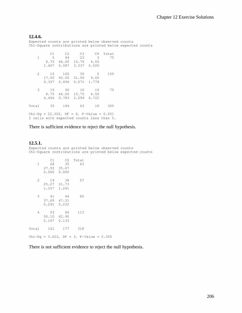
Chapter 12 Exercise Solutions
206
12.4.6. Expected counts are printed below observed counts Chi-Square contributions are printed below expected counts C1 C2 C3 C4 Total 1 5 44 23 3 75 8.75 46.00 15.75 4.50 1.607 0.087 3.337 0.500 2 15 100 30 5 150 17.50 92.00 31.50 9.00 0.357 0.696 0.071 1.778 3 15 40 10 10 75 8.75 46.00 15.75 4.50 4.464 0.783 2.099 6.722 Total 35 184 63 18 300 Chi-Sq = 22.502, DF = 6, P-Value = 0.001 2 cells with expected counts less than 5. There is sufficient evidence to reject the null hypothesis. 12.5.1. Expected counts are printed below observed counts Chi-Square contributions are printed below expected counts C1 C2 Total 1 28 35 63 27.93 35.07 0.000 0.000 2 19 38 57 25.27 31.73 1.557 1.241 3 41 44 85 37.69 47.31 0.291 0.232 4 53 60 113 50.10 62.90 0.167 0.133 Total 141 177 318 Chi-Sq = 3.622, DF = 3, P-Value = 0.305 There is not sufficient evidence to reject the null hypothesis.
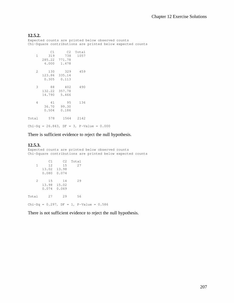
Chapter 12 Exercise Solutions
207
12.5.2. Expected counts are printed below observed counts Chi-Square contributions are printed below expected counts C1 C2 Total 1 319 738 1057 285.22 771.78 4.000 1.478 2 130 329 459 123.86 335.14 0.305 0.113 3 88 402 490 132.22 357.78 14.790 5.466 4 41 95 136 36.70 99.30 0.504 0.186 Total 578 1564 2142 Chi-Sq = 26.843, DF = 3, P-Value = 0.000 There is sufficient evidence to reject the null hypothesis. 12.5.3. Expected counts are printed below observed counts Chi-Square contributions are printed below expected counts C1 C2 Total 1 12 15 27 13.02 13.98 0.080 0.074 2 15 14 29 13.98 15.02 0.074 0.069 Total 27 29 56 Chi-Sq = 0.297, DF = 1, P-Value = 0.586 There is not sufficient evidence to reject the null hypothesis.
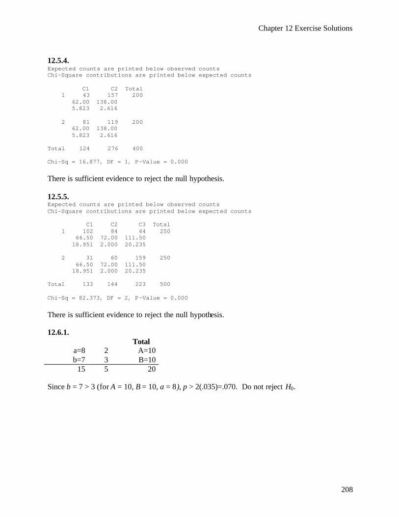
Chapter 12 Exercise Solutions
208
12.5.4. Expected counts are printed below observed counts Chi-Square contributions are printed below expected counts C1 C2 Total 1 43 157 200 62.00 138.00 5.823 2.616 2 81 119 200 62.00 138.00 5.823 2.616 Total 124 276 400 Chi-Sq = 16.877, DF = 1, P-Value = 0.000 There is sufficient evidence to reject the null hypothesis. 12.5.5. Expected counts are printed below observed counts Chi-Square contributions are printed below expected counts C1 C2 C3 Total 1 102 84 64 250 66.50 72.00 111.50 18.951 2.000 20.235 2 31 60 159 250 66.50 72.00 111.50 18.951 2.000 20.235 Total 133 144 223 500 Chi-Sq = 82.373, DF = 2, P-Value = 0.000 There is sufficient evidence to reject the null hypothesis. 12.6.1. Total
a=8 2 A=10 b=7 3 B=10
15 5 20 Since b = 7 > 3 (for A = 10, B = 10, a = 8), p > 2(.035)=.070. Do not reject H0.

Chapter 12 Exercise Solutions
209
12.6.2. Total
a=8 2 A=10 b=2 8 B=10
10 10 20 Since b = 2 (for A = 10, B = 10, a = 8), p = 2(.012) = .024. Reject H0. 12.6.3. Total
a=16 3 A=19 b=1 6 B=7
17 9 26 Since b = 1 (for A = 19, B = 7, a = 16), p = 2(.002) = .004. Reject H0. 12.7.1. Survival No Yes Total
Age 50 or older 219 157 376 Younger than 50 16 355 371
Total 235 512 747
¶ 219/37613.51
16/371RR = = ,
22 747(219*355 157*16)
241.3048(235)(512)(376)(371)
X−
= =
95% CI: 1 1.96/ 241.3048 11.96/ 241.304813.51 9.7,13.51 18.76− += = There is statistically significant evidence that older subjects do not survive at a higher rate than younger subjects. The 95% CI generated by SAS® is 8.30, 21.98
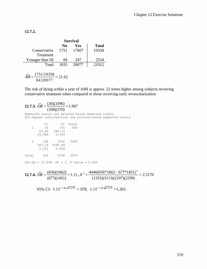
Chapter 12 Exercise Solutions
210
12.7.2. Survival No Yes Total
Conservative Treatment
1751 17607 19358
Younger than 50 84 247 2554 Total 1835 20077 21912
¶ 1751/1935821.62
84/20077RR = =
The risk of dying within a year of AMI is approx. 22 times higher among subjects receiving conservative treatment when compared to those receiving early revascularization.
12.7.3. ¶ (36)(3396)1.967
(168)(370)OR = =
Expected counts are printed below observed counts Chi-Square contributions are printed below expected counts C1 C2 Total 1 36 370 406 20.86 385.14 10.984 0.595 2 168 3396 3564 183.14 3380.86 1.251 0.068 Total 204 3766 3970 Chi-Sq = 12.898, DF = 1, P-Value = 0.000
12.7.4. ¶ (656)(1662)1.11
(677)(1451)OR = = ,
22 4446(656*1662 677*1451)
2.5170(1333)(3113)(2107)(2339)
X−
= =
95% CI: 1 1.96/ 2.5170 1 1.96/ 2.51701.11 .978, 1.11 1.263− += =

Chapter 12 Exercise Solutions
211
12.7.5.
¶(40)(38) (75)(33)
11.875 15.373128 161 3.733(13)(37) (15)(38) 3.758 3.540
128 161
MHOR+ +
= = =++
1 2 1 22 2
(77)(53) (113)(90) (77)(51)(53)(75) (113)(48)(90)(71)31.883, 63.168, 7.502, 8.357
128 161 128127 161160e e v v= = = = = = = =
2
2 [(40 75) (31.883 63.168)]25.094
7.502 8.357MHχ+ − +
= =+
Reject the null hypothesis, we conclude there is a relationship between garden ownership and food insecurity among employed and non-employed families.
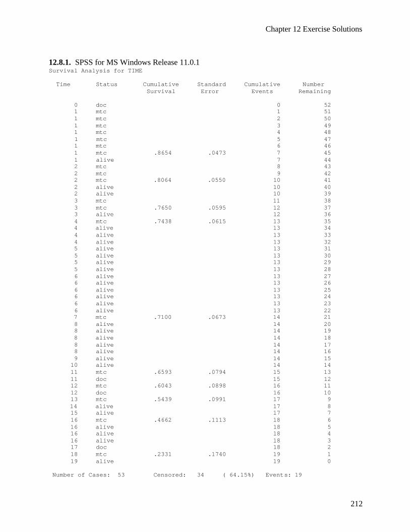
Chapter 12 Exercise Solutions
212
12.8.1. SPSS for MS Windows Release 11.0.1 Survival Analysis for TIME Time Status Cumulative Standard Cumulative Number Survival Error Events Remaining 0 doc 0 52 1 mtc 1 51 1 mtc 2 50 1 mtc 3 49 1 mtc 4 48 1 mtc 5 47 1 mtc 6 46 1 mtc .8654 .0473 7 45 1 alive 7 44 2 mtc 8 43 2 mtc 9 42 2 mtc .8064 .0550 10 41 2 alive 10 40 2 alive 10 39 3 mtc 11 38 3 mtc .7650 .0595 12 37 3 alive 12 36 4 mtc .7438 .0615 13 35 4 alive 13 34 4 alive 13 33 4 alive 13 32 5 alive 13 31 5 alive 13 30 5 alive 13 29 5 alive 13 28 6 alive 13 27 6 alive 13 26 6 alive 13 25 6 alive 13 24 6 alive 13 23 6 alive 13 22 7 mtc .7100 .0673 14 21 8 alive 14 20 8 alive 14 19 8 alive 14 18 8 alive 14 17 8 alive 14 16 9 alive 14 15 10 alive 14 14 11 mtc .6593 .0794 15 13 11 doc 15 12 12 mtc .6043 .0898 16 11 12 doc 16 10 13 mtc .5439 .0991 17 9 14 alive 17 8 15 alive 17 7 16 mtc .4662 .1113 18 6 16 alive 18 5 16 alive 18 4 16 alive 18 3 17 doc 18 2 18 mtc .2331 .1740 19 1 19 alive 19 0 Number of Cases: 53 Censored: 34 ( 64.15%) Events: 19
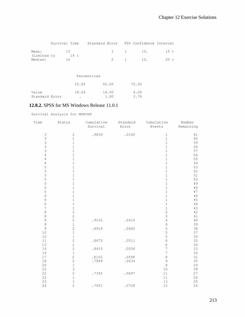
Chapter 12 Exercise Solutions
213
Survival Time Standard Error 95% Confidence Interval Mean: 13 1 ( 10, 15 ) (Limited to 19 ) Median: 16 2 ( 12, 20 ) Percentiles 25.00 50.00 75.00 Value 18.00 16.00 4.00 Standard Error . 1.80 3.76 12.8.2. SPSS for MS Windows Release 11.0.1 Survival Analysis for MONTHS Time Status Cumulative Standard Cumulative Number Survival Error Events Remaining 3 2 .9839 .0160 1 61 3 1 1 60 3 1 1 59 3 1 1 58 3 1 1 57 4 1 1 56 4 1 1 55 4 1 1 54 5 1 1 53 5 1 1 52 5 1 1 51 5 1 1 50 5 1 1 49 5 1 1 48 5 1 1 47 6 1 1 46 6 1 1 45 6 1 1 44 7 1 1 43 8 2 2 42 8 2 3 41 8 2 .9152 .0410 4 40 8 1 4 39 9 2 .8918 .0462 5 38 10 1 5 37 10 1 5 36 11 2 .8670 .0511 6 35 13 1 6 34 16 2 .8415 .0556 7 33 16 1 7 32 17 2 .8152 .0598 8 31 18 2 .7889 .0634 9 30 20 1 9 29 22 2 10 28 22 2 .7345 .0697 11 27 22 1 11 26 23 1 11 25 24 2 .7051 .0728 12 24
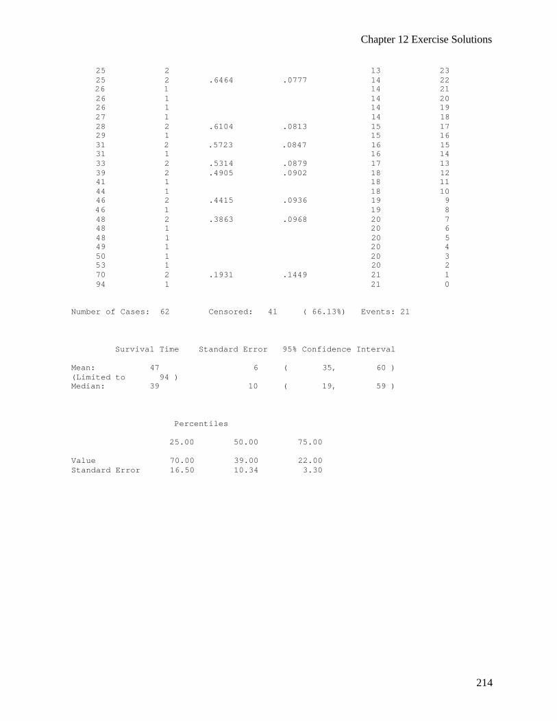
Chapter 12 Exercise Solutions
214
25 2 13 23 25 2 .6464 .0777 14 22 26 1 14 21 26 1 14 20 26 1 14 19 27 1 14 18 28 2 .6104 .0813 15 17 29 1 15 16 31 2 .5723 .0847 16 15 31 1 16 14 33 2 .5314 .0879 17 13 39 2 .4905 .0902 18 12 41 1 18 11 44 1 18 10 46 2 .4415 .0936 19 9 46 1 19 8 48 2 .3863 .0968 20 7 48 1 20 6 48 1 20 5 49 1 20 4 50 1 20 3 53 1 20 2 70 2 .1931 .1449 21 1 94 1 21 0 Number of Cases: 62 Censored: 41 ( 66.13%) Events: 21 Survival Time Standard Error 95% Confidence Interval Mean: 47 6 ( 35, 60 ) (Limited to 94 ) Median: 39 10 ( 19, 59 ) Percentiles 25.00 50.00 75.00 Value 70.00 39.00 22.00 Standard Error 16.50 10.34 3.30
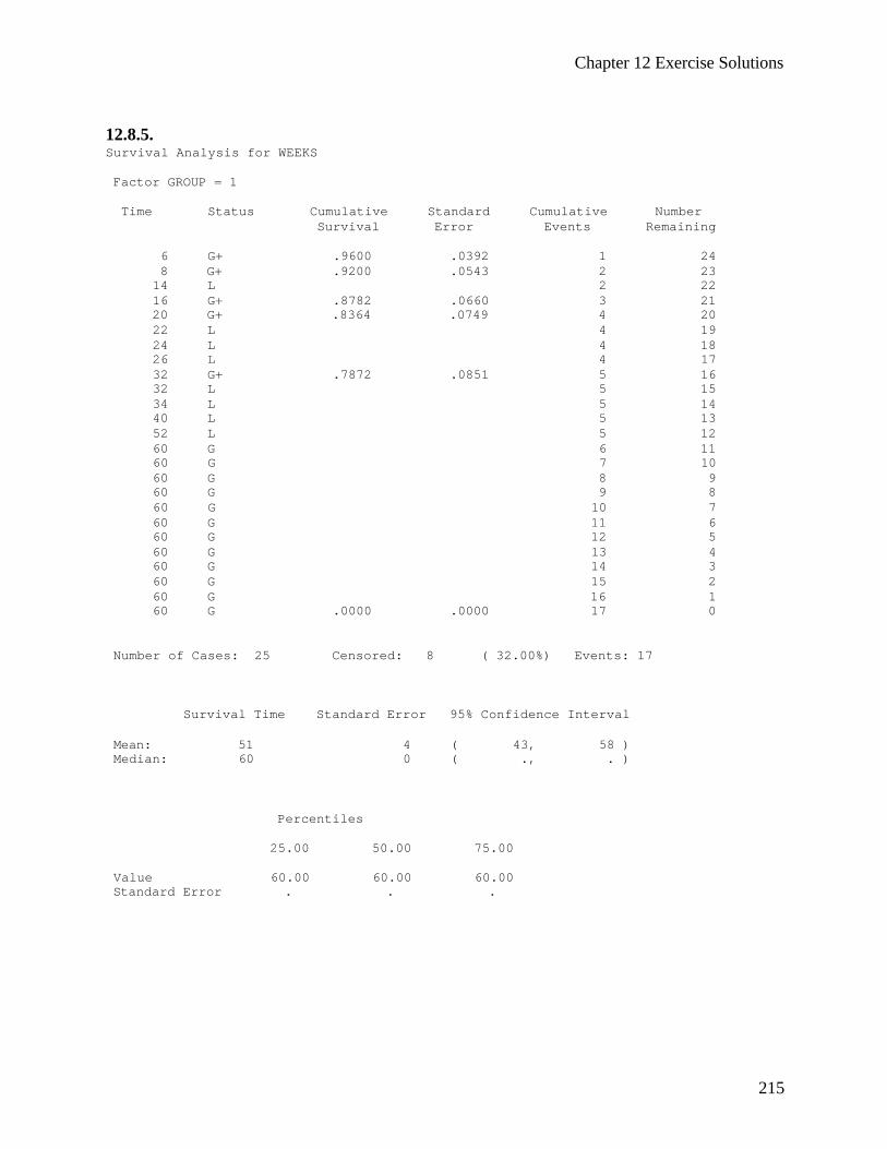
Chapter 12 Exercise Solutions
215
12.8.5. Survival Analysis for WEEKS Factor GROUP = 1 Time Status Cumulative Standard Cumulative Number Survival Error Events Remaining 6 G+ .9600 .0392 1 24 8 G+ .9200 .0543 2 23 14 L 2 22 16 G+ .8782 .0660 3 21 20 G+ .8364 .0749 4 20 22 L 4 19 24 L 4 18 26 L 4 17 32 G+ .7872 .0851 5 16 32 L 5 15 34 L 5 14 40 L 5 13 52 L 5 12 60 G 6 11 60 G 7 10 60 G 8 9 60 G 9 8 60 G 10 7 60 G 11 6 60 G 12 5 60 G 13 4 60 G 14 3 60 G 15 2 60 G 16 1 60 G .0000 .0000 17 0 Number of Cases: 25 Censored: 8 ( 32.00%) Events: 17 Survival Time Standard Error 95% Confidence Interval Mean: 51 4 ( 43, 58 ) Median: 60 0 ( ., . ) Percentiles 25.00 50.00 75.00 Value 60.00 60.00 60.00 Standard Error . . .

Chapter 12 Exercise Solutions
216
Survival Analysis for WEEKS Factor GROUP = 2 Time Status Cumulative Standard Cumulative Number Survival Error Events Remaining 2 G+ .9600 .0392 1 24 3 G+ .9200 .0543 2 23 4 G+ .8800 .0650 3 22 6 G+ .8400 .0733 4 21 7 G+ 5 20 7 G+ .7600 .0854 6 19 8 G+ 7 18 8 G+ .6800 .0933 8 17 10 G+ 9 16 10 G+ .6000 .0980 10 15 10 L 10 14 12 G+ .5571 .0999 11 13 15 G+ .5143 .1010 12 12 18 G+ .4714 .1013 13 11 18 L 13 10 20 G+ 14 9 20 G+ .3771 .1006 15 8 22 G+ 16 7 22 G+ .2829 .0950 17 6 24 G+ .2357 .0901 18 5 26 G+ .1886 .0835 19 4 27 G+ .1414 .0748 20 3 28 G+ .0943 .0630 21 2 32 G+ .0471 .0459 22 1 36 G+ .0000 .0000 23 0 Number of Cases: 25 Censored: 2 ( 8.00%) Events: 23 Survival Time Standard Error 95% Confidence Interval Mean: 17 2 ( 13, 21 ) Median: 18 5 ( 9, 27 ) Percentiles 25.00 50.00 75.00 Value 24.00 18.00 8.00 Standard Error 2.87 4.50 1.17 _ Survival Analysis for WEEKS Total Number Number Percent Events Censored Censored GROUP 1 25 17 8 32.00 GROUP 2 25 23 2 8.00 Overall 50 40 10 20.00
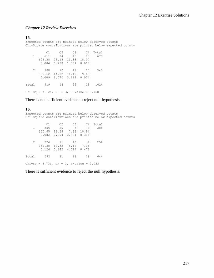
Chapter 12 Exercise Solutions
217
Chapter 12 Review Exercises 15. Expected counts are printed below observed counts Chi-Square contributions are printed below expected counts C1 C2 C3 C4 Total 1 611 34 16 18 679 609.38 29.18 21.88 18.57 0.004 0.798 1.581 0.017 2 308 10 17 10 345 309.62 14.82 11.12 9.43 0.009 1.570 3.112 0.034 Total 919 44 33 28 1024 Chi-Sq = 7.124, DF = 3, P-Value = 0.068 There is not sufficient evidence to reject null hypothesis. 16. Expected counts are printed below observed counts Chi-Square contributions are printed below expected counts C1 C2 C3 C4 Total 1 356 20 3 9 388 350.65 18.68 7.83 10.84 0.082 0.094 2.981 0.314 2 226 11 10 9 256 231.35 12.32 5.17 7.16 0.124 0.142 4.519 0.476 Total 582 31 13 18 644 Chi-Sq = 8.731, DF = 3, P-Value = 0.033 There is sufficient evidence to reject the null hypothesis.

Chapter 12 Exercise Solutions
218
17. Expected counts are printed below observed counts Chi-Square contributions are printed below expected counts C1 C2 Total 1 72 230 302 69.69 232.31 0.076 0.023 2 54 192 246 56.77 189.23 0.135 0.041 3 16 63 79 18.23 60.77 0.273 0.082 4 8 15 23 5.31 17.69 1.366 0.410 Total 150 500 650 Chi-Sq = 2.405, DF = 3, P-Value = 0.493 There is not sufficient evidence to reject the null hypothesis. 18. Expected counts are printed below observed counts Chi-Square contributions are printed below expected counts C1 C2 C3 Total 1 6 30 22 58 7.54 31.61 18.85 0.315 0.082 0.526 2 11 35 17 63 8.19 34.34 20.48 0.964 0.013 0.590 3 4 19 14 37 4.81 20.17 12.03 0.136 0.067 0.324 4 5 25 12 42 5.46 22.89 13.65 0.039 0.194 0.199 Total 26 109 65 200 Chi-Sq = 3.450, DF = 6, P-Value = 0.751 1 cells with expected counts less than 5.
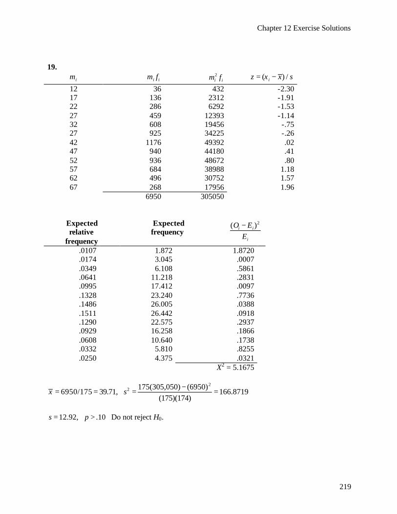
Chapter 12 Exercise Solutions
219
19.
im i im f 2i im f ( ) /iz x x s= −
12 36 432 -2.30 17 136 2312 -1.91 22 286 6292 -1.53 27 459 12393 -1.14 32 608 19456 -.75 27 925 34225 -.26 42 1176 49392 .02 47 940 44180 .41 52 936 48672 .80 57 684 38988 1.18 62 496 30752 1.57 67 268 17956 1.96
6950 305050
Expected relative
frequency
Expected frequency
2( )i i
i
O EE−
.0107 1.872 1.8720
.0174 3.045 .0007
.0349 6.108 .5861
.0641 11.218 .2831
.0995 17.412 .0097
.1328 23.240 .7736
.1486 26.005 .0388
.1511 26.442 .0918
.1290 22.575 .2937
.0929 16.258 .1866
.0608 10.640 .1738
.0332 5.810 .8255
.0250 4.375 .0321 X2 = 5.1675
2
2 175(305,050) (6950)6950/175 39.71, 166.8719
(175)(174)x s
−= = = =
12.92, .10s p= > Do not reject H0.
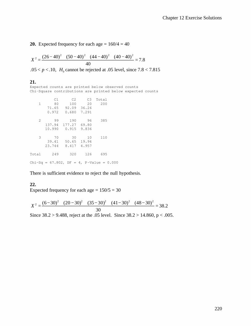
Chapter 12 Exercise Solutions
220
20. Expected frequency for each age = 160/4 = 40
2 2 2 22 (26 40) (50 40) (44 40) (40 40)
7.840
X− + − + − + −
= =
0.05 .10,p H< < cannot be rejected at .05 level, since 7.8 < 7.815 21. Expected counts are printed below observed counts Chi-Square contributions are printed below expected counts C1 C2 C3 Total 1 80 100 20 200 71.65 92.09 36.26 0.972 0.680 7.291 2 99 190 96 385 137.94 177.27 69.80 10.990 0.915 9.836 3 70 30 10 110 39.41 50.65 19.94 23.744 8.417 4.957 Total 249 320 126 695 Chi-Sq = 67.802, DF = 4, P-Value = 0.000 There is sufficient evidence to reject the null hypothesis. 22. Expected frequency for each age = 150/5 = 30
2 2 2 2 22 (6 30) (20 30) (35 30) (41 30) (48 30)
38.230
X− + − + − + − + −
= =
Since 38.2 > 9.488, reject at the .05 level. Since 38.2 > 14.860, p < .005.
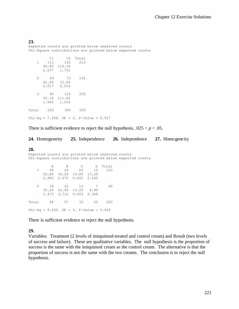
Chapter 12 Exercise Solutions
221
23. Expected counts are printed below observed counts Chi-Square contributions are printed below expected counts C1 C2 Total 1 111 102 213 96.82 116.18 2.077 1.731 2 59 73 132 60.00 72.00 0.017 0.014 3 80 125 205 93.18 111.82 1.865 1.554 Total 250 300 550 Chi-Sq = 7.258, DF = 2, P-Value = 0.027 There is sufficient evidence to reject the null hypothesis, .025 < p < .05. 24. Homogeneity 25. Independence 26. Independence 27. Homogeneity 28. Expected counts are printed below observed counts Chi-Square contributions are printed below expected counts A B C D Total 1 60 25 20 15 120 52.80 34.20 19.80 13.20 0.982 2.475 0.002 0.245 2 28 32 13 7 80 35.20 22.80 13.20 8.80 1.473 3.712 0.003 0.368 Total 88 57 33 22 200 Chi-Sq = 9.260, DF = 3, P-Value = 0.026 There is sufficient evidence to reject the null hypothesis. 29. Variables: Treatment (2 levels of imiquimod-treated and control cream) and Result (two levels of success and failure). These are qualitative variables. The null hypothesis is the proportion of success is the same with the imiquimod cream as the control cream. The alternative is that the proportion of success is not the same with the two creams. The conclusion is to reject the null hypothesis.

Chapter 12 Exercise Solutions
222
30. Variables: aneurysm size was made a qualitative variable of less than 13mm versus 13mm or greater. The outcome variable of experiencing transient/persistent neurological deficits is also qualitative. Conclusion: since the 95% confidence interval does not contain 1.0, the results are significant. One can conclude that subjects with smaller tumor sizes have significantly lower odds of having transient/persistent neurological deficits after surgery. 31. The variables are qualitative. The null hypothesis is that age and treatment choice are independent. The alternative is that they are not independent. Expected counts are printed below observed counts Chi-Square contributions are printed below expected counts NTP B NTP+B Total 1 15 26 16 57 8.14 30.46 18.40 5.774 0.653 0.312 2 6 54 40 100 14.29 53.44 32.28 4.806 0.006 1.849 3 6 21 5 32 4.57 17.10 10.33 0.446 0.889 2.749 Total 27 101 61 189 Chi-Sq = 17.485, DF = 4, P-Value = 0.002 1 cells with expected counts less than 5. There is sufficient evidence to reject the null hypothesis. 32. The results of OR = .07 indicates younger teenagers seeking abortion are significantly less likely to know about emergency contraception than older women also seeking abortion. The OR = .10 indicated the same group of younger teenagers seeking abortion is less likely to know about emergency contraception than the teenagers of similar age in the control group. The Mantel-Haenszel p value indicates a significant result stating that there is a relationship between age of subjects and whether they have knowledge of emergency contraception among both abortion seekers and the control group. 33. This is a retrospective study. The variables are qualitative with the risk factor of living in area of high road traffic exhaust and a response variable as childhood leukemia. The children living in the high exhaust areas had odds almost 4 times higher for contracting childhood leukemia than comparable children in non-traffic exhaust areas. 34. This was an observational prospective study. The variables are qualitative with the exception of age; participation is the outcome variable. Age, employment, diagnosis, stress were statistically significant.
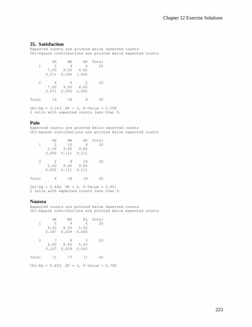
Chapter 12 Exercise Solutions
223
35. Satisfaction Expected counts are printed below observed counts Chi-Square contributions are printed below expected counts UH MH HD Total 1 5 9 6 20 7.00 9.00 4.00 0.571 0.000 1.000 2 9 9 2 20 7.00 9.00 4.00 0.571 0.000 1.000 Total 14 18 8 40 Chi-Sq = 3.143, DF = 2, P-Value = 0.208 2 cells with expected counts less than 5. Pain Expected counts are printed below observed counts Chi-Square contributions are printed below expected counts UH MH HD Total 1 2 10 8 20 2.00 9.00 9.00 0.000 0.111 0.111 2 2 8 10 20 2.00 9.00 9.00 0.000 0.111 0.111 Total 4 18 18 40 Chi-Sq = 0.444, DF = 2, P-Value = 0.801 2 cells with expected counts less than 5. Nausea Expected counts are printed below observed counts Chi-Square contributions are printed below expected counts UB MO SL Total 1 5 9 6 20 6.00 8.50 5.50 0.167 0.029 0.045 2 7 8 5 20 6.00 8.50 5.50 0.167 0.029 0.045 Total 12 17 11 40 Chi-Sq = 0.483, DF = 2, P-Value = 0.785
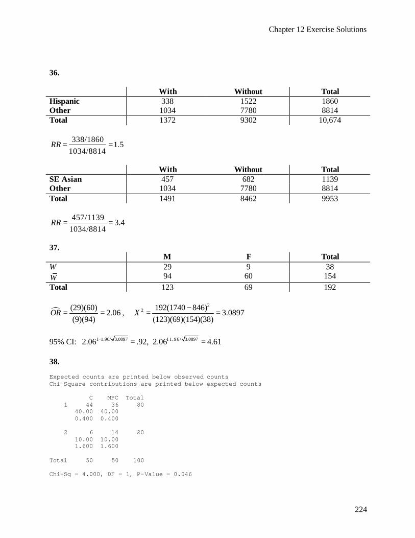
Chapter 12 Exercise Solutions
224
36. With Without Total Hispanic 338 1522 1860 Other 1034 7780 8814 Total 1372 9302 10,674
338/18601.5
1034/8814RR = =
With Without Total SE Asian 457 682 1139 Other 1034 7780 8814 Total 1491 8462 9953
457/11393.4
1034/8814RR = =
37. M F Total W 29 9 38 W 94 60 154 Total 123 69 192
¶ (29)(60)2.06
(9)(94)OR = = ,
22 192(1740 846)
3.0897(123)(69)(154)(38)
X−
= =
95% CI: 1 1.96/ 3.0897 11.96/ 3.08972.06 .92, 2.06 4.61− += = 38. Expected counts are printed below observed counts Chi-Square contributions are printed below expected counts C MPC Total 1 44 36 80 40.00 40.00 0.400 0.400 2 6 14 20 10.00 10.00 1.600 1.600 Total 50 50 100 Chi-Sq = 4.000, DF = 1, P-Value = 0.046
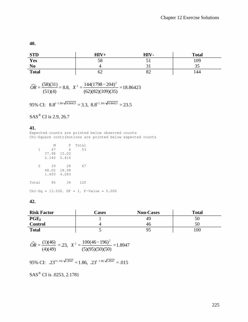
Chapter 12 Exercise Solutions
225
40. STD HIV+ HIV- Total Yes 58 51 109 No 4 31 35 Total 62 82 144
¶ 22(58)(31) 144(1798 204)
8.8, 18.86423(51)(4) (62)(82)(109)(35)
OR X−
= = = =
95% CI: 1 1.96/ 18.86423 11.96/ 18.864238.8 3.3, 8.8 23.5− += = SAS® CI is 2.9, 26.7 41. Expected counts are printed below observed counts Chi-Square contributions are printed below expected counts M F Total 1 47 6 53 37.98 15.02 2.140 5.414 2 39 28 67 48.02 18.98 1.693 4.283 Total 86 34 120 Chi-Sq = 13.530, DF = 1, P-Value = 0.000 42. Risk Factor Cases Non-Cases Total PGE2 1 49 50 Control 4 46 50 Total 5 95 100
¶ 22(1)(46) 100(46 196)
.23, 1.8947(4)(49) (5)(95)(50)(50)
OR X−
= = = =
95% CI: 1 1 . 9 6 / 1.8947 1 1.96/ 1.8947.23 1.86, .23 .015− += = SAS® CI is .0253, 2.1781

Chapter 12 Exercise Solutions
226
43. Fisher’s Exact Test Post Operative Complication
Ultrasonic Appearance of Fetal Bowel
Total
Normal Not Normal No 13 5 18 Yes 2 7 9 Total 15 12 27 Test statistic = 2, p = .019 44. Seek Shelter Total Understand No Yes No 19 10 29 Yes 46 118 164 Total 65 128 193
¶ (19)(118)4.87
(46)(10)OR = =
45. Expected counts are printed below observed counts Chi-Square contributions are printed below expected counts 40-69 >=70 Total 1 21 17 38 28.79 9.21 2.106 6.580 2 4000 1270 5270 3992.21 1277.79 0.015 0.047 Total 4021 1287 5308 Chi-Sq = 8.749, DF = 1, P-Value = 0.003
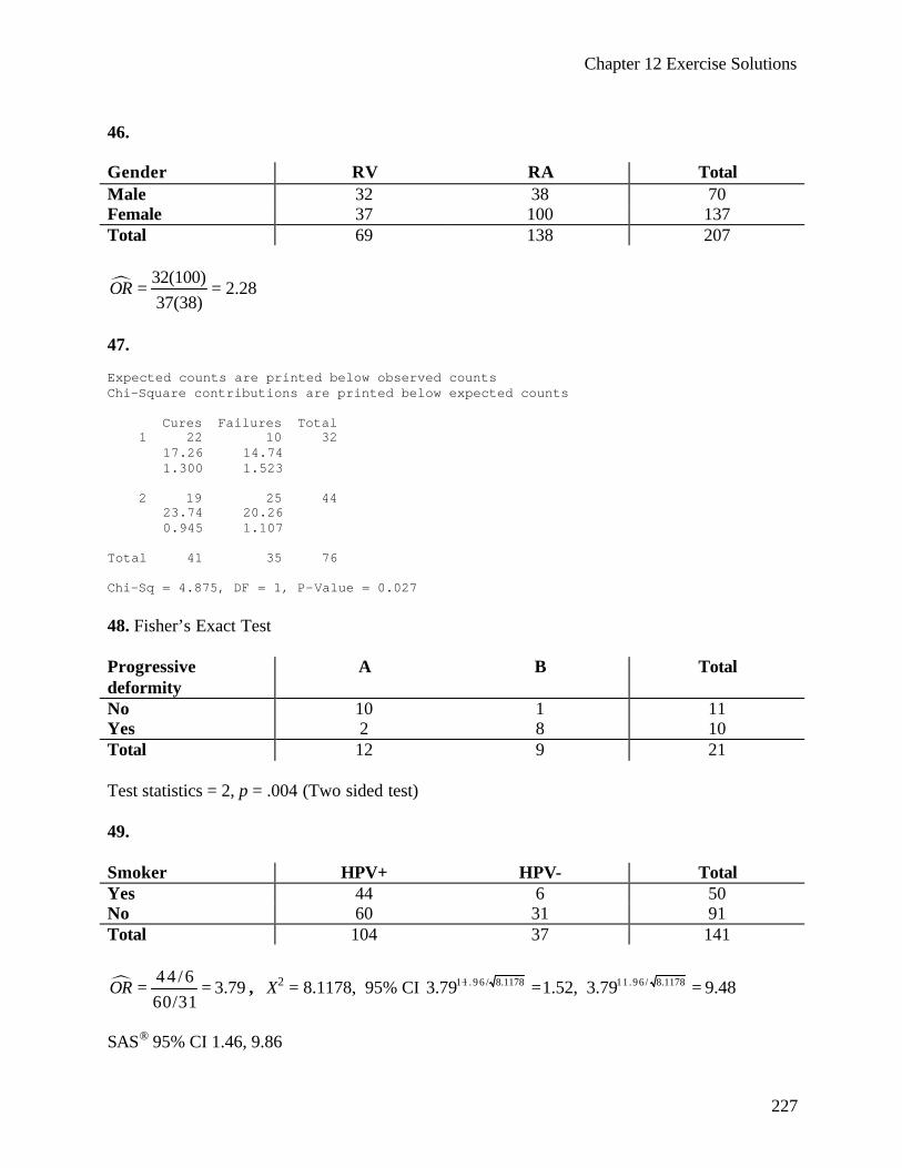
Chapter 12 Exercise Solutions
227
46. Gender RV RA Total Male 32 38 70 Female 37 100 137 Total 69 138 207
¶ 32(100)2.28
37(38)OR = =
47. Expected counts are printed below observed counts Chi-Square contributions are printed below expected counts Cures Failures Total 1 22 10 32 17.26 14.74 1.300 1.523 2 19 25 44 23.74 20.26 0.945 1.107 Total 41 35 76 Chi-Sq = 4.875, DF = 1, P-Value = 0.027 48. Fisher’s Exact Test Progressive deformity
A B Total
No 10 1 11 Yes 2 8 10 Total 12 9 21 Test statistics = 2, p = .004 (Two sided test) 49. Smoker HPV+ HPV- Total Yes 44 6 50 No 60 31 91 Total 104 37 141
¶ 44 /63.79
60/31OR = = , X2 = 8.1178, 95% CI 1 1 . 9 6 / 8.1178 11.96/ 8.11783.79 1.52, 3.79 9.48− += =
SAS® 95% CI 1.46, 9.86
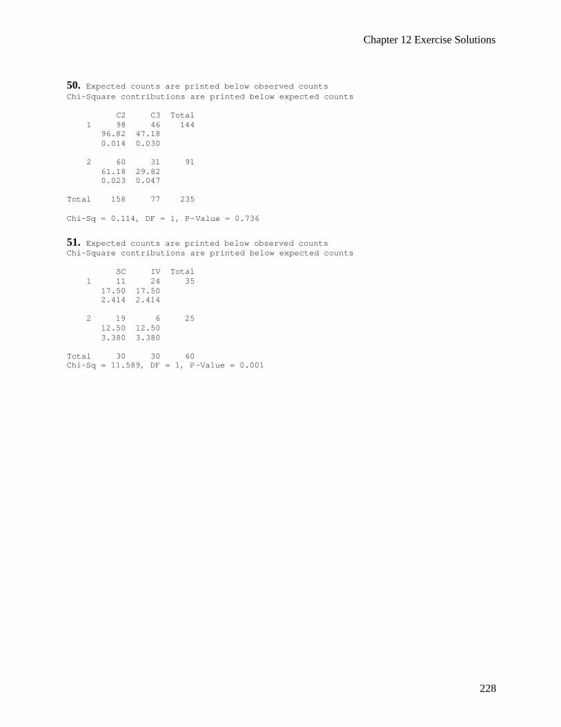
Chapter 12 Exercise Solutions
228
50. Expected counts are printed below observed counts Chi-Square contributions are printed below expected counts C2 C3 Total 1 98 46 144 96.82 47.18 0.014 0.030 2 60 31 91 61.18 29.82 0.023 0.047 Total 158 77 235 Chi-Sq = 0.114, DF = 1, P-Value = 0.736 51. Expected counts are printed below observed counts Chi-Square contributions are printed below expected counts SC IV Total 1 11 24 35 17.50 17.50 2.414 2.414 2 19 6 25 12.50 12.50 3.380 3.380 Total 30 30 60 Chi-Sq = 11.589, DF = 1, P-Value = 0.001

Chapter 12 Exercise Solutions
229
52. Survival Analysis for DAYS Factor GRADE = 0 Time Status Cumulative Standard Cumulative Number Survival Error Events Remaining 87 0 0 39 775 0 0 38 881 0 0 37 914 0 0 36 1155 0 0 35 1162 0 0 34 1271 0 0 33 1616 0 0 32 1982 0 0 31 2035 0 0 30 2191 0 0 29 2472 0 0 28 2527 0 0 27 2782 0 0 26 3108 0 0 25 3158 0 0 24 3609 0 0 23 3772 0 0 22 3799 0 0 21 3819 0 0 20 4586 0 0 19 4680 0 0 18 4989 0 0 17 5675 0 0 16 5936 0 0 15 5985 0 0 14 6175 0 0 13 6177 0 0 12 6214 0 0 11 6225 0 0 10 6449 0 0 9 6669 0 0 8 6685 0 0 7 6873 0 0 6 6951 0 0 5 7318 0 0 4 7447 0 0 3 9525 0 0 2 9938 0 0 1 10429 0 0 0 >Warning # 20077. Command name: KM >Survival estimates cannot be computed since all observations are censored.
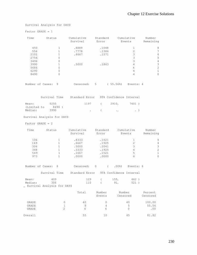
Chapter 12 Exercise Solutions
230
Survival Analysis for DAYS Factor GRADE = 1 Time Status Cumulative Standard Cumulative Number Survival Error Events Remaining 450 1 .8889 .1048 1 8 556 1 .7778 .1386 2 7 2102 1 .6667 .1571 3 6 2756 0 3 5 3496 0 3 4 3990 1 .5000 .1863 4 3 5686 0 4 2 6290 0 4 1 8490 0 4 0 Number of Cases: 9 Censored: 5 ( 55.56%) Events: 4 Survival Time Standard Error 95% Confidence Interval Mean: 5255 1197 ( 2910, 7601 ) (Limited to 8490 ) Median: 3990 . ( ., . ) Survival Analysis for DAYS Factor GRADE = 2 Time Status Cumulative Standard Cumulative Number Survival Error Events Remaining 106 1 .8333 .1521 1 5 169 1 .6667 .1925 2 4 306 1 .5000 .2041 3 3 348 1 .3333 .1925 4 2 549 1 .1667 .1521 5 1 973 1 .0000 .0000 6 0 Number of Cases: 6 Censored: 0 ( .00%) Events: 6 Survival Time Standard Error 95% Confidence Interval Mean: 409 129 ( 155, 662 ) Median: 306 110 ( 91, 521 ) _ Survival Analysis for DAYS Total Number Number Percent Events Censored Censored GRADE 0 40 0 40 100.00 GRADE 1 9 4 5 55.56 GRADE 2 6 6 0 .00 Overall 55 10 45 81.82
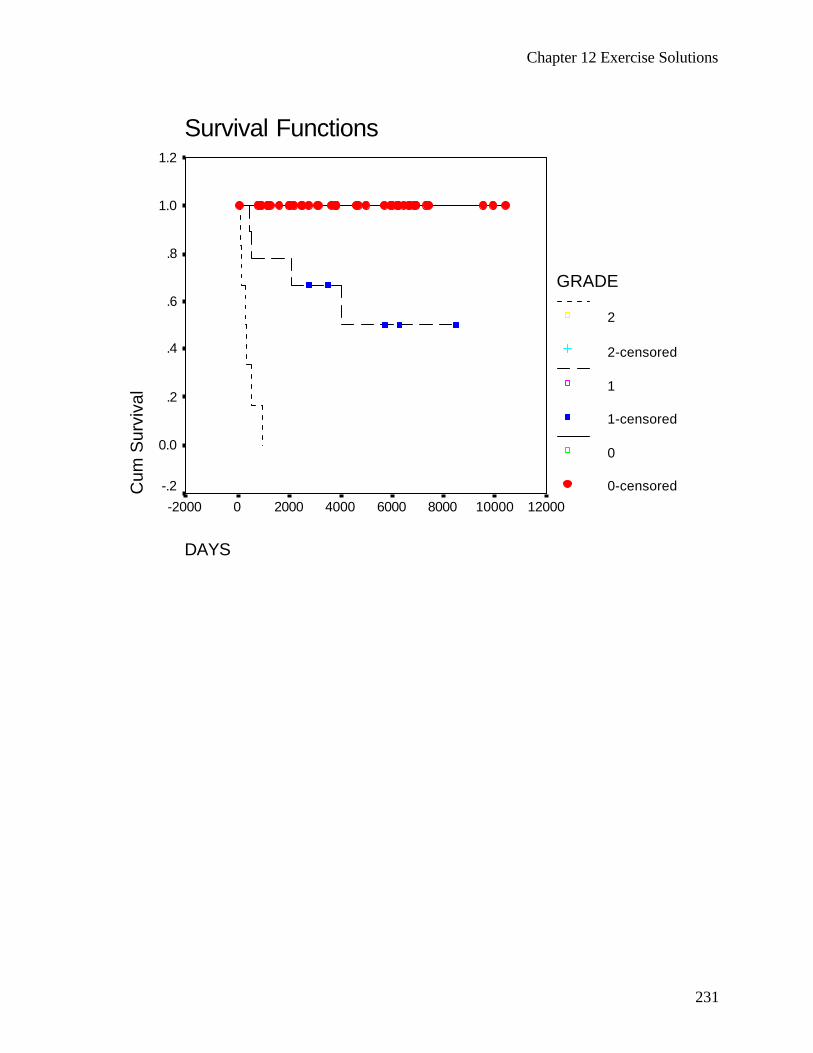
Chapter 12 Exercise Solutions
231
Survival Functions
DAYS
120001000080006000400020000-2000
Cum
Sur
viva
l1.2
1.0
.8
.6
.4
.2
0.0
-.2
GRADE
2
2-censored
1
1-censored
0
0-censored
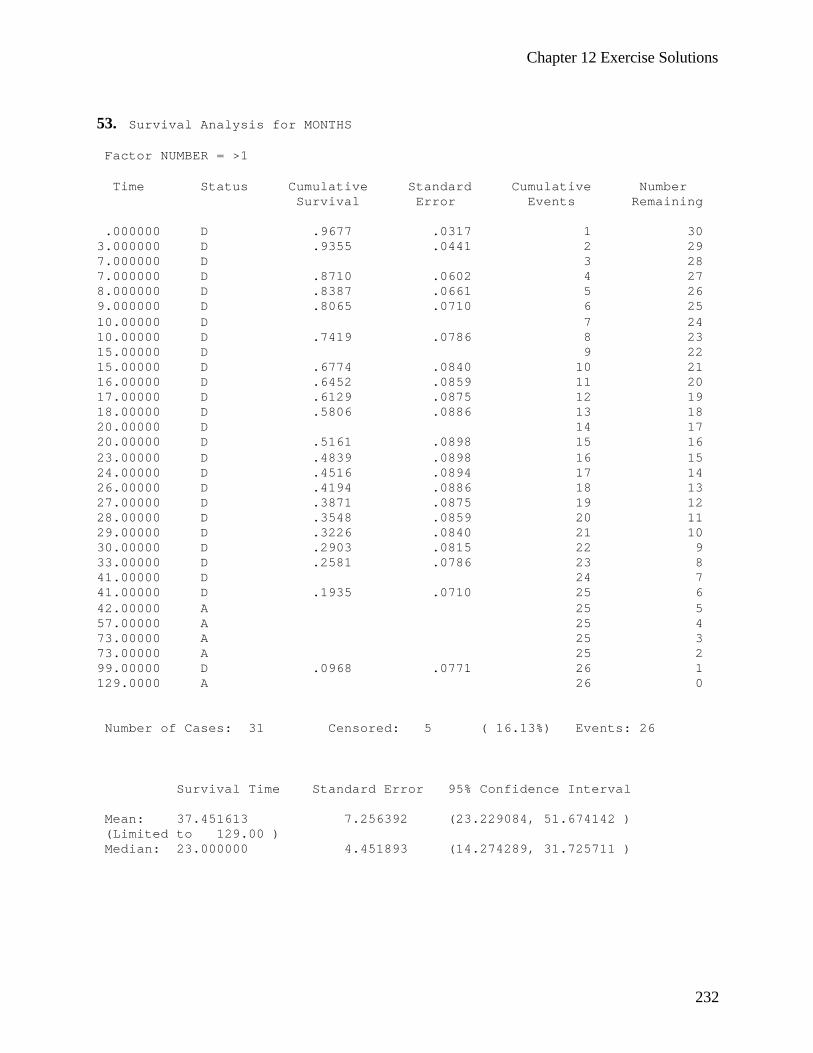
Chapter 12 Exercise Solutions
232
53. Survival Analysis for MONTHS Factor NUMBER = >1 Time Status Cumulative Standard Cumulative Number Survival Error Events Remaining .000000 D .9677 .0317 1 30 3.000000 D .9355 .0441 2 29 7.000000 D 3 28 7.000000 D .8710 .0602 4 27 8.000000 D .8387 .0661 5 26 9.000000 D .8065 .0710 6 25 10.00000 D 7 24 10.00000 D .7419 .0786 8 23 15.00000 D 9 22 15.00000 D .6774 .0840 10 21 16.00000 D .6452 .0859 11 20 17.00000 D .6129 .0875 12 19 18.00000 D .5806 .0886 13 18 20.00000 D 14 17 20.00000 D .5161 .0898 15 16 23.00000 D .4839 .0898 16 15 24.00000 D .4516 .0894 17 14 26.00000 D .4194 .0886 18 13 27.00000 D .3871 .0875 19 12 28.00000 D .3548 .0859 20 11 29.00000 D .3226 .0840 21 10 30.00000 D .2903 .0815 22 9 33.00000 D .2581 .0786 23 8 41.00000 D 24 7 41.00000 D .1935 .0710 25 6 42.00000 A 25 5 57.00000 A 25 4 73.00000 A 25 3 73.00000 A 25 2 99.00000 D .0968 .0771 26 1 129.0000 A 26 0 Number of Cases: 31 Censored: 5 ( 16.13%) Events: 26 Survival Time Standard Error 95% Confidence Interval Mean: 37.451613 7.256392 (23.229084, 51.674142 ) (Limited to 129.00 ) Median: 23.000000 4.451893 (14.274289, 31.725711 )

Chapter 12 Exercise Solutions
233
Survival Analysis for MONTHS Factor NUMBER = 1 Time Status Cumulative Standard Cumulative Number Survival Error Events Remaining 2.000000 D .9783 .0215 1 45 3.000000 A 1 44 5.000000 D .9560 .0304 2 43 10.00000 D 3 42 10.00000 D .9116 .0422 4 41 14.00000 D .8893 .0467 5 40 15.00000 D 6 39 15.00000 D .8449 .0539 7 38 16.00000 D .8226 .0569 8 37 17.00000 D 9 36 17.00000 D .7782 .0619 10 35 18.00000 D .7559 .0640 11 34 19.00000 D .7337 .0659 12 33 19.00000 A 12 32 24.00000 A 12 31 24.00000 A 12 30 26.00000 D 13 29 26.00000 D .6848 .0700 14 28 27.00000 D 15 27 27.00000 D .6359 .0730 16 26 29.00000 D .6114 .0742 17 25 29.00000 A 17 24 33.00000 D .5859 .0753 18 23 35.00000 A 18 22 37.00000 D .5593 .0765 19 21 39.00000 A 19 20 40.00000 A 19 19 41.00000 D .5299 .0779 20 18 42.00000 A 20 17 43.00000 D 21 16 43.00000 D .4675 .0803 22 15 45.00000 A 22 14 46.00000 D .4341 .0812 23 13 54.00000 D .4007 .0815 24 12 55.00000 A 24 11 60.00000 D .3643 .0818 25 10 66.00000 A 25 9 67.00000 A 25 8 74.00000 A 25 7 92.00000 A 25 6 93.00000 A 25 5 121.0000 A 25 4 127.0000 A 25 3 133.0000 A 25 2 143.0000 A 25 1 169.0000 A 25 0
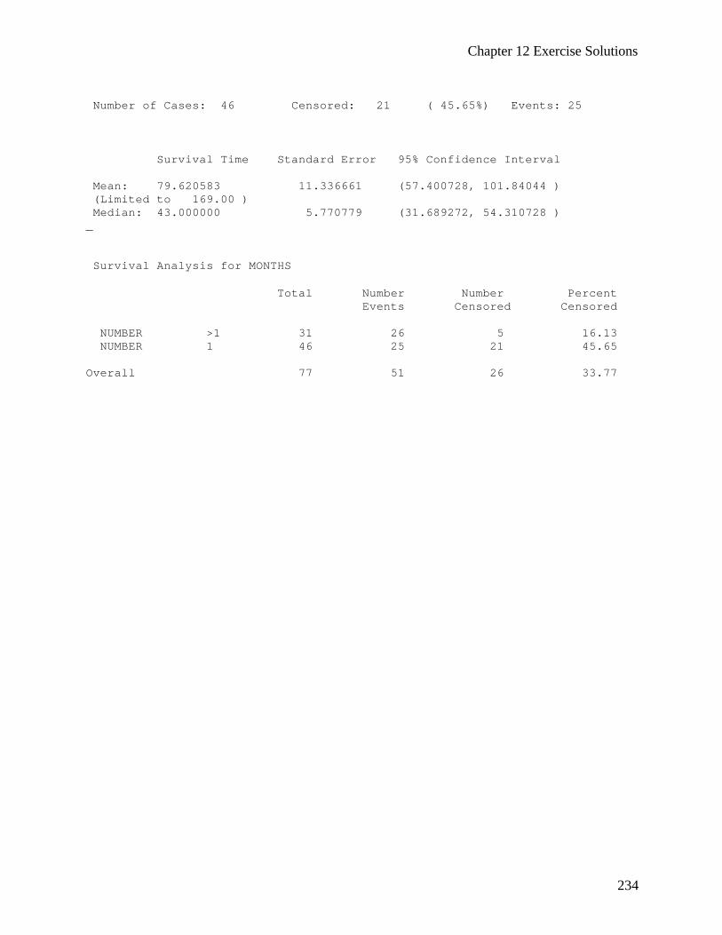
Chapter 12 Exercise Solutions
234
Number of Cases: 46 Censored: 21 ( 45.65%) Events: 25 Survival Time Standard Error 95% Confidence Interval Mean: 79.620583 11.336661 (57.400728, 101.84044 ) (Limited to 169.00 ) Median: 43.000000 5.770779 (31.689272, 54.310728 ) _ Survival Analysis for MONTHS Total Number Number Percent Events Censored Censored NUMBER >1 31 26 5 16.13 NUMBER 1 46 25 21 45.65 Overall 77 51 26 33.77

Chapter 13 Exercise Solutions
235
Chapter 13 13.3.1. H0: median = 100, HA: median ≠100
Sign of x – 100: -, -, -, +, +, -, +, -, -, +, -, +, +, -, -
( 6|15,.5) .3036, 2(.3036) .6072P k p≤ = = = , fail to reject the null hypothesis. 13.3.2. Subtract concentration with water from concentration taken with grapefruit juice.
0 : ( ) ( ), : ( ) ( )AH p p H p p+ ≤ − + > − , Number of +’s = 4.
( 4 | 7, .5) .50P x n p≥ = = = 13.3.3. Subj 1 2 3 4 5 6 7 8 9 10 11 12 13 14 15 B-A 0 + - - 0 - - - + - - - - - -
( 2|13,.5) .0112P x ≤ = , reject the null hypothesis 13.4.1.
70i id x= − Signed Rank of di
-7 -14.5 -2 -2 9 16
-5 -8.5 -6 -11.5 -7 -14.5 -5 -8.5 -6 -11.5 6 11.5 4 6
-4 -6 -4 -6 -3 -3.5 3 3.5
-1 -1 6 11.5
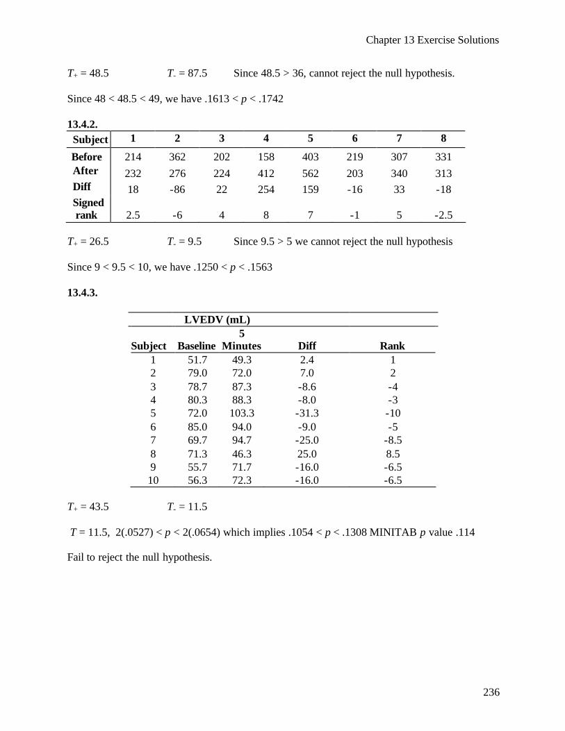
Chapter 13 Exercise Solutions
236
T+ = 48.5 T- = 87.5 Since 48.5 > 36, cannot reject the null hypothesis. Since 48 < 48.5 < 49, we have .1613 < p < .1742 13.4.2. Subject 1 2 3 4 5 6 7 8
Before 214 362 202 158 403 219 307 331 After 232 276 224 412 562 203 340 313 Diff 18 -86 22 254 159 -16 33 -18 Signed rank 2.5 -6 4 8 7 -1 5 -2.5 T+ = 26.5 T- = 9.5 Since 9.5 > 5 we cannot reject the null hypothesis Since 9 < 9.5 < 10, we have .1250 < p < .1563 13.4.3.
LVEDV (mL)
Subject Baseline 5
Minutes Diff Rank 1 51.7 49.3 2.4 1 2 79.0 72.0 7.0 2 3 78.7 87.3 -8.6 -4 4 80.3 88.3 -8.0 -3 5 72.0 103.3 -31.3 -10 6 85.0 94.0 -9.0 -5 7 69.7 94.7 -25.0 -8.5 8 71.3 46.3 25.0 8.5 9 55.7 71.7 -16.0 -6.5 10 56.3 72.3 -16.0 -6.5
T+ = 43.5 T- = 11.5 T = 11.5, 2(.0527) < p < 2(.0654) which implies .1054 < p < .1308 MINITAB p value .114 Fail to reject the null hypothesis.

Chapter 13 Exercise Solutions
237
13.5.1. Median = 79.5 Hospital A B Total Above Median 13 2 15 Below Median 2 13 15 Total 15 15 30
22 30(13*13 2*2)
16.13333(15)(15)(15)(15)
X−
= = Since 16.13333 > 3.841, reject the null hypothesis, p < .005
13.5.2. Median = 3.3 Normal Hospitalized Total Above Median 12 3 15 Below Median 5 10 15 Total 17 13 30
22 30(12*10 5*3)
6.652(17)(13)(15)(15)
X−
= = Since 6.652 > 3.841, reject the null hypothesis that the
medians are equal, .005 < p < .01 13.6.1. Sum of the ranks for group 1 is 1378.5 and for group 2 it is 1106.5. Let S = 1378.5 and
thus 34(35)
1378.5 712.52
T = − = . Since both groups have sample sizes greater than 20, we use
712.5 [(36)(34)/2]1.18
36(34)(36 34 1)/12z
−= =
+ +, which yields a two sided p value of .1190(2) = .2380. We
fail to reject H0. 13.6.2. Sum of the ranks for group 1 is 48 and for group 2 it is 105. Let S = 48 and thus
8(9)48 12
2T = − = . Using Table L we find the critical value to be 12 at α =.05, so we fail to
reject H0. The 2-sided p value is greater than .02. 13.6.3. Sum of the ranks for group 1 is 1772.50 and for group 2 it is 1713.5. Let S = 1772.50 and
thus 43(44)
1772.5 826.52
T = − = . Since both groups have sample sizes greater than 20, we use
826.5 [(43)(40)/2].31
43(40)(43 40 1)/12z
−= = −
+ +. The 2-sided p value is 2(.3783) = .7566. Fail to reject H0.

Chapter 13 Exercise Solutions
238
13.7.1.
x ( 1050)/50z x= − ( )TF x Freq 859 -3.82 0.0001 1904 -2.92 0.0018 1920 -2.60 0.0047 1962 -1.76 0.0392 1973 -1.54 0.0618 1
1001 -0.98 0.1635 11002 -0.96 0.1695 11012 -0.76 0.2236 11016 -0.68 0.2483 11039 -0.22 0.4192 11041 -0.18 0.4286 11051 0.02 0.5080 11064 0.28 0.6103 11073 0.46 0.6772 11086 0.72 0.7642 11117 1.34 0.9099 11140 1.80 0.9641 11141 1.82 0.9656 11146 1.92 0.9726 11166 2.32 0.9898 11168 2.36 0.9909 11202 3.04 0.9988 11233 3.66 ≅1.0000 11255 4.10 ≅1.0000 11348 5.96 ≅1.0000 1
25
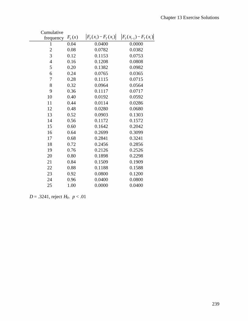
Chapter 13 Exercise Solutions
239
Cumulative frequency ( )SF x ( ) ( )S i T iF x F x− 1( ) ( )S i T iF x F x− −
1 0.04 0.0400 0.0000 2 0.08 0.0782 0.0382 3 0.12 0.1153 0.0753 4 0.16 0.1208 0.0808 5 0.20 0.1382 0.0982 6 0.24 0.0765 0.0365 7 0.28 0.1115 0.0715 8 0.32 0.0964 0.0564 9 0.36 0.1117 0.0717
10 0.40 0.0192 0.0592 11 0.44 0.0114 0.0286 12 0.48 0.0280 0.0680 13 0.52 0.0903 0.1303 14 0.56 0.1172 0.1572 15 0.60 0.1642 0.2042 16 0.64 0.2699 0.3099 17 0.68 0.2841 0.3241 18 0.72 0.2456 0.2856 19 0.76 0.2126 0.2526 20 0.80 0.1898 0.2298 21 0.84 0.1509 0.1909 22 0.88 0.1188 0.1588 23 0.92 0.0800 0.1200 24 0.96 0.0400 0.0800 25 1.00 0.0000 0.0400
D = .3241, reject H0. p < .01
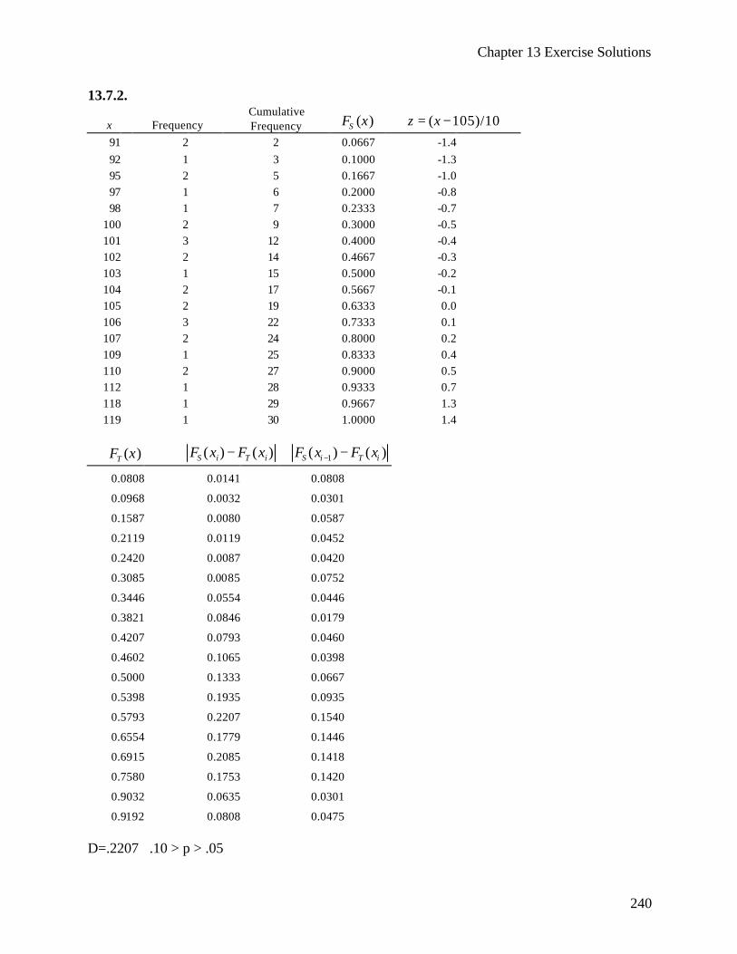
Chapter 13 Exercise Solutions
240
13.7.2.
x Frequency Cumulative Frequency ( )SF x ( 105)/10z x= −
91 2 2 0.0667 -1.4 92 1 3 0.1000 -1.3 95 2 5 0.1667 -1.0 97 1 6 0.2000 -0.8 98 1 7 0.2333 -0.7
100 2 9 0.3000 -0.5 101 3 12 0.4000 -0.4 102 2 14 0.4667 -0.3 103 1 15 0.5000 -0.2 104 2 17 0.5667 -0.1 105 2 19 0.6333 0.0 106 3 22 0.7333 0.1 107 2 24 0.8000 0.2 109 1 25 0.8333 0.4 110 2 27 0.9000 0.5 112 1 28 0.9333 0.7 118 1 29 0.9667 1.3 119 1 30 1.0000 1.4
( )TF x ( ) ( )S i T iF x F x− 1( ) ( )S i T iF x F x− −
0.0808 0.0141 0.0808
0.0968 0.0032 0.0301
0.1587 0.0080 0.0587
0.2119 0.0119 0.0452
0.2420 0.0087 0.0420
0.3085 0.0085 0.0752
0.3446 0.0554 0.0446
0.3821 0.0846 0.0179
0.4207 0.0793 0.0460
0.4602 0.1065 0.0398
0.5000 0.1333 0.0667
0.5398 0.1935 0.0935
0.5793 0.2207 0.1540
0.6554 0.1779 0.1446
0.6915 0.2085 0.1418
0.7580 0.1753 0.1420
0.9032 0.0635 0.0301
0.9192 0.0808 0.0475 D=.2207 .10 > p > .05
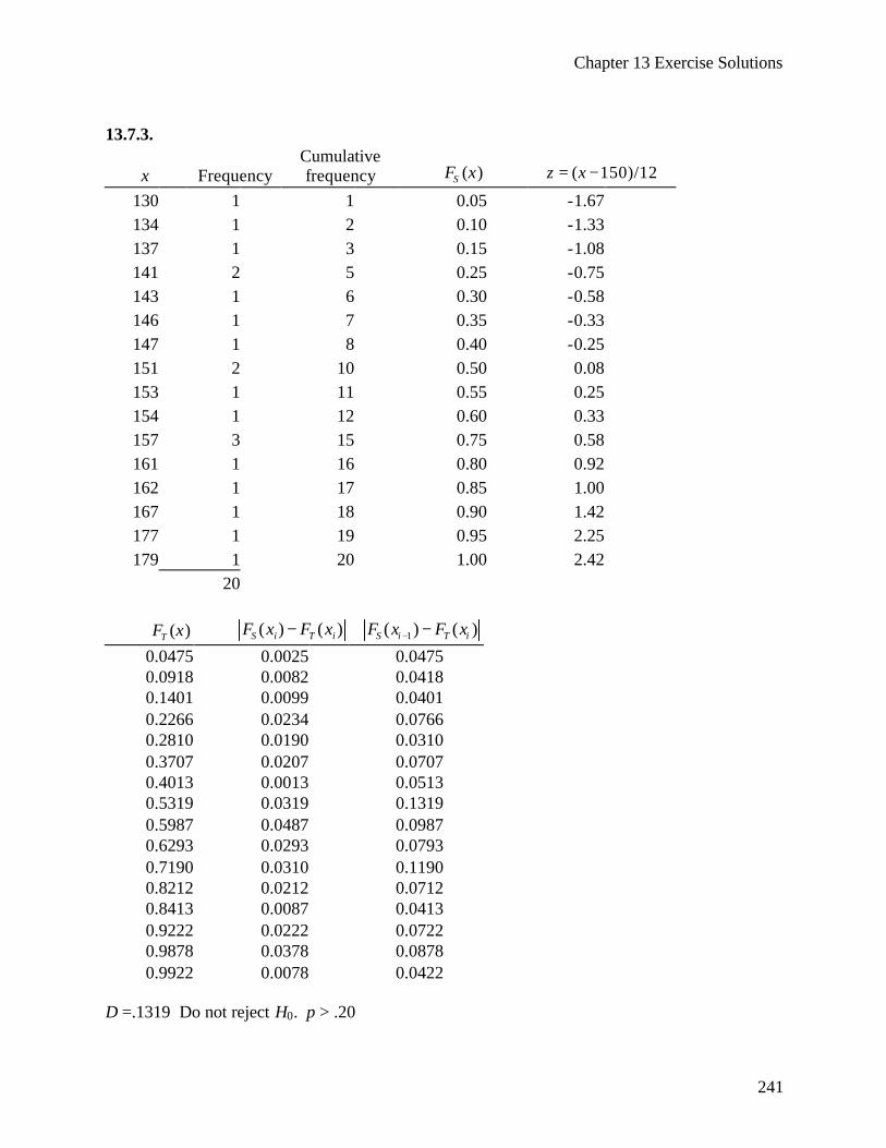
Chapter 13 Exercise Solutions
241
13.7.3.
x Frequency Cumulative frequency ( )SF x ( 150)/12z x= −
130 1 1 0.05 -1.67 134 1 2 0.10 -1.33 137 1 3 0.15 -1.08 141 2 5 0.25 -0.75 143 1 6 0.30 -0.58 146 1 7 0.35 -0.33 147 1 8 0.40 -0.25 151 2 10 0.50 0.08 153 1 11 0.55 0.25 154 1 12 0.60 0.33 157 3 15 0.75 0.58 161 1 16 0.80 0.92 162 1 17 0.85 1.00 167 1 18 0.90 1.42 177 1 19 0.95 2.25 179 1 20 1.00 2.42
20
( )TF x ( ) ( )S i T iF x F x− 1( ) ( )S i T iF x F x− −
0.0475 0.0025 0.0475 0.0918 0.0082 0.0418 0.1401 0.0099 0.0401 0.2266 0.0234 0.0766 0.2810 0.0190 0.0310 0.3707 0.0207 0.0707 0.4013 0.0013 0.0513 0.5319 0.0319 0.1319 0.5987 0.0487 0.0987 0.6293 0.0293 0.0793 0.7190 0.0310 0.1190 0.8212 0.0212 0.0712 0.8413 0.0087 0.0413 0.9222 0.0222 0.0722 0.9878 0.0378 0.0878 0.9922 0.0078 0.0422
D =.1319 Do not reject H0. p > .20
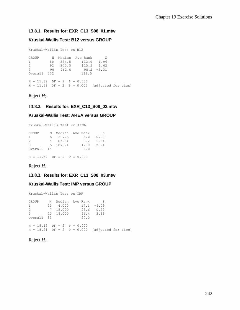
Chapter 13 Exercise Solutions
242
13.8.1. Results for: EXR_C13_S08_01.mtw Kruskal-Wallis Test: B12 versus GROUP Kruskal-Wallis Test on B12 GROUP N Median Ave Rank Z 1 50 334.5 133.0 1.96 2 92 345.0 125.5 1.65 3 90 262.0 98.2 -3.31 Overall 232 116.5 H = 11.38 DF = 2 P = 0.003 H = 11.38 DF = 2 P = 0.003 (adjusted for ties) Reject H0. 13.8.2. Results for: EXR_C13_S08_02.mtw Kruskal-Wallis Test: AREA versus GROUP Kruskal-Wallis Test on AREA GROUP N Median Ave Rank Z 1 5 80.75 8.0 0.00 2 5 63.24 3.2 -2.94 3 5 107.74 12.8 2.94 Overall 15 8.0 H = 11.52 DF = 2 P = 0.003 Reject H0. 13.8.3. Results for: EXR_C13_S08_03.mtw Kruskal-Wallis Test: IMP versus GROUP Kruskal-Wallis Test on IMP GROUP N Median Ave Rank Z 1 23 4.000 17.1 -4.09 2 7 15.000 28.6 0.29 3 23 18.000 36.4 3.89 Overall 53 27.0 H = 18.13 DF = 2 P = 0.000 H = 18.21 DF = 2 P = 0.000 (adjusted for ties) Reject H0.
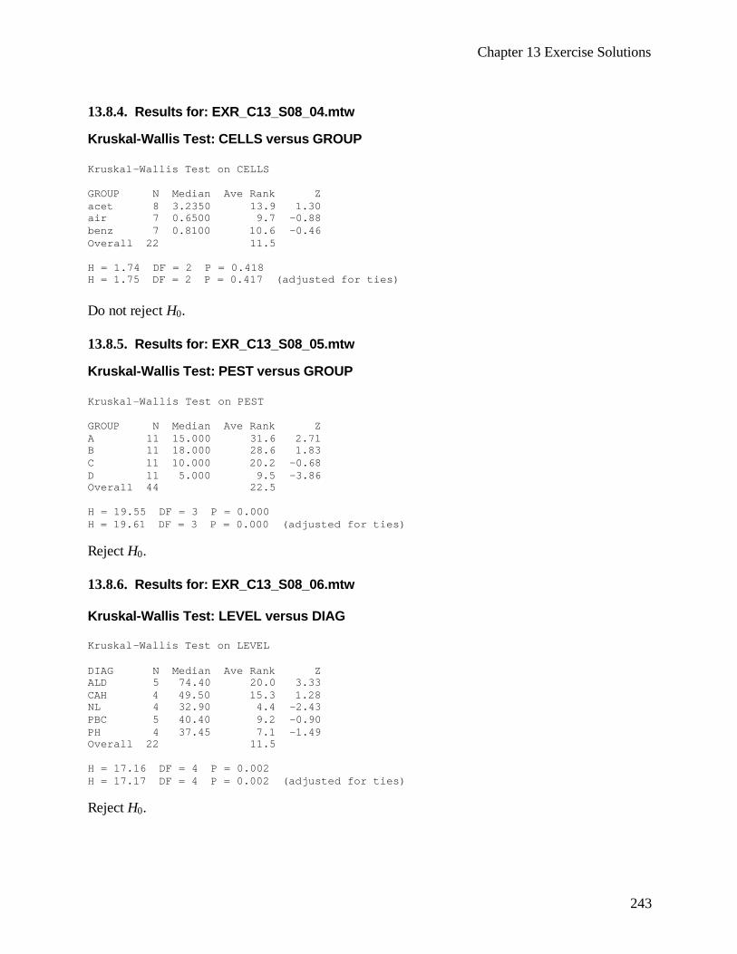
Chapter 13 Exercise Solutions
243
13.8.4. Results for: EXR_C13_S08_04.mtw Kruskal-Wallis Test: CELLS versus GROUP Kruskal-Wallis Test on CELLS GROUP N Median Ave Rank Z acet 8 3.2350 13.9 1.30 air 7 0.6500 9.7 -0.88 benz 7 0.8100 10.6 -0.46 Overall 22 11.5 H = 1.74 DF = 2 P = 0.418 H = 1.75 DF = 2 P = 0.417 (adjusted for ties) Do not reject H0. 13.8.5. Results for: EXR_C13_S08_05.mtw Kruskal-Wallis Test: PEST versus GROUP Kruskal-Wallis Test on PEST GROUP N Median Ave Rank Z A 11 15.000 31.6 2.71 B 11 18.000 28.6 1.83 C 11 10.000 20.2 -0.68 D 11 5.000 9.5 -3.86 Overall 44 22.5 H = 19.55 DF = 3 P = 0.000 H = 19.61 DF = 3 P = 0.000 (adjusted for ties) Reject H0. 13.8.6. Results for: EXR_C13_S08_06.mtw Kruskal-Wallis Test: LEVEL versus DIAG Kruskal-Wallis Test on LEVEL DIAG N Median Ave Rank Z ALD 5 74.40 20.0 3.33 CAH 4 49.50 15.3 1.28 NL 4 32.90 4.4 -2.43 PBC 5 40.40 9.2 -0.90 PH 4 37.45 7.1 -1.49 Overall 22 11.5 H = 17.16 DF = 4 P = 0.002 H = 17.17 DF = 4 P = 0.002 (adjusted for ties) Reject H0.
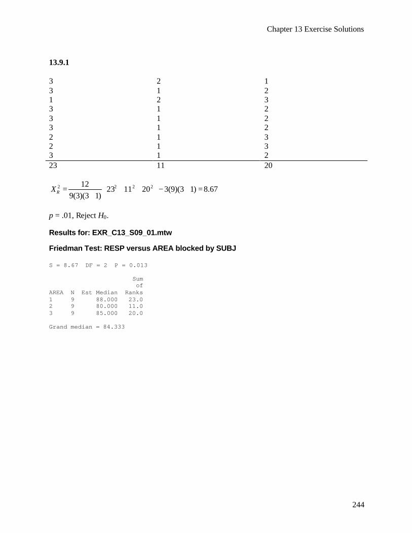
Chapter 13 Exercise Solutions
244
13.9.1 3 2 1 3 1 2 1 2 3 3 1 2 3 1 2 3 1 2 2 1 3 2 1 3 3 1 2 23 11 20
2 2 2 21223 11 20 3(9)(3 1) 8.67
9(3)(3 1)RX = + + − + = +
p = .01, Reject H0. Results for: EXR_C13_S09_01.mtw Friedman Test: RESP versus AREA blocked by SUBJ S = 8.67 DF = 2 P = 0.013 Sum of AREA N Est Median Ranks 1 9 88.000 23.0 2 9 80.000 11.0 3 9 85.000 20.0 Grand median = 84.333
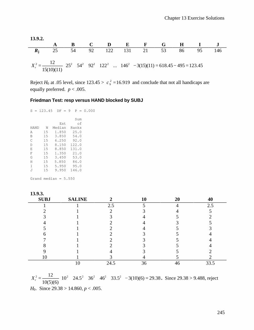
Chapter 13 Exercise Solutions
245
13.9.2.
A B C D E F G H I J Rj 25 54 92 122 131 21 53 86 95 146
2 2 2 2 2 212
25 54 92 122 ... 146 3(15)(11) 618.45 495 123.4515(10)(11)rX = + + + + + − = − =
Reject H0 at .05 level, since 123.45 > 2
9 16.919χ = and conclude that not all handicaps are equally preferred. p < .005. Friedman Test: resp versus HAND blocked by SUBJ S = 123.45 DF = 9 P = 0.000 Sum Est of HAND N Median Ranks A 15 1.850 25.0 B 15 3.850 54.0 C 15 6.250 92.0 D 15 8.150 122.0 E 15 8.850 131.0 F 15 1.350 21.0 G 15 3.450 53.0 H 15 5.850 86.0 I 15 5.950 95.0 J 15 9.950 146.0 Grand median = 5.550 13.9.3.
SUBJ SALINE 2 10 20 40 1 1 2.5 5 4 2.5 2 1 2 3 4 5 3 1 3 4 5 2 4 1 2 4 3 5 5 1 2 4 5 3 6 1 2 3 5 4 7 1 2 3 5 4 8 1 2 3 5 4 9 1 4 3 5 2 10 1 3 4 5 2 10 24.5 36 46 33.5
2 2 2 2 2 212
10 24.5 36 46 33.5 3(10)(6) 29.3810(5)(6)rX = + + + + − = . Since 29.38 > 9.488, reject
H0. Since 29.38 > 14.860, p < .005.

Chapter 13 Exercise Solutions
246
Friedman Test: RESP versus TREAT blocked by SUBJ S = 29.38 DF = 4 P = 0.000 S = 29.53 DF = 4 P = 0.000 (adjusted for ties) Sum of TREAT N Est Median Ranks SAL 10 -0.9815 10.0 T10 10 -0.2365 36.0 T2 10 -0.3395 24.5 T20 10 -0.1135 46.0 T40 10 -0.2865 33.5 Grand median = -0.3915 13.10.1.
di 2id
-2 4 -12 144
8 64 -11 121 -2 4 2 4
-2 4 -2 4 -2 4 9 81 1 1
-1 1 4 16
12 144 -2 4
600
2
6(600)1 .07, .20
15(15 1)Sr p= − = − >−
.
Do not reject H0.

Chapter 13 Exercise Solutions
247
13.10.2. di 2
id 7 49 6 36 3 9
-6 36 -6 36 -3 9 -9 81 -1 1 1 1 8 64 322
6(322)
1 .95, .00110(99)Sr p= − = − < .
Reject H0. 13.10.3.
di 2id
.00 .00 5.00 25.00
17.00 289.00 12.00 144.00 12.00 144.00 -1.00 1.00 2.00 4.00 6.00 36.00 7.50 56.25
-7.00 49.00 -4.00 16.00
-10.00 100.00 -2.50 6.25 -1.50 2.25 2.50 6.25
-4.00 16.00 .00 .00
-12.50 156.25 -8.50 72.25
-13.00 169.00 1292.5
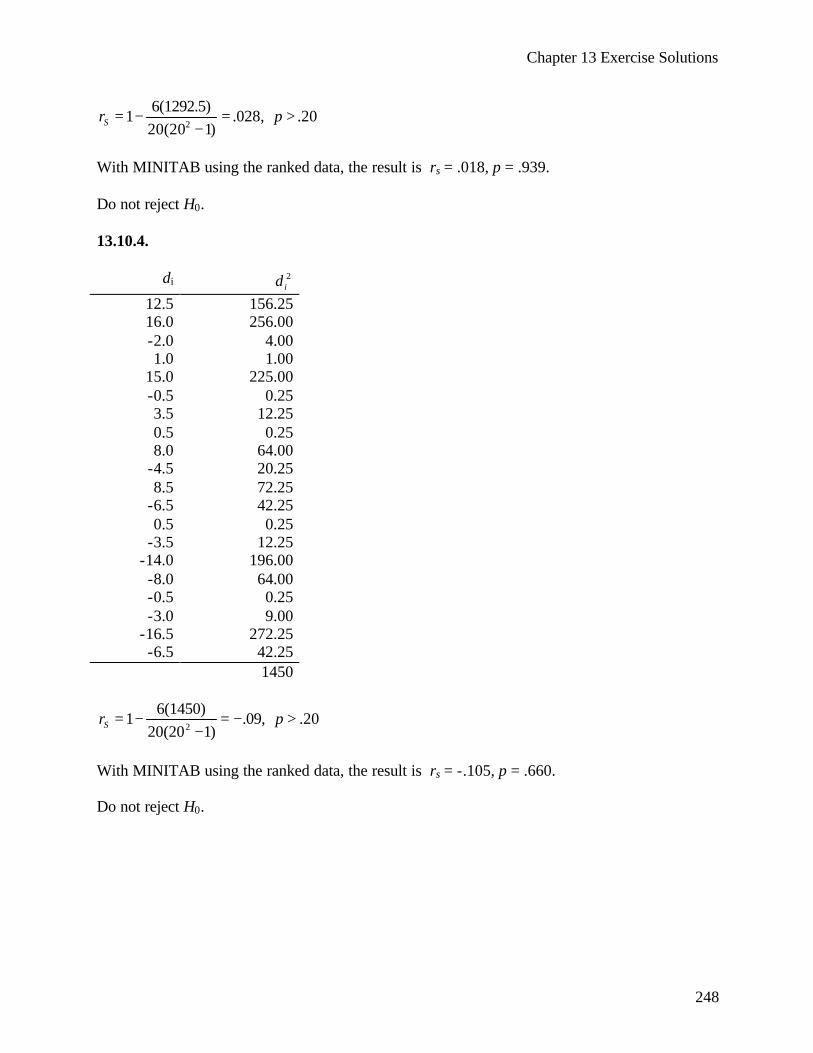
Chapter 13 Exercise Solutions
248
2
6(1292.5)1 .028, .20
20(20 1)Sr p= − = >−
With MINITAB using the ranked data, the result is rs = .018, p = .939. Do not reject H0. 13.10.4.
di 2id
12.5 156.25 16.0 256.00 -2.0 4.00 1.0 1.00
15.0 225.00 -0.5 0.25 3.5 12.25 0.5 0.25 8.0 64.00
-4.5 20.25 8.5 72.25
-6.5 42.25 0.5 0.25
-3.5 12.25 -14.0 196.00 -8.0 64.00 -0.5 0.25 -3.0 9.00
-16.5 272.25 -6.5 42.25
1450
2
6(1450)1 .09, .20
20(20 1)Sr p= − = − >−
With MINITAB using the ranked data, the result is rs = -.105, p = .660. Do not reject H0.
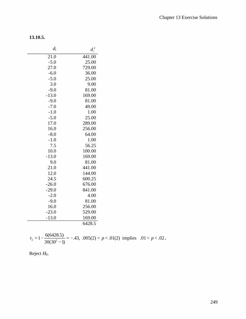
Chapter 13 Exercise Solutions
249
13.10.5.
di 2id
21.0 441.00 -5.0 25.00 27.0 729.00 -6.0 36.00 -5.0 25.00 3.0 9.00
-9.0 81.00 -13.0 169.00 -9.0 81.00 -7.0 49.00 -1.0 1.00 -5.0 25.00 17.0 289.00 16.0 256.00 -8.0 64.00 -1.0 1.00 7.5 56.25
10.0 100.00 -13.0 169.00
9.0 81.00 21.0 441.00 12.0 144.00 24.5 600.25
-26.0 676.00 -29.0 841.00 -2.0 4.00 -9.0 81.00 16.0 256.00
-23.0 529.00 -13.0 169.00
6428.5
2
6(6428.5)1 .43, .005(2) .01(2) implies .01 .02
30(30 1)Sr p p= − = − < < < <−
.
Reject H0.
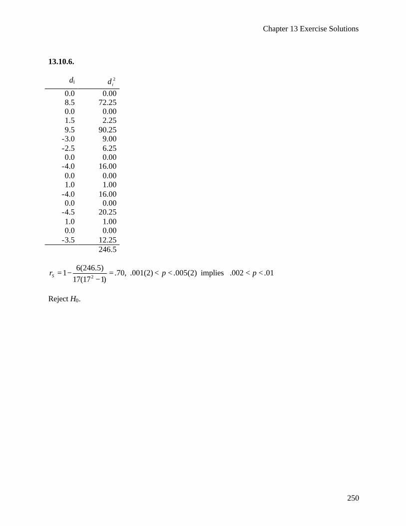
Chapter 13 Exercise Solutions
250
13.10.6.
di 2id
0.0 0.00 8.5 72.25 0.0 0.00 1.5 2.25 9.5 90.25
-3.0 9.00 -2.5 6.25 0.0 0.00
-4.0 16.00 0.0 0.00 1.0 1.00
-4.0 16.00 0.0 0.00
-4.5 20.25 1.0 1.00 0.0 0.00
-3.5 12.25 246.5
2
6(246.5)1 .70, .001(2) .005(2) implies .002 .01
17(17 1)Sr p p= − = < < < <−
Reject H0.
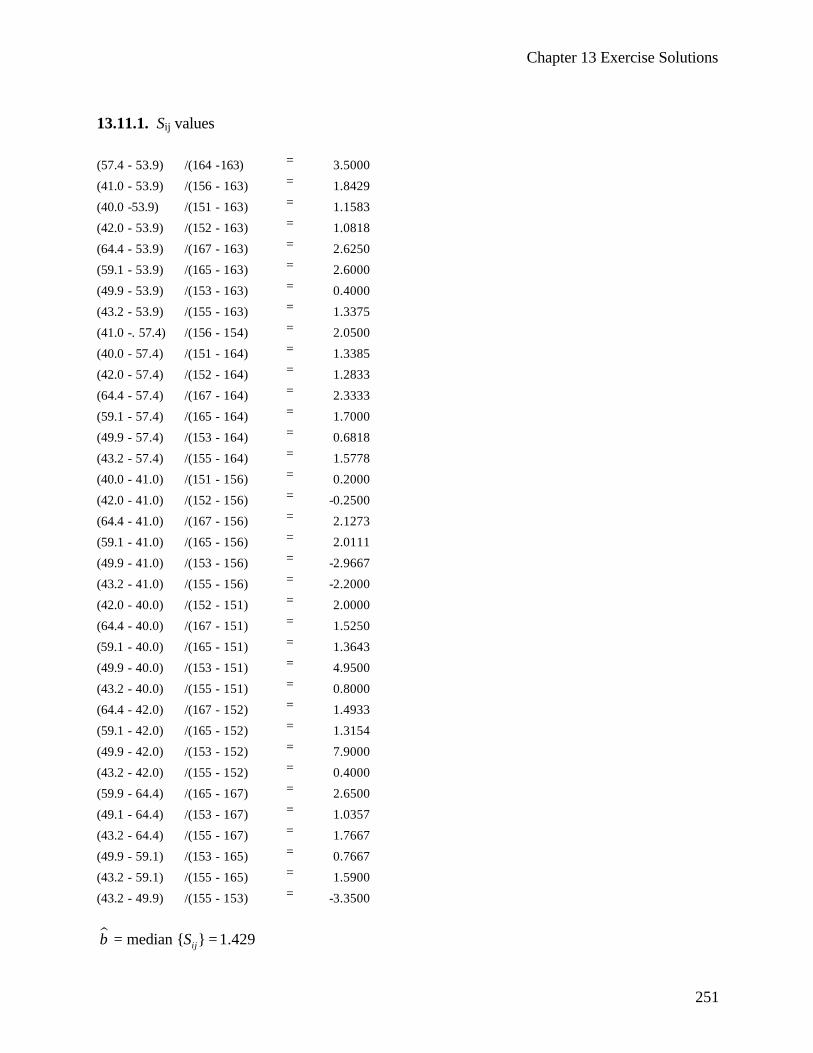
Chapter 13 Exercise Solutions
251
13.11.1. Sij values (57.4 - 53.9) /(164 -163) = 3.5000
(41.0 - 53.9) /(156 - 163) = 1.8429
(40.0 -53.9) /(151 - 163) = 1.1583
(42.0 - 53.9) /(152 - 163) = 1.0818
(64.4 - 53.9) /(167 - 163) = 2.6250
(59.1 - 53.9) /(165 - 163) = 2.6000
(49.9 - 53.9) /(153 - 163) = 0.4000
(43.2 - 53.9) /(155 - 163) = 1.3375
(41.0 -. 57.4) /(156 - 154) = 2.0500
(40.0 - 57.4) /(151 - 164) = 1.3385
(42.0 - 57.4) /(152 - 164) = 1.2833
(64.4 - 57.4) /(167 - 164) = 2.3333
(59.1 - 57.4) /(165 - 164) = 1.7000
(49.9 - 57.4) /(153 - 164) = 0.6818
(43.2 - 57.4) /(155 - 164) = 1.5778
(40.0 - 41.0) /(151 - 156) = 0.2000
(42.0 - 41.0) /(152 - 156) = -0.2500
(64.4 - 41.0) /(167 - 156) = 2.1273
(59.1 - 41.0) /(165 - 156) = 2.0111
(49.9 - 41.0) /(153 - 156) = -2.9667
(43.2 - 41.0) /(155 - 156) = -2.2000
(42.0 - 40.0) /(152 - 151) = 2.0000
(64.4 - 40.0) /(167 - 151) = 1.5250
(59.1 - 40.0) /(165 - 151) = 1.3643
(49.9 - 40.0) /(153 - 151) = 4.9500
(43.2 - 40.0) /(155 - 151) = 0.8000
(64.4 - 42.0) /(167 - 152) = 1.4933
(59.1 - 42.0) /(165 - 152) = 1.3154
(49.9 - 42.0) /(153 - 152) = 7.9000
(43.2 - 42.0) /(155 - 152) = 0.4000
(59.9 - 64.4) /(165 - 167) = 2.6500
(49.1 - 64.4) /(153 - 167) = 1.0357
(43.2 - 64.4) /(155 - 167) = 1.7667
(49.9 - 59.1) /(153 - 165) = 0.7667
(43.2 - 59.1) /(155 - 165) = 1.5900
(43.2 - 49.9) /(155 - 153) = -3.3500 µ median { } 1.429ijSβ = =
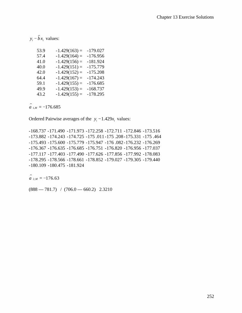
Chapter 13 Exercise Solutions
252
µ
i iy xβ− values:
53.9 -1.429(163) = -179.027 57.4 -1.429(164) = -176.956 41.0 -1.429(156) = -181.924 40.0 -1.429(151) = -175.779 42.0 -1.429(152) = -175.208 64.4 -1.429(167) = -174.243 59.1 -1.429(155) = -176.685 49.9 -1.429(153) = -168.737 43.2 -1.429(155) = -178.295
µ
1, 176.685Mα = − Ordered Pairwise averages of the 1.429i iy x− values: -168.737 -171.490 -171.973 -172.258 -172.711 -172.846 -173.516 -173.882 -174.243 -174.725 -175 .011 -175 .208 -175.331 -175 .464 -175.493 -175.600 -175.779 -175.947 -176 .082 -176.232 -176.269 -176.367 -176.635 -176.685 -176.751 -176.820 -176.956 -177.037 -177.117 -177.403 -177.490 -177.626 -177.856 -177.992 -178.083 -178.295 -178.566 -178.661 -178.852 -179.027 -179.305 -179.440 -180.109 -180.475 -181.924 µ
2, 176.63Mα = − (888 — 781.7) / (706.0 — 660.2) 2.3210
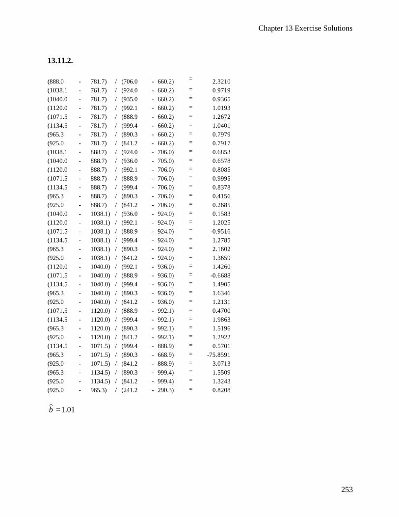
Chapter 13 Exercise Solutions
253
13.11.2. (888.0 - 781.7) / (706.0 - 660.2) = 2.3210 (1038.1 - 761.7) / (924.0 - 660.2) = 0.9719 (1040.0 - 781.7) / (935.0 - 660.2) = 0.9365 (1120.0 - 781.7) / (992.1 - 660.2) = 1.0193 (1071.5 - 781.7) / (888.9 - 660.2) = 1.2672 (1134.5 - 781.7) / (999.4 - 660.2) = 1.0401 (965.3 - 781.7) / (890.3 - 660.2) = 0.7979 (925.0 - 781.7) / (841.2 - 660.2) = 0.7917 (1038.1 - 888.7) / (924.0 - 706.0) = 0.6853 (1040.0 - 888.7) / (936.0 - 705.0) = 0.6578 (1120.0 - 888.7) / (992.1 - 706.0) = 0.8085 (1071.5 - 888.7) / (888.9 - 706.0) = 0.9995 (1134.5 - 888.7) / (999.4 - 706.0) = 0.8378 (965.3 - 888.7) / (890.3 - 706.0) = 0.4156 (925.0 - 888.7) / (841.2 - 706.0) = 0.2685 (1040.0 - 1038.1) / (936.0 - 924.0) = 0.1583 (1120.0 - 1038.1) / (992.1 - 924.0) = 1.2025 (1071.5 - 1038.1) / (888.9 - 924.0) = -0.9516 (1134.5 - 1038.1) / (999.4 - 924.0) = 1.2785 (965.3 - 1038.1) / (890.3 - 924.0) = 2.1602 (925.0 - 1038.1) / (641.2 - 924.0) = 1.3659 (1120.0 - 1040.0) / (992.1 - 936.0) = 1.4260 (1071.5 - 1040.0) / (888.9 - 936.0) = -0.6688 (1134.5 - 1040.0) / (999.4 - 936.0) = 1.4905 (965.3 - 1040.0) / (890.3 - 936.0) = 1.6346 (925.0 - 1040.0) / (841.2 - 936.0) = 1.2131 (1071.5 - 1120.0) / (888.9 - 992.1) = 0.4700 (1134.5 - 1120.0) / (999.4 - 992.1) = 1.9863 (965.3 - 1120.0) / (890.3 - 992.1) = 1.5196 (925.0 - 1120.0) / (841.2 - 992.1) = 1.2922 (1134.5 - 1071.5) / (999.4 - 888.9) = 0.5701 (965.3 - 1071.5) / (890.3 - 668.9) = -75.8591 (925.0 - 1071.5) / (841.2 - 888.9) = 3.0713 (965.3 - 1134.5) / (890.3 - 999.4) = 1.5509 (925.0 - 1134.5) / (841.2 - 999.4) = 1.3243 (925.0 - 965.3) / (241.2 - 290.3) = 0.8208 µ 1.01β =
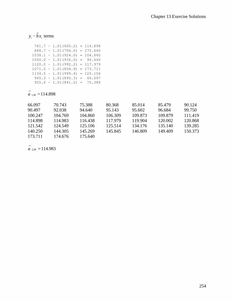
Chapter 13 Exercise Solutions
254
µi iy xβ− terms
781.7 – 1.01(660.2) = 114.898 888.7 – 1.01(706.0) = 275.640
1038.1 – 1.01(924.0) = 104.860 1040.0 – 1.01(936.0) = 94.640 1120.0 – 1.01(992.2) = 117.979 1071.5 – 1.01(858.9) = 173.711 1134.5 – 1.01(999.4) = 125.106 965.3 – 1.01(890.3) = 66.097 925.0 - 1.01(841.2) = 75.388
µ
1, 114.898Mα = 66.097 70.743 75.388 80.368 85.014 85.479 90.124 90.497 92.038 94.640 95.143 95.602 96.684 99.750 100.247 104.769 104.860 106.309 109.873 109.879 111.419 114.898 114.983 116.438 117.979 119.904 120.002 120.868 121.542 124.549 125.106 125.514 134.176 135.140 139.285 140.250 144.305 145.269 145.845 146.809 149.409 150.373 173.711 174.676 175.640 µ
2, 114.983Mα =
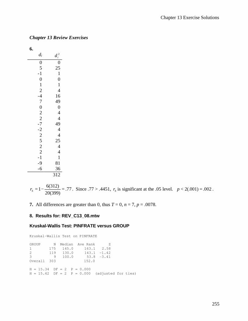
Chapter 13 Exercise Solutions
255
Chapter 13 Review Exercises 6.
di 2id
0 0 5 25
-1 1 0 0 1 1 2 4
-4 16 7 49 0 0 2 4 2 4
-7 49 -2 4 2 4 5 25 2 4 2 4
-1 1 -9 81 -6 36
312
6(312)1 .77
20(399)Sr = − = . Since .77 > .4451, Sr is significant at the .05 level. 2(.001) .002p < = .
7. All differences are greater than 0, thus T = 0, n = 7, p = .0078. 8. Results for: REV_C13_08.mtw Kruskal-Wallis Test: PINFRATE versus GROUP Kruskal-Wallis Test on PINFRATE GROUP N Median Ave Rank Z 1 175 145.0 163.1 2.58 2 119 130.0 143.1 -1.42 3 9 100.0 53.8 -3.41 Overall 303 152.0 H = 15.34 DF = 2 P = 0.000 H = 15.42 DF = 2 P = 0.000 (adjusted for ties)
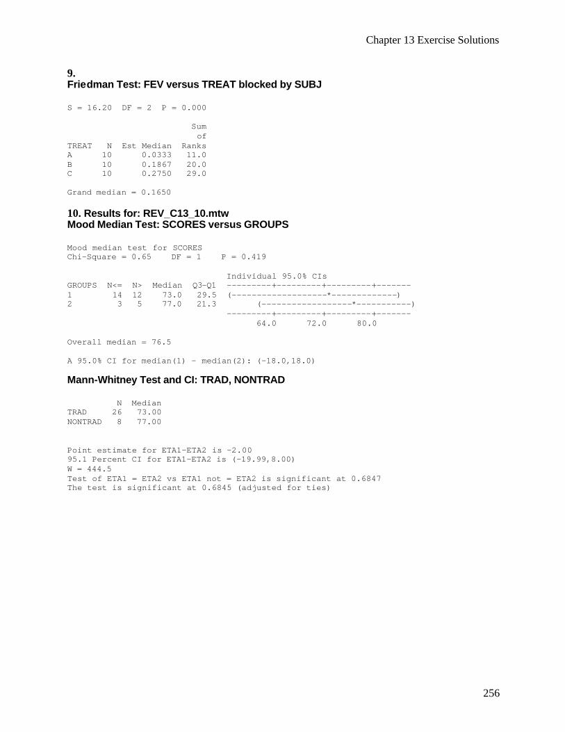
Chapter 13 Exercise Solutions
256
9. Friedman Test: FEV versus TREAT blocked by SUBJ S = 16.20 DF = 2 P = 0.000 Sum of TREAT N Est Median Ranks A 10 0.0333 11.0 B 10 0.1867 20.0 C 10 0.2750 29.0 Grand median = 0.1650 10. Results for: REV_C13_10.mtw Mood Median Test: SCORES versus GROUPS Mood median test for SCORES Chi-Square = 0.65 DF = 1 P = 0.419 Individual 95.0% CIs GROUPS N<= N> Median Q3-Q1 ---------+---------+---------+------- 1 14 12 73.0 29.5 (-------------------*-------------) 2 3 5 77.0 21.3 (------------------*-----------) ---------+---------+---------+------- 64.0 72.0 80.0 Overall median = 76.5 A 95.0% CI for median(1) - median(2): (-18.0,18.0) Mann-Whitney Test and CI: TRAD, NONTRAD N Median TRAD 26 73.00 NONTRAD 8 77.00 Point estimate for ETA1-ETA2 is -2.00 95.1 Percent CI for ETA1-ETA2 is (-19.99,8.00) W = 444.5 Test of ETA1 = ETA2 vs ETA1 not = ETA2 is significant at 0.6847 The test is significant at 0.6845 (adjusted for ties)
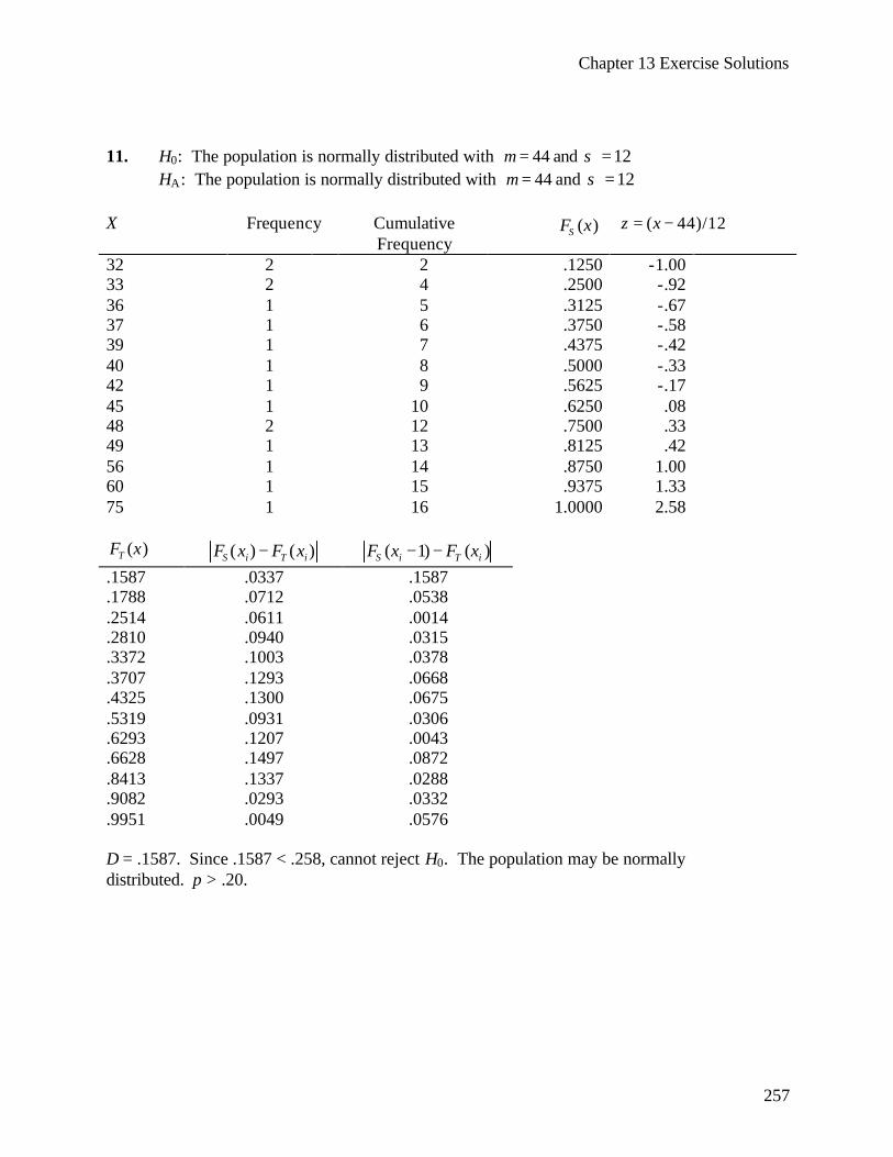
Chapter 13 Exercise Solutions
257
11. H0: The population is normally distributed with 44µ = and 12σ = HA: The population is normally distributed with 44µ = and 12σ = X Frequency Cumulative
Frequency ( )SF x ( 44)/12z x= −
32 2 2 .1250 -1.00 33 2 4 .2500 -.92 36 1 5 .3125 -.67 37 1 6 .3750 -.58 39 1 7 .4375 -.42 40 1 8 .5000 -.33 42 1 9 .5625 -.17 45 1 10 .6250 .08 48 2 12 .7500 .33 49 1 13 .8125 .42 56 1 14 .8750 1.00 60 1 15 .9375 1.33 75 1 16 1.0000 2.58
( )TF x ( ) ( )S i T iF x F x− ( 1) ( )S i T iF x F x− − .1587 .0337 .1587 .1788 .0712 .0538 .2514 .0611 .0014 .2810 .0940 .0315 .3372 .1003 .0378 .3707 .1293 .0668 .4325 .1300 .0675 .5319 .0931 .0306 .6293 .1207 .0043 .6628 .1497 .0872 .8413 .1337 .0288 .9082 .0293 .0332 .9951 .0049 .0576 D = .1587. Since .1587 < .258, cannot reject H0. The population may be normally distributed. p > .20.
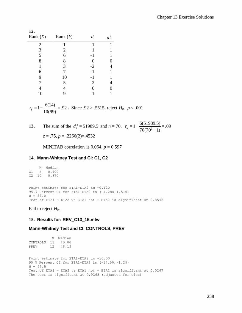
Chapter 13 Exercise Solutions
258
12. Rank (X) Rank (Y) di 2
id 2 1 1 1 3 2 1 1 5 6 -1 1 8 8 0 0 1 3 -2 4 6 7 -1 1 9 10 -1 1 7 5 2 4 4 4 0 0 10 9 1 1
6(14)
1 .9210(99)Sr = − = . Since .92 > .5515, reject H0. p < .001
13. The sum of the 2 51989.5id = and n = 70. 2
6(51989.5)1 .09
70(70 1)Sr = − =−
z = .75, p = .2266(2)=.4532 MINITAB correlation is 0.064, p = 0.597
14. Mann-Whitney Test and CI: C1, C2 N Median C1 5 0.900 C2 10 0.870 Point estimate for ETA1-ETA2 is -0.120 95.7 Percent CI for ETA1-ETA2 is (-1.280,1.510) W = 38.0 Test of ETA1 = ETA2 vs ETA1 not = ETA2 is significant at 0.8542 Fail to reject H0. 15. Results for: REV_C13_15.mtw Mann-Whitney Test and CI: CONTROLS, PREV N Median CONTROLS 11 40.00 PREV 12 48.13 Point estimate for ETA1-ETA2 is -10.00 95.5 Percent CI for ETA1-ETA2 is (-17.50,-1.25) W = 95.5 Test of ETA1 = ETA2 vs ETA1 not = ETA2 is significant at 0.0267 The test is significant at 0.0263 (adjusted for ties)
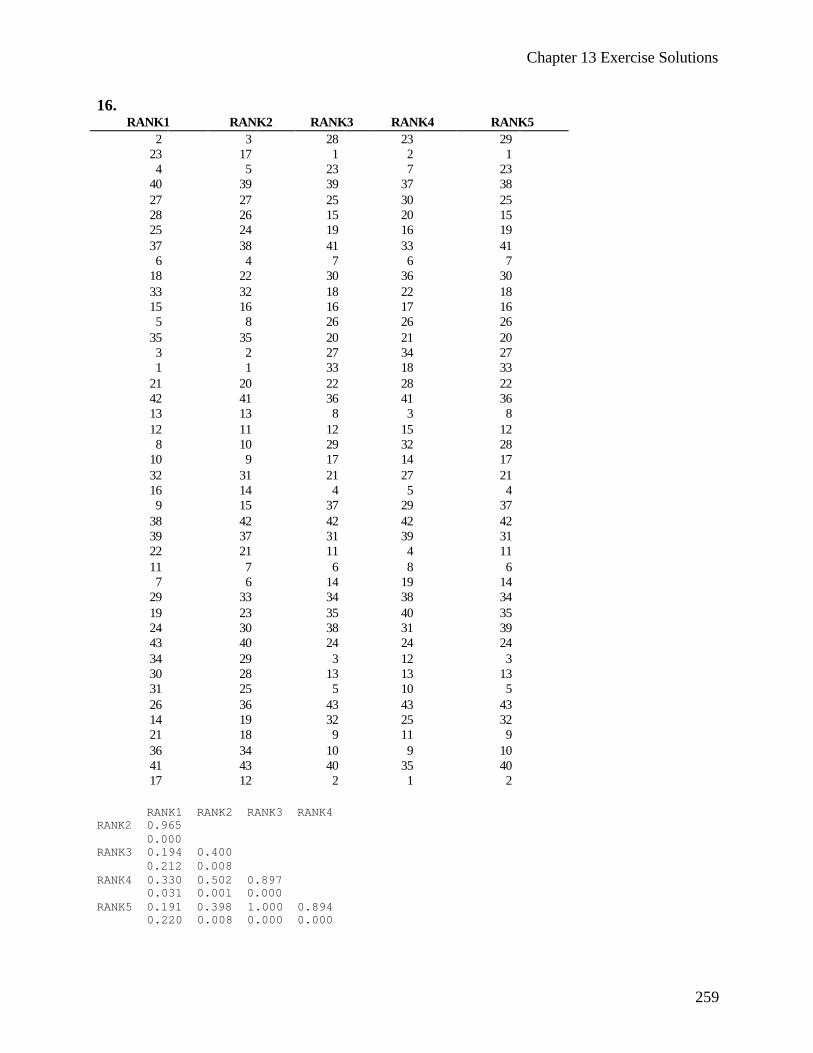
Chapter 13 Exercise Solutions
259
16. RANK1 RANK2 RANK3 RANK4 RANK5
2 3 28 23 29 23 17 1 2 1 4 5 23 7 23
40 39 39 37 38 27 27 25 30 25 28 26 15 20 15 25 24 19 16 19 37 38 41 33 41 6 4 7 6 7
18 22 30 36 30 33 32 18 22 18 15 16 16 17 16 5 8 26 26 26
35 35 20 21 20 3 2 27 34 27 1 1 33 18 33
21 20 22 28 22 42 41 36 41 36 13 13 8 3 8 12 11 12 15 12 8 10 29 32 28
10 9 17 14 17 32 31 21 27 21 16 14 4 5 4 9 15 37 29 37
38 42 42 42 42 39 37 31 39 31 22 21 11 4 11 11 7 6 8 6 7 6 14 19 14
29 33 34 38 34 19 23 35 40 35 24 30 38 31 39 43 40 24 24 24 34 29 3 12 3 30 28 13 13 13 31 25 5 10 5 26 36 43 43 43 14 19 32 25 32 21 18 9 11 9 36 34 10 9 10 41 43 40 35 40 17 12 2 1 2
RANK1 RANK2 RANK3 RANK4 RANK2 0.965 0.000 RANK3 0.194 0.400 0.212 0.008 RANK4 0.330 0.502 0.897 0.031 0.001 0.000 RANK5 0.191 0.398 1.000 0.894 0.220 0.008 0.000 0.000
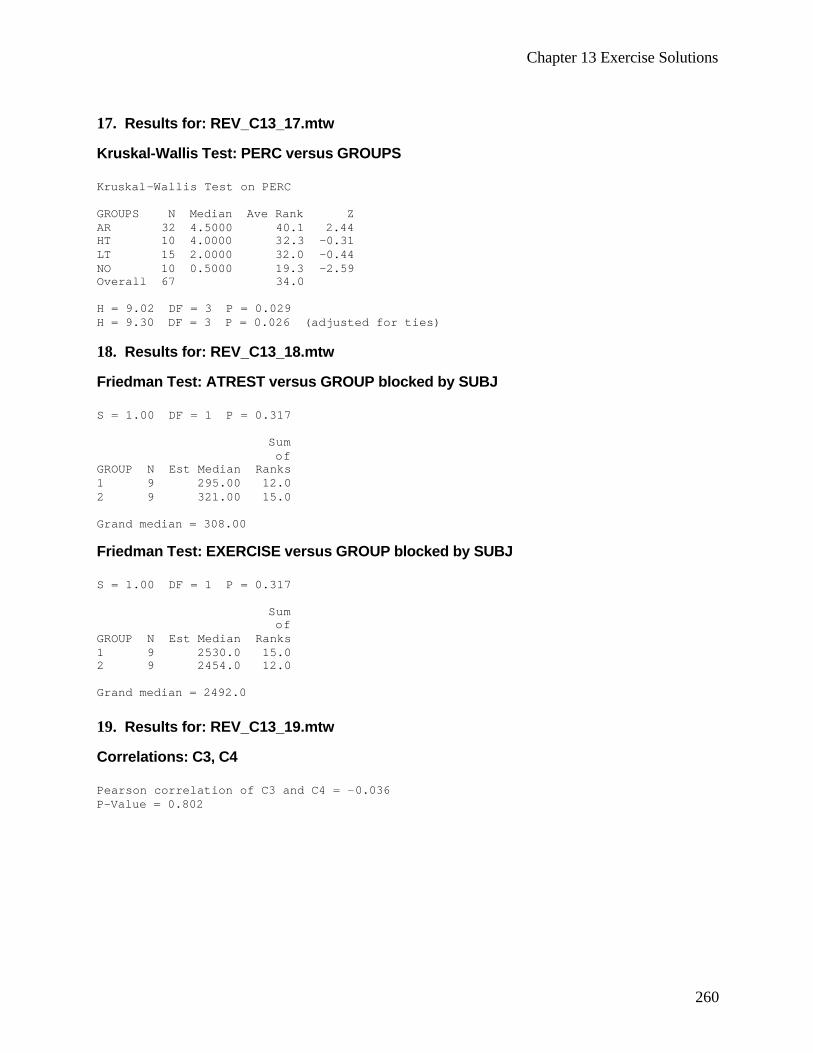
Chapter 13 Exercise Solutions
260
17. Results for: REV_C13_17.mtw Kruskal-Wallis Test: PERC versus GROUPS Kruskal-Wallis Test on PERC GROUPS N Median Ave Rank Z AR 32 4.5000 40.1 2.44 HT 10 4.0000 32.3 -0.31 LT 15 2.0000 32.0 -0.44 NO 10 0.5000 19.3 -2.59 Overall 67 34.0 H = 9.02 DF = 3 P = 0.029 H = 9.30 DF = 3 P = 0.026 (adjusted for ties) 18. Results for: REV_C13_18.mtw Friedman Test: ATREST versus GROUP blocked by SUBJ S = 1.00 DF = 1 P = 0.317 Sum of GROUP N Est Median Ranks 1 9 295.00 12.0 2 9 321.00 15.0 Grand median = 308.00 Friedman Test: EXERCISE versus GROUP blocked by SUBJ S = 1.00 DF = 1 P = 0.317 Sum of GROUP N Est Median Ranks 1 9 2530.0 15.0 2 9 2454.0 12.0 Grand median = 2492.0 19. Results for: REV_C13_19.mtw Correlations: C3, C4 Pearson correlation of C3 and C4 = -0.036 P-Value = 0.802

Chapter 13 Exercise Solutions
261
20. Control Subjects Only after taking DIFF = POST - PRE Wilcoxon Signed Rank CI: DIFF Confidence Estimated Achieved Interval N Median Confidence Lower Upper DIFF 16 24.8 94.8 4.3 41.0 Wilcoxon Signed Rank Test: DIFF Test of median = 0.000000 versus median not = 0.000000 N for Wilcoxon Estimated N Test Statistic P Median DIFF 16 16 126.0 0.003 24.78 Patient Subjects Only after taking DIFF = POST - PRE Wilcoxon Signed Rank CI: DIFF Confidence Estimated Achieved Interval N Median Confidence Lower Upper DIFF 15 28.7 95.0 15.3 59.9 MTB > WTest 0.0 'DIFF'; SUBC> Alternative 0. Wilcoxon Signed Rank Test: DIFF Test of median = 0.000000 versus median not = 0.000000 N for Wilcoxon Estimated N Test Statistic P Median DIFF 15 15 120.0 0.001 28.74 21. Mann-Whitney Test and CI: T41, T42 N Median T41 9 50.00 T42 34 81.50 Point estimate for ETA1-ETA2 is -34.00 95.3 Percent CI for ETA1-ETA2 is (-64.00,-8.99) W = 107.5 Test of ETA1 = ETA2 vs ETA1 not = ETA2 is significant at 0.0072 The test is significant at 0.0072 (adjusted for ties)
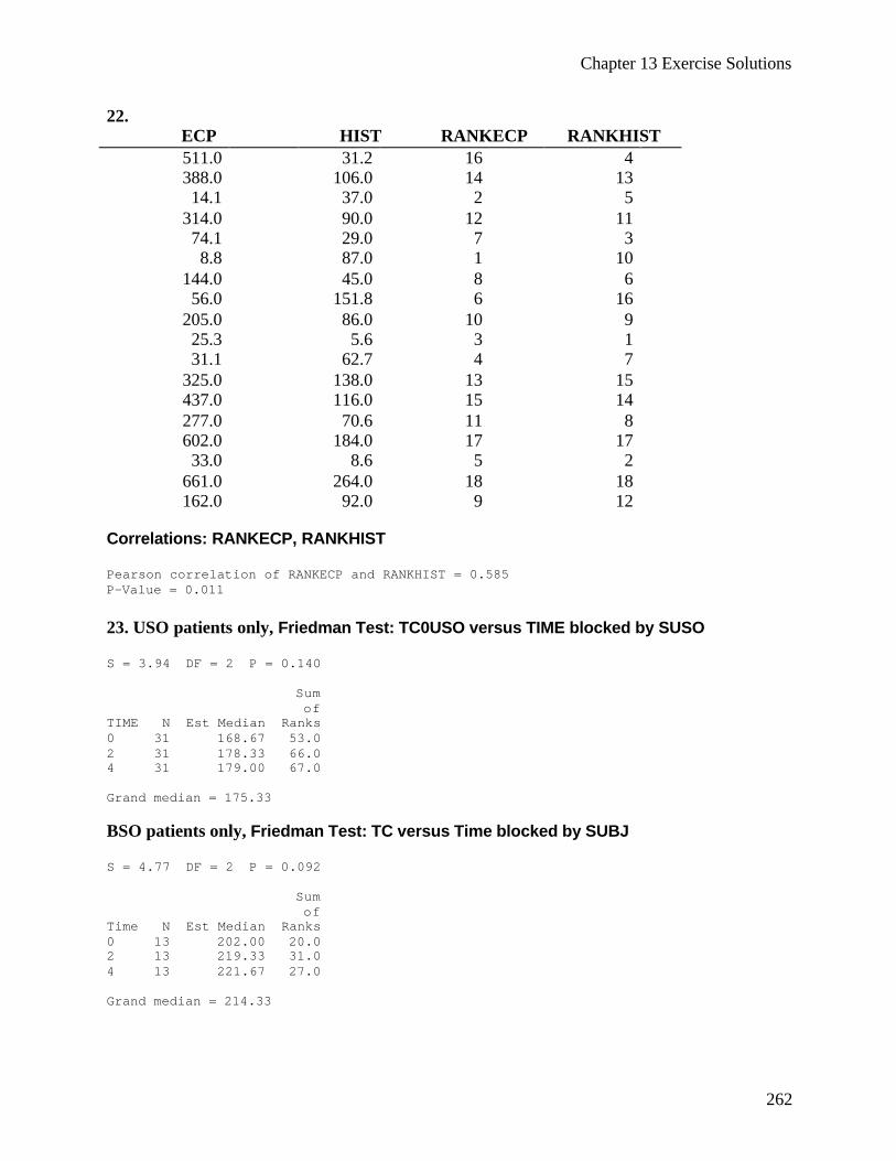
Chapter 13 Exercise Solutions
262
22. ECP HIST RANKECP RANKHIST 511.0 31.2 16 4 388.0 106.0 14 13 14.1 37.0 2 5
314.0 90.0 12 11 74.1 29.0 7 3 8.8 87.0 1 10
144.0 45.0 8 6 56.0 151.8 6 16
205.0 86.0 10 9 25.3 5.6 3 1 31.1 62.7 4 7
325.0 138.0 13 15 437.0 116.0 15 14 277.0 70.6 11 8 602.0 184.0 17 17 33.0 8.6 5 2
661.0 264.0 18 18 162.0 92.0 9 12
Correlations: RANKECP, RANKHIST Pearson correlation of RANKECP and RANKHIST = 0.585 P-Value = 0.011 23. USO patients only, Friedman Test: TC0USO versus TIME blocked by SUSO S = 3.94 DF = 2 P = 0.140 Sum of TIME N Est Median Ranks 0 31 168.67 53.0 2 31 178.33 66.0 4 31 179.00 67.0 Grand median = 175.33 BSO patients only, Friedman Test: TC versus Time blocked by SUBJ S = 4.77 DF = 2 P = 0.092 Sum of Time N Est Median Ranks 0 13 202.00 20.0 2 13 219.33 31.0 4 13 221.67 27.0 Grand median = 214.33
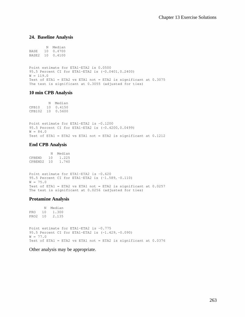
Chapter 13 Exercise Solutions
263
24. Baseline Analysis N Median BASE 10 0.4700 BASE2 10 0.4100 Point estimate for ETA1-ETA2 is 0.0500 95.5 Percent CI for ETA1-ETA2 is (-0.0401,0.2400) W = 119.0 Test of ETA1 = ETA2 vs ETA1 not = ETA2 is significant at 0.3075 The test is significant at 0.3055 (adjusted for ties) 10 min CPB Analysis N Median CPB10 10 0.4150 CPB102 10 0.5600 Point estimate for ETA1-ETA2 is -0.1200 95.5 Percent CI for ETA1-ETA2 is (-0.4200,0.0499) W = 84.0 Test of ETA1 = ETA2 vs ETA1 not = ETA2 is significant at 0.1212 End CPB Analysis N Median CPBEND 10 1.225 CPBEND2 10 1.740 Point estimate for ETA1-ETA2 is -0.620 95.5 Percent CI for ETA1-ETA2 is (-1.589,-0.110) W = 75.0 Test of ETA1 = ETA2 vs ETA1 not = ETA2 is significant at 0.0257 The test is significant at 0.0256 (adjusted for ties) Protamine Analysis N Median PRO 10 1.300 PRO2 10 2.135 Point estimate for ETA1-ETA2 is -0.775 95.5 Percent CI for ETA1-ETA2 is (-1.429,-0.090) W = 77.0 Test of ETA1 = ETA2 vs ETA1 not = ETA2 is significant at 0.0376 Other analysis may be appropriate.
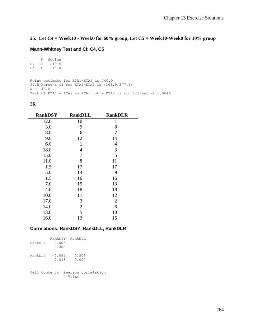
Chapter 13 Exercise Solutions
264
25. Let C4 = Week10 - Week0 for 60% group, Let C5 = Week10-Week0 for 10% group Mann-Whitney Test and CI: C4, C5 N Median C4 10 219.5 C5 10 -43.0 Point estimate for ETA1-ETA2 is 240.0 95.5 Percent CI for ETA1-ETA2 is (108.9,377.9) W = 143.0 Test of ETA1 = ETA2 vs ETA1 not = ETA2 is significant at 0.0046 26.
RankDSY RankDLL RankDLR 12.0 10 1 3.0 9 8 8.0 6 7 9.0 12 14 6.0 1 4
18.0 4 3 15.0 7 5 11.0 8 11 1.5 17 17 5.0 14 9 1.5 16 16 7.0 15 13 4.0 18 18
10.0 11 12 17.0 3 2 14.0 2 6 13.0 5 10 16.0 13 15
Correlations: RankDSY, RankDLL, RankDLR RankDSY RankDLL RankDLL -0.603 0.008 RankDLR -0.551 0.808 0.018 0.000 Cell Contents: Pearson correlation P-Value

Chapter 13 Exercise Solutions
265
27. Mann-Whitney Test and CI: PFKC, PFKCOPD N Median PFKC 9 51.60 PFKCOPD 9 61.30 Point estimate for ETA1-ETA2 is -1.60 95.8 Percent CI for ETA1-ETA2 is (-33.58,38.29) W = 83.0 Test of ETA1 = ETA2 vs ETA1 not = ETA2 is significant at 0.8598 Mann-Whitney Test and CI: HKC, HKCOPD N Median HKC 9 2.400 HKCOPD 9 1.600 Point estimate for ETA1-ETA2 is 0.800 95.8 Percent CI for ETA1-ETA2 is (-0.100,1.201) W = 106.5 Test of ETA1 = ETA2 vs ETA1 not = ETA2 is significant at 0.0703 The test is significant at 0.0695 (adjusted for ties) Mann-Whitney Test and CI: LDHC, LDHCOPD N Median LDHC 9 216.8 LDHCOPD 9 204.7 Point estimate for ETA1-ETA2 is -6.5 95.8 Percent CI for ETA1-ETA2 is (-142.2,92.3) W = 82.0 Test of ETA1 = ETA2 vs ETA1 not = ETA2 is significant at 0.7911 28. Results for: REV_C13_28.mtw Kruskal-Wallis Test: SERUM versus GROUPS Kruskal-Wallis Test on SERUM GROUPS N Median Ave Rank Z 1 10 0.2510 9.6 -2.73 2 14 0.5690 19.4 1.87 3 7 0.3350 18.5 0.83 Overall 31 16.0 H = 7.47 DF = 2 P = 0.024 H = 7.58 DF = 2 P = 0.023 (adjusted for ties)
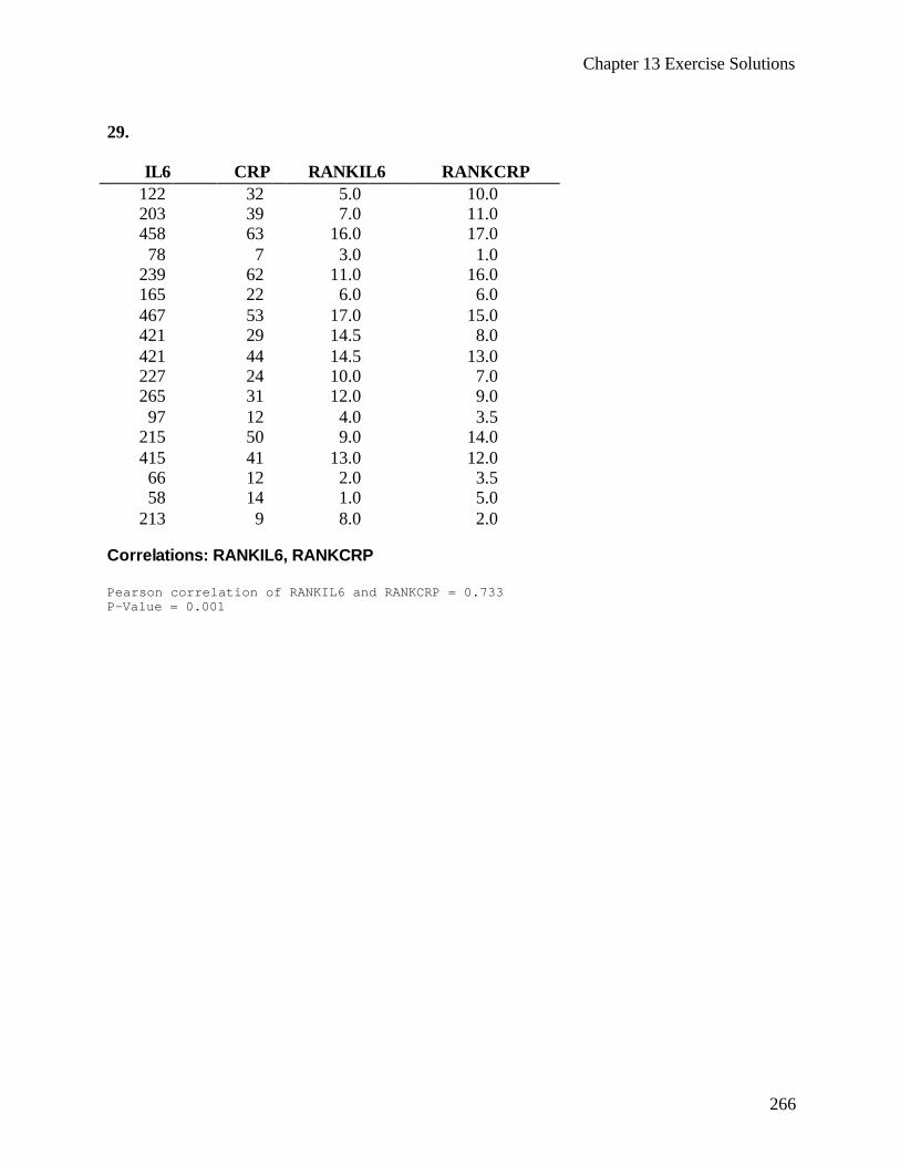
Chapter 13 Exercise Solutions
266
29.
IL6 CRP RANKIL6 RANKCRP 122 32 5.0 10.0 203 39 7.0 11.0 458 63 16.0 17.0 78 7 3.0 1.0
239 62 11.0 16.0 165 22 6.0 6.0 467 53 17.0 15.0 421 29 14.5 8.0 421 44 14.5 13.0 227 24 10.0 7.0 265 31 12.0 9.0 97 12 4.0 3.5
215 50 9.0 14.0 415 41 13.0 12.0 66 12 2.0 3.5 58 14 1.0 5.0
213 9 8.0 2.0 Correlations: RANKIL6, RANKCRP Pearson correlation of RANKIL6 and RANKCRP = 0.733 P-Value = 0.001

Chapter 14 Exercise Solutions
267
Chapter 14
14.2.1. (a) 1366
*1000 5.8236517
=
(b) White: 898
*1000 10.089741
= , Black: 446
*1000 3.7121927
=
(c) 41
*1000 9.434350
= (d) 24
*1000 5.54350
= (e) 41
*1000 9.434350
=
(f) MN303
*100 22.21366
= , MCD 471
*100 34.51366
=
14.2.2.
Age (years) Population Deaths
Age-Specific Death Rates
(per 100,000) Population Standard
Population
No. of Expected
Deaths 0-4 580,222 1,197 206.3003471 19,175,798 68138.96712 140.570926 5-9 577,151 126 21.83137515 20,549,505 73020.27512 15.9413302
10-14 563,293 153 27.16170803 20,528,072 72944.11544 19.8128677 15-19 570,547 460 80.62438327 20,219,890 71849.02656 57.9278346 20-44 3,083,521 4,989 161.7955577 104,004,252 369567.0088 597.943003 45-64 1,653,515 12,633 764.0087934 61,952,636 220141.4839 1681.9003
65 and over 761,457 42,076 5525.722398 34,991,753 124339.1231 6870.63477 Total 7,789,706 61,634 281,421,906 1000000 9384.73103
Age-adjusted death rate = 9384.73
*1000 9.41,000,000
=
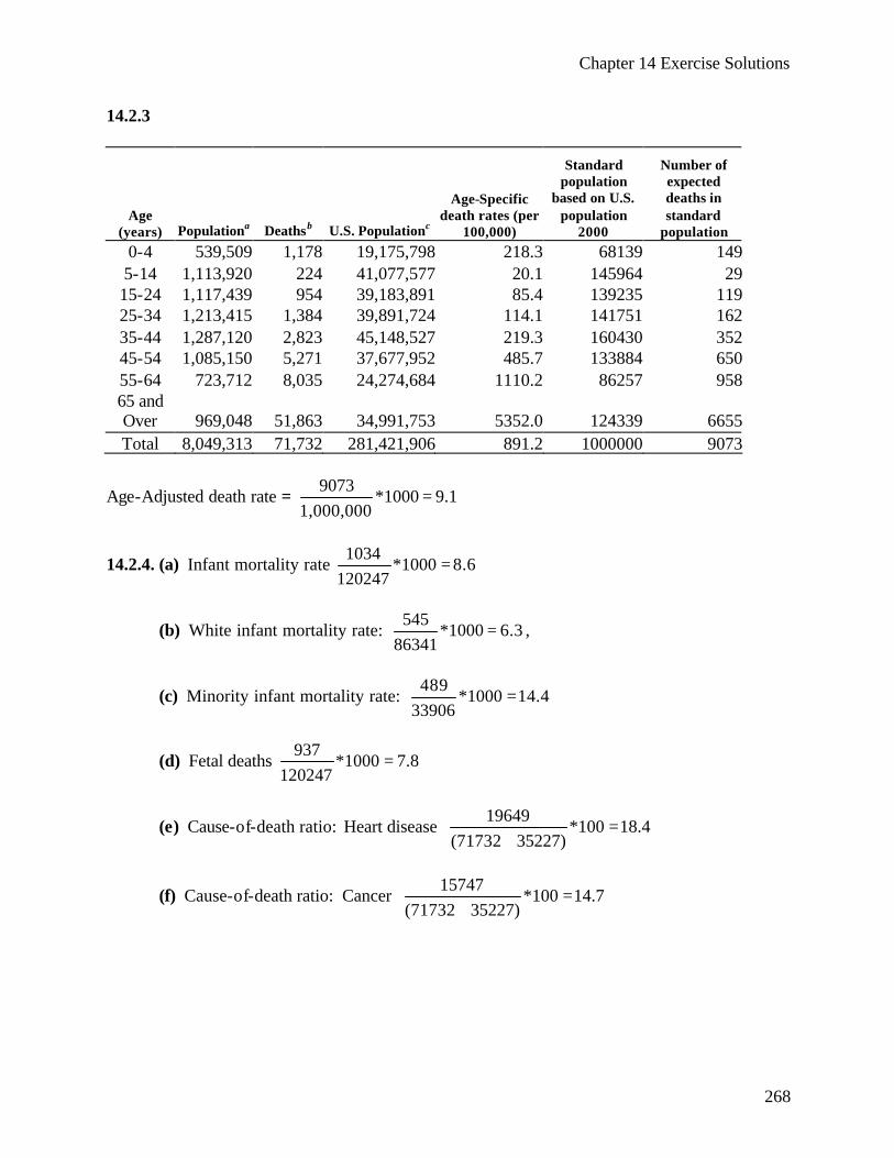
Chapter 14 Exercise Solutions
268
14.2.3
Age (years) Populationa Deathsb U.S. Populationc
Age-Specific death rates (per
100,000)
Standard population
based on U.S. population
2000
Number of expected deaths in standard
population 0-4 539,509 1,178 19,175,798 218.3 68139 1495-14 1,113,920 224 41,077,577 20.1 145964 2915-24 1,117,439 954 39,183,891 85.4 139235 11925-34 1,213,415 1,384 39,891,724 114.1 141751 16235-44 1,287,120 2,823 45,148,527 219.3 160430 35245-54 1,085,150 5,271 37,677,952 485.7 133884 65055-64 723,712 8,035 24,274,684 1110.2 86257 95865 and Over 969,048 51,863 34,991,753 5352.0 124339 6655Total 8,049,313 71,732 281,421,906 891.2 1000000 9073
Age-Adjusted death rate = 9073
*1000 9.11,000,000
=
14.2.4. (a) Infant mortality rate 1034
*1000 8.6120247
=
(b) White infant mortality rate: 545
*1000 6.386341
= ,
(c) Minority infant mortality rate: 489
*1000 14.433906
=
(d) Fetal deaths 937
*1000 7.8120247
=
(e) Cause-of-death ratio: Heart disease 19649
*100 18.4(71732 35227)
=+
(f) Cause-of-death ratio: Cancer 15747
*100 14.7(71732 35227)
=+
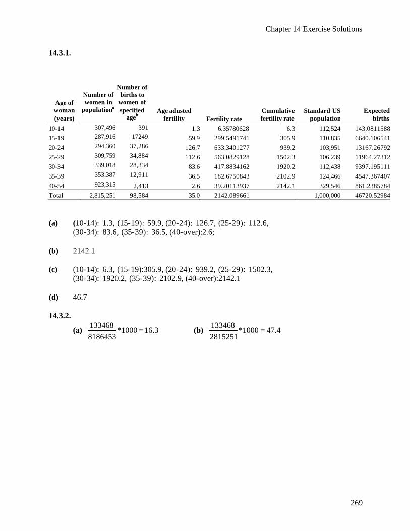
Chapter 14 Exercise Solutions
269
14.3.1.
Age of woman (years)
Number of women in
populationa
Number of births to
women of specified
ageb Age adusted
fertility Fertility rate Cumulative fertility rate
Standard US population
Expected births
10-14 307,496 391 1.3 6.35780628 6.3 112,524 143.0811588 15-19 287,916 17249 59.9 299.5491741 305.9 110,835 6640.106541 20-24 294,360 37,286 126.7 633.3401277 939.2 103,951 13167.26792 25-29 309,759 34,884 112.6 563.0829128 1502.3 106,239 11964.27312 30-34 339,018 28,334 83.6 417.8834162 1920.2 112,438 9397.195111 35-39 353,387 12,911 36.5 182.6750843 2102.9 124,466 4547.367407 40-54 923,315 2,413 2.6 39.20113937 2142.1 329,546 861.2385784 Total 2,815,251 98,584 35.0 2142.089661 1,000,000 46720.52984 (a) (10-14): 1.3, (15-19): 59.9, (20-24): 126.7, (25-29): 112.6,
(30-34): 83.6, (35-39): 36.5, (40-over):2.6; (b) 2142.1 (c) (10-14): 6.3, (15-19):305.9, (20-24): 939.2, (25-29): 1502.3,
(30-34): 1920.2, (35-39): 2102.9, (40-over):2142.1 (d) 46.7 14.3.2.
(a) 133468
*1000 16.38186453
= (b) 133468
*1000 47.42815251
=
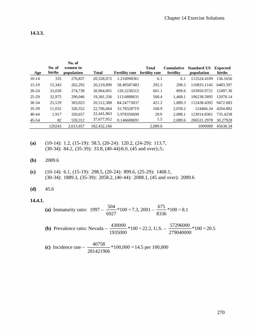
Chapter 14 Exercise Solutions
270
14.3.3.
Age No. of births
No. of women in population Total Fertility rate
Total fertility rate
Cumulative fertility
Standard US population
Expected births
10-14 335 276,837 20,528,072 1.210098361 6.1 6.1 112524.4109 136.1656
15-19 15,343 262,292 20,219,890 58.49587483 292.5 298.5 110835.1145 6483.397 20-24 33,030 274,738 18,964,001 120.2236312 601.1 899.6 103950.9721 12497.36 25-29 32,975 290,046 19,381,336 113.6888631 568.4 1,468.1 106238.5895 12078.14 30-34 25,529 303,023 20,512,388 84.24773037 421.2 1,889.3 112438.4392 9472.683 35-39 11,032 326,552 22,706,664 33.78328719 168.9 2,058.2 124466.34 4204.882 40-44 1,917 320,657 22,441,863 5.978350699 29.9 2,088.1 123014.8361 735.4258 45-54 82 559,312 37,677,952 0.146608691 1.5 2,089.6 206531.2978 30.27928 120243 2,613,457 182,432,166 2,089.6 1000000 45638.34 (a) (10-14): 1.2, (15-19): 58.5, (20-24): 120.2, (24-29): 113.7,
(30-34): 84.2, (35-39): 33.8, (40-44):6.0, (45 and over):.5; (b) 2089.6 (c) (10-14): 6.1, (15-19): 298.5, (20-24): 899.6, (25-29): 1468.1,
(30-34): 1889.3, (35-39): 2058.2, (40-44): 2088.1, (45 and over): 2089.6 (d) 45.6 14.4.1.
(a) Immaturity ratio: 1997 – 504
*1006927
= 7.3, 2001 – 675
*1008336
= 8.1
(b) Prevalence ratio: Nevada – 430000
*1001935000
= 22.2, U.S. – 57296000
*100279040000
= 20.5
(c) Incidence rate – 40758
*100,000281421906
= 14.5 per 100,000
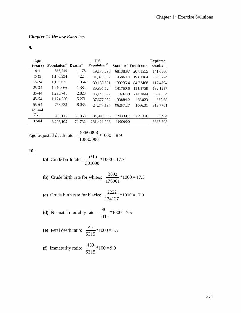
Chapter 14 Exercise Solutions
271
Chapter 14 Review Exercises 9.
Age (years) Populationa Deathsb
U.S. Populationc Standard Death rate
Expected deaths
0-4 566,740 1,178 19,175,798 68138.97 207.8555 141.63065-19 1,140,934 224 41,077,577 145964.4 19.63304 28.65724
15-24 1,130,671 954 39,183,891 139235.4 84.37468 117.479425-34 1,210,066 1,384 39,891,724 141750.6 114.3739 162.125735-44 1,293,741 2,823 45,148,527 160430 218.2044 350.065445-54 1,124,305 5,271 37,677,952 133884.2 468.823 627.6855-64 753,533 8,035 24,274,684 86257.27 1066.31 919.770165 and Over 986,115 51,863 34,991,753 124339.1 5259.326 6539.4Total 8,206,105 71,732 281,421,906 1000000 8886.808
Age-adjusted death rate = 8886.808
*1000 8.91,000,000
=
10.
(a) Crude birth rate: 5315
*1000 17.7301098
=
(b) Crude birth rate for whites: 3093
*1000 17.5176961
=
(c) Crude birth rate for blacks: 2222
*1000 17.9124137
=
(d) Neonatal mortality rate: 40
*1000 7.55315
=
(e) Fetal death ratio: 45
*1000 8.55315
=
(f) Immaturity ratio: 480
*100 9.05315
=
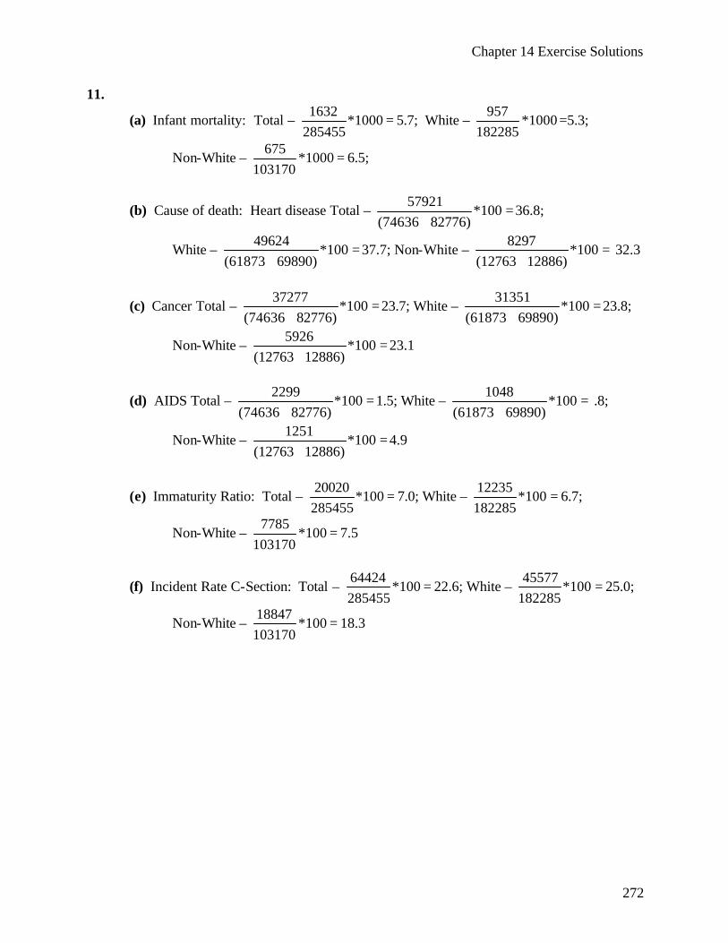
Chapter 14 Exercise Solutions
272
11.
(a) Infant mortality: Total – 1632
*1000285455
= 5.7; White – 957
*1000182285
=5.3;
Non-White – 675
*1000103170
= 6.5;
(b) Cause of death: Heart disease Total – 57921
*100(74636 82776)
=+
36.8;
White – 49624
*100(61873 69890)
=+
37.7; Non-White – 8297
*100(12763 12886)
=+
32.3
(c) Cancer Total – 37277
*100(74636 82776)
=+
23.7; White – 31351
*100(61873 69890)
=+
23.8;
Non-White – 5926
*100(12763 12886)
=+
23.1
(d) AIDS Total – 2299
*100(74636 82776)
=+
1.5; White – 1048
*100(61873 69890)
=+
.8;
Non-White – 1251
*100(12763 12886)
=+
4.9
(e) Immaturity Ratio: Total – 20020
*100285455
= 7.0; White – 12235
*100182285
= 6.7;
Non-White – 7785
*100103170
= 7.5
(f) Incident Rate C-Section: Total – 64424
*100285455
= 22.6; White – 45577
*100182285
= 25.0;
Non-White – 18847
*100103170
= 18.3
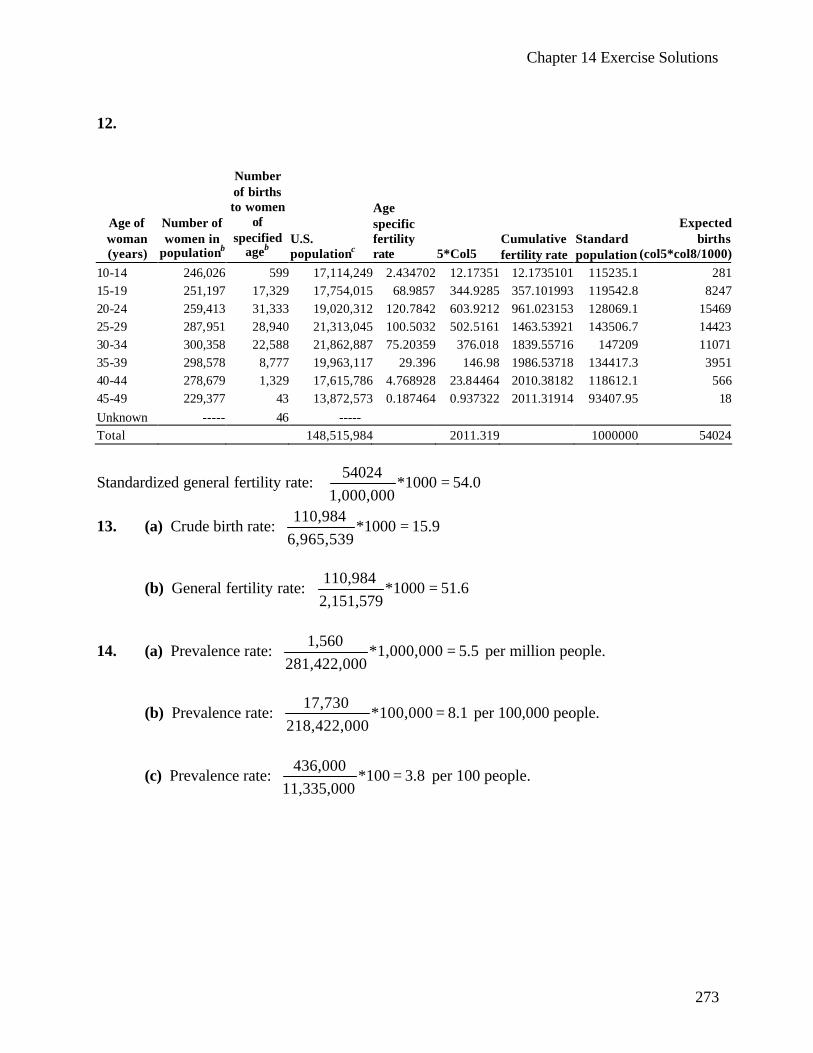
Chapter 14 Exercise Solutions
273
12.
Age of woman (years)
Number of women in
populationb
Number of births to women
of specified
ageb U.S. populationc
Age specific fertility rate 5*Col5
Cumulative fertility rate
Standard population
Expectedbirths
(col5*col8/1000)10-14 246,026 599 17,114,249 2.434702 12.17351 12.1735101 115235.1 281 15-19 251,197 17,329 17,754,015 68.9857 344.9285 357.101993 119542.8 8247 20-24 259,413 31,333 19,020,312 120.7842 603.9212 961.023153 128069.1 15469 25-29 287,951 28,940 21,313,045 100.5032 502.5161 1463.53921 143506.7 14423 30-34 300,358 22,588 21,862,887 75.20359 376.018 1839.55716 147209 11071 35-39 298,578 8,777 19,963,117 29.396 146.98 1986.53718 134417.3 3951 40-44 278,679 1,329 17,615,786 4.768928 23.84464 2010.38182 118612.1 566 45-49 229,377 43 13,872,573 0.187464 0.937322 2011.31914 93407.95 18 Unknown ----- 46 ----- Total 148,515,984 2011.319 1000000 54024
Standardized general fertility rate: 54024
*1000 54.01,000,000
=
13. (a) Crude birth rate: 110,984
*10006,965,539
= 15.9
(b) General fertility rate: 110,984
*1000 51.62,151,579
=
14. (a) Prevalence rate: 1,560
*1,000,000 5.5281,422,000
= per million people.
(b) Prevalence rate: 17,730
*100,000 8.1218,422,000
= per 100,000 people.
(c) Prevalence rate: 436,000
*100 3.811,335,000
= per 100 people.