Unsupervised Bayesian wavelet domain segmentation using a

Potts-Markov random field modeling

Patrice Brault† and Ali Mohammad-Djafari‡

† IEF, Institut d’Electronique Fondamentale, CNRS UMR-8622,

Universite Orsay Paris-Sud, 91405 Orsay Cedex, FRANCE.

‡LSS, Laboratoire des Signaux et Systemes, CNRS UMR-8506,

Supelec, Plateau du Moulon, 91192 Gif sur Yvette Cedex, FRANCE.

patrice.brault@lss.supelec.fr, djafari@lss.supelec.fr

1

Abstract

This paper describes a new fully unsupervised image segmentation method based on a Bayesian approach and a Potts-Markov

Random Field (PMRF) model that are performed in the wavelet domain. ABayesian segmentation model, based on a PMRF

in the direct domain, has already been successfully developed and tested in [23, 12]. This model performs a fully unsupervised

segmentation, on images composed of homogeneous regions, by introducing a hidden Markov Model (HMM) for the regions

to be classified and Gaussian distributions for the noise and for the pixels pertaining to each regions. The computation of

the posterior laws, deduced from these a priori distributions for the pixels, is done by a Markov Chain Monte Carlo (MCMC)

approach and uses a Gibbs sampling algorithm. The use of a high numberof iterations to reach convergence in a segmentation,

where the number of segments, or “classes” labels, is important, makesthe algorithm rather slow for the processing of a large

quantity of data like image sequences [4, 5]. To overcome this problem wehave taken advantage of the property of the wavelet

coefficients, in an orthogonal decomposition, to be modeled by a mixture of two Gaussians. Thus, by projecting an observable

noisy image in the wavelet domain, we are able to segment, in this same domain, the wavelet subbands in only two classes.

After a decomposition up to a scale J, the main idea is to segment the coarse,and small, approximation subband with a high

number of classes, and to segment all the detail (wavelet) subbands withonly two classes. The segmented wavelet domain

coefficients are then reconstructed to obtain a final segmented image in thedirect domain. Our tests on synthetic and natural

images show that the segmentation quality stays good, even with noisy images, and shows that the segmentation times can be

significantly reduced.

Keywords.

Unsupervised segmentation, noisy images, wavelet coefficients domain, Orthogonal Wavelet Decomposition (OWT), unsuper-

vised Bayesian classification, Potts-Markov Random Field (PMRF), Markov Chain Monte Carlo (MCMC) Gibbs sampling.

1 Introduction

Numerous methods for the segmentation of images have been developed and are today available. Statistical methods to which

are closed to our approach can be classified into two main groups :

- Contour based methods. The extraction of contours in an image provides a first way to implement the segmentation of an

image into regions. Markovian modeling as well asMaximum a Posteriori(MAP) deterministic optimization algorithms, like

the Graduated Non-Convexity (GNC) [21] and the Mean Field Annealing (MFA) [27], are used in contour-based methods.

- Region based methods :

Thefirst typeis based on themono-dimensionalmodeling of the histogram, with inter-modes thresholding and Multi-Gaussian

modeling. Also when the image is considered like a realization of a discrete random process, local or global, stochasticat-

tributes can be used. A second type is represented byclusteringmethods [1], hierarchical or not, like K-means, Fuzzy C-means

or Cluster, which is also called ”unsupervised learning” [17], pages xiii and 134, and works by organizing data following an

underlying structure that groups individuals or makes a hierarchy of groups. A third type is finally the one to which our

method pertains and englobes the Markovian methods, supervised and unsupervised. In this last category, we must cite one

2

of the most important works using the regularization and pseudo Maximum Likelihood (pML) in a supervised segmentation

of textured images [13, 14]. More recently, numerous works have been made in the development on wavelet features based

models in a Bayesian segmentation approach.

Our work pertains to the group of region-based segmentationmethods and in particular of unsupervised segmentation meth-

ods. A brief presentation of unsupervised segmentation methods could start with multivariate Gaussian Markov Random Field

(GMRF), models that have been extensively applied for the segmentation of still images [15].

Since several years, the multiscale Bayesian approaches have demonstrated good results in the domain of still image seg-

mentation as well as recently in the domain of animated sequences segmentation. The supervised, partially-unsupervised and

fully unsupervised segmentation of still images with multiscale Bayesian approaches has been widely studied and described

in the literature. Under the Bayesian framework, multiscale approaches have proven to efficiently integrate image features

(like wavelet coefficients) as well as contextual information (like labels in a HMM approach) for the classification. Image

features can be represented by different statistical imagemodels. Contextual information can be obtained by using multiscale

contextual models like, for example, the interscale dependency of class labels between scales in a multiscale approach[2].

Also, the Joint-Multicontext and Multiscale Segmentation(JMCMS) was developed by using the fusion between intra-scale

and inter-scale information [10]. In order to fusing the multiscale contextual information, several methods have beenused : a

Multiscale Random Field (MRF), combined with asequential maximum a posteriori estimator(SMAP), was developed [2, 6].

More recently, the transfer of the observed model to a dual domain like the wavelet domain has enabled to fully take advan-

tage of the very interesting property of wavelet coefficients to be modeled : intra scale, by an Independent Gaussians Mixture

(IGM) and inter scales by considering the evolution of each wavelet coefficient. Models using the evolution of information

between scales, like the wavelet domain Hidden Markov Tree (HMT) [9, 20], and an improved version using the dependencies

across subbands (HTM-3S) [11], have been developed. Also in[7] a multiscale segmentation was developed based on the

HMT and the inter-scale fusion of contextual information. Amethod has also been proposed recently to realize the unsuper-

vised segmentation using HMM in the wavelet domain togetherwith clustering methods [25, 24].

In our group, we have developed a fully unsupervised segmentation also based on a Bayesian approach in the direct domain

[23, 12]. This method uses a HMM for the classification label assigned to the different regions of an image. The difference

of this HMM compared with HMT models is that it is based on a Potts-Markov Random Field (PMRF) for the pixels. This

enables to render the strength of dependency of neighbor pixels to insure a good homogeneity of the region being segmented.

In this direct domain approach the PMRF uses a first order neighborhood. More recently, we have used the same model to

segment2D + T videos sequences, i.e. regularly sampled sequences of images [4]. We have thus demonstrated a significant

improvement in the segmentation of a sequence of images. Turning this result to motion detection and quantification and also

to sequence compression, is being under way and might turn tobe an efficient method amongst other recent developments for

3

motion acquisition, quantification and compression.

Nevertheless, though very efficient for long term segmentation processes, we are also very much interested in reducing the seg-

mentation time. This has motivated a new approach based on the transfer of the segmentation process in the wavelet transform

domain to perform the segmentation. Due to their specific property of fast “local-decay”, the wavelet coefficients, obtained

by decomposition on an orthogonal basis, behave like a mixture of zero-centered Gaussians [18, 9, 20]: a first, high variance,

distribution representative of a few strong coefficients ofmajor importance, and a second, “peaky” low variance distribution

representative of a large number of low magnitude and low importance coefficients. Thus the segmentation of these band-pass

“subband” coefficients can be made using only 2 classes labels. Furthermore, by zeroing coefficients pertaining to the class

of low importance coefficients, we denoise the data and increase the performances of the segmentation, see recent works on

wavelet denoising using Scale Mixture of Gaussians (SMG) in[19]. Based now on a decomposition in the wavelet domain we

found also pertinent to improve the PMRF model used in the direct domain. This is why we adopted a first + second order,

8-connexity model, for the PMRF. This was motivated by the fact that wavelet subbands are split in vertical, diagonal and

horizontal details. We thus tuned the Markov Field neighborhood to the wavelet subbands orientations through a specificα

dependency parameter for the Potts model [26]. So we have naturally fixed three independent parameters:αV , αD andαH as

dependency parameters for our new three-orientations Potts model.

The rest of the paper is organized as follows: Section 2 describes our PMRF-Bayesian unsupervised segmentation method in

the direct domain. Section 3 points out the important properties of the wavelet coefficients and what motivated the choice of

this transform domain to perform the equivalent “dual” of our direct domain segmentation algorithm. Section 4 introduces

our new8-connexity PMRF for the Bayesian segmentation. Section 5 describes in detail the segmentation algorithm in the

wavelet domain, its initialization with the segmentation of its approximation subband, the segmentation of its multiscale detail

subbands in a coarse to fine scale scheme and the final inverse wavelet transform to get the final segmentation in the direct

domain. Sections 6 and 7 make a comparison of the results of our new wavelet-domain Bayesian segmentation with the

same method in the direct domain and with other techniques and recall the important features and advantages of this new

unsupervised Bayesian segmentation in the wavelet domain.

2 Unsupervised segmentation in the direct domain

2.1 Potts-Markov field modeling and Bayesian approach

The description of still image segmentation and fusion by a Bayesian approach and a Hidden Markov Model (HMM) has been

developed and well described by Feron et al. in [12]. We summarize in this section the main steps for the computation of the

posterior laws necessary in the final segmentation-fusion algorithm.

We formulate the segmentation problem as an inverse problemwhere the objective is to find a classificationz(r) of an original

4

imagef(r). The observed imageg(r) is assumed to be a noisy version of the original imagef(r) :

g(r) = f(r) + ǫ(r), r ∈ R (1)

whereR is the set of sitesr of the image.

If we assume the noiseǫ(r) to be centered, white and Gaussian. We have :

ǫ(r) ∝ N (ǫ(r)|0, vǫ) =⇒ p(g(r)|f(r)) = N (g(r)|f(r), vǫ) ∀r ∈ R

If we note by the vectorsg = {g(r), r ∈ R}, f = {f(r), r ∈ R} andǫ = {ǫ(r), r ∈ R} the discretized version of the

images, we can write :

p(g|f) = N (g|f , vǫI) (2)

whereI represents the identity matrix.

Because the goal is to have a reconstructed imagef segmented in a limited number of statistically homogeneousregions, a

hidden variablez, which can take the discrete “label” valuesk ∈ {1, ...,K}, is introduced to represent the imagef classified

in K classes. Such a classification enables to segmentf in regionsRk = {r : z(r) = k}. When regions pertain to the same

class but are not contiguous, the number of segments increases, thus the number of segments is at least equal to the number

of classes. At this point we also make the hypothesis that each region of the segmented image is modeled by a Gaussian

distribution of meanmk and variancevk :

p(f(r)|z(r) = k) = N (f(r)|mk, vk) (3)

So we finally write a model for the distribution of the pixels of the imagef(r) as :

p(f(r)) =

K∑

k=1

αkN (f(r)|mk, vk), with αk = p(z(r) = k) (4)

We can also write the dual expression for the observableg(r) :

p(g(r)|z(r) = k) = N (g(r)|mk, vk + vǫ) (5)

and

p(g(r)) =

K∑

k=1

αkN (g(r)|mk, vk + vǫ), with αk = p(z(r) = k) (6)

In order to build homogeneous regions, the spatial dependency between the label of each pixel (the hidden Markov variable

z(r)) and the label of its neighbors is modeled by a Potts-Markov Random Field (PMRF). The Markovian modeling assumes

5

that the value ofz(r) at a pixel position is related to the value of its neighbors (the four closest vertical and horizontal neighbors

in a first order neighboring). The Potts model enables to control, by means of an attractive/repulsiveα parameter, the mean

value of the size of a region. Thus the homogeneity for each class is proportional to the strength ofα.

p(z(r), r ∈ R) =1

T (α)exp

{

α∑

r∈R

∑

s∈V (r)

δ(z(r) − z(s))

}

(7)

whereV (r) represents the neighborhood ofr. In the sequel of this section we considerV (r) as the first order neighborhood

(4-connexity) of the pixelr.

More explicitly, if we consider a first order neighborhood, this one includes the four pixels of the horizontal and vertical

neighborhoods. The Potts model can be written explicitly with the indices(i, j) of each pixelr(i, j) :

p(z(i, j), (i, j) ∈ R) =1

T (α)× exp

{

αV

∑

(i,j)∈R

δ(z(i, j) − z(i− 1, j))

+ αH

∑

(i,j)∈R

δ(z(i, j) − z(i, j − 1))

}

(8)

where we assumeαV = αH = α.

Using the Bayes rule, the joint posterior law off andz can then be expressed :

p(f ,z|g) ∝ p(g|f ,z) p(f |z) p(z) (9)

The prior laws, defined formerly, need some of their parameters, which are called the modelhyperparameters, to be defined.

These arevǫ, vk andmk. If we want to realize an unsupervised segmentation, the setθ of so-called “hyperparameters” :

θ =

{

vǫ, (mk, vk), k ∈ {1...K}}

(10)

has also to be estimated. For this purpose we also assignprior laws toθ. These prior laws are taken asconjugate priorsand

depend themselves onhyper-hyperparameterswhich areα0, β0,m0 andv0. We refer to [23] for the choice and the values of

these final hyper-hyperparameters. Thepriors for the setθ then takes the form :

p(vǫ) ∼ IG(vǫ|αǫ0, β

ǫ0)

p(mk) ∼ N (mk|mk0 , v

k0 ) , k = {1...K}

p(vk) ∼ IG(vk|αk0 , β

k0 ) , k = {1...K}

(11)

whereIG is the Inverse-Gamma.

6

The expression of the posterior law for an unsupervised segmentation becomes finally :

p(f ,z,θ|g) ∝ p(g|f ,z,θ) p(f |z,θ) p(z) p(θ) (12)

2.2 Markov-Chain Monte-Carlo (MCMC) and Gibbs sampling algorit hm

The Bayesian approach consists now in estimating the whole set of variables(f ,z,θ) following the jointa posterioridistribu-

tion p(f ,z,θ|g) after Eq. 12. The MCMC method consists in generating samplesfrom thisposteriorlaw from which we can

estimate the mean, the median or any other statistics for each variablef , z or θ. For example the mean value off becomes :

f =

∫

f . p(f |g)df ≃ 1

N

N∑

n=1

f (n) (13)

wheref (n) are samples drawn fromp(f |g).

To generate samples from the joint distribution in Eq. 12, weuse the following Gibbs sampling algorithm :

fn ∼ p(f |g,z(n−1),θ(n−1))

zn ∼ p(z|g,θ(n−1),f (n−1)

θn ∼ p(θ|g,z(n−1),f(n−1)

)

(14)

where we need to write the expressions of those three posterior laws :

1) for f

p(f |g,z,θ) ∝ p(g|f ,z,θ) p(f |z,θ)

∝ ∏

k

∏

r∈Rk

N (g(r)|f(r), vǫ)N (f(r)|mk, vk)

∝ ∏

k

∏

r∈Rk

N (f(r)|mk, vk)

(15)

with mk = vk

(

mk

vk

+

Pr∈Rk

g(r)

vǫ

)

, vk =(

1vǫ

+ 1vk

)−1

and Rk = {r : z(r) = k}

2) for z

p(z|g,f ,θ) ∝ p(g|f ,z,θ) p(f |z,θ) p(z|θ)

∝[

∏

k

p(gk|fk, vǫ) p(fk|mk, vk)

]

p(z)

∝[

∏

k

∏

r∈Rk

N (f(r)|mk, vk)

]

p(z)

(16)

We can notice that this posterior law is also a PMRF where the prior probabilities are weighted by the posterior likelihood.

3) for θ

7

p(θ|f , g,z) ∝ p(vǫ|f , g)∏

k

p(mk|vk,f ,z).p(vk|f ,z) (17)

where :

- For the noise : p(vǫ|f , g) ∝ IG(vǫ, |α, β), with α = n/2 + αǫ0 andβ = 1

2

∑

r∈R

(g(r) − f(r))2 + βǫ0

andn = Card(R), is the total number of pixels.

- For the mean in each regionk : p(mk|f ,z, vk,m0, v0) ∝ N (mk|µk, ξk)

with µk = ξk

(

mk

0

vk

0

+

Pr∈Rk

f(r)

vk

)

, ξk =(

nk

vk

+ 1vk

0

)−1

, and nk = Card(Rk)

- For the variance in each regionk : p(vk) ∝ IG(vk|αk, βk)

with αk = αk0 + nk

2 , and βk0 = β0 + 1

2

∑

r∈Rk

(f(r) −mk)2

This algorithm is iterated a “sufficient” number of times (itermax) in order to reach the convergence of the segmentation.

We do not use any real “convergence criterion” and by convergence we mean that the segmented regions do not change

significantly in the next iterations. After convergence, wetake the max(histogram) for each pixel value and for all iterations.

Also, our experience on the images analyzed has showed us that itermax depends essentially on the complexity of the image

and the number of luminance levels, as well as on the number ofclasses taken for the segmentation. In general for a number

of classesK = 4 we takeitermax between20 and50. If we generate a number of samplesitermax = N ,

(f ,z,θ)(1), (f ,z,θ)(2), ...(f ,z,θ)(L), ..., (f ,z,θ)(N)

the algorithm starts providing homogeneous segments only after a “heating time” of L samples. The final value for each pixel

is given by the median, the maximum of its histogram or the mean of the(N − L) last values :

(f , z, θ) ≃ 1

(N − L)

N∑

n=L+1

(f ,z,θ)n (18)

3 Projection in the wavelet domain

As mentioned in the introduction, our Bayesian segmentation method, based on a Potts-Markov random field modeling in

the direct domain, gives good classification results. Nevertheless the main drawback of such an algorithm, using iterative

sampling, is to exhibit very important computation times. For one of our concerns is to perform the segmentation on video

sequences, we are interested in lowering these computationtimes. Using the projection of the observable onto a transform

domain can provide interesting properties. In particular the wavelet domain coefficients exhibit properties that are very inter-

8

esting for our segmentation application :

- It gives a sparse representation of the observable.

- It presents the property of fast local decay of the wavelet coefficients that enables a modeling of these coefficients by a

mixture of two Gaussians.

- It reflects, by analyzing the evolution of the wavelet coefficients between scales, the strength of singularities (Holder coeffi-

cients) of each pixel of an image, and in the same way can modelthe dependency of pixels between scales.

More precisely it has been established [8, 9, 20] that the wavelet coefficients of “real-world” signals exhibit a local decay

property which means that the coefficients of highest energy, and of utmost representativity for the signal, are very sparse and

that the coefficients of low energy, and of low importance forthe signal, are in large quantity. In the probability domain, we

can then express the marginal density of the wavelet coefficients by one spread and heavy-tailed, i.e. with a large variance,

Gaussian density, for the important coefficients, and by another very peaky, and low variance, Gaussian density for the coeffi-

cients of low importance. Such a property is well expressed by a mixture of Gaussians and the coefficients can be considered

approximately decorrelated due to the Orthogonal Wavelet Transform (OWT) decomposition used (Fig. 2).

As a result of this we may notice that the model of mixture of two Gaussians can be very interesting when performing our

Bayesian segmentation in the wavelet domain. It means that the segmentation in the wavelet subbands can be done by using

only two classes. Then making a projection of the observableg, segmenting the coarse approximation subband with a high

number of classes and finally segmenting the successive detail subbands with only two classes up to the image resolution

significantly reduces the segmentation cost.

We will now introduce the wavelet decomposition, then will describe the complete segmentation algorithm in the wavelet

domain.

In order to proceed with the same Bayesian segmentation approach in the wavelet domain, we first need to decompose the

observableg on an orthogonal basis of scaling and wavelet functions. We use the classical multiresolution pyramidal decom-

position of Mallat. This decomposition uses shifted and dilated versions of the scalingφ and waveletψ functions.

The observableg is written as a function of its decomposition coefficients,aJ,b1,b2 anddBj,b1,b2

, as :

g(x, y) =∑

(b1,b2)∈Z

aJ,b1,b2φLLJ,b1,b2

(x, y) +∑

B∈B

∑

j6J

∑

(b1,b2)∈Z

dBj,b1,b2

ψBj,b1,b2

(x, y) (19)

whereφLLj,b1,b2

= 2−jφ(2−jx − b1, 2−jy − b2), ψB

j,b1,b2= 2−jψB(2−jx − b1, 2

−jy − b2) andB = {HL,LH,HH}. The

HL, LH and HH are called the details, or wavelet, subbands. L and H represent the low and high pass band conjugate mirror

filters, respectivelyh andg. Thus HL correspond to the vertical, LH to the horizontal andHH to the diagonal subband. LL is

called the approximation, or scaling, subband.

9

The decomposition coefficients are expressed as :

aJ,b1,b2 =

∫

R2

g(x, y)φLLJ,b1,b2

dxdy (20)

and

dBj,b1,b2

=

∫

R2

g(x, y)ψBj,b1,b2

dxdy (21)

In the sequel we will use the notationVJ , WVj , WD

j andWHj , respectively for the subbands LL,HL,LL and LH.WV

j , WDj

andWHj are respectively the vertical, diagonal and horizontal detail subbands. The corresponding wavelet filters are given

by :

WVj → ψjφj [~b]

WDj → ψjψj [~b]

WHj → φjψj [~b]

(22)

The decomposition of our observableg is done from the initial resolutionL = 0 or 2L up to the scaleJ or 2J . Decomposing

on two scale means thatJ = 2 and the scaling parameter isj ∈ 0, 1, ..., J . The corresponding resolution to a scale is obtained

by the inverse power2−j . The confusion between scale and resolution is easy and in the sequel we will try to stay as clear as

possible in the description of the algorithm starting from the coarsest scale (the highestj).

With this notation, the decomposition of our observableg in the wavelet domain can also be expressed as :

g(g, Vj ,Wj) = P (g, VJ) +

J∑

j=1

P (g,Wj) (23)

The figures below describe the application of the wavelet orthogonal transform on one band of an hyperspectral (224 spectral

bands) image of a satellite view. The figures 2 b) and c) show respectively the histograms of the approximation coarse

subband and of the detail diagonal coarse subband. As previously said, the first histogram can be modeled by a mixture of

several independent Gaussians, which motivates the segmentation of this approximation subband in a high number of labels.

Conversely the second histogram of the detail diagonal subband can be modeled by a mixture of two independent Gaussians

(which is more visible in the lin-log representation), one with a high variance (sparse high value coefficients) and one with a

low variance (numerous low value coefficients) and the segmentation in all detail subbands is thus done with only two labels.

10

Figure 1:a) Original image of the Channel 100 of an hyperspectral satellite image composed of 224 channels. b) Pyramidal representation

of the Fast Orthogonal Wavelet 2-levels decomposition applied to the the channel 100 of our hyperspectral image. Here the lettern can be

replaced byJ , the scale parameter at the coarsest scale2J bands.

200 300 400 500 600 700 800 900 10000

20

40

60

80

100

120

140An0

−200 −150 −100 −50 0 50 100 150 2000

100

200

300

400

500

600Dn0d

Figure 2: a) Histogram of theAJ (or An), the approximation coefficients at the coarsest scale. b) Histogram ofAJ described by a mixture

of multiple Gaussians, one for each class. c) Histogram of theDD

J (or DD

n ), the detail diagonal coefficients at the coarsest scale. d) Linlog

histogram of theDD

J explaining the choice of a two independent Gaussians mixture model, with one large and one small variance.

4 Eight connexity, first and second order Potts-Markov random field

4.1 Model description

In order to find statistically homogeneous regions for the segments, our Markovian segmentation method in the direct domain

uses a Potts-Markov random field [12] to define the spatial dependency of the labels in the HMM. In this direct model, the

dependency of the pixel label is searched in a first order neighborhood. Nevertheless and due to the fact that the segmentation

is done now in the wavelet domain, we have to take into accountthat this spatial dependency is quite different than in the direct

domain due to the fact that the three “detail” subbands are oriented in the vertical, diagonal (D1 = π/4 andD2 = 3π/4 ) and

horizontal directions. This prior knowledge is taken into account by introducing these orientations in a new “eight-connexity”

(or neighborhood of orders 1 and 2) Potts-Markov Random Field. The new model of the PMRF can be written:

11

p(z(i, j), (i, j) ∈ R) = 1T (αV ,αD1

,αD2,αH) × exp

{

+αV

∑

(i,j)∈R

δ(z(i, j) − z(i− 1, j))

+αD1

∑

(i,j)∈R

δ(z(i, j) − z(i+ 1, j − 1))

+αD2

∑

(i,j)∈R

δ(z(i, j) − z(i− 1, j − 1))

+αH

∑

(i,j)∈R

δ(z(i, j) − z(i, j − 1))

}

(24)

The parametersαV , αD1, αD2andαH respectively control the degree of spatial dependency of the z variable in the directions

V ,D1,D2 andH. For the wavelet “diagonal” subband we gather theD1 andD2 dependencies in one diagonalD1D2 depen-

dency. For the first, coarse, approximation subband, we alsogather theV andH dependency in aV H dependency which is

equivalent to the first-order dependency (first order neighborhood) used in the direct-domain implementation.

Also, in order to accelerate the sampling of the image sites,we implement the MCMC-Gibbs algorithm “in parallel” [12]. If

we consider, for theV H dependency, that the label value of one site is conditional to the label values of the sites of its first

order neighboring (p(z(i, j)|z(i, j − 1), z(i− 1, j)), then all the pixel sites corresponding to the white (odd numbered) cases

of a chessboard can be considered as independent (Fig. 4 a)).In a same way all the black cases (even numbered) of this chess-

board can be considered as independent conditionally to thevalues of the white sites in their first order neighborhood. Thus

we are able, once all the white cases are sampled, to sample all the black cases in only one iteration due to the independency

of the sites. With this scheme, the whole image can be sampledin two successive iterations, one on the black sites and one on

the white sites.

Similarly, for theD1D2 dependencies, we can also use an implementation “in parallel” of the Gibbs sampler, but by using a

different scheme for the independent sites. The image is then split in two sets of interlaced black and white sites which enables

to consider each type of sites as independent conditionallyto the knowledge of the sites of the second order neighboring.

The application of our new PMRF model to the wavelet subbandsis done by deleting the PMRF terms that do not apply to

the subband concerned. Moreover theαV parameter used in this “vertical” term can be adjusted to anypositive value, which

means that we assign a specified, non null, dependency strength between the labels z of the region concerned. As we have seen

in [12], this means that the higher theα parameter, the higher thea priori of a little number of great homogeneous regions. For

the first, coarse, approximation subband, we also gather theV andH dependency in aV H dependency which is equivalent

to the first-order dependency used in the direct-domain implementation.

12

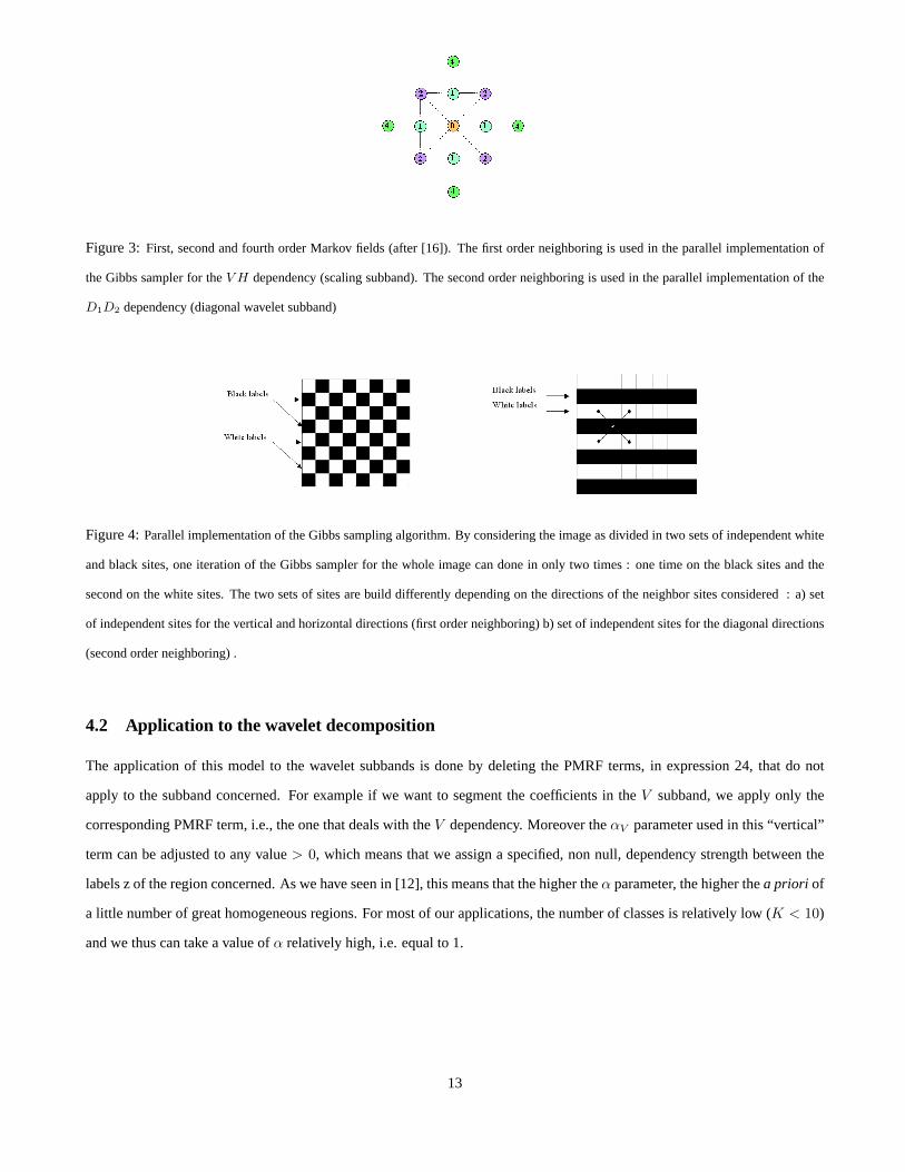
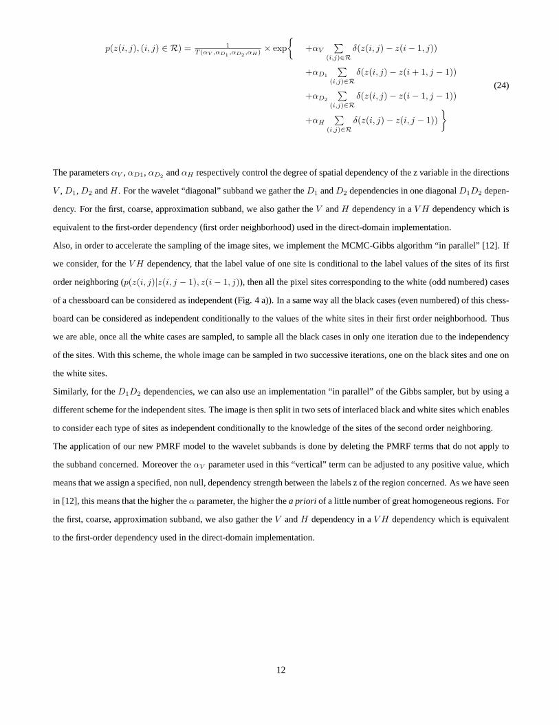
Figure 3:First, second and fourth order Markov fields (after [16]). The firstorder neighboring is used in the parallel implementation of

the Gibbs sampler for theV H dependency (scaling subband). The second order neighboring is used in the parallel implementation of the

D1D2 dependency (diagonal wavelet subband)

Figure 4:Parallel implementation of the Gibbs sampling algorithm. By considering the image as divided in two sets of independent white

and black sites, one iteration of the Gibbs sampler for the whole image can done in only two times : one time on the black sites and the

second on the white sites. The two sets of sites are build differently depending on the directions of the neighbor sites considered : a) set

of independent sites for the vertical and horizontal directions (first order neighboring) b) set of independent sites for the diagonal directions

(second order neighboring) .

4.2 Application to the wavelet decomposition

The application of this model to the wavelet subbands is doneby deleting the PMRF terms, in expression 24, that do not

apply to the subband concerned. For example if we want to segment the coefficients in theV subband, we apply only the

corresponding PMRF term, i.e., the one that deals with theV dependency. Moreover theαV parameter used in this “vertical”

term can be adjusted to any value> 0, which means that we assign a specified, non null, dependencystrength between the

labels z of the region concerned. As we have seen in [12], thismeans that the higher theα parameter, the higher thea priori of

a little number of great homogeneous regions. For most of ourapplications, the number of classes is relatively low (K < 10)

and we thus can take a value ofα relatively high, i.e. equal to 1.

13

5 Bayesian segmentation in the wavelet domain

The initial operation to perform on the image to be segmented, is first to do its decomposition on an orthogonal wavelet basis.

The decomposition used here is the classical Mallat pyramidal transform of complexityO(N2). This transform enables to

get wavelet coefficients which are split in two main classes :the weak and the strong coefficients. Noticing this point on the

wavelet coefficients has an important incidence for segmentation purposes : it enables to segment the “detail” images with

only two classes (K = 2). On complex images, i.e. the first “approximation” subband, the segmentation will be led with a

higher number of classes, e.g.K = 8.

Algorithm description

Our segmentation scheme in the wavelet domain is based on a coarse to fine scale scheme (Fig. 5). The Bayesian segmenta-

tion is performed on the wavelet subband coefficients and at all scales with a low valueK = 2, except for the approximation

coefficients. The segmentation starts from theg observation projected into the wavelet domain. The segmentation algorithm

can be described with the following steps:

1) Wavelet decomposition to the orderJ , i.e. down to scale2J , on an orthogonal basis (Haar wavelet). This wavelet is chosen

for its property w.r.t. image discontinuities, a property that we are going to use within the next steps.

2) We segment the approximation coefficientsVJ at scale2J with the number of classes desired in the final segmentation,e.g.

K = 8. For the Gibbs sampling, and with a large value ofK, the iteration number is given a high value in order to assurethe

convergence.

3) In the segmented image of the approximationsz(VJ), we detect (by derivation) the regions exhibiting vertical, diagonal

(π/4 and3π/4) and horizontal discontinuities.

4) At this same scale, the3 detail subbandsWVJ ,WD

J andWHJ are segmented and we respectively use, as an initializationof

these segmentations, the 3 subsets of discontinuitiesdiffV , diffD anddiffH computed at the former step. This step is realized

with a weak number of classes (K = 2) and of iterations of the Gibbs sampling.

5) The 3 segmented detail subbands are upsampled by 2 in orderto repeat the process at the next upper level.

6) We segment the 3 detail subbandsWV(J−1), W

D(J−1) andWH

(J−1) on the basis of the initialization obtained in the former

step. The same process is then repeated up to the image resolution level.

7) We reconstruct the segmented image starting from the coarsest scale2J of the decomposition. The reconstruction uses:

- for the initial approximation scale (level2J ): the average of the original scaling coefficients within each region of the seg-

mented approximation subband:(VJ(zk)) with k ∈ 1, ...,K.

- for all the detail subbands: the original wavelet coefficients,W (V,D,H)j∈{1...J}, for the segments that pertain to the classk = 2. The

coefficients pertaining to the classk = 1 are cancelled.

14

8) We re-classify the histogram, in the direct domain, of thesegmented image obtained in the former step. This is done by

finding the thresholdsThjM , j ∈ {1...(K + 1)} of the modes of this histogram. This re-classification is necessary because

there is no reason for the wavelet coefficients to pertain, after inversion, to a perfect classification inK classes. This step is

easily realized by using theK meansmk computed at the coarsest approximation scaleVJ and used now to find the histogram

modes thresholds by simply taking the mid-point of the meansfor each couple of successive classes :ThjM = mk+1+mk

2 . We

also take, as value for the first and the last thresholds,Th1M andThK+1

M , respectively the minimum and maximum values of

the pixels.

9) The re-classification of the histogram is done in the same loop as the new labeling of the pixels inK successive classes,

which provides at the same time the final segmented image inK classes withK starting from1.

From a first point of view, this approach, based on the initialization of the segmentation of the coarse detail subbands from

the discontinuities in the segmentation of the approximation subband, can be considered as a way to take into account the

intra-scaledependency of the wavelet coefficients. From a second point of view, the initialization of the segmentation of

detail subbands at a scalej, by the segmentation of the detail subbands at the immediatecoarser scalej + 1, can also be

considered as a way to take into account theinter-scaledependency of the wavelet coefficients.

Remark : the only parameters to choose before starting the computation are the maximum number of iterations,itermax,

of the Gibbs sampling algorithm, and the numberK of classes requested.itermax is generally taken large enough to assure

the convergence of the segmentation, i.e. between20 and50. K must be taken at least equal to the number of classes in the

image, if this value is known. The value ofK will automatically decrease to fit the maximum number of classes in the image,

but will not increase. Nevertheless, if the number of iterations is too low, the algorithm will not converge towards the correct

number of classes and will give a value between the value asked and the real value (see Fig. 8). If the number of classes is

unknown, thenK must be chosen accordingly to the purpose of the application.

In a natural image, this number is generally taken between two and ten. Among other adjustable parameters are theαpotts

parameter, i.e.αV , αVW , αD

W andαHW for the approximation and detail subbands.αV , α

VW , αD

W andαHW are generally fixed to

1. Nevertheless, this parameter can be adjusted, especiallyfor some natural images. The possibility to adjust separately αV in

the coarse approximation subband andαVW , αD

W andαHW in the detail subbands enables to get smaller or larger homogeneous

regions in the initial segmentation of the coarse approximation subband and to give more or less importance to the disconti-

nuities in this subband and thus to the size of the regions in the wavelet subbands. These parameters, tested on some natural

images, can be efficiently trimmed between0.5 and5. Another important initial parameter is thez0 initial segmentation of

the observable, if we own a liable knowledge of it. It is this same initialization parameter that we use, between subbands,

in our algorithm, to improve the segmentation speed. The parametersmk, vk andvǫ can also be initially fixed if we have a

15

knowledge of them. In any other cases all these parameters can be left to their default initial values and will be automatically

computed.

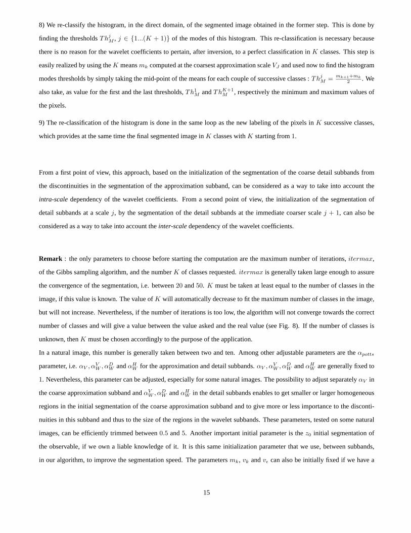
Figure 5:Wavelet domain Bayesian segmentation scheme. The observed datag is first decomposed in the wavelet domain (2 scales shown

here). It is then segmented in this domain, with six labels for the approximation subband and two labels for all the detail subbands. The

approximation subband is filtered by replacing the valuez(r) = k of each classk by the average of the initial scaling coefficients. All the

wavelet subbands are filtered by zeroing the coefficients pertaining to theclassk = 1 of “weak coefficients” and by leaving the coefficients

of classk = 2 at their initial value. The final segmentation is obtained by reconstruction in the direct domain and histogram reclassification.

16

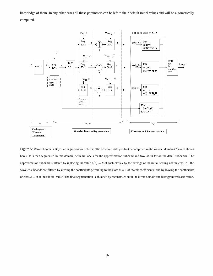
Figure 6:a) Mallat’s pyramidal representation of the segmented imagez. The approximation part is segmented in6 classes (color part).

The detail subbands are represented in black for the class of the weak coefficients, that are zeroed, and in white for the class of the strong

coefficients that will be used for the final reconstruction. b) Reconstruction result of the wavelet segmentation shown in the direct domain.

6 Results and comparison

In this section we show comparative results on three examples of test images. The first test image is a synthetic mosaic image,

“texmos3.s1024” that we upsampled from the texmos3.s512 image of the SIPI [22] database and that we have perturbed with

additive Gaussian noises of different variances for the regions and for the whole image. The second test image is a natural

image of the SIPI database representing the San Diego coast at Point Loma. The third image comes from one band of an

hyperspectral AVIRIS satellite image of the earth and takenamongst the224 contiguous channels of this ”3D” image.

Four segmentation algorithms are compared : (1) the direct domain Bayesian Potts-Markov Segmentation (BPMS), (2) the

Wavelet Bayesian Potts-Markov Segmentation (WBPMS) presented in this paper, (3) the HMT segmentation from [7] and (4)

two versions of a clustering K-means algorithm with two different distance measures.

For the first example we have tested the algorithms 1, 2 and 4. For the second example we have tested the algorithms 1, 2 and

3. For the last example (our hyperspectral image), we have compared the methods 1 and 2.

To evaluate the segmentation quality, we use the numerical ”Pa” criterion which is thepercentageof pixels that are correctly

classified, showing theaccuracyof the segmentation [25, 24]. This test is used of course for synthetic images (our first test)

with a knownz classification.

We also indicate for each of the tests the computation time which is an important challenge for us. All computations have been

done on a 1.6Mhz Pentium M, with 1MB of cache-RAM and 512MB System-RAM, which is not an optimal configuration

for running image processing algorithms. This let us suppose that on a dedicated image processing machine, and a parallel

architecture, we would reach much lower computation times.

17

6.1 First example

In this example we use the ”texmos3.s1024” mosaic of the SIPI(Signal and Image Processing Institute) database of the USC

(University of Southern California). This mosaic is a512 × 512, 8 bits, image, upsampled to1024 × 1024 composed of

23 regions and 8 classes of homogeneous (not textured) regions. We have upsampled this image in order to demonstrate the

WBPMS on four scales of decomposition, which enables to startsegmenting a not too small approximation subband of size

64 × 64 pixels. In order to model a more complex image, we have super-imposed additive Gaussian noises with different

variances for each class to this texmos3s mosaic. Furthermore, a global Gaussian noise with another variance has been added

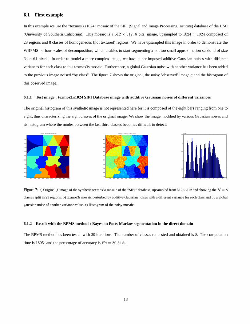
to the previous image noised “by class”. The figure 7 shows theoriginal, the noisy ’observed’ imageg and the histogram of

this observed image.

6.1.1 Test image : texmos3.s1024 SIPI Database image with additive Gaussian noises of different variances

The original histogram of this synthetic image is not represented here for it is composed of the eight bars ranging from one to

eight, thus characterizing the eight classes of the original image. We show the image modified by various Gaussian noisesand

its histogram where the modes between the last third classesbecomes difficult to detect.

z image; texmos3−s1024−orig

100 200 300 400 500 600 700 800 900 1000

100

200

300

400

500

600

700

800

900

1000

z image; texmos3−s1024−noisy

100 200 300 400 500 600 700 800 900 1000

100

200

300

400

500

600

700

800

900

1000

0 1 2 3 4 5 6 7 8 9 100

0.5

1

1.5

2

2.5x 10

4

Figure 7:a) Originalf image of the synthetic texmos3s mosaic of the ”SIPI” database, upsampled from512×512 and showing theK = 8

classes split in23 regions. b) texmos3s mosaic perturbed by additive Gaussian noises witha different variance for each class and by a global

gaussian noise of another variance value. c) Histogram of the noisy mosaic.

6.1.2 Result with the BPMS method : Bayesian Potts-Markov segmentation in the direct domain

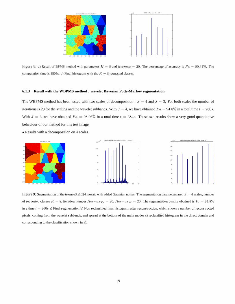
The BPMS method has been tested with20 iterations. The number of classes requested and obtained is8. The computation

time is 1805s and the percentage of accuracy isPa = 80.34%.

18

texmos3−s1024−noisy Seg Bay direct

100 200 300 400 500 600 700 800 900 1000

100

200

300

400

500

600

700

800

900

1000

0 1 2 3 4 5 6 7 80

0.5

1

1.5

2

2.5x 10

5 INPD−DirSeg−hist Bins: 100

Figure 8: a) Result of BPMS method with parametersK = 8 anditermax = 20. The percentage of accuracy isPa = 80.34%. The

computation time is 1805s. b) Final histogram with theK = 8 requested classes.

6.1.3 Result with the WBPMS method : wavelet Bayesian Potts-Markov segmentation

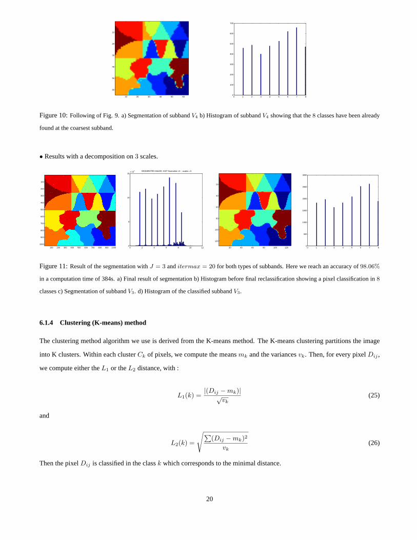
The WBPMS method has been tested with two scales of decomposition : J = 4 andJ = 3. For both scales the number of

iterations is20 for the scaling and the wavelet subbands. WithJ = 4, we have obtainedPa = 94.8% in a total timet = 260s.

With J = 3, we have obtainedPa = 98.06% in a total timet = 384s. These two results show a very good quantitative

behaviour of our method for this test image.

• Results with a decomposition on4 scales.

IWT−SEG−CLASS

100 200 300 400 500 600 700 800 900 1000

100

200

300

400

500

600

700

800

900

1000

0 2 4 6 8 10 12 140

2

4

6

8

10

12x 10

4 SEGMENTED IMAGE; HIST Normalisé >0 ; scales =4

0 1 2 3 4 5 6 7 80

2

4

6

8

10

12

14

16

18x 10

4 Reclassified Wave Segmented Image ; scales =4

Figure 9:Segmentation of the texmos3.s1024 mosaic with added Gaussian noises. The segmentation parameters are :J = 4 scales, number

of requested classesK = 8, iteration numberItermaxVJ= 20, ItermaxW = 20. The segmentation quality obtained isPa = 94.8%

in a timet = 260s a) Final segmentation b) Non reclassified final histogram, after reconstruction, which shows a number of reconstructed

pixels, coming from the wavelet subbands, and spread at the bottom of the main modes c) reclassified histogram in the direct domain and

corresponding to the classification shown in a).

19

10 20 30 40 50 60

10

20

30

40

50

60

0 1 2 3 4 5 6 7 80

100

200

300

400

500

600

700

Figure 10:Following of Fig. 9. a) Segmentation of subbandV4 b) Histogram of subbandV4 showing that the8 classes have been already

found at the coarsest subband.

• Results with a decomposition on3 scales.

100 200 300 400 500 600 700 800 900 1000

100

200

300

400

500

600

700

800

900

1000

0 2 4 6 8 10 120

5

10

15x 10

4 SEGMENTED IMAGE; HIST Normalisé >0 ; scales =3

20 40 60 80 100 120

20

40

60

80

100

120

0 1 2 3 4 5 6 7 80

500

1000

1500

2000

2500

3000

Figure 11:Result of the segmentation withJ = 3 anditermax = 20 for both types of subbands. Here we reach an accuracy of98.06%

in a computation time of 384s. a) Final result of segmentation b) Histogram before final reclassification showing a pixel classification in8

classes c) Segmentation of subbandV3. d) Histogram of the classified subbandV3.

6.1.4 Clustering (K-means) method

The clustering method algorithm we use is derived from the K-means method. The K-means clustering partitions the image

into K clusters. Within each clusterCk of pixels, we compute the meansmk and the variancesvk. Then, for every pixelDij ,

we compute either theL1 or theL2 distance, with :

L1(k) =|(Dij −mk)|√

vk

(25)

and

L2(k) =

√

∑

(Dij −mk)2

vk

(26)

Then the pixelDij is classified in the classk which corresponds to the minimal distance.

20

SEG−BY−CLASS; L1 ;texmos3−s1024−noisy

100 200 300 400 500 600 700 800 900 1000

100

200

300

400

500

600

700

800

900

1000

0 1 2 3 4 5 6 7 80

0.5

1

1.5

2

2.5

3

3.5

4x 10

5

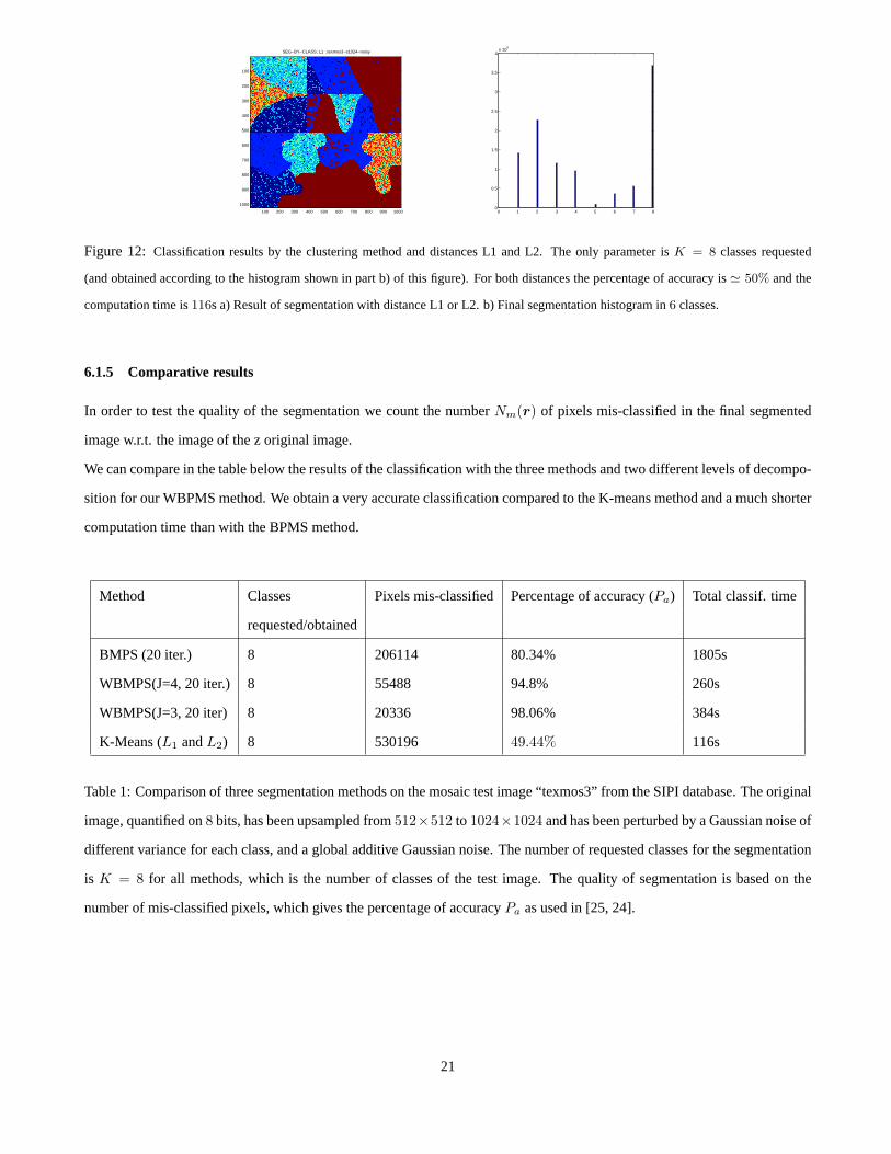
Figure 12: Classification results by the clustering method and distances L1 and L2. Theonly parameter isK = 8 classes requested

(and obtained according to the histogram shown in part b) of this figure).For both distances the percentage of accuracy is≃ 50% and the

computation time is116s a) Result of segmentation with distance L1 or L2. b) Final segmentation histogram in6 classes.

6.1.5 Comparative results

In order to test the quality of the segmentation we count the numberNm(r) of pixels mis-classified in the final segmented

image w.r.t. the image of the z original image.

We can compare in the table below the results of the classification with the three methods and two different levels of decompo-

sition for our WBPMS method. We obtain a very accurate classification compared to the K-means method and a much shorter

computation time than with the BPMS method.

Method Classes Pixels mis-classified Percentage of accuracy (Pa) Total classif. time

requested/obtained

BMPS (20 iter.) 8 206114 80.34% 1805s

WBMPS(J=4, 20 iter.) 8 55488 94.8% 260s

WBMPS(J=3, 20 iter) 8 20336 98.06% 384s

K-Means (L1 andL2) 8 530196 49.44% 116s

Table 1: Comparison of three segmentation methods on the mosaic test image “texmos3” from the SIPI database. The original

image, quantified on8 bits, has been upsampled from512×512 to 1024×1024 and has been perturbed by a Gaussian noise of

different variance for each class, and a global additive Gaussian noise. The number of requested classes for the segmentation

is K = 8 for all methods, which is the number of classes of the test image. The quality of segmentation is based on the

number of mis-classified pixels, which gives the percentageof accuracyPa as used in [25, 24].

21

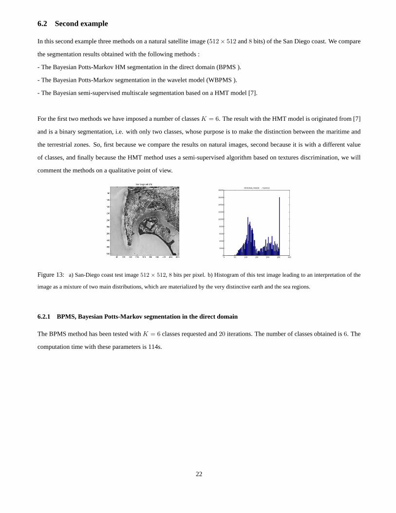
6.2 Second example

In this second example three methods on a natural satellite image (512× 512 and8 bits) of the San Diego coast. We compare

the segmentation results obtained with the following methods :

- The Bayesian Potts-Markov HM segmentation in the direct domain (BPMS ).

- The Bayesian Potts-Markov segmentation in the wavelet model (WBPMS ).

- The Bayesian semi-supervised multiscale segmentation based on a HMT model [7].

For the first two methods we have imposed a number of classesK = 6. The result with the HMT model is originated from [7]

and is a binary segmentation, i.e. with only two classes, whose purpose is to make the distinction between the maritime and

the terrestrial zones. So, first because we compare the results on natural images, second because it is with a different value

of classes, and finally because the HMT method uses a semi-supervised algorithm based on textures discrimination, we will

comment the methods on a qualitative point of view.

0 50 100 150 200 250 3000

2000

4000

6000

8000

10000

12000

14000

16000

18000ORIGINAL IMAGE ; 512x512

Figure 13: a) San-Diego coast test image512 × 512, 8 bits per pixel. b) Histogram of this test image leading to an interpretation of the

image as a mixture of two main distributions, which are materialized by the verydistinctive earth and the sea regions.

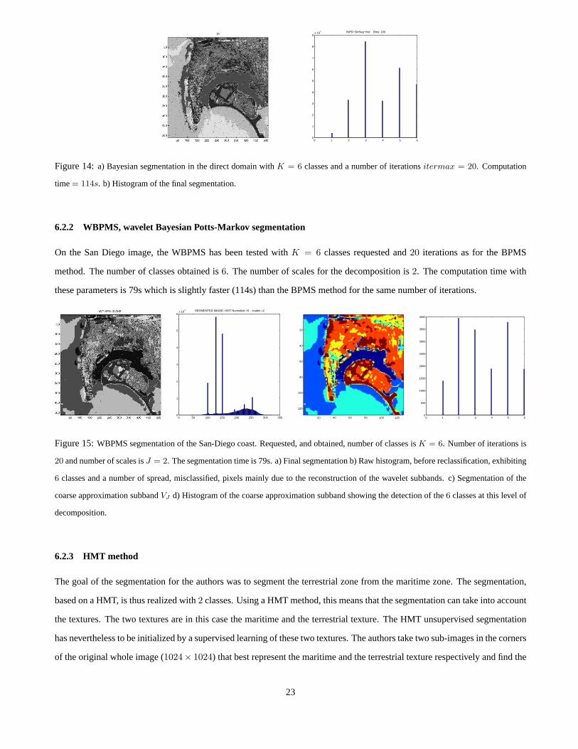
6.2.1 BPMS, Bayesian Potts-Markov segmentation in the directdomain

The BPMS method has been tested withK = 6 classes requested and20 iterations. The number of classes obtained is6. The

computation time with these parameters is 114s.

22

0 1 2 3 4 5 60

1

2

3

4

5

6

7

8

9x 10

4 INPD−DirSeg−hist Bins: 100

Figure 14:a) Bayesian segmentation in the direct domain withK = 6 classes and a number of iterationsitermax = 20. Computation

time= 114s. b) Histogram of the final segmentation.

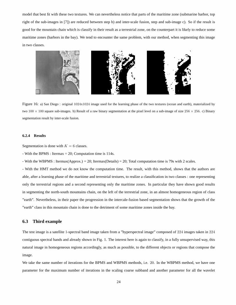
6.2.2 WBPMS, wavelet Bayesian Potts-Markov segmentation

On the San Diego image, the WBPMS has been tested withK = 6 classes requested and20 iterations as for the BPMS

method. The number of classes obtained is6. The number of scales for the decomposition is2. The computation time with

these parameters is 79s which is slightly faster (114s) thanthe BPMS method for the same number of iterations.

0 50 100 150 200 250 300 3500

1

2

3

4

5

6x 10

4 SEGMENTED IMAGE; HIST Normalisé >0 ; scales =2

20 40 60 80 100 120

20

40

60

80

100

120

0 1 2 3 4 5 60

500

1000

1500

2000

2500

3000

3500

4000

Figure 15:WBPMS segmentation of the San-Diego coast. Requested, and obtained, number of classes isK = 6. Number of iterations is

20 and number of scales isJ = 2. The segmentation time is 79s. a) Final segmentation b) Raw histogram, before reclassification, exhibiting

6 classes and a number of spread, misclassified, pixels mainly due to the reconstruction of the wavelet subbands. c) Segmentation of the

coarse approximation subbandVJ d) Histogram of the coarse approximation subband showing the detection of the6 classes at this level of

decomposition.

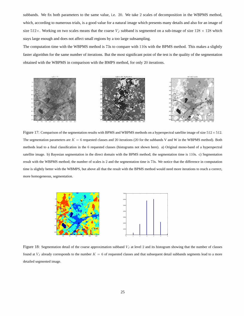
6.2.3 HMT method

The goal of the segmentation for the authors was to segment the terrestrial zone from the maritime zone. The segmentation,

based on a HMT, is thus realized with2 classes. Using a HMT method, this means that the segmentation can take into account

the textures. The two textures are in this case the maritime and the terrestrial texture. The HMT unsupervised segmentation

has nevertheless to be initialized by a supervised learningof these two textures. The authors take two sub-images in thecorners

of the original whole image (1024× 1024) that best represent the maritime and the terrestrial texture respectively and find the

23

model that best fit with these two textures. We can nevertheless notice that parts of the maritime zone (submarine harbor,top

right of the sub-images in [7]) are reduced between step b) and inter-scale fusion, step and sub-image c). So if the resultis

good for the mountain chain which is classify in their resultas a terrestrial zone, on the counterpart it is likely to reduce some

maritime zones (harbors in the bay). We tend to encounter thesame problem, with our method, when segmenting this image

in two classes.

Figure 16:a) San Diego : original1024x1024 image used for the learning phase of the two textures (ocean and earth),materialized by

two 100 × 100 square sub-images. b) Result of a raw binary segmentation at the pixellevel on a sub-image of size256 × 256. c) Binary

segmentation result by inter-scale fusion.

6.2.4 Results

Segmentation is done withK = 6 classes.

- With the BPMS : Itermax = 20; Computation time is 114s.

- With the WBPMS : Itermax(Approx.) = 20; Itermax(Details) = 20; Total computation time is 79s with 2 scales.

- With the HMT method we do not know the computation time. The result, with this method, shows that the authors are

able, after a learning phase of the maritime and terrestrialtextures, to realize a classification in two classes : one representing

only the terrestrial regions and a second representing onlythe maritime zones. In particular they have shown good results

in segmenting the north-south mountains chain, on the left of the terrestrial zone, in an almost homogeneous region of class

”earth”. Nevertheless, in their paper the progression in the intercale-fusion based segmentation shows that the growth of the

”earth” class in this mountain chain is done to the detrimentof some maritime zones inside the bay.

6.3 Third example

The test image is a satellite1-spectral band image taken from a ”hyperspectral image” composed of224 images taken in224

contiguous spectral bands and already shown in Fig. 1. The interest here is again to classify, in a fully unsupervised way, this

natural image in homogeneous regions accordingly, as much as possible, to the different objects or regions that composethe

image.

We take the same number of iterations for the BPMS and WBPMS methods, i.e.20. In the WBPMS method, we have one

parameter for the maximum number of iterations in the scaling coarse subband and another parameter for all the wavelet

24

subbands. We fix both parameters to the same value, i.e.20. We take2 scales of decomposition in the WBPMS method,

which, according to numerous trials, is a good value for a natural image which presents many details and also for an image of

size512×. Working on two scales means that the coarseVJ subband is segmented on a sub-image of size128 × 128 which

stays large enough and does not affect small regions by a too large subsampling.

The computation time with the WBPMS method is73s to compare with110s with the BPMS method. This makes a slightly

faster algorithm for the same number of iterations. But the most significant point of the test is the quality of the segmentation

obtained with the WBPMS in comparison with the BMPS method, for only 20 iterations.

IWT−SEG−CLASS

50 100 150 200 250 300 350 400 450 500

50

100

150

200

250

300

350

400

450

500

Figure 17:Comparison of the segmentation results with BPMS and WBPMS methods on a hyperspectral satellite image of size512×512.

The segmentation parameters areK = 6 requested classes and20 iterations (20 for the subbands V and W in the WBPMS method). Both

methods lead to a final classification in the6 requested classes (histograms not shown here). a) Original mono-band of a hyperspectral

satellite image. b) Bayesian segmentation in the direct domain with the BPMS method; the segmentation time is110s. c) Segmentation

result with the WBPMS method; the number of scales is2 and the segmentation time is73s. We notice that the difference in computation

time is slightly better with the WBMPS, but above all that the result with the BPMS method would need more iterations to reach a correct,

more homogeneous, segmentation.

20 40 60 80 100 120

20

40

60

80

100

120

0 1 2 3 4 5 60

1000

2000

3000

4000

5000

6000

7000

Figure 18:Segmentation detail of the coarse approximation subbandVJ at level2 and its histogram showing that the number of classes

found atVJ already corresponds to the numberK = 6 of requested classes and that subsequent detail subbands segmentslead to a more

detailed segmented image.

25

7 Conclusion

We have presented a new algorithm for the segmentation of images based on a Bayesian segmentation performed in the wavelet

domain. The first originality of this work resides in the factthat we do the image segmentation in the wavelet domain, but

rather than using the HMT property of wavelet coefficients, we concentrate on the initialization of a PMRF approach in a

coarse to fine scale scheme. This wavelet-Bayesian segmentation is mainly based on the hypotheses of Gaussian distributions

for the image, the noise and the regions segmented. Due to thefact that the segmentations are done with only two classes for

all the Band-Pass subbands, we obtain a significant reduction of the complexity. The second originality of this work is that

a second order,8-connexity, Potts-Markov Random Field has been developed to fit to the three main orientation of the detail

subbands of the wavelet decomposition.

This WBPMS scheme has led, depending on the test, to a reduction of the computation time by a factor of ten or even more,

for the same classification quality. We have tested the WBPMS with different levelsJ of decomposition. The best results have

been obtained forJ between2 and4. The numberJ could exceed the value of4 but for large images, i.e. above1024× 1024.

The reason is that small regions tend to disappear when the size of the coarse approximation subband is very small, like64×64

or less. In this case, if the image contains many details, theregions become small and the number of classes in theVJ subband

may become inferior to the number of requested classes.

We have shown that the quality of segmentation on a noisy synthetic test image (texmos3 mosaic) can exhibit a good accuracy

of classification in a much shorter time than the other methods tested, especially in comparison to the same method performed

in the direct domain (BPMS).

The main goal of our WBPMS scheme was to provide a new fully unsupervised algorithm for fast segmentation of still images.

We think this goal has been reached. A second main application is to lower the segmentation speed of video sequences, as

well as the motion estimation and the off-line video compression, a work that we have initiated in [4] and [3].

Acknowledgments

The authors are very grateful to both anonymous reviewers for their attentive and constructive remarks that helped improve

the quality of the presentation.

26

References

[1] H-H. Bock. Clustering methods - a review of classical andrecent approaches. InProceedings of Modelling, Computation

and Optimization in Information Systems and Management Sciences, Metz, France, July 2004.

[2] C.A. Bouman and M. Shapiro. A multiscale random field model for Bayesian image segmentation.IEEE Transactions

on Image Processing, 3(2):162–177, March 1994.

[3] P. Brault. On the performances and improvements of motion-tuned wavelets for motion estimation.WSEAS Transactions

on Electronics, 1(1):174–180, 2004.

[4] P. Brault and A. Mohammad-Djafari. Bayesian segmentation of video sequences using a Markov-Potts model.WSEAS

Transactions on Mathematics, 3(1):276–282, January 2004.

[5] P. Brault and A. Mohammad-Djafari. Bayesian wavelet domain segmentation. InProceedings of the AIP, American

Institute of Physics, for the International Workshop, MaxEnt, on Bayesian Inference and Maximum Entropy Methods,

pages 19–26, MaxPlanck Institute fur Statistics, Garching, Germany, July 2004.

[6] H. Cheng and C.A. Bouman. Multiscale Bayesian segmentation using a trainable context model.IEEE Transactions on

Image Processing, 10(4):51–525, 2001.

[7] H. Choi and R.G. Baraniuk. Multiscale image segmentation using wavelet-domain hidden Markov models.IEEE

Transactions on Image Processing, 10(9):1309–1321, September 2001.

[8] M.S. Crouse and R.G. Baraniuk. Contextual hidden Markovmodels for wavelet-domain signal processing. InProc. of

the 31th Asilomar Conf. on Signals, Systems, and Computers, volume 1, pages 95–100, Pacific Grove, CA., November

1997.

[9] M.S. Crouse, R.D. Nowak, and R.G. Baraniuk. Wavelet-based statistical signal processing using hidden Markov models.

IEEE Transactions on Signal Processing, 46(4):886–902, April 1998.

[10] G. Fan and X.G. Xia. A joint multicontext and multiscaleapproach to Bayesian image segmentation.IEEE Transactions

on Geoscience and Remote Sensing, 39(12):2680–2688, December 2001.

[11] G. Fan and X.G. Xia. Wavelet-based texture analysis andsynthesis using hidden Markov models.IEEE Transactions on

Geoscience and Remote Sensing, 40(1):229–229, January 2002.

[12] O. Feron and A. Mohammad-Djafari. Image fusion and unsupervised joint segmentation using a HMM and MCMC

algorithms.Journal of Electronic Imaging, 14(2), june 2005.

[13] S. Geman and D. Geman. Stochastic relaxation, Gibbs distributions and the Bayesian restoration of image.IEEE PAMI,

6(6):721–741, November 1984.

27

[14] S. Geman, D. Geman, and C. Graffigne. Locating texture and object boundaries. In Ed. P.A. Devijver and J.Kittler,

editors,Pattern Recognition Theory and Application, Heidelberg, 1987. Springer-Verlag.

[15] G.G. Hazel. Multivariate Gaussian MRF for multispectral scene segmentation and anomaly detection.IEEE Transactions

on Geoscience end Remote Sensing, 38(3):1199 – 1211, May 2000.

[16] J. (Ed.) Idier.Approche bayesienne pour les problemes inverses. Hermes Science, 2001.

[17] A.K. Jain and R.C. Dubes.Algorithms for Clustering Data. Prentice-Hall, New-Jersey, 1988.

[18] J. Pesquet, H. Krim, H. Leporini, and E. Hamman. Bayesian approach to the best basis selection. InICASSP, Atlanta,

May 1996.

[19] J. Portilla, V. Strela, W. Wainwright, and E.P. Simoncelli. Image denoising using scale mixtures of Gaussians in the

wavelet domain.IEEE Trans. on Image Processing, 12(11), 2003.

[20] J.K. Romberg, H. Choi, and R.G. Baraniuk. Bayesian tree-structured image modeling using wavelet-domain hidden

Markov models.IEEE Transactions on Image Processing, 10(7):1056 – 1068, July 2001.

[21] T. Simchony, R. Chellapa, and Lichtenstein Z. The graduated non-convexity algorithm for image estimation using

compound Gauss-Markov field models. InProc. ICASSP89, Glasgow, May 1989.

[22] SIPI. Images and videos database. http://sipi.usc.edu/publications.html.

[23] H. Snoussi and A. Mohammad-Djafari. Fast joint separation and segmentation of mixed images.Journal of Electronic

Imaging, 13(2):349–361, April 2002.

[24] X. Song and G. Fan. Unsupervised Bayesian image segmentation using wavelet-domain hidden Markov models. In

Proc. of ICIP, International Conference on Image Processin, volume 2, pages 423–426, September 2003.

[25] X. Song and G. Fan. Unsupervised image segmentation using wavelet-domain hidden Markov models. InProceedings

of SPIE Wavelets X in applications in signal and image processing, San Diego, 2003.

[26] F.Y. Wu. The Potts model.Review of Modern Physics, 54(1):235–268, January 1982.

[27] J. Zerubia and R. Chellapa. Mean field annealing using compound Gauss-Markov random fields for edge detection and

image estimation.IEEE Trans. on Neural Networks, 4:703–709, 1993.

28

Patrice Brault graduated from the ”Conservatoire National des Arts et Metiers (CNAM)” in Electrical Engineering. Before

joining the ”Centre National de la Recherche Scientifique (CNRS)” in 1998, he has been working in the telecommunications

area, mainly for ”Matra Communications”, ”Apple Europe Research” and the ”Laboratoire d’Electronique Philips (LEP)”,

where he has participated to the development of the first MPEG2 digital television broadcast system. His main research inter-

ests are signal and image processing and in particular : fractals, wavelets and Bayesian methods applied to shape recognition,

motion estimation, segmentation and video compression. Heis presently finishing a Ph.D. on motion estimation and image

segmentation at the ”Laboratoire d’Electronique Fondamentale (IEF)”, University of Orsay Paris-sud, in collaboration with

the ”Laboratoire des Signaux et Systemes (L2S)” at Supelec.

Ali Mohammad-Djafari received his BSc degree in electrical engineering from Polytechnique of Teheran, in 1975, his MSc

(diploma degree) from Ecole Superieure d’Electricite (Supelec), Gif sur Yvette, France, in 1977 and his ”Docteur-Ingenieur”

(PhD) degree and ”Doctorat d’Etat” in Physics, from the Universite Paris-Sud (UPS), Orsay, France, respectively in 1981 and

1987. He was associate professor at UPS for two years (1981 to1983). Since 1984, he has a permanent position at ”Centre

National de la Recherche Scientifique (CNRS)” and works at ”Laboratoire des Signaux et Systemes (L2S)” at Supelec. From

1998 to 2002, he has been at the head of Signal and Image Processing division at this laboratory. Presently, he is ”Directeur de

recherche” and his main scientific interests are in developing new probabilistic methods based on information theory, maxi-

mum entropy and Bayesian inference approaches for inverse problems in general, and more specifically: image reconstruction,

signal and image deconvolution, blind source separation, data fusion, multi and hyperspectral image segmentation. The main

application domains of his interests are computed tomography (X rays, PET, SPECT, MRI, microwave, ultrasound, and eddy

current imaging) either for medical imaging or for nondestructive testing (NDT) in industry.

29

List of Figures

1 a) Original image of the Channel 100 of an hyperspectral satellite image composed of 224 channels. b) Pyramidal rep-

resentation of the Fast Orthogonal Wavelet 2-levels decomposition applied to the the channel 100 of our hyperspectral

image. Here the lettern can be replaced byJ , the scale parameter at the coarsest scale2J bands. . . . . . . . . . . . . 11

2 a) Histogram of theAJ (or An), the approximation coefficients at the coarsest scale. b) Histogram ofAJ described by a

mixture of multiple Gaussians, one for each class. c) Histogram of theDD

J (or DD

n ), the detail diagonal coefficients at the

coarsest scale. d) Linlog histogram of theDD

J explaining the choice of a two independent Gaussians mixture model, with

one large and one small variance.. . . . . . . . . . . . . . . . . . . . . . . . . . . . . . . . . . . . . . . . . . 11

3 First, second and fourth order Markov fields (after [16]). The firstorder neighboring is used in the parallel implementation

of the Gibbs sampler for theV H dependency (scaling subband). The second order neighboring is used in the parallel

implementation of theD1D2 dependency (diagonal wavelet subband). . . . . . . . . . . . . . . . . . . . . . . . . 13

4 Parallel implementation of the Gibbs sampling algorithm. By considering the image as divided in two sets of independent

white and black sites, one iteration of the Gibbs sampler for the whole image can done in only two times : one time on the

black sites and the second on the white sites. The two sets of sites are build differently depending on the directions of the

neighbor sites considered : a) set of independent sites for the verticaland horizontal directions (first order neighboring)

b) set of independent sites for the diagonal directions (second orderneighboring) . . . . . . . . . . . . . . . . . . . . 13

5 Wavelet domain Bayesian segmentation scheme. The observed datag is first decomposed in the wavelet domain (2 scales

shown here). It is then segmented in this domain, with six labels for the approximation subband and two labels for all the

detail subbands. The approximation subband is filtered by replacing the valuez(r) = k of each classk by the average

of the initial scaling coefficients. All the wavelet subbands are filtered by zeroing the coefficients pertaining to the class

k = 1 of “weak coefficients” and by leaving the coefficients of classk = 2 at their initial value. The final segmentation is

obtained by reconstruction in the direct domain and histogram reclassification. . . . . . . . . . . . . . . . . . . . . . 16

6 a) Mallat’s pyramidal representation of the segmented imagez. The approximation part is segmented in6 classes (color

part). The detail subbands are represented in black for the class of theweak coefficients, that are zeroed, and in white for

the class of the strong coefficients that will be used for the final reconstruction. b) Reconstruction result of the wavelet

segmentation shown in the direct domain.. . . . . . . . . . . . . . . . . . . . . . . . . . . . . . . . . . . . . . 17

7 a) Originalf image of the synthetic texmos3s mosaic of the ”SIPI” database, upsampled from512× 512 and showing the

K = 8 classes split in23 regions. b) texmos3s mosaic perturbed by additive Gaussian noises witha different variance for

each class and by a global gaussian noise of another variance value. c) Histogram of the noisy mosaic.. . . . . . . . . 18

8 a) Result of BPMS method with parametersK = 8 anditermax = 20. The percentage of accuracy isPa = 80.34%.

The computation time is 1805s. b) Final histogram with theK = 8 requested classes.. . . . . . . . . . . . . . . . . 19

30

9 Segmentation of the texmos3.s1024 mosaic with added Gaussian noises. The segmentation parameters are :J = 4 scales,

number of requested classesK = 8, iteration numberItermaxVJ= 20, ItermaxW = 20. The segmentation quality

obtained isPa = 94.8% in a timet = 260s a) Final segmentation b) Non reclassified final histogram, after reconstruction,

which shows a number of reconstructed pixels, coming from the waveletsubbands, and spread at the bottom of the main

modes c) reclassified histogram in the direct domain and correspondingto the classification shown in a).. . . . . . . . 19

10 Following of Fig. 9. a) Segmentation of subbandV4 b) Histogram of subbandV4 showing that the8 classes have been

already found at the coarsest subband.. . . . . . . . . . . . . . . . . . . . . . . . . . . . . . . . . . . . . . . . 20

11 Result of the segmentation withJ = 3 anditermax = 20 for both types of subbands. Here we reach an accuracy of

98.06% in a computation time of 384s. a) Final result of segmentation b) Histogram before final reclassification showing

a pixel classification in8 classes c) Segmentation of subbandV3. d) Histogram of the classified subbandV3. . . . . . . . 20

12 Classification results by the clustering method and distances L1 and L2. Theonly parameter isK = 8 classes requested

(and obtained according to the histogram shown in part b) of this figure).For both distances the percentage of accuracy

is ≃ 50% and the computation time is116s a) Result of segmentation with distance L1 or L2. b) Final segmentation

histogram in6 classes.. . . . . . . . . . . . . . . . . . . . . . . . . . . . . . . . . . . . . . . . . . . . . . . . 21

13 a) San-Diego coast test image512 × 512, 8 bits per pixel. b) Histogram of this test image leading to an interpretation of

the image as a mixture of two main distributions, which are materialized by the very distinctive earth and the sea regions. 22

14 a) Bayesian segmentation in the direct domain withK = 6 classes and a number of iterationsitermax = 20. Computa-

tion time= 114s. b) Histogram of the final segmentation.. . . . . . . . . . . . . . . . . . . . . . . . . . . . . . . 23

15 WBPMS segmentation of the San-Diego coast. Requested, and obtained, number of classes isK = 6. Number of itera-

tions is20 and number of scales isJ = 2. The segmentation time is 79s. a) Final segmentation b) Raw histogram, before

reclassification, exhibiting6 classes and a number of spread, misclassified, pixels mainly due to the reconstruction of the

wavelet subbands. c) Segmentation of the coarse approximation subband VJ d) Histogram of the coarse approximation

subband showing the detection of the6 classes at this level of decomposition.. . . . . . . . . . . . . . . . . . . . . 23

16 a) San Diego : original1024x1024 image used for the learning phase of the two textures (ocean and earth),materialized

by two 100 × 100 square sub-images. b) Result of a raw binary segmentation at the pixellevel on a sub-image of size

256 × 256. c) Binary segmentation result by inter-scale fusion.. . . . . . . . . . . . . . . . . . . . . . . . . . . . 24

17 Comparison of the segmentation results with BPMS and WBPMS methods on a hyperspectral satellite image of size

512 × 512. The segmentation parameters areK = 6 requested classes and20 iterations (20 for the subbands V and W in

the WBPMS method). Both methods lead to a final classification in the6 requested classes (histograms not shown here).

a) Original mono-band of a hyperspectral satellite image. b) Bayesian segmentation in the direct domain with the BPMS

method; the segmentation time is110s. c) Segmentation result with the WBPMS method; the number of scales is2 and the

segmentation time is73s. We notice that the difference in computation time is slightly better with the WBMPS, but above

all that the result with the BPMS method would need more iterations to reach a correct, more homogeneous, segmentation.25

31

18 Segmentation detail of the coarse approximation subbandVJ at level2 and its histogram showing that the number of

classes found atVJ already corresponds to the numberK = 6 of requested classes and that subsequent detail subbands

segments lead to a more detailed segmented image.. . . . . . . . . . . . . . . . . . . . . . . . . . . . . . . . . . 25

32