2.2 polynomial functions of higher degree - 2.2...section 2.2 polynomial functions of higher degree...

Section 2.2 Polynomial Functions of Higher Degree 139

Graphs of Polynomial FunctionsIn this section, you will study basic features of the graphs of polynomial func-tions. The first feature is that the graph of a polynomial function is continuous.Essentially, this means that the graph of a polynomial function has no breaks,holes, or gaps, as shown in Figure 2.10(a). The graph shown in Figure 2.10(b) isan example of a piecewise-defined function that is not continuous.

(a) Polynomial functions have (b) Functions with graphs thatcontinuous graphs. are not continuous are not

polynomial functions.

FIGURE 2.10

The second feature is that the graph of a polynomial function has only smooth,rounded turns, as shown in Figure 2.11. A polynomial function cannot have a sharp turn. For instance, the function given by which has a sharp turn at the point as shown in Figure 2.12, is not a polynomial function.

Polynomial functions have graphs Graphs of polynomial functionswith smooth rounded turns. cannot have sharp turns.FIGURE 2.11 FIGURE 2.12

The graphs of polynomial functions of degree greater than 2 are moredifficult to analyze than the graphs of polynomials of degree 0, 1, or 2. However,using the features presented in this section, coupled with your knowledge ofpoint plotting, intercepts, and symmetry, you should be able to make reasonablyaccurate sketches by hand.

x−4 −3 −2 −1 1 2 3 4

−2

2

3

4

5

6f(x) = x

(0, 0)

y

x

y

�0, 0�,f �x� � �x�,

x

y

x

y

What you should learn• Use transformations to

sketch graphs of polynomialfunctions.

• Use the Leading CoefficientTest to determine the endbehavior of graphs of polyno-mial functions.

• Find and use zeros of polyno-mial functions as sketchingaids.

• Use the Intermediate ValueTheorem to help locate zerosof polynomial functions.

Why you should learn itYou can use polynomialfunctions to analyze business situations such as how revenue isrelated to advertising expenses,as discussed in Exercise 98 onpage 151.

Polynomial Functions of Higher Degree

Bill Aron /PhotoEdit, Inc.

2.2

Point out to students that although allpolynomial functions are continuousand have rounded turns, not all graphsthat are continuous and have roundedturns are polynomials.

333202_0202.qxd 12/7/05 9:11 AM 39

The polynomial functions that have the simplest graphs are monomials ofthe form where is an integer greater than zero. From Figure 2.13,you can see that when is even, the graph is similar to the graph of and when is odd, the graph is similar to the graph of Moreover, thegreater the value of the flatter the graph near the origin. Polynomial functionsof the form are often referred to as power functions.

(a) If n is even, the graph of (b) If n is odd, the graph of touches the axis at the -intercept. crosses the axis at the -intercept.

FIGURE 2.13

Sketching Transformations of Monomial Functions

Sketch the graph of each function.

a. b.

Solutiona. Because the degree of is odd, its graph is similar to the graph of

In Figure 2.14, note that the negative coefficient has the effect ofreflecting the graph in the -axis.

b. The graph of as shown in Figure 2.15, is a left shift by oneunit of the graph of

FIGURE 2.14 FIGURE 2.15

Now try Exercise 9.

x

h(x) = (x + 1)

(−2, 1) (0, 1)

(−1, 0)

−2 −1 1

4

3

2

1

y

x

(1, −1)

f(x) = −x5

(−1, 1)

−1 1

−1

1

y

y � x4.h�x� � �x � 1�4,

xy � x3.

f �x� � �x5

h�x� � �x � 1�4f �x� � �x5

xxy � xny � xn

(1, 1)

(−1, −1)

x−1 1

−1

1y = x 5y = x 3

y

x

(−1, 1)(1, 1)

−1 1

1

2

y = x

y = x

2

4

y

f �x� � xnn,

f �x� � x3.nf �x� � x2,n

nf �x� � xn,

140 Chapter 2 Polynomial and Rational Functions

For power functions given byif is even, then

the graph of the function issymmetric with respect to the -axis, and if is odd, then

the graph of the function issymmetric with respect to theorigin.

ny

nf �x� � xn,

Example 1

333202_0202.qxd 12/7/05 9:11 AM Page 140

The Leading Coefficient TestIn Example 1, note that both graphs eventually rise or fall without bound as moves to the right. Whether the graph of a polynomial function eventually risesor falls can be determined by the function’s degree (even or odd) and by its lead-ing coefficient, as indicated in the Leading Coefficient Test.

x


For each function, identify thedegree of the function andwhether the degree of the func-tion is even or odd. Identify the leading coefficient andwhether the leading coefficientis positive or negative. Use agraphing utility to graph eachfunction. Describe the relation-ship between the degree and thesign of the leading coefficient ofthe function and the right-handand left-hand behavior of thegraph of the function.

a.

b.

c.

d.

e.

f.

g. f �x� � x2 � 3x � 2

f �x� � x4 � 3x2 � 2x � 1

f �x� � 2x2 � 3x � 4

f �x� � �x3 � 5x � 2

f �x� � �2x5 � x2 � 5x � 3

f �x� � 2x5 � 2x2 � 5x � 1

f �x� � x3 � 2x2 � x � 1

Exploration

A review of the shapes of the graphs ofpolynomial functions of degrees 0, 1,and 2 may be used to illustrate theLeading Coefficient Test.

Leading Coefficient TestAs moves without bound to the left or to the right, the graph of thepolynomial function eventually rises orfalls in the following manner.

1. When is odd:

2. When is even:

The dashed portions of the graphs indicate that the test determines only theright-hand and left-hand behavior of the graph.

n

n

f �x� � anxn � . . . � a1x � a0

x

x

f(x) → ∞as x → ∞

f(x) → −∞as x → −∞

y

If the leading coefficient ispositive the graph fallsto the left and rises to the right.

�an > 0�,

x

f(x) → ∞as x → −∞

f(x) → −∞as x → ∞

y

If the leading coefficient isnegative the graph risesto the left and falls to the right.

�an < 0�,

x

f(x) → ∞as x → −∞ f(x) → ∞

as x → ∞

y

If the leading coefficient ispositive the graphrises to the left and right.

�an > 0�,

x

f(x) → −∞as x → −∞

f(x) → −∞as x → ∞

y

If the leading coefficient isnegative the graphfalls to the left and right.

�an < 0�,

The notation “ as” indicates that the

graph falls to the left. Thenotation “ as ”indicates that the graph rises tothe right.

x →�f �x� →�

x → ��f �x� → ��

333202_0202.qxd 12/7/05 9:11 AM Page 141

Applying the Leading Coefficient Test

Describe the right-hand and left-hand behavior of the graph of each function.

a. b. c.

Solution

a. Because the degree is odd and the leading coefficient is negative, the graphrises to the left and falls to the right, as shown in Figure 2.16.

b. Because the degree is even and the leading coefficient is positive, the graphrises to the left and right, as shown in Figure 2.17.

c. Because the degree is odd and the leading coefficient is positive, the graphfalls to the left and rises to the right, as shown in Figure 2.18.

Now try Exercise 15.

In Example 2, note that the Leading Coefficient Test tells you only whetherthe graph eventually rises or falls to the right or left. Other characteristics of the graph, such as intercepts and minimum and maximum points, must bedetermined by other tests.

Zeros of Polynomial FunctionsIt can be shown that for a polynomial function of degree the followingstatements are true.

1. The function has, at most, real zeros. (You will study this result in detailin the discussion of the Fundamental Theorem of Algebra in Section 2.5.)

2. The graph of has, at most, turning points. (Turning points, also calledrelative minima or relative maxima, are points at which the graph changesfrom increasing to decreasing or vice versa.)

Finding the zeros of polynomial functions is one of the most importantproblems in algebra. There is a strong interplay between graphical and algebraicapproaches to this problem. Sometimes you can use information about the graphof a function to help find its zeros, and in other cases you can use informationabout the zeros of a function to help sketch its graph. Finding zeros of polyno-mial functions is closely related to factoring and finding -intercepts.x

n � 1f

nf

n,f

f �x� � x5 � xf �x� � x4 � 5x2 � 4f �x� � �x3 � 4x


−3 −1 1 3x

1

2

3

yf(x) = −x3 + 4x

FIGURE 2.16

x

y

4−4

4

6

f(x) = x4 − 5x2 + 4

FIGURE 2.17

x−2 2

−2

−1

1

2

yf(x) = x5 − x

FIGURE 2.18

Remember that the zeros of afunction of are the -valuesfor which the function is zero.

xx

A polynomial function is written in standard form if itsterms are written in descendingorder of exponents from left to right. Before applying theLeading Coefficient Test to apolynomial function, it is a good idea to check that thepolynomial function is writtenin standard form.

Example 2

For each of the graphs inExample 2, count the number of zeros of the polynomial func-tion and the number of relativeminima and relative maxima.Compare these numbers withthe degree of the polynomial.What do you observe?

Exploration

333202_0202.qxd 12/7/05 9:11 AM Page 142


Real Zeros of Polynomial FunctionsIf is a polynomial function and is a real number, the following state-ments are equivalent.

1. is a zero of the function

2. is a solution of the polynomial equation

3. is a factor of the polynomial

4. is an -intercept of the graph of f.x�a, 0�

f �x�.�x � a�

f �x� � 0.x � a

f.x � a

af

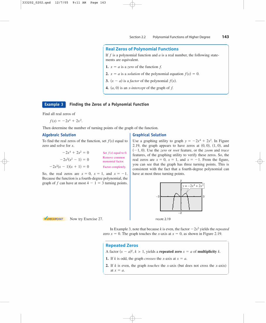
Finding the Zeros of a Polynomial Function

Find all real zeros of

Then determine the number of turning points of the graph of the function.

f (x) � �2x4 � 2x2.

Example 3

Algebraic SolutionTo find the real zeros of the function, set equal tozero and solve for

Set equal to 0.

Factor completely.

So, the real zeros are and Because the function is a fourth-degree polynomial, thegraph of can have at most turning points.


4 � 1 � 3f

x � �1.x � 1,x � 0,

�2x2�x � 1��x � 1� � 0

�2x2�x2 � 1� � 0

f �x� �2x4 � 2x2 � 0

x.f �x�

Graphical SolutionUse a graphing utility to graph In Figure2.19, the graph appears to have zeros at and

Use the zero or root feature, or the zoom and tracefeatures, of the graphing utility to verify these zeros. So, thereal zeros are and From the figure,you can see that the graph has three turning points. This isconsistent with the fact that a fourth-degree polynomial canhave at most three turning points.

FIGURE 2.19

−2

3−3

2

y = −2x4 + 2x2

x � �1.x � 1,x � 0,

��1, 0�.�1, 0�,�0, 0�,

y � �2x4 � 2x2.

In Example 3, note that because is even, the factor yields the repeatedzero The graph touches the -axis at as shown in Figure 2.19.x � 0,xx � 0.

�2x2k

Remove commonmonomial factor.

Repeated ZerosA factor yields a repeated zero of multiplicity

1. If is odd, the graph crosses the -axis at

2. If is even, the graph touches the -axis (but does not cross the -axis)at x � a.

xxk

x � a.xk

k.x � ak > 1,�x � a�k,

333202_0202.qxd 12/7/05 9:11 AM Page 143

To graph polynomial functions, you can use the fact that a polynomialfunction can change signs only at its zeros. Between two consecutive zeros, apolynomial must be entirely positive or entirely negative. This means that whenthe real zeros of a polynomial function are put in order, they divide the realnumber line into intervals in which the function has no sign changes. Theseresulting intervals are test intervals in which a representative -value in theinterval is chosen to determine if the value of the polynomial function is positive(the graph lies above the -axis) or negative (the graph lies below the -axis).

Sketching the Graph of a Polynomial Function

Sketch the graph of

Solution1. Apply the Leading Coefficient Test. Because the leading coefficient is

positive and the degree is even, you know that the graph eventually rises to theleft and to the right (see Figure 2.20).

2. Find the Zeros of the Polynomial. By factoring asyou can see that the zeros of are and (both

of odd multiplicity). So, the -intercepts occur at and Add thesepoints to your graph, as shown in Figure 2.20.

3. Plot a Few Additional Points. Use the zeros of the polynomial to find thetest intervals. In each test interval, choose a representative -value andevaluate the polynomial function, as shown in the table.

4. Draw the Graph. Draw a continuous curve through the points, as shown inFigure 2.21. Because both zeros are of odd multiplicity, you know that thegraph should cross the -axis at and



x

y

−1−2−3−4 2 3 4−1

3

4

5

6

7

f(x) = 3x4 − 4x3

x(0, 0)

Up to rightUp to left

, 043 ))

y

−4 −3 −2 −1 1 2 3 4

7

6

5

4

2

3

−1

x �43.x � 0x

x

�43, 0�.�0, 0�x

x �43x � 0ff �x�� x3�3x � 4�,

f �x� � 3x4 � 4x3

f �x� � 3x4 � 4x3.

xx

x


Example 4 uses an algebraicapproach to describe the graph of the function. A graphing utilityis a complement to this approach.Remember that an importantaspect of using a graphing utilityis to find a viewing window thatshows all significant features of the graph. For instance, theviewing window in part (a) illus-trates all of the significant featuresof the function in Example 4.

a.

b.

Techno logy

−4 5

−3

3

−2 2

−0.5

0.5

Example 4

If you are unsure of the shapeof a portion of the graph of apolynomial function, plot someadditional points, such as thepoint as shownin Figure 2.21.

�0.5, �0.3125�

Test interval Representative Value of f Sign Point onx-value graph

Positive

1 Negative

1.5 Positive �1.5, 1.6875�f �1.5� � 1.6875�43, ��

�1, �1�f �1� � �1�0, 43�

��1, 7�f ��1� � 7�1��, 0�

333202_0202.qxd 12/7/05 9:12 AM Page 144

Sketching the Graph of a Polynomial Function

Sketch the graph of

Solution

1. Apply the Leading Coefficient Test. Because the leading coefficient is nega-tive and the degree is odd, you know that the graph eventually rises to the leftand falls to the right (see Figure 2.22).

2. Find the Zeros of the Polynomial. By factoring

you can see that the zeros of are (odd multiplicity) and (evenmultiplicity). So, the -intercepts occur at and Add these points to your graph, as shown in Figure 2.22.

3. Plot a Few Additional Points. Use the zeros of the polynomial to find the test intervals. In each test interval, choose a representative -value andevaluate the polynomial function, as shown in the table.

4. Draw the Graph. Draw a continuous curve through the points, as shown inFigure 2.23. As indicated by the multiplicities of the zeros, the graph crossesthe -axis at but does not cross the -axis at



1

x−4 −2 −1−3 3 4

f x x x x( ) = 2 + 6− −3 2 92

−2

−1

y

Down to rightUp to left

−2

2

4

6

3

5

x(0, 0)

−4 −2 −1−1

−3 2 31 4

, 032( )

y

�32, 0�.x�0, 0�x

x

�32, 0�.�0, 0�x

x �32x � 0f

� �12x�2x � 3�2

� �12x�4x2 � 12x � 9�

f �x� � �2x3 � 6x2 �92 x

f �x� � �2x3 � 6x2 �92x.


Example 5

Observe in Example 5 that thesign of is positive to theleft of and negative to the rightof the zero Similarly, thesign of is negative to theleft and to the right of the zero

This suggests that if thezero of a polynomial function isof odd multiplicity, then the signof changes from one sideof the zero to the other side. Ifthe zero is of even multiplicity,then the sign of does notchange from one side of thezero to the other side.

f �x�

f �x�

x �32.

f �x�x � 0.

f �x�

Test interval Representative Value of f Sign Point onx-value graph

Positive

0.5 Negative

2 Negative �2, �1�f �2� � �1�32, ��

�0.5, �1�f �0.5� � �1�0, 32�

��0.5, 4�f ��0.5� � 4�0.5��, 0�

333202_0202.qxd 12/7/05 9:12 AM Page 145

The Intermediate Value TheoremThe next theorem, called the Intermediate Value Theorem, illustrates theexistence of real zeros of polynomial functions. This theorem implies that if

and are two points on the graph of a polynomial function suchthat then for any number between and there must be anumber between and such that (See Figure 2.24.)

FIGURE 2.24

The Intermediate Value Theorem helps you locate the real zeros of apolynomial function in the following way. If you can find a value at whicha polynomial function is positive, and another value at which it is nega-tive, you can conclude that the function has at least one real zero between thesetwo values. For example, the function given by is negativewhen and positive when Therefore, it follows from theIntermediate Value Theorem that must have a real zero somewhere between

and as shown in Figure 2.25.

FIGURE 2.25

By continuing this line of reasoning, you can approximate any real zeros ofa polynomial function to any desired accuracy. This concept is further demon-strated in Example 6.

x

f has a zerobetween

2 and 1.− −

f x x x( ) = + + 13 2

( 2, 3)− −

( 1, 1)−

f( 2) = 3− −

f( 1) = 1−

−2 21

−2

−3

−1

y

�1,�2f

x � �1.x � �2f �x� � x3 � x2 � 1

x � bx � a

x

f c d( ) =

f b( )

f a( )

a c b

y

f �c� � d.bacf �b�f �a�df �a� � f �b�,

�b, f �b��a, f �a��


Intermediate Value TheoremLet and be real numbers such that If is a polynomial functionsuch that then, in the interval takes on every valuebetween and f �b�.f �a�

f�a, b�,f �a� � f �b�,fa < b.ba

Activities

1. Find all of the real zeros of

Answer:

2. Determine the right-hand and left-hand behavior of

Answer: The graph rises to the leftand to the right.

3. Find a polynomial function of degree 3 that has zeros of 0, 2,and

Answer: f �x� � 3x3 � 5x2 � 2x

�13.

f�x� � 6x 4 � 33x3 � 18x2.

�12, 0, 6

f�x� � 6x 4 � 33x3 � 18x2.

333202_0202.qxd 12/7/05 9:12 AM Page 146

You can use the table feature of a graphing utility to approximatethe zeros of a polynomial function. For instance, for the functiongiven by

create a table that shows the function values for , asshown in the first table at the right. Scroll through the table lookingfor consecutive function values that differ in sign. From the table,you can see that and differ in sign. So, you can concludefrom the Intermediate Value Theorem that the function has a zerobetween 0 and 1. You can adjust your table to show function valuesfor using increments of 0.1, as shown in the second tableat the right. By scrolling through the table you can see that and differ in sign. So, the function has a zero between 0.8 and 0.9. If you repeat this process several times, you should obtain

as the zero of the function. Use the zero or root feature ofa graphing utility to confirm this result.x � 0.806

f�0.9�f�0.8�

0 ≤ x ≤ 1

f�1�f�0�

�20 ≤ x ≤ 20

f�x� � �2x3 � 3x2 � 3

Techno logy

Approximating a Zero of a Polynomial Function

Use the Intermediate Value Theorem to approximate the real zero of

SolutionBegin by computing a few function values, as follows.

Because is negative and is positive, you can apply the IntermediateValue Theorem to conclude that the function has a zero between and 0. Topinpoint this zero more closely, divide the interval into tenths andevaluate the function at each point. When you do this, you will find that

and

So, must have a zero between and as shown in Figure 2.26. For amore accurate approximation, compute function values between and

and apply the Intermediate Value Theorem again. By continuing thisprocess, you can approximate this zero to any desired accuracy.


f ��0.7�f ��0.8�

�0.7,�0.8f

f ��0.7� � 0.167.f ��0.8� � �0.152

��1, 0��1

f �0�f ��1�

f �x� � x3 � x2 � 1.


The approximation process in Example 6adapts very well to a graphing utility.Have students repeatedly use the zoomand trace features to find that the realzero of occursbetween and �0.754.�0.755

f�x� � x3 � x2 � 1

x

f has a zero

and 0.7.between 0.8−

−

−1 1 2

−1

2

f x x x( ) = + 13 2−

( 1, 1)− −

(0, 1)(1, 1)

y

FIGURE 2.26

x

0 1

1 1

�1�1

�11�2

f �x�

Example 6

333202_0202.qxd 12/7/05 9:12 AM Page 147


Exercises 2.2

In Exercises 1– 8, match the polynomial function with itsgraph. [The graphs are labeled (a), (b), (c), (d), (e), (f ), (g), and(h).]

(a) (b)

(c) (d)

(e) (f)

(g) (h)

1. 2.

3. 4.

5. 6.

7. 8.

In Exercises 9–12, sketch the graph of and eachtransformation.

9.

(a) (b)

(c) (d)

10.

(a) (b)

(c) (d)

11.

(a) (b)

(c) (d)

(e) (f) f�x� � �12 x�4

� 2f�x� � �2x�4 � 1

f �x� �12�x � 1�4f �x� � 4 � x4

f �x� � x4 � 3f �x� � �x � 3�4

y � x4

f �x� � �12�x � 1�5f �x� � 1 �

12x5

f �x� � x5 � 1f �x� � �x � 1�5

y � x5

f �x� � �x � 2�3 � 2f �x� � �12x3

f �x� � x3 � 2f �x� � �x � 2�3

y � x3

y � x n

f �x� �15x5 � 2x3 �

95xf �x� � x4 � 2x3

f �x� � �13x3 � x2 �

43f �x� � �

14x4 � 3x2

f �x� � 2x3 � 3x � 1f �x� � �2x2 � 5x

f �x� � x2 � 4xf �x� � �2x � 3

x2

−4

4

−4−2

y

x62

−4

−2−2

y

x42−4

−4

−2

4

y

x84−8

−8

−4−4

8

y

x42−4

−2

6

4

2

y

x84−8

−8

−4−4

8

4

y

x84−8 −4

8

y

x8−8

−8

−4

y

VOCABULARY CHECK: Fill in the blanks.

1. The graphs of all polynomial functions are ________, which means that the graphs have no breaks, holes, or gaps.

2. The ________ ________ ________ is used to determine the left-hand and right-hand behavior of the graph of a polynomial function.

3. A polynomial function of degree has at most ________ real zeros and at most ________ turning points.

4. If is a zero of a polynomial function then the following three statements are true.

(a) is a ________ of the polynomial equation

(b) ________ is a factor of the polynomial

(c) is an ________ of the graph

5. If a real zero of a polynomial function is of even multiplicity, then the graph of ________ the -axis at and if it is of odd multiplicity then the graph of ________ the -axis at

6. A polynomial function is written in ________ form if its terms are written in descending order of exponents from left to right.

7. The ________ ________ Theorem states that if is a polynomial function such that then in the interval takes on every value between and

PREREQUISITE SKILLS REVIEW: Practice and review algebra skills needed for this section at www.Eduspace.com.

f �b�.f �a�f�a, b�,f �a� � f �b�,f

x � a.xfx � a,xf

f.�a, 0�f �x�.

f �x� � 0.x � a

f,x � a

n

333202_0202.qxd 12/7/05 2:50 PM Page 148


12.

(a) (b)

(c) (d)

(e) (f)

In Exercises 13–22, describe the right-hand and left-handbehavior of the graph of the polynomial function.

13. 14.

15. 16.

17.

18.

19.

20.

21.

22.

Graphical Analysis In Exercises 23–26, use a graphingutility to graph the functions and in the same viewingwindow. Zoom out sufficiently far to show that theright-hand and left-hand behaviors of and appearidentical.

23.

24.

25.

26.

In Exercises 27– 42, (a) find all the real zeros of thepolynomial function, (b) determine the multiplicity of eachzero and the number of turning points of the graph of thefunction, and (c) use a graphing utility to graph thefunction and verify your answers.

27. 28.

29. 30.

31.

32.

33.

34.

35.

36.

37.

38.

39.

40.

41.

42.

Graphical Analysis In Exercises 43–46, (a) use a graphingutility to graph the function, (b) use the graph to approxi-mate any -intercepts of the graph, (c) set and solvethe resulting equation, and (d) compare the results of part(c) with any -intercepts of the graph.

43.

44.

45.

46.

In Exercises 47–56, find a polynomial function that has thegiven zeros. (There are many correct answers.)

47. 48.

49. 50.

51. 52.

53. 54.

55. 56.

In Exercises 57–66, find a polynomial of degree that hasthe given zero(s). (There are many correct answers.)

Zero(s) Degree

57.

58.

59.

60.

61.

62.

63.

64.

65.

66.

In Exercises 67– 80, sketch the graph of the function by (a)applying the Leading Coefficient Test, (b) finding the zerosof the polynomial, (c) plotting sufficient solution points,and (d) drawing a continuous curve through the points.

67. 68.

69.

70.

71. 72.

73.

74.

75. 76.

77. 78.

79.

80. g�x� �110�x � 1�2�x � 3�3

g�t� � �14�t � 2�2�t � 2�2

h�x� �13x3�x � 4�2f �x� � x2�x � 4�

f �x� � �48x2 � 3x4f �x� � �5x2 � x3

f �x� � �4x3 � 4x2 � 15x

f �x� � 3x3 � 15x2 � 18x

f �x� � 1 � x3f �x� � x3 � 3x2

g�x� � �x2 � 10x � 16

f �t� �14�t 2 � 2t � 15�

g�x� � x4 � 4x2f �x� � x3 � 9x

n � 5x � �3, 1, 5, 6

n � 5x � 0, �4

n � 4x � �4, �1, 3, 6

n � 4x � �5, 1, 2

n � 3x � 9

n � 3x � 0, �3, ��3

n � 3x � �2, 4, 7

n � 3x � �3, 0, 1

n � 2x � �8, �4

n � 2x � �2

n

2, 4 � �5, 4 � �51 � �3, 1 ��3

�2, �1, 0, 1, 24, �3, 3, 0

0, 2, 50, �2, �3

�4, 52, �6

0, �30, 10

y �14x3�x2 � 9�

y � x5 � 5x3 � 4x

y � 4x 3 � 4x 2 � 8x � 8

y � 4x3 � 20x2 � 25x

x

y � 0x

f�x� � x3 � 4x2 � 25x � 100

g�x� � x3 � 3x2 � 4x � 12

f�x� � 2x4 � 2x2 � 40

f�x� � 5x4 � 15x2 � 10

f�x� � x5 � x3 � 6x

g�t� � t 5 � 6t 3 � 9t

f�x� � x4 � x3 � 20x2

f �t� � t3 � 4t2 � 4t

g�x� � 5x�x2 � 2x � 1�f�x� � 3x3 � 12x2 � 3x

f �x� �12x2 �

52x �

32

f �x� �13 x2 �

13 x �

23

f�x� � x2 � 10x � 25h�t� � t 2 � 6t � 9

f�x� � 49 � x2f�x� � x2 � 25

g�x� � 3x4f�x� � 3x4 � 6x2,

g�x� � �x4f �x� � ��x4 � 4x3 � 16x�,g�x� � �

13x3f�x� � �

13�x3 � 3x � 2�,

g�x� � 3x3f �x� � 3x3 � 9x � 1,

gf

gf

f�s� � �78�s3 � 5s2 � 7s � 1�

h�t� � �23�t2 � 5t � 3�

f �x� �3x4 � 2x � 5

4

f �x� � 6 � 2x � 4x2 � 5x3

f �x� � 2x5 � 5x � 7.5

f �x� � �2.1x5 � 4x3 � 2

h�x� � 1 � x6g�x� � 5 �72x � 3x2

f �x� � 2x2 � 3x � 1f �x� �13x3 � 5x

f�x� � �2x�6 � 1f�x� � �14 x�6

� 2

f �x� � �14x6 � 1f �x� � x6 � 4

f �x� � �x � 2�6 � 4f �x� � �18x6

y � x6

333202_0202.qxd 12/7/05 9:12 AM Page 149


In Exercises 81–84, use a graphing utility to graph thefunction. Use the zero or root feature to approximate thereal zeros of the function. Then determine the multiplicityof each zero.

81.

82.

83.

84.

In Exercises 85– 88, use the Intermediate Value Theoremand the table feature of a graphing utility to find intervalsone unit in length in which the polynomial function isguaranteed to have a zero. Adjust the table to approximatethe zeros of the function. Use the zero or root feature of agraphing utility to verify your results.

85.

86.

87.

88.

89. Numerical and Graphical Analysis An open boxis to be made from a square piece of material, 36 inches ona side, by cutting equal squares with sides of length fromthe corners and turning up the sides (see figure).

(a) Verify that the volume of the box is given by thefunction

(b) Determine the domain of the function.

(c) Use a graphing utility to create a table that shows thebox height and the corresponding volumes Use thetable to estimate the dimensions that will produce amaximum volume.

(d) Use a graphing utility to graph and use the graph toestimate the value of for which is maximum.Compare your result with that of part (c).

90. Maximum Volume An open box with locking tabs is tobe made from a square piece of material 24 inches on aside. This is to be done by cutting equal squares from thecorners and folding along the dashed lines shown in thefigure.

(a) Verify that the volume of the box is given by thefunction

(b) Determine the domain of the function

(c) Sketch a graph of the function and estimate the value offor which is maximum.

91. Construction A roofing contractor is fabricating guttersfrom 12-inch aluminum sheeting. The contractor plans touse an aluminum siding folding press to create the gutterby creasing equal lengths for the sidewalls (see figure).

(a) Let represent the height of the sidewall of the gutter.Write a function that represents the cross-sectionalarea of the gutter.

(b) The length of the aluminum sheeting is 16 feet. Writea function that represents the volume of one run ofgutter in terms of

(c) Determine the domain of the function in part (b).

(d) Use a graphing utility to create a table that shows thesidewall height and the corresponding volumes Use the table to estimate the dimensions that will pro-duce a maximum volume.

(e) Use a graphing utility to graph Use the graph toestimate the value of for which is a maximum.Compare your result with that of part (d).

(f ) Would the value of change if the aluminum sheetingwere of different lengths? Explain.

x

V�x�xV.

V.x

x.V

Ax

x 12 − 2x x

V�x�x

V.

V�x� � 8x�6 � x��12 � x�.

x x x xx x

24 in

.

24 in.

V�x�xV

V.x

V�x� � x�36 � 2x�2.

x x

x

36 2− x

x

h�x� � x4 � 10x2 � 3

g�x� � 3x4 � 4x3 � 3

f �x� � 0.11x3 � 2.07x2 � 9.81x � 6.88

f �x� � x3 � 3x2 � 3

h�x� �15�x � 2�2�3x � 5�2

g�x� �15�x � 1�2�x � 3��2x � 9�

f �x� �14x4 � 2x2

f �x� � x3 � 4x

333202_0202.qxd 12/7/05 9:12 AM Page 150


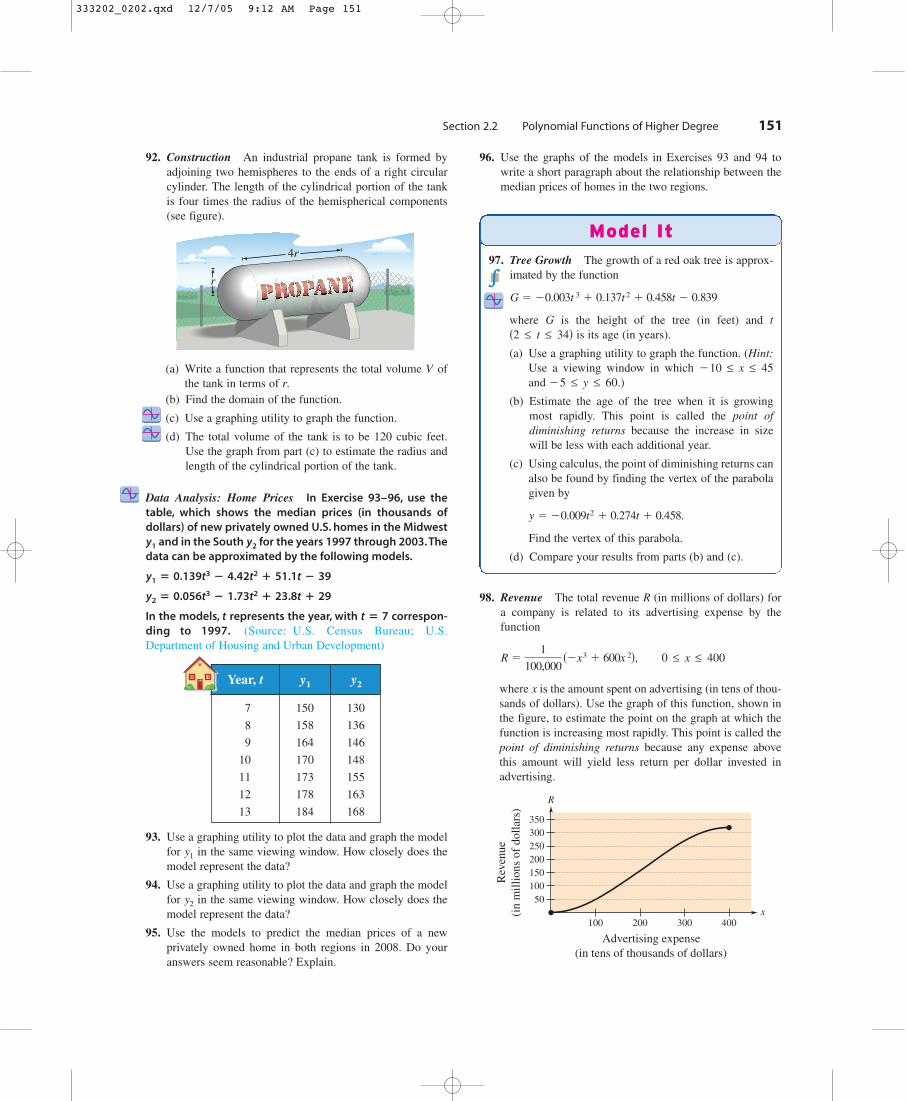
92. Construction An industrial propane tank is formed byadjoining two hemispheres to the ends of a right circularcylinder. The length of the cylindrical portion of the tank is four times the radius of the hemispherical components (see figure).

(a) Write a function that represents the total volume ofthe tank in terms of

(b) Find the domain of the function.

(c) Use a graphing utility to graph the function.

(d) The total volume of the tank is to be 120 cubic feet.Use the graph from part (c) to estimate the radius andlength of the cylindrical portion of the tank.

Data Analysis: Home Prices In Exercise 93–96, use thetable, which shows the median prices (in thousands ofdollars) of new privately owned U.S. homes in the Midwest

and in the South for the years 1997 through 2003.Thedata can be approximated by the following models.

In the models, represents the year, with correspon-ding to 1997. (Source: U.S. Census Bureau; U.S.Department of Housing and Urban Development)

93. Use a graphing utility to plot the data and graph the modelfor in the same viewing window. How closely does themodel represent the data?

94. Use a graphing utility to plot the data and graph the modelfor in the same viewing window. How closely does themodel represent the data?

95. Use the models to predict the median prices of a newprivately owned home in both regions in 2008. Do youranswers seem reasonable? Explain.

96. Use the graphs of the models in Exercises 93 and 94 towrite a short paragraph about the relationship between themedian prices of homes in the two regions.

98. Revenue The total revenue (in millions of dollars) fora company is related to its advertising expense by thefunction

where is the amount spent on advertising (in tens of thou-sands of dollars). Use the graph of this function, shown inthe figure, to estimate the point on the graph at which thefunction is increasing most rapidly. This point is called thepoint of diminishing returns because any expense abovethis amount will yield less return per dollar invested inadvertising.

Advertising expense(in tens of thousands of dollars)

Rev

enue

(in

mill

ions

of

dolla

rs)

x100 200 300 400

100150

50

200250300350

R

x

0 ≤ x ≤ 400R �1

100,000��x3 � 600x 2�,

R

y2

y1

t � 7t

y2 � 0.056t3 � 1.73t2 � 23.8t � 29

y1 � 0.139t3 � 4.42t2 � 51.1t � 39

y2y1

r.V

r

4r

Year, t

7 150 130

8 158 136

9 164 146

10 170 148

11 173 155

12 178 163

13 184 168

y2y1

97. Tree Growth The growth of a red oak tree is approx-imated by the function

where is the height of the tree (in feet) and is its age (in years).

(a) Use a graphing utility to graph the function. (Hint:Use a viewing window in which and

(b) Estimate the age of the tree when it is growingmost rapidly. This point is called the point ofdiminishing returns because the increase in sizewill be less with each additional year.

(c) Using calculus, the point of diminishing returns canalso be found by finding the vertex of the parabolagiven by

Find the vertex of this parabola.

(d) Compare your results from parts (b) and (c).

y � �0.009t2 � 0.274t � 0.458.

�5 ≤ y ≤ 60.)�10 ≤ x ≤ 45

�2 ≤ t ≤ 34�tG

G � �0.003t 3 � 0.137t2 � 0.458t � 0.839

Model It

333202_0202.qxd 12/7/05 9:12 AM Page 151


Synthesis

True or False? In Exercises 99–101, determine whetherthe statement is true or false. Justify your answer.

99. A fifth-degree polynomial can have five turning points inits graph.

100. It is possible for a sixth-degree polynomial to have onlyone solution.

101. The graph of the function given by

rises to the left and falls to the right.

102. Graphical Analysis For each graph, describe a polyno-mial function that could represent the graph. (Indicate thedegree of the function and the sign of its leadingcoefficient.)

(a) (b)

(c) (d)

103. Graphical Reasoning Sketch a graph of the functiongiven by Explain how the graph of eachfunction differs (if it does) from the graph of eachfunction Determine whether is odd, even, or neither.

(a)

(b)

(c)

(d)

(e)

(f )

(g)

(h)

104. Exploration Explore the transformations of the form

(a) Use a graphing utility to graph the functions given by

and

Determine whether the graphs are increasing ordecreasing. Explain.

(b) Will the graph of always be increasing or decreas-ing? If so, is this behavior determined by or Explain.

(c) Use a graphing utility to graph the function given by

Use the graph and the result of part (b) to determinewhether can be written in the form

Explain.

Skills Review

In Exercises 105–108, factor the expression completely.

105. 106.

107. 108.

In Exercises 109 –112, solve the equation by factoring.

109.

110.

111.

112.

In Exercises 113–116, solve the equation by completing thesquare.

113. 114.

115. 116.

In Exercises 117–122, describe the transformation from acommon function that occurs in Then sketch its graph.

117.

118.

119.

120.

121.

122. f �x� � 10 �13�x � 3

f �x� � 2�x � 9

f �x� � 7 � �x � 6

f �x� � �x � 1 � 5

f �x� � 3 � x2

f �x� � �x � 4�2

f x�.

3x2 � 4x � 9 � 02x2 � 5x � 20 � 0

x2 � 8x � 2 � 0x2 � 2x � 21 � 0

x2 � 24x � 144 � 0

12x2 � 11x � 5 � 0

3x2 � 22x � 16 � 0

2x2 � x � 28 � 0

y3 � 2164x4 � 7x3 � 15x2

6x3 � 61x2 � 10x5x2 � 7x � 24

a�x � h�5 � k.H�x� �H

H�x� � x5 � 3x3 � 2x � 1.

k?a, h,g

y2 �3

5�x � 2�5 � 3.

y1 � �1

3�x � 2�5 � 1

g�x� � a�x � h�5 � k.

g�x� � � f � f ��x�g�x� � f �x3�4�g�x� �

12 f �x�

g�x� � f �12x�

g�x� � �f�x�g�x� � f ��x�g�x� � f �x � 2�g�x� � f �x� � 2

gf.g

f �x� � x4.

x

y

x

y

x

y

x

y

f�x� � 2 � x � x2 � x3 � x4 � x5 � x6 � x7

333202_0202.qxd 12/7/05 9:12 AM Page 152

2.2 polynomial functions of higher degree - 2.2...section 2.2 polynomial functions of higher degree...

Documents