21 all pairs shortest path
TRANSCRIPT

Analysis of AlgorithmsAll-Pairs Shortest Path
Andres Mendez-Vazquez
November 11, 2015
1 / 79

Outline1 Introduction
Definition of the ProblemAssumptionsObservations
2 Structure of a Shortest PathIntroduction
3 The SolutionThe Recursive SolutionThe Iterative VersionExtended-Shoertest-PathsLooking at the Algorithm as Matrix MultiplicationExampleWe want something faster
4 A different dynamic-programming algorithmThe Shortest Path StructureThe Bottom-Up SolutionFloyd-Warshall AlgorithmExample
5 Other SolutionsThe Johnson’s Algorithm
6 ExercisesYou can try them
2 / 79

Outline1 Introduction
Definition of the ProblemAssumptionsObservations
2 Structure of a Shortest PathIntroduction
3 The SolutionThe Recursive SolutionThe Iterative VersionExtended-Shoertest-PathsLooking at the Algorithm as Matrix MultiplicationExampleWe want something faster
4 A different dynamic-programming algorithmThe Shortest Path StructureThe Bottom-Up SolutionFloyd-Warshall AlgorithmExample
5 Other SolutionsThe Johnson’s Algorithm
6 ExercisesYou can try them
3 / 79
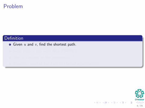
Problem
DefinitionGiven u and v, find the shortest path.Now, what if you want ALL PAIRS!!!Use as a source all the elements in V .Clearly!!! you can fall back to the old algorithms!!!
4 / 79

Problem
DefinitionGiven u and v, find the shortest path.Now, what if you want ALL PAIRS!!!Use as a source all the elements in V .Clearly!!! you can fall back to the old algorithms!!!
4 / 79

Problem
DefinitionGiven u and v, find the shortest path.Now, what if you want ALL PAIRS!!!Use as a source all the elements in V .Clearly!!! you can fall back to the old algorithms!!!
4 / 79

Problem
DefinitionGiven u and v, find the shortest path.Now, what if you want ALL PAIRS!!!Use as a source all the elements in V .Clearly!!! you can fall back to the old algorithms!!!
4 / 79

What can we use?
Use Dijkstra’s |V | times!!!If all the weights are non-negative.This has, using Fibonacci Heaps, O (V 2 log V + VE) complexity.Which is equal O (V 3) in the case of E = O(V 2), but with a hidden largeconstant c.
Use Bellman-Ford |V | times!!!If negative weights are allowed.Then, we have O (V 2E).Which is equal O (V 4) in the case of E = O(V 2).
5 / 79

This is not Good For Large Problems
ProblemsComputer Network Systems.Aircraft Networks (e.g. flying time, fares).Railroad network tables of distances between all pairs of cites for aroad atlas.Etc.
6 / 79

This is not Good For Large Problems
ProblemsComputer Network Systems.Aircraft Networks (e.g. flying time, fares).Railroad network tables of distances between all pairs of cites for aroad atlas.Etc.
6 / 79

This is not Good For Large Problems
ProblemsComputer Network Systems.Aircraft Networks (e.g. flying time, fares).Railroad network tables of distances between all pairs of cites for aroad atlas.Etc.
6 / 79

This is not Good For Large Problems
ProblemsComputer Network Systems.Aircraft Networks (e.g. flying time, fares).Railroad network tables of distances between all pairs of cites for aroad atlas.Etc.
6 / 79

For more on this...Something NotableAs many things in the history of analysis of algorithms the all-pairsshortest path has a long history.
We have more from“Studies in the Economics of Transportation” by Beckmann, McGuire, andWinsten (1956) where the notation that we use for the matrix multiplication alikewas first used.
In additionG. Tarry, Le probleme des labyrinthes, Nouvelles Annales de Mathématiques (3) 14 (1895)187–190 [English translation in: N.L. Biggs, E.K. Lloyd, R.J. Wilson, Graph Theory1736–1936, Clarendon Press, Oxford, 1976, pp. 18–20] (For the theory behinddepth-first search techniques).Chr. Wiener, Ueber eine Aufgabe aus der Geometria situs, Mathematische Annalen 6(1873) 29–30, 1873.
7 / 79

Outline1 Introduction
Definition of the ProblemAssumptionsObservations
2 Structure of a Shortest PathIntroduction
3 The SolutionThe Recursive SolutionThe Iterative VersionExtended-Shoertest-PathsLooking at the Algorithm as Matrix MultiplicationExampleWe want something faster
4 A different dynamic-programming algorithmThe Shortest Path StructureThe Bottom-Up SolutionFloyd-Warshall AlgorithmExample
5 Other SolutionsThe Johnson’s Algorithm
6 ExercisesYou can try them
8 / 79
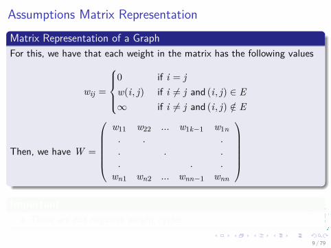
Assumptions Matrix Representation
Matrix Representation of a GraphFor this, we have that each weight in the matrix has the following values
wij =
0 if i = jw(i, j) if i 6= j and (i, j) ∈ E∞ if i 6= j and (i, j) /∈ E
Then, we have W =
w11 w22 ... w1k−1 w1n. . .. . .. . .
wn1 wn2 ... wnn−1 wnn
Important
There are not negative weight cycles.
9 / 79

Outline1 Introduction
Definition of the ProblemAssumptionsObservations
2 Structure of a Shortest PathIntroduction
3 The SolutionThe Recursive SolutionThe Iterative VersionExtended-Shoertest-PathsLooking at the Algorithm as Matrix MultiplicationExampleWe want something faster
4 A different dynamic-programming algorithmThe Shortest Path StructureThe Bottom-Up SolutionFloyd-Warshall AlgorithmExample
5 Other SolutionsThe Johnson’s Algorithm
6 ExercisesYou can try them
10 / 79

Observations
Ah!!!The next algorithm is a dynamic programming algorithm for
I The all-pairs shortest paths problem on a directed graph G = (V ,E).
At the end of the algorithm will generate the following matrix
D =
d11 d22 ... d1k−1 d1n. . .. . .. . .
dn1 dn2 ... dnn−1 dnn
Each entry dij = δ (i, j).
11 / 79

Outline1 Introduction
Definition of the ProblemAssumptionsObservations
2 Structure of a Shortest PathIntroduction
3 The SolutionThe Recursive SolutionThe Iterative VersionExtended-Shoertest-PathsLooking at the Algorithm as Matrix MultiplicationExampleWe want something faster
4 A different dynamic-programming algorithmThe Shortest Path StructureThe Bottom-Up SolutionFloyd-Warshall AlgorithmExample
5 Other SolutionsThe Johnson’s Algorithm
6 ExercisesYou can try them
12 / 79
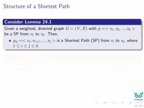
Structure of a Shortest Path
Consider Lemma 24.1Given a weighted, directed graph G = (V ,E) with p =< v1, v2, ..., vk >be a SP from v1 to vk . Then,
pij =< vi , vi+1, ..., vj > is a Shortest Path (SP) from vi to vj , where1 ≤ i ≤ j ≤ k.
We can do the followingConsider the shortest path p from vertex i and j, p contains at mostm edges.Then, we can use the Corollary to make a decomposition
i p′ k → j =⇒ δ(i, j) = δ(i, k) + wkj
13 / 79
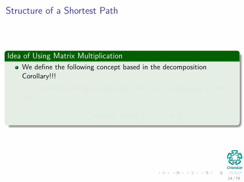
Structure of a Shortest Path
Idea of Using Matrix MultiplicationWe define the following concept based in the decompositionCorollary!!!l(m)ij =minimum weight of any path from i to j, it contains at most medges i.e.
l(m)ij could be min
k
{l(m−1)ik + wkj
}
14 / 79

Structure of a Shortest Path
Idea of Using Matrix MultiplicationWe define the following concept based in the decompositionCorollary!!!l(m)ij =minimum weight of any path from i to j, it contains at most medges i.e.
l(m)ij could be min
k
{l(m−1)ik + wkj
}
14 / 79
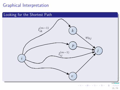
Graphical Interpretation
Looking for the Shortest Path
15 / 79

Outline1 Introduction
Definition of the ProblemAssumptionsObservations
2 Structure of a Shortest PathIntroduction
3 The SolutionThe Recursive SolutionThe Iterative VersionExtended-Shoertest-PathsLooking at the Algorithm as Matrix MultiplicationExampleWe want something faster
4 A different dynamic-programming algorithmThe Shortest Path StructureThe Bottom-Up SolutionFloyd-Warshall AlgorithmExample
5 Other SolutionsThe Johnson’s Algorithm
6 ExercisesYou can try them
16 / 79

Recursive Solution
Thus, we have that for paths with ZERO edges
l(0)ij =
{0 if i = j∞ if i 6= j
Recursion Our Great FriendConsider the previous definition and decomposition. Thus
l(m)ij = min
(l(m−1)ij , min
1≤k≤n
{l(m−1)ik + wkj
})= min
1≤k≤n
{l(m−1)ik + wkj
}
17 / 79

Recursive Solution
Thus, we have that for paths with ZERO edges
l(0)ij =
{0 if i = j∞ if i 6= j
Recursion Our Great FriendConsider the previous definition and decomposition. Thus
l(m)ij = min
(l(m−1)ij , min
1≤k≤n
{l(m−1)ik + wkj
})= min
1≤k≤n
{l(m−1)ik + wkj
}
17 / 79

Recursive Solution
Thus, we have that for paths with ZERO edges
l(0)ij =
{0 if i = j∞ if i 6= j
Recursion Our Great FriendConsider the previous definition and decomposition. Thus
l(m)ij = min
(l(m−1)ij , min
1≤k≤n
{l(m−1)ik + wkj
})= min
1≤k≤n
{l(m−1)ik + wkj
}
17 / 79

Recursive Solution
Thus, we have that for paths with ZERO edges
l(0)ij =
{0 if i = j∞ if i 6= j
Recursion Our Great FriendConsider the previous definition and decomposition. Thus
l(m)ij = min
(l(m−1)ij , min
1≤k≤n
{l(m−1)ik + wkj
})= min
1≤k≤n
{l(m−1)ik + wkj
}
17 / 79

Recursive Solution
Why? A simple notation problem
l(m)ij = l(m−1)
ij + 0 = l(m−1)ij + wjj
18 / 79

Outline1 Introduction
Definition of the ProblemAssumptionsObservations
2 Structure of a Shortest PathIntroduction
3 The SolutionThe Recursive SolutionThe Iterative VersionExtended-Shoertest-PathsLooking at the Algorithm as Matrix MultiplicationExampleWe want something faster
4 A different dynamic-programming algorithmThe Shortest Path StructureThe Bottom-Up SolutionFloyd-Warshall AlgorithmExample
5 Other SolutionsThe Johnson’s Algorithm
6 ExercisesYou can try them
19 / 79

Transforming it to a iterative oneWhat is δ (i, j)?
If you do not have negative-weight cycles, and δ (i, j) <∞.Then, the shortest path from vertex i to j has at most n − 1 edges
δ (i, j) = l(n−1)ij = l(n)
ij = l(n+1)ij = l(n+2)
ij = ...
Back to Matrix MultiplicationWe have the matrix L(m) =
(l(m)ij
).
Then, we can compute first L(1) then compute L(2) all the way toL(n−1) which contains the actual shortest paths.
What is L(1)?First, we have that L(1) = W , since l(1)
ij = wij .
20 / 79

Outline1 Introduction
Definition of the ProblemAssumptionsObservations
2 Structure of a Shortest PathIntroduction
3 The SolutionThe Recursive SolutionThe Iterative VersionExtended-Shoertest-PathsLooking at the Algorithm as Matrix MultiplicationExampleWe want something faster
4 A different dynamic-programming algorithmThe Shortest Path StructureThe Bottom-Up SolutionFloyd-Warshall AlgorithmExample
5 Other SolutionsThe Johnson’s Algorithm
6 ExercisesYou can try them
21 / 79

Algorithm
CodeExtended-Shortest-Path(L,W )
1 n = L.rows2 let L′ =
(l ′ij)be a new n × n
3 for i = 1 to n4 for j = 1 to n5 l ′ij =∞6 for k = 1 to n7 l ′ij = min
(l ′ij , lik + wkj
)8 return L′
22 / 79

Algorithm
CodeExtended-Shortest-Path(L,W )
1 n = L.rows2 let L′ =
(l ′ij)be a new n × n
3 for i = 1 to n4 for j = 1 to n5 l ′ij =∞6 for k = 1 to n7 l ′ij = min
(l ′ij , lik + wkj
)8 return L′
22 / 79

Algorithm
CodeExtended-Shortest-Path(L,W )
1 n = L.rows2 let L′ =
(l ′ij)be a new n × n
3 for i = 1 to n4 for j = 1 to n5 l ′ij =∞6 for k = 1 to n7 l ′ij = min
(l ′ij , lik + wkj
)8 return L′
22 / 79

Algorithm
CodeExtended-Shortest-Path(L,W )
1 n = L.rows2 let L′ =
(l ′ij)be a new n × n
3 for i = 1 to n4 for j = 1 to n5 l ′ij =∞6 for k = 1 to n7 l ′ij = min
(l ′ij , lik + wkj
)8 return L′
22 / 79

Algorithm
ComplexityIf |V | == n we have that Θ
(V 3).
23 / 79

Algorithm
ComplexityIf |V | == n we have that Θ
(V 3).
23 / 79

Outline1 Introduction
Definition of the ProblemAssumptionsObservations
2 Structure of a Shortest PathIntroduction
3 The SolutionThe Recursive SolutionThe Iterative VersionExtended-Shoertest-PathsLooking at the Algorithm as Matrix MultiplicationExampleWe want something faster
4 A different dynamic-programming algorithmThe Shortest Path StructureThe Bottom-Up SolutionFloyd-Warshall AlgorithmExample
5 Other SolutionsThe Johnson’s Algorithm
6 ExercisesYou can try them
24 / 79

Look Alike Matrix Multiplication Operations
Mapping That Can be ThoughtL =⇒ AW =⇒ BL′ =⇒ Cmin =⇒ ++ =⇒ ·∞ =⇒ 0
25 / 79

Look Alike Matrix Multiplication Operations
Using the previous notation, we can rewrite our previous algorithm asSquare-Matrix-Multiply(A,B)
1 n = A.rows2 let C be a new n × n matrix3 for i = 1 to n4 for j = 1 to n5 cij = 06 for k = 1 to n7 cij = cij + aik · bkj8 return C
26 / 79

Complexity
ThusThe complexity of the Extended-Shortest-Path is equal to O
(n3)
27 / 79

Using the Analogy
Returning to the all-pairs shortest-paths problemIt is possible to compute the shortest path by extending such a path edgeby edge.
ThereforeIf we denote A · B as the “product” of the Extended-Shortest-Path
28 / 79

Using the Analogy
Returning to the all-pairs shortest-paths problemIt is possible to compute the shortest path by extending such a path edgeby edge.
ThereforeIf we denote A · B as the “product” of the Extended-Shortest-Path
28 / 79

Using the Analogy
We have that
L(1) = L(0) ·W = WL(2) = L(1) ·W = W 2
...L(n−1) = L(n−2) ·W = W n−1
29 / 79

Using the Analogy
We have that
L(1) = L(0) ·W = WL(2) = L(1) ·W = W 2
...L(n−1) = L(n−2) ·W = W n−1
29 / 79

Using the Analogy
We have that
L(1) = L(0) ·W = WL(2) = L(1) ·W = W 2
...L(n−1) = L(n−2) ·W = W n−1
29 / 79

The Final Algorithm
We have thatSlow-All-Pairs-Shortest-Paths(W )
1 n ←W .rows2 L(1) ←W3 for m = 2 to n − 14 L(m) ←EXTEND-SHORTEST-PATHS
(L(m−1),W
)5 return L(n−1)
30 / 79

With Complexity
Complexity
O(V 4)
(1)
31 / 79

Outline1 Introduction
Definition of the ProblemAssumptionsObservations
2 Structure of a Shortest PathIntroduction
3 The SolutionThe Recursive SolutionThe Iterative VersionExtended-Shoertest-PathsLooking at the Algorithm as Matrix MultiplicationExampleWe want something faster
4 A different dynamic-programming algorithmThe Shortest Path StructureThe Bottom-Up SolutionFloyd-Warshall AlgorithmExample
5 Other SolutionsThe Johnson’s Algorithm
6 ExercisesYou can try them
32 / 79

ExampleWe have the following
1
2
3
45
3 4
8
2
7
1
6
-4-5
1 2 3 4 51 0 2 8 ∞ -42 ∞ 0 ∞ 1 73 ∞ 4 0 ∞ ∞4 2 ∞ -5 0 ∞5 ∞ ∞ ∞ 6 0
L(1) = L(0)W
33 / 79

ExampleWe have the following
1
2
3
45
3 4
8
2
7
1
6
-4-5
1 2 3 4 51 0 2 8 2 -42 3 0 -4 1 73 ∞ 4 0 5 114 2 -1 -5 0 -25 8 ∞ 1 6 0
L(2) = L(1)W
34 / 79
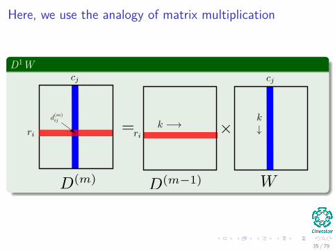
Here, we use the analogy of matrix multiplication
D1W
35 / 79

Thus, the update of an element lij
Example
l(2)14 = min
(
0 3 8 ∞ −4)
+
∞1∞06
= min
(∞ 4 ∞ ∞ 2
)= 2
36 / 79

ExampleWe have the following
1
2
3
45
3 4
8
2
7
1
6
-4-5
1 2 3 4 51 0 3 -3 2 -42 3 0 -4 1 -13 7 4 0 5 114 2 -1 -5 0 -25 8 5 1 6 0
L(3) = L(2)W
37 / 79

ExampleWe have the following
1
2
3
45
3 4
8
2
7
1
6
-4-5
1 2 3 4 51 0 1 -3 2 -42 3 0 -4 1 -13 7 4 0 5 34 2 -1 -5 0 -25 8 5 1 6 0
L(4) = L(3)W
38 / 79

Outline1 Introduction
Definition of the ProblemAssumptionsObservations
2 Structure of a Shortest PathIntroduction
3 The SolutionThe Recursive SolutionThe Iterative VersionExtended-Shoertest-PathsLooking at the Algorithm as Matrix MultiplicationExampleWe want something faster
4 A different dynamic-programming algorithmThe Shortest Path StructureThe Bottom-Up SolutionFloyd-Warshall AlgorithmExample
5 Other SolutionsThe Johnson’s Algorithm
6 ExercisesYou can try them
39 / 79

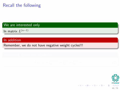
Recall the following
We are interested onlyIn matrix L(n−1)
In additionRemember, we do not have negative weight cycles!!!
Therefore, given the equation
δ (i, j) = l(n−1)ij = l(n)
ij = l(n)ij = ... (2)
40 / 79
Recall the following
We are interested onlyIn matrix L(n−1)
In additionRemember, we do not have negative weight cycles!!!
Therefore, given the equation
δ (i, j) = l(n−1)ij = l(n)
ij = l(n)ij = ... (2)
40 / 79

Recall the following
We are interested onlyIn matrix L(n−1)
In additionRemember, we do not have negative weight cycles!!!
Therefore, given the equation
δ (i, j) = l(n−1)ij = l(n)
ij = l(n)ij = ... (2)
40 / 79

Thus
It implies
L(m) = L(n−1) (3)
For all
m ≥ n − 1 (4)
41 / 79

Thus
It implies
L(m) = L(n−1) (3)
For all
m ≥ n − 1 (4)
41 / 79

Something Faster
We want something faster!!! Observation!!!
L(1) = WL(2) = W ·W = W 2
L(4) = W 2 ·W 2 = W 4
L(8) = W 4 ·W 4 = W 8
...L(2dlog(n−1)e) = W d2dlog(n−1)e−1e ·W 2dlog(n−1)e−1 = W 2dlog(n−1)e
Because
2dlg(n−1)e ≥ n − 1 =⇒ L(2dlg(n−1)e) = L(n−1)
42 / 79

Something Faster
We want something faster!!! Observation!!!
L(1) = WL(2) = W ·W = W 2
L(4) = W 2 ·W 2 = W 4
L(8) = W 4 ·W 4 = W 8
...L(2dlog(n−1)e) = W d2dlog(n−1)e−1e ·W 2dlog(n−1)e−1 = W 2dlog(n−1)e
Because
2dlg(n−1)e ≥ n − 1 =⇒ L(2dlg(n−1)e) = L(n−1)
42 / 79

Something Faster
We want something faster!!! Observation!!!
L(1) = WL(2) = W ·W = W 2
L(4) = W 2 ·W 2 = W 4
L(8) = W 4 ·W 4 = W 8
...L(2dlog(n−1)e) = W d2dlog(n−1)e−1e ·W 2dlog(n−1)e−1 = W 2dlog(n−1)e
Because
2dlg(n−1)e ≥ n − 1 =⇒ L(2dlg(n−1)e) = L(n−1)
42 / 79

Something Faster
We want something faster!!! Observation!!!
L(1) = WL(2) = W ·W = W 2
L(4) = W 2 ·W 2 = W 4
L(8) = W 4 ·W 4 = W 8
...L(2dlog(n−1)e) = W d2dlog(n−1)e−1e ·W 2dlog(n−1)e−1 = W 2dlog(n−1)e
Because
2dlg(n−1)e ≥ n − 1 =⇒ L(2dlg(n−1)e) = L(n−1)
42 / 79

Something Faster
We want something faster!!! Observation!!!
L(1) = WL(2) = W ·W = W 2
L(4) = W 2 ·W 2 = W 4
L(8) = W 4 ·W 4 = W 8
...L(2dlog(n−1)e) = W d2dlog(n−1)e−1e ·W 2dlog(n−1)e−1 = W 2dlog(n−1)e
Because
2dlg(n−1)e ≥ n − 1 =⇒ L(2dlg(n−1)e) = L(n−1)
42 / 79

Something Faster
We want something faster!!! Observation!!!
L(1) = WL(2) = W ·W = W 2
L(4) = W 2 ·W 2 = W 4
L(8) = W 4 ·W 4 = W 8
...L(2dlog(n−1)e) = W d2dlog(n−1)e−1e ·W 2dlog(n−1)e−1 = W 2dlog(n−1)e
Because
2dlg(n−1)e ≥ n − 1 =⇒ L(2dlg(n−1)e) = L(n−1)
42 / 79

The Faster Algorithm
Complexity of the Previous AlgorithmSlow-All-Pairs-Shortest-Paths(W )
1 n ←W .rows2 L(1) ←W3 m ← 14 while m < n − 15 L(2m) ←EXTEND-SHORTEST-PATHS
(L(m),L(m)
)6 m ← 2m7 return L(m)
ComplexityIf n = |V | we have that O
(V 3 lg V
).
43 / 79

The Faster Algorithm
Complexity of the Previous AlgorithmSlow-All-Pairs-Shortest-Paths(W )
1 n ←W .rows2 L(1) ←W3 m ← 14 while m < n − 15 L(2m) ←EXTEND-SHORTEST-PATHS
(L(m),L(m)
)6 m ← 2m7 return L(m)
ComplexityIf n = |V | we have that O
(V 3 lg V
).
43 / 79

Outline1 Introduction
Definition of the ProblemAssumptionsObservations
2 Structure of a Shortest PathIntroduction
3 The SolutionThe Recursive SolutionThe Iterative VersionExtended-Shoertest-PathsLooking at the Algorithm as Matrix MultiplicationExampleWe want something faster
4 A different dynamic-programming algorithmThe Shortest Path StructureThe Bottom-Up SolutionFloyd-Warshall AlgorithmExample
5 Other SolutionsThe Johnson’s Algorithm
6 ExercisesYou can try them
44 / 79

The Shortest Path Structure
Intermediate VertexFor a path p = 〈v1, v2, ..., vl〉, an intermediate vertex is any vertex of pother than v1 or vl .
Defined(k)
ij =weight of a shortest path between i and j with all intermediatevertices are in the set {1, 2, ..., k}.
45 / 79

The Shortest Path Structure
Intermediate VertexFor a path p = 〈v1, v2, ..., vl〉, an intermediate vertex is any vertex of pother than v1 or vl .
Defined(k)
ij =weight of a shortest path between i and j with all intermediatevertices are in the set {1, 2, ..., k}.
45 / 79

The Recursive IdeaSimply look at the following cases cases
Case I k is not an intermediate vertex, then a shortest path from i toj with all intermediate vertices {1, ..., k − 1} is a shortest path from ito j with intermediate vertices {1, ..., k}.
=⇒ d(k)ij = d(k−1)
ij
Case II if k is an intermediate vertice. Then, i p1 k p2 j and we canmake the following statements using Lemma 24.1:
I p1 is a shortest path from i to k with all intermediate vertices in theset {1, ..., k − 1}.
I p2 is a shortest path from k to j with all intermediate vertices in theset {1, ..., k − 1}.
=⇒ d(k)ij = d(k−1)
ik + d(k−1)kj
46 / 79

The Graphical Idea
ConsiderAll possible intermediate vertices in {1, 2, ..., k}
Figure: The Recursive Idea
47 / 79

The Recursive Solution
The Recursion
d(k)ij =
wij if k = 0min
(d(k−1)
ij , d(k−1)ik + d(k−1)
kj
)if k ≥ 1
Final answer when k = nWe recursively calculate D(n) =
(d(n)
ij
)or d(n)
ij = δ (i, j) for all i, j ∈ V .
48 / 79

The Recursive Solution
The Recursion
d(k)ij =
wij if k = 0min
(d(k−1)
ij , d(k−1)ik + d(k−1)
kj
)if k ≥ 1
Final answer when k = nWe recursively calculate D(n) =
(d(n)
ij
)or d(n)
ij = δ (i, j) for all i, j ∈ V .
48 / 79

Thus, we have the following
Recursive VersionRecursive-Floyd-Warshall(W )
1 D(n) the n × n matrix2 for i = 1 to n3 for j = 1 to n4 D(n) [i, j] =Recursive-Part(i, j, n,W )5 return D(n)
49 / 79

Thus, we have the following
Recursive VersionRecursive-Floyd-Warshall(W )
1 D(n) the n × n matrix2 for i = 1 to n3 for j = 1 to n4 D(n) [i, j] =Recursive-Part(i, j, n,W )5 return D(n)
49 / 79
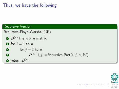
Thus, we have the following
Recursive VersionRecursive-Floyd-Warshall(W )
1 D(n) the n × n matrix2 for i = 1 to n3 for j = 1 to n4 D(n) [i, j] =Recursive-Part(i, j, n,W )5 return D(n)
49 / 79

Thus, we have the following
The Recursive-PartRecursive-Part(i, j, k,W )
1 if k = 02 return W [i, j]3 if k ≥ 14 t1 =Recursive-Part(i, j, k − 1,W )5 t2 =Recursive-Part(i, k, k − 1,W )+...6 Recursive-Part(k, j, k − 1,W )7 if t1 ≤ t28 return t19 else10 return t2
50 / 79

Thus, we have the following
The Recursive-PartRecursive-Part(i, j, k,W )
1 if k = 02 return W [i, j]3 if k ≥ 14 t1 =Recursive-Part(i, j, k − 1,W )5 t2 =Recursive-Part(i, k, k − 1,W )+...6 Recursive-Part(k, j, k − 1,W )7 if t1 ≤ t28 return t19 else10 return t2
50 / 79

Thus, we have the following
The Recursive-PartRecursive-Part(i, j, k,W )
1 if k = 02 return W [i, j]3 if k ≥ 14 t1 =Recursive-Part(i, j, k − 1,W )5 t2 =Recursive-Part(i, k, k − 1,W )+...6 Recursive-Part(k, j, k − 1,W )7 if t1 ≤ t28 return t19 else10 return t2
50 / 79

Thus, we have the following
The Recursive-PartRecursive-Part(i, j, k,W )
1 if k = 02 return W [i, j]3 if k ≥ 14 t1 =Recursive-Part(i, j, k − 1,W )5 t2 =Recursive-Part(i, k, k − 1,W )+...6 Recursive-Part(k, j, k − 1,W )7 if t1 ≤ t28 return t19 else10 return t2
50 / 79

Outline1 Introduction
Definition of the ProblemAssumptionsObservations
2 Structure of a Shortest PathIntroduction
3 The SolutionThe Recursive SolutionThe Iterative VersionExtended-Shoertest-PathsLooking at the Algorithm as Matrix MultiplicationExampleWe want something faster
4 A different dynamic-programming algorithmThe Shortest Path StructureThe Bottom-Up SolutionFloyd-Warshall AlgorithmExample
5 Other SolutionsThe Johnson’s Algorithm
6 ExercisesYou can try them
51 / 79

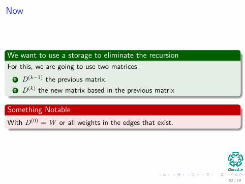
Now
We want to use a storage to eliminate the recursionFor this, we are going to use two matrices
1 D(k−1) the previous matrix.2 D(k) the new matrix based in the previous matrix
Something NotableWith D(0) = W or all weights in the edges that exist.
52 / 79

Now
We want to use a storage to eliminate the recursionFor this, we are going to use two matrices
1 D(k−1) the previous matrix.2 D(k) the new matrix based in the previous matrix
Something NotableWith D(0) = W or all weights in the edges that exist.
52 / 79

Now
We want to use a storage to eliminate the recursionFor this, we are going to use two matrices
1 D(k−1) the previous matrix.2 D(k) the new matrix based in the previous matrix
Something NotableWith D(0) = W or all weights in the edges that exist.
52 / 79
Now
We want to use a storage to eliminate the recursionFor this, we are going to use two matrices
1 D(k−1) the previous matrix.2 D(k) the new matrix based in the previous matrix
Something NotableWith D(0) = W or all weights in the edges that exist.
52 / 79

In addition, we want to rebuild the answer
For this, we have the predecessor matrix ΠActually, we want to compute a sequence of matrices
Π(0),Π(1), ...,Π(n)
Where
Π = Π(n)
53 / 79

In addition, we want to rebuild the answer
For this, we have the predecessor matrix ΠActually, we want to compute a sequence of matrices
Π(0),Π(1), ...,Π(n)
Where
Π = Π(n)
53 / 79
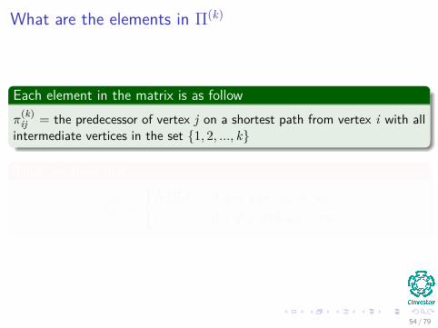
What are the elements in Π(k)
Each element in the matrix is as followπ
(k)ij = the predecessor of vertex j on a shortest path from vertex i with all
intermediate vertices in the set {1, 2, ..., k}
Thus, we have that
π(0)ij =
NULL if i = j or wij =∞i if i 6= j and wij <∞
54 / 79

What are the elements in Π(k)
Each element in the matrix is as followπ
(k)ij = the predecessor of vertex j on a shortest path from vertex i with all
intermediate vertices in the set {1, 2, ..., k}
Thus, we have that
π(0)ij =
NULL if i = j or wij =∞i if i 6= j and wij <∞
54 / 79

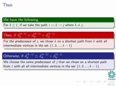
Then
We have the followingFor k ≥ 1, if we take the path i k j where k 6= j.
Then, if d(k−1)ij > d(k−1)
ik + d(k−1)kj
For the predecessor of j, we chose k on a shortest path from k with allintermediate vertices in the set {1, 2, ..., k − 1}
Otherwise, if d(k−1)ij ≤ d(k−1)
ik + d(k−1)kj
We choose the same predecessor of j that we chose on a shortest pathfrom i with all all intermediate vertices in the set {1, 2, ..., k − 1}.
55 / 79

Formally
We have then
π(k)ij =
π(k−1)ij if d(k−1)
ij ≤ d(k−1)ik + d(k−1)
kj
π(k−1)kj if d(k−1)
ij > d(k−1)ik + d(k−1)
kj
56 / 79

Outline1 Introduction
Definition of the ProblemAssumptionsObservations
2 Structure of a Shortest PathIntroduction
3 The SolutionThe Recursive SolutionThe Iterative VersionExtended-Shoertest-PathsLooking at the Algorithm as Matrix MultiplicationExampleWe want something faster
4 A different dynamic-programming algorithmThe Shortest Path StructureThe Bottom-Up SolutionFloyd-Warshall AlgorithmExample
5 Other SolutionsThe Johnson’s Algorithm
6 ExercisesYou can try them
57 / 79

Final Iterative Version of Floyd-Warshall (Correction by Diego - Class Tec 2015)
Floyd-Warshall(W )
1. n = W .rows
2. D(0) = W3. for k = 1 to n − 1
4. let D(k) =(
d(k)ij
)be a newn × n matrix
5. let Π(k) be a newpredecessor
n × n matrix
. Given each k, we update using D(k−1)
6. for i = 1 to n7. for j = 1 to n
8. if d(k−1)ij ≤ d(k−1)
ik + d(k−1)kj
9. d(k)ij = d(k−1)
ij
10. π(k)ij = π
(k−1)ij
11. else12. d(k)
ij = d(k−1)ik + d(k−1)
kj
13. π(k)ij = π
(k−1)kj
14. return D(n) and Π(n)
58 / 79

Explanation
Lines 1 and 2Initialization of variables n and D(0)
Line 3In the loop, we solve the smaller problems first with k = 1 to k = n − 1
Remember the largest number of edges in any shortest path
Line 4 and 5Instantiation of the new matrices D(k) and
∏(k) to generate the shortestpats with at least k edges.
59 / 79

Explanation
Line 6 and 7This is done to go through all the possible combinations of i’s and j’s
Line 8Deciding if d(k−1)
ij ≤ d(k−1)ik + d(k−1)
kj
60 / 79

Explanation
Line 6 and 7This is done to go through all the possible combinations of i’s and j’s
Line 8Deciding if d(k−1)
ij ≤ d(k−1)ik + d(k−1)
kj
60 / 79

Example
Graph
1
2
3
45
3 4
8
2
7
1
6
-4-5
61 / 79

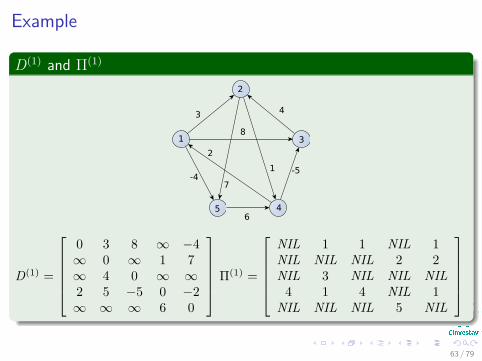
Example
D(0) and Π(0)
1
2
3
45
3 4
8
2
7
1
6
-4-5
D(0) =
0 3 8 ∞ −4∞ 0 ∞ 1 7∞ 4 0 ∞ ∞2 ∞ −5 0 ∞∞ ∞ ∞ 6 0
Π(0) =
NIL 1 1 NIL 1NIL NIL NIL 2 2NIL 3 NIL NIL NIL
4 NIL 4 NIL NILNIL NIL NIL 5 NIL
62 / 79
Example
D(1) and Π(1)
1
2
3
45
3 4
8
2
7
1
6
-4-5
D(1) =
0 3 8 ∞ −4∞ 0 ∞ 1 7∞ 4 0 ∞ ∞2 5 −5 0 −2∞ ∞ ∞ 6 0
Π(1) =
NIL 1 1 NIL 1NIL NIL NIL 2 2NIL 3 NIL NIL NIL
4 1 4 NIL 1NIL NIL NIL 5 NIL
63 / 79
Example
D(2) and Π(2)
1
2
3
45
3 4
8
2
7
1
6
-4-5
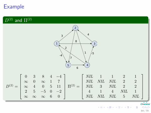
D(2) =
0 3 8 4 −4∞ 0 ∞ 1 7∞ 4 0 5 112 5 −5 0 −2∞ ∞ ∞ 6 0
Π(2) =
NIL 1 1 2 1NIL NIL NIL 2 2NIL 3 NIL 2 2
4 1 4 NIL 1NIL NIL NIL 5 NIL
64 / 79

Example
D(3) and Π(3)
1
2
3
45
3 4
8
2
7
1
6
-4-5
D(3) =
0 3 8 4 −4∞ 0 ∞ 1 7∞ 4 0 5 112 −1 −5 0 −2∞ ∞ ∞ 6 0
Π(3) =
NIL 1 1 2 1NIL NIL NIL 2 2NIL 3 NIL 2 2
4 3 4 NIL 1NIL NIL NIL 5 NIL
65 / 79
Example
D(4) and Π(4)
1
2
3
45
3 4
8
2
7
1
6
-4-5
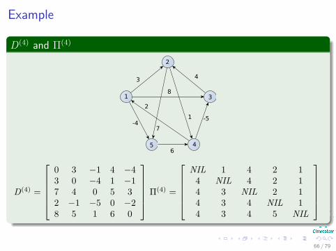
D(4) =
0 3 −1 4 −43 0 −4 1 −17 4 0 5 32 −1 −5 0 −28 5 1 6 0
Π(4) =
NIL 1 4 2 1
4 NIL 4 2 14 3 NIL 2 14 3 4 NIL 14 3 4 5 NIL
66 / 79

Example
D(5) and Π(5)
1
2
3
45
3 4
8
2
7
1
6
-4-5
D(5) =
0 1 −3 2 −43 0 −4 1 −17 4 0 5 32 −1 −5 0 −28 5 1 6 0
Π(5) =
NIL 3 4 5 1
4 NIL 4 2 14 3 NIL 2 14 3 4 NIL 14 3 4 5 NIL
67 / 79

Remarks
Something NotableBecause the comparison in line 8 takes O (1)
Complexity of Floyd-Warshall isTime Complexity Θ
(V 3)
We do not have elaborate data structures as Binary Heap orFibonacci Heap!!!The hidden constant time is quite small:
Making the Floyd-Warshall Algorithm practical even withmoderate-sized graphs!!!
68 / 79

Outline1 Introduction
Definition of the ProblemAssumptionsObservations
2 Structure of a Shortest PathIntroduction
3 The SolutionThe Recursive SolutionThe Iterative VersionExtended-Shoertest-PathsLooking at the Algorithm as Matrix MultiplicationExampleWe want something faster
4 A different dynamic-programming algorithmThe Shortest Path StructureThe Bottom-Up SolutionFloyd-Warshall AlgorithmExample
5 Other SolutionsThe Johnson’s Algorithm
6 ExercisesYou can try them
69 / 79
Johnson’s AlgorithmObservations
Used to find all pairs in a sparse graphs by using Dijkstra’s algorithm.It uses a re-weighting function to obtain positive edges from negativeedges to deal with them.It can deal with the negative weight cycles.
TherforeIt uses something to deal with the negative weight cycles.
I Could be a Bellman-Ford detector as before?
Maybe, we need to transform the weights in order to use them.
What we requireA re-weighting function w (u, v)
I A shortest path by w is a shortest path by w.I All edges are not negative using w.
70 / 79

Proving Properties of Re-Weigthing
Lemma 25.1Given a weighted, directed graph G = (D,V ) with weight functionw : E → R, let h : V → R be any function mapping vertices to realnumbers. For each edge (u, v) ∈ E , define
w (u, v) = w (u, v) + h (u)− h (v)
Let p = 〈v0, v1, ..., vk〉 be any path from vertex 0 to vertex k. Then:1 p is a shortest path from 0 to k with weight function w if and only if
it is a shortest path with weight function w. That is w(p) = δ (v0, vk)if and only if w(p) = δ (v0, vk).
2 Furthermore, G has a negative-weight cycle using weight function wif and only if G has a negative-weight cycle using weight function w.
71 / 79
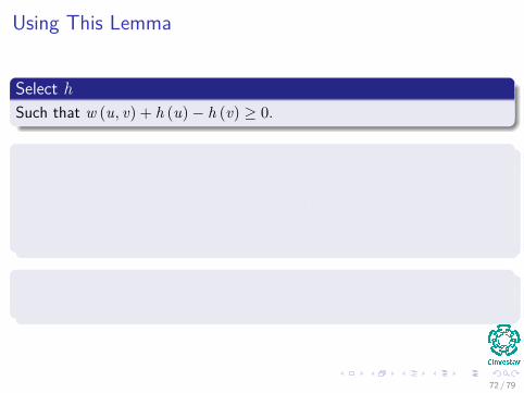
Using This Lemma
Select hSuch that w (u, v) + h (u)− h (v) ≥ 0.
Then, we build a new graph G ′
It has the following elementsI V ′ = V ∪ {s}, where s is a new vertex.I E ′ = E ∪ {(s, v) |v ∈ V }.I w(s, v) = 0 for all v ∈ V , in addition to all the other weights.
Select hSimply select h(v) = δ(s, v).
72 / 79

Example
Graph G ′ with original weight function w with new source s andh(v) = δ(s, v) at each vertex
0
0 0
0
0
0
0
-1
1
2
3
4
5
-4
7
34
8
2
1
6
s -5
-5
-4 0
73 / 79
Proof of Claim
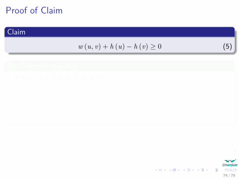
Claim
w (u, v) + h (u)− h (v) ≥ 0 (5)
By Triangle Inequalityδ (s, v) ≤ δ(s, u) + w(u, v)Then by the way we selected h, we have:
h(v) ≤ h(u) + w (u, v) (6)
Finally
w (u, v) + h (u)− h (v) ≥ 0 (7)
74 / 79

Proof of Claim
Claim
w (u, v) + h (u)− h (v) ≥ 0 (5)
By Triangle Inequalityδ (s, v) ≤ δ(s, u) + w(u, v)Then by the way we selected h, we have:
h(v) ≤ h(u) + w (u, v) (6)
Finally
w (u, v) + h (u)− h (v) ≥ 0 (7)
74 / 79

Proof of Claim
Claim
w (u, v) + h (u)− h (v) ≥ 0 (5)
By Triangle Inequalityδ (s, v) ≤ δ(s, u) + w(u, v)Then by the way we selected h, we have:
h(v) ≤ h(u) + w (u, v) (6)
Finally
w (u, v) + h (u)− h (v) ≥ 0 (7)
74 / 79

Proof of Claim
Claim
w (u, v) + h (u)− h (v) ≥ 0 (5)
By Triangle Inequalityδ (s, v) ≤ δ(s, u) + w(u, v)Then by the way we selected h, we have:
h(v) ≤ h(u) + w (u, v) (6)
Finally
w (u, v) + h (u)− h (v) ≥ 0 (7)
74 / 79

Example
The new Graph G after re-weighting G ′
0
5 1
0
4
0
0
-1
1
2
3
4
5
0
10
40
13
2
0
2
s 0
-5
-4 0
75 / 79

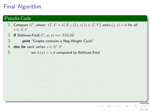
Final Algorithm
Pseudo-Code1. Compute G′, where: G′.V = G.E ∪ {(s, v) |v ∈ G.V} andw (s, v) = 0 for all
v ∈ G.V2. If Bellman-Ford(G′,w, s) == FALSE3. print “Graphs contains a Neg-Weight Cycle”4. else for each vertex v ∈ G′.V5. set h (v) = v.d computed by Bellman-Ford6. for each edge (u, v) ∈ G′.E7. w (u, v) = w (u, v) + h (u)− h (v)8. Let D = (duv) be a new n × n matrix9. for each vertex u ∈ G.V10. run Dijkstra(G, w, u) to compute δ (u, v) for all v ∈ G.V11. for each vertex v ∈ G.V12. duv = δ (u, v) + h (v)− h (u)13. return D
76 / 79

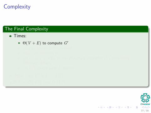
Complexity
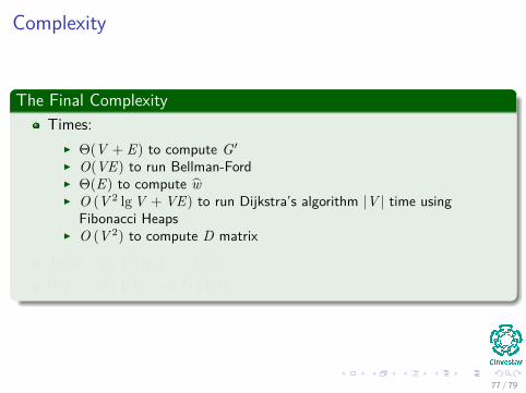
The Final ComplexityTimes:
I Θ(V + E) to compute G′I O(VE) to run Bellman-FordI Θ(E) to compute wI O (V 2 lg V + VE) to run Dijkstra’s algorithm |V | time using
Fibonacci HeapsI O (V 2) to compute D matrix
Total : O(V 2 lg V + VE)If E = O
(V 2) =⇒ O
(V 3)
77 / 79
Complexity
The Final ComplexityTimes:
I Θ(V + E) to compute G′I O(VE) to run Bellman-FordI Θ(E) to compute wI O (V 2 lg V + VE) to run Dijkstra’s algorithm |V | time using
Fibonacci HeapsI O (V 2) to compute D matrix
Total : O(V 2 lg V + VE)If E = O
(V 2) =⇒ O
(V 3)
77 / 79

Complexity
The Final ComplexityTimes:
I Θ(V + E) to compute G′I O(VE) to run Bellman-FordI Θ(E) to compute wI O (V 2 lg V + VE) to run Dijkstra’s algorithm |V | time using
Fibonacci HeapsI O (V 2) to compute D matrix
Total : O(V 2 lg V + VE)If E = O
(V 2) =⇒ O
(V 3)
77 / 79

Complexity
The Final ComplexityTimes:
I Θ(V + E) to compute G′I O(VE) to run Bellman-FordI Θ(E) to compute wI O (V 2 lg V + VE) to run Dijkstra’s algorithm |V | time using
Fibonacci HeapsI O (V 2) to compute D matrix
Total : O(V 2 lg V + VE)If E = O
(V 2) =⇒ O
(V 3)
77 / 79

Complexity
The Final ComplexityTimes:
I Θ(V + E) to compute G′I O(VE) to run Bellman-FordI Θ(E) to compute wI O (V 2 lg V + VE) to run Dijkstra’s algorithm |V | time using
Fibonacci HeapsI O (V 2) to compute D matrix
Total : O(V 2 lg V + VE)If E = O
(V 2) =⇒ O
(V 3)
77 / 79
Complexity
The Final ComplexityTimes:
I Θ(V + E) to compute G′I O(VE) to run Bellman-FordI Θ(E) to compute wI O (V 2 lg V + VE) to run Dijkstra’s algorithm |V | time using
Fibonacci HeapsI O (V 2) to compute D matrix
Total : O(V 2 lg V + VE)If E = O
(V 2) =⇒ O
(V 3)
77 / 79

Complexity
The Final ComplexityTimes:
I Θ(V + E) to compute G′I O(VE) to run Bellman-FordI Θ(E) to compute wI O (V 2 lg V + VE) to run Dijkstra’s algorithm |V | time using
Fibonacci HeapsI O (V 2) to compute D matrix
Total : O(V 2 lg V + VE)If E = O
(V 2) =⇒ O
(V 3)
77 / 79

Complexity
The Final ComplexityTimes:
I Θ(V + E) to compute G′I O(VE) to run Bellman-FordI Θ(E) to compute wI O (V 2 lg V + VE) to run Dijkstra’s algorithm |V | time using
Fibonacci HeapsI O (V 2) to compute D matrix
Total : O(V 2 lg V + VE)If E = O
(V 2) =⇒ O
(V 3)
77 / 79

Outline1 Introduction
Definition of the ProblemAssumptionsObservations
2 Structure of a Shortest PathIntroduction
3 The SolutionThe Recursive SolutionThe Iterative VersionExtended-Shoertest-PathsLooking at the Algorithm as Matrix MultiplicationExampleWe want something faster
4 A different dynamic-programming algorithmThe Shortest Path StructureThe Bottom-Up SolutionFloyd-Warshall AlgorithmExample
5 Other SolutionsThe Johnson’s Algorithm
6 ExercisesYou can try them
78 / 79

Excercises
25.1-425.1-825.1-925.2-425.2-625.2-925.3-3
79 / 79