2025-44 satellite navigation science and technology for...
TRANSCRIPT

2025-44
Satellite Navigation Science and Technology for Africa
LANGLEY Richard B.
23 March - 9 April, 2009
University of New BrunswickGeodetic Research Laboratory
Geodesy and Geomatics EngineeringFredericton N.B., E3B 5A3
CANADA
Atmospheric Monitoring and Mitigation

© Richard B. Langley, 2009 1
Atmospheric Mitigation and Monitoring
Richard B. LangleyDept. of Geodesy and Geomatics Engineering
University of New BrunswickFredericton, NB E3B5A3, Canada
Satellite Navigation Science and Technology for AfricaInternational Centre for Theoretical Physics, Trieste, Italy
23 March – 9 April, 2009

© Richard B. Langley, 2009 2
Motivation-1
80 km
50 km
9-16 km
Ionosphere
Stratosphere
Tropopause
Troposphere
Th
erm
os
ph
ere
Me
so
sp
he
re
• GNSS signals travel through theEarth’s atmosphere to receiverson or near the ground.• The signals are refracted,changing their velocity–bothspeed and direction of travel.• Measured pseudoranges andcarrier phases are biased bymetres to 10s of metres.• Effects can be separated intothose due to the electricallyneutral atmosphere and those dueto the ionosphere.• In this module, we’ll be lookingat neutral atmosphere effects.

© Richard B. Langley, 2009 3
Motivation-2
• Most of the neutral atmosphere’s effect comesfrom the lowest most part of the atmosphere –the troposphere; hence the effect is oftenreferred to as tropospheric (propagation) delay.• This delay must be mitigated in some way toimprove positioning accuracy.• On the other hand, GNSS signals containinformation about the state of the atmosphereand this can be exploited so that GNSS can alsobe used as an atmospheric remote sensingmonitoring tool for meteorologists (“onepersons noise is another person’s signal”).

© Richard B. Langley, 2009 4
Outline
• Motivation• Maxwell’s Equations• Refractive Index• Dispersion• Polarization• Ray Equation• Snell’s Law• GPS Signals• Atmospheric Refraction• Phase and Group Delay• Atmospheric Profiles and Mapping Functions• Mitigation Techniques• GNSS as a Meteorological Sensor

© Richard B. Langley, 2009 5
References
Global Positioning System: Signals, Measurements,and Performance by Misra and Enge – Section 4.3,“Signal Propagation Modeling Errors”
“Effect of the Troposphere on GPS Measurements” byF.K. Brunner and W.M. Welsch, GPS World, Vol. 4, No.1, January 1993; pp. 42-51.
“UNB Neutral Atmosphere Models: Development andPerformance” by R. Leandro, M. Santos and R.B.Langley, Proceedings of ION NTM 2006, Monterey,California, 18-20 January 2006; pp. 564-573.
UNB3m Neutral Atmosphere Delay Model web site<http://gge.unb.ca/Resources/unb3m/unb3m.html>

© Richard B. Langley, 2009 6
Maxwell’s Equations - 1
� �E =�
�0
� �B = 0
� � E = ��B�t
� � B � �0μ0
�E�t
= μ0Jm
Gauss’s Law
Faraday’s Law
Ampere’s Law
electric charge density
permittivity of free spaceaka electric constant
(8.854 187 817 x 10-12 F m-1)
permeability of free spaceaka magnetic constant
(1.256 637 061 4 x 10⁻⁶ H m-1)
current density due tocharge flow
electric field intensity
magnetic induction(magnetic flux density)

© Richard B. Langley, 2009 7
Maxwell’s Equations - 2
� �E = 0
� �H = 0
� � E + i�μ0H = 0
� � H � i��0E = 0
For sinusoidal oscillations in free space, Maxwell’s equations reduce to:
which have the solution
�2E+ �0μ0�2E = 0
�2H + �0μ0�2H = 0
magnetic field H =Bμ0
These equationsdescribe an unattenuated
wave propagating withspeed
c =1
�0μ0

© Richard B. Langley, 2009 8
A Note on Convention
• In this lecture, we use the physicist’s
notation of
rather than than the electrical engineer’s
i = �1
j= �1

© Richard B. Langley, 2009 9
Refractive Index
• The speed of electromagnetic (EM) waves atsome point (x,y,z) in a medium whose
permittivity and permiability are � and μ is
given by:
• Refractive index, n, is defined as:
v(x,y,z) =1
�(x,y,z)μ(x,y,z)
n(x,y,z) =c
v(x,y,z)

© Richard B. Langley, 2009 10
Complex Refractive Index
• In real materials, the polarization does not
respond instantaneously to an applied field.
• Resulting dielectric loss can be expressed
by a permittivity that is both complex and
frequency dependent.
• Real materials also have non-zero direct
current conductivity.
• These properties are reflected in the
complex refractive index:
n is the phase refractive index
� is the extinction (absorption) coefficient.
�n = n + i�

© Richard B. Langley, 2009 11
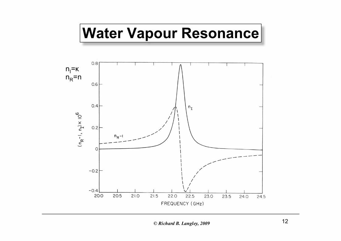
Imaginary and Real Parts of Index ofRefraction of a Gas
�
n
Resonances
© Richard B. Langley, 2009 12
Water Vapour Resonance
nI=�nR=n

© Richard B. Langley, 2009 13
Frequency, Wavelength, Wave Number, and Speed of Light
• Frequency f, angular frequency ,
wavelength �, wave number k, and the
speed of light in a medium v are related as
follows:
• In a vacuum, we have
f� =�
2�� =
�
k= v
f�0 =�
2��0 =
�
k0
= c

© Richard B. Langley, 2009 14
Dispersive Media
• In a dispersive medium, the medium’s
refractive index is a function of frequency
and hence the speed of propagation and the
wave number are functions of the EM
wave’s frequency:
v = f(�)
k = �f (�)

© Richard B. Langley, 2009 15
Dispersion Curve
• A plot of vs. k is called a dispersion curve.

© Richard B. Langley, 2009 16
Group Speed
• In a dispersive medium, waves of different
frequencies travel at different speeds. For a
modulated signal, the modulation travels at
a different speed, the group speed, than the
carrier, the phase speed:
vg =��
�k
= v+ k�v
�k

© Richard B. Langley, 2009 17
Group Refractive Index
• Associated with the group speed is the
group refractive index:
ng =c
vg
= n +��n
��
= n + f�n
�f

© Richard B. Langley, 2009 18
Solutions to the Wave Equations - 1• Various solutions to the electromagnetic
(EM) wave equations are possible including
the following:• Plane wave moving in the direction k (where
is the wave vector – don’t confuse
with the unit vector in the z-direction):
with a corresponding magnetic field solution.• Spherical waves emerging from r = 0:
k = k s
E = E0e� i(�t�k�r )
E = E0e� i(� t�k r )

© Richard B. Langley, 2009 19
Solutions to the Wave Equations - 2
• Here we have a plane wave travelling in the
z-direction:

© Richard B. Langley, 2009 20
Polarization
• E0 specifies the intensity and polarization of
the wave.
• Vector describing the electric field can be
decomposed into two orthogonal vectors,one parallel to the positive x-axis and one
parallel to the positive y-axis.
• If x- and y-components have the same
phase (or differ by an integer multiple of �),
the wave is said to be linearly polarized;
e.g., the electric field could be oriented
either horizontally or vertically.

© Richard B. Langley, 2009 21
Circular Polarization
• If the two components differ in phase, their
sum describes an ellipse about the z-axis. This
is an elliptically polarized wave.
• If the two components have the same
amplitude but are �/2 (or odd multiple of �/2)
out of phase, the ellipse becomes a circle and
the wave is said to be circularly polarized.
• If, at a fixed point, the electric (and magnetic)
field vectors rotate clockwise (counter-
clockwise) for an observer looking from the
source toward the wave propagation direction,
the polarization is right-handed (left-handed).

© Richard B. Langley, 2009 22
Right-hand Circular Polarization - 1
• If an antenna with the same polarization
sense intercepts circularly polarized waves,
the waves induce a constant signal level in
the antenna even if the antenna is rotating.
• On the other hand, if a linearly polarized
antenna intercepts a linearly polarized wave,
the electric field’s effective amplitude is
proportional to cos(�) where � is the angle
between the field polarization and antenna
directions.
• GPS EM waves are right-hand circularly
polarized.

© Richard B. Langley, 2009 23
Right-hand Circular Polarization - 2

© Richard B. Langley, 2009 24
Poynting Vector
• Specifies the magnitude and direction of
energy transport in electromagnetic fields.
At a particular point in space, it is given by
the cross (vector) product of the electric
field and the magnetic field:
• Note that s coincides with the direction of
propagation of an EM wave.
s = E� H

© Richard B. Langley, 2009 25
The Eikonal Equation - 1
• This equation is the link between physical
(wave) optics and geometric (ray) optics.
• A component of the electric field may be
written as
where A is the wave amplitude and S is
called the eikonal (from Greek for image).
• Constant values of S form a family of
wavefronts.
E(x,y,z, t) = A(x,y,z)e� i � t�k0 S(x,y,z)[ ]
© Richard B. Langley, 2009 26
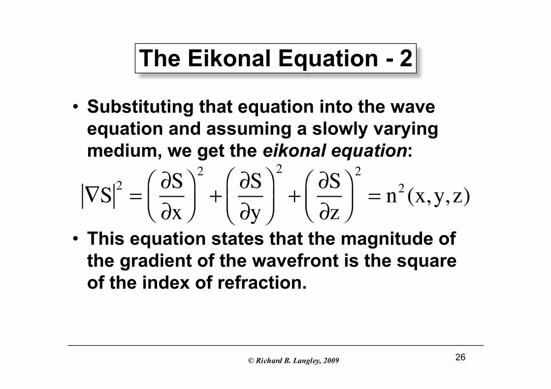
The Eikonal Equation - 2
• Substituting that equation into the wave
equation and assuming a slowly varying
medium, we get the eikonal equation:
• This equation states that the magnitude of
the gradient of the wavefront is the square
of the index of refraction.
�S2=
�S
�x���
��
2
+�S
�y
�
���
�
2
+�S
�z���
��
2
= n2 (x,y,z)

© Richard B. Langley, 2009 27
The Ray Equation - 1
• Letting r = (x,y,z) and taking �(r) to be the
perpendicular to a wavefront, we have
• Continuous curves, parallel to �(r), are
called rays.
• Taking the gradient of the eikonal equation
(with ds an increment along a ray), we get
the ray equation:
�S = n(r) s(r)
d
dsn s( ) = �n

© Richard B. Langley, 2009 28
The Ray Equation - 2
• The ray equation may be solved to find the
trajectory of a ray given n(r). For example,
let’s say that n varies only in the y direction
and the ray lies initially in the xy plane
making an angle �0 with the y axis. So, with
we have
d
dsnsin�( ) = 0
d
dsncos�( ) =
dn
dy
d
dsn �( ) = 0
s = i� + j� + k �
= isin�+ jcos�+ k �

© Richard B. Langley, 2009 29
The Ray Equation - 3
• And since
we have
• The first equation is simply Snell’s Law and
the second equation tells us the ray
remains in the xy plane.
s0 = isin�0 + jcos�0
nsin� = constant = n0 sin�0
n � = constant = 0

© Richard B. Langley, 2009 30
Snell’s Law for SphericallySymmetric Atmosphere
• Snell’s Law is slightly more complicated for
a medium in which n varies radially:
where r is the radial coordinate.
nrsin� = n0 r0 sin�0

© Richard B. Langley, 2009 31
GPS Signal Modernization
1176 MHzL5
P(Y)P(Y)
C/AC/A
P(Y)P(Y)
C/AC/AMM
Legacy Signals
Legacy and NewL2 Civil and
MilitarySignals (>2005)
Additional L5Civil
Signal(>2009)
P(Y)P(Y)
CCMM
C/AC/A
P(Y)P(Y)
CCMM
1227 MHzL2
C/AC/A
P(Y)P(Y)
MM
C/AC/A
P(Y)P(Y)
MM
1575 MHzL1

© Richard B. Langley, 2009 32
GPS Observation Equations
P(t) = �(t) + c[dtr (t) � dts (t � �)] + I(t) + T(t) + �P(t)
Pseudorange:
Carrier phase:
�(t) = � �(t)
= �(t) + c[dtr (t) � dts (t � �)] � I(t) + T(t) + �N + ��(t)
t - signal receptiontime
� - wavelengthc - speed of light - geometric range
� - signal transit time
dtr - receiver clock offset
dts - satellite clock offset
I - ionospheric delayT - tropospheric delayN - integer ambiguity�P - pseudorange noise
�� - carrier phase noise

© Richard B. Langley, 2009 33
Atmospheric Refraction
80 km
50 km
9-16 km
0 km
Ionosphere
Stratosphere
Tropopause
Troposphere
Th
erm
os
ph
ere
Me
so
sp
he
re
S’
S
� =1
vS
� dS
Refracted path
Geometric(unrefracted) path
Signal travel time:

© Richard B. Langley, 2009 34
Refractive Index of Air
• At radio frequencies, imaginary part ofrefractive index of air is negligible exceptnear the 22.235 GHz water vapour and 60GHz oxygen lines• And air is essentially a non-dispersivemedium, with n independent of frequency.• Refractive index of parcel of moist air is afunction of its temperature, partial pressureof dry constituents (nitrogen, oxygen, etc.)and partial pressure of water vapour:n = n(T, Pd, e)

© Richard B. Langley, 2009 35
Refractivity
• At sea level, values of the refractive indexof air are close to 1.0003, becoming smallerwith increasing height• A more useful quantity is refractivity, N:
with sea level values near 300
N = 106 (n �1)

© Richard B. Langley, 2009 36
Refractivity Expressions and Constants
Hydrostatic Non-hydrostatic or “Wet”
N = K1
Pd
T+ K2
e
T+ K3
e
T2
Dry Wetor
Ignoring so-called compressibility factors(they account for non-ideal behaviour ofgases with values near unity), we have:
Original formulation dueto Smith and Weintraub,1953
Revisedformulation due toDavis et al., 1985
N = K1
M
Md
P
T+ K2 � K1
M
Md
�
���
��e
T+ K3
e
T2

© Richard B. Langley, 2009 37
How We Compute N: ModernHydrostatic/Non-hydrostatic Convention
N = K1Rd�+ K2 � K1
Mw
Md
�
���
��e
T+ K3
e
T2
= K1Rd�+ K2 � K1
Rd
Rw
�
���
��e
T+ K3
e
T2
= K1Rd�+ K2
e
T+ K3
e
T2
= K1Rd
P � e
RdT+
e
RwT
�
���
��+ K2
e
T+ K3
e
T2

© Richard B. Langley, 2009 38
Definitions
P = total (barometric) pressure in millibars (mbar) =hectopascals (hPa)Pd = partial pressure of dry constituents (mbar)e = partial pressure of water vapour (mbar); can bedetermined from relative humidity and vice versaT = temperature in kelvins (K)M = molar mass of moist airMd = molar mass of dry airMw = molar mass of water vapour = density of moist airRd = gas constant for dry airRw = gas constant for water vapourK1, K2, K2', K3 = refractivity constants

© Richard B. Langley, 2009 39
Atmospheric Profiles
• Barometric pressure, temperature, andwater vapour pressure (relative humidity) varywith height above the Earth’s surface.• Barometric pressure decreases more or lessexponentially with increasing height.• Temperature and water vapour profiles aremore variable.

© Richard B. Langley, 2009 40
Standard Atmospheres

© Richard B. Langley, 2009 41
Effect of the Neutral Atmosphereon GNSS
• We turn now to consider the effect of theneutral atmosphere refraction on GNSSmeasurements.
• GNSS measurements are affected by theintegrated effects of refractivity all along thesignal raypath.

© Richard B. Langley, 2009 42
Atmospheric Refraction
80 km
50 km
9-16 km
0 km
Ionosphere
Stratosphere
Tropopause
Troposphere
Th
erm
os
ph
ere
Me
so
sp
he
re
S’
S
=1
vS
� dS
Refracted path
Geometric(unrefracted) path
Signal travel time:

© Richard B. Langley, 2009 43
Phase and Group Delay-1
�� =1
vS� dS�
1
c�S� d �S
d� = c ��
= nS� dS�
�S� d �S
= (n �1)S� dS + dS
S� � d �S
�S�
�
�
�
dP = (ng �1)S� dS + dS
S� � d �S
�S�
�
�
�
Effect ofraypathbending

© Richard B. Langley, 2009 44
Phase and Group Delay-2
• Remember: the neutral atmosphere is non-dispersive for radio waves up to a frequencyof about 20 GHz.
• So, ng = n and d� = dP.
• For a particular satellite at a particularepoch, the neutral atmosphere delay isidentical for the pseudorange and carrierphase on all the satellite’s frequencies.

© Richard B. Langley, 2009 45
Neutral Atmosphere Zenith Delay
• The zenith delay is the total delayexperienced by a signal arriving fromdirectly overhead – the zenith direction.
• Typically separated into hydrostatic andnon-hydrostatic components:
dhz = 10�6 Nhdh
r�
dnhz = 10�6 Nnhdh
r�

© Richard B. Langley, 2009 46
Tropospheric Slant Propagation Delay
T = dhzmh (�) + dnh
z mnh (�)
mapping functions
zenith delays
Zenith delay is mapped to the signal slant path atelevation angle � using a mapping function (also calledan obliquity factor):

© Richard B. Langley, 2009 47
Mapping Functions:Continued Fraction Form
m(�) =1
sin� +a
sin� +b
sin� +c
sin� +…
Setting a = 0, results in the “flat Earth” approximation(a poor model):
m(�) =1
sin�

© Richard B. Langley, 2009 48
“Two Constants” Models
m(�) =1
sin� +a
tan� + b
Continued fraction truncated after the “b term” and,in this term, sin(�) is replaced by tan(�) to ensure
that m(�) is unity at � = 90°.

© Richard B. Langley, 2009 49
m(�) =
1+a
1+b
1+ c
sin� +a
sin� +b
sin� + c
Normalized Continued Fraction Form
Used by “modern” mapping functions.
Constants determined by ray tracing (to be discussedlater) through real or modelled atmospheres.

© Richard B. Langley, 2009 50
Profile Models
Profiles (“Dry” and “Wet”)Hopfield (1969)
Yionoulis (1970)Goad & Goodman (1974)Black (1978)Black & Eisner (1984)
Saastamoinen (1973)StandardPreciseDavis et al. (1986)
Profiles (“Wet”)Chao (1972)Berman 70Berman 76

© Richard B. Langley, 2009 51
Mapping Functions
Marini (1972)Marini & Murray (1973)Chao (1972)Lanyi (1984)Davis, CfA-2.2 (1986)Ifadis (1986)Herring (1992)UNSW931 (1995)Niell (1996)Vienna Mapping Function 1, VMF1 (2006)Global Mapping Function, GMF (2006)

© Richard B. Langley, 2009 52
Combined Models (Profile + MappingFunction)
Altshuler & Kalaghan (1974)NATO (1993)Original WAAS (1995)
In general, these models do not perform as well as theothers previously mentioned,

© Richard B. Langley, 2009 53
So, How Much Delay is Imparted by theNeutral Atmosphere?
2.4 m @ 90°
24.2 m @ 5°

© Richard B. Langley, 2009 54
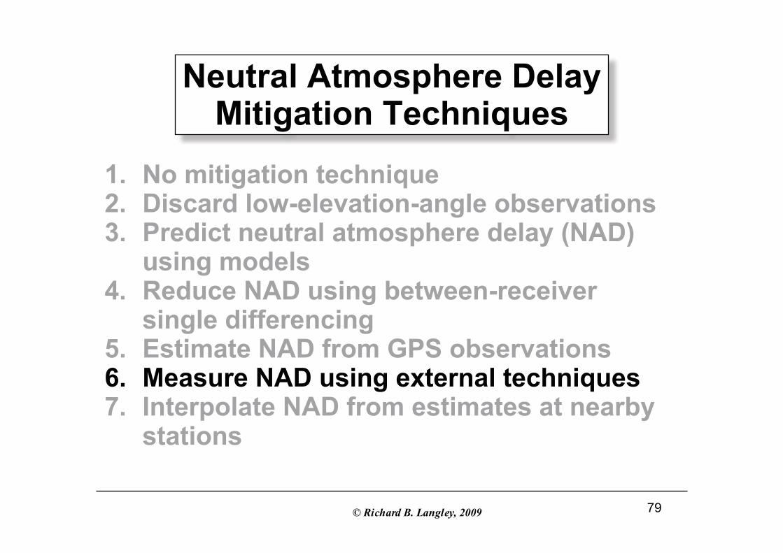
Neutral Atmosphere DelayMitigation Techniques
1. No mitigation technique2. Discard low-elevation-angle observations3. Predict neutral atmosphere delay (NAD)
using models4. Reduce NAD using between-receiver
single differencing5. Estimate NAD from GPS observations6. Measure NAD using external techniques7. Interpolate NAD from estimates at nearby
stations

© Richard B. Langley, 2009 55
Neutral Atmosphere DelayMitigation Techniques
1. No mitigation technique2. Discard low-elevation-angle observations3. Predict neutral atmosphere delay (NAD)
using models4. Reduce NAD using between-receiver
single differencing5. Estimate NAD from GPS observations6. Measure NAD using external techniques7. Interpolate NAD from estimates at nearby
stations

© Richard B. Langley, 2009 56
No Mitigation
• In standalone GNSS positioning, suffer thefull effect of the neutral atmospherepropagation delay
• Many metres of horizontal and verticalposition error.

© Richard B. Langley, 2009 57
Neutral Atmosphere DelayMitigation Techniques
1. No mitigation technique2. Discard low-elevation-angle observations3. Predict neutral atmosphere delay (NAD)
using models4. Reduce NAD using between-receiver
single differencing5. Estimate NAD from GPS observations6. Measure NAD using external techniques7. Interpolate NAD from estimates at nearby
stations

© Richard B. Langley, 2009 58
Discard Low-Elevation-AngleObservations
• Reduces the effect of neutral atmospheredelay but position error in standalonepositioning can still be at the metre level.

© Richard B. Langley, 2009 59
Neutral Atmosphere DelayMitigation Techniques
1. No mitigation technique2. Discard low-elevation-angle observations3. Predict neutral atmosphere delay (NAD)
using models4. Reduce NAD using between-receiver
single differencing5. Estimate NAD from GPS observations6. Measure NAD using external techniques7. Interpolate NAD from estimates at nearby
stations

© Richard B. Langley, 2009 60
Predict Neutral AtmosphereDelay (NAD) Using Models
• As we have seen, many profiles andmapping functions have been developed overthe years. Let’s take a look at one particularset.

© Richard B. Langley, 2009 61
UNB Neutral AtmospherePrediction Models
• A sequence of predictive, climatology-based,hybrid models• Based on Saastamoinen zenith delays, Niellmapping functions, look-up tables of sea-levelpressure, temperature, water vapour pressureor relative humidity, and lapse rate annualmeans and amplitudes, and height propagators• UNB3 widely used; basis for SBAS in-receiver model (Niell mapping functionsreplaced by simpler Black & Eisner model);application details in RTCA MinimumOperational Performance Standards document

© Richard B. Langley, 2009 62
UNB Neutral AtmospherePrediction Model Zenith Delays
dhz =
10�6 K1Rd
gm
�P0 � 1��H
T0
�
���
��
g
Rd�
dnhz =
10�6 Tm �K2 + K3( )Rd
gm �� ��Rd
�e0
T0
� 1��H
T0
�
�
��
�� g
Rd��1
Height propagators

© Richard B. Langley, 2009 63
Definitions-1
• dhz and dnh
z are the hydrostatic and non-
hydrostatic zenith delays (m)
• T0, P0, and e0 are MSL temperature (K),
barometric pressure (mbar), and water
vapour pressure (mbar) – e0 can be related to
relative humidity
• � and � are the temperature lapse rate (K m-1)
and water vapour pressure height factor
(unitless)

© Richard B. Langley, 2009 64
Definitons-2
• H is orthometric height of site (m)
• Rd is the gas constant for dry air (287.054 J
kg-1 K-1)
• gm is acceleration of gravity at atmospheric
column centroid (m s-2)
• g is standard acceleration of gravity
(9.80665 m s-2)
gm = 9.784 1� 2.66 �10�3 cos(2�)� 2.8 �10�7 H( )

© Richard B. Langley, 2009 65
Definitions-3
• Tm is the mean temperature of water vapour
(K)
• �' = � + 1 (unitless)
• K1 = 77.60 K mbar-1
• K2' = 16.6 K mbar-1
• K3 = 377600 K2 mbar-1
Tm = T0 ��H( ) 1��Rd
gm ��
�
���

© Richard B. Langley, 2009 66
UNB3
• UNB3 look-up table has 5 latitude sets of
mean (average) and annual MSL values
• Values are interpolated for latitude of station
• Day-of-year values computed from
• UNB3 is capable of predicting total zenith
delays with average uncertainties of 5 cm
under normal atmospheric conditions.
• Corresponding SBAS model error is
significantly overbounded for safety reasons
X�,doy = Avg� � Amp� �cos doy � 28)2�
365.25���
�
�
��
�

© Richard B. Langley, 2009 67
UNB3m
• In UNB3m, water vapour pressure lookupvalues are replaced with relative humidityvalues• Standard deviation of UNB3m predictionerror is similar to that of UNB3 but absolutemean error reduced by almost 75%• Package with source code in Fortran andMatLab, UNB3m_pack, has been madepublicly available (will use for lab exercise)

© Richard B. Langley, 2009 68
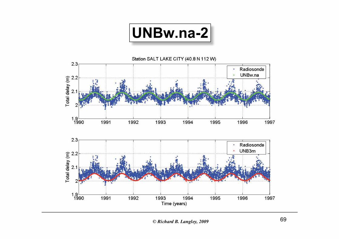
UNBw.na-1
• More reliable model for wide areaaugmentation systems users with somehomogeneity in accuracy performance overarea of interest• Based on actual surface meteorologicalvalues over many years rather than standardmodels• Look-up table is a grid of values in bothlatitiude and longitude with spacing of 5°• Initially developed for North America (0° to90° in latitude and -180° to -40° in longitude)
© Richard B. Langley, 2009 69
UNBw.na-2

© Richard B. Langley, 2009 70
UNB3w.na-3
• UNB3m is consistently better than UNB3mwith average bias reduced by about 30% andsignificant predictive performance for thesouth-western part of the U.S. (dryer, hotter,and higher)• Further details in a forthcoming paper inNavigation, the journal of The Institute ofNavigation

© Richard B. Langley, 2009 71
Neutral Atmosphere DelayMitigation Techniques
1. No mitigation technique2. Discard low-elevation-angle observations3. Predict neutral atmosphere delay (NAD)
using models4. Reduce NAD using between-receiver
single differencing5. Estimate NAD from GPS observations6. Measure NAD using external techniques7. Interpolate NAD from estimates at nearby
stations

© Richard B. Langley, 2009 72
Reduce NAD Using Between-ReceiverSingle Differencing
• This approach is used in differential GNSSpositioning.
• Delay along nearby ray paths is similar, sowhen measurements collected at a pair ofnearby receivers are differenced, the NADremaining in the differenced observations isquite small.
• Residual delay still needs to be modelled forhigh-accuracy applications.

© Richard B. Langley, 2009 73
Neutral Atmosphere DelayMitigation Techniques
1. No mitigation technique2. Discard low-elevation-angle observations3. Predict neutral atmosphere delay (NAD)
using models4. Reduce NAD using between-receiver
single differencing5. Estimate NAD from GPS observations6. Measure NAD using external techniques7. Interpolate NAD from estimates at nearby
stations

© Richard B. Langley, 2009 74
Estimate NAD From GNSS Observations
• The zenith delay can be estimated byincluding it as a parameter (deterministic orstochastic) in the data processing software(parametric least squares or Kalman filter).
• Partial derivative of an observation withrespect to the zenith delay is simply themapping function.

© Richard B. Langley, 2009 75
A Test of Options 1, 3, and 5
Three modelling options were used to process 12hours of GPS data from IGS station UNBJ inkinematic mode with GAPS (UNB’s precise pointpositioning package) and the results comparedwith the known coordinates of the station:
(a) Not accounting for the neutral atmosphere – nocorrections were applied;(b) Accounting for the neutral atmosphere using theUNB3m prediction model (seehttp://gge.unb.ca/Resources/unb3m/unb3m.html);(c) Accounting for the neutral atmosphere estimating thedelay as a random walk parameter.

© Richard B. Langley, 2009 76
Precise Point Positioning Error forDifferent Modelling Strategies

© Richard B. Langley, 2009 77
Positioning Error Statistics
(all units are metres)

© Richard B. Langley, 2009 78
Gradient Models
• Many neutral atmosphere delay modelsassume azimuthal symmetry; i.e., theatmosphere is assumed to be the same allaround a site.• Clearly this doesn’t match reality particularlyduring the passage of weather fronts.• Models have been enhanced by includinggradient terms that can be estimated from theGNSS data.
© Richard B. Langley, 2009 79
Neutral Atmosphere DelayMitigation Techniques
1. No mitigation technique2. Discard low-elevation-angle observations3. Predict neutral atmosphere delay (NAD)
using models4. Reduce NAD using between-receiver
single differencing5. Estimate NAD from GPS observations6. Measure NAD using external techniques7. Interpolate NAD from estimates at nearby
stations

© Richard B. Langley, 2009 80
Ray Tracing Through RadiosondeProfiles or Numerical Weather Models
• Radiosondes (also known asweather balloons) are launchedfrom many locations around theworld twice a day.
• Pressure, temperature, andrelative humidity measurementsare send by radio to the ground.
• The profiles can be used todetermine refractivity at pointsalong a path entering or leaving theatmosphere at a particularelevation angle.
• The same procedure can be usedwith numerical weather models.

© Richard B. Langley, 2009 81
Water Vapour Radiometer
• Measures brightness temperature at two or
more frequencies near and adjacent to the
water vapour line
• Radiometrics WVR-1100 uses 23.8 and 31.4
GHz
• Measurements converted
to wet tropospheric delay
along direction of
measurement using
calibration constants
• Accuracies typically better than 1 centimetre

© Richard B. Langley, 2009 82
Neutral Atmosphere DelayMitigation Techniques
1. No mitigation technique2. Discard low-elevation-angle observations3. Predict neutral atmosphere delay (NAD)
using models4. Reduce NAD using between-receiver
single differencing5. Estimate NAD from GPS observations6. Measure NAD using external techniques7. Interpolate NAD from estimates at nearby
stations

© Richard B. Langley, 2009 83
Interpolate NAD From Estimates atNearby Stations
• This approach is used in real-timedifferential GNSS, such as DGPS and real-time kinematic (RTK) positioning.
• In pseudorange-based DGPS, thetransmitted correction includes the effect ofNAD as experienced at the reference station.
• In network RTK, an interpolated zenith NADcan be sent to the user.

© Richard B. Langley, 2009 84
Using GNSS to Measure AtmosphericMoisture Content
• Precipitable water (vapour), the total atmosphericwater vapour in a vertical column of unit cross-sectional area in terms of the height to it wouldstand if completely condensed and collected in avessel of the same unit cross section (PW), isproportional to the zenith wet delay (ZWD)• ZWD is estimated from GNSS measurementsafter removing hydrostatic delay computed fromaccurate surface pressure measurements• 10 mm PW corresponds to about 65 mm of ZWD• 1 mbar error in surface pressure could result in0.4 mm error in precipitable water

© Richard B. Langley, 2009 85
Monitoring Networks
Several GNSS monitoring networks have beenestablished in different parts of the world fordetermining precipitable water; e.g., theUniversity Corporation for AtmosphericResearch (UCAR) SuomiNet, the U.S. NationalOceanic and Atmospheric Administration’sGlobal Systems Divison Ground-Based GPSMeteorology (GPS-MET), etc.

© Richard B. Langley, 2009 86
SuomiNet
About 60 sites inthe U.S.A.,Canada, and theCaribbean
Sites use Trimbleequipment andmost haveauxiliary metsensors
Animation:http://www.unidata.ucar.edu/data/suominet/loop/suomi_ani.html

© Richard B. Langley, 2009 87
GPS-MET
Over 500 sites in North America

© Richard B. Langley, 2009 88
Rapid Update Cycle (RUC) WeatherPrediction
RUC 13 =13 kmresolutionmodel,updatedhourly withpredictionsout to 12hours +

© Richard B. Langley, 2009 89
Hurricane Forecasting
animation:http://gpsmet.fsl.noaa.gov/jsp/katrina2.jsp

© Richard B. Langley, 2009 90
German GPS Met Network

© Richard B. Langley, 2009 91
Estimated Water Vapour Field
Integrated water vapour (IWV)= PWV • density of H2O
IWV(kg/m2)
15 August 200012:00 UT

© Richard B. Langley, 2009 92
Atmosphere Profiling Using GNSSReceivers Onboard LEO Satellites
• Dual-frequency GNSS receiver on low Earthorbiting (LEO) satellite• Signal raypaths of rising and setting GNSSsatellites as viewed from the LEO are bent bythe atmosphere• The bending angle can be measured andrelated to the refractive index at the height ofthe ray• Refractive index can be interpreted to giveprofiles of temperature

© Richard B. Langley, 2009 93
Spaceborne GPS Limb Sounding

© Richard B. Langley, 2009 94
LEO Atmospheric Profiling Satellites
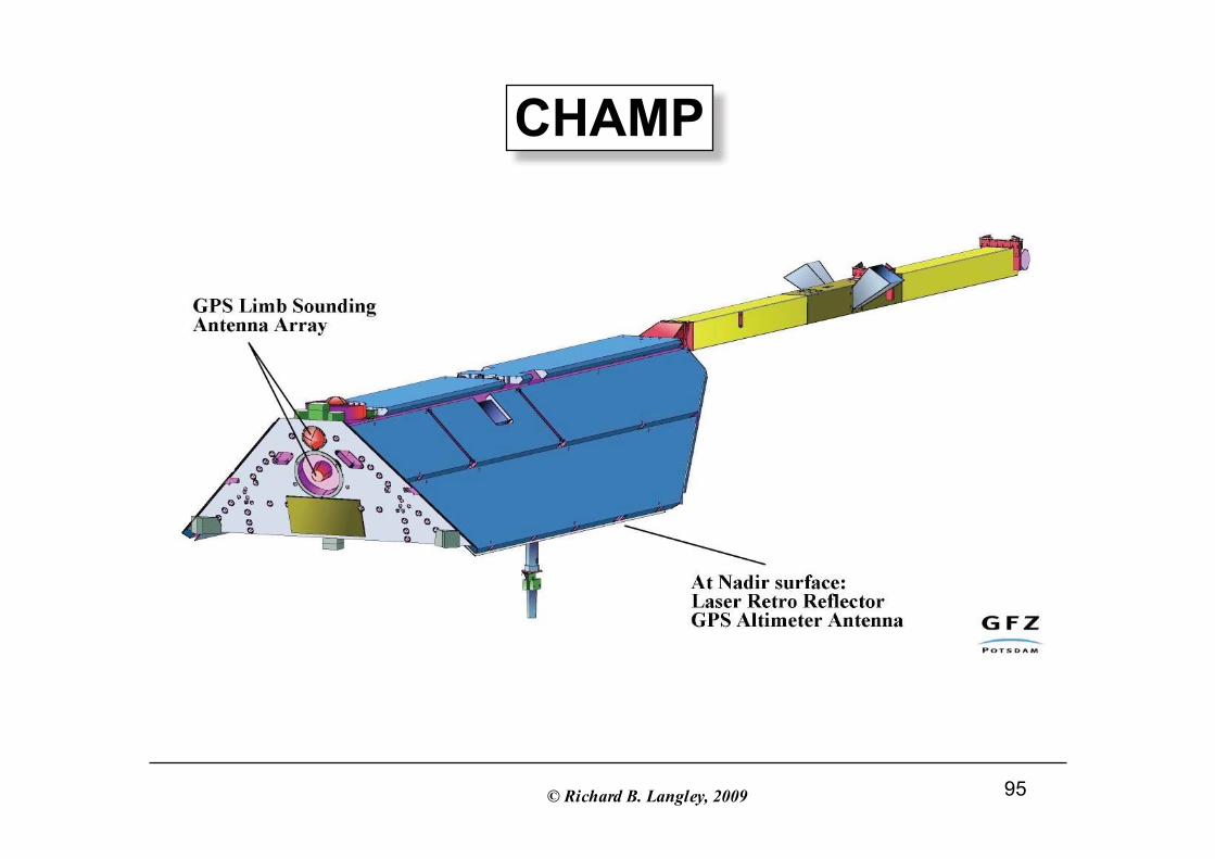
A number of satellites with this capability havebeen launched:GPS-Met, U.S.A. (1995)CHAMP, Germany (2000)SAC-C, Argentina (2000)COSMIC (6 satellites), Taiwan and U.S.A. (2006)METOP-A, Europe (2006)…
© Richard B. Langley, 2009 95
CHAMP

© Richard B. Langley, 2009 96
CHAMP Profiling
CHAMP datataken over theSouth Atlantic on 11 February 2001

© Richard B. Langley, 2009 97
What Have We Learned?
• The physics of the propagation of radiosignals through the neutral atmosphere.
• How the neutral atmosphere affects GNSSmeasurements.
• How to mitigate the effects of the neutralatmosphere in GNSS positioning.
• How GNSS signals can be used to remotelysense atmospheric properties.

© Richard B. Langley, 2009 98
Practical Lab
In the lab, you will download UNB3m_pack, aneutral atmosphere delay package forradiometric space techniques, and work withit in the MatLab programming environmentto see how the prediction of delays varieswith location, station height, and day of year.

© Richard B. Langley, 2009 99
Thanks, Grazie, Ahsante