2016 annual conference & exposition sun05 – … · 2016 annual conference & exposition ....
TRANSCRIPT

2016 Annual Conference & Exposition
SUN05 – Designing a Risk-based Pipeline R&R Planning Program Using a
Combination of Inspection and Analytical Approaches
June 19, 2016 Chicago, Illinois

Workshop Agenda
9:00 Welcome Annie Vanrenterghem Raven, infraPLAN 9:05 Introduction Kevin Campanella, Burgess & Niple 9:15 Introduction Questionnaire Kevin Campanella, Burgess & Niple 9:20 AM Framework and Data Kurt Vause, streamlineAM, LLC 9:40 Data Clean-up Exercises Annie Vanrenterghem Raven, infraPLAN 10:30 Break 10:40 Analytical Approach: From Basic to Advanced Approach Non-Inspected and Inspected Pipes Annie Vanrenterghem Raven, infraPLAN Celine Hyer, ARCADIS 11:40 Case Study: Columbus – From Basic to Advanced Approach Non-Inspected Pipes Kevin Campanella, Burgess & Niple noon Lunch 1:00 Q/A About Columbus Kevin Campanella, Burgess & Niple 1:10 Case Study: Dallas – From Basic to Advanced Approach Inspected Pipes Annie Vanrenterghem Raven, infraPLAN Celine Hyer, ARCADIS

1:40 Group Discussion: Where do you stand? Where do you want to go? Celine Hyer, ARCADIS Kurt Vause, streamlineAM, LLC 2:40 Break 2:50 Synthesis of Previous Discussion Kevin Campanella, Burgess & Niple 3:00 Mixing Analytical Approach and Inspection Program Annie Vanrenterghem Raven, infraPLAN 3:25 Case Study: AWWU –Mixing Analytical Approach with Inspection Program Kurt Vause, streamlineAM, LLC 3:55 Wrap-up Annie Vanrenterghem Raven, infraPLAN

Presenter Information
Annie Vanrenterghem Raven, infraPLAN [email protected]
Bio: For the last 20 years, Annie’s research and consulting work have focused on water and waste water infrastructure, addressing the optimal planning of short and long-term rehabilitation projects. She is now the Managing Director of infraPLAN, a firm she created in 2008 that develops analytical models translated in functional software, and provides consulting and training. The goal is to help utilities create comprehensive and Advanced Analytical Asset Management programs, and, ultimately, identify and justify their long-term investments, and short-term projects selection. Annie is a member of the AWWA Asset Management Committee’s Advisory Committee. She holds a Ph.D. in Civil Engineering, Polytechnic Institute of New York University, New York, NY.
Celine Hyer, ARCADIS [email protected]
Bio: Celine is the National Conveyance Market Sector Leader within ARCADIS and is located in their Tampa Florida office. She has a B.S. in Chemical Engineering and an M.S. in Engineering Management from Florida Institute of Technology. Celine has 25 years of experience in Engineering with 15 years that are directly related to asset management program implementations including advanced renewal and replacement planning for pipelines as well as treatment and pumping facilities. Celine currently serves as the Secretary of the AWWA Asset Management Committee and as the Chairwoman of the Industry Advisory Board for the Sustainable Water Infrastructure Center at Virginia Tech.
Kurt Vause, streamlineAM [email protected]
Bio: From 1998 - 2015, Kurt was Engineering Division Director of Anchorage Water Wastewater Utility. He was responsible for AWWU’s capital construction program, its Grants & Loans section, and the utility’s Strategic Asset Services and Planning sections. In 2016, he became Special Projects Director providing planning, integration, and execution of strategic utility initiatives. Kurt currently serves on American Water Works Association’s Water Utility Council, presently serving as the Regulatory Subcommittee chair and is Incoming Chair of the Council. In addition, he is a member and Vice-Chair of AWWA’s Asset Management Committee. He also served on the 2012 International Water Association - Water Supply Association of Australia Asset Management Best Practices Benchmarking Project Steering

Committee. He is co-founder of StreamlineAM, LLC, an Alaskan-based consulting service dedicated to utility management, asset management, and engineering for the water sector.
Kevin Campanella, BURGESS & NIPLE [email protected]
Bio: Kevin has been in the asset management services field for 14 years. In 2002, he moved to New Zealand to work with Meritec, joining some of the authors of the original International Infrastructure Management Manual. From 2003 to 2008, he worked for Brown and Caldwell, developing asset management solutions with the Columbus Division of Sewerage and Drainage to address their CMOM consent order. For seven years beginning in 2008, he led the comprehensive asset management program at the Columbus Department of Public Utilities as an Assistant Director. Kevin is a member of the AWWA Asset Management Committee’s Advisory Committee, is chair of the “Progress in Asset Management Survey” subcommittee, and is Vice Chair of the Ohio AWWA Asset Management Committee.

Kevin Campanella
Celine Hyer
Annie Vanrenterghem Raven
Kurt Vause
1
Designing a Risk-based Pipeline R&R Planning
Program using a Combination of Inspection and
Analytical Approaches
Our Speakers
2
Annie Vanrenterghem RaveninfraPLAN
Celine HyerARCADIS
Kurt VausestreamlineAM
Kevin CampanellaBURGESS & NIPLE
2
09:00-9:05Welcome
Annie
9:05-9:15
Introduction
Kevin
9:15-9:20
Introduction Questionnaire
Kevin
9:20-9:40
AM Framework and Data
Kurt
9:40-10:30
Data clean-up Exercises
Annie et al
10:30-10:40
BREAK
10:40-11:40
Analytical Approach – From Basic to Advanced Approach
non-inspected and Inspected Pipes
Annie and Celine
11:40-12:00
Case Study: Columbus – From Basic to Advanced Approach
non-inspected Pipes
Kevin
1:00-1:10
Q/A about Columbus
Kevin
1:10-1:40
Case Study: Dallas – From Basic to Advanced Approach
Inspected Pipes
Celine and Annie
1:40-2:40
Group Discussion
Where do you stand? Where do you want to go?
Celine, Kevin, Kurt
2:40-2:50
BREAK
2:50-3:00
Synthesis of Previous Discussion
Kevin
3:00-3:25
Mixing Analytical Approaches and Inspection Program
Annie
3:25-3:55
Case Study: AWWU – From Basic to Advanced Approach
Mixing Analytical Approach with Inspection Program
Kurt
3:55-4:00 Wrap-up
Annie
3
12:00-1:00LUNCH
Workshop Agenda
3

44
5
6

7
8
9

10
11
What you will learn?
12
You will learn:
1. about approaches, from basic to advanced, to manage in a cost efficientway the planning of Inspection, Rehabilitation & Replacement (R&R) of water pipelines using utility-specific data whether they are inspected or not
2. about tradeoffs inherent to these approaches in terms of benefits(increasing accuracy of when and what to inspect, rehabilitate or replace; and avoiding risk of asset failure) and costs (data requirements and level of effort)
3. to identify, mine, clean-up, format and analyze the data needed to successfully use these advanced approaches
4. where your organization stands and where it wants to go
5. from experts who have been applying these approaches and, as a result, have specific case studies and lessons to share

Why is this an important topic?
• Linear buried water assets = 2/3 of the value of water infrastructure
• Substantial percentage is approaching end of Effective Useful Life (EUL)
• Discrepancy between projected cost of next CIP and R&R needs, and analytical justification or reliance on analytics, to optimize program
• $ will need to be -and can- be stretched using powerful and convincingammunitions!
• Physical Condition Assessment (PCA) still $$ and proportional to length reliance on analytics $ is not proportional to length
13
Why should you prefer advanced approaches?
• More accurate projections (but, not always longer EULs)
• Optimization of resources and savings (using risk-based approach)
• Possibility to explore many different long term planning options
• More granularity in results - larger choice of projects to prioritize
• More defensible, justifiable, credible budget projections
14
0
500
1,000
1,500
2,000
2,500
3,000
3,500
4,000
4,500
2014 2050 2100
Co
st $
M
Year
Industry-Assumed EULs
Cumulative Cost up to 2050 and 2100 based on Industry-Assumed EULs
15
System North East US with medium average break rate - 1,200 mi
$1.8B
$4B

0
500
1,000
1,500
2,000
2,500
3,000
3,500
4,000
4,500
2014 2050 2100
Co
st $
M
YearIndustry-Assumed EULs Utility- and Risk-Specific EULs
65% Reduction ($1.2B)
50% Reduction ($2B)
Results with Advanced ApproachUtility- and Risk-Specific EULs
16
A few words of wisdom about data • Data quality matters with any approach or any software, from basic to advanced.
• Even a simple break rate will be wrong if definition of breaks, number of breaks, length of pipes, and number of years are wrong.
• Precision is not so much the goal (but precise results are of course preferred!). We do not want wrong estimates. Which is what using generic and assumed data, andsimplistic approaches can lead to.
• It does not take more time or effort to collect the right (break and pipe) data in the right format.
• It does take time to clean-up old data (never collected for planning) but this is tobe done once for all.
• Once data is Okay (old one cleaned-up; new one properly restructured andformatted) why not use appropriate and advanced approaches that provide more reliable and defensible answers; that make requests more credible and easier tojustify?
17
09:00-9:05Welcome
Annie
9:05-9:15
Introduction
Kevin
9:15-9:20
Introduction Questionnaire
Kevin
9:20-9:40
AM Framework and Data
Kurt
9:40-10:30
Data clean-up Exercises
Annie et al
10:30-10:40
BREAK
10:40-11:40
Analytical Approach – From Basic to Advanced –
Non-inspected and Inspected Pipes
Annie and Celine
11:40-12:00
Case Study: Columbus – From Basic to Advanced Approach
Non-inspected Pipes
Kevin
1:00-1:10
Q/A about Columbus
Kevin
1:10-1:40
Case Study: Dallas – From Basic to Advanced Approach
Inspected Pipes
Celine and Annie
1:40-2:40
Group Discussion
Where do you stand? Celine
Where do you want to go? Kurt
2:40-2:50
BREAK
2:50-3:00
Synthesis of Previous Discussion
Kevin
3:00-3:25
Mixing Analytical Approach and Inspection Program
Annie
3:25-3:55
Case Study: AWWU – From Basic to Advanced Approach
Mixing Analytical Approach with Inspection Program
Kurt
3:55-4:00 Wrap-up
Annie
18
12:00-1:00LUNCH
Workshop Agenda

Questionnaire
• Handout 1
• Presentation of questionnaire that will be used for Celine, Kevin and Kurt’ session in the afternoonWhere does your organization stand?
Where does your organization want to go?
• While attending the upcoming presentations, reflect on where your organization stands and where it would like to go; the data, tools, resources currently at your disposal (or not).
19
09:00-9:05Welcome
Annie
9:05-9:15
Introduction
Kevin
9:15-9:20
Introduction Questionnaire
Kevin
9:20-9:40
AM Framework and Data
Kurt
9:40-10:30
Data clean-up Exercises
Annie et al
10:30-10:40
BREAK
10:40-11:40
Analytical Approach – From Basic to Advanced –
Non-inspected and Inspected Pipes
Annie and Celine
11:40-12:00
Case Study: Columbus – From Basic to Advanced Approach
Non-inspected Pipes
Kevin
1:00-1:10
Q/A about Columbus
Kevin
1:10-1:40
Case Study: Dallas – From Basic to Advanced Approach
Inspected Pipes
Celine and Annie
1:40-2:40
Group Discussion
Where do you stand? Celine
Where do you want to go? Kurt
2:40-2:50
BREAK
2:50-3:00
Synthesis of Previous Discussion
Kevin
3:00-3:25
Mixing Analytical Approach and Inspection Program
Annie
3:25-3:55
Case Study: AWWU – From Basic to Advanced Approach
Mixing Analytical Approach with Inspection Program
Kurt
3:55-4:00 Wrap-up
Annie
20
12:00-1:00LUNCH
Workshop Agenda
FrameworkFrom Basic to Advanced
21

Assumed
EULs
InventoryLong-Term
Plan
Basic Framework
22
Cost
R&R
COF
Weighted
Score
LOF
Weighted
Score
Risk Score and
Short-Term
Prioritization Plan
Answer Q1
How much money
is needed until
2050?
Answer Q2
What projects
should be
addressed first?
Advanced Framework
• Non-inspected pipes failure data
• Inspected pipes inspection records
23
Non-Inspected Pipes
24
Break Cons.
of
Failure
GIS Pipes
Failure
Forecasting
CMMS Aging
Function
EULs
Long –Term
R&R Plan
Criticality and
Risk Score
Likelihood
of
Failure
Asset
Management
Plan
Clean-up
Statistics
GIS Breaks
Short -Term
Prioritization
Plan
Utility Data
Software-
algorithm
Output - Input
Where is
info about
pipes
attributes?
Where is
info about
breaks?
How is future
behavior
predicted?
What are the
output results
from a failure
forecasting
model?
Answer Q1
How much money
is needed until
2050?
Answer Q2
What projects
should be
addressed first?
Inventory
Hydraulic
CriticalityCost
R&R
Other
Criteria

Inspected Pipes
25
GIS Pipes
Physical
Condition
Forecasting
CMMS
Likelihood
of
Failure
Clean-up
Statistics
Inspection records
Utility Data
Software-
algorithm
Output - Input
Where is
info about
pipes
attributes?
Where is info
about
inspection?
How is future
behavior
predicted?
Inspected Pipes
26
Cost
Failure Cons.
of
Failure
GIS Pipes
Physical
Condition
Forecasting
CMMS Aging
Function
EULs
Long –Term R&R
and Inspection
Plan
Criticality and
Risk Score
Likelihood
of
Failure
Asset
Management
Plan
Clean-up
Statistics
Inspection records
Short -Term
Prioritization
Plan
Utility Data
Software-
algorithm
Output - Input
Where is
info about
pipes
attributes?
Where is
info about
inspection
?
How is future
behavior
predicted?
Inventory
Hydraulic
CriticalityCost
R&R & Insp.
Other
Criteria
Key Elements of the AM Plan
27
Cost
Break
Cons.
of
Failure
GIS Pipes
Failure /PCA
Forecasting
CMMS Aging
Function
EULs
Long -Term
Plan
Criticality and
Risk Score
Likelihood
of
Failure
Asset
Management
Plan
clean-up
Statistics
GIS Breaks
Short -Term
Prioritization
Plan
Inventory
Hydraulic
CriticalityR&R
LTP STP
Aging
Curve
EUL
COF
LOF
Other
Criteria

Data
28
Pipe Data
• System level
Inventory from purchasing records
(pre GIS).
• Pipe level
Pipe Data Base (DB) or GIS.
Pipe-level statistics.
• Active (ACT) and Abandoned
(ABN) pipes
Better failure statistics
29
FEATID DOI DISTRICT DIAM MAT LENGTH LIFE STATUS
DOA SOIL ROAD
17608 1/1/1934 Ridgefield 2 SCI 0.0033 ABN 12/20/2003 1 2
17609 1/1/1934 Ridgefield 2 SCI 0.0033 ABN 12/20/2003 2 3
17610 1/1/1936 Ridgefield 2 SCI 0.0544 ABN 12/20/2003 3 1
10946 5/31/1949 Bridgeport 8 SCI 0.0967 ACT 2 2
10947 1/10/1961 Bridgeport 8 SCI 0.0681 ACT 2 3
10948 6/9/1905 Bridgeport 24 PCI 0.1992 ACT 1 3
10949 2/18/1909 Bridgeport 4 PCI 0.0598 ACT 2 1
10950 3/10/1923 Bridgeport 12 PCI 0.0143 ACT 2 1
10952 11/27/1963 Stratford 8 SCI 0.058 ACT 3 1
Non-Inspected PipesBreak Data
• Break DataLocation, Type, Date Of Break (DOB)
• Not geocoded/pre GIS– Break reports/CMMS– Address; no pipe ID; not connected to the pipe data
generic failure statistics aging function and Effective Useful Life (EUL) have to beassumed
• Geocoded/GIS– Same + Pipe ID
Pipe linked to YOI and Age Time-related statistics aging function and EUL computed
• Active (ACT) and Abandoned (ABN) better failure statistics, forecast and aging functions if ABN data is available.
30
BREAK DATA
PRE GISLOCATION MAT DIAM DATE OF BREAK
10 Main street CI 12 7-Jun-15
POST GIS101 CI 12 7-Jun-15
PIPE DATAPIPE ID MAT DIAM YOI LENGTH
101 CI 12 1900 200

Importance of Pipe and Break Information about Abandonment
Imagine worse pipes have been abandoned between 85 and 95 but abandonment data is not available.
we will predict behavior of all mains that are now between 65-75, when they are 85-95, based on best pipes; not whole array
optimistic EULs
under-estimated R&R predictions
Example:• pipes installed between 1920 and 1950 are now between 65 and 95 yrs old.
• pipes degrade same way (same cohort) but for each YOI there are better or worse pipes.
• we have 10 years of breaks 2005-2015.
• when pipes reach high break rate (between 85 and 95) they are replaced. Between 2005-2015 this applied to pipes installed between 1920 and 1930.
• by age of 85-95 best pipes are left.
• EUL 105 instead of 95
31
Break Rate based on Year of Installation (ACT Mains Only)
32
0
5
10
15
20
25
30
35
40
192
0
192
1
192
2
192
3
192
4
192
5
192
6
192
7
192
8
192
9
193
0
193
1
193
2
193
3
193
4
193
5
193
6
193
7
193
8
193
9
194
0
194
1
194
2
194
3
194
4
194
5
194
6
194
7
194
8
194
9
195
0
Bre
ak R
ate
(Nb
Bre
aks/
mi/
yr)
Year of Installation
Break Rate based on Year of Installation
Break Rate Based on Age at Year of Break
0
5
10
15
20
25
30
35
40
65
66
67
68
69
70
71
72
73
74
75
76
77
78
79
80
81
82
83
84
85
86
87
88
89
90
91
92
93
94
95
96
97
98
99
100
101
102
103
104
105
Bre
ak R
ate
(Nb
Bre
aks/
10
0 m
i/yr
)
Age at Year of Break
Break Rate based on Age at Year Of Break
Break Rate 1 - no info on RPLT Break Rate 2 - info on RPLT
Expon. (Break Rate 1 - no info on RPLT) Expon. (Break Rate 2 - info on RPLT)
95 105
20
Inspected Pipes Inspection Data
• Inspection Data
– Location, Type (technology, contractor),
Date of Inspection
• Data Base (address) or GIS (ID)
– Same issue as with non-inspected pipes
33

Major Differences between Break and Inspection Data
• Need break history for all pipes and all years during window of observation of breaks
• Not the case for inspection data: can be any year and any pipe
34
0
50
100
150
200
250
300
0
0.05
0.1
0.15
0.2
0.25
19
84
19
86
19
88
19
90
19
92
19
94
19
96
19
98
20
00
20
02
20
04
20
06
20
08
20
10
20
12
20
14
20
16
Len
gth
(m
i)
Bre
ak R
ate
(Nb
Bre
aks/
mi/
yr.)
YOB
Net Cumulative Length and Break Rate based on YOB
Break Rate Length Linear (Break Rate)
Zip Code Breaks 1990-2015 Length10014 200 10010015 250 10010016 300 10010017 150 10010018 220 10010019 400 10010020 2 100
PipeID Inspection Date Inspection Score101 1990 1101 2005 2101 2010 3102 2015 3103
Breaks missing in
certain areas
and at certain years
Pipes not all inspected and not every year
Main Issues with Pipe, Break and Inspection Data
• Issues
– Definition
– Incomplete
– Missing
– Assumed
– Incorrect
– Incoherent
– Questionable
– Limited
– Consistent
• How to identify and clean-up issues? What does it take?
– Manually or diagnostic /clean-up algorithms
– Assumptions/statistics
– clean-up may require going back to some historical records35
OBJECTID PlacementI PlacementS
Placement
D
Placement
M SourceScal UpdateId
UpdateDat
e
UpdateMet
h UpdateSour FeatureId DateInsta l Dis trict
19 WLS FLDSKETCH 10/17/2006 DIGITIZED NTS sdemezzo 7/20/2011 ORIGINAL ORIGINAL 292143 2109000
20 WLS FLDSKETCH 10/17/2006 DIGITIZED NTS sdemezzo 7/20/2011 ORIGINAL ORIGINAL 292149 2109000
24 WLS FLDSKETCH 10/17/2006 DIGITIZED NTS sdemezzo 7/20/2011 ORIGINAL ORIGINAL 292171 2109000
29 WLS FLDSKETCH 10/18/2006 DIGITIZED NTS ORIGINAL ORIGINAL 292207 1/1/2000 2109000
30 WLS FLDSKETCH 10/18/2006 DIGITIZED NTS ORIGINAL ORIGINAL 292209 1/1/2000 2109000
31 WLS FLDSKETCH 10/18/2006 DIGITIZED NTS ORIGINAL ORIGINAL 292210 1/1/2000 2109000
32 WLS FLDSKETCH 10/18/2006 DIGITIZED NTS sdemezzo 7/20/2011 ORIGINAL ORIGINAL 292212 2109000
33 WLS FLDSKETCH 10/20/2006 DIGITIZED NTS ORIGINAL ORIGINAL 292303 1/1/2000 2109000
34 WLS FLDSKETCH 10/20/2006 DIGITIZED NTS ORIGINAL ORIGINAL 292304 1/1/2000 2109000
35 WLS FLDSKETCH 10/19/2006 DIGITIZED NTS ORIGINAL ORIGINAL 292249 1/1/2000 2109000
44 WLS FLDSKETCH 10/20/2006 DIGITIZED NTS sdemezzo 7/20/2011 ORIGINAL ORIGINAL 292311 2109000
45 WLS FLDSKETCH 10/31/2006 DIGITIZED NTS ORIGINAL ORIGINAL 292763 1/1/2000 2109000
46 WLS FLDSKETCH 10/31/2006 DIGITIZED NTS sdemezzo 7/20/2011 ORIGINAL ORIGINAL 292764 2109000
47 WLS FLDSKETCH 10/31/2006 DIGITIZED NTS ORIGINAL ORIGINAL 292768 9/30/1997 2109000
48 WLS FLDSKETCH 10/31/2006 DIGITIZED NTS ORIGINAL ORIGINAL 292766 1/1/2000 2109000
49 WLS FLDSKETCH 10/31/2006 DIGITIZED NTS ORIGINAL ORIGINAL 292769 1/1/2000 2109000
50 WLS FLDSKETCH 10/31/2006 DIGITIZED NTS sdemezzo 7/20/2011 ORIGINAL ORIGINAL 292790 2109000
51 WLS FLDSKETCH 10/31/2006 DIGITIZED NTS ORIGINAL ORIGINAL 292791 1/1/2000 2109000
52 WLS FLDSKETCH 10/31/2006 DIGITIZED NTS ORIGINAL ORIGINAL 292792 1/1/2000 2109000
53 WLS FLDSKETCH 10/31/2006 DIGITIZED NTS ORIGINAL ORIGINAL 292808 1/1/2000 2109000
54 WLS FLDSKETCH 10/31/2006 DIGITIZED NTS ORIGINAL ORIGINAL 292805 1/1/2000 2109000
55 WLS FLDSKETCH 10/31/2006 DIGITIZED NTS ORIGINAL ORIGINAL 292804 1/1/2000 2109000
56 WLS FLDSKETCH 10/31/2006 DIGITIZED NTS ORIGINAL ORIGINAL 292807 1/1/2000 2109000
57 NA LEGACY 10/21/2004 MIGRATED 500 WOOLPERT 7/7/2005 DIGITIZED CONVERSION 126231 1/1/2000 2109000
58 NA LEGACY 10/21/2004 MIGRATED 500 sdemezzo 7/20/2011 DIGITIZED CONVERSION 126234 2109000
59 WOOLPERT CONVERSION 7/7/2005 DIGITIZED UNK sdemezzo 7/20/2011 ORIGINAL ORIGINAL 306616 2109000
Data QualityPast and Future
• 2 levels of data:
– Past
– Future
• 2 Goals for data diagnostic :
– Identify issues and clean-up past data (eventually)
– Restructure future data (and never have to clean-up data again!)
36

Other Data
• Operations/hydraulic– hydraulic capacity
– fire flow
– pressure
– service points
– consumption
– water quality
– leaks
• Service – customers criticality
– complaints (shortage, water quality, frequency of construction projects)
– planned work for sewers or pavement
37
• Cost – repair (from basic to very advanced
if indirect and social costs included)
– rehabilitation
– replacement
• Environmental/location – soil
– traffic
– population density/construction
– sensitive targets (rail track, subway entrance, tunnel)
09:00-9:05Welcome
Annie
9:05-9:15
Introduction
Kevin
9:15-9:20
Introduction Questionnaire
Kevin
9:20-9:40
AM Framework and Data
Kurt
9:40-10:30
Data clean-up Exercises
Annie et al
10:30-10:40
BREAK
10:40-11:40
Analytical Approach – From Basic to Advanced –
Non-inspected and Inspected Pipes
Annie and Celine
11:40-12:00
Case Study: Columbus – From Basic to Advanced Approach
Non-inspected Pipes
Kevin
1:00-1:10
Q/A about Columbus
Kevin
1:10-1:40
Case Study: Dallas – From Basic to Advanced Approach
Inspected Pipes
Celine and Annie
1:40-2:40
Group Discussion
Where do you stand? Celine
Where do you want to go? Kurt
2:40-2:50
BREAK
2:50-3:00
Synthesis of Previous Discussion
Kevin
3:00-3:25
Mixing Analytical Approach and Inspection Program
Annie
3:25-3:55
Case Study: AWWU – From Basic to Advanced Approach
Mixing Analytical Approach with Inspection Program
Kurt
3:55-4:00 Wrap-up
Annie
38
12:00-1:00LUNCH
Workshop Agenda
Real Life Data Data Clean-up Exercise
• Non-inspected– Pipe and break data
– Pipe and break data quality diagnostic
– Identify issues in sample datasets – handout 2
• Inspected– Pipe and inspection data
– Pipe and inspection data quality diagnostic
– Identify issues in sample datasets – handout 3
39

Non-inspected Pipe and Break Data
• 3,194 mi system in North East (10% rejected)
• 2,105 breaks ranging between 2007 and 2013 (13% rejected)
• ACT and ABN pipe data
40
Pipes Issues - Summary
41
SELECTION OR QUALITY ISSUESAbandoned before installed. DIAM < 4. Duplicate Feature ID. Early abandonment (< 3). L < 0.0002. No DIAM. No DOI. No MAT. Suspicious DOI or MAT.
No Issue 2,870.93 90%Issues 323.39 10%Total 3,194.32 1
Pipe Issues-
Breakdown
42
Issues Length (mi)Abandoned before installed. 0.14
DIAM < 4. 24.78
DIAM < 4. L < 0.0002. 0
DIAM < 4. Suspicious DOI or MAT. 0.01
Duplicate Feature ID. 4.89
Duplicate Feature ID. DIAM < 4. 0.65
Duplicate Feature ID. Early abandonment (< 3). 0.05
Early abandonment (< 3). 1.63
L < 0.0002. 0.01
No DIAM. 6.19
No DIAM. L < 0.0002. 0
No DOI. 100.34
No DOI. DIAM < 4. 16.24
No DOI. Duplicate Feature ID. 0.46
No DOI. Duplicate Feature ID. DIAM < 4. 0.46
No DOI. L < 0.0002. 0
No DOI. No DIAM. 0.22
No MAT. 1.42
No MAT. DIAM < 4. 0.05
No MAT. No DIAM. 0.06
No MAT. No DOI. 134.75
No MAT. No DOI. DIAM < 4. 12.53
No MAT. No DOI. Duplicate Feature ID. 0.12
No MAT. No DOI. Duplicate Feature ID. No DIAM. 0.25
No MAT. No DOI. L < 0.0002. 0
No MAT. No DOI. No DIAM. 7.57
Suspicious DOI or MAT. 10.54
No Issue 2,870.93
Total 3,194.32
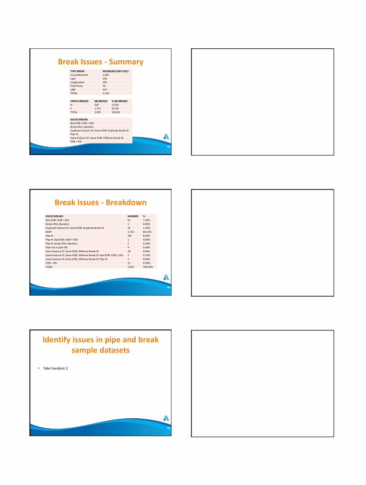
Break Issues - Summary
43
TYPE BREAK NB BREAKS 2007-2013
Circumferential 1,067
Leak 236
Longitudinal 395
Third Party 70
UNK 337
TOTAL 2,105
STATUS BREAKS NB BREAKS % NB BREAKS
N 264 13.0%
Y 1,771 87.0%
TOTAL 2,035 100.0%
ISSUES BREAKS
Bad DOB: DOB < DOI.
Break after abandon.
Duplicate Feature ID. Same DOB. Duplicate Break ID.
Pipe N.
Same Feature ID. Same DOB. Different Break ID.
YOB = YOI.
Break Issues - Breakdown
44
ISSUES BREAKS NUMBER %
Bad DOB: DOB < DOI. 31 1.50%
Break after abandon. 1 0.00%
Duplicate Feature ID. Same DOB. Duplicate Break ID. 25 1.20%
OKAY 1,753 86.10%
Pipe N. 181 8.90%
Pipe N. Bad DOB: DOB < DOI. 1 0.00%
Pipe N. Break after abandon. 2 0.10%
Pipe not in pipe DB. 9 0.40%
Same Feature ID. Same DOB. Different Break ID. 18 0.90%
Same Feature ID. Same DOB. Different Break ID. Bad DOB: DOB < DOI. 2 0.10%
Same Feature ID. Same DOB. Different Break ID. Pipe N. 1 0.00%
YOB = YOI. 11 0.50%
TOTAL 2,035 100.00%
Identify issues in pipe and break sample datasets
• Take handout 2
45

Inspected Pipes - Inspection Data
• 2, 303 pipes for a total of 233.5 mi
• 1,348 inspections between 2011 and 2015; 4 technologies/contractors on 962 pipes inspected 1 to 5 times
• After clean-up of pipes 2,273 left (99%).
• After clean-up of inspections, and one inspection kept per pipe, 803 inspections left (60%)
• 84 mi of pipes with valid inspections kept for analysis = Analysis achieved with 36% of length inspected
46
Pipe Issues - Summary
47
SELECTION OR QUALITY ISSUESDiscrepancies between various sources of pipe data.Duplicate Feature ID. No DIAM. No DOI. No MAT. Suspicious DOI or MAT.
Inspection Issues - Summary
48
ISSUES INSPECTIONS
Early inspection.
Low score on older pipe.
High score on young pipe.
Duplicate Feature ID. Same DOINSP.
Inspection assigned to wrong pipe.
No pipe.
Discrepancy between pipe data and inspection data.Discrepancy between pipe attributes on multiple inspection records.
Incoherencies between scores on multiple inspections.
Suspicious length of inspection.
Change of pipe ID.
Split pipe.
Sonar results.
INSPECTION KEPT REMOVEDUNK 4CES 102 16ESG 436 53IMX 464RZR 261 12

Pipe and Inspection Issues Breakdown
49
STATUS PIPES KEPT FOR ANALYSISNUMBER OF PIPES
KEPT
STATUS PIPES REMOVED FROM ANALYSIS
NUMBER OF PIPES
REMOVED
1 INSPECTION KEPT. 600
1 INSPECTION REMOVED. 71NO INSPECTION.
6
SEVERAL INSPECTIONS (2-5). ONE INSPECTION LEFT.
264 2 INSPECTIONS. NO INSPECTIONS LEFT. 2
SEVERAL INSPECTIONS. NO INSPECTION LEFT.
2
RE-ASSIGNED. 1 INSPECTION LEFT. 1 RE-ASSIGNED. NO INSPECTION LEFT. 20
DUPLICATE. NO INSPECTION LEFT. 2
NO INSPECTION. 1,335
TOTAL NUMBER OF PIPES 2,273 30
Identify issues in pipe and inspection sample datasets
• Take handout 3
50
How do we fix past problems?
Combination of approaches that are:
• Logical: Using statistics; for example for missing MAT: study the distribution of MAT of pipes with all data based on location, YOI, DIAM
• Manual: Consult maps, design or break records, or field personnel
• Automatic: Algorithm run 1 check 1 fix 1 run 2, etc.
Work in progress:
• Set goals
• Create quality indicators
• Change processes and data structure
51

Break
52
09:00-9:05Welcome
Annie
9:05-9:15
Introduction
Kevin
9:15-9:20
Introduction Questionnaire
Kevin
9:20-9:40
AM Framework and Data
Kurt
9:40-10:30
Data clean-up Exercises
Annie et al
10:30-10:40
BREAK
10:40-11:40
Analytical Approach – From Basic to Advanced
Non-inspected and Inspected Pipes
Annie and Celine
11:40-12:00
Case Study: Columbus – From Basic to Advanced Approach
Non-inspected Pipes
Kevin
1:00-1:10
Q/A about Columbus
Kevin
1:10-1:40
Case Study: Dallas – From Basic to Advanced Approach
Inspected Pipes
Celine and Annie
1:40-2:40
Group Discussion
Where do you stand? Celine
Where do you want to go? Kurt
2:40-2:50
BREAK
2:50-3:00
Synthesis of Previous Discussion
Kevin
3:00-3:25
Mixing Analytical Approach and Inspection Program
Annie
3:25-3:55
Case Study: AWWU – From Basic to Advanced Approach
Mixing Analytical Approach with Inspection Program
Kurt
3:55-4:00 Wrap-up
Annie
53
12:00-1:00LUNCH
Workshop Agenda
Analytical ApproachesBasic - Advanced
• Level 1: Basic Approach – Minimum Data
• Level 2: Advanced Data and Approach
• Likelihood of Failure (LOF)
• Consequence of Failure (COF)
• Short-Term Prioritization Plan
• Aging Function/Effective Useful Life
• Long-Term Plan (LTP)
54

Level 1 - Basic• Approach
– LOF, COF, STP = weighted score
– EUL and aging function = drawn with assumed data
– LTP = use simple simulation tool (most simple BNL)
– Same for non-inspected and inspected pipes
• Plus
– Simple; little data needed: may be no knowledge of breaks,
or breaks not assigned to pipes; and no or little inspection yet.
– Most can be computed in Excel. GIS data not necessary.
– If GIS available, attributes and results can be visualized.
– EUL and LTP: can be done at cohort level with assumed EUL values.
• Minus
– Little differentiation
– Weights subjective (OK for COF and STP; serious problem for LOF)
55
Word of wisdomRegard Level 1 as a starting point; use it to better understand and improve data
quality and structure, and aim towards more advanced approach.
Likelihood of Failure (LOF)
56
Likelihood of Failure (LOF)
• Approach: Weighted Score
⁻ Define LOF criteria
⁻ Assign weight (wi) to each criterion
⁻ Calculate LOF score = Sum (wi x LOFi)
• Comments
⁻ If breaks not assigned to pipe, number of
previous breaks not a criterion
⁻ Score difficult to compute especially if
multiple criteria
⁻ Estimates often quite off. Example:
Avg. Score = 2.6; Peak= 3; Weighted 3.5
Gap between Weighted and Avg.:
⁻ 6% off by 1 pt.
⁻ the rest is off by 2 pts or more
⁻ 13% off by 4 pts!
57
Example of Weighted LOF Scores at Cohort Level
0
50
100
150
200
250
300
350
-4 -3 -2 -1 0 1 2 3 4
Gap Between Weighted Score and Real Readings
Weighted - Peak Weighted - PACP

What data could be used to define Likelihood of Failure (LOF) score?• Operations/hydraulic
– hydraulic capacity– fire flow– pressure – service points– consumption– water quality– leaks
• Service – customers criticality– complaints (shortage, water quality,
frequency of construction projects)– planned work for sewers or
pavement
• Cost – repair (from basic to very advanced
if indirect and social costs included)– rehabilitation– replacement
58
• Environmental/location – soil– traffic– population density/construction– sensitive targets (rail track, subway
entrance, tunnel)
• Pipes– material– diameter– year of Installation/age– year of Abandonment– Length
• Breaks– type– date– pipe
Weighted LOF - Example
• Take handout 4
59
Consequence of Failure (COF)
60

Consequence of Failure (COF)
• Approaches: Weighted Scores
⁻ Define COF criteria
⁻ Assign weight (wi) to each criterion
⁻ Calculate COF score = Sum (wi x COFi)
• Comments:⁻ A lot of data to gather. Make it
incremental: start with simple criteria with limited data and build from there over time
⁻ Difficult to evaluate social and indirect impact
⁻ Little differentiation⁻ 1 x 100 = 10 x 10⁻ Weights are subjective but no
analytical way to come up with them (unlike LOF scores).
61
Triple Bottom Line Approach for Criteria Selection
66%
20%
14%
COF
1 - Low 2 - Medium 3 - High
What data could be used to define Consequence of Failure (COF) score?• Operations/hydraulic
– hydraulic capacity– fire flow– pressure – service points– consumption– water quality– leaks
• Service – customers criticality– complaints (shortage, water quality,
frequency of construction projects)– planned work for sewers or
pavement
• Cost – repair (from basic to very advanced
if indirect and social costs included)– rehabilitation– replacement
62
• Environmental/location – soil– traffic– population density/construction– sensitive targets (rail track, subway
entrance, tunnel)
• Pipes– material– diameter– year of installation– year of abandonment– Length
• Breaks– type– date– pipe
Weighted COF - Example
• Take handout 5
63
Short-Term Prioritization (STP)
64
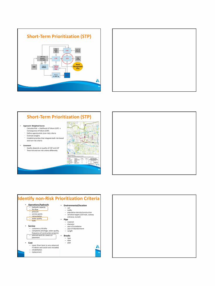
Short-Term Prioritization (STP)
• Approach: Weighted Scores
⁻ Calculate Risk = Likelihood of Failure (LOF) x
Consequence of Failure (COF)
⁻ Define opportunistic (non-risk) criteria
⁻ Estimate weights
⁻ Establish priorities that integrate both risk-based
and non-risk criteria
• Comment
⁻ Quality depends on quality of COF and LOF
⁻ Treat risk and non risk criteria differently
65
Identify non-Risk Prioritization Criteria• Operations/hydraulic
– hydraulic capacity– fire flow– pressure – service points– consumption– water quality– leaks
• Service – customers criticality– complaints (shortage, water quality,
frequency of construction projects)– planned work for sewers or
pavement
• Cost – repair (from basic to very advanced
if indirect and social costs included)– rehabilitation– replacement 66
• Environmental/location – soil– traffic– population density/construction– sensitive targets (rail track, subway
entrance, tunnel)
• Pipe– material– diameter– year of Installation– year of Abandonment– Length
• Breaks– type– date– pipe

Assign Prioritization Scores
67
Take handout 6
Aging Function/Effective Useful Live (EUL)
68
Aging Function/Effective Useful Live (EUL)⁻ Represents the break rate/average inspection score based on age⁻ One curve per pipe group
69
0
10
20
30
40
50
60
70
80
90
100
0 20 40 60 80 100 120
Bre
ak R
ate
Age
Break Rate based on Age
EUL =85 @ 40 brks/100 miles/yr

Aging Function/Effective Useful Live (EUL)Assumed
70
• Data Requirements/Tools: 2 points;EUL assumed, service level, Excel
• Plus: simple
• Minus: not precise; different utilitiesmay end up with same EULs.
Buried No Longer EUL Table
Service Level; assumed EUL
Current Break rate + age
Long-Term Plan (LTP)
71
Long-Term Plan Buried No Longer (BNL) - Level 1
• Approach– Determine R&R needs per year based on
assumed EULs
• Data and Tool requirements– Assumed EULs per cohort– Inventory – Cost data– Excel or BNL Tool
• Plus– Little data needed– Fast estimate
• Minus– Not utility-specific– Not linked to performance of system– Probably imprecise
72
Chart Legend
Water Mains
Sewers
WTP
WWTP
WW Lift Stations
Period
Average$/yr
Escalated*
* Average escalated annual R&R expenditure assuming
3% annual inflation
5 Year (09-13)
10 Year (09-18)
20 Year (09-28)
$1.1m
$1.1m
$1.4m
$/yr Non -
Escalated
$1.1m
$1.0m
$1.1m
$0
$500,000
$1,000,000
$1,500,000
$2,000,000
$2,500,000
$3,000,000
$3,500,000
$4,000,000
$4,500,000
2009 2010 2011 2012 2013 2014 2015 2016 2017 2018 2019 2020 2021 2022 2023 2024 2025 2026 2027 2028
Water Line Assets $96,597 $99,495 $102,48 $105,55 $108,72 $111,98 $613,70 $632,11 $651,07 $670,60 $560,90 $577,73 $595,06 $612,92 $631,30 $650,24 $91,835 $94,590 $97,428 $100,35
Water Treatment Plant Assets $972,68 $391,60 $0 $9,976 $6,447 $36,314 $154,95 $566,21 $110,88 $66,096 $178,49 $445,50 $40,579 $43,899 $43,050 $1,044, $106,56 $141,12 $27,426 $2,072,
Water Pump Station Assets $0 $0 $0 $0 $0 $0 $0 $0 $0 $0 $0 $0 $0 $0 $0 $0 $0 $0 $0 $0
Water Miscellaneous Assets $0 $0 $0 $0 $0 $0 $0 $0 $0 $0 $0 $0 $0 $0 $0 $0 $0 $0 $0 $0
Sewer Line Assets $3,076 $3,168 $3,263 $3,361 $3,462 $3,566 $9,544 $9,830 $10,125 $10,429 $6,608 $6,807 $7,011 $7,221 $7,438 $7,661 $1,123, $1,156, $1,191, $1,227,
Sewer Treatment Plant Assets $28,461 $2,193, $0 $306,89 $19,139 $0 $107,50 $477,72 $826,73 $21,020 $21,169 $407,09 $210,29 $16,429 $217,68 $153,94 $15,224 $434,32 $69,480 $186,12
Sewer Pump Station Assets $731,21 $22,124 $44,627 $129,09 $149,08 $76,779 $17,099 $33,022 $195,23 $165,82 $589,37 $929,66 $209,27 $212,92 $341,14 $276,08 $63,193 $109,46 $134,08 $235,40
Sewer Miscellaneous Assets $0 $0 $0 $0 $0 $0 $0 $0 $0 $0 $0 $0 $0 $0 $0 $0 $0 $0 $0 $0
Average $1,442, $1,442, $1,442, $1,442, $1,442, $1,442, $1,442, $1,442, $1,442, $1,442, $1,442, $1,442, $1,442, $1,442, $1,442, $1,442, $1,442, $1,442, $1,442, $1,442,
R&
R C
on
trib
uti
on
Fiscal Year
Annual R&R Contribution Requirement
Example LTP by pipe material

Level 2 - Advanced
73
• Approach
– LOF2: Failure/PC forecasting model (different for inspected and non-inspected pipes)
– COF2: Ranking tree or monetized
– STP2: LOF2 x COF2 or MCDMM
– EUL and aging function = drawn from statistics and forecasting model
– LTP = More advanced simulation tool (could be pipe-level and GIS-based)
• Plus
– No guessing of weights for LOF; model does it!
– Results at pipe level
– Better differentiation of LOF, COF, STP
– More utility-specific EULs and aging curves
• Minus
– Data needed at pipe level
– Data must be thoroughly cleaned-up (it could be a plus!)
– Minimum 5 yrs. of breaks; 10-25% of pipes inspected (depending)
– Software and expertise needed – look for interactive tool
Likelihood of Failure (LOF)
74
Likelihood of Failure (LOF)• Approach: Multivariable Regression Model
– Run descriptive statistics, calibrate and validate model
– Use model that takes all failure/PCA factors into account simultaneously
• Data Requirements/Tools
⁻ Pipe and environmental data (active –ACT- and, for
non-inspected, if available, abandoned –ABN-)
⁻ Breaks/inspection scores assigned to pipes
⁻ Statistical model/software
• Plus
- Can take RPLT (non-inspected pipes) into account
• Minus
⁻ Preliminary statistics and expertise to calibrate
model
75
0
10
20
30
0
0.2
0.4
0.6
1941
1945
1949
1953
1957
1961
1965
1969
1973
1977
1981
1985
1989
1993
1997
2001
Len
gth
(mi)
Bre
ak R
ate
(Nu
mb
er
Bre
aks/
mi/
yr.)
YOI
CI - Length and Break Rate based on Year of Installation
Weighted Break Rate Length
0
50
100
150
200
0
0.1
0.2
0.3
0.4
0.5
7
11 15 19 23 27 31 35 39 43 47 51 55 59 63 67 71
Len
gth
(mi)
Bre
ak R
ate
(Nu
mb
er
Bre
aks/
mi/
yr)
Age
CI 1942-2015 - Length and Yearly Break Rate based on Age at Year of Break
0
0.25
0.5
0.75
1
1.25
1.5
0
0.5
1
1.5
2
2.5
3
1985
1987
1989
1991
1993
1995
1997
1999
2001
2003
2005
2007
2009
2011
2013
2015
Len
gth
(m
i)
Bre
ak R
ate
(Nu
mb
er
Bre
aks/
mi/
yr.)
YOA
DI ABN - Length and Weighted Average YearlyBreak Rate up to YOA based on YOA
-0.5
0.5
1.5
2.5
3.5
4.5
-10.0
10.0
30.0
50.0
70.0
90.0
Sco
re
Len
gth
(mi)
MAT7
Length of Inspected Pipes, Average Age and Structural score based on MAT6
LENGTH INSPECTED AVE INSP AGE AVE SCORE PEAK
0
20
40
60
80
100
1
2
3
4
5
12 18 24 27 30 33 36 39 42 45 48 51 54 60 66 72 78 90 96
Len
gth
(mi)
/Ave
rage
Age
at I
nsp
ecti
on
Sco
re
DIAM
Length of Pipes (All and Inspected), Average Age at Inspectionand Structural Scores based on DIAM
AVE SCORE FEB 2016 PEAK 2016
AVE AGE AT INSP LENGTH INSPECTED PIPES

Example Results Non-inspected Pipes
76
FeatID NB BRKS YOI DIAM SOIL L COMMENTS LOF
439406 0 1960 12 BAD 0.001 SAME CO-VARIATES 0.00012 SAME LOF 5020359 0 1960 12 BAD 0.0011 SAME CO-VARIATES 0.00012 SAME LOF 414765 1 1960 12 BAD 0.0314 MORE BREAKS 0.01604 HIGHER LOF 423809 0 1960 12 BAD 0.0319 0.00135 396706 2 1948 6 BAD 0.0612 OLDER 0.08651 HIGHER LOF 379035 2 1967 6 BAD 0.0643 0.04741 438274 1 1953 4 BAD 0.0048 SMALLER DIAM 0.00544 HIGHER LOF 448483 1 1954 8 BAD 0.0044 0.00384 389358 1 1972 12 BAD 0.1847 WORSE SOIL 0.05209 HIGHER LOF 433341 1 1973 12 GOOD 0.1924 0.01721 379182 0 1960 12 4 0.27 LONGER 0.00757 HIGHER LOF 447565 0 1960 12 4 0.0137 0.00071
LOF
Output Results/Proxies for LOF: Predicted Break Number per pipe and per year
Example Results - Inspected PipesAnalytical Basis
77
Time t in years
Survival
probability S(t)
1
00
1
2
3p3(t)
p2(t)
p1(t)
S23(t)
S12(t)
ID Year p1 p2 p3 p4 p5 Lengthaggregated state
01000000006M-Central 2016 0.12 0.01 0.35 0.01 0.50 0.215 3.765
LOF: Aggregated Score = 1 x 0.12 + 2 x 0.01 + 3 x 0.35 + 4 x 0.01 + 5 x 0.5 = 3.77
Output Results/Proxies for LOF: probability to be in a certain state per pipe and per year
Example ResultsInspected Pipes
78
YOI Score Pred.
Year
1 2 3 4 5 Aggregat
ed Score
1930 1 10002000010M-10000000040M 2016 0.9751 0.0230 0.0018 0 0 1.0267
1930 1 10002000010M-10000000040M 2100 0.3230 0.0856 0.5878 0.0024 0.0012 2.2737
1960 1 20000000150M-20000000130M 2016 0.9681 0.0286 0.0032 0 0 1.0351
1960 1 20000000150M-20000000130M 2100 0.1734 0.0608 0.7583 0.0043 0.0032 2.6032
1994 1 06000000390M-06000000386M 2016 0.9495 0.0409 0.0095 0.0000 0 1.06
1994 1 06000000390M-06000000386M 2100 0.0038 0.0041 0.9562 0.0147 0.0211 3.0453
1930 3 11000000180M-11000000170M 2016 0 0 0.9924 0.0070 0.0006 3.0082
1930 3 11000000180M-11000000170M 2100 0 0 0.2015 0.1459 0.6526 4.4511
1960 3 05000000810M-TMP1513519M 2016 0 0 0.9920 0.0072 0.0008 3.0089
1960 3 05000000810M-TMP1513519M 2100 0 0 0.0122 0.0400 0.9478 4.9357
1994 3 05000000210M-05000000200M 2016 0 0 0.987 0.0096 0.0027 3.0151
1994 3 05000000210M-05000000200M 2100 0 0 0 0 1 5
1930 3 08000000020M-08000000009M 2016 0.1008 0.0099 0.3679 0.0049 0.5165 3.8264
1930 NA 08000000020M-08000000009M 2100 0.0517 0.0078 0.2750 0.0385 0.6270 4.1814
1960 NA TMP1447319M-TMP1447314M 2016 0.1426 0.0168 0.3831 0.0401 0.4175 3.5732
1960 NA TMP1447319M-TMP1447314M 2100 0.0671 0.0090 0.3421 0.0223 0.5596 3.9983

Consequence of Failure (COF)
79
Consequence of Failure (COF)
• Approaches
1. Ranking Tree (see next slide)
2. Monetized
⁻ Same but criteria are monetized
• Data Requirements/Tools
⁻ Impact criteria data
⁻ Excel/GIS
• Plus⁻ Real cost of break
• Minus⁻ Can be difficult to put price tag even on
indirect cost
80
Example Monetized Criteria
Criteria Category Criteria Low Moderate High Very High
Asset Repair Costs <$20K $20K - <$100K $100K - <$500K >$500K
Emergency Repair Costs <$20K $20K - <$100K $100K - <$500K >$500K
Asset Replacement Costs <$20K $20K - <$100K $100K - <$500K >$500K
Property Damage <$20K $20K - <$100K $100K - <$500K >$500K
Operational Losses (lost revenue, exporting to other facilities) <$20K $20K - <$100K $100K - <$500K >$500K
Economic Administrative and Legal Costs of Damage Settlements <$20K $20K - <$100K $100K - <$500K >$500K
Consultant/Engineering Services <$20K $20K - <$100K $100K - <$500K >$500K
Permit Violation yes
Environmental Environmental Regulatory Fine for Spills or Releases <$20K $20K - <$100K $100K - <$500K >$500K
Disruption of Service yes
Social Safety- Public and CWW staff yes
Magnitude Ranges for Triple Bottom Line Analysis
do not apply to safety
do not apply to permit violations
do not apply to safety
Ranking TreeApproach
⁻ Define TBL criteria
⁻ Set queries in GIS
⁻ High score rules with modifiers
Plus
⁻ Better differentiation in scores
Minus
⁻ Difficult to evaluate social and indirect costs
81

Short-Term Prioritization (STP)
82
Short-Term Prioritization (STP)
• Approaches:
• 1. Risk Score = LOF2 x COF2
• 2. Multi-Criteria Decision Making Model - for example
- Electre-Tri
⁻ Variables, criteria, weights
⁻ Reference profiles
• Data Requirements/Tools
⁻ COF and LOF
⁻ Opportunistic criteria data
⁻ Model/Software• Plus
⁻ Simple input files in excel⁻ No 1 x 100 = 10 x 10
• Minus⁻ Need special software⁻ Pipes assigned to priority categories. Ranking
difficult.
83
- a3 candidate for R&R- a8 not candidate for R&R- Model sorts out other pipes with less certain status
Example Electre-Tri Reference Profile
Aging FunctionEffective Useful Live (EUL)
84

Aging FunctionEffective Useful Live (EUL)
• Approach
– 2 options:
1. Plot historical break rate/score based on age at Year of Break (YOB) and extrapolate
1. Plot Predicted rate/score (LOF outputs)
– Set service level(s)
– Estimate EUL(s) from Aging Curve
85
Extrapolation – Cohort Level
86
0
0.02
0.04
0.06
0.08
0.1
0.12
0
10
20
30
40
50
60B
reak
Rat
e (N
um
ber
Bre
aks/
mi/
yr)
Age
DI - Length and Yearly Break Rate based on Age at YOB
Break Rate Linear (Break Rate)
0
0.05
0.1
0.15
0.2
0.25
0.3
0.35
0.4
0.45
0
10
20
30
40
50
60
70
80
Bre
ak R
ate
(Nu
mb
er B
reak
s/m
i/yr
)
Age
CI 1942-2015 - Length and Yearly Break Rate based on Age at Year of Break
0
0.5
1
1.5
2
2.5
3
3.5
4
4.5
5
1 11 21 31 41 51 61 71 81 91 101 111 121
Sco
re
Age
Score of Inspected Pipes based on Age
Non-inspected Pipes - PBNPipe or Cohort Level
0.000
0.025
0.050
0.075
0.100
0.125
0.150
0.175
0.200
32 36 40 44 48 52 56 60 64 68 72 76 80 84 88 92 96 100
Bre
ak R
ate
(brk
/mi/
yr)
Age
DI - Predicted Break Rate of ACT Pipes by Age (computed with PBNs)
0.00
0.05
0.10
0.15
0.20
0.25
0.30
0.35
0.40
0.45
0.50
0.55
0.60
51 53 55 57 59 61 63 65 67 69 71 73 75 77 79 81 83 85 87 89 91 93 95 97 99
Bre
ak R
ate
(brk
/mi/
yr)
Age
CI - Predicted Break Rate of ACT Pipes by Age (computed with PBNs)
59 86
0.40
0.25
Low COF BR= 0.25Medium COF BR = 0.4
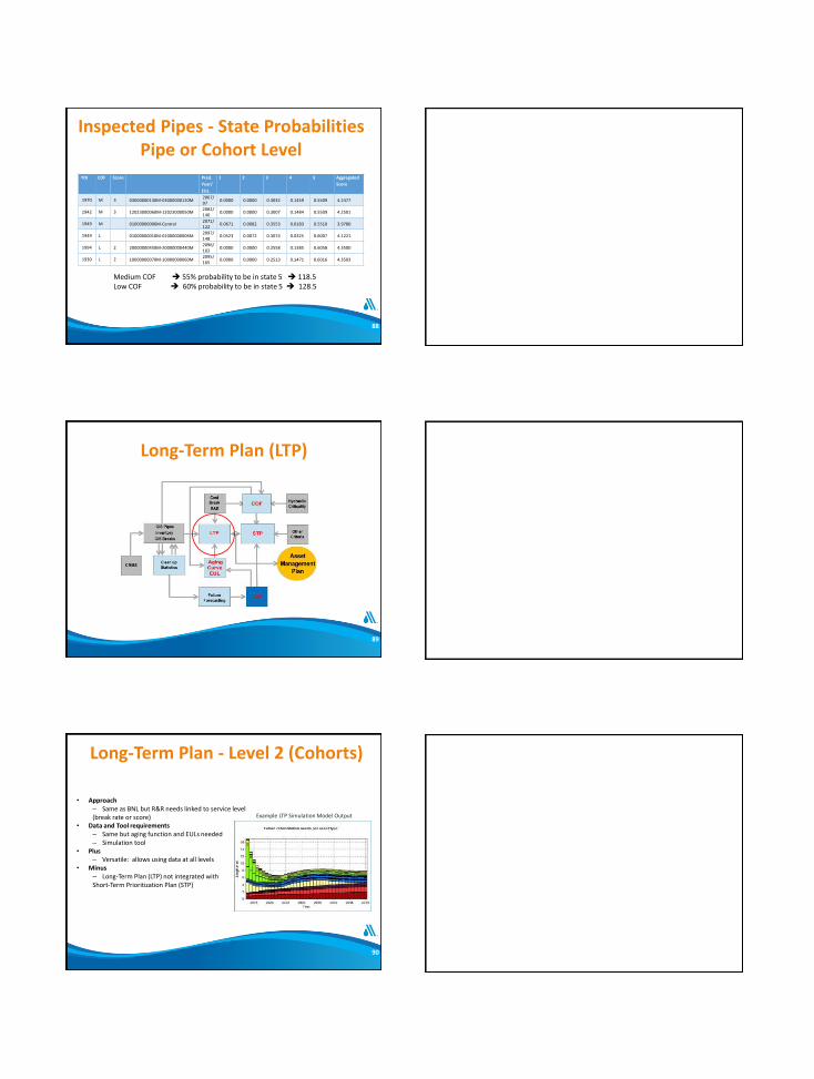
Inspected Pipes - State ProbabilitiesPipe or Cohort Level
88
YOI COF Score Pred.
Year/
EUL
1 2 3 4 5 Aggregated
Score
1970 M 3 03000000130M-03000000120M2067/97
0.0000 0.0000 0.3032 0.1459 0.5509 4.2477
1942 M 3 12023000060M-12023000050M2082/140
0.0000 0.0000 0.3007 0.1484 0.5509 4.2501
1949 M 01000000006M-Central2071/122
0.0671 0.0082 0.3553 0.0183 0.5510 3.9780
1949 L 01000000010M-01000000006M2097/148
0.0523 0.0072 0.3074 0.0325 0.6007 4.1221
1994 L 2 20000000450M-20000000440M2096/102
0.0000 0.0000 0.2558 0.1385 0.6058 4.3500
1930 L 2 10000000070M-10000000060M2095/165
0.0000 0.0000 0.2513 0.1471 0.6016 4.3503
Medium COF 55% probability to be in state 5 118.5Low COF 60% probability to be in state 5 128.5
Long-Term Plan (LTP)
89
Long-Term Plan - Level 2 (Cohorts)
• Approach– Same as BNL but R&R needs linked to service level (break rate or score)
• Data and Tool requirements– Same but aging function and EULs needed– Simulation tool
• Plus– Versatile: allows using data at all levels
• Minus– Long-Term Plan (LTP) not integrated with Short-Term Prioritization Plan (STP)
90
Example LTP Simulation Model Output
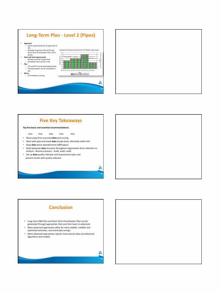
Long-Term Plan - Level 2 (Pipes)
• Approach– Same as previously but at pipe level in
GIS– Develop Long-Term Plan (LTP) and
Short-Term Prioritization Plan (STP) jointly
• Data and Tool requirements– All data must be at pipe level– Simulation tool can be in GIS
• Plus– LTP and STP can be developed jointly– Priority projects can be visualized in
GIS • Minus
– STP limited to scoring
91
Example GIS-based and pipe-level LTP Model using output
Five Key TakeawaysTop five basic and essential recommendations:
• Move away from assumed data and scoring
• Work with pipe and break data at pipe level, ultimately within GIS
• Keep data about abandonment (ABN pipes)
• Build adequate data structure throughout organization from collection to analysis - Business process - Audit, audit, audit
• Set up data quality indicator and improvement plan and
present results with quality indicator
92
DataData Data Data Data
Conclusion
• Long-Term R&R Plan and Short-Term Prioritization Plan can be generated through approaches that vary from basic to advanced.
• More advanced approaches allow for more reliable, credible and optimized estimates, and eventually savings.
• More advanced approaches require more precise data and advanced algorithms and models.
93

09:00-9:05Welcome
Annie
9:05-9:15
Introduction
Kevin
9:15-9:20
Introduction Questionnaire
Kevin
9:20-9:40
AM Framework and Data
Kurt
9:40-10:30
Data clean-up Exercises
Annie et al
10:30-10:40
BREAK
10:40-11:40
Analytical Approach – From Basic to Advanced –
Non-inspected and Inspected Pipes
Annie and Celine
11:40-12:00
Case Study: Columbus – From Basic to Advanced Approach
Non-inspected Pipes
Kevin
1:00-1:10
Q/A about Columbus
Kevin
1:10-1:40
Case Study: Dallas – From Basic to Advanced Approach
Inspected Pipes
Celine and Annie
1:40-2:40
Group Discussion
Where do you stand? Celine
Where do you want to go? Kurt
2:40-2:50
BREAK
2:50-3:00
Synthesis of Previous Discussion
Kevin
3:00-3:25
Mixing Analytical Approach and Inspection Program
Annie
3:25-3:55
Case Study: AWWU – From Basic to Advanced Approach
Mixing Analytical Approach with Inspection Program
Kurt
3:55-4:00 Wrap-up
Annie
94
12:00-1:00LUNCH
Workshop Agenda
Lunch
95
09:00-9:05Welcome
Annie
9:05-9:15
Introduction
Kevin
9:15-9:20
Introduction Questionnaire
Kevin
9:20-9:40
AM Framework and Data
Kurt
9:40-10:30
Data clean-up Exercises
Annie et al
10:30-10:40
BREAK
10:40-11:40
Analytical Approach – From Basic to Advanced –
Non-inspected and Inspected Pipes
Annie and Celine
11:40-12:00
Case Study: Columbus – From Basic to Advanced Approach
Non-inspected Pipes
Kevin
1:00-1:10
Q/A about Columbus
Kevin
1:10-2:10
Group Discussion
Where do you stand? Where do you want to go?
Celine, Kevin, Kurt
2:10-2:20
Synthesis of Previous Discussion
Kevin
2:20-2:50
Mixing Analytical Approaches and Inspection Program
Annie
2:50-3:00
BREAK
3:00-3:25
Case Study: AWWU – From Basic to Advanced Approach
Mixing Analytical Approach with Inspection Program
Kurt
3:25-3:50
Case Study: Dallas – From Basic to Advanced Approach
Inspected Pipes
Celine and Annie
3:50-4:00 Wrap-up
96
12:00-1:00LUNCH

09:00-9:05Welcome
Annie
9:05-9:15
Introduction
Kevin
9:15-9:20
Introduction Questionnaire
Kevin
9:20-9:40
AM Framework and Data
Kurt
9:40-10:30
Data clean-up Exercises
Annie et al
10:30-10:40
BREAK
10:40-11:40
Analytical Approach – From Basic to Advanced –
Non-inspected and Inspected Pipes
Annie and Celine
11:40-12:00
Case Study: Columbus – From Basic to Advanced Approach
Non-inspected Pipes
Kevin
1:00-1:10
Q/A about Columbus
Kevin
1:10-1:40
Case Study: Dallas – From Basic to Advanced Approach
Inspected Pipes
Celine and Annie
1:40-2:40
Group Discussion
Where do you stand? Celine
Where do you want to go? Kurt
2:40-2:50
BREAK
2:50-3:00
Synthesis of Previous Discussion
Kevin
3:00-3:25
Mixing Analytical Approach and Inspection Program
Annie
3:25-3:55
Case Study: AWWU – From Basic to Advanced Approach
Mixing Analytical Approach with Inspection Program
Kurt
3:55-4:00 Wrap-up
Annie
97
12:00-1:00LUNCH
Workshop Agenda
09:00-9:05Welcome
Annie
9:05-9:15
Introduction
Kevin
9:15-9:20
Introduction Questionnaire
Kevin
9:20-9:40
AM Framework and Data
Kurt
9:40-10:30
Data clean-up Exercises
Annie et al
10:30-10:40
BREAK
10:40-11:40
Analytical Approach – From Basic to Advanced –
Non-inspected and Inspected Pipes
Annie and Celine
11:40-12:00
Case Study: Columbus – From Basic to Advanced Approach
Non-inspected Pipes
Kevin
1:00-1:10
Q/A about Columbus
Kevin
1:10-1:40
Case Study: Dallas – From Basic to Advanced Approach
Inspected Pipes
Celine and Annie
1:40-2:40
Group Discussion
Where do you stand? Celine
Where do you want to go? Kurt
2:40-2:50
BREAK
2:50-3:00
Synthesis of Previous Discussion
Kevin
3:00-3:25
Mixing Analytical Approach and Inspection Program
Annie
3:25-3:55
Case Study: AWWU – From Basic to Advanced Approach
Mixing Analytical Approach with Inspection Program
Kurt
3:55-4:00 Wrap-up
Annie
98
12:00-1:00LUNCH
Workshop Agenda
Questionnaire
• Take handout 1
99

Break
100
09:00-9:05Welcome
Annie
9:05-9:15
Introduction
Kevin
9:15-9:20
Introduction Questionnaire
Kevin
9:20-9:40
AM Framework and Data
Kurt
9:40-10:30
Data clean-up Exercises
Annie et al
10:30-10:40
BREAK
10:40-11:40
Analytical Approach – From Basic to Advanced –
Non-inspected and Inspected Pipes
Annie and Celine
11:40-12:00
Case Study: Columbus – From Basic to Advanced Approach
Non-inspected Pipes
Kevin
1:00-1:10
Q/A about Columbus
Kevin
1:10-1:40
Case Study: Dallas – From Basic to Advanced Approach
Inspected Pipes
Celine and Annie
1:40-2:40
Group Discussion
Where do you stand? Celine
Where do you want to go? Kurt
2:40-2:50
BREAK
2:50-3:00
Synthesis of Previous Discussion
Kevin
3:00-3:25
Mixing Analytical Approach and Inspection Program
Annie
3:25-3:55
Case Study: AWWU – From Basic to Advanced Approach
Mixing Analytical Approach with Inspection Program
Kurt
3:55-4:00 Wrap-up
Annie
101
12:00-1:00LUNCH
Workshop Agenda
AWWA Progress in AM Survey Results (2015)
• 550 Utilities Responded
• 59% serve less than 50,000 customers; 15% serve over 500,000
• 91% public; 9% private
• 85% retail; 45% wholesale
• 29% have part- or full-time AM staff
102

103
104
105

106
107
108

109
09:00-9:05WelcomeAnnie
9:05-9:15Introduction Kevin
9:15-9:20Introduction QuestionnaireKevin
9:20-9:40AM Framework and DataKurt
9:40-10:30Data Clean up ExercisesAnnie et al
10:30-10:40BREAK
10:40-11:40Analytical Approach – From Basic to Advanced Approach Non Inspected and Inspected PipesAnnie and Celine
11:40-12:00Case Study: Columbus – From Basic to Advanced ApproachNon Inspected PipesKevin
1:00-1:10Q/A about ColumbusKevin
1:10-1:40Case Study: Dallas – From Basic to Advanced Approach Inspected PipesCeline and Annie
1:40-2:40Group DiscussionWhere do you stand? CelineWhere do you want to go? Kurt
2:40-2:50BREAK
2:50-3:00Synthesis of Previous DiscussionKevin
3:00-3:25 Mixing Analytical Approach and Inspection ProgramAnnie
3:25-3:55Case Study: AWWU – From Basic to Advanced Approach Mixing Analytical Approach with Inspection ProgramKurt
3:55-4:00 Wrap-upAnnie
Workshop Agenda12:00-1:00LUNCH
EUL Estimation - ApproachesCost versus Precision
> >Lab
CouponLimited number
of pipes
PCAhydrant to hydrantAverage thickness
Limited length
Analytical ApproachesPipe, cohort
Whole system
110
PCA in a Cost Efficient AM Plan
• Example:
– 2,000 mi
– $ 0.8M budget allocated for PCA in 2016
– PCA $20,000/mi
– We can do 40 mi = 2% of system
• What is the purpose of the PCA?
• Can a certain purpose be accomplished with 2%?
• What purpose can be accomplished with 2%
• How much money is needed to accomplish a certain purpose ?
• What pipes should be inspected to accomplish a certain purpose with a given budget?
111

Why conducting PCA?
1. Justify investment: Evaluate PCA of pipes with high Risk Score to decide whether they should be replaced
2. Validate and improve aging curves and EULs generated using analytical approaches (basic or, preferably, advanced)
3. Generate aging curves and EULs for pipe groups with few breaks but high COF (like large pipesfor example)
Are we trying to generate results to answer a punctual question, e.g., ‘should pipe be replaced this year?’, or, for optimal cost efficiency when building an R&R & Inspection Plan?
112
Suggestion
Using a combination of analytical approaches along with PCA will lead
to more cost-efficiency but this requires a plan!
+ =Saving
113
Level of Cost of PCA
1. Risk scores have been produced using basic or advanced approaches; pipes have been prioritized for replacement based on their risk score.
PURPOSE OF PCA: justify R&R investment
PCA $ depends on length of high risk pipes (vice versa if PCA $ is limited, focus shouldbe on highest risk pipes)
114
Risk Score = COF x LOF
Based on purpose, data availability and type of analytical approach used performed
3 different situations

2. A lot of breaks; good LOF and aging curves have been generated using advanced analytical approaches
PURPOSE OF PCA: validate aging curves and analytical results
PCA $ depends on statistically significant size of the sample
3. No break; no inspection data; access to PCA/LOF forecasting model
PURPOSE OF PCA: conduct a PCA program on a sample of the pipes in order to extrapolate to overall group of “similar pipes” and have PCA/LOF score for every pipe and in the future
PCA $ depends on statistically significant size of the sample
115
ZscoreStdDev
margin of errorpopulation size
Level of Cost of PCA (Cont’d)
Sample size out of a certain cohort’s population?
Intuitively (and mathematically) sample size depends on:
• How much, when conducting multiple measurements on a population (of individuals who behave “similarly” within a certain range), the results vary (average variation is the standard deviation) - If we want StdDev to be small we need to get a population with very similar degradation pattern (descriptive statistics will help do that).
• How much + or – error we can tolerate in the measurement (margin of error/confidence interval).
• How confident (90%? 95%, 99%?) we want to be that the actual mean of the future measurement on the sample would fall within the confidence interval (expressed by the Z score - published statistical tables).
• Population from which sample is extracted. A population twice as big does not require a sample twice bigger.
116
Example
Level of
confidenceZ score StdDev
Margin of error+/-
Sample size
95% 1.96 0.5 15.2% 40
90% 1.64 0.5 12.7% 40
• Fixed:- StdDev for a certain cohort and PCA technology (here 50% = .5) - Budget: we only have money for 40 mi out of a 1,000-mi population of pipes.
• If we want:- 95% confidence margin of error will be 15.2%.- 90% confidence margin of error will go down to 12.7%
117

The smaller the population of reference the larger the proportion between sample size and that population. For previous example for same statistical performance (Confidence and Error):- If population of reference is 1,000 miles, sample size must be around 40 mi- If population of reference is 100 miles, sample size must be around 29 mi- If population of reference is of any size above 1,000 mi, the requested sample size
remains close to 40 mi
PopulationConfidence Interval
StdDevMargin of Error
Sample Size
100 95% 0.50 0.153 29.3
500 95% 0.50 0.153 38
1,000 95% 0.50 0.153 39.5
2,000 95% 0.50 0.153 40.2
3,000 95% 0.50 0.153 40.5
4,000 95% 0.50 0.153 40.6
5,000 95% 0.50 0.153 40.7
Looks positive but in reality it is difficult to have small StdDev with very large population.
So solution is not to shoot for large cohorts
118
Example of a cost efficient plan
– 2,000 mi
– $ 800,000 budget allocated for PCA in 2016 and every year
– PCA $20,000/mi
– Budget for 40 mi/yr. = 2% of system
– Challenge is to get good estimate of StdDev which depends on coherence of the cohort. The fewer the number of breaks, the more difficult it is to get smaller StdDev.
119
AC Pipes2,000 miles / 850 breaks / 4 brk-100 mi-yr.
Type I | AC (<=1956)306 brks / 12 mi / 254 mi)
10.2 brk-100 mi-yr
Type || AC (>=1957)566 brks / 26 mi / 1,874 mi
3.2 brk-100 mi-yr
Small<=6154 brks
6.4 mi73 mi
19.2 b-r
Med 8-14154 brks
5.5 mi108 mi
11.2 b-rate
Large >=160 brks0 mi4 mi
0 b-rate
Small<=6194 brks
8.8 mi688 mi4.8 b-r
Med 8-14350 brks15.5 mi
1,342 mi2 b-rate
Large >=1622 brks0.3 mi188 mi
0.8 b-rate
First Year
• Use PCA to estimate the Likelihood Of Failure (LOF) and aging curve of the pipes that belong to a cohort with few breaks (below, the large pipes) for which statistical analysis is not possible.
• If we spend our $0.8M on PCA for large pipes (pop of 192 miles) we could have a sample size of 40 mi. Given a StdDev of 0.5 we could have a margin of error of 13.8% and a confidence interval of 95%. We can then use PCA forecasting model to compute LOF and risk score of every large pipe and select priority pipes for inspection in subsequent years.
• On medium and small size pipes there are typically enough breaks to generate LOF, agingcurves and EUL out of failure statistics.
Small<=6154 brks
6.4 mi73 mi
19.2 b-r
Med 8-14154 brks
5.5 mi108 mi
11.2 b-rate
Large >=160 brks0 mi4 mi
0 b-rate
Small<=6194 brks
8.8 mi688 mi4.8 b-r
Med 8-14350 brks15.5 mi
1,342 mi2 b-rate
Large >=1622 brks0.3 mi188 mi
0.8 b-rate
120

Subsequent years• Inspect large pipes as determined by risk score.
• In addition, based on remaining budget, inspect small and medium pipes in order of prioritydetermined by risk score. If we consider 4 different cohorts (73, 108, 688 and 1,342 mi) and we want same stat performance (StdDev = 0.5 TBC-large cohorts may have a bigger stdDev, margin of error = 10%, confidence interval = 95%) we will need to conduct PCA on 41 (57%) + 51 (47%) + 84(12%) + 90 (7%) = 266 (12% total) miles; which could be achieved in 6.5 years at a cost of $ 5.3 M.
• Then PCA failure forecasting model could be used for small and medium pipes to obtain LOF (and risk score) for each pipe and each year.
• Using LOF and risk scores as well as cost data, decide at what point pipes should be re-inspected or just rehabilitated or replaced.
121
Small<=6154 brks
6.4 mi73 mi
19.2 b-r
Med 8-14154 brks
5.5 mi108 mi
11.2 b-rate
Large >=160 brks0 mi4 mi
0 b-rate
Small<=6194 brks
8.8 mi688 mi4.8 b-r
Med 8-14350 brks15.5 mi
1,342 mi2 b-rate
Large >=1622 brks0.3 mi188 mi
0.8 b-rate
Conclusion
This requires:
- planning ahead including purpose of the PCA program
- Adoption of advanced analytical approaches
+ =Saving
122
09:00-9:05Welcome
Annie
9:05-9:15
Introduction
Kevin
9:15-9:20
Introduction Questionnaire
Kevin
9:20-9:40
AM Framework and Data
Kurt
9:40-10:30
Data clean-up Exercises
Annie et al
10:30-10:40
BREAK
10:40-11:40
Analytical Approach – From Basic to Advanced –
Non-inspected and Inspected Pipes
Annie and Celine
11:40-12:00
Case Study: Columbus – From Basic to Advanced Approach
Non-inspected Pipes
Kevin
1:00-1:10
Q/A about Columbus
Kevin
1:10-1:40
Case Study: Dallas – From Basic to Advanced Approach
Inspected Pipes
Celine and Annie
1:40-2:40
Group Discussion
Where do you stand? Celine
Where do you want to go? Kurt
2:40-2:50
BREAK
2:50-3:00
Synthesis of Previous Discussion
Kevin
3:00-3:25
Mixing Analytical Approach and Inspection Program
Annie
3:25-3:55
Case Study: AWWU – From Basic to Advanced Approach
Mixing Analytical Approach with Inspection Program
Kurt
3:55-4:00 Wrap-up
Annie
123
12:00-1:00LUNCH
Workshop Agenda

09:00-9:05Welcome
Annie
9:05-9:15
Introduction
Kevin
9:15-9:20
Introduction Questionnaire
Kevin
9:20-9:40
AM Framework and Data
Kurt
9:40-10:30
Data clean-up Exercises
Annie et al
10:30-10:40
BREAK
10:40-11:40
Analytical Approach – From Basic to Advanced –
Non-inspected and Inspected Pipes
Annie and Celine
11:40-12:00
Case Study: Columbus – From Basic to Advanced Approach
Non-inspected Pipes
Kevin
1:00-1:10
Q/A about Columbus
Kevin
1:10-1:40
Case Study: Dallas – From Basic to Advanced Approach
Inspected Pipes
Celine and Annie
1:40-2:40
Group Discussion
Where do you stand? Celine
Where do you want to go? Kurt
2:40-2:50
BREAK
2:50-3:00
Synthesis of Previous Discussion
Kevin
3:00-3:25
Mixing Analytical Approach and Inspection Program
Annie
3:25-3:55
Case Study: AWWU – From Basic to Advanced Approach
Mixing Analytical Approach with Inspection Program
Kurt
3:55-4:00 Wrap-up
Annie
124
12:00-1:00LUNCH
Workshop Agenda