The potential of small unmanned aircraft systems and structure-from-motion 1

for topographic surveys: A test of emerging integrated approaches at Cwm 2

Idwal, North Wales 3

T.N.Tonkina1, N.G.Midgleya , D.J.Grahamb, J.C.Labadza 4

5

aSchool of Animal, Rural and Environmental Sciences, Nottingham Trent University, 6

Brackenhurst Campus, Southwell, Nottinghamshire NG25 0QF, UK 7

8

bPolar and Alpine Research Centre, Department of Geography, Loughborough 9

University, Leicestershire LE11 3TU, UK 10

11

1Corresponding author. Tel.: + 44 115 848 5257. toby.tonkin@ntu.ac.uk 12

13

Abstract 14

Novel topographic survey methods that integrate both structure-from-motion (SfM) 15

photogrammetry and small unmanned aircraft systems (sUAS) are a rapidly evolving 16

investigative technique. Due to the diverse range of survey configurations available 17

and the infancy of these new methods, further research is required. Here, the 18

accuracy, precision and potential applications of this approach are investigated. A 19

total of 543 images of the Cwm Idwal moraine-mound complex were captured from a 20

light (< 5 kg) semi-autonomous multi-rotor unmanned aircraft system using a 21

consumer-grade 18 MP compact digital camera. The images were used to produce a 22

DSM (digital surface model) of the moraines. The DSM is in good agreement with 23

7761 total station survey points providing a total vertical RMSE value of 0.517 m and 24

vertical RMSE values as low as 0.200 m for less densely vegetated areas of the 25

DSM. High-precision topographic data can be acquired rapidly using this technique 26

with the resulting DSMs and orthorectified aerial imagery at sub-decimetre 27

resolutions. Positional errors on the total station dataset, vegetation and steep terrain 28

are identified as the causes of vertical disagreement. Whilst this aerial survey 29

approach is advocated for use in a range of geomorphological settings, care must be 30

taken to ensure that adequate ground control is applied to give a high degree of 31

accuracy. 32

33

Highlights 34

An integrated sUAS and SfM approach is used to generate high-resolution 35

topographic data. 36

SfM data compared with a total station ground survey. 37

Positional errors on the total station dataset, vegetation and steep terrain are 38

identified as causes of vertical difference between the two datasets. 39

The integration of a combined sUAS and SfM approach is discussed. 40

41

Keywords 42

Small unmanned aircraft system, Structure from motion, Digital surface model, 43

Digital elevation model, Topographic surveying 44

1 Introduction 45

The use of small unmanned aircraft systems (sUAS) and structure-from-motion 46

(SfM) digital photogrammetry presents a new methodological frontier for topographic 47

data acquisition and is of interest to scientists researching in a range of 48

geomorphological environments (Westoby et al., 2012; Carrivick et al., 2013; 49

Hugenholtz et al., 2013; Tarolli, 2014). Traditionally low-level aerial photography has 50

been acquired using a variety of unmanned platforms including small lighter-than-air 51

blimps, kites, and model fixed-wing and single rotor aircraft (e.g. Wester-52

Ebbinghaus, 1980; Rango et al., 2009; Smith et al., 2009; Hugenholtz et al., 2013). 53

More recently lightweight (< 5 kg), relatively low-cost multi-rotor aerial platforms have 54

been used to capture low-level imagery (Harwin and Lucieer, 2012; Niethammer et 55

al., 2012; Rosnell and Honkavaara, 2012; Mancini et al., 2013; Lucieer et al., 2014). 56

These sUAS can be programmed to fly semi-autonomously at fixed altitudes along 57

flight lines, ensuring optimal image overlap for digital photogrammetry. A key 58

strength of the integrated sUAS–SfM approach is the degree of automation involved. 59

Previously, a high degree of user experience was a prerequisite for both the 60

operation of aerial platforms and the application of photogrammetric methods to 61

extract meaningful topographic data from aerial imagery (Aber et al., 2010). The 62

premise of SfM as a digital photogrammetric technique is that three-dimensional 63

coordinates can be extracted from sufficiently overlapping photography without the 64

need for camera spatial information (Snavely et al., 2008; Westoby et al., 2012). The 65

integration of SfM with sUAS camera platforms offers a rapid and increasingly cost 66

effective option for geomorphologists to produce digital surface models (DSMs), with 67

resolution and data quality proposed to be on-par with, or better than LiDAR 68

(Carrivick et al., 2013; Fonstad et al., 2013). SfM based topographic surveys have 69

recently been used for a variety of geoscientific applications including quantifying 70

rates of landslide displacement (Lucieer et al., 2013), mapping vegetation spectral 71

dynamics (Dandois and Ellis, 2013), producing DEMs (digital elevation models) of 72

agricultural watersheds (Ouédraogo et al., 2014), quantifying coastal erosion rates 73

(James and Robson, 2012), and measuring rates of glacier motion and thinning 74

(Whitehead et al., 2013). The potential of SfM to aid geomorphological mapping, 75

derive measurements of landforms (morphometry) and quantify geomorphological 76

change is evident. Numerous software packages for SfM are now available and 77

include cloud-based processing, which has the additional benefit of not requiring a 78

high-specification consumer computer capable of handling the image processing. 79

80

Whilst a range of recent studies have sought to quantify data quality and associated 81

error of SfM techniques (Harwin and Lucieer, 2012; Turner et al., 2012; Westoby et 82

al., 2012; Dandois and Ellis, 2013; Fonstad et al., 2013; Hugenholtz et al., 2013; 83

Ouédraogo et al., 2014), further research is beneficial due to the diverse nature of 84

the aerial platforms and consumer-grade digital cameras available for the production 85

of topographic data using this methodology. Existing reports on the effectiveness of 86

integrated multi-rotor based sUAS–SfM approaches describe surveys conducted 87

from relatively low altitudes (< 50 m). The aims of this research are to: (1) provide a 88

systematic account of the data acquisition process associated with this new 89

integrated technique; (2) compare vertical spot heights obtained from the sUAS–SfM 90

survey to those obtained from a total station ground survey; (3) highlight important 91

considerations for researchers seeking to use sUAS and SfM approaches to acquire 92

data for topographic investigations; and (4) provide a baseline for the potential 93

spatial resolutions when using a consumer-grade 18 MP compact digital camera at a 94

target flight altitude of 100 m. 95

96

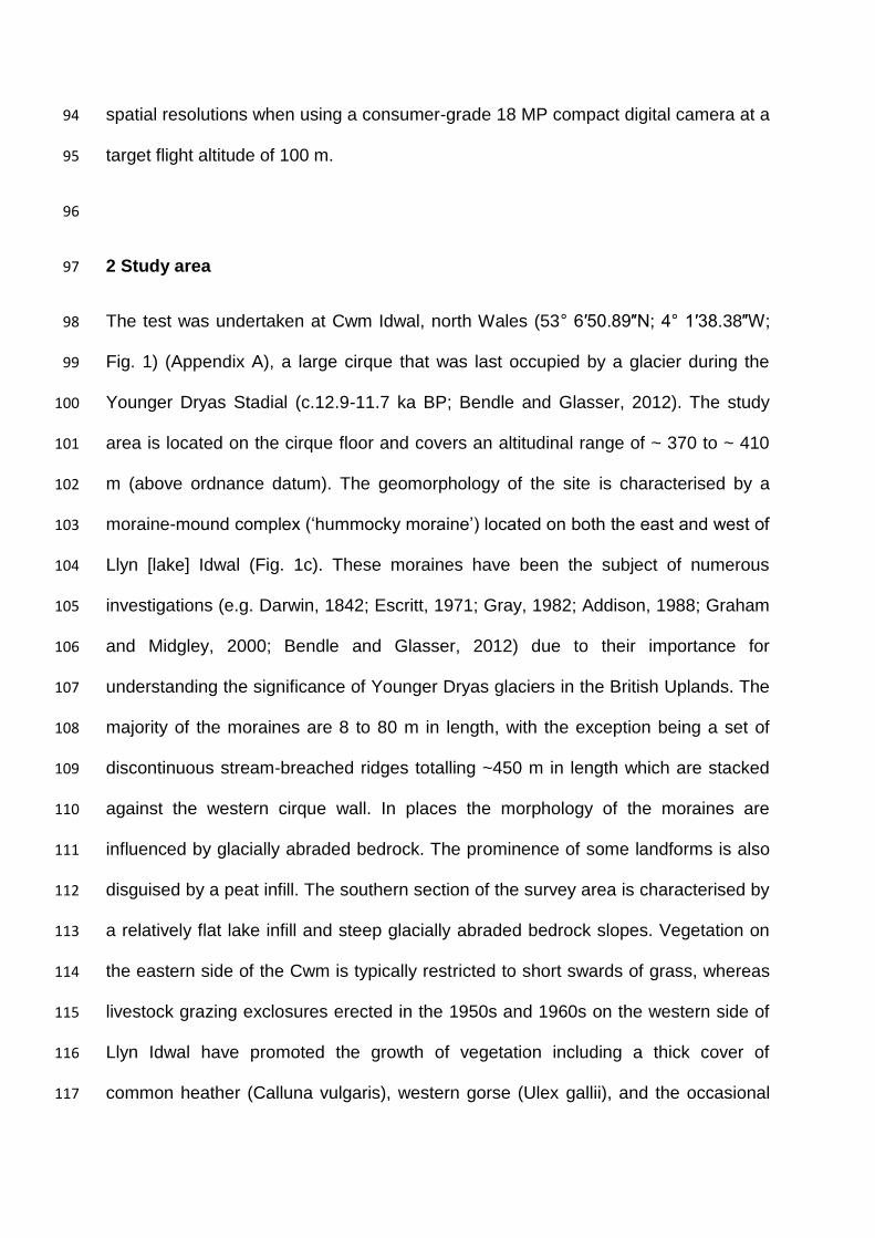
2 Study area 97

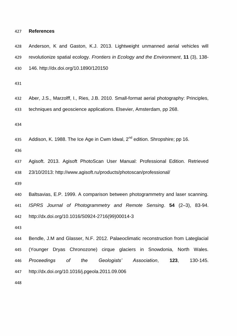
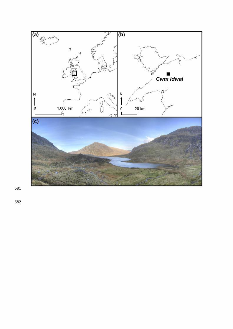
The test was undertaken at Cwm Idwal, north Wales (53° 6′50.89″N; 4° 1′38.38″W; 98

Fig. 1) (Appendix A), a large cirque that was last occupied by a glacier during the 99

Younger Dryas Stadial (c.12.9-11.7 ka BP; Bendle and Glasser, 2012). The study 100

area is located on the cirque floor and covers an altitudinal range of ~ 370 to ~ 410 101

m (above ordnance datum). The geomorphology of the site is characterised by a 102

moraine-mound complex (‘hummocky moraine’) located on both the east and west of 103

Llyn [lake] Idwal (Fig. 1c). These moraines have been the subject of numerous 104

investigations (e.g. Darwin, 1842; Escritt, 1971; Gray, 1982; Addison, 1988; Graham 105

and Midgley, 2000; Bendle and Glasser, 2012) due to their importance for 106

understanding the significance of Younger Dryas glaciers in the British Uplands. The 107

majority of the moraines are 8 to 80 m in length, with the exception being a set of 108

discontinuous stream-breached ridges totalling ~450 m in length which are stacked 109

against the western cirque wall. In places the morphology of the moraines are 110

influenced by glacially abraded bedrock. The prominence of some landforms is also 111

disguised by a peat infill. The southern section of the survey area is characterised by 112

a relatively flat lake infill and steep glacially abraded bedrock slopes. Vegetation on 113

the eastern side of the Cwm is typically restricted to short swards of grass, whereas 114

livestock grazing exclosures erected in the 1950s and 1960s on the western side of 115

Llyn Idwal have promoted the growth of vegetation including a thick cover of 116

common heather (Calluna vulgaris), western gorse (Ulex gallii), and the occasional 117

rowan (Sorbus aucuparia) and silver birch (Betula pendala) (Rhind and Jones, 118

2003). A large part of the moraine-mound complex and surrounding area were 119

surveyed with a total station by Graham and Midgley (2000). A similar area was 120

surveyed by a sUAS to allow a direct comparison between total station based data 121

acquisition, and the sUAS–SfM method used for this study. 122

123

3 Methods and materials 124

3.1 Image Image and data acquisition 125

Aerial imagery was acquired using a Canon EOS-M 18 MP camera suspended from 126

a DJI S800 Hexacopter (Fig. 2). A Photohigher AV130 servo driven gimbal 127

maintained the camera angle close to the nadir. The hexacopter was equipped with 128

a Wookong-M GPS assisted flight controller which allowed for semi-autonomous 129

surveys. Survey flight-lines were pre-programmed via the DJI Ground-Station 130

software package. For all surveys the sUAS was set to a target altitude of 100 m 131

above ground level (AGL) and horizontal ground speed of 2.5 ms-1. The target 132

altitude is calculated in the DJI Ground-Station software using elevation data derived 133

from Google Earth. Parallel flights lines were programmed to have an image sidelap 134

of 80%, whilst taking into account the camera sensor size (22.3 × 14.9 mm) and 135

focal length (22 mm). The intervalometer function of the Magic Lantern third-party 136

camera firmware was set to acquire imagery every 2 s along parallel flight lines. 137

Actual image acquisition was every ~ 4 s, resulting in image capture approximately 138

every 10 m along flight lines. Although image capture can be triggered using the DJI 139

flight controller, an intervalometer was used for its improved reliability and potential 140

to capture excess imagery along flight lines. This allowed for blurred or poor quality 141

imagery to be removed whilst ensuring that an image onlap in excess of 80% was 142

maintained. The camera was set to shutter-priority mode and used a 1/1000 s 143

shutter speed. To provide the required image coverage the survey area had to be 144

split between four flights. The sUAS had a flight-time of ~ 14 min whilst carrying its 145

payload (using an 11 Ah, 22.2 V, 6 cell lithium polymer battery). A generous 146

overhead (~ 2 min) was left in order to safely land the sUAS. In the UK unaided 147

visual line of sight (VLOS) has to be maintained whilst operating sUAS (CAA, 2012). 148

Therefore the ground equipment and launch position were moved between flights to 149

allow the sUAS to be easily observed, and manually controlled if necessary. 150

151

The total station dataset was acquired over multiple survey sessions in 1997 and 152

1998 using a Leica TC600 (Graham and Midgley, 2000). An assessment of error for 153

this data set is unavailable. However, measurement accuracies (expressed as 154

standard deviation) for the TC600 are defined by Leica (1997), with distance 155

measurements accurate to 2 mm ± 2 ppm and angle (horizontal and vertical) 156

measurements to 1.5 mgon. As the original total station dataset was collected for 157

the purpose of characterising the overall shape of the moraine-mound complex, 158

individual points were collected rapidly. Points recorded whilst the prism pole was 159

not perfectly vertical have the potential to result in misregistration between the two 160

datasets. The extent of the resulting error will be exacerbated by slope steepness 161

and the height of the reflector on the detail pole. The SfM dataset was tied into the 162

same arbitrary co-ordinate system and datum through the use of two brass pin 163

benchmarks located on exposed bedrock on the east and west of Llyn Idwal. Point 164

densities for the validation points reach as high as 20 per 100 m2 over the moraine-165

mound complex (Graham and Midgley, 2000). For the sUAS survey, 19 SfM ground-166

control points (GCPs) were distributed across the survey area (Fig. 3a). White 167

laminated A3 size targets (297 × 420 cm) were used as GCPs and were found to be 168

adequately visible on the aerial imagery. These GCPs were surveyed with a Leica 169

TC407 total station to a precision of ≤ 1 mm and estimated accuracy of < 3 cm. 170

171

3.2 Image processing and analysis 172

From the original set of 824 images, 543 images were selected for model 173

reconstruction using the Agisoft Photoscan 1.0.0 (build 1795) software package. 174

Images were visually assessed for quality and blurry images were removed prior to 175

processing. Image processing followed the recommended procedure outlined by 176

Agisoft (2013). Image processing was conducted on a HP Z820 workstation 177

equipped with dual Intel Xeon E5-2690 processors, 128 GB RAM, and nVidia 680 178

graphics card. As GPS information for camera positions were not collected, images 179

were aligned using the ‘Generic Pair Preselection’ parameter. This parameter 180

detects matching features between images at a lower accuracy first, to reduce 181

overall processing time (Agisoft, 2013). Photoscan provides nominal parameters for 182

setting the target accuracy to which the images are aligned. Here the ‘high’ setting 183

was used to obtain the best possible image alignment accuracy. Nineteen GCPs 184

were then identified on imagery within the software a total of 674 times, with the XYZ 185

coordinates input for each point. The sparse point cloud was optimised using a 186

marker accuracy of 0.001 m and focal parameters (Fy and Fx) defined in the image 187

headers. Camera radial and tangential distortion coefficients (K1, K2, K3, P1 and P2) 188

were automatically estimated by Photoscan. A dense point cloud was then produced 189

using the ‘medium’ quality setting. Again, this is a nominal setting that relates to the 190

geometric accuracy of the target dense point cloud produced within Photoscan. 191

Aggressive depth filtering was used to remove outliers from the dense point cloud 192

(Agisoft, 2013). The dense point cloud and polygonal mesh was generated using a 193

target point count of 3 × 105. An additional sparse point cloud and a DSM were 194

produced for comparative purposes. An orthorectified aerial image was produced 195

using the ‘orthophoto’ and ‘mosaic’ parameters with colour correction enabled. 196

Where image overlap occurs, the ‘mosaic’ parameter ensures that images with pixels 197

closest to the image centre are used preferentially for orthophoto generation (Agisoft, 198

2013). 199

200

Data handling and the analysis of geographic data were conducted using 201

QuantumGIS 2.0 and ArcGIS 10.1. SfM height (SfMz) was subtracted from ground 202

height (GSz) for 7761 independently surveyed data validation spot heights derived 203

by total station survey (Fig. 3a) providing a vertical difference. The vertical difference 204

was converted into a raster surface with a 2.1 m cell size using an ordinary kriging 205

function in ArcGIS 10.1. This allowed the vertical difference to be visualised. RMSE 206

(root mean square error) and MD (mean difference) were calculated for the vertical 207

difference (SfMz−GSz). Two zones of contrasting vegetation cover (Z1 and Z2; Fig. 208

3a) were mapped from orthorectified aerial imagery, and used to quantify vertical 209

difference associated with contrasting vegetation types. Z1 is characterised by a 210

continuous ground cover of heather, gorse, and occasional shrub and is located on 211

the western side of Llyn Idwal. Z2 consists of grassland and exposed bedrock, and is 212

also located on the western side of Llyn Idwal. 213

214

4 Results 215

The dense point cloud was composed of 31,474,859 unique points. With the 216

exception of the extremities of the model, the effective overlap was > 9 images per 217

point. ‘Noisy’ anomalies are present where the surface of reflective water-bodies are 218

reconstructed. The orthorectified images had a 0.022 m per pixel resolution, and the 219

DSM as seen in Fig. 3b had a 0.088 m per pixel resolution. These resolutions were 220

achieved from an average flight altitude of 117.282 m AGL as reconstructed from the 221

imagery. Discrepancy between the target flight attitude and actual flight attitude is 222

likely to be caused by the use of low resolution Google Earth elevation data for flight 223

planning, and error associated with the use of barometric pressure sensors for 224

determining relative height (see DJI, 2013). Photoscan reported a total RMSE value 225

of 0.033 m, calculated from the 19 SfM GCPs. The total x and y RMSE values 226

reported by Photoscan were 0.019 and 0.020 m respectively. The total vertical 227

RMSE value was 0.018 m. 228

229

Spot heights (n = 7761) from the ground survey (GSz) and DSM (SfMz) are in broad 230

agreement, although the vertical difference is a higher than that reported by the 19 231

SfM GCPs used during the image processing stage. The vertical difference is 232

visualised in Fig. 3c. The dense point cloud provides a vertical RMSE value of 0.517 233

m (Table 1). The differences for the DSM are offset from zero, with a mean 234

difference of 0.454 m. The majority of the height values on the DSM were within the 235

± 1 m range (99.8%). However, only 55.4% of the SfM DSM values were within ± 236

0.5 m of the ground survey data. Isolated spot heights were found to be as much as 237

− 0.705 m under the actual ground survey (GSz) and as much as 4.347 m over. 238

When vertical RMSE is calculated separately, RMSE for the east (less densely 239

vegetated) is significantly lower (RMSE = 0.200; n = 1988), than the west (RMSE = 240

0.588; n = 5773) with 98.8% of height values for the east falling within the ± 0.5 m 241

range (Fig. 4). 242

243

Two contrasting vegetation zones (Z1 and Z2 in Fig. 3a) were investigated. Z1 had 244

an RMSE value of 0.789 m (n = 244). In contrast, Z2 produced a lower RMSE value 245

of 0.362 m (n = 205). The calculated RMSE values for slopes gentler than 20° and 246

those steeper than or equal to 20° were examined for both patches. The values are 247

0.031 and 0.030 m higher for slopes steeper than 20° regardless of the vegetation 248

type. Where RMSE was calculated for separate 10° bins for the entire dataset (7761 249

observations), excluding the 60–70° bin, the reported RMSE value increases on 250

progressively steeper slopes (0.444 to 0.838; Table 2). The 80–90° bin comprised 251

one observation, which shows a high vertical difference (2.222 m). 252

253

An additional analysis of the DSM derived from the sparse point cloud (2,058,037 254

points) was conducted. The sparse point cloud produced a coarser resolution DSM 255

at 0.258 m per pixel. Unlike the dense point cloud, the sparse point cloud did not 256

produce ‘noisy’ anomalies related to reflective water-bodies. Points from the SfM 257

DSM and the ground survey data were also in broad agreement with 98.9% of the 258

data within the ± 1 m range, and 58.5% of the data in the ± 0.5 m range. The total 259

vertical RMSE value was 0.505 m. The sparse point cloud derived DSM produced a 260

wider range of outlying values, with minimum and maximum anomalies of − 3.416 261

and 3.782 m. 262

5 Discussion 263

5.1 Causes of vertical disagreement 264

Causes of poor surface representation and vertical disagreement between the two 265

data sets have been investigated and include: (1) vegetation; (2) slope angle; and (3) 266

unintentional random error related to the acquisition of the original total station 267

dataset. Vegetation is a known cause of poor surface representation in DEMs 268

derived from both photogrammetry (Lane, 2000; Marzolff and Poesen, 2009), and 269

airborne LiDAR (Lui, 2008; Spaete et al., 2011; Hladik and Alber, 2012). A visual 270

assessment of high vertical difference against the orthorectified imagery shows that 271

error is particularly pronounced around trees, and in areas vegetated with heather 272

(Fig. 5a). Dense vegetation types obstruct line-of-sight of actual ground level, thus 273

generate a vertical difference between the two datasets (Table 1). This difference 274

generated by vegetation is also apparent when the east (sparsely vegetated) and 275

west (densely vegetated) are visualised together (Fig. 3c) or where RMSE is 276

calculated for the two zones of contrasting vegetation (Z1 and Z2). For the examples 277

of Z1 (heather and other shrubs) and Z2 (grasses and exposed bedrock), the 278

presence of a thick covering of vegetation produces an additional 0.434 m RMSE 279

value (Table 1). Whilst the total station data provides information that can be used to 280

produce a bare earth DEM of the moraines, the data presented from SfM 281

photogrammetry accounts for the surface plus vegetation, and therefore represents a 282

DSM. Fig. 5a exemplifies this error, showing how a ground survey point located 283

under a silver birch generates a vertical difference between the two datasets. 284

Similarly, in other areas of the Cwm Idwal DSM, this problem arises due to tilted 285

bedrock rafts with near vertical and in places overhanging sides (Fig. 5b), generating 286

the outlying vertical difference of 4.347 m. As DSMs are essentially 2.5 dimensional 287

representations of the earth's surface and associated surface features, true 3 288

dimensional representation of overhanging surfaces is not possible (Bernhardsen, 289

2002). If the same SfM approach was applied to un-vegetated terrain (e.g. braided 290

channels in Javernick et al., 2014), a significantly lower degree of vertical difference 291

would be expected. 292

293

Further vertical differences between the two topographic datasets is also likely to be 294

the result of unintentional random errors in the ground survey dataset caused by the 295

reflector detail pole not being held perfectly level during point acquisition. The 296

vertical difference caused by this operational error appears to be exacerbated on 297

steep slopes (Table 2). For example, on a perfectly horizontal surface, if the reflector 298

(with the detail pole set to the minimum high of 1.3 m) was inclined at 10° from 299

vertical opposed to being perfectly vertical, the calculated positional and vertical 300

errors would be 0.226 and 0.020 m respectively. However, if the detail pole was 301

inclined at 10° from vertical on a slope of 30°, the expected vertical error would reach 302

the decimetre range. As 16.3% of the 7761 observations were made on slopes > 303

30°, additional errors should be expected. An example where positional 304

misregistration between the two datasets has occurred is presented in Fig. 5c. Here 305

points taken in the vicinity of a steep-sided tilted bedrock raft with near vertical 306

slopes have resulted in vertical disagreement exceeding 1 m. In this circumstance, 307

sub-decimetre positional errors on the ground survey data or poorly resolved 308

features on the SfM DSM promote a high degree of localised vertical disagreement 309

between the two datasets. 310

5.2 Benefits and practical considerations 311

The sUAS-SfM technique is in many ways superior to a conventional total station 312

ground survey and performed comparably to a range of recent SfM data validation 313

studies (Table 3). Whilst the total station topographic survey reported by Graham 314

and Midgley (2000) took approximately 15 field-days, this aerial survey was 315

completed in 3 days and also provided high-resolution aerial imagery. The 316

standalone sUAS survey could have feasibly been completed in one day, however 317

this survey needed to be tied into the arbitrary coordinate system and datum used by 318

Graham and Midgley (2000). Operation of the sUAS is unfortunately restricted to dry 319

conditions, with relatively low wind speeds (< 8 ms−1). Despite specific weather 320

requirements, multi-rotor based systems appear to be well-suited to mountain 321

settings. They can be deployed where there is limited space for take-off and landing, 322

and offer a high-degree of control, which is beneficial when surveying in close 323

proximity to steep slopes. Regardless of the sUAS platform used for image 324

acquisition, the technique lends itself to surveying unstable or inaccessible terrain 325

where traditional survey methods would be unfeasible or unsafe. 326

327

UAS based image acquisition has clear benefits over existing full-scale airborne 328

image acquisition as the low survey altitude circumvents much of the weather 329

dependency (particularly cloud coverage) that affect full-scale airborne surveys 330

(Baltsavias, 1999). UAS also have the additional co-benefits of being less costly to 331

deploy in comparison to full scale airborne surveys and have the ability to produce 332

data products that are more scale appropriate for micro topographic investigations 333

than those provided by airborne LiDAR (Laliberte and Rango, 2009; Anderson and 334

Gaston, 2013). However, application of the SfM technique may be limited in some 335

geomorphological environments due to the presence of texturally ‘smooth’ or 336

reflective surfaces (e.g. snow cover or sand) which prohibit the extraction of 337

meaningful topographic data (Fonstad et al., 2013). Further work to investigate the 338

performance of automated image alignment over more texturally homogenous 339

surfaces may be beneficial where GPS information for camera positions are not 340

available. Care must be taken when acquiring coordinates for the GCPs used during 341

the image processing stage, due to the potential for erroneous readings to propagate 342

through the various derivative data products. Providing that the GCPs are accurately 343

surveyed, the automated nature of the approach is beneficial as it reduces the 344

potential for unintentional random error (e.g. as found to occur in the total station 345

dataset). 346

347

Although the production of a DSM from a dense point cloud produced a sub-348

decimetre DSM, a coarser DSM (0.258 m per pixel) can be reconstructed from a 349

sparse point cloud of 2 million points with comparable error to that derived from a 350

dense point cloud of 30 million points. Where computational resources for both 351

image processing and data handling are limited or where data are not required at 352

sub decimetre resolution, producing DSMs from lower point densities maybe 353

desirable. The DSM presented here required ~ 7 h to point match and align the 543 354

images. An additional 43 min of processing time was needed to derive the dense 355

point cloud. Research to investigate the influence of point cloud density and the 356

resulting DSM error merits further investigation, although all DSMs should be 357

regarded as an abstraction, with some associated uncertainty (Fisher and Tate, 358

2006; Wechsler, 2007) 359

5.3 sUAS–SfM as a tool for geomorphological mapping and monitoring 360

morphometric change 361

The sUAS–SfM based approach appears to be a useful research tool that aids the 362

production of accurate geomorphological maps. A variety of data sources can be 363

used to compile geomorphological maps (Oguchi et al., 2011), with remotely sensed 364

data often requiring ground-truthing to ensure that landforms are accurately 365

recognised within a study area (Hubbard and Glasser, 2005; Knight et al., 2011). 366

From this perspective the recent availability of high-resolution airborne LiDAR 367

datasets are seen to be beneficial for the production of more accurate 368

geomorphological maps (Jones et al., 2007; Bishop et al., 2012), yet the limited 369

coverage of LiDAR surveys mean researchers do not always have access to high-370

resolution data. In such cases the sUAS–SfM approach could be utilised by 371

researchers who wish to produce their own ultra-high-resolution DSMs and 372

orthophotos to aid field-mapping campaigns. Researchers should determine whether 373

the spatial coverage offered by sUAS is useful for their investigation. Here, a 374

localised area of 0.211 km2 was surveyed over four separate flights. This is unlikely 375

to be sufficient for all geoscientific applications, however as sUAS technology 376

improves, greater survey coverage per flight may be permitted. 377

378

A further application of sUAS–SfM based surveys is morphometric change detection 379

due to how readily the technique can be deployed for use. Quantification of 380

geomorphological change through the comparison of multi-temporal DEMs is a well-381

established practice applied to a range of geomorphological settings (coastal, glacial, 382

hillslope, fluvial, etc.; e.g. Pyle et al., 1997; Schiefer and Gilbert, 2007; Dewitte et al., 383

2008; Marzolff and Poesen, 2009; Mitasova et al., 2009; Hugenholtz, 2010; Irvine-384

Fynn et al., 2011; Carrivick et al., 2012). In some cases quantifying morphometric 385

change can be problematic where the rate of change is below or close to the 386

achievable accuracy of a given topographic survey technique (Williams, 2012). SfM 387

integrated with sUAS based image acquisition has recently been used for change 388

detection. For example, Whitehead et al. (2013) successfully completed repeat SfM 389

surveys to report on the thinning and motion of Fountain Glacier (Alaska) over a one 390

year period, with the first survey utilising a fixed wing UAS for image acquisition. 391

Lucieer et al. (2013) also used the sUAS–SfM approach, comparing multi-temporal, 392

multi-rotor derived aerial images to monitor landslide displacements at sub-393

decimetre accuracies. The now widespread availability of aerial platforms and SfM 394

packages adds the range of mapping and survey techniques available to 395

geomorphologists. The technique is a logical choice due to the achievable survey 396

accuracies and potential to monitor geomorphological change at smaller spatial 397

scales remotely. 398

399

6 Conclusions 400

The integrated use of sUAS and SfM technologies for the acquisition of sub-401

decimetre resolution DSMs has been investigated. The technique is shown to be 402

superior to conventional total station survey in terms of resolution, time required for 403

data acquisition, and has the additional benefit of providing ultra-high-resolution 404

orthorectified aerial imagery. DSM spatial resolutions of 0.088 m were achieved from 405

an approximate flight altitude of 117 m AGL whilst using a consumer-grade 18 MP 406

digital camera. Unintentional random error on the total station dataset, vegetation 407

and steep terrain are shown to promote vertical disagreement between the two 408

datasets. Where vegetation is sparse, a vertical difference of 0.200 m RMSE was 409

achieved. Overall, the technique is shown to provide exceptionally high-resolution 410

topographic datasets and aerial imagery. The repeatability of the technique where 411

surveys can be benchmarked or georeferenced using dGPS could offer not only 412

unprecedented spatial resolutions, but also high temporal resolution for monitoring 413

on-going geomorphological processes in a range of environments. 414

415

Acknowledgements 416

The aerial survey component of the research was undertaken whilst TNT was funded 417

by a Nottingham Trent University VC bursary. Nottingham Trent University also 418

provided NGM with funding for the purchase of equipment. The total station survey 419

component of the research was undertaken whilst NGM was in receipt of a 420

studentship at Liverpool John Moores University and DJG was in receipt of a 421

studentship at the University of Wales, Aberystwyth. Permission to work in Cwm 422

Idwal was granted by H. Roberts (Countryside Council for Wales) in 1997 and G. 423

Roberts (Cwm Idwal Partnership Office) in 2013. TNT thanks Tom Biddulph and Rob 424

Davis for their assistance in the field. This manuscript benefitted from comments 425

provided by three anonymous reviewers and Prof. T. Oguchi. 426

References 427

Anderson, K and Gaston, K.J. 2013. Lightweight unmanned aerial vehicles will 428

revolutionize spatial ecology. Frontiers in Ecology and the Environment, 11 (3), 138-429

146. http://dx.doi.org/10.1890/120150 430

431

Aber, J.S., Marzolff, I., Ries, J.B. 2010. Small-format aerial photography: Principles, 432

techniques and geoscience applications. Elsevier, Amsterdam, pp 268. 433

434

Addison, K. 1988. The Ice Age in Cwm Idwal, 2nd edition. Shropshire; pp 16. 435

436

Agisoft. 2013. Agisoft PhotoScan User Manual: Professional Edition. Retrieved 437

23/10/2013: http://www.agisoft.ru/products/photoscan/professional/ 438

439

Baltsavias, E.P. 1999. A comparison between photogrammetry and laser scanning. 440

ISPRS Journal of Photogrammetry and Remote Sensing. 54 (2–3), 83-94. 441

http://dx.doi.org/10.1016/S0924-2716(99)00014-3 442

443

Bendle, J.M and Glasser, N.F. 2012. Palaeoclimatic reconstruction from Lateglacial 444

(Younger Dryas Chronozone) cirque glaciers in Snowdonia, North Wales. 445

Proceedings of the Geologists’ Association, 123, 130-145. 446

http://dx.doi.org/10.1016/j.pgeola.2011.09.006 447

448

Bernhardsen, T. 2002. Geographic Information Systems: An Introduction, John Wiley 449

& Sons: New York, pp 448. 450

451

Bishop, M.P., James, L.A., Shroder Jr, J.F. and Walsh, S.J. 2012. Geospatial 452

technologies and digital geomorphological mapping: Concepts, issues and research. 453

Geomorphology. 137(1), 5-26. http://dx.doi.org/10.1016/j.geomorph.2011.06.027 454

455

CAA. 2012. CAP 722 Unmanned aircraft system operations in UK airspace - 456

guidance (5th Edition). The Stationery Office, Norwich. pp 110. 457

458

Carrivick J.L., Geilhausen, M., Warburton, J., Dickson, N.E., Carver, S.J., Evans, 459

A.J. and Brown, L.E. 2012. Contemporary geomorphological activity throughout the 460

proglacial area of an alpine catchment. Geomorphology. 188, 83-95. 461

http://dx.doi.org/10.1016/j.geomorph.2012.03.029 462

463

Carrivick, J.L., Smith, M.W., Quincey, D.J. and Carver, S.J. 2013. Developments in 464

budget remote sensing for the geosciences. Geology Today, 29 (4), 138-143. 465

http://dx.doi.org/10.1111/gto.12015 466

467

Dandois, J.P. and Ellis, E.C. 2013. High spatial resolution three-dimensional 468

mapping of vegetation spectral dynamics using computer vision. Remote Sensing of 469

Environment. 136, 259-276. http://dx.doi.org/10.1016/j.rse.2013.04.005 470

471

Darwin, C. 1842. Notes on the effects produced by the ancient glaciers of 472

Caernavonshire, and on boulders transported by floating ice. Philosophical 473

Magazine, 3, 180-188. 474

475

Dewitte, O., Jasselette, J.-C., Cornet, Y., Van Den Eeckhaut, M., Collignon, A., 476

Poesen, J. and Demoulin, A. 2008. Tracking landslide displacements by multi-477

temporal DTMs: A combined aerial stereophotogrammetric and LIDAR approach in 478

western Belgium. Engineering Geology. 99 (1-2), 11-22. 479

480

DJI. 2013. WooKong-M Waypoint-Altitude Offset Setting. Retrieved: 23/02/2014. 481

http://wiki.dji.com/en/index.php/WooKong-M_Waypoint-Altitude_Offset_Setting 482

483

Escritt, E.A. 1971. Plumbing the depths of Idwal’s moraines. Geographical 484

Magazine, 44, 52-55. 485

486

Fonstad, M.A., Dietrich, J.T., Courville, B.C., Jensen, J.L., Carbonneau, P.E. 2013. 487

Topographic structure from motion: a new development in photogrammetric 488

measurement. Earth Surface Processes and Landforms, 38, 421-430. 489

http://dx.doi.org/10.1002/esp.3366 490

491

Fisher, P.F. and Tate, N.J. 2006. Causes and consequences of error in digital 492

elevation models. Progress in Physical Geography. 30 (4), 467-489. 493

http://dx.doi.org/10.1191/0309133306pp492ra 494

495

Graham, D.J. and Midgley, N.G. 2000. Moraine-mound formation by englacial 496

thrusting: the Younger Dryas moraines of Cwm Idwal, North Wales. In: A.J. Maltman, 497

B. Hubbard and M.J. Hambrey (eds.), Deformation of Glacial Materials. London: 498

Geological Society, pp. 321-336. http://dx.doi.org/10.1144/GSL.SP.2000.176.01.24 499

500

Gray, J.M. 1982. The last glaciers (Loch Lomond Advance) in Snowdonia, North 501

Wales. Geological Journal, 17, 111-133. http://dx.doi.org/10.1002/gj.3350170204 502

503

Harwin, S. and Lucieer, A. 2012. Assessing the Accuracy of Georeferenced Point 504

Clouds Produced via Multi-View Stereopsis from Unmanned Aerial Vehicle (UAV) 505

Imagery. Remote Sensing, 4, 1573-1599. http://dx.doi.org/10.3390/rs4061573 506

507

Hladik, C. and Alber, M. 2012. Accuracy assessment and correction of a LIDAR-508

derived salt marsh digital elevation model. Remote Sensing of Environment. 121, 509

224-235. http://dx.doi.org/10.1016/j.rse.2012.01.018 510

511

Hubbard, B. and Glasser, N. 2005. Field techniques in glaciology and glacial 512

geomorphology. New York, John Wiley & Sons. 513

514

Hugenholtz, C.H. 2010. Topographic changes of a supply-limited inland parabolic 515

sand dune during the incipient phase of stabilization. Earth Surface Processes and 516

Landforms. 35, (14), 1674-1681. http://dx.doi.org/10.1002/esp.2053 517

518

Hugenholtz, C.H., Whitehead, K., Brown, O.W., Barchyn, T.E., Moorman, B.J., 519

LeClair, A., Riddell, K., Hamilton, T. 2013. Geomorphological mapping with a small 520

unmanned aircraft system (sUAS): Feature detection and accuracy assessment of a 521

photogrammetrically-derived digital terrain model, Geomorphology, 194, 16-24. 522

http://dx.doi.org/10.1016/j.geomorph.2013.03.023 523

524

Irvine-Fynn, T.D.L,. Barrand, N.E., Porter, P.R., Hodson, A.J., and Murray, T. 2011. 525

Recent High-Arctic proglacial sediment redistribution: a process perspective using 526

airborne lidar. Geomorphology, 125, 27-39. 527

http://dx.doi.org/10.1016/j.geomorph.2010.08.012 528

529

James, M.R and Robson, S. 2012. Straightforward reconstruction of 3D surfaces and 530

topography with a camera: Accuracy and geoscience application. Journal of 531

geophysical Research. 117: F03017. http://dx.doi.org/10.1029/2011JF002289 532

533

Javernick, L., Brasington, J. and Caruso, B. 2014. Modelling the topography of 534

shallow braided rivers using Structure-from-Motion photogrammetry. 535

Geomorphology. In press. Corrected Proof. 536

http://dx.doi.org/10.1016/j.geomorph.2014.01.006 537

538

Jones, A.F., Brewer, P.A., Johnstone, E. and Macklin, M.G. 2007. High-resolution 539

interpretative geomorphological mapping of river valley environments using airborne 540

LiDAR data. Earth Surface Processes and Landforms. 32 (10): 1574-1592. 541

http://dx.doi.org/10.1002/esp.1505 542

543

Knight, J., Mitchell, W.A. and Rose, J. 2011. Geomorphological field mapping. In: 544

Smith, M.J., Paron, P. and Griffiths, J. (eds) Geomorphological Mapping: a handbook 545

of techniques and applications, Elsevier, London, 151-187. 546

547

Lane, S.N. 2000. The measurement of river channel morphology using digital 548

photogrammetry. Photogrammetric Record. 16 (96), 937-961. 549

http://dx.doi.org/10.1111/0031-868X.00159 550

551

Laliberte, A.S. and Rango, A. 2009. Texture and Scale in Object-Based Analysis of 552

Subdecimeter Resolution Unmanned Aerial Vehicle (UAV) Imagery. IEEE 553

Transactions on Geoscience and Remote Sensing, 47 (3), 761-770. 554

http://dx.doi.org/10.1109/TGRS.2008.2009355 555

556

Leica. 1997. TC600/800 Electronic Total Station User Manual. Lecia Geosystems, 557

Heerbrugg. 135pp. 558

559

Lucieer, A., de Jong, S.M, and Turner, D. 2013. Mapping landslide displacements 560

using Structure from Motion (SfM) and image correlation of multi-temporal UAV 561

photography. Progress in Physical Geography. 38 (1), 97-116. 562

http://dx.doi.org/10.1177/0309133313515293 563

564

Lucieer, A., Turner, D., King, D.H. and Robinson, S.A. 2014. Using an Unmanned 565

Aerial Vehicle (UAV) to capture micro-topography of Antarctic moss beds. 566

International Journal of Applied Earth Observation and Geoinformation, 27A, 53-62. 567

http://dx.doi.org/10.1016/j.jag.2013.05.011 568

569

Lui, X. 2008. Airborne LiDAR for DEM generation: some critical issues. Progress in 570

Physical Geography. 32 (1), 31-49. http://dx.doi.org/10.1177/0309133308089496 571

572

Mancini. F., Dubbini, M., Gattelli, M., Stecchi, F., Fabbri, S. and Gabbianelli, G. 573

2013. Using Unmanned Aerial Vehicles (UAV) for High-Resolution Reconstruction of 574

Topography: The Structure from Motion Approach on Coastal Environments. Remote 575

Sensing, 5, 6880-6898. http://dx.doi.org/10.3390/rs5126880 576

577

Marzolff, I. and Poesen, J. 2009. The potential of 3D gully monitoring with GIS using 578

high-resolution aerial photography and a digital photogrammetry system. 579

Geomorphology, 111 (1-2), 48-60. http://dx.doi.org/10.1016/j.geomorph.2008.05.047 580

581

Mitasova, H., Overton, M.F., Recalde, J.J., Bernstein, D.J and Freeman, C.W. 2009. 582

Raster-Based Analysis of Coastal Terrain Dynamics from Multitemporal Lidar Data. 583

Journal of Coastal Research. 25 (2), 507-514. http://dx.doi.org/10.2112/07-0976.1 584

585

Niethammer, U., James, M.R., Rothmund, S., Travelletti, J. and Joswig, M. 2012. 586

UAV-based remote sensing of the Super-Sauze landslide: Evaluation and results. 587

Engineering Geology, 128, 2-11. http://dx.doi.org/10.1016/j.enggeo.2011.03.012 588

589

Oguchi, T., Hayakawa, Y.S. and Wasklewicz, T. 2011. Data Sources. In: Smith, M.J., 590

Paron, P. and Griffiths, J. (eds) Geomorphological Mapping: a handbook of 591

techniques and applications, Elsevier, London, 151-187. 592

593

Ouédraogo, M.M., Degré, A., Debouche, C. and Lisein, J. 2014. The evaluation of 594

unmanned aerial system-based photogrammetry and terrestrial laser scanning to 595

generate DEMs of agricultural watersheds. Geomorphology, 214, 339–355. 596

http://dx.doi.org/10.1016/j.geomorph.2014.02.016 597

598

Pyle, C.J., Richards, K.S. and Chandler, J.H. 1997. Digital photogrammetric 599

monitoring of river bank erosion. The Photogrammetric Record. 15, 753–764. 600

http://dx.doi.org/10.1111/0031-868X.00083 601

602

Rango, A., Laliberte, A., Herrick, J.E., Winters, C., Havstad, K., Steele, C. and 603

Browning, D. 2009. Unmanned aerial vehicle-based remote sensing for rangeland 604

assessment, monitoring and management. Journal of Applied Remote Sensing: 3, 1-605

15. http://dx.doi.org/10.1117/1.3216822 606

607

Rosnell, T and Honkavaara, E. 2012. Point Cloud Generation from Aerial Image 608

Data Acquired by a Quadrocopter Type Micro Unmanned Aerial Vehicle and Digital 609

Still Camera. Sensors, 12, 453-480. http://dx.doi.org/10.3390/s120100453 610

611

Rhind, P. and Jones, B. The vegetation history of Snowdonia since the Last Glacial 612

Period. Field Studies, 10, 539-552. 613

614

Schiefer, E. and Gilbert, R. 2007. Reconstructing morphometric change in a 615

proglacial landscape using historical aerial photography and automated DEM 616

generation. 88 (1-2), 167-178. http://dx.doi.org/10.1016/j.geomorph.2006.11.003 617

618

Smith, M.J., Chandler, J. and Rose, J. 2009. High spatial resolution data acquisition 619

for the geosciences: kite aerial photography. Earth Surface Processes and 620

Landforms. 34, 155-161. http://dx.doi.org/10.1002/esp.1702 621

622

Snavely, N., Seitz, S.M. and Szeliski, R. 2008. Modelling the World from Internet 623

Photo Collections. International Journal of Computer Vision. 80 (2), 189-210. 624

http://dx.doi.org/10.1007/s11263-007-0107-3 625

626

Spaete, L.P., Glenn, N.F., Derryberry, D.R., Sankey, T.T., Mitchell, J.J., and 627

Hardegree, S.P. 2011. Vegetation and slope effects on accuracy of a LiDAR-derived 628

DEM in the sagebrush steppe. Remote Sensing Letters, 2 (4), 317-326. 629

http://dx.doi.org/10.1080/01431161.2010.515267 630

631

Tarolli, P. 2014. High-resolution topography for understanding Earth surface 632

processes: opportunities and challenges. Geomorphology, 216, 295-312. 633

http://dx.doi.org/10.1016/j.geomorph.2014.03.008 634

635

Turner, D., Lucieer, A. and Watson, C. 2012. An Automated Technique for 636

Generating Georectified Mosaics from Ultra-High Resolution Unmanned Aerial 637

Vehicle (UAV) Imagery, Based on Structure from Motion (SfM) Point Clouds. Remote 638

Sensing, 4, 1392-1410. http://dx.doi.org/10.3390/rs4051392 639

640

Wechsler, S.P. 2007. Uncertainties associated with digital elevation models for 641

hydrologic applications: a review. Hydrology and Earth System Sciences, 11, 1481-642

1500. http://dx.doi.org/10.5194/hess-11-1481-2007 643

644

Westoby, M.J., Brasington, J., Glasser, N.F., Hambrey, M.J., and Reynolds, J.M. 645

2012. ‘Structure-from-motion’ photogrammetry: A low-cost, effective tool for 646

geoscience applications. Geomorphology: 179, 300-314. 647

http://dx.doi.org/10.1016/j.geomorph.2012.08.021 648

649

Wester-Ebbinghaus, W. 1980. Aerial Photography by radio controlled model 650

helicopter. London. England. The Photogrammetric Record. Vol. X No. 55. 651

http://dx.doi.org/10.1111/j.1477-9730.1980.tb00006.x 652

653

Whitehead, K., Moorman, B.J. and Hugenholtz, C.H. 2013. Brief Communication: 654

Low-cost, on-demand aerial photogrammetry for glaciological measurement. The 655

Cryosphere, 7, 1879-1884. http://dx.doi.org/10.5194/tc-7-1879-2013 656

657

Williams, R.D. 2012. Section 2.3.2: DEMs of difference (using DODs to quantify 658

landscape change and uncertainty analysis in DoDs). In: Clarke, L.E & Nield, J.M. 659

(Eds.) Geomorphological Techniques (Online Edition). British Society for 660

Geomorphology; London, UK. ISSN: 2047-0371. 661

Fig. 1 Maps showing the study site location in relation to (a) North-west Europe, and 662

(b) North Wales. ©Crown Copyright/database right 2014. An Ordnance 663

Survey/EDINA supplied service. (c) A ground-level panoramic photograph of the 664

moraine-mound complex which is located on both the left and right of Llyn Idwal. 665

666

Fig. 2 A schematic drawing of the S800 hexacopter. 667

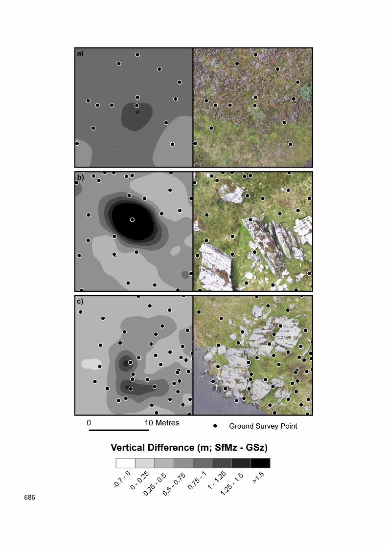
668

Fig. 3 Maps displaying the topographic data and analysis of vertical disagreement. 669

(a) The distribution of 7761 ground-survey points and 19 SfM ground-control points 670

across the survey area. Two zones (Z1 and Z2) of distinct ground cover are 671

delimited. (b) A hillshaded DSM at 0.088 m per pixel resolution derived from the 672

sUAS–SfM survey. (c) A raster surface of vertical difference produced using an 673

ordinary kriging function at a resolution of 2.1 m per pixel. The spatial extent of the 674

spot heights is delimited by the dashed line. 675

676

Fig. 5 The occurrence of vertical difference in association with: (a) vegetation, (b) 677

near vertical and in places partially overhanging bedrock rafts, and (c) positional 678

misregistration close to near vertical slopes 679

680

681

682

683

684

685

686

Table 1 Statistics for the vertical difference between the Cwm Idwal topographic 687

datasets 688

a Mean Difference 689

Area Total Observations (n) RMSE MD a RMSE (<20

o) RMSE (≥20

o)

All 7761 0.517 0.454 0.468 (n = 4527) 0.578 (n = 3234)

East 1988 0.200 0.155 0.169 (n = 1306) 0.247 (n = 682)

West 5773 0.588 0.557 0.544 (n = 3222) 0.639 (n = 2551)

Z1 244 0.796 0.820 0.789 (n = 102) 0.821 (n = 142)

Z2 205 0.362 0.341 0.354 (n = 152) 0.384 (n = 53)

Table 2 Calculated RMSE for vertical difference binned by slope angle. 690

Bin RMSE Observations (n)

0 – 9 0.444 1864

10 – 19 0.482 2662

20 – 29 0.543 1967

30 – 39 0.603 952

40 – 49 0.678 263

50 – 59 0.739 36

60 – 69 0.729 10

70 – 79 0.838 6

80 – 90 2.222 1

691

692

Table 3 Comparative table of known vertical differences between SfM topographic 693

surveys and various validation datasets in a range of geomorphological 694

environments 695

Study Geomorphological setting

Camera Camera Platform

Survey Altitude (m AGL)

Validation Data

Vertical Difference

Westoby et al. (2012)

Coastal SLR: Model not specified

None Ground-level Terrestrial Laser Scanner

94% points values within +/- 1 m

Hugenholtz et al.. (2013)

Aeolian Olympus PEN Mini E-PM1

Fixed-wing sUAS

200 RTK GPS RMSE = 0.29 m

Fonstad et al. (2013)

Exposed Bedrock/Fluvial

Canon A480 Helikite 10-70 LiDAR RMSE = 1.05 m

Javernick et al.. (2014)

Fluvial (Braided Channel)

Canon (10.1 MP): Model not specified.

Full-scale helicopter

600-800 RTK GPS RMSE = 0.13 – 0.37 m

This study Glacial landforms (Vegetated)

Canon EOS-M (18 MP)

Multi-rotor sUAS

117 (average) Total Station

RMSE = East: 0.200 m West: 0.588 m All: 0.517 m

696