http://www.cambridge.org/9780521632010

This page intentionally left blank

Econometric Society Monographs No. 30

Regression analysisof count data

Regression Analysis of Count Data

Students in both the natural and social sciences often seek regressionmodels to explain the frequency of events, such as visits to a doc-tor, auto accidents, or new patents awarded. This analysis provides themost comprehensive and up-to-date account of models and methods tointerpret such data. The authors have conducted research in the field fornearly 15 years and in this work combine theory and practice to makesophisticated methods of analysis accessible to practitioners workingwith widely different types of data and software. The treatment willbe useful to researchers in areas such as applied statistics, economet-rics, marketing, operations research, actuarial studies, demography,biostatistics, and quantitatively oriented sociology and political sci-ence. The book may be used as a reference work on count models orby students seeking an authoritative overview. The analysis is com-plemented by template programs available on the Internet through theauthors’ homepages.

A. Colin Cameron is Associate Professor of Economics at the Uni-versity of California, Davis. He has also taught at the Ohio State Uni-versity and held visiting positions at the Australian National Univer-sity, Indiana University at Bloomington, and the University of NewSouth Wales. His research on count data and microeconometrics hasappeared in many leading econometrics journals.

Pravin K. Trivedi is Professor of Economics at Indiana Univer-sity at Bloomington and previously taught at the Australian NationalUniversity and University of Southampton. He has also held visitingpositions at the European University Institute and the World Bank. Hispublications on count data and micro- and macro-econometrics haveappeared in most leading econometrics journals.

Econometric Society Monographs

Editors:

Peter Hammond, Stanford UniversityAlberto Holly, University of Lausanne

The Econometric Society is an international society for the advancement of eco-nomic theory in relation to statistics and mathematics. The Econometric SocietyMonograph Series is designed to promote the publication of original researchcontributions of high quality in mathematical economics and theoretical andapplied econometrics.

Other titles in the series:

G.S. Maddala Limited-dependent and qualitative variables in econometrics,0 521 33825 5Gerard Debreu Mathematical economics: Twenty papers of Gerard Debreu,0 521 33561 2Jean-Michel Grandmont Money and value: A reconsideration of classicaland neoclassical monetary economics, 0 521 31364 3Franklin M. Fisher Disequilibrium foundations of equilibrium economics,0 521 37856 7Andreu Mas-Colell The theory of general economic equilibrium: Adifferentiable approach, 0 521 26514 2, 0 521 38870 8Cheng Hsiao Analysis of panel data, 0 521 38933 XTruman F. Bewley, Editor Advances in econometrics – Fifth World Congress(Volume I), 0 521 46726 8Truman F. Bewley, Editor Advances in econometrics – Fifth World Congress(Volume II), 0 521 46725 XHerve Moulin Axioms of cooperative decision making, 0 52136055 2,0 521 42458 5L.G. Godfrey Misspecification tests in econometrics: The Lagrangemultiplier principle and other approaches, 0 521 42459 3Tony Lancaster The econometric analysis of transition data, 0 521 43789 XAlvin E. Roth and Marilda A. Oliviera Sotomayor, Editors Two-sidedmatching: A study in game-theoretic modeling and analysis, 0 521 43788 1Wolfgang Hardle Applied nonparametric regression, 0 521 42950 1Jean-Jacques Laffont, Editor Advances in economic theory – Sixth WorldCongress (Volume I), 0 521 48459 6Jean-Jacques Laffont, Editor Advances in economic theory – Sixth WorldCongress (Volume II), 0 521 48460 XHalbert White Estimation, inference and specification analysis,0 521 25280 6, 0 521 57446 3Christopher Sims, Editor Advances in econometrics – Sixth World Congress(Volume I), 0 521 56610 X

(Series list continues on page after index.)

Regression Analysis ofCount Data

A. Colin Cameron

Pravin K. Trivedi

Cambridge, New York, Melbourne, Madrid, Cape Town, Singapore, São Paulo

Cambridge University PressThe Edinburgh Building, Cambridge , United Kingdom

First published in print format

ISBN-13 978-0-521-63201-0 hardback

ISBN-13 978-0-521-63567-7 paperback

ISBN-13 978-0-511-06827-0 eBook (EBL)

© A. Colin Cameron and Pravin K. Trivedi 1998

1998

Information on this title: www.cambridge.org/9780521632010

This book is in copyright. Subject to statutory exception and to the provision ofrelevant collective licensing agreements, no reproduction of any part may take placewithout the written permission of Cambridge University Press.

ISBN-10 0-511-06827-1 eBook (EBL)

ISBN-10 0-521-63201-3 hardback

ISBN-10 0-521-63567-5 paperback

Cambridge University Press has no responsibility for the persistence or accuracy ofs for external or third-party internet websites referred to in this book, and does notguarantee that any content on such websites is, or will remain, accurate or appropriate.

Published in the United States by Cambridge University Press, New York

www.cambridge.org

To Michelle and Bhavna

Contents

List of Figures page xiList of Tables xiiPreface xv

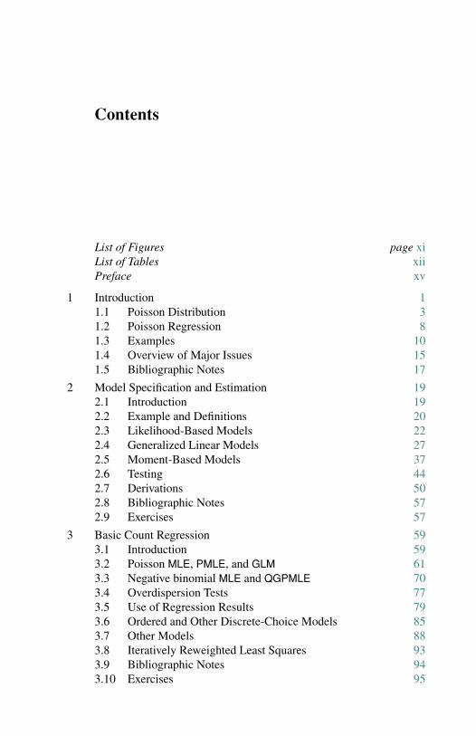
1 Introduction 11.1 Poisson Distribution 31.2 Poisson Regression 81.3 Examples 101.4 Overview of Major Issues 151.5 Bibliographic Notes 17

2 Model Specification and Estimation 192.1 Introduction 192.2 Example and Definitions 202.3 Likelihood-Based Models 222.4 Generalized Linear Models 272.5 Moment-Based Models 372.6 Testing 442.7 Derivations 502.8 Bibliographic Notes 572.9 Exercises 57

3 Basic Count Regression 593.1 Introduction 593.2 Poisson MLE, PMLE, and GLM 613.3 Negative binomial MLE and QGPMLE 703.4 Overdispersion Tests 773.5 Use of Regression Results 793.6 Ordered and Other Discrete-Choice Models 853.7 Other Models 883.8 Iteratively Reweighted Least Squares 933.9 Bibliographic Notes 943.10 Exercises 95

viii Contents

4 Generalized Count Regression 964.1 Introduction 964.2 Mixture Models for Unobserved Heterogeneity 974.3 Models Based on Waiting-Time Distributions 1064.4 Katz, Double-Poisson, and Generalized Poisson 1124.5 Truncated Counts 1174.6 Censored Counts 1214.7 Hurdle and Zero-Inflated Models 1234.8 Finite Mixtures and Latent Class Analysis 1284.9 Estimation by Simulation 1344.10 Derivations 1354.11 Bibliographic Notes 1364.12 Exercises 137

5 Model Evaluation and Testing 1395.1 Introduction 1395.2 Residual Analysis 1405.3 Goodness of Fit 1515.4 Hypothesis Tests 1585.5 Inference with Finite Sample Corrections 1635.6 Conditional Moment Specification Tests 1685.7 Discriminating among Nonnested Models 1825.8 Derivations 1855.9 Bibliographic Notes 1875.10 Exercises 188

6 Empirical Illustrations 1896.1 Introduction 1896.2 Background 1906.3 Analysis of Demand for Health Services 1926.4 Analysis of Recreational Trips 2066.5 LR Test: A Digression 2166.6 Concluding Remarks 2186.7 Bibliographic Notes 2196.8 Exercises 220

7 Time Series Data 2217.1 Introduction 2217.2 Models for Time Series Data 2227.3 Static Regression 2267.4 Integer-Valued ARMA Models 2347.5 Autoregressive Models 2387.6 Serially Correlated Error Models 2407.7 State-Space Models 2427.8 Hidden Markov Models 2447.9 Discrete ARMA Models 2457.10 Application 246

Contents ix

7.11 Derivations: Tests of Serial Correlation 2487.12 Bibliographic Notes 2507.13 Exercises 250

8 Multivariate Data 2518.1 Introduction 2518.2 Characterizing Dependence 2528.3 Parametric Models 2568.4 Moment-Based Estimation 2608.5 Orthogonal Polynomial Series Expansions 2638.6 Mixed Multivariate Models 2698.7 Derivations 2728.8 Bibliographic Notes 273

9 Longitudinal Data 2759.1 Introduction 2759.2 Models for Longitudinal Data 2769.3 Fixed Effects Models 2809.4 Random Effects Models 2879.5 Discussion 2909.6 Specification Tests 2939.7 Dynamic and Transition Models 2949.8 Derivations 2999.9 Bibliographic Notes 3009.10 Exercises 300

10 Measurement Errors 30110.1 Introduction 30110.2 Measurement Errors in Exposure 30210.3 Measurement Errors in Regressors 30710.4 Measurement Errors in Counts 30910.5 Underreported Counts 31310.6 Derivations 32310.7 Bibliographic Notes 32410.8 Exercises 325

11 Nonrandom Samples and Simultaneity 32611.1 Introduction 32611.2 Alternative Sampling Frames 32611.3 Simultaneity 33111.4 Sample Selection 33611.5 Bibliographic Notes 343

12 Flexible Methods for Counts 34412.1 Introduction 34412.2 Efficient Moment-Based Estimation 34512.3 Flexible Distributions Using Series Expansions 35012.4 Flexible Models of Conditional Mean 356

x Contents

12.5 Flexible Models of Conditional Variance 35812.6 Example and Model Comparison 36412.7 Derivations 36712.8 Count Models: Retrospect and Prospect 36712.9 Bibliographic Notes 369

Appendices:

A Notation and Acronyms 371

B Functions, Distributions, and Moments 374B.1 Gamma Function 374B.2 Some Distributions 375B.3 Moments of Truncated Poisson 376

C Software 378

References 379Author Index 399Subject Index 404

List of Figures

1.1 Frequency distribution of counts for four types of events. 114.1 Negative binomial compared with Poisson. 1004.2 Two examples of double Poisson. 1154.3 Two univariate two-component mixtures of Poisson. 1305.1 Comparison of Pearson, deviance, and Anscombe residuals. 1435.2 Takeover bids: residual plots. 1506.1 OFP visits: directional gradients. 2006.2 OFP visits: component densities from the FMNB2 NB1 model. 2037.1 Strikes: output (rescaled) and strikes per month. 2327.2 Strikes: actual and predicted from a static model. 2337.3 Strikes: actual and predicted from a dynamic model. 248

List of Tables

3.1 Doctor visits: actual frequency distribution. 683.2 Doctor visits: variable definitions and summary statistics. 683.3 Doctor visits: Poisson PMLE with different standard error

estimates. 693.4 Doctor visits: NB2 and NB1 model estimators and standard

errors. 763.5 Doctor visits: Poisson PMLE mean effects and scaled

coefficients. 833.6 Doctor visits: alternative estimates and t ratios. 924.1 Doctor visits: GEC(k) and gamma MLE and t ratios. 1145.1 Takeover bids: actual frequency distribution. 1475.2 Takeover bids: variable definitions and summary statistics. 1475.3 Takeover bids: Poisson PMLE with NB1 standard errors and

t ratios. 1485.4 Takeover bids: descriptive statistics for various residuals. 1495.5 Takeover bids: correlations of various residuals. 1495.6 Takeover bids: Poisson MLE predicted and actual

probabilities. 1586.1 OFP visits: actual frequency distribution. 1936.2 OFP visits: variable definitions and summary statistics. 1946.3 OFP visits: likelihood ratio tests. 1996.4 OFP visits: information criteria (AIC and BIC). 2006.5 OFP visits: FMNB2 NB1 model, actual, fitted distributions

and goodness-of-fit tests. 2016.6 OFP visits: FMNB2 NB1 model estimates and standard errors. 2016.7 OFP visits: FMNB2 NB1 model fitted means and variances. 2026.8 OFP visits: NB2 hurdle model estimates and t ratios. 2076.9 Recreational trips: actual frequency distribution. 2086.10 Recreational trips: variable definitions and summary

statistics. 2086.11 Recreational trips: Poisson, NB2, and ZIP model estimates

and t ratios. 209

List of Tables xiii

6.12 Recreational trips: finite mixture estimates and t ratios. 2126.13 Recreational trips: hurdle model estimates and t ratios. 2146.14 Recreational boating trips: actual and fitted cumulative

frequencies. 2156.15 Rejection frequencies at nominal 10% significance level. 2177.1 Strikes: variable definitions and summary statistics. 2317.2 Strikes: Poisson PMLE with NB1 standard errors and t ratios. 2327.3 Strikes: residuals autocorrelations and serial correlation tests. 2337.4 Strikes: Zeger-Qaqish autoregressive model estimates and

diagnostics. 2478.1 Orthogonal polynomials: first and second order. 2698.2 Health services: pairwise independence tests. 2699.1 Patents: Poisson PMLE with NB1 standard errors. 286

12.1 Recreational trips: flexible distribution estimators and tratios. 365

12.2 Recreational trips: cumulative predicted probabilities. 366

Preface

This book describes regression methods for count data, where the responsevariable is a nonnegative integer. The methods are relevant for analysis ofcounts that arise in both social and natural sciences.

Despite their relatively recent origin, count data regression methods buildon an impressive body of statistical research on univariate discrete distribu-tions. Many of these methods have now found their way into major statisticalpackages, which has encouraged their application in a variety of contexts. Suchwidespread use has itself thrown up numerous interesting research issues andthemes, which we explore in this book.

The objective of the book is threefold. First, we wish to provide a synthesisand integrative survey of the literature on count data regressions, covering boththe statistical and econometric strands. The former has emphasized the frame-work of generalized linear models, exponential families of distributions, andgeneralized estimating equations; the latter has emphasized nonlinear regres-sion and generalized method of moment frameworks. Yet between them thereare numerous points of contact that can be fruitfully exploited. Our secondobjective is to make sophisticated methods of data analysis more accessible topractitioners with different interests and backgrounds. To this end we considermodels and methods suitable for cross-section, time series, and longitudinaldata. Detailed analyses of several data sets as well as shorter illustrations, im-plemented from a variety of viewpoints, are scattered throughout the book toput empirical flesh on theoretical or methodological discussion. We draw onexamples from, and give references to, works in many applied areas. Our thirdobjective is to highlight the potential for further research by discussion of is-sues and problems that need more analysis. We do so by embedding count datamodels in a larger body of econometric and statistical work on discrete variablesand, more generally, on nonlinear regression.

The book can be divided into four parts. Chapters 1 and 2 contain introduc-tory material on count data and a comprehensive review of statistical methodsfor nonlinear regression models. Chapters 3, 4, 5, and 6 present models andapplications for cross-section count data. Chapters 7, 8, and 9 present meth-ods for data other than cross-section data, namely time series, multivariate, and

xvi Preface

longitudinal or panel data. Chapters 10, 11, and 12 present methods for commoncomplications, including measurement error, sample selection and simultane-ity, and semiparametric methods. Thus the coverage of the book is qualitativelysimilar to that in a complete single book on linear regression models.

The book is directed toward researchers, graduate students, and other prac-titioners in a wide range of fields. Because of our background in econometrics,the book emphasizes issues arising in econometric applications. Our trainingand background also influence the organizational structure of the book, butareas outside econometrics are also considered. The essential prerequisite forthis book is familiarity with the linear regression model using matrix algebra.The material in the book should be accessible to people with a background inregression and statistical methods up to the level of a standard first-year gradu-ate econometrics text such as Greene’s Econometric Analysis. Although basiccount data methods are included in major statistical packages, more advancedanalysis can require programming in languages such as SPLUS, GAUSS, orMATLAB.

Our own entry into the field of count data models dates back to the early1980s, when we embarked on an empirical study of the demand for health in-surance and health care services at the Australian National University. Sincethen we have been involved in many empirical investigations that have influ-enced our perceptions of this field. We have included numerous data-analyticdiscussions in this volume, to reflect our own interests and those of readersinterested in real data applications. The data sets, computer programs, and re-lated materials used in this book are available through Internet access to thewebsite http://www.econ.ucdavis.edu/count.html. These materials supplementand complement this book and will help new entrants to the field, epeciallygraduate students, to make a relatively easy start.

We have learned much on modeling count data through collaborationswith coauthors, notably Partha Deb, Shiferaw Gurmu, Per Johansson, KajalMukhopadhyay, and Frank Windmeijer. The burden of writing this book hasbeen eased by help from many colleagues, coauthors, and graduate students. Inparticular, we thank the following for their generous attention, encouragement,help, and comments on earlier drafts of various chapters: Kurt Brannas, DavidHendry, Primula Kennedy, Tony Lancaster, Scott Long, Xing Ming, GrayhamMizon, Neil Shephard, and Bob Shumway, in addition to the coauthors alreadymentioned. We especially thank David Hendry and Scott Long for their de-tailed advice on manuscript preparation using Latex software and ScientificWorkplace. The manuscript has also benefited from the comments of a refereeand the series editor, Alberto Holly, and from the guidance of Scott Parris ofCambridge University Press.

Work on the book was facilitated by periods spent at various institutions.The first author thanks the Department of Statistics and the Research School ofSocial Sciences at the Australian National University, the Department of Eco-nomics at Indiana University–Bloomington, and the University of California,Davis, for support during extended leaves at these institutions in 1995 and

Preface xvii

1996. The second author thanks Indiana University and the European UniversityInstitute, Florence, for support during his tenure as Jean Monnet Fellow in 1996,which permitted a period away from regular duties. For shorter periods of staythat allowed us to work jointly, we thank the Department of Economics at Indi-ana University, SELAPO at University of Munich, and the European UniversityInstitute.

Finally we would both like to thank our families for their patience andforbearance, especially during the periods of intensive work on the book. Thiswork would not have been possible at all without their constant support.

A. Colin CameronDavis, California

Pravin K. TrivediBloomington, Indiana

CHAPTER 1

Introduction

God made the integers, all the rest is the work of man.Kronecker

This book is concerned with models of event counts. An event count refersto the number of times an event occurs, for example the number of airlineaccidents or earthquakes. An event count is the realization of a nonnegativeinteger-valued random variable. A univariate statistical model of event countsusually specifies a probability distribution of the number of occurrences of theevent known up to some parameters. Estimation and inference in such modelsare concerned with the unknown parameters, given the probability distributionand the count data. Such a specification involves no other variables and thenumber of events is assumed to be independently identically distributed (iid).Much early theoretical and applied work on event counts was carried out inthe univariate framework. The main focus of this book, however, is regressionanalysis of event counts.

The statistical analysis of counts within the framework of discrete paramet-ric distributions for univariate iid random variables has a long and rich history(Johnson, Kotz, and Kemp, 1992). The Poisson distribution was derived as alimiting case of the binomial by Poisson (1837). Early applications includethe classic study of Bortkiewicz (1898) of the annual number of deaths frombeing kicked by mules in the Prussian army. A standard generalization of thePoisson is the negative binomial distribution. It was derived by Greenwood andYule (1920), as a consequence of apparent contagion due to unobserved het-erogeneity, and by Eggenberger and Polya (1923) as a result of true contagion.The biostatistics literature of the 1930s and 1940s, although predominantlyunivariate, refined and brought to the forefront seminal issues that have sincepermeated regression analysis of both counts and durations. The developmentof the counting process approach unified the treatment of counts and dura-tions. Much of the vast literature on iid counts, which addresses issues suchas heterogeneity and overdispersion, true versus apparent contagion, and iden-tifiability of Poisson mixtures, retains its relevance in the context of count

2 1. Introduction

data regressions. This leads to models such as the negative binomial regressionmodel.

Significant early developments in count models took place in actuarial sci-ence, biostatistics, and demography. In recent years these models have alsobeen used extensively in economics, political science, and sociology. The spe-cial features of data in their respective fields of application have fueled deve-lopments that have enlarged the scope of these models. An important mile-stone in the development of count data regression models was the emergenceof the “generalized linear models,” of which the Poisson regression is a spe-cial case, first described by Nelder and Wedderburn (1972) and detailed inMcCullagh and Nelder (1989). Building on these contributions, the papersby Gourieroux, Monfort, and Trognon (1984a, b), and the work on longitu-dinal or panel count data models of Hausman, Hall, and Griliches (1984),have also been very influential in stimulating applied work in the econometricliterature.

Regression analysis of counts is motivated by the observation that in many,if not most, real-life contexts, the iid assumption is too strong. For example, themean rate of occurrence of an event may vary from case to case and may dependon some observable variables. The investigator’s main interest therefore maylie in the role of covariates (regressors) that are thought to affect the parametersof the conditional distribution of events, given the covariates. This is usuallyaccomplished by a regression model for event count. At the simplest levelwe may think of this in the conventional regression framework in which thedependent variable, y, is restricted to be a nonnegative random variable whoseconditional mean depends on some vector of regressors, x.

At a different level of abstraction, an event may be thought of as the real-ization of a point process governed by some specified rate of occurrence of theevent. The number of events may be characterized as the total number of suchrealizations over some unit of time. The dual of the event count is the inter-arrival time, defined as the length of the period between events. Count dataregression is useful in studying the occurrence rate per unit of time conditionalon some covariates. One could instead study the distribution of interarrivaltimes conditional on covariates. This leads to regression models of waitingtimes or durations. The type of data available, cross-sectional, time series, orlongitudinal, will affect the choice of the statistical framework.

An obvious first question is whether “special” methods are required to handlecount data or whether the standard Gaussian linear regression may suffice. Morecommon regression estimators and models, such as the ordinary least squaresin the linear regression model, ignore the restricted support for the dependentvariable. This leads to significant deficiencies unless the mean of the counts ishigh, in which case normal approximation and related regression methods maybe satisfactory.

The Poisson (log-linear) regression is motivated by the usual considera-tions for regression analysis but also seeks to preserve and exploit as much

1.1. Poisson Distribution 3

as possible the nonnegative and integer-valued aspect of the outcome. At onelevel one might simply regard this as a special type of nonlinear regression thatrespects the discreteness of the count variable. In some analyses this specificdistributional assumption may be given up, while preserving nonnegativity.

In econometrics the interest in count data models is a reflection of the gene-ral interest in modeling discrete aspects of individual economic behavior. Forexample, Pudney (1989) characterizes a large body of microeconometrics as“econometrics of corners, kinks and holes.” Count data models are specific typesof discrete data regressions. Discrete and limited dependent variable modelshave attracted a great deal of attention in econometrics and have found a richset of applications in microeconometrics (Maddala, 1983), especially as econo-metricians have attempted to develop models for the many alternative types ofsample data and sampling frames. Although the Poisson regression provides astarting point for many analyses, attempts to accommodate numerous real-lifeconditions governing observation and data collection lead to additional elabo-rations and complications.

The scope of count data models is very wide. This monograph addressesissues that arise in the regression models for counts, with a particular focus onfeatures of economic data. In many cases, however, the material covered canbe easily adapted for use in social and natural sciences, which do not alwaysshare the peculiarities of economic data.

1.1 Poisson Distribution

The benchmark model for count data is the Poisson distribution. It is useful atthe outset to review some fundamental properties and characterization resultsof the Poisson distribution (for derivations see Taylor and Karlin, 1994).

If the discrete random variable Y is Poisson-distributed with intensity or rateparameter µ, µ > 0, and t is the exposure, defined as the length of time duringwhich the events are recorded, then Y has density

Pr[Y = y] = e−µt (µt)y

y!, y = 0, 1, 2, . . . (1.1)

where E[Y ] = V[Y ] = µt . If we set the length of the exposure period t equalto unity, then

Pr[Y = y] = e−µµy

y!, y = 0, 1, 2, . . . (1.2)

This distribution has a single parameter µ, and we refer to it as P[µ]. Its kth

raw moment, E[Y k], may be derived by differentiating the moment generatingfunction (mgf) k times

M(t) ≡ E[etY ] = expµ(et − 1),

4 1. Introduction

with respect to t and evaluating at t = 0. This yields the following four rawmoments:

µ′1 = µ

µ′2 = µ + µ2

µ′3 = µ + 3µ2 + µ3

µ′4 = µ + 7µ2 + 6µ3 + µ4.

Following convention, raw moments are denoted by primes, and central mo-ments without primes. The central moments around µ can be derived from theraw moments in the standard way. Note that the first two central moments,denoted µ1 and µ2, respectively, are equal to µ. The central moments satisfythe recurrence relation

µr+1 = rµµr−1 + µ∂µr

∂µ, r = 1, 2, . . . . (1.3)

where µ0 = 0.Equality of the mean and variance will be referred to as the equidispersion

property of the Poisson. This property is frequently violated in real-life data.Overdispersion (underdispersion) means the variance exceeds (is less than) themean.

A key property of the Poisson distribution is additivity. This is stated by thefollowing countable additivity theorem (for a mathematically precise statementsee Kingman, 1993).

Theorem. If Yi ∼ P[µi ], i = 1, 2, . . . are independent random variables, and if∑µi < ∞, then SY =∑ Yi ∼ P[

∑µi ].

The binomial and the multinomial can be derived from the Poisson by ap-propriate conditioning. Under the conditions stated,

Pr [Y1 = y1, Y2 = y2, . . . , Yn = yn | SY = s]

=[

n∏j=1

e−µ j µy j

j

y j !

]/[(∑µi)s

e−∑µi

s!

]

= s!

y1!y2! . . . yn!

(µ1∑µi

)y1(

µ2∑µi

)y2

. . .

(µn∑

µi

)yn

.

= s!

y1!y2! . . . yn!π

y11 π

y22 . . . π yn

n , (1.4)

where π j = µ j/∑

µi . This is the multinomial distribution m[s; π1, . . . , πn].The binomial is the case n = 2.

There are many characterizations of the Poisson distribution. Here we con-sider four. The first, the law of rare events, is a common motivation for the

1.1. Poisson Distribution 5

Poisson. The second, the Poisson counting process, is very commonly encoun-tered in introduction to stochastic processes. The third is simply the dual ofthe second, with waiting times between events replacing the count. The fourthcharacterization, Poisson-stopped binomial, treats the number of events as rep-etitions of a binomial outcome, with the number of repetitions taken as Poissondistributed.

1.1.1 Poisson as the “Law of Rare Events”

The law of rare events states that the total number of events will follow, ap-proximately, the Poisson distribution if an event may occur in any of a largenumber of trials but the probability of occurrence in any given trial is small.

More formally, let Yn,π denote the total number of successes in a largenumber n of independent Bernoulli trials with success probability π of eachtrial being small. Then

Pr[Yn,π = k] =(

n

k

)π k(1 − π )n−k, k = 0, 1, . . . , n.

In the limiting case where n → ∞, π → 0, and nπ = µ > 0, that is, theaverage µ is held constant while n → ∞, we have

limn→∞

[(n

k

)(µ

n

)k(1 − µ

n

)n−k]= µke−µ

k!,

the Poisson probability distribution with parameter µ, denoted as P[µ].

1.1.2 Poisson Process

The Poisson distribution has been described as characterizing “complete ran-domness” (Kingman, 1993). To elaborate this feature the connection betweenthe Poisson distribution and the Poisson process needs to be made explicit. Suchan exposition begins with the definition of a counting process.

A stochastic process N (t), t ≥ 0 is defined to be a counting process ifN (t) denotes an event count up to time t . N (t) is nonnegative and integer-valued and must satisfy the property that N (s) ≤ N (t) if s < t , and N (t) − N (s)is the number of events in the interval (s, t]. If the event counts in disjoint timeintervals are independent, the counting process is said to have independentincrements. It is said to be stationary if the distribution of the number of eventsdepends only on the length of the interval.

The Poisson process can be represented in one dimension as a set of pointson the time axis representing a random series of events occurring at points oftime. The Poisson process is based on notions of independence and the Poissondistribution in the following sense.

Define µ to be the constant rate of occurrence of the event of interest, andN (s, s + h), to be the number of occurrence of the event in the time interval

6 1. Introduction

(s, s + h]. A (pure) Poisson process of rate µ occurs if events occur indepen-dently with constant probability equal to µ times the length of the interval. Thenumbers of events in disjoint time intervals are independent, and the distribu-tion of events in each interval of unit length is P[µ]. Formally, as the length ofthe interval h → 0,

Pr[N (s, s + h) = 0] = 1 − µh + o(h)

Pr[N (s, s + h) = 1] = µh + o(h),(1.5)

where o(h) denotes a remainder term with the property o(h)/h → 0 as h → 0.N (s, s + h) is statistically independent of the number and position of events in(s, s + h]. Note that in the limit the probability of two or more events occurringis zero; 0 and 1 events occur with probabilities of, respectively, (1−µh) and µh.For this process it can be shown (Taylor and Karlin, 1994) that the number ofevents occurring in the interval (s, s + h], for nonlimit h, is Poisson distributedwith mean µh and probability

Pr[N (s, s + h) = r ] = e−µh(µh)r

r !r = 0, 1, 2, . . . (1.6)

Normalizing the length of the exposure time interval to be unity, h = 1, leadsto the Poisson density given previously. In summary, the counting process N (t)with stationary and independent increments and N (0) = 0, which satisfies (1.5),generates events that follow the Poisson distribution.

1.1.3 Waiting Time Distributions

We now consider a characterization of the Poisson that is the flip side of thatgiven in the immediately preceding paragraph. Let W1 denote the time of thefirst event, and Wr , r ≥ 1, the time between the (r − 1)th and r th event. Thenonnegative random sequence Wr , r ≥ 1 is called the sequence of interarrivaltimes, waiting times, durations, or sojourn times. In addition to, or instead of,analyzing the number of events occurring in the interval of length h, one cananalyze the duration of time between successive occurrences of the event, orthe time of occurrence of the r th event, Wr . This requires the distribution of Wr ,which can be determined by exploiting the duality between event counts andwaiting times. This is easily done for the Poisson process.

The outcome W1 > t occurs only if no events occur in the interval (0, t].That is,

Pr[W1 > t] = Pr[N (t) = 0] = e−µt , (1.7)

which implies that W1 has exponential distribution with mean 1/µ. The waitingtime to the first event, W1, is exponentially distributed with density fW1 (t) =µe−µt , t ≥ 0. Also,

Pr[W2 > t |W1 = s] = Pr[N (s, s + t) = 0 | W1 = s]

= Pr[N (s, s + t) = 0]

= e−µt ,

1.1. Poisson Distribution 7

using the properties of independent stationary increments. This argument canbe repeated for Wr to yield the result that Wr , r = 1, 2, . . . , are iid exponentialrandom variables with mean 1/µ. This result reflects the property that thePoisson process has no memory.

In principle, the duality between number of occurrences and time betweenoccurrences suggests that count and duration data should be covered in the sameframework. Consider the arrival time of the r th event, denoted Sr ,

Sr =r∑

i=1

Wi , r ≥ 1. (1.8)

It can be shown using results on sums of random variables that Sr has gammadistribution

fSr (t) = µr tr−1

(r − 1)!e−µt , t ≥ 0. (1.9)

The above result can also be derived by observing that

N (t) ≥ r ⇔ Sr ≤ t. (1.10)

Hence

Pr[N (t) ≥ r ] = Pr[Sr ≤ t]

=∞∑j=r

e−µt (µt) j

j!. (1.11)

To obtain the density of Sr , the cumulative density function (cdf) given above isdifferentiated with respect to t . Thus, the Poisson process may be characterizedin terms of the implied properties of the waiting times.

Suppose one’s main interest is in the role of the covariates that determinethe Poisson process rate parameter µ. For example, let µ = exp(x′β). Hence,the mean waiting time is given by 1/µ = exp(−x′β), confirming the intuitionthat the covariates affect the mean number of events and the waiting times inopposite directions. This illustrates that from the viewpoint of studying therole of covariates, analyzing the frequency of events is the dual complement ofanalyzing the waiting times between events.

The Poisson process is often too restrictive in practice. Mathematicallytractable and computationally feasible common links between more generalcount and duration models are hard to find (see Chapter 4).

In the waiting time literature, emphasis is on estimating the hazard rate, theconditional instantaneous probability of the event occurring given that it has notyet occurred, controlling for censoring due to not always observing occurrenceof the event. Fleming and Harrington (1991) and Andersen, Borgan, Gill, andKeiding (1993) present, in great detail, models for censored duration data basedon application of martingale theory to counting processes.

We focus on counts. Even if duration is the more natural entity for analysis,it may not be observed. If only event counts are available, count regressions

8 1. Introduction

still provide an opportunity for studying the role of covariates in explaining themean rate of event occurrence. However, count analysis leads in general to aloss of efficiency (Dean and Balshaw, 1997).

1.1.4 Binomial Stopped by the Poisson

Yet another characterization of the Poisson involves mixtures of the Poissonand the binomial. Let n be the actual (or true) count process taking nonnegativeinteger values with E[n] = µ, and V[n] = σ 2. Let B1, B2, . . . , Bn be a sequenceof n independent and identically distributed Bernoulli trials, in which each B j

takes one of only two values, 1 or 0, with probabilities π and 1−π , respectively.Define the count variable Y = ∑n

i=1 Bi . For n given, Y follows a binomialdistribution with parameters n and π . Hence,

E[Y ] = E[E[Y | n]] = E[nπ ] = πE[n] = µπ

V[Y ] = V[E[Y | n]] + E[V[Y | n]] = (σ 2 − µ)π2 + µπ.(1.12)

The actual distribution of Y depends on the distribution of n. For Poisson-distributed n it can be found using the following lemma.

Lemma. If π is the probability that Bi = 1, i = 1, . . . , n, and 1 − π the proba-bility that Bi = 0, and n ∼ P[µ], then Y ∼ P[µπ ].

To derive this result begin with the probability generating function (pgf),defined as g(s) = E[s B], of the Bernoulli random variable

g(s) = (1 − π ) + πs, (1.13)

for any real s. Let f (s) denote the pgf of the Poisson variable n, E[sn], that is,

f (s) = exp(−µ + µs). (1.14)

Then the pgf of Y is obtained as

f (g(s)) = exp[−µ + µg(s)]

= exp[−µπ + µπs], (1.15)

which is the pgf of Poisson-distributed Y with parameter µπ . This charac-terization of the Poisson has been called the Poisson-stopped binomial. Thischaracterization is useful if the count is generated by a random number ofrepetitions of a binary outcome.

1.2 Poisson Regression

The approach taken to the analysis of count data, especially the choice of theregression framework, sometimes depends on how the counts are assumed toarise. There are two common formulations. In the first, they arise from a directobservation of a point process. In the second, counts arise from discretization(“ordinalization”) of continuous latent data. Other less-used formulations ap-peal, for example, to the law of rare events or the binomial stopped by Poisson.

1.2. Poisson Regression 9

1.2.1 Counts Derived from a Point Process

Directly observed counts arise in many situations. Examples are the number oftelephone calls arriving at a central telephone exchange, the number of monthlyabsences at the place of work, the number of airline accidents, the number ofhospital admissions, and so forth. The data may also consist of interarrivaltimes for events. In the simplest case, the underlying process is assumed tobe stationary and homogeneous, with iid arrival times for events and otherproperties stated in the previous section.

1.2.2 Counts Derived from Continuous Data

Count-type variables sometimes arise from categorization of a latent continu-ous variable as the following example indicates. Credit rating of agencies maybe stated as “AAA,” “AAB,” “AA,” “A,” “BBB,” “B,” and so forth, where“AAA” indicates the greatest credit worthiness. Suppose we code these asy = 0, 1, . . . , m. These are pseudocounts that can be analyzed using a countregression. But one may also regard this as an ordinal ranking that can be mod-eled using a suitable latent variable model such as ordered probit. Chapter 3provides a more detailed exposition.

1.2.3 Regression Specification

The standard model for count data is the Poisson regression model, which is anonlinear regression model. This regression model is derived from the Poissondistribution by allowing the intensity parameter µ to depend on covariates(regressors). If the dependence is parametrically exact and involves exogenouscovariates but no other source of stochastic variation, we obtain the standardPoisson regression. If the function relating µ and the covariates is stochastic,possibly because it involves unobserved random variables, then one obtains amixed Poisson regression, the precise form of which depends on the assumptionsabout the random term. Chapter 4 deals with several examples of this type.

A standard application of Poisson regression is to cross-section data. Typi-cal cross-section data for applied work consist of n independent observations,the i th of which is (yi , xi ). The scalar dependent variable, yi , is the number ofoccurrences of the event of interest, and xi is the vector of linearly independentregressors that are thought to determine yi . A regression model based on thisdistribution follows by conditioning the distribution of yi on a k-dimensionalvector of covariates, x′

i = [x1i , . . . , xki ], and parameters β, through a continu-ous function µ(xi ,β), such that E[yi | xi ] = µ(xi ,β).

That is, yi given xi is Poisson-distributed with density

f (yi | xi ) = e−µi µyi

i

yi !, yi = 0, 1, 2, . . . (1.16)

In the log-linear version of the model the mean parameter is parameterized as

µi = exp(x′

iβ), (1.17)

10 1. Introduction

to ensure µ > 0. Equations (1.16) and (1.17) jointly define the Poisson (log-linear) regression model. If one does not wish to impose any distributionalassumptions, the Eq. (1.17) by itself may be used for (nonlinear) regressionanalysis.

For notational economy we write f (yi | xi ) in place of the more formalf (Yi = yi | xi ), which distinguishes between the random variable Y and its re-alization y. By the property of the Poisson, V[yi | xi ] = E[yi | xi ], implyingthat the conditional variance is not a constant, and hence the regression is in-trinsically heteroskedastic. In the log-linear version of the model the meanparameter is parameterized as (1.17), which implies that the conditional meanhas a multiplicative form given by

E[yi | xi ] = exp(x′

iβ)

= exp(x1iβ1) exp(x2iβ2) · · · exp(xkiβk),

with interest often lying in changes in this conditional mean due to changesin the regressors. The additive specification, E[yi | xi ] = x′

iβ = ∑kj=1 x jiβi ,

is likely to be unsatisfactory because certain combinations of βi and xi willviolate the nonnegativity restriction on µi .

The Poisson model is closely related to the models for analyzing counted datain the form of proportions or ratios of counts sometimes obtained by groupingdata. In some situations, for example when the population “at risk” is changingover time in a known way, it is helpful to reparameterize the model as follows.Let y be the observed number of events (e.g., accidents), N the known totalexposure to risk (i.e., number “at risk”), and x the known set of k explanatoryvariables. The mean number of events µ may be expressed as the product ofN and π , the probability of the occurrence of event, sometimes also called thehazard rate. That is, µ(x) = N (x)π (x,β). In this case the probability π isparameterized in terms of covariates. For example, π = exp(x′β). This leadsto a rate form of the Poisson model with the density

Pr[Y = y | N (x), x] = e−µ(x)µ(x)y

y!, y = 0, 1, 2, . . . (1.18)

Variants of the Poisson regression arise in a number of ways. As was men-tioned previously, the presence of an unobserved random error term in the con-ditional mean function, denoted νi , implies that we specify it as E[yi | xi , νi ].The marginal distribution of yi will involve the moments of the distribution ofνi . This is one way in which mixed Poisson distributions may arise.

1.3 Examples

Patil (1970) gives numerous applications of count data analysis in the sciences.This earlier work is usually not in the regression context. There are now manyexamples of count data regression models in statistics and econometrics whichuse cross-sectional, time series or longitudinal data. For example, models ofcounts of doctor visits and other types of health care utilization; occupational

1.3. Examples 11

injuries and illnesses; absenteeism in the workplace; recreational or shoppingtrips; automobile insurance rate making; labor mobility; entry and exits fromindustry; takeover activity in business; mortgage prepayments and loan defaults;bank failures; patent registration in connection with industrial research anddevelopment; and frequency of airline accidents. There are many applicationsalso in demographic economics, in crime victimology, in marketing, politicalscience and government, sociology and so forth. Many of the earlier applicationsare univariate treatments, not regression analyses.

The data used in many of these applications have certain commonalities.Events considered are often rare. The “law of rare events” is famously exem-plified by Bortkiewicz’s 1898 study of the number of soldiers kicked to deathin Prussian stables. Zero event counts are often dominant, leading to a skeweddistribution. Also, there may be a great deal of unobserved heterogeneity inthe individual experiences of the event in question. Unobserved heterogeneityleads to overdispersion; that is, the actual variance of the process exceeds thenominal Poisson variance even after regressors are introduced.

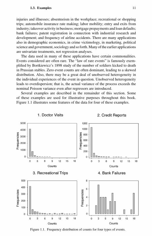
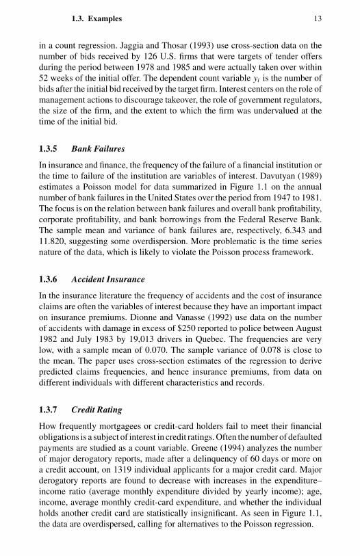
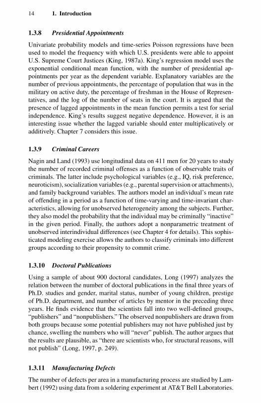
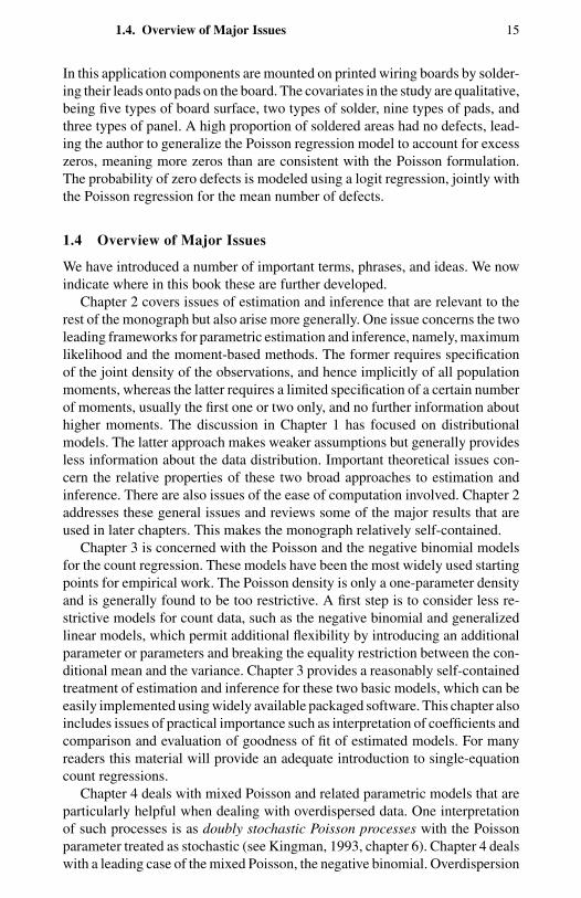
Several examples are described in the remainder of this section. Someof these examples are used for illustrative purposes throughout this book.Figure 1.1 illustrates some features of the data for four of these examples.

Figure 1.1. Frequency distribution of counts for four types of events.

12 1. Introduction

1.3.1 Health Services

Health economics research is often concerned with the link between health-service utilization and economic variables such as income and price, especiallythe latter, which can be lowered considerably by holding a health insurancepolicy. Ideally one would measure utilization by expenditures, but if data comefrom surveys of individuals it is more common to have data on the number oftimes that health services are consumed, such as the number of visits to a doctorin the past month and the number of days in hospital in the past year, becauseindividuals can better answer such questions than those on expenditure.

Data sets with healthcare utilization measured in counts include the NationalHealth Interview Surveys and the Surveys on Income and Program Participationin the United States, the German Socioeconomic Panel (Wagner, Burkhauser,and Behringer, 1993), and the Australian Health Surveys (Australian Bureauof Statistics, 1978). Data on the number of doctor consultations in the past 2weeks from the 1977–78 Australian Health Survey (see Figure 1.1) are analyzedusing cross-section Poisson and negative binomial models by Cameron andTrivedi (1986) and Cameron, Trivedi, Milne, and Piggott (1988). Figure 1.1highlights overdispersion in the form of excess zeros.

1.3.2 Patents

The link between research and development and product innovation is an im-portant issue in empirical industrial organization. Product innovation is difficultto measure, but the number of patents is one indicator of it. This measure iscommonly analyzed. Panel data on the number of patents received annually byfirms in the United States are analyzed by Hausman, Hall, and Griliches (1984)and in many subsequent studies.

1.3.3 Recreational Demand

In environmental economics one is often interested in alternative uses of a nat-ural resource such as forest or parkland. To analyze the valuation placed onsuch a resource by recreational users, economists often model the frequencyof the visits to particular sites as a function of the cost of usage and the eco-nomic and demographic characteristics of the users. For example, Ozuna andGomaz (1995) analyze 1980 survey data on the number of recreational boatingtrips to Lake Somerville in East Texas. Again, Figure 1.1 displays overdisper-sion and excess zeros.

1.3.4 Takeover Bids

In empirical finance the bidding process in a takeover is sometimes studiedeither using the probability of any additional takeover bids, after the first, usinga binary outcome model, or using the number of bids as a dependent variable

1.3. Examples 13

in a count regression. Jaggia and Thosar (1993) use cross-section data on thenumber of bids received by 126 U.S. firms that were targets of tender offersduring the period between 1978 and 1985 and were actually taken over within52 weeks of the initial offer. The dependent count variable yi is the number ofbids after the initial bid received by the target firm. Interest centers on the role ofmanagement actions to discourage takeover, the role of government regulators,the size of the firm, and the extent to which the firm was undervalued at thetime of the initial bid.

1.3.5 Bank Failures

In insurance and finance, the frequency of the failure of a financial institution orthe time to failure of the institution are variables of interest. Davutyan (1989)estimates a Poisson model for data summarized in Figure 1.1 on the annualnumber of bank failures in the United States over the period from 1947 to 1981.The focus is on the relation between bank failures and overall bank profitability,corporate profitability, and bank borrowings from the Federal Reserve Bank.The sample mean and variance of bank failures are, respectively, 6.343 and11.820, suggesting some overdispersion. More problematic is the time seriesnature of the data, which is likely to violate the Poisson process framework.

1.3.6 Accident Insurance

In the insurance literature the frequency of accidents and the cost of insuranceclaims are often the variables of interest because they have an important impacton insurance premiums. Dionne and Vanasse (1992) use data on the numberof accidents with damage in excess of $250 reported to police between August1982 and July 1983 by 19,013 drivers in Quebec. The frequencies are verylow, with a sample mean of 0.070. The sample variance of 0.078 is close tothe mean. The paper uses cross-section estimates of the regression to derivepredicted claims frequencies, and hence insurance premiums, from data ondifferent individuals with different characteristics and records.

1.3.7 Credit Rating

How frequently mortgagees or credit-card holders fail to meet their financialobligations is a subject of interest in credit ratings. Often the number of defaultedpayments are studied as a count variable. Greene (1994) analyzes the numberof major derogatory reports, made after a delinquency of 60 days or more ona credit account, on 1319 individual applicants for a major credit card. Majorderogatory reports are found to decrease with increases in the expenditure–income ratio (average monthly expenditure divided by yearly income); age,income, average monthly credit-card expenditure, and whether the individualholds another credit card are statistically insignificant. As seen in Figure 1.1,the data are overdispersed, calling for alternatives to the Poisson regression.

14 1. Introduction

1.3.8 Presidential Appointments

Univariate probability models and time-series Poisson regressions have beenused to model the frequency with which U.S. presidents were able to appointU.S. Supreme Court Justices (King, 1987a). King’s regression model uses theexponential conditional mean function, with the number of presidential ap-pointments per year as the dependent variable. Explanatory variables are thenumber of previous appointments, the percentage of population that was in themilitary on active duty, the percentage of freshman in the House of Represen-tatives, and the log of the number of seats in the court. It is argued that thepresence of lagged appointments in the mean function permits a test for serialindependence. King’s results suggest negative dependence. However, it is aninteresting issue whether the lagged variable should enter multiplicatively oradditively. Chapter 7 considers this issue.

1.3.9 Criminal Careers

Nagin and Land (1993) use longitudinal data on 411 men for 20 years to studythe number of recorded criminal offenses as a function of observable traits ofcriminals. The latter include psychological variables (e.g., IQ, risk preference,neuroticism), socialization variables (e.g., parental supervision or attachments),and family background variables. The authors model an individual’s mean rateof offending in a period as a function of time-varying and time-invariant char-acteristics, allowing for unobserved heterogeneity among the subjects. Further,they also model the probability that the individual may be criminally “inactive”in the given period. Finally, the authors adopt a nonparametric treatment ofunobserved interindividual differences (see Chapter 4 for details). This sophis-ticated modeling exercise allows the authors to classify criminals into differentgroups according to their propensity to commit crime.

1.3.10 Doctoral Publications

Using a sample of about 900 doctoral candidates, Long (1997) analyzes therelation between the number of doctoral publications in the final three years ofPh.D. studies and gender, marital status, number of young children, prestigeof Ph.D. department, and number of articles by mentor in the preceding threeyears. He finds evidence that the scientists fall into two well-defined groups,“publishers” and “nonpublishers.” The observed nonpublishers are drawn fromboth groups because some potential publishers may not have published just bychance, swelling the numbers who will “never” publish. The author argues thatthe results are plausible, as “there are scientists who, for structural reasons, willnot publish” (Long, 1997, p. 249).

1.3.11 Manufacturing Defects

The number of defects per area in a manufacturing process are studied by Lam-bert (1992) using data from a soldering experiment at AT&T Bell Laboratories.

1.4. Overview of Major Issues 15

In this application components are mounted on printed wiring boards by solder-ing their leads onto pads on the board. The covariates in the study are qualitative,being five types of board surface, two types of solder, nine types of pads, andthree types of panel. A high proportion of soldered areas had no defects, lead-ing the author to generalize the Poisson regression model to account for excesszeros, meaning more zeros than are consistent with the Poisson formulation.The probability of zero defects is modeled using a logit regression, jointly withthe Poisson regression for the mean number of defects.

1.4 Overview of Major Issues

We have introduced a number of important terms, phrases, and ideas. We nowindicate where in this book these are further developed.

Chapter 2 covers issues of estimation and inference that are relevant to therest of the monograph but also arise more generally. One issue concerns the twoleading frameworks for parametric estimation and inference, namely, maximumlikelihood and the moment-based methods. The former requires specificationof the joint density of the observations, and hence implicitly of all populationmoments, whereas the latter requires a limited specification of a certain numberof moments, usually the first one or two only, and no further information abouthigher moments. The discussion in Chapter 1 has focused on distributionalmodels. The latter approach makes weaker assumptions but generally providesless information about the data distribution. Important theoretical issues con-cern the relative properties of these two broad approaches to estimation andinference. There are also issues of the ease of computation involved. Chapter 2addresses these general issues and reviews some of the major results that areused in later chapters. This makes the monograph relatively self-contained.

Chapter 3 is concerned with the Poisson and the negative binomial modelsfor the count regression. These models have been the most widely used startingpoints for empirical work. The Poisson density is only a one-parameter densityand is generally found to be too restrictive. A first step is to consider less re-strictive models for count data, such as the negative binomial and generalizedlinear models, which permit additional flexibility by introducing an additionalparameter or parameters and breaking the equality restriction between the con-ditional mean and the variance. Chapter 3 provides a reasonably self-containedtreatment of estimation and inference for these two basic models, which can beeasily implemented using widely available packaged software. This chapter alsoincludes issues of practical importance such as interpretation of coefficients andcomparison and evaluation of goodness of fit of estimated models. For manyreaders this material will provide an adequate introduction to single-equationcount regressions.

Chapter 4 deals with mixed Poisson and related parametric models that areparticularly helpful when dealing with overdispersed data. One interpretationof such processes is as doubly stochastic Poisson processes with the Poissonparameter treated as stochastic (see Kingman, 1993, chapter 6). Chapter 4 dealswith a leading case of the mixed Poisson, the negative binomial. Overdispersion

16 1. Introduction

is closely related to the presence of unobserved interindividual heterogeneity,but it can also arise from occurrence dependence between events. Using cross-section data it may be practically impossible to identify the underlying source ofoverdispersion. These issues are tackled in Chapter 4, which deals with models,especially overdispersed models, that are motivated by “non-Poisson” featuresof data that can occur separately or jointly with overdispersion, for example,an excess of zero observations relative to either the Poisson or the negativebinomial, or the presence of censoring or truncation.

Chapter 5 deals with statistical inference and model evaluation for single-equation count regressions estimated using the methods of earlier chapters. Theobjective is to provide the user with specification tests and model evaluationprocedures that are useful in empirical work based on cross-section data. As inChapter 2, the issues considered in this chapter have relevance beyond count-data models.

Chapter 6 provides detailed analyses of two empirical examples to illus-trate the single-equation modeling approaches of earlier chapters and espe-cially the interplay of estimation and model evaluation that dominates empiricalmodeling.

Chapter 7 deals with time series analysis of event counts. A time series countregression is relevant if data are T observations, the t th of which is (yt , xt ),t = 1, . . . , T . If xt includes past values of yt , we refer to it as a dynamic countregression. This involves modeling the serial correlation in the count process.The static time series count regression as well as dynamic regression modelsare studied. This topic is still relatively underdeveloped.

Multivariate count models are considered in Chapter 8. An m-dimensionalmultivariate count model is based on data on (yi , xi ) where yi is an (m × 1)vector of variables that may all be counts or may include counts as well as otherdiscrete or continuous variables. Unlike the familiar case of the multivariateGaussian distribution, the term multivariate in the case of count models coversa number of different definitions. Hence, Chapter 8 deals more with a numberof special cases and provides relatively few results of general applicability.

Another class of multivariate models uses longitudinal or panel data, whichare analyzed in Chapter 9. Longitudinal count models have attracted muchattention in recent work, following the earlier work of Hausman, Hall, andGriliches (1984). Such models are relevant if the regression analysis is basedon (yit, xit), i = 1, . . . , n; t = 1, . . . , T, where i and t are individual and timesubscripts, respectively. Dynamic panel data models also include lagged y vari-ables. Unobserved random terms may also appear in multivariate and paneldata models. The usefulness of longitudinal data is that without such datait is extremely difficult to distinguish between true contagion and apparentcontagion.

Chapters 10 through 12 contain material based on more recent develop-ments and areas of current research activity. Some of these issues are activelyunder investigation; their inclusion is motivated by our desire to inform the

1.5. Bibliographic Notes 17

reader about the state of the literature and to stimulate further effort. Chapter 10deals with the effects of measurement errors in either exposure or covariates,and with the problem of underrecorded counts. Chapter 11 deals with modelswith simultaneity and nonrandom sampling, including sample selection. Suchmodels are usually estimated with nonlinear instrumental variable estimators.

In the final chapter, Chapter 12, we review several flexible modeling ap-proaches to count data, some of which are based on series expansion methods.These methods permit considerable flexibility in the variance–mean relation-ships and in the estimation of probability of events. Some of them might alsobe described as “semiparametric.”

We have attempted to structure this monograph keeping in mind the inter-ests of researchers, practitioners, and new entrants to the field. The last groupmay wish to gain a relatively quick understanding of the standard models andmethods; practitioners may be interested in the robustness and practicality ofmethods; and researchers wishing to contribute to the field presumably want anup-to-date and detailed account of the different models and methods. Whereverpossible we have included illustrations based on real data. Inevitably, in placeswe have compromised, keeping in mind the constraints on the length of themonograph. We hope that the bibliographic notes and exercises at the ends ofchapters will provide useful complementary material for all users.

In cross-referencing sections we use the convention that, for example, section3.4 refers to section 4 in Chapter 3.

Appendix A lists the acronyms that are used in the book. Some basic mathe-matical functions and distributions and their properties are summarized inAppendix B. Appendix C provides some software information.

Vectors are defined as column vectors, with transposition giving a row vector,and are printed in bold lowercase. Matrices are printed in bold uppercase.

1.5 Bibliographic Notes

Johnson, Kotz, and Kemp (1992) is an excellent reference for statistical prop-erties of the univariate Poisson and related models. A lucid introduction toPoisson processes is in earlier sections of Kingman (1993). A good introduc-tory textbook treatment of Poisson processes and renewal theory is Taylor andKarlin (1994). A more advanced treatment is in Feller (1971). Another compre-hensive reference on Poisson and related distributions with full bibliographicdetails until 1967 is Haight (1967). Early applications of the Poisson regres-sion include Cochran (1940) and Jorgenson (1961). Count data analysis in thesciences is surveyed in a comprehensive three-volume collective work editedby Patil (1970). Although volume 1 is theoretical, the remaining two volumescover many applications in the natural sciences.

There are a number of surveys for count data models; for example, Cameronand Trivedi (1986), Gurmu and Trivedi (1994), and Winkelmann and Zimmer-mann (1995). In both biostatistics and econometrics, and especially in health,

18 1. Introduction

labor, and environmental economics, there are many applications of count mod-els, which are mentioned throughout this book and especially in Chapter 6.Examples of applications in criminology, sociology, political science, and in-ternational relations are Grogger (1990), Nagin and Land (1993), Hannan andFreeman (1987), and King (1987a, b). Examples of application in finance areDionne, Artis and Guillen (1996) and Schwartz and Torous (1993).

CHAPTER 2

Model Specification and Estimation

2.1 Introduction

The general modeling approaches most often used in count data analysis –likelihood-based, generalized linear models, and moment-based – are presentedin this chapter. Statistical inference for these nonlinear regression models isbased on asymptotic theory, which is also summarized.

The models and results vary according to the strength of the distributionalassumptions made. Likelihood-based models and the associated maximum like-lihood estimator require complete specification of the distribution. Statisticalinference is usually performed under the assumption that the distribution iscorrectly specified.

A less parametric analysis assumes that some aspects of the distribution ofthe dependent variable are correctly specified while others are not specified,or if specified are potentially misspecified. For count data models considerableemphasis has been placed on analysis based on the assumption of correct speci-fication of the conditional mean, or on the assumption of correct specification ofboth the conditional mean and the conditional variance. This is a nonlinear gen-eralization of the linear regression model, where consistency requires correctspecification of the mean and efficient estimation requires correct specificationof the mean and variance. It is a special case of the class of generalized linearmodels, widely used in the statistics literature. Estimators for generalized linearmodels coincide with maximum likelihood estimators if the specified densityis in the linear exponential family. But even then the analytical distribution ofthe same estimator can differ across the two approaches if different second mo-ment assumptions are made. The term pseudo- (or quasi-) maximum likelihoodestimation is used to describe the situation in which the assumption of correctspecification of the density is relaxed. Here the first moment of the specifiedlinear exponential family density is assumed to be correctly specified, while thesecond and other moments are permitted to be incorrectly specified.

An even more general framework, which permits estimation based on anyspecified moment conditions, is that of moment-based models. In the statisticsliterature this approach is known as estimating equations. In the econometrics

20 2. Model Specification and Estimation

literature this approach leads to generalized method of moments estimation,which is particularly useful if regressors are not exogenous.

Results for hypothesis testing also depend on the strength of the distribu-tional assumptions. The classical statistical tests – Wald, likelihood ratio, andLagrange multiplier (or score) – are based on the likelihood approach. Ana-logues of these hypothesis tests exist for the generalized method of momentsapproach. Finally, the moments approach introduces a new class of tests ofmodel specification, not just of parameter restrictions, called conditional mo-ment tests.

Section 2.2 presents the simplest count model and estimator, the maximumlikelihood estimator of the Poisson regression model. Notation used throughoutthe book is also explained. The three main approaches – maximum likelihood,generalized linear models, and moment-based models – and associated esti-mation theory are presented in, respectively, sections 2.3 through 2.5. Testingusing these approaches is summarized in section 2.6. Throughout, statisticalinference based on first-order asymptotic theory is given, with results derivedin section 2.7. Small sample refinements such as the bootstrap are deferred tolater chapters.

Basic count data analysis uses maximum likelihood extensively, and alsogeneralized linear models. For more complicated data situations presented inthe latter half of the book, generalized linear models and moment-based modelsare increasingly used.

This chapter is a self-contained source, to be referred to as needed in readinglater chapters. It is also intended to provide a bridge between the statistics andeconometrics literatures. The presentation is of necessity relatively condensedand may be challenging to read in isolation, although motivation for results isgiven. A background at the level of Greene (1997a) or Johnston and DiNardo(1997) is assumed.

2.2 Example and Definitions

2.2.1 Example

The starting point for cross-section count data analysis is the Poisson regressionmodel. This assumes that yi , given the vector of regressors xi , is independentlyPoisson distributed with density

f (yi | xi ) = e−µi µyi

i

yi !, yi = 0, 1, 2, . . . , (2.1)

and mean parameter

µi = exp(x′

iβ), (2.2)

where β is a k × 1 parameter vector. Counting process theory provides a mo-tivation for choosing the Poisson distribution; taking the exponential of x′

iβ in

2.2. Example and Definitions 21

(2.2) ensures that the parameter µi is nonnegative. This model implies that theconditional mean is given by

E[yi | xi ] = exp(x′

iβ), (2.3)

with interest often lying in changes in this conditional mean due to changesin the regressors. It also implies a particular form of heteroskedasticity, due toequidispersion or equality of conditional variance and conditional mean,

V[yi | xi ] = exp(x′

iβ). (2.4)

The standard estimator for this model is the maximum likelihood estimator(MLE). Given independent observations, the log-likelihood function is

L(β) =n∑

i=1

yi x′

iβ − exp(x′

iβ)− ln yi !

. (2.5)

Differentiating (2.5) with respect to β yields the Poisson MLE β as the solutionto the first-order conditions

n∑i=1

(yi − exp

(x′

iβ))

xi = 0. (2.6)

These k equations are nonlinear in the k unknowns β, and there is no analyticalsolution for β. Iterative methods, usually gradient methods such as Newton-Raphson, are needed to compute β. Such methods are given in standard texts.

Another consequence of there being no analytical solution for β is thatexact distributional results for β are difficult to obtain. Inference is accordinglybased on asymptotic results, presented in the remainder of this chapter. Thereare several ways to proceed. First, we can view β as the estimator maximizing(2.5) and apply maximum likelihood theory. Second, we can view β as beingdefined by (2.6). These equations have similar interpretation to those for theordinary least squares (OLS) estimator. That is, the unweighted residual (yi −µi )is orthogonal to the regressors. It is therefore possible that, as for OLS, inferencecan be performed under assumptions about just the mean and possibly variance.This is the generalized linear models approach. Third, because (2.3) impliesE[(yi − exp(x′

iβ))xi ] = 0, we can define an estimator that is the solution to thecorresponding moment condition in the sample, that is, the solution to (2.6).This is the moment-based models approach.

2.2.2 Definitions

We use the generic notation θ ∈ Rq to denote the q × 1 parameter vector tobe estimated. In the Poisson regression example the only parameters are theregression parameters, so θ=β and q = k. In the simplest extensions an ad-ditional scalar dispersion parameter α is introduced, so θ′ = (β′α)′ and q =k + 1.

22 2. Model Specification and Estimation

We consider random variables θ that converge in probability to a value θ∗,

θp→ θ∗,

or equivalently the probability limit (plim) of θ equals θ∗,

plim θ = θ∗.

The probability limit θ∗ is called the pseudotrue value. If the data generatingprocess (dgp) is a model with θ = θ0, and the pseudotrue value actually equalsθ0, so θ0 = θ∗, then θ is said to be consistent for θ0.

Estimators θ used are usually root-n consistent for θ∗ and asymptoticallynormally distributed. Then the random variable

√n(θ − θ∗) converges in dis-

tribution to the multivariate normal distribution with mean 0 and variance C,

√n(θ − θ∗)

d→ N[0, C], (2.7)

where C is a finite positive definite matrix. It is sometimes notationally conve-nient to express (2.7) in the simpler form

θa∼ N[θ∗, D], (2.8)

where D = 1n C. That is, θ is asymptotically normal distributed with mean θ∗

and variance D = 1n C. The division of the finite matrix C by the sample size

makes it clear that as the sample size goes to infinity the variance matrix 1n C

goes to zero, which is to be expected because θp→ θ∗.

The variance matrix C may depend on unknown parameters, and the result(2.8) is operationalized by replacing C by a consistent estimator C. In manycases C = A−1BA′−1, where A and B are finite positive definite matrices. ThenC = A−1BA′−1, where A and B are consistent estimators of A and B. Thisis called the sandwich form, because B is sandwiched between A−1 and A−1

transposed. A more detailed discussion is given in section 2.5.1.Results are expressed using matrix calculus. In general the derivative ∂g(θ)/

∂θ of a scalar function g(θ) with respect to the q × 1 vector θ is a q × 1 vectorwith j th entry ∂g(θ)/∂θ j . The derivative ∂h(θ)/∂θ′ of a r × 1 vector functionh(θ) with respect to the 1 × q vector θ′ is an r × q matrix with jkth entry∂h j (θ)/∂θk .

2.3 Likelihood-Based Models

Likelihood-based models are models in which the joint density of the depen-dent variables is specified. For completeness a review is presented here, alongwith results for the less standard case of maximum likelihood with the densityfunction misspecified.

We assume that the scalar random variable yi , given the vector of regressors xi

and parameter vector θ, is distributed with density f (yi | xi ,θ). The likelihood

2.3. Likelihood-Based Models 23

principle chooses as estimator ofθ the value that maximizes the joint probabilityof observing the sample values y1, . . . , yn . This probability, viewed as a functionof parameters conditional on the data, is called the likelihood function and isdenoted

L(θ) =n∏

i=1

f (yi | xi ,θ), (2.9)

where we suppress the dependence of L(θ) on the data and have assumedindependence over i . This definition implicitly assumes cross-section data butcan easily accommodate time series data by extending xi to include laggeddependent and independent variables.

Maximizing the likelihood function is equivalent to maximizing the log-likelihood function

L(θ) = ln L(θ) =n∑

i=1

ln f (yi | xi ,θ). (2.10)

In the following analysis we consider the local maximum, which we assume toalso be the global maximum.

2.3.1 Regularity Conditions

The standard results on consistency and asymptotic normality of the MLE holdif the so-called regularity conditions are satisfied. Furthermore, the MLE thenhas the desirable property that it attains the Cramer-Rao lower bound and isfully efficient. The following regularity conditions, given in Crowder (1976),are used in many studies.

1. The pdf f (y, x,θ) is globally identified and f (y, x,θ(1)) = f (y, x,

θ(2)), for all θ(1) =θ(2).2. θ ∈ Θ, where Θ is finite dimensional, closed, and compact.3. Continuous and bounded derivatives of L(θ) exist up to order three.4. The order of differentiation and integration of the likelihood may be

reversed.5. The regressor vector xi satisfies

(a) x′i xi < ∞

(b) E[w2i ]∑

i E[w2i ]

= 0 for all i , where wi ≡ x′i∂ ln f (yi | xi ,θ)

∂θ

(c) limn→∞∑n

i=1 E[w2i |i−1]∑n

i=1 E[w2i ]

= 1 where i−1 = (x1, x2, . . . , xi−1).

The first condition is an obvious identification condition, which ensuresthat the limit of 1

nL has a unique maximum. The second condition rules outpossible problems at the boundary of Θ and can be relaxed if, for example, Lis globally concave. The third condition can often be relaxed to existence upto second order. The fourth condition is a key condition that rules out densities

24 2. Model Specification and Estimation

for which the range of yi depends on θ. The final condition rules out anyobservation making too large a contribution to the likelihood. For further detailson regularity conditions for commonly used estimators, not just the MLE, seeNewey and McFadden (1994).

2.3.2 Maximum Likelihood

We consider only the case in which the limit of 1nL is maximized at an interior

point of Θ. The MLE θML is then the solution to the first-order conditions

∂L∂θ

=n∑

i=1

∂ ln fi

∂θ= 0, (2.11)

where fi = f (yi | xi ,θ) and ∂L/∂θ is a q × 1 vector.The asymptotic distribution of the MLE is usually obtained under the assump-

tion that the density is correctly specified. That is, the dgp for yi has densityf (yi | xi ,θ0), where θ0 is the true parameter value. Then, under the regularityconditions, θ

p→ θ0, so the MLE is consistent for θ0. Also,

√n(θML − θ0)

d→ N[0, A−1], (2.12)

where the q × q matrix A is defined as

A = − limn→∞

1

nE

[n∑

i=1

∂2 ln fi

∂θ∂θ′

∣∣∣∣∣θ0

]. (2.13)

A consequence of regularity conditions three and four is the informationmatrix equality

E[

∂2L∂θ∂θ′

]= −E

[∂L∂θ

∂L∂θ′

], (2.14)

for all values of θ ∈ Θ. This is derived in section 2.7. Assuming independenceover i and defining

B = limn→∞

1

nE

[n∑

i=1

∂ ln fi

∂θ

∂ ln fi

∂θ′

∣∣∣∣∣θ0

], (2.15)

the information equality implies A = B.To operationalize these results one needs a consistent estimator of the vari-

ance matrix in Eq. (2.12). There are many possibilities. The (expected) Fisherinformation estimator takes the expectation in (2.13) under the assumed den-sity and evaluates at θ. The Hessian estimator simply evaluates (2.13) at θwithout taking the expectation. The outer-product estimator evaluates (2.15)at θ without taking the expectation. It was proposed by Berndt, Hall, Hall, andHausman (1974) and is also called the BHHH estimator. A more general form

2.3. Likelihood-Based Models 25

of the variance matrix of θML, the sandwich form, is used if the assumption ofcorrect specification of the density is relaxed (see section 2.3.4).

As an example, consider the MLE for the Poisson regression model presentedin section 2.1. In this case ∂L/∂β =∑i (yi − exp(x′

iβ))xi and

∂2L/∂β∂β′ = −∑

i

exp(x′

iβ)xi x′

i .

It follows that we do not even need to take the expectation in (2.13) to obtain

A = limn→∞

1

n

[∑i

exp(x′

iβ0)xi x′

i

].

Assuming E[(yi −exp(x′iβ0))2|xi ] = exp(x′

iβ0), that is, correct specification ofthe variance, leads to the same expression for B. The result is most convenientlyexpressed as

βMLa∼ N

(β0,

(n∑

i=1

exp(x′

iβ0)xi x′

i

)−1). (2.16)

In this case the Fisher information and Hessian estimators of V[θML] coincide,and differ from the outer-product estimator.

2.3.3 Profile Likelihood

Suppose the likelihood depends on a parameter vector λ in addition to θ, so thelikelihood function isL(θ,λ). The profile likelihood or concentrated likelihoodeliminates λ by obtaining the restricted MLE λ(θ) for fixed θ. Then

Lpro(θ) = L(θ, λ(θ)). (2.17)

This approach can be used in all situations, but it is important to note thatLpro(θ) is not strictly a log-likelihood function and that the usual results needto be adjusted in this case (see, for example, Davidson and MacKinnon, 1993,chapter 8).

The profile likelihood is useful if λ is a nuisance parameter. For example,interest may lie in modeling the conditional mean parameterized by θ, withvariance parametersλ not intrinsically of interest. In such circumstances there isadvantage to attempting to estimateθ alone, especially ifλ is of high dimension.

For scalar θ the profile likelihood can be used to form a likelihood ratio100(1 − α)% confidence region for θ , θ : Lpro(θ ) > L(θ , λ) − χ2

1 (α), whereL(θ , λ) is the unconstrained maximum likelihood. This need not be symmetricaround θ , unlike the usual confidence interval θ ± zα/2se[θ ], where se[θ ] is thestandard error of θ .

Other variants of the likelihood approach can be used to eliminate nuisanceparameters in some special circumstances. The conditional likelihood is the

26 2. Model Specification and Estimation

joint density of θ conditional on a sufficient statistic for the nuisance parametersand is used, for example, to estimate the fixed effects Poisson model for paneldata. The marginal likelihood is the likelihood for a subset of the data that maydepend on θ alone. For further discussion see McCullagh and Nelder (1989,chapter 7).

2.3.4 Misspecified Density

A weakness of the ML approach is that it assumes correct specification of thecomplete density. To see the role of this assumption, it is helpful to begin with aninformal proof of consistency of the MLE in the usual case of correctly specifieddensity.

The MLE solves the sample moment condition ∂L/∂θ= 0, so an intuitivenecessary condition for consistency is that the same moment condition holds inthe population or E[∂L/∂θ] = 0, which holds if E[∂ ln fi/∂θ] = 0. Any densityf (y | x,θ) satisfying the regularity conditions has the property that∫

∂ ln f (y |θ)

∂θf (y |θ) dy = 0; (2.18)

see section 2.7 for a derivation. The consistency condition E[∂ ln f (y | x,θ)/∂θ] = 0 is implied by (2.18), if the expectations operator is taken using theassumed density f (y | x,θ).

Suppose instead that the dgp is the density f ∗(yi | zi ,γ) rather than theassumed density f (yi | xi ,θ). Then, Eq. (2.18) no longer implies the consistencycondition E[∂ ln f (y | x,θ)/∂θ] = 0, which now becomes∫

∂ ln f (y | x,θ)

∂θf ∗(y | z,γ) dy = 0,

as the expectation should be with respect to the dgp density, not the assumeddensity. Thus, misspecification of the density may lead to inconsistency.

White (1982), following Huber (1967), obtained the distribution of the MLEif the density function is incorrectly specified. In general θML

p→ θ∗, where thepseudotrue valueθ∗ is the value ofθ that maximizes plim 1

n

∑ni=1 ln f (yi | xi ,θ)

and the probability limit is obtained under the dgp f ∗(yi | zi ,γ). Under suitableassumptions,

√n(θML − θ∗)

d→ N[0, A−1

∗ B∗A−1∗], (2.19)

where

A∗ = − limn→∞

1

nE∗

[n∑

i=1

∂2 ln fi

∂θ∂θ′

∣∣∣∣∣θ∗

](2.20)

2.4. Generalized Linear Models 27

and

B∗ = limn→∞

1

nE∗

[n∑

i=1

∂ ln fi

∂θ

∂ ln fi

∂θ′

∣∣∣∣∣θ∗

], (2.21)

where fi = f (yi | xi ,θ) and the expectations E∗ are with respect to the dgpf ∗(yi | zi ,γ).

The essential point is that if the density is misspecified the ML estimator is ingeneral inconsistent. Generalized linear models, presented next, are the notableexception. A second point is that the MLE has the more complicated variancefunction with the sandwich form (2.19), because the information matrix equality(2.14) no longer holds. The sandwich estimator of the variance matrix of θML

is A−1BA−1. Different estimates of A and B can be used (see section 2.3.2)depending on whether or not the expectations in A∗ and B∗ are taken beforeevaluation at θML. The robust sandwich estimator does not take expectations.

2.4 Generalized Linear Models

Although the MLE is in general inconsistent if the density is incorrectly spec-ified, for some specified densities consistency may be maintained even givenpartial misspecification of the model. A leading example is maximum likeli-hood estimation in the linear regression model under the assumption that yi

is independently N[x′iβ0, σ

2] distributed. Then βML equals the OLS estimator,which may be consistent even given nonnormality and heteroskedasticity, asthe essential requirement for consistency is correct specification of the condi-tional mean: E[yi | xi ] = x′

iβ0. A similar situation arises for the Poisson regres-sion model. Consistency essentially requires that the population analogue ofEq. (2.6) holds:

E[(yi − exp

(x′

iβ0))

xi ] = 0.

This is satisfied, however, if E[yi | xi ] = exp(x′iβ0). More generally such re-

sults hold for maximum likelihood estimation of models with specified densitya member of the linear exponential family, and estimation of the closely relatedclass of generalized linear models.

Although consistency in these models requires only correct specificationof the mean, misspecification of the variance leads to invalid statistical infer-ence due to incorrect reported t-statistics and standard errors. For example,in the linear regression model the usual reported standard errors for OLS areincorrect if the error is heteroskedastic rather than homoskedastic. Adjustmentto the usual computer output needs to be made to ensure correct standard er-rors. Furthermore, more efficient generalized least squares (GLS) estimation ispossible.

We begin with a presentation of results for weighted least squares for linearmodels, results that carry over to generalized linear models. We then introducegeneralized linear models by considering linear exponential family models.

28 2. Model Specification and Estimation

These models are based on a one-parameter distribution, which in practice istoo restrictive. Extensions to two-parameter models have been made in twoways – the linear exponential family with nuisance parameter and generalizedlinear models. Further results for generalized linear models are then presentedbefore concluding with extended generalized linear models.

2.4.1 Weighted Linear Least Squares

Consider the linear regression model for yi with nonstochastic regressors xi .In the linear model the regression function is x′

iβ0. Suppose it is believedthat heteroskedasticity exists and as a starting point can be approximated byV[yi ] = vi where vi is known. Then one uses the weighted least squares (WLS)estimator with weights 1/vi , which solves the first-order conditions

n∑i=1

1

vi

(yi − x′

iβ)xi = 0. (2.22)

We consider the distribution of this estimator if the mean is correctly specifiedbut the variance is not necessarily vi . It is helpful to express the first-orderconditions in matrix notation as

X′V−1(y − Xβ) = 0, (2.23)

where y is the n × 1 vector with i th entry yi , X is the n × k matrix with i th

row x′i , and V is the n × n weighting matrix with i th diagonal entry vi . These

equations have the analytical solution

βWLS = (X′V−1X)−1X′V−1y.

To obtain the mean and variance of βWLS we assume y has mean Xβ0 andvariance matrix Ω. Then it is a standard result that E[βWLS] = β0 and

V[βWLS] = (X′V−1X)−1X′V−1ΩV−1X(X′V−1X)−1. (2.24)

One familiar example of this is OLS. Then V = σ 2I and V[βWLS] = (X′X)−1

X′ΩX(X′X)−1, which simplifies to σ 2(X′X)−1 if Ω= σ 2I. A second familiarexample is GLS, with V =Ω, in which case V[βWLS] = (X′Ω−1X)−1.

It is important to note that the general result (2.24) represents a differentsituation to that in standard textbook treatments. One begins with a workinghypothesis about the form of the heteroskedasticity, say vi , leading to a workingvariance matrix V. If V is misspecified then βWLS is still unbiased, but it isinefficient and most importantly has a variance matrix of the general form(2.24), which does not impose V =Ω. One way to estimate V[βWLS] is tospecify Ω to be a particular function of regressors and parameters and obtainconsistent estimates of these parameters and hence a consistent estimator Ω ofΩ. Alternatively, White (1980) (see also Eicker, 1967) gave conditions underwhich one need not specify the functional form for the variance matrix Ω but

2.4. Generalized Linear Models 29

can instead use the matrix Ω= Diag[(yi − x′i βWLS)2], where Diag[ai ] denotes

the diagonal matrix with i th diagonal entry ai . The justification is that eventhough Ω is not consistent for Ω, the difference between the k × k matrices1n X′V−1ΩV−1X and 1

n X′V−1ΩV−1X has probability limit zero.These same points carry over to generalized linear models. One specifies a

working variance assumption such as variance–mean equality for the Poisson.The dependence of vi on µi does not change the result (2.24). Hence failure ofthis assumption does not lead to inconsistency if the mean is correctly specifiedbut will lead to incorrect inference if one does not use the general form (2.24).Generalized linear models have an additional complication, because the meanfunction is nonlinear. This can be accommodated by generalizing the first-orderconditions (2.22). Because in the linear case µi = x′

iβ, (2.22) can be reexpressedas

n∑i=1

1

vi(yi − µi )

∂µi

∂β= 0. (2.25)

The first-order conditions for generalized linear models such as the Poisson areof the form (2.25). It can be shown that the discussion above still holds, withthe important change that the matrix X in (2.23) and (2.24) is now defined tohave i th row ∂µi/∂β

′.There is considerable overlap in the next three subsections, which cover

different representations and variations of essentially the same model. In sec-tions 2.4.2 and 2.4.3 the density is parameterized in terms of the mean parameter;in section 2.4.4 the density is parameterized in terms of the so-called canonicalparameter. The latter formulation is used in the generalized linear models liter-ature. To those unfamiliar with this literature the mean parameter formulationmay be more natural. For completeness both presentations are given here. Othervariations, such as different ways nuisance scale parameters are introduced, arediscussed at the end of section 2.4.4.

2.4.2 Linear Exponential Family Models

The presentation follows Cameron and Trivedi (1986), whose work was basedon Gourieroux, Monfort, and Trognon (1984a). A density fLEF(y | µ) is a mem-ber of a linear exponential family (LEF) with mean parameterization if

fLEF(y | µ) = expa(µ) + b(y) + c(µ)y, (2.26)

where µ = E[y], and the functions a(·) and c(·) are such that

E[y] = −[c′(µ)]−1a′(µ), (2.27)

where a′(µ) = ∂a(µ)/∂µ and c′(µ) = ∂c(µ)/∂µ, and

V[y] = [c′(µ)]−1. (2.28)

30 2. Model Specification and Estimation

The function b(·) is a normalizing constant. Different functional forms for a(·)and c(·) lead to different LEF models. Special cases of the LEF include thenormal (with σ 2 known), Poisson, geometric, binomial (with number of trialsfixed), exponential, and one-parameter gamma.

For example, the Poisson density can be written as exp−µ+ y ln µ− ln y!,which is an LEF model with a(µ) = −µ, c(µ) = ln µ and b(y) = − ln y! Thena′(µ) = −1 and c′(µ) = 1/µ, so E[y] = µ from Eq. (2.27) and V[y] = µ from(2.28).

Members of the exponential family have density f (y | λ) = expa(λ) +b(y) + c(λ)t(y). The LEF is the special case t(y) = y, hence the qualifier linear.The natural exponential family has density f (y | λ) = expa(λ) + λy. Otherexponential families come from the natural exponential family by one-to-onetransformations x = t(y) of y.

A regression model is formed by specifying the density to be fLEF(yi | µi )where

µi = µ(xi ,β), (2.29)

for some specified mean function µ(·). The MLE based on an LEF, βLEF,maximizes

LLEF =n∑

i=1

a(µi ) + b(yi ) + c(µi )yi . (2.30)

The first-order conditions using Eqs. (2.27) and (2.28) can be rewritten as

n∑i=1

1

vi(yi − µi )

∂µi

∂β= 0, (2.31)

where

vi = [c′(µi )]−1 (2.32)

is the specified variance function which is a function of µi and hence β. Thesefirst-order conditions are of the form (2.25), and as seen subsequently we obtainresults similar to (2.24).

It is helpful at times to rewrite (2.31) as

n∑i=1

(yi − µi )√vi

1√vi

∂µi

∂β= 0, (2.33)

which shows that the standardized residual is orthogonal to the standardizedregressor.

Under the standard assumption that the density is correctly specified, so thedgp is fLEF(yi | µ(xi ,β0)), application of (2.12) and (2.13) yields

√n(βLEF − β0)

d→ N[0, A−1], (2.34)

2.4. Generalized Linear Models 31

where

A = limn→∞

1

n

n∑i=1

1

vi

∂µi

∂β

∂µi

∂β′

∣∣∣∣β0

. (2.35)

Now consider estimation if the density is misspecified. Gourieroux et al.(1984a) call the estimator in this case the pseudomaximum likelihood (PML)estimator. Other authors call such an estimator a quasimaximum likelihoodestimator. Throughout this book we use the term PML to avoid confusion withthe conceptually different quasilikelihood introduced in section 2.4.5.

Assume (yi , xi ) is independent over i , the conditional mean of yi is correctlyspecified as E[yi | xi ] = µ(xi ,β0), and

V[yi | xi ] = ωi (2.36)

is finite, but ωi = vi necessarily. Thus the mean is correctly specified but otherfeatures of the distribution such as the variance and density are potentially mis-specified. Then Gourieroux et al. (1984a) show that βLEF

p→ β0, so the MLEis still consistent for β0. The intuition is that consistency of βLEF essentiallyrequires that

E[

1

vi(yi − µi )

∂µi

∂β

∣∣∣∣β0

]= 0,

so that the conditions (2.31) hold in the population. This is the case if theconditional mean is correctly specified because then E[yi − µ(xi ,β0) | xi ] = 0.

Also√

n(βLEF − β0)d→ N[0, A−1BA−1], (2.37)

where A is defined in Eq. (2.35) and

B = limn→∞

1

n

n∑i=1

ωi

v2i

∂µi

∂β

∂µi

∂β′

∣∣∣∣β0

. (2.38)

Note that vi is the working variance, the variance in the specified LEF densityfor yi , while ωi is the variance for the true dgp. Note also that (2.37) equals(2.24) where X is the n × k matrix with i th row ∂µi/∂β

′, V = diag[vi ] andΩ= diag[ωi ], confirming the link with results for weighted linear least squares.

There are three important results. First, regardless of other properties ofthe true dgp for y, the PML estimator based on an assumed LEF is consistentprovided the conditional mean is correctly specified. This result is sometimesmisinterpreted. It should be clear that it is the assumed density that must beLEF, while the true dgp need not be LEF.

Second, correct specification of the mean and variance is sufficient for theusual maximum likelihood output to give the correct variance matrix for the PMLestimator based on an assumed LEF density. Other moments of the distributionmay be misspecified.

32 2. Model Specification and Estimation

Third, if the only part of the model that is correctly specified is the condi-tional mean, the MLE is consistent, but the usual maximum likelihood outputgives an inconsistent estimate of the variance matrix, because it uses A−1 ratherthan the sandwich form A−1BA−1. This is correct only if B = A, which re-quires ωi = vi , that is, correct specification of the conditional variance of thedependent variable.

Correct standard errors are obtained by using as variance matrix 1n A−1BA−1

where A and B equal A and B defined in, respectively, (2.35) and (2.37), eval-uated at µi = µ(xi , βLEF), v2

i = [c′(µi )]−1 and ωi . The estimate of the truevariance ωi can be obtained in two ways. First, if no assumptions are madeabout the variance one can use ωi = (yi − µi )2 by extension of results for theOLS estimator given by White (1980). Even though ωi does not converge toωi , under suitable assumptions B

p→ B. Secondly, a structural model for thevariance can be specified, say as ωi = ω(xi ,β,α), where α is a finite dimen-sional nuisance parameter. Then we can use ωi = ω(xi , βLEF, α) where α is aconsistent estimate of α. Particularly convenient is ωi = αvi , as then B = αAso that A−1BA−1 = αA−1.

As an example, consider the Poisson regression model with exponentialmean function µi = exp(x′

iβ). Then ∂µi/∂β= µi xi . The Poisson specifies thevariance to equal the mean, so vi = ωi . Substituting in (2.35) yields

A = lim1

n

∑i

µi xi x′i ,

and similarly (2.38) yields

B = lim1

n

∑i

ωi xi x′i .

In general for correctly specified conditional mean the Poisson PML estimator isasymptotically normal with mean β0 and variance 1

n A−1BA−1. If additionallyωi = vi = µi so that the conditional variance of yi is correctly specified, thenA = B and the variance of the estimator simplifies to 1

n A−1.

2.4.3 LEF with Nuisance Parameter

Given specification of a true variance function, so ωi = ω(·), one can potentiallyobtain a more efficient estimator, in the same way that specification of thefunctional form of heteroskedasticity in the linear regression model leads to themore efficient GLS estimator.

Gourieroux et al. (1984a) introduced the more general variance function

ωi = ω(µ(xi ,β), α) (2.39)

by defining the LEF with nuisance parameter (LEFN)

fLEFN(y | µ, α) = expa(µ, α) + b(y, α) + c(µ, α)y, (2.40)

2.4. Generalized Linear Models 33

whereµ = E[y],ω(µ, α) = V[y], andα = ψ(µ, ω) whereψ(·) is a differentiablefunction of α and ω and ψ(·) defines for any given µ a one-to-one relationshipbetween α and ω. For given α this is an LEF density, so the functions a(·) andc(·) satisfy (2.27) and (2.28), with c(µ, α) and a(µ, α) replacing c(µ) and a(µ).

Gourieroux et al. (1984a) proposed the quasigeneralized pseudomaximumlikelihood (QGPML) estimator βLEFN based on LEFN, which maximizes withrespect to β

LLEFN =n∑

i=1

a(µi , ω(µi , α)) + b(yi , ω(µi , α)) + c(µi , ω(µi , α))yi (2.41)

where µi = µ(xi , β) and β and α are root-n consistent estimates of β and α.The first-order conditions can be reexpressed as

n∑i=1

1

ωi(yi − µi )

∂µi

∂β= 0. (2.42)

Assume (yi , xi ) is independent over i , and the conditional mean and varianceof yi are correctly specified, so E[yi | xi ] = µ(xi ,β0) and V[yi | xi ] = ω(µ(xi ,

β0), α0). Then βLEFNp→ β0, so the QGPML estimator is consistent forβ0. Also

√n(βLEFN − β0)

d→ N[0, A−1], (2.43)

where

A = limn→∞

1

n

n∑i=1

1

ωi

∂µi

∂β

∂µi

∂β′

∣∣∣∣β0

. (2.44)

A consistent estimate for the variance matrix is obtained by evaluating A atµi = µ(xi , βLEFN) and ωi = ω(µi , α). One can, of course, guard against possiblemisspecification of ωi in the same way that possible misspecification of vi washandled in the previous subsection.

The negative binomial model with mean µ and variance µ+αµ2 is an exam-ple of an LEFN model. The QGPMLE of this model is considered in section 3.3.

2.4.4 Generalized Linear Models

Generalized linear models (GLMs), introduced by Nelder and Wedderburn(1972), are closely related to the LEFN model. Differences include a notationalone due to use of an alternative parameterization of the exponential family, andseveral simplifications including the use of more restrictive parameterizations ofthe conditional mean and variance than (2.29) and (2.39). A very useful simplesummary of GLMs is presented in McCullagh and Nelder (1989, chapter 2).

34 2. Model Specification and Estimation

A density fGLM(y | θ, φ) is a member of a linear exponential family withcanonical (or natural) parameter θ and nuisance parameter φ if

fGLM(y | θ, φ) = exp

θy − b(θ )

a(φ)+ c(y, φ)

. (2.45)

The function b(·) is such that

E[y] = b′(θ ), (2.46)

where b′(θ) = ∂b(θ )/∂θ . The function a(φ) is such that

V[y] = a(φ)b′′(θ ), (2.47)

where b′′(θ ) = ∂2b(θ )/∂θ2. Usually a(φ) = φ. The function c(·) is a normalizingconstant. Different functional forms for a(·) and b(·) lead to different GLMs.Note that the functions a(·), b(·), and c(·) for the GLM are different from thefunctions a(·), b(·), and c(·) for the LEF and LEFN.

As an example, the Poisson is the case b(θ ) = exp(θ ), a(φ) = 1, and c(y, φ) =ln y!. Then (2.46) and (2.47) yield E[y] = V[y] = exp(θ ).

Regressors are introduced in the following way. Define the linear predictor

η = x′β. (2.48)

The link function η = η(µ) relates the linear predictor to the mean µ. For ex-ample, the Poisson model with mean µ = exp(x′β) corresponds to the log linkfunction η = ln µ. A special case of the link function of particular interest isthe canonical link function, when

η = θ. (2.49)

For the Poisson the log link function is the canonical link function, becauseb(θ ) = exp(θ ) implies µ = b′(θ ) = exp(θ ), so η = ln µ = ln(exp(θ )) = θ .

The concept of link function can cause confusion. It is more natural toconsider the inverse of the link function, which is the conditional mean function.Thus, for example, the log link function is best thought of as being an exponentialconditional mean function. The canonical link function is most easily thoughtof as leading to the density (2.45) being evaluated at θ = x′β.

The MLE based on a GLM, βGLM, maximizes

LGLM =n∑

i=1

θ(x′

iβ)yi − b

(θ(x′

iβ))

a(φ) + c(yi , φ

). (2.50)

The first-order conditions can be reexpressed as

n∑i=1

1

ωi(yi − µi )

∂µi

∂β= 0, (2.51)

2.4. Generalized Linear Models 35

where the variance function

ωi = a(φ)υ(µ(x′

iβ))

, (2.52)

and

υ(µi ) = b′′(θi ). (2.53)

The first-order conditions (2.51) for the GLM are of similar form to thefirst-order conditions (2.42) for the LEFN. This is because these two modelsare essentially the same. To link the two models, invert µ = b′(θ ) to obtainθ = d(µ). Then (2.45) can be rewritten as

fGLM(y | µ, φ) = exp

−b(d(µ))

a(φ)+ c(y, φ) + d(µ)

a(φ)y

, (2.54)

which is clearly of the form (2.40), with the restriction that in (2.45) a(µ, φ) = a1

(µ)/a2(φ) and c(µ, φ) = c1(µ)/c2(φ). This simplification implies that the GLMvariance function ω(µ(x′

iβ), φ) is multiplicative in φ, so that the first-orderconditions can be solved for β without knowledge of φ. This is not necessarilya trivial simplification. For example, for Poisson with a nuisance parameter theGLM model specifies the variance function to be of multiplicative form a(φ)µ.The LEFN model allows, however, variance functions such as the quadraticform µ + φµ2.

The same asymptotic theory as in section 2.4.3 therefore holds. Assume(yi , xi ) is independent over i , and the conditional mean and variance of yi arecorrectly specified, so E[yi | xi ] = µ(xi ,β0) and V(yi | xi ) = a(φ0)υ(µ(xi ,β0)).Then βGLM

p→ β0, so the MLE is consistent for β0. Also

√n(βGLM − β0)

d→ N[0, A−1] (2.55)

where

A = limn→∞

1

n

n∑i=1

1

ωi

∂µi

∂β

∂µi

∂β′

∣∣∣∣β0

. (2.56)

A consistent estimate of the variance matrix is obtained by evaluating A atµi = µ(xi , βGLM) and ωi = a(φ)υ(µi ). The standard estimate of φ is obtainedfrom

a(φ) = 1

n − k

n∑i=1

(yi − µi )2

υ(µi ). (2.57)

Usually a(φ) = φ.In summary, the basic GLM model is based on the same density as the LEF

and LEFN models presented in sections 2.4.2 through 2.4.3. It uses a differentparameterization of the LEF, canonical and not mean, that is less natural ifinterest lies in modeling the conditional mean. The only real difference in the

36 2. Model Specification and Estimation

models is that the basic GLM model of Nelder and Wedderburn (1972) imposessome simplifying restrictions on the LEFN model that Gourieroux et al. (1984a)consider.

First, the conditional mean function µ(xi ,β) is restricted to be a function ofa linear combination of the regressors and so is of the simpler form µ(x′

iβ). Thisspecialization to a single-index model simplifies interpretation of coefficients(see section 3.5) and permits computation of βGLM using an iterative weightedleast squares procedure that is detailed in McCullagh and Nelder (1989, chap-ter 2) and is presented for the Poisson model in section 3.8. Thus GLMs canbe implemented even if one has access to just an OLS procedure. Given thecomputational facilities available at the time the GLM model was introduced,this was a considerable advantage.

Second, a particular parameterization of the conditional mean function, onethat corresponds to the canonical link, is preferred. It can be shown that then∂µi/∂β= υ(µi )xi , so the first-order conditions (2.51) simplify to

n∑i=1

(yi − µi )xi = 0, (2.58)

which makes computation especially easy. The QGPML estimator for the LEFNdefined in (2.42) does not take advantage of this simplification and insteadsolves

n∑i=1

1

υ(µi )(yi − µi )υ(µi )xi = 0.

It is, however, asymptotically equivalent.Third, the GLM variance function is of the simpler form ωi = a(φ)v(µi ),

which is multiplicative in the nuisance parameter. Then one can estimate βGLMwithout first estimating φ. A consequence is that with this simplification theQGPML estimator of β equals the PML estimator. Both can be obtained byusing a maximum likelihood routine, with correct standard errors (or t-statistics)obtained by multiplying (or dividing) the standard maximum likelihood outputby the square root of the scalar a(φ), which is easily estimated using (2.57).

2.4.5 Extensions

The LEFN and GLM densities permit more flexible models of the variancethan the basic LEF density. Extensions to the LEF density that permit evengreater flexibility in modeling the variance, particularly regression models forthe variance, are extended quasilikelihood (Nelder and Pregibon, 1987), doubleexponential families (Efron, 1986), exponential dispersion models (Jorgensen,1987), and varying dispersion models (Smyth, 1989). A survey is provided byJorgensen (1997).

The presentation of GLMs has been likelihood-based, in that the estimatorof β maximizes a log-likelihood function, albeit one possibly misspecified. An

2.5. Moment-Based Models 37

alternative way to present the results is to take as starting point the first-orderconditions (2.51)

n∑i=1

1

ωi(yi − µi )

∂µi

∂β= 0. (2.59)

One can define an estimator of β to be the solution to these equations, withoutdefining an underlying objective function whose derivative with respect to βis (2.59). These estimating equations have many properties similar to thoseof a log-likelihood derivative, and accordingly the left-hand side of (2.59) iscalled a quasiscore function. For completeness one can attempt to integratethis to obtain a quasilikelihood function. Accordingly, the solution to (2.59) iscalled the quasilikelihood (QL) estimator. For further details, see McCullaghand Nelder (1989, chapter 9).

It follows that the estimator of β in the GLM model can be interpreted eitheras a pseudo-MLE or quasi-MLE, meaning that it is an MLE based on a possiblymisspecified density, or as a QL estimator, meaning that it is the solution toestimating equations that look like those from maximization of an unspecifiedlog-likelihood function. It should be clear that in general the terms PML andQL have different meanings.

Recognition that it is sufficient to simply define the QL estimating equations(2.59) has led to generalizations of (2.59) and additional estimating equationsto permit, for example, more flexible models of the variance functions that donot require specification of the density. These and other contributions of GLMare deferred to subsequent chapters.

2.5 Moment-Based Models

The first-order conditions (2.6) for the Poisson MLE can be motivated by notingthat the specification of the conditional mean, E[yi | xi ] = exp(x′

iβ), implies theunconditional population moment condition

E[(

yi − exp(x′

iβ))

xi]= 0.

A method of moments estimator for β is the solution to the correspondingsample moment condition

n∑i=1

(yi − exp

(x′

iβ))

xi = 0.

In this example, the number of moment conditions equals the number ofparameters, so a numerical solution for β is possible. This is a special case of theestimating-equations approach, presented in section 2.5.1. More generally, theremay be more moment conditions than parameters. Then we use the generalizedmethod of moments estimator, which minimizes a quadratic function of themoment conditions and is presented in section 2.5.2.

38 2. Model Specification and Estimation

2.5.1 Estimating Equations

We consider the q population moment conditions

E[gi (yi , xi ,θ)] = 0, i = 1, . . . , n, (2.60)

where gi is a q × 1 vector with the same dimension as θ. The estimator θEE

solves the corresponding estimating equations

n∑i=1

gi (yi , xi ,θ) = 0, (2.61)

a system of q equations in q unknowns.If (2.60) holds at θ0 and regularity conditions are satisfied,

√n(θEE − θ0)

d→ N[0, A−1BA−1], (2.62)

where

A = limn→∞

1

nE

[n∑

i=1

∂gi (yi , xi ,θ)

∂θ′

∣∣∣∣∣θ0

](2.63)

B = limn→∞

1

nE

[n∑

i=1

gi (yi , xi ,θ)gi (yi , xi ,θ)′∣∣∣∣∣θ0

]. (2.64)

The variance matrix in (2.62) is consistently estimated by A−1BA′−1, whereA and B are any consistent estimates of A and B. Such estimators are calledsandwich estimators, because B is sandwiched between A−1 and A′−1. Through-out the book we use the term robust sandwich (RS) estimator for the specialcase when the consistent estimators of A and B are

A = 1

n

n∑i=1

∂gi (yi , xi ,θ)

∂θ′

∣∣∣∣θEE

, (2.65)

and, assuming independence of the data over i ,

B = 1

n

n∑i=1

gi (yi , xi , θEE)gi (yi , xi , θEE)′. (2.66)

This has the special property that it is robust to misspecification of the dgp, inthe sense that the expectations in (2.63) and (2.64) have been dropped.

For example, the OLS estimator sets gi (yi , xi ,β) = (yi − x′iβ)xi ; see (2.22)

with vi = 1. Then

B = 1

n

∑i

E[(

yi − x′iβ)2]

xi x′i .

2.5. Moment-Based Models 39

A consistent estimator of B that makes no assumptions on E[(yi − x′iβ)2] is

B = 1

n

∑i

(yi − x′

i β)2

xi x′i .

White (1980), building on work by Eicker (1967), proposed this estimator toguard against heteroskedasticity in models assuming homoskedasticity. Huber(1967) and White (1982) proposed the sandwich estimator (see [2.19]) to guardagainst misspecification of the density in the maximum likelihood framework.The robust sandwich estimator is often called the Huber estimator or Eicker-White estimator.

The estimating equation approach is general enough to include maximumlikelihood and GLM as special cases. Extension to longitudinal data, due to Liangand Zeger (1986), is presented in Chapter 9. Optimal estimating equations basedon the first few moments of the dependent variable are given in Chapter 12.Such extensions have tended to be piecemeal and assume the number of momentconditions equals the number of parameters. A very general framework, widelyused in econometrics but rarely used in other areas of statistics, is generalizedmethods of moments. This is now presented.

2.5.2 Generalized Methods of Moments

We consider the r population moment (or orthogonality) conditions

E[hi (yi , xi ,θ)] = 0, i = 1, . . . , n, (2.67)

where hi is an r ×1 vector and r ≥ q , so that the number of moment conditionspotentially exceeds the number of parameters. Meaningful examples wherer ≥ q are presented in later chapters.

Hansen (1982) proposed the generalized methods of moments (GMM) esti-mator θGMM, which makes the sample moment corresponding to (2.67) as smallas possible in the quadratic norm[

n∑i=1

hi (yi , xi ,θ)

]′Wn

[n∑

i=1

hi (yi , xi ,θ)

], (2.68)

where Wn is a possibly stochastic symmetric positive definite r × r weightingmatrix, which converges in probability to a nonstochastic matrix W. The GMMestimator is calculated as the solution to the resulting first-order conditions[

n∑i=1

∂h′i

∂θ

]Wn

[n∑

i=1

hi

]= 0, (2.69)

where hi = hi (yi , xi ,θ). The solution will generally require an iterative tech-nique. The parameter θ is identified if (2.67) has a unique solution.

40 2. Model Specification and Estimation

Under suitable assumptions θp→ θ0, where θ0 is the value of θ that mini-

mizes the probability limit of n−2 times the objective function (2.68). Also,

√n(θGMM − θ0)

d→ N[0, A−1BA−1], (2.70)

where the formulas for A and B are

A = H′WH (2.71)

B = H′WSWH (2.72)

where

H = limn→∞

1

nE

[n∑

i=1

∂hi

∂θ′

∣∣∣∣∣θ0

](2.73)

S = limn→∞

1

nE

[n∑

i=1

n∑j=1

hi h′j

∣∣∣∣∣θ0

]. (2.74)

The expression for S permits possible correlation across i and j , and hencecovers the case of time series. Note that substitution of (2.71) and (2.72) into(2.70) yields an expression for the variance matrix of the GMM estimator of thesame form as (2.24) for the linear WLS estimator.

For given choice of population moment condition hi (yi , xi ,θ) in (2.67), theoptimal choice of weighting matrix Wn in (2.68) is the inverse of a consis-tent estimator S of S. The optimal GMM estimator θ

optGMM minimizes[

n∑i=1

hi (yi , xi ,θ)

]′S−1

[n∑

i=1

hi (yi , xi ,θ)

]. (2.75)

Then√

n(θ

optGMM − θ0

) d→ N[0, A−1], (2.76)

where

A = H′S−1H. (2.77)

A standard procedure is to first estimate the model by GMM with weightingmatrix Wn = Ir to obtain initial consistent estimates of θ. These are used toform S needed for optimal GMM.

It is important to note that this optimality is limited, as it is for given momentcondition hi (yi , xi ,θ). Some choices of hi (yi , xi ,θ) are better than others. Ifthe distribution is completely specified, the MLE is optimal and

hi (yi , xi ,θ) = ∂ ln f (yi | xi ,θ)

∂θ.

2.5. Moment-Based Models 41

The relevant theory was presented by Hansen (1982), based on earlier workon instrumental variables by Amemiya (1974) in the nonlinear case and Sargan(1958) in the linear case.

In particular, Amemiya (1974) proposed the nonlinear two-stage leastsquares or nonlinear instrumental variables (NLIV) estimator, which minimizes[

n∑i=1

(yi − µ

(x′

iβ))

z′i

][n∑

i=1

zi z′i

]−1[ n∑i=1

(yi − µ

(x′

iβ))

zi

],

(2.78)

where zi is an r × 1 set of instruments such that E[yi −µ(x′iβ) | zi ] = 0. This is

a GMM estimator where hi (yi , xi ,θ) = (yi −µ(x′iβ))zi in (2.68). The weighting

matrix in (2.78) is optimal if V[yi | zi ] = σ 2, because then S = σ 2 lim 1n

∑ni=1

zi z′i , and the variance of the estimator from (2.77) is H′S−1H where H =

lim 1n

∑ni=1 zi∂µi/∂β

′. This estimator is used, for example, in section 11.3,which also considers extension to heteroskedastic errors. The linear instrumen-tal variables or two-stage least squares estimator is the specialization µ(x′

iβ) =x′

iβ.Smith (1997) summarizes recent research that places GMM in the likelihood

framework. For example, Qin and Lawless (1994) propose an estimator, asymp-totically equivalent to GMM, that maximizes the empirical likelihood subject tomoment conditions of the form (2.68).

To operationalize these results requires consistent estimates of H and S. ForH use

H = 1

n

n∑i=1

∂hi

∂θ′

∣∣∣∣∣θGMM

. (2.79)

When observations are independent over i one uses

S = 1

n

n∑i=1

hi h′i

∣∣∣∣∣θGMM

. (2.80)

In the time series case observations are dependent over i . It is simplest toassume that only observations up to m periods apart are correlated, as is thecase for a vector moving average process of order m. Then (2.74) simplifies toS = Ω0 +∑m

j=1(Ω j +Ω′j ), where Ω j = limn→∞ 1

n E[∑n

i= j+1 hi h′i− j ]. Newey

and West (1987a) proposed the estimator

S = Ω0 +m∑

j=1

(1 − j

m + 1

)(Ω j + Ω

′j

), (2.81)

where

Ω j = 1

n

n∑i= j+1

hi h′i− j

∣∣∣∣∣θGMM

. (2.82)

42 2. Model Specification and Estimation

This estimator of S is the obvious estimator of this quantity, aside from multipli-cation by (1 − j/(m + 1)), which ensures that S is positive definite. Care needsto be used to ensure consistency before applying this last result. In particular,in the time series case if the regressors include lagged dependent variables andthe hi are serially correlated then the GMM estimator will be inconsistent.

The GMM results simplify if r = q , in which case we have the estimatingequations presented in the previous subsection. Then hi (yi , xi ,θ) = gi (yi , xi ,θ),H = A, B = S, where B assumes independence over i , and the results are in-variant to choice of weighting matrix Wn . The estimating equations estimatordefined by (2.61) is the GMM estimator which minimizes[

n∑i = 1

gi (yi , xi ,θ)

]′[ n∑i = 1

gi (yi , xi ,θ)

].

Unlike the general case r > q , this quadratic objective function takes value 0at the optimal value of θ when r = q .

2.5.3 Optimal GMM

We have already considered a limited form of optimal GMM. Given a choiceof h(yi , xi ,θ) in (2.67), the optimal GMM estimator is θ

optGMM, defined in (2.75),

which uses as weighting matrix a consistent estimate of S defined in (2.74).Now we consider the more difficult question of optimal specification of

h(yi , xi ,θ), in the cross-section case or panel case where yi , xi are iid. This isanalyzed by Chamberlain (1987) and Newey (1990a), with an excellent sum-mary given in Newey (1993). Suppose interest lies in estimation based on theconditional moment restriction

E[ρ(yi , xi ,θ) | xi ] = 0, i = 1, . . . , n, (2.83)

where ρ(·) is a residual-type s × 1 vector function.For example, let s = 2 with the components of ρ(·) being ρ1(yi , xi ,θ) =

yi − µi and ρ2(yi , xi ,θ) = (yi − µi )2 − σ 2i , where µi = µ(xi ,θ) and σ 2

i =ω(xi ,θ) are specified conditional mean and variance functions.

Typically s is less than the number of parameters, so GMM estimation basedon (2.83) is not possible. Instead we introduce an r × s matrix of functionsD(xi ), where r ≥ q, and note that by the law of iterated expectations,

E[D(xi )ρ(yi , xi ,θ)] = 0, i = 1, . . . , n. (2.84)

θ can be estimated by GMM based on (2.84), because there are now r ≥ qmoment conditions.

The variance of the GMM estimator can be shown to be minimized, given(2.83), by choosing D(xi ) equal to the q × s matrix

D∗(xi ) = E[∂ρ(yi , xi ,θ)′

∂θ

∣∣∣∣xi

]E[ρ(yi , xi ,θ)ρ(yi , xi ,θ)′ | xi ]−1.

2.5. Moment-Based Models 43

Premultiplication of D∗(xi ) by an s × s matrix of constants (not depending onxi ) yields an equivalent optimal estimator. It follows that the optimal choice ofh(yi , xi ,θ) for GMM estimation, given (2.83), is

h∗i (yi , xi ,θ) = E

[∂ρ(yi , xi ,θ)′

∂θ

∣∣∣∣xi

]× E[ρ(yi , xi ,θ)ρ(yi , xi ,θ)′ | xi ]−1ρ(yi , xi ,θ).

(2.85)

Note that here r = q, so h∗i (yi , xi ,θ) is q×q and the estimating equation results

of section 2.5.1 are applicable. The optimal GMM estimator is the solution to

n∑i=1

h∗i (yi , xi ,θ) = 0.

The limit distribution is given in (2.62) through (2.64), with gi (·) = h∗i (·).

This optimal GMM estimator is applied, for example, to models with specifiedconditional mean and variance functions in section 12.2.2.

2.5.4 Sequential Two-Step Estimators

The GMM framework is quite general. One example of its application is to se-quential two-step estimators. Consider the case in which a model depends onvector parameters θ1 and θ2, and the model is estimated sequentially: (1) Ob-tain a root-n consistent estimate θ1 of θ1 that solves

∑ni=1 h1i (yi , xi , θ1) = 0;

and (2) Obtain a root-n consistent estimate θ2 of θ2 given θ1 that solves∑ni=1 h2i (yi , xi , θ1, θ2) = 0.In general the distribution of θ2 given estimation of θ1 differs from, and

is more complicated than, the distribution of θ2 if θ1 is known. Statisticalinference is invalid if it fails to take into account this complication. Newey(1984) proposed obtaining the distribution of θ2 by noting that (θ1,θ2) jointlysolve the equations

n∑i=1

h1i (yi , xi ,θ1) = 0

and

n∑i=1

h2i (yi , xi ,θ1,θ2) = 0.

This is simply a special case of

n∑i=1

hi (yi , xi ,θ) = 0,

44 2. Model Specification and Estimation

defining θ= (θ′1 θ′

2)′ and hi = (h′1i h′

2i )′. This is a GMM estimator with

Wn = W = I. Applying (2.70) with A and B partitioned similar to θ and hi

yields a variance matrix for θ2, which is quite complicated even though sim-plification occurs because ∂h1i (θ)/∂θ′

2 = 0. The expression is given in Newey(1984), Murphy and Topel (1985), Pagan (1986), and Greene (1997a). See alsoPierce (1982).

A well-known exception to the need to take account of the randomness dueto estimation of θ1 is feasible GLS, where θ1 corresponds to the first-roundestimates used to consistently estimate the variance matrix, and θ2 correspondsto the second-round feasible GLS estimates of the regression parameters forthe conditional mean.

Such simplification occurs whenever E[∂h2i (θ)/∂θ′1] = 0. This simplifica-

tion holds for the GLM and LEFN models. To see this for LEFN, from (2.42)with θ2 = βLEFN and θ1 = α and

h2i (θ) = 1

ωi (θ1)(yi − µi (θ2))

∂µi (θ2)

∂θ2,

it follows that E[∂h2i (θ)/∂θ′1] = 0.

This simplification also arises in the ML framework for jointly estimated θ1

and θ2 if the information matrix is block-diagonal. Then the variance of θ1,ML

is the inverse of −E[∂2L(θ)/∂θ1∂θ′1] = E[∂(∂L(θ)/∂θ1)/∂θ′

1]. An example isthe negative binomial distribution model with quadratic variance function (seeSection 3.3.1).

2.6 Testing

2.6.1 Likelihood-Based Models

There is a well-developed theory for testing hypotheses in models in whichthe likelihood function is specified. Then there are three “classical” statisticaltechniques for testing hypotheses – the likelihood ratio, Wald, and Lagrangemultiplier (or score) tests.

Let the null hypothesis be

H0 : r(θ0) = 0,

where r is an h × 1 vector of possibly nonlinear restrictions on θ, h ≤ q. Letthe alternative hypothesis be

Ha : r(θ0) = 0.

For example, rl(θ) = θ3θ4 − 1 if the l th restriction is θ3θ4 = 1. We assumethe restrictions are such that the h × q matrix ∂r(θ)/∂θ′, with the l j th element∂rl(θ)/∂θ j , has full rank h. This is the analogue of the assumption of linearlyindependent restrictions in the case of linear restrictions.

2.6. Testing 45

Let L(θ) denote the likelihood function, θu denote the unrestricted MLE thatmaximizes L(θ) = ln L(θ), and θr denote the restricted MLE under H0 thatmaximizes L(θ)−λ′r(θ) where λ is an h ×1 vector of Lagrangian multipliers.

We now present the three standard test statistics. Under the regularity con-ditions they are all asymptotically χ2(h) under H0, and H0 is rejected at signif-icance level α if the computed test statistic exceeds χ2(h; α).

The likelihood ratio (LR) test statistic

TLR = −2[L(θr ) − L(θu)]. (2.86)

The motivation for TLR is that if H0 is true, the unconstrained and constrainedmaxima of the likelihood function should be the same and TLR 0. The test iscalled the likelihood ratio test because TLR equals minus two times the logarithmof the likelihood ratio L(θr )/L(θu).

The Wald test statistic is

TW = r(θu)′

∂r(θ)′

∂θ

∣∣∣∣θu

[1

nA(θu)−1

]∂r(θ)

∂θ′

∣∣∣∣θu

−1

r(θu) , (2.87)

where A(θu) is a consistent estimator of the variance matrix defined in (2.13)evaluated at the unrestricted MLE. This tests how close r(θu) is to the hypoth-esized value of 0 under H0. By a first-order Taylor series expansion of r(θu)about θ0 it can be shown that under H0, r(θu)

a∼ N[0, Vr ] where Vr is thematrix in braces in (2.87). This leads to the chi-square statistic (2.87).

The Lagrange multiplier (LM) test statistic is

TLM =n∑

i=1

∂ ln fi

∂θ′

∣∣∣∣θr

[1

nA( θr )

]−1 n∑i=1

∂ ln fi

∂θ

∣∣∣∣θr

(2.88)

where A( θr ) is a consistent estimator of the variance matrix defined in (2.13)evaluated at the restricted MLE. Motivation of TLM is given below.

To motivate TLM first define the score vector

s(θ) = ∂L∂θ

=n∑

i=1

∂ ln fi

∂θ. (2.89)

For the unrestricted MLE the score vector s(θu) = 0. These are just the first-orderconditions (2.11) that define the estimator. If H0 is true, then this maximumshould also occur at the restricted MLE, as imposing the constraint will thenhave little impact on the estimated value of θ. That is, s(θr ) = 0. TLM measuresthe closeness of this derivative to zero. The distribution of TLM follows froms(θr )

a∼ N (0, 1n A ) under H0. Using this motivation, TLM is called the score test

because s(θ) is the score vector.An alternative motivation for TLM is to measure the closeness to zero of the

expected value of the Lagrange multipliers of the constrained optimization prob-lem for the restricted MLE. Maximizing L(y,θ) − λ′r(θ), the first-order con-ditions with respect to θ imply s(θr ) = R(θr ) λ, where R(θ) = [∂r(θ)′/∂θ].

46 2. Model Specification and Estimation

Tests based on s(θr ) are equivalent to tests based on the estimated Lagrangemultipliers λ because R(θr ) is of full rank. So TLM is also called the Lagrangemultiplier test. Throughout this book we refer to TLM as the LM test. It is ex-actly the same as the score test, an alternative label widely used in the statisticsliterature.

In addition to being asymptotically χ2(h) under H0, all three test statistics arenoncentral χ2(h) with the same noncentrality parameter under local alternativesHa : r(θ) = n−1/2δ, where δ is a vector of constants. So they all have the samelocal power. The choice of which test statistic to use is therefore mainly one ofconvenience in computation or of small sample performance.

TLR requires estimation of θ under both H0 and Ha . If this is easily done, thenthe test is very simple to implement, as one need only read off the log-likelihoodstatistics routinely printed out, subtract, and multiply by 2. TW requires estima-tion only under Ha and is best to use if the unrestricted model is easy to estimate.TLM requires estimation only under H0 and is attractive if the restricted modelis easy to estimate.

An additional attraction of the LM test is easy computation. Let si (θr ) be thei th component of the summation forming the score vector (2.89) for the unre-stricted density evaluated at the restricted MLE. An asymptotically equivalentversion of TLM can be computed as the uncentered explained sum of squares,or n times the uncentered R2, from the auxiliary OLS regression

1 = si (θr )′γ + ui . (2.90)

The uncentered explained sum of squares from regression of y on X is y′X(X′X)−1 X′y and the uncentered R2 is y′X(X′X)−1X′y/y′y.

2.6.2 General Models

The preceding results are restricted to hypothesis tests based on MLEs. TheWald test can be extended to any consistent estimator θ that does not imposethe restrictions being tested. The only change in (2.87) is that θ replaces θu andV[θ] replaces 1

n A(θu)−1. We test H0 : r(θ0) = 0 using

TW = r(θ)′

∂r(θ)′

∂θ

∣∣∣∣θ

V[θ]∂r(θ)

∂θ′

∣∣∣∣θ

−1

r(θ), (2.91)

which is χ2(h) under H0. Reject H0 : r(θ0) = 0 against H0 : r(θ0) = 0 ifTW > χ2

α (h). Although such generality is appealing, a weakness of the Waldtest is that in small samples it is not invariant to the parameterization of themodel, whereas LR and LM tests are invariant.

For multiple exclusion restrictions, such as testing whether a set of indicatorvariables for occupation or educational level are jointly statistically significant,H0 : Rθ = 0, where R is an h × q matrix whose rows each have entries ofzero except for one entry of unity corresponding to one of the components of βthat is being set to zero. Then r(θ) = Rθ and one uses (2.91) with r(θ) = Rθ

2.6. Testing 47

and ∂r(θ)′/∂θ= R. This is the analog of the F test in the linear model undernormality.

The usual t test for significance of the j th regressor is the square root of theWald chi-square test. To see this note that for H0 : θ j = 0, r(θ) = θ j , ∂r(θ)/∂θis a q ×1 vector with unity in the j th row and zeros elsewhere, and (2.91) yieldsTW = θ j [V j j ]−1 θ j where V j j is the j th diagonal entry in V[θ] or the estimatedvariance of θ j . The square root of TW,

TZ = θ j√V j j

, (2.92)

is standard normal (the square root of χ2[1]). We reject H0 against Ha : θ j = 0at significance level α if |TZ| > zα/2. This test is called a t test, following theterminology for the corresponding test in the linear model under normality. Itis more appropriately called a z test, as the justification for this test statistic innonlinear models such as count models is asymptotic and it is in general nott-distributed in small samples.

The test statistic TZ can be used in one-sided tests. Reject H0 : θ j = 0 againstHa : θ j > 0 at significance level α if TZ > zα , and reject H0 : θ j = 0 againstHa : θ j < 0 at significance level α if TZ < −zα .

The Wald approach can be adapted to obtain the distribution of nonlinearfunctions of parameter estimates, such as individual predictions of the con-ditional mean. Suppose interest lies in the function λ = r(θ), and we haveavailable the estimator θ

a∼ N[θ, V[θ]]. By the delta method

λ = r(θ)a∼ N[λ, V[λ]], (2.93)

where

V[λ] = ∂r (θ)′

∂θ

∣∣∣∣θ

V[θ]∂r (θ)

∂θ′

∣∣∣∣θ

. (2.94)

This can be used in the obvious way to get standard errors and construct confi-dence intervals for λ. For example, if λ is scalar, then a 95% confidence intervalfor λ is λ ± 1.96 se (λ) where se(λ) equals the square root of the scalar in theright-hand side of (2.94).

The LM and LR hypothesis tests have been extended to GMM estimatorsby Newey and West (1987b). See this reference or Davidson and MacKinnon(1993) for further details.

2.6.3 Conditional Moment Tests

The results so far have been restricted to tests of hypotheses on the parameters.The moment-based framework can be used to instead perform tests of modelspecification. A model may impose a number of moment conditions, not allof which are used in estimation. For example, the Poisson regression model

48 2. Model Specification and Estimation

imposes the constraint that the conditional variance equals the conditional mean,which implies

E[(

yi − exp(x′

iθ))2 − yi

] = 0.

Because this constraint is not imposed by the MLE, the Poisson model could betested by testing the closeness to zero of the sample moment

n∑i=1

(yi − exp

(x′

i θ))2 − yi

.

Such tests, called conditional moment tests, provide a general frameworkfor model specification tests. These tests were introduced by Newey (1985) andTauchen (1985) and are given a good presentation in Pagan and Vella (1989).They nest hypothesis tests such as Wald, LM, and LR, and specification testssuch as information matrix tests. This unifying element is emphasized in White(1994).

Suppose a model implies the population moment conditions

E[mi (yi , xi ,θ0)] = 0, i = 1, . . . , n, (2.95)

where mi (·) is an r × 1 vector function. Let θ be a root-n consistent estimatorthat converges to θ0, obtained by a method that does not impose the momentcondition (2.95). The notation mi (·) denotes moments used for the tests; gi (·)or hi (·) denote moments used in estimation.

The correct specification of the model can be tested by testing the closenessto zero of the corresponding sample moment

m(θ) =n∑

i=1

mi (yi , xi , θ). (2.96)

Suppose θ is the solution to the first-order conditions

n∑i=1

gi (yi , xi , θ) = 0.

If E[gi (yi , xi ,θ0)] = 0 and (2.95) holds, then

n−1/2m(θ)d→ N[0, Vm] (2.97)

where

Vm = HJH′, (2.98)

J = limn→∞

1

nE

[∑ni=1 mi m′

i

∑ni=1 mi g′

i∑ni=1 gi m′

i

∑ni=1 gi g′

i

∣∣∣∣∣θ0

], (2.99)

2.6. Testing 49

the vectors mi = mi (yi , xi ,θ) and gi = gi (yi , xi ,θ),

H = [Ir −CA−1], (2.100)

C = limn→∞

1

nE

[n∑

i=1

∂mi

∂θ′

∣∣∣∣θ0

], (2.101)

A = limn→∞

1

nE

[n∑

i=1

∂gi

∂θ′

∣∣∣∣θ0

]. (2.102)

The formula for Vm is quite cumbersome because there are two sources ofstochastic variation in m(θ) – the dependent variable yi and the estimator θ.See Section 2.7.5 for details.

The conditional moment (CM) test statistic

TCM = n m(θ)′Vm−1m(θ), (2.103)

where Vm is consistent for Vm , is asymptotically χ2(r ). Moment condition(2.95) is rejected at significance level α if the computed test statistic exceedsχ2(r ; α). Rejection is interpreted as indicating model misspecification, althoughit is not always immediately apparent in what direction the model is misspeci-fied.

Although the CM test is in general difficult to implement due to the need toobtain the variance Vm , it is simple to compute in two leading cases.

First, if the moment mi (·) satisfies

E[∂mi

∂θ′

]= 0, (2.104)

then from section 2.7.5 Vm = lim 1n E[∑

i mi m′i ], which can be consistently

estimated by Vm = 1n

∑i mi m′

i . For cross-section data, this means

TCM =n∑

i=1

m′i

[n∑

i=1

mi m′i

]−1 n∑i=1

mi . (2.105)

This can be computed as the uncentered explained sum of squares, or as n timesthe uncentered R2, from the auxiliary regression

1 = mi (yi , xi , θ)′γ + ui . (2.106)

If E[mi m′i ] is known, the statistic

n∑i=1

m′i

[n∑

i=1

E[mi m′

i

]∣∣∣∣θ

]−1 n∑i=1

mi

is an alternative to (2.105).

50 2. Model Specification and Estimation

A second case in which the CM test is easily implemented is if θ is the MLE.Then it can be shown that an asymptotically equivalent version of the CM testcan be calculated as the uncentered explained sum of squares, or equivalentlyas n times the uncentered R2, from the auxiliary regression

1 = mi (yi , xi , θ)′γ1 + si (yi , xi , θ)′γ2 + ui , (2.107)

where si is the i th component of the score vector (2.89) and uncentered R2 isdefined after (2.90). This auxiliary regression is a computational device withno physical interpretation. It generalizes the regression (2.90) for the LM test.Derivation uses the generalized information matrix equality that

E[∂mi (θ)

∂θ′

]= −E

[mi (θ)

∂ ln fi (θ)

∂θ′

], (2.108)

provided E[mi (θ)] = 0. The resulting test is called the outer product of thegradient (OPG) form of the test because it sums mi (θ)×∂ ln fi (θ)/∂θ′ evaluatedat θ.

A leading example of the CM test is the information matrix IM test of White(1982). This tests whether the information matrix equality holds, or equivalentlywhether the moment condition

E[

vech

(∂2 ln fi

∂θ∂θ′ + ∂ ln fi

∂θ

∂ ln fi

∂θ′

)]= 0

is satisfied, where fi (y,θ) is the specified density. The vector-half operatorvech(·) stacks the components of the symmetric q×q matrix into a q(q+1)/2×1column vector. The OPG form of the IM test is especially advantageous in thisexample, as otherwise one needs to obtain ∂mi (θ)/∂θ′, which entails thirdderivatives of the log density (Lancaster, 1984).

Despite their generality, CM tests other than the three classical tests (Wald,LM, and LR) are rarely exploited in applied work, for three reasons. First, the testsare unconventional in that there is no explicit alternative hypothesis. Rejectionof the moment condition may not indicate how one should proceed to improvethe model. Second, implementation of the CM test is in general difficult, asidefrom the MLE case in which a simple auxiliary regression can be run. But thisOPG form of the test has been shown to have poor small sample properties insome leading cases (see Davidson and MacKinnon, 1993, chapter 13). Third,with real data and a large sample, testing at a fixed significance level thatdoes not vary with sample size will always lead to rejection of sample momentconditions implied by a model, and to a conclusion that the model is inadequate.A similar situation also exists in more classical testing situations. With a largeenough sample, regression coefficients will always be significantly differentfrom zero. But this may be precisely the news that researchers want to hear.

2.7 Derivations

Formal proofs of convergence in probability of an estimator θ to a fixed valueθ∗ are generally difficult and not reproduced here. A clear treatment is given in

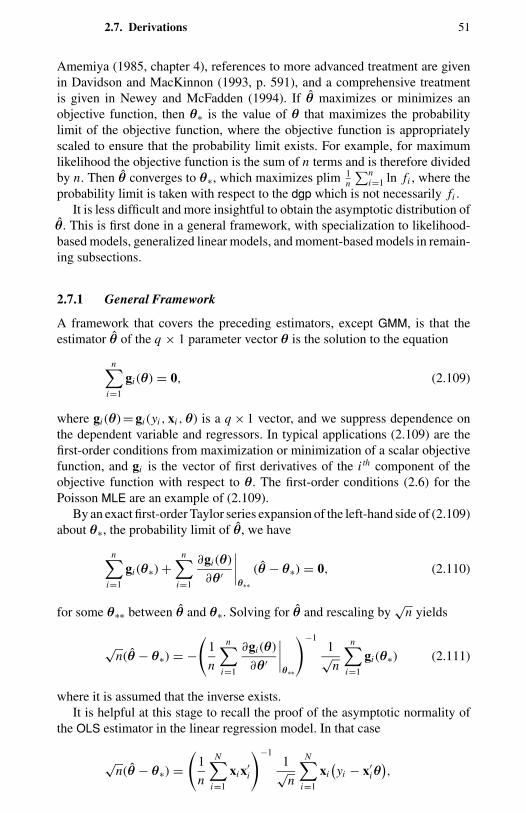
2.7. Derivations 51

Amemiya (1985, chapter 4), references to more advanced treatment are givenin Davidson and MacKinnon (1993, p. 591), and a comprehensive treatmentis given in Newey and McFadden (1994). If θ maximizes or minimizes anobjective function, then θ∗ is the value of θ that maximizes the probabilitylimit of the objective function, where the objective function is appropriatelyscaled to ensure that the probability limit exists. For example, for maximumlikelihood the objective function is the sum of n terms and is therefore dividedby n. Then θ converges to θ∗, which maximizes plim 1

n

∑ni=1 ln fi , where the

probability limit is taken with respect to the dgp which is not necessarily fi .It is less difficult and more insightful to obtain the asymptotic distribution of

θ. This is first done in a general framework, with specialization to likelihood-based models, generalized linear models, and moment-based models in remain-ing subsections.

2.7.1 General Framework

A framework that covers the preceding estimators, except GMM, is that theestimator θ of the q × 1 parameter vector θ is the solution to the equation

n∑i=1

gi (θ) = 0, (2.109)

where gi (θ) = gi (yi , xi ,θ) is a q × 1 vector, and we suppress dependence onthe dependent variable and regressors. In typical applications (2.109) are thefirst-order conditions from maximization or minimization of a scalar objectivefunction, and gi is the vector of first derivatives of the i th component of theobjective function with respect to θ. The first-order conditions (2.6) for thePoisson MLE are an example of (2.109).

By an exact first-order Taylor series expansion of the left-hand side of (2.109)about θ∗, the probability limit of θ, we have

n∑i=1

gi (θ∗) +n∑

i=1

∂gi (θ)

∂θ′

∣∣∣∣θ∗∗

(θ − θ∗) = 0, (2.110)

for some θ∗∗ between θ and θ∗. Solving for θ and rescaling by√

n yields

√n(θ − θ∗) = −

(1

n

n∑i=1

∂gi (θ)

∂θ′

∣∣∣∣θ∗∗

)−11√n

n∑i=1

gi (θ∗) (2.111)

where it is assumed that the inverse exists.It is helpful at this stage to recall the proof of the asymptotic normality of

the OLS estimator in the linear regression model. In that case

√n(θ − θ∗) =

(1

n

N∑i=1

xi x′i

)−11√n

N∑i=1

xi(yi − x′

iθ),

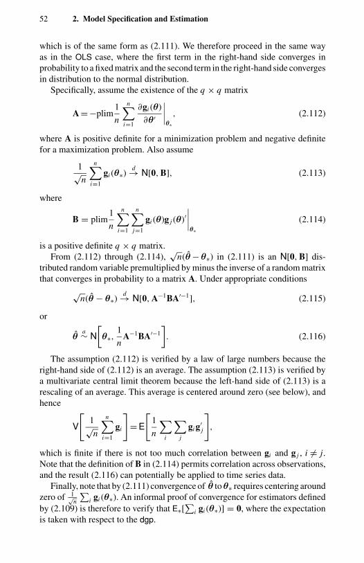
52 2. Model Specification and Estimation

which is of the same form as (2.111). We therefore proceed in the same wayas in the OLS case, where the first term in the right-hand side converges inprobability to a fixed matrix and the second term in the right-hand side convergesin distribution to the normal distribution.

Specifically, assume the existence of the q × q matrix

A = −plim1

n

n∑i=1

∂gi (θ)

∂θ′

∣∣∣∣θ∗

, (2.112)

where A is positive definite for a minimization problem and negative definitefor a maximization problem. Also assume

1√n

n∑i=1

gi (θ∗)d→ N[0, B], (2.113)

where

B = plim1

n

n∑i=1

n∑j=1

gi (θ)g j (θ)′∣∣∣∣θ∗

(2.114)

is a positive definite q × q matrix.From (2.112) through (2.114),

√n(θ−θ∗) in (2.111) is an N[0, B] dis-

tributed random variable premultiplied by minus the inverse of a random matrixthat converges in probability to a matrix A. Under appropriate conditions

√n(θ − θ∗)

d→ N[0, A−1BA′−1], (2.115)

or

θa∼ N[θ∗,

1

nA−1BA′−1

]. (2.116)

The assumption (2.112) is verified by a law of large numbers because theright-hand side of (2.112) is an average. The assumption (2.113) is verified bya multivariate central limit theorem because the left-hand side of (2.113) is arescaling of an average. This average is centered around zero (see below), andhence

V

[1√n

n∑i=1

gi

]= E

[1

n

∑i

∑j

gi g′j

],

which is finite if there is not too much correlation between gi and g j , i = j.Note that the definition of B in (2.114) permits correlation across observations,and the result (2.116) can potentially be applied to time series data.

Finally, note that by (2.111) convergence of θ toθ∗ requires centering aroundzero of 1√

n

∑i gi (θ∗). An informal proof of convergence for estimators defined

by (2.109) is therefore to verify that E∗[∑

i gi (θ∗)] = 0, where the expectationis taken with respect to the dgp.

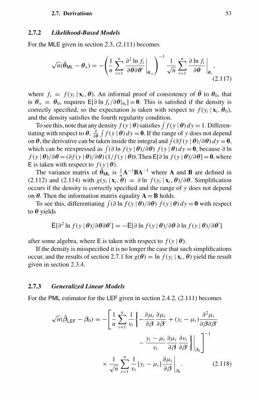
2.7. Derivations 53

2.7.2 Likelihood-Based Models

For the MLE given in section 2.3, (2.111) becomes

√n(θML − θ∗) = −

(1

n

n∑i=1

∂2 ln fi

∂θ∂θ′

∣∣∣∣θ∗∗

)−11√n

n∑i=1

∂ ln fi

∂θ

∣∣∣∣θ∗

,

(2.117)

where fi = f (yi | xi ,θ). An informal proof of consistency of θ to θ0, thatis θ∗ = θ0, requires E[∂ ln fi/∂θ|θ0 ] = 0. This is satisfied if the density iscorrectly specified, so the expectation is taken with respect to f (yi | xi ,θ0),and the density satisfies the fourth regularity condition.

To see this, note that any density f (y |θ) satisfies∫

f (y |θ) dy = 1. Differen-tiating with respect to θ, ∂

∂θ

∫f (y |θ) dy = 0. If the range of y does not depend

on θ, the derivative can be taken inside the integral and∫

(∂ f (y |θ)/∂θ) dy = 0,which can be reexpressed as

∫(∂ ln f (y |θ)/∂θ) f (y |θ) dy = 0, because ∂ ln

f (y |θ)/∂θ= (∂ f (y |θ)/∂θ) (1/ f (y |θ)). Then E[∂ ln f (y |θ)/∂θ] = 0, whereE is taken with respect to f (y |θ).

The variance matrix of θML is 1n A−1BA−1 where A and B are defined in

(2.112) and (2.114) with g(yi | xi ,θ) = ∂ ln f (yi | xi ,θ)/∂θ. Simplificationoccurs if the density is correctly specified and the range of y does not dependon θ. Then the information matrix equality A = B holds.

To see this, differentiating∫

(∂ ln f (y |θ)/∂θ) f (y |θ) dy = 0 with respectto θ yields

E[∂2 ln f (y |θ)/∂θ∂θ′] = −E[∂ ln f (y |θ)/∂θ ∂ ln f (y |θ)/∂θ′]

after some algebra, where E is taken with respect to f (y |θ).If the density is misspecified it is no longer the case that such simplifications

occur, and the results of section 2.7.1 for g(θ) = ln f (yi | xi ,θ) yield the resultgiven in section 2.3.4.

2.7.3 Generalized Linear Models

For the PML estimator for the LEF given in section 2.4.2, (2.111) becomes

√n(βLEF − β0) = −

[1

n

n∑i=1

1

vi

−∂µi

∂β

∂µi

∂β′ + (yi − µi )∂2µi

∂β∂β′

− yi − µi

vi

∂µi

∂β

∂vi

∂β′

∣∣∣∣β0

]−1

× 1√n

n∑i=1

1

viyi − µi ∂µi

∂β

∣∣∣∣β0

. (2.118)

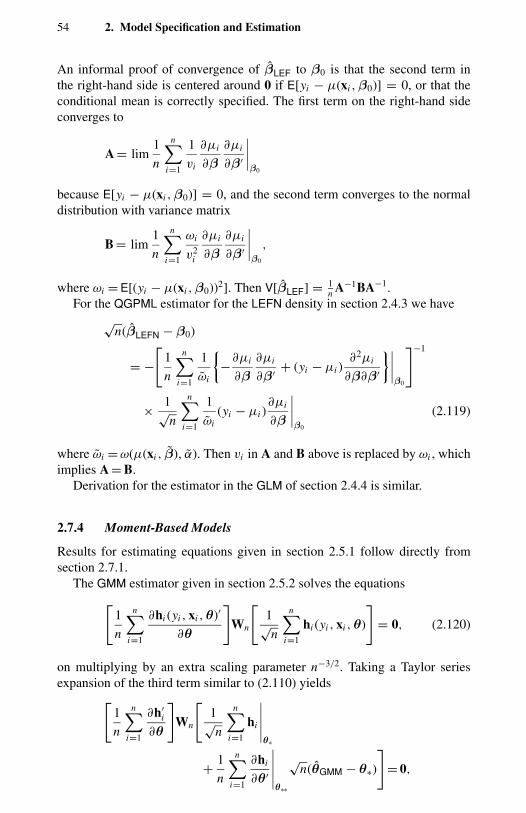
54 2. Model Specification and Estimation

An informal proof of convergence of βLEF to β0 is that the second term inthe right-hand side is centered around 0 if E[yi − µ(xi ,β0)] = 0, or that theconditional mean is correctly specified. The first term on the right-hand sideconverges to

A = lim1

n

n∑i=1

1

vi

∂µi

∂β

∂µi

∂β′

∣∣∣∣β0

because E[yi − µ(xi ,β0)] = 0, and the second term converges to the normaldistribution with variance matrix

B = lim1

n

n∑i=1

ωi

v2i

∂µi

∂β

∂µi

∂β′

∣∣∣∣β0

,

where ωi = E[(yi − µ(xi ,β0))2]. Then V[βLEF] = 1n A−1BA−1.

For the QGPML estimator for the LEFN density in section 2.4.3 we have√

n(βLEFN − β0)

= −[

1

n

n∑i=1

1

ωi

−∂µi

∂β

∂µi

∂β′ + (yi − µi )∂2µi

∂β∂β′

∣∣∣∣β0

]−1

× 1√n

n∑i=1

1

ωi(yi − µi )

∂µi

∂β

∣∣∣∣β0

(2.119)

where ωi = ω(µ(xi , β), α). Then vi in A and B above is replaced by ωi , whichimplies A = B.

Derivation for the estimator in the GLM of section 2.4.4 is similar.

2.7.4 Moment-Based Models

Results for estimating equations given in section 2.5.1 follow directly fromsection 2.7.1.

The GMM estimator given in section 2.5.2 solves the equations[1

n

n∑i=1

∂hi (yi , xi ,θ)′

∂θ

]Wn

[1√n

n∑i=1

hi (yi , xi ,θ)

]= 0, (2.120)

on multiplying by an extra scaling parameter n−3/2. Taking a Taylor seriesexpansion of the third term similar to (2.110) yields[

1

n

n∑i=1

∂h′i

∂θ

]Wn

[1√n

n∑i=1

hi

∣∣∣∣∣θ∗

+ 1

n

n∑i=1

∂hi

∂θ′

∣∣∣∣∣θ∗∗

√n(θGMM − θ∗)

]= 0,

2.7. Derivations 55

where hi = hi (yi , xi ,θ). Solving yields

√n(θGMM − θ∗) =

([1

n

n∑i=1

∂h′i

∂θ

]Wn

[1

n

n∑i=1

∂hi

∂θ′

∣∣∣∣θ∗

])−1

×[

1

n

n∑i=1

∂h′i

∂θ

]Wn

1√n

n∑i=1

hi

∣∣∣∣θ∗∗

. (2.121)

Equation (2.121) is the key result for obtaining the variance of the GMMestimator. It is sufficient to obtain the probability limit of the first five termsand the limit distribution of the last term in the right-hand side of (2.121). Both1n

∑i ∂hi/∂θ

′ and 1n

∑i ∂hi/∂θ

′|θ∗ converge in probability to the matrix Hdefined in (2.73), and by assumption plimWn = W. By a central limit theorem

1√n

∑i hi |θ∗∗ converges in distribution to N[0, S] where

S = limn→∞

1

nE

[∑i

∑j

hi h′j

∣∣∣∣θ∗

].

Thus from (2.121)√

n(θGMM −θ∗) has the same limit distribution as (H′WH)−1

H′W times a random variable that is N[0, S]. Equivalently,√

n(θ − θ∗)d→

N[0, A−1BA−1] where A = H′WH and B = H′WSWH.The optimal GMM estimator can be motivated by noting that the variance is

exactly the same matrix form as that of the linear WLS estimator given in (2.24),with X = H, V−1 = W and Ω= S. For given X and Ω the linear WLS variance isminimized by choosing V =Ω. By the same matrix algebra, for given H and Sthe GMM variance is minimized by choosing W = S−1. Analogously to feasibleGLS one can equivalently use Wn = S−1 where S is consistent for S.

2.7.5 Conditional Moment Tests

For the distribution of the conditional moment test statistic (2.96), we take afirst-order Taylor series expansion about θ0

1√n

m(θ) = 1√n

n∑i=1

mi (θ0) + 1

n

n∑i=1

∂mi (θ0)

∂θ′√

n(θ − θ0),

(2.122)

where mi (θ0) = mi (yi , xi ,θ0) and ∂mi (θ0)/∂θ′ = ∂mi (yi , xi ,θ0)/∂θ′|θ0 . Wesuppose θ is the solution to the first-order conditions

n∑i=1

gi (θ) = 0,

56 2. Model Specification and Estimation

where gi (θ) = gi (yi , xi ,θ). Replacing√

n(θ − θ0) by the right-hand side of(2.111) yields

1√n

m(θ) = 1√n

n∑i=1

mi (θ0) − 1

n

n∑i=1

∂mi (θ0)

∂θ′

×(

1

n

n∑i=1

∂gi (θ0)

∂θ′

)−11√n

n∑i=1

gi (θ0). (2.123)

It follows on some algebra that

1√n

m(θ)L D= [Ir −CA−1]

1√n

∑ni=1 mi (θ0)

1√n

∑ni=1 gi (θ0)

(2.124)

whereL D= means has the same limit distribution as, and

C = limn→∞

1

nE

[n∑

i=1

∂mi

∂θ′

∣∣∣∣θ0

],

and

A = limn→∞

1

nE

[n∑

i=1

∂gi

∂θ′

∣∣∣∣θ0

].

Equation (2.124) is the key to obtaining the distribution of the CM teststatistic. By a central limit theorem the second term in the right-hand side of(2.124) converges to N[0, J] where

J = limn→∞

1

nE

[∑ni=1 mi m′

i

∑ni=1 mi g′

i∑ni=1 gi m′

i

∑ni=1 gi g′

i

] ∣∣∣∣∣θ0

.

It follows that n−1/2m(θ)d→ N[0, Vm] where

Vm = HJH′,

J is defined already, and

H = [Ir −CA−1].The CM test can be operationalized by dropping the expectation and evaluatingthe expressions above at θ.

In the special case in which (2.104) holds, that is, E[∂mi/∂θ′] = 0, C = 0

so Vm = HJH′ = lim 1n E[∑n

i=1 mi m′i ] leading to the simplification (2.105). For

the OPG auxiliary regression (2.107) if θ is the MLE, see, for example, Paganand Vella (1989).

2.9 Exercises 57

2.8 Bibliographic Notes

Standard references for estimation theory are Amemiya (1985) and Davidsonand MacKinnon (1993), and a comprehensive treatment is given in Newey andMcFadden (1994). For maximum likelihood estimation see also Hendry (1995).The two-volume work by Gourieroux and Montfort (1995) presents estimationand testing theory in considerable detail, with considerable emphasis on the PMLframework. Reference to GLM is generally restricted to the statistics literature,even though it nests many common nonlinear regression models, including thelinear, logit, probit, and Poisson regression models. Key papers are Nelder andWedderburn (1972), Wedderburn (1974), and McCullagh (1983); the standardreference is McCullagh and Nelder (1989). The book by Fahrmeir and Tutz(1994) presents the GLM framework and recent advances in a form amenableto econometricians. This may encourage more social science analyses to takeadvantage of results for GLM models, especially for more complicated forms ofdata. The estimating equation approach is summarized by Carroll, Ruppert, andStefanski (1995). For GMM the paper by Hansen (1982) and other referencesare generally written at an advanced level. These include Newey and West(1987a), for a relatively brief statement of the estimator and its distribution, anddetailed textbook treatments by Ogaki (1993), Hamilton (1994, chapter 14), andDavidson and MacKinnon (1993, chapter 17).

2.9 Exercises

2.1 Let the dgp for y be y = Xβ0 + u, where X is nonstochastic and u ∼ (0,Ω).Show by substituting out y that the WLS estimator defined in (2.23) can be ex-pressed as βWLS = β0 + (X′V−1X)−1X′V−1u. Hence, obtain V[βWLS] givenin (2.24).

2.2 Let y have the LEF density f (y | µ) given in (2.26), where the rangeof the y does not depend on µ ≡ E[y]. Show by differentiating with respectto µ the identity

∫f (y | µ) dy = 1 that E[a′(µ) + c′(µ)y] = 0. Hence obtain

E[y] given in (2.27). Show by differentiating with respect to µ the identity∫y f (y | µ) dy = µ that E[a′(µ)y + c′(µ)y2] = 1. Hence, obtain V[y] given in

(2.28).

2.3 For the LEF log-likelihood defined in (2.29) and (2.30) obtain the first-order conditions for the MLE βML. Show that these can be reexpressed as (2.31)using (2.27) and (2.28). From (2.31) obtain the first-order conditions for theMLE of the Poisson regression model with exponential mean function.

2.4 Consider the geometric density f (y | µ) = µy(1 + µ)−y−1 , where y =0, 1, 2, . . . and µ = E[y]. Write this density in the LEF form (2.26). Hence,obtain the formula for V[y] using (2.28). In the regression case in whichµi = exp(x′

iβ) obtain the first-order conditions for the MLE for β. Give thedistribution for this estimator, assuming correct specification of the variance.

58 2. Model Specification and Estimation

2.5 Consider the geometric density f (y | µ) = µy(1 + µ)−y−1 , where y = 0, 1,2, . . . and µ = E[y]. Write this density in the canonical form of the LEF (2.45).Hence, obtain the formula for V[y] using (2.47). Obtain the canonical linkfunction for the geometric, verifying that it is not the log link function. Inthe regression case with the canonical link function obtain the first-order con-ditions for the MLE for β. Give the distribution for this estimator, assumingcorrect specification of the variance.

2.6 Models with exponential mean function exp(x′iβ), where β and xi are

k × 1 vectors, satisfy E[(yi − exp(x′iβ))xi ] = 0. Obtain the first-order condi-

tions for the GMM estimator that minimizes (2.68), where h(yi , xi ,β) = (yi −exp(x′

iβ))xi and W is k × k of rank k. Show that these first-order conditionsare a full-rank k × k matrix transformation of the first-order conditions (2.6)for the Poisson MLE. What do you conclude?

2.7 For the Poisson regression model with exponential mean function exp(x′

iβ), consider tests for exclusion of the subcomponent x2i of xi = [x′1i , x′

2i ]′,

which are tests of β2 = 0. Obtain the test statistic TLM given (2.88). State how tocompute an asymptotically equivalent version of the LM test using an auxiliaryregression. State how to alternatively implement Wald and LR tests of β2 = 0.

2.8 Show that variance–mean equality in the Poisson regression model withexponential mean implies that E[yi −exp(x′

iβ)2−yi 2] = 0. Using this momentcondition obtain the conditional moment test statistic TCM given in (2.105), firstshowing that the simplifying condition (2.104) holds if yi ∼ P[exp(x′

iβ)]. Statehow to compute TCM by an auxiliary regression. Does β need to be the MLEhere, or will any

√n-consistent estimator do?

CHAPTER 3

Basic Count Regression

3.1 Introduction

This chapter is intended to provide a self-contained treatment of basic cross-section count data regression analysis. It is analogous to a chapter in a standardstatistics text that covers both homoskedastic and heteroskedastic linear regres-sion models.

The most commonly used count models are Poisson and negative binomial.For readers interested only in these models it is sufficient to read sections 3.1through 3.5, along with preparatory material in sections 1.2 and 2.2 in previouschapters.

Additional regression models for cross-section count data are given in theremainder of Chapter 3, most notably the ordered probit and logit models. Theseadditional models generally ignore the count nature of the data. Still furthermodels, such as the hurdle model, which do explicitly treat the data as countdata, are given in Chapter 4. Some model diagnostic methods are presented inChapter 3, but most are deferred to Chapter 5.

As indicated in Chapter 2, the properties of an estimator vary with the as-sumptions made on the dgp. By correct specification of the conditional mean orvariance or density, we mean that the functional form and explanatory variablesin the specified conditional mean or variance or density are those of the dgp.

The simplest regression model for count data is the Poisson regression model.For the Poisson MLE it can be shown that:

1. Consistency requires correct specification of the conditional mean. Itdoes not require that the dependent variable y be Poisson distributed.

2. Valid statistical inference using computed maximum likelihood stan-dard errors and t statistics requires correct specification of both theconditional mean and variance. This requires equidispersion, that is,equality of conditional variance and mean, but not Poisson distributionfor y.

3. Valid statistical inference using appropriately modified maximum like-lihood output is still possible if data are not equidispersed, providedthe conditional mean is correctly specified.

60 3. Basic Count Regression

4. More efficient estimators than Poisson MLE can be obtained if dataare not equidispersed.

Properties 1 through 4 are similar to those of the OLS estimator in theclassical linear regression model, which is the MLE if errors are iid normal. ThePoisson restriction of equidispersion is directly analogous to homoskedasticityin the linear model. If errors are heteroskedastic in the linear model, one woulduse alternative t statistics to those from the usual OLS output (property 3) andpreferably estimate by WLS (property 4).

In many applications count data are overdispersed, with conditional vari-ance exceeding conditional mean. One response is to nonetheless use Poissonregression, because as already noted it still yields consistent estimates providedthe conditional mean is correctly specified. It is necessary, however, to adjuststandard error estimates. This leads to estimators closely related to the PoissonMLE, which differ according to assumptions made about the dgp. Specializingthe GLM results from Section 2.4 to the Poisson case, we have

1. Poisson MLE with statistical inference based on the assumption thatthe data are Poisson.

2. Poisson pseudo-MLE (PMLE), which is the Poisson MLE with statis-tical inference based on the correct specification of the mean but notassuming equidispersion.

3. Poisson GLM estimator, quasigeneralized PMLE (QGPMLE), and GMMestimator, which are all based on correct specification of the mean andvariance.

Results vary with the specified variance function. By far the simplest as-sumption is that the variance is a multiple of the mean. In this case the Poissonmaximum likelihood and GLM coefficient estimates are identical, and the usualPoisson maximum likelihood standard errors and t statistics can be used afterappropriate rescaling.

An alternative to Poisson regression is to specify a more general distributionthan the Poisson that does not impose equidispersion and to perform standardmaximum likelihood inference. The standard distribution used is the negativebinomial, with variance assumed to be a quadratic function of the mean.

It is important that such modifications to Poisson MLE be made. Count dataare often very overdispersed, which causes computed Poisson maximum likeli-hood t statistics to be considerably overinflated. This can lead to very erroneousand overly optimistic conclusions of statistical significance of regressors.

The various Poisson regression estimators are presented in section 3.2; neg-ative binomial regression is given in section 3.3. Tests for overdispersion arepresented in section 3.4. Practical issues of interpretation of coefficients withan exponential, rather than linear, specification of the conditional mean, anduse of estimates for prediction, are presented in section 3.5. An alternativeapproach to count data is to assume an underlying continuous latent process,with higher counts arising as the continuous variable passes successively higher

3.2. Poisson MLE, PMLE, and GLM 61

thresholds. Ordered probit and related discrete choice models are presented insection 3.6. Least-squares methods are the focus of section 3.7. These includenonlinear least squares with exponential conditional mean function, and OLSwith the dependent variable a transformation of the count data y to reduce het-eroskedasticity and asymmetry. Throughout this chapter the methods presentedare applied to a regression model for the number of doctor visits, introduced insection 3.2.6.

For completeness many different models, regression parameter estimators,and standard error estimators are presented in this chapter. The models consid-ered are the Poisson and two variants of the negative binomial – NB1 and NB2.The estimators considered include MLE, PMLE, and QGPMLE. An acronymsuch as NB1 MLE is shorthand for the NB1 model estimated by maximumlikelihood.

For many analyses the Poisson PMLE with corrected standard errors, thenegative binomial MLE, and the ordered probit MLE are sufficient. The mostcommon departure from these is the hurdle model, presented in the next chapter.

3.2 Poisson MLE, PMLE, and GLM

Many of the algebraic results presented in this chapter need to be modified ifthe conditional mean function is not exponential.

3.2.1 Poisson MLE

From section 1.2.3, the Poisson regression model specifies that yi given xi isPoisson distributed with density

f (yi | xi ) = e−µi µyi

i

yi !, yi = 0, 1, 2, . . . (3.1)

and mean parameter

E[yi | xi ] = µi = exp(x′

iβ). (3.2)

The specification (3.2) is called the exponential mean function. The modelcomprising (3.1) and (3.2) is usually referred to as the Poisson regression model,a terminology we also use, although more precisely it is the Poisson regressionmodel with exponential mean function. In the statistics literature the model isalso called a log-linear model, because the logarithm of the conditional meanis linear in the parameters: ln E[yi | xi ] = x′

iβ.Given independent observations, the log-likelihood is

ln L(β) =n∑

i=1

yi x′

iβ − exp(x′

iβ)− ln yi !

. (3.3)

62 3. Basic Count Regression

The Poisson MLE βP is the solution to the first-order conditions

n∑i=1

(yi − exp

(x′

iβ))

xi = 0. (3.4)

Note that if the regressors include a constant term then the residuals yi−exp (x′

iβ) sum to zero by (3.4).The standard method for computation of βP is the Newton-Raphson itera-

tive method. Convergence is guaranteed, because the log-likelihood functionis globally concave. In practice often fewer than ten iterations are needed. TheNewton-Raphson method can be implemented by iterative use of OLS as pre-sented in section 3.8.

If the dgp for yi is indeed Poisson with mean (3.2) we can apply the usualmaximum likelihood theory as in section 2.3.2. This yields

βPa∼ N[β, VML[βP]] (3.5)

where

VML[βP] =(

n∑i=1

µi xi x′i

)−1

, (3.6)

using E[∂2 ln L/∂β∂β′] = −∑ni=1 µi xi x′

i . Strictly speaking we should assumethat the dgp evaluates β at the specific value β0 and replace β by β0 in (3.5).This more formal presentation is used in Chapter 2. In the rest of the book weuse a less formal presentation, provided the estimator is indeed consistent.

Most statistical programs use Hessian maximum likelihood (MLH) stan-dard errors using (3.6) evaluated at µi = exp(x′

i βP). By the information matrixequality one can instead use the summed outer product of the first derivatives(see section 2.3.2), leading to the maximum likelihood outer product (MLOP)estimator

VMLOP[βP] =(

n∑i=1

(yi − µi )2xi x′

i

)−1

, (3.7)

evaluated at µi . A general optimization routine may provide standard errorsbased on (3.7), which asymptotically equals (3.6) if data are equidispersed.

3.2.2 NB1 and NB2 Variance Functions

In the Poisson regression model yi has mean µi = exp(x′iβ) and variance µi .

We now relax the variance assumption, because data almost always reject therestriction that the variance equals the mean, and we maintain the assumptionthat the mean is exp(x′

iβ).We use the general notation

ωi = V[yi | xi ] (3.8)

3.2. Poisson MLE, PMLE, and GLM 63

to denote the conditional variance of yi . It is natural to continue to model thevariance as a function of the mean, with

ωi = ω(µi , α) (3.9)

for some specified function ω(·) and where α is a scalar parameter. Most modelsspecialize this to the general variance function

ωi = µi + αµpi , (3.10)

where the constant p is specified. Analysis is usually restricted to two specialcases, in addition to the Poisson case of α = 0.

First, the NB1 variance function sets p = 1. Then the variance

ωi = (1 + α)µi (3.11)

is a multiple of the mean. In the GLM framework this is usually rewritten as

ωi = φµi , (3.12)

where φ = 1 + α.Second, the NB2 variance function sets p = 2. Then the variance is quadratic

in the mean:

ωi = µi + αµ2i . (3.13)

In both cases the dispersion parameter α is to be estimated.Cameron and Trivedi (1986), in the context of negative binomial models,

used the terminology NB1 model to describe the case p = 1 and NB2 model todescribe the case p = 2. Here we have extended this terminology to the variancefunction itself.

3.2.3 Poisson PMLE

The assumption of a Poisson distribution is stronger than necessary for sta-tistical inference based on βP defined by (3.4). As discussed in section 2.4.2,whose results are used extensively in this subsection, consistency holds forthe MLE of any specified LEF density such as the Poisson, provided the con-ditional mean function (3.2) is correctly specified. An intuitive explanation isthat consistency requires the left-hand side of the first-order conditions (3.4)to have expected value zero. This is the case if E[yi | xi ] = exp(x′

iβ), becausethen E[(yi − exp(x′

iβ))xi ] = 0.Given this robustness to distributional assumptions, we can continue to use

βP even if the dgp for yi is not the Poisson. If an alternative dgp is entertained,the estimator defined by the Poisson maximum likelihood first-order conditions(3.4) is called the Poisson pseudo-MLE (PMLE) or the Poisson quasi-MLE. Thisterminology means that the estimator is like the Poisson MLE in that the Poissonmodel is used to motivate the first-order condition defining the estimator, but it

64 3. Basic Count Regression

is unlike the Poisson MLE in that the dgp used to obtain the distribution of theestimator need not be the Poisson. Here we assume the Poisson mean but relaxthe Poisson restriction of equidispersion.

The Poisson PMLE βP is defined to be the solution to (3.4). If (3.2) holdsthen

βPa∼ N[β, VPML[βP]], (3.14)

where

VPML[βP] =(

n∑i=1

µi xi x′i

)−1 ( n∑i=1

ωi xi x′i

)(n∑

i=1

µi xi x′i

)−1

(3.15)

and ωi is the conditional variance of yi defined in (3.8). Implementation of(3.15) depends on what functional form, if any, is assumed for ωi .

Poisson PMLE with Poisson Variance Function

If the conditional variance of yi is that for the Poisson, so ωi = µi , then thevariance matrix (3.15) simplifies to (3.6). Thus the usual Poisson maximum like-lihood inference is valid provided the first two moments are correctly specified.

Poisson PMLE with NB1 Variance Function

The simplest generalization of ωi = µi is the NB1 variance function (3.12).Because ωi = φµi the variance matrix in (3.15) simplifies to

VNB1[βP] = φ

(n∑

i=1

µi xi x′i

)−1

= φVML[βP], (3.16)

where VML[βP] is the maximum likelihood variance matrix given in (3.6). Thus,the simplest way to handle overdispersed or underdispersed data is to begin withthe computed Poisson maximum likelihood output. Then, multiply maximumlikelihood output by φ to obtain correct variance matrix, multiply by

√φ to

obtain correct standard errors, and divide by√

φ to get correct t statistics.The standard estimator of φ is

φNB1 = 1

n − k

n∑i=1

(yi − µi )2

µi. (3.17)

The motivation for this estimator is that variance function (3.12) implies E[(yi −µi )2] = φµi and hence φ = E[(yi − µi )2/µi ]. The corresponding sample mo-ment is (3.17) where division by (n − k) rather than n is a degrees-of-freedomcorrection. This approach to estimation is the GLM approach presented insection 2.4.3; see also section 3.2.4. Poisson regression packages using the

3.2. Poisson MLE, PMLE, and GLM 65

GLM framework automatically use (3.16) for standard errors; most others in-stead use (3.6).

Poisson PMLE with NB2 Variance Function

A common alternative specification for the variance of yi is the NB2 variancefunction (3.13). Then, because ωi = µi + αµ2

i , the variance matrix (3.15) be-comes

VNB2[βP] =(

n∑i=1

µi xi x′i

)−1( n∑i=1

(µi + αµ2

i

)xi x′

i

)(n∑

i=1

µi xi x′i

)−1

.

(3.18)

This does not simplify and computation requires matrix routines. One of severalpossible estimators of α is

αNB2 = 1

n − k

n∑i=1

(yi − µi )2 − µi µ2

i

. (3.19)

The motivation for this estimator of α is that (3.13) implies E[(yi −µi )2 −µi ] =αµ2

i and hence α = E[(yi − µi )2 − µi /µ2i ]. The corresponding sample mo-

ment with degrees-of-freedom correction is (3.19). This estimator was proposedby Gourieroux et al. (1984a, 1984b).

Alternative estimators of φ and α for NB1 and NB2 variance functions aregiven in Cameron and Trivedi (1986). In practice studies do not present esti-mated standard errors for φNB1 and αNB2, although these can be obtained usingthe delta method given in section 2.6.2. A series of papers by Dean (1993,1994) and Dean, Eaves and Martinez (1995) consider different estimators forthe dispersion parameter and consequences for variance matrix estimation.

Poisson PMLE with Unspecified Variance Function

The variance matrix (3.15) can be consistently estimated without specifica-tion of a functional form for ωi . We need to estimate for unknown ωi themiddle term in VPML[βP] defined in (3.15). Formally, a consistent estimate oflim 1

n

∑ni=1 E[(yi − µi )2 | xi ]xi x′

i is needed. It can be shown that if (yi , xi ) areiid this k × k matrix is consistently estimated by 1

n

∑ni=1(yi − µi )2xi x′

i , eventhough it is impossible to consistently estimate each of the n scalars ω2

i by(yi − µi )2. This yields the variance matrix estimate

VRS[βP] =(

n∑i=1

µi xi x′i

)−1 ( n∑i=1

(yi − µi )2xi x′

i

)(n∑

i=1

µi xi x′i

)−1

,

(3.20)

which is evaluated at µi .

66 3. Basic Count Regression

The estimator (3.20) is the RS estimator discussed in section 2.5.1. It buildson work by Eicker (1967), who obtained a similar result in the nonregressioncase, and White (1980), who obtained this result in the OLS regression caseand popularized its use in econometrics. See Robinson (1987) for a historyof this approach and for further references. This method is used extensivelythroughout this book, in settings much more general than the Poisson PMLEwith cross-section data. As shorthand we refer to standard errors as robuststandard errors whenever a similar approach is used to obtain standard errorswithout specifying functional forms for the second moments of the dependentvariable.

An alternative way to proceed when the variance function ωi is not specifiedis to bootstrap. This estimates properties of the distribution of βP and performsstatistical inference on β by resampling from the original data set. The standardprocedure for linear regression is to bootstrap residuals (yi −µi ). This procedurecannot be applied to residuals from Poisson regression, however, as (yi − µi )is then heteroskedastic, and noninteger values of yi would arise. Instead forPoisson regression we bootstrap the pairs (yi , xi ). A detailed discussion of thebootstrap is given in section 5.5.1.

3.2.4 Poisson GLM

Generalized linear models are defined in section 2.4.4. For the Poisson withmean function (3.2), which is the canonical link function for this model, thePoisson GLM density is

f (yi | xi ) = exp

x′

iβyi − exp(x′

iβ)

φ+ c(yi , φ)

, (3.21)

where c(yi , φ) is a normalizing constant. Then V[yi ] = φµi , which is the NB1variance function.

The Poisson GLM estimator βPGLM maximizes with respect to β the corre-sponding log-likelihood, with first-order conditions

n∑i=1

1

φ

(yi − exp

(x′

iβ))

xi = 0. (3.22)

These coincide with (3.4) for the Poisson PML, except for scaling by the constantφ. Consequently βPGLM = βP, and the variance matrix is the same as (3.16)for the Poisson PML with NB1 variance function

V[βPGLM] = φ

(n∑

i=1

µi xi x′i

)−1

. (3.23)

To implement this last result for statistical inference on β, GLM practitionersuse the consistent estimate φNB1 defined in (3.17).

3.2. Poisson MLE, PMLE, and GLM 67

A more obvious approach to estimating the nuisance parameter φ is to max-imize the log-likelihood based on (3.21) with respect to both β and φ. Differ-entiation with respect to φ requires an expression for the normalizing constantc(yi , φ), however, and the restriction that probabilities sum to unity,

∞∑yi =0

exp

1

φ

(x′

iβyi − exp(x′

iβ))+ c(yi , φ)

= 1,

has no simple solution for c(yi , φ). One therefore uses the estimator (3.17),which is based on assumptions about the first two moments rather than thedensity. More generally the density (3.21) is best thought of as merely givinga justification for the first-order conditions (3.22), rather than as a density thatwould be used, for example, to predict the probabilities of particular valuesof y.

3.2.5 Poisson EE

A quite general estimation procedure is to use the estimating equation presentedin section 2.4.5,∑

i

1

ωi(yi − µi )

∂µi

∂β= 0,

which generalizes linear WLS. Consider a specific variance function of the formωi = ω(µi , α), and let α be a consistent estimator of α. For the exponential meanfunction ∂µi/∂β = µi xi , so βEE solves the first-order conditions

n∑i=1

1

ω(µi , α)(yi − µi )µi xi = 0. (3.24)

If the variance function is correctly specified then it follows that

VEE[βEE] =(

n∑i=1

1

ω(µi , α)µ2

i xi x′i

)−1

. (3.25)

Because this estimator is motivated by specification of the first two moments,it can also be viewed as a method-of-moments estimator, a special case of GMMwhose more general framework is unnecessary here as the number of equations(3.24) equals the number of unknowns. The first-order conditions nest as specialcases those for the Poisson MLE and GLM, which replace ω(µi , α) by µi .

3.2.6 Example: Doctor Visits

Consider the following example of the number of doctor visits in the past 2weeks for a single-adult sample of size 5190 from the Australian Health Survey1977–78. This and several other measures of health service utilization such as

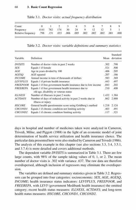
68 3. Basic Count Regression

Table 3.1. Doctor visits: actual frequency distribution

Count 0 1 2 3 4 5 6 7 8 9Frequency 4141 782 174 30 24 9 12 12 5 1Relative frequency .798 .151 .033 .006 .005 .002 .002 .002 .001 .000

Table 3.2. Doctor visits: variable definitions and summary statistics

StandardVariable Definition Mean deviation

DVISITS Number of doctor visits in past 2 weeks .302 .798SEX Equals 1 if female .521 .500AGE Age in years divided by 100 .406 .205AGESQ AGE squared .207 .186INCOME Annual income in tens of thousands of dollars .583 .369LEVYPLUS Equals 1 if private health insurance .443 .497FREEPOOR Equals 1 if free government health insurance due to low income .043 .202FREEREPA Equals 1 if free government health insurance due to .210 .408

old age, disability or veteran statusILLNESS Number of illnesses in past 2 weeks 1.432 1.384ACTDAYS Number of days of reduced activity in past 2 weeks due to .862 2.888

illness or injuryHSCORE General health questionnaire score using Goldberg’s method 1.218 2.124CHCOND1 Equals 1 if chronic condition not limiting activity .403 .491CHCOND2 Equals 1 if chronic condition limiting activity .117 .321

days in hospital and number of medicines taken were analyzed in Cameron,Trivedi, Milne, and Piggott (1988) in the light of an economic model of jointdetermination of health service utilization and health insurance choice. Theparticular data presented here were also studied by Cameron and Trivedi (1986).The analysis of this example in this chapter (see also sections 3.3, 3.4, 3.5.1,and 3.7.4) is more detailed and covers additional methods.

The dependent variable DVISITS is summarized in Table 3.1. There are fewlarge counts, with 98% of the sample taking values of 0, 1, or 2. The meannumber of doctor visits is .302 with variance .637. The raw data are thereforeoverdispersed, although inclusion of regressors may eliminate the overdisper-sion.

The variables are defined and summary statistics given in Table 3.2. Regres-sors can be grouped into four categories: socioeconomic: SEX, AGE, AGESQ,INCOME; health insurance status indicators: LEVYPLUS, FREEPOOR, andFREEREPA, with LEVY (government Medibank health insurance) the omittedcategory; recent health status measures: ILLNESS, ACTDAYS; and long-termhealth status measures: HSCORE, CHCOND1, CHCOND2.

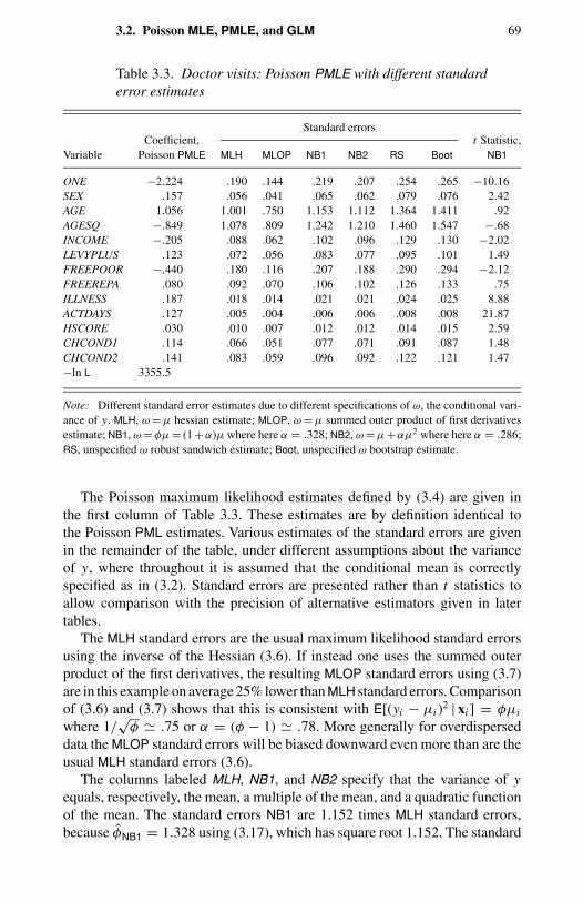
3.2. Poisson MLE, PMLE, and GLM 69

Table 3.3. Doctor visits: Poisson PMLE with different standarderror estimates

Standard errorsCoefficient, t Statistic,

Variable Poisson PMLE MLH MLOP NB1 NB2 RS Boot NB1

ONE −2.224 .190 .144 .219 .207 .254 .265 −10.16SEX .157 .056 .041 .065 .062 .079 .076 2.42AGE 1.056 1.001 .750 1.153 1.112 1.364 1.411 .92AGESQ −.849 1.078 .809 1.242 1.210 1.460 1.547 −.68INCOME −.205 .088 .062 .102 .096 .129 .130 −2.02LEVYPLUS .123 .072 .056 .083 .077 .095 .101 1.49FREEPOOR −.440 .180 .116 .207 .188 .290 .294 −2.12FREEREPA .080 .092 .070 .106 .102 .126 .133 .75ILLNESS .187 .018 .014 .021 .021 .024 .025 8.88ACTDAYS .127 .005 .004 .006 .006 .008 .008 21.87HSCORE .030 .010 .007 .012 .012 .014 .015 2.59CHCOND1 .114 .066 .051 .077 .071 .091 .087 1.48CHCOND2 .141 .083 .059 .096 .092 .122 .121 1.47−ln L 3355.5

Note: Different standard error estimates due to different specifications of ω, the conditional vari-ance of y. MLH, ω = µ hessian estimate; MLOP, ω = µ summed outer product of first derivativesestimate; NB1, ω = φµ = (1 +α)µ where here α = .328; NB2, ω = µ+αµ2 where here α = .286;RS, unspecified ω robust sandwich estimate; Boot, unspecified ω bootstrap estimate.

The Poisson maximum likelihood estimates defined by (3.4) are given inthe first column of Table 3.3. These estimates are by definition identical tothe Poisson PML estimates. Various estimates of the standard errors are givenin the remainder of the table, under different assumptions about the varianceof y, where throughout it is assumed that the conditional mean is correctlyspecified as in (3.2). Standard errors are presented rather than t statistics toallow comparison with the precision of alternative estimators given in latertables.

The MLH standard errors are the usual maximum likelihood standard errorsusing the inverse of the Hessian (3.6). If instead one uses the summed outerproduct of the first derivatives, the resulting MLOP standard errors using (3.7)are in this example on average 25% lower than MLH standard errors. Comparisonof (3.6) and (3.7) shows that this is consistent with E[(yi − µi )2 | xi ] = φµi

where 1/√

φ .75 or α = (φ − 1) .78. More generally for overdisperseddata the MLOP standard errors will be biased downward even more than are theusual MLH standard errors (3.6).

The columns labeled MLH, NB1, and NB2 specify that the variance of yequals, respectively, the mean, a multiple of the mean, and a quadratic functionof the mean. The standard errors NB1 are 1.152 times MLH standard errors,because φNB1 = 1.328 using (3.17), which has square root 1.152. The standard

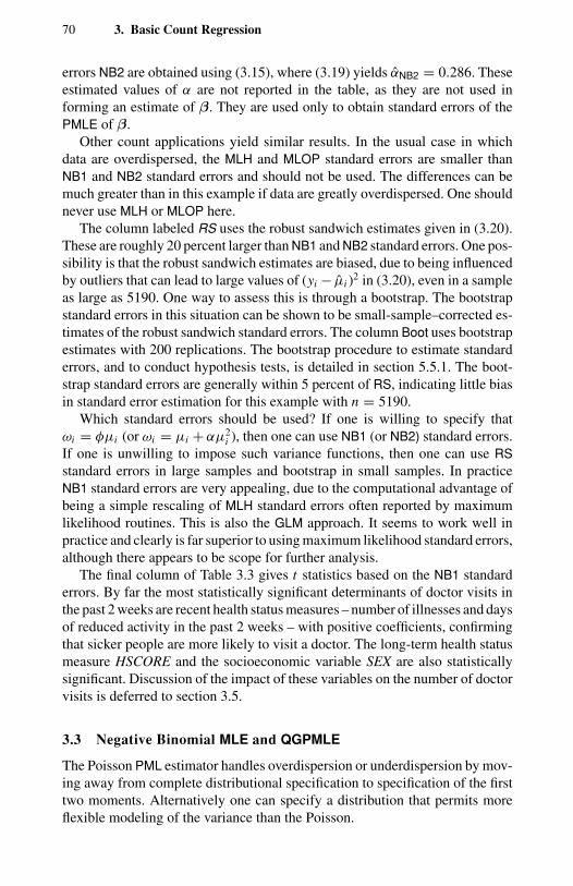
70 3. Basic Count Regression

errors NB2 are obtained using (3.15), where (3.19) yields αNB2 = 0.286. Theseestimated values of α are not reported in the table, as they are not used informing an estimate of β. They are used only to obtain standard errors of thePMLE of β.

Other count applications yield similar results. In the usual case in whichdata are overdispersed, the MLH and MLOP standard errors are smaller thanNB1 and NB2 standard errors and should not be used. The differences can bemuch greater than in this example if data are greatly overdispersed. One shouldnever use MLH or MLOP here.

The column labeled RS uses the robust sandwich estimates given in (3.20).These are roughly 20 percent larger than NB1 and NB2 standard errors. One pos-sibility is that the robust sandwich estimates are biased, due to being influencedby outliers that can lead to large values of (yi − µi )2 in (3.20), even in a sampleas large as 5190. One way to assess this is through a bootstrap. The bootstrapstandard errors in this situation can be shown to be small-sample–corrected es-timates of the robust sandwich standard errors. The column Boot uses bootstrapestimates with 200 replications. The bootstrap procedure to estimate standarderrors, and to conduct hypothesis tests, is detailed in section 5.5.1. The boot-strap standard errors are generally within 5 percent of RS, indicating little biasin standard error estimation for this example with n = 5190.

Which standard errors should be used? If one is willing to specify thatωi = φµi (or ωi = µi + αµ2

i ), then one can use NB1 (or NB2) standard errors.If one is unwilling to impose such variance functions, then one can use RSstandard errors in large samples and bootstrap in small samples. In practiceNB1 standard errors are very appealing, due to the computational advantage ofbeing a simple rescaling of MLH standard errors often reported by maximumlikelihood routines. This is also the GLM approach. It seems to work well inpractice and clearly is far superior to using maximum likelihood standard errors,although there appears to be scope for further analysis.

The final column of Table 3.3 gives t statistics based on the NB1 standarderrors. By far the most statistically significant determinants of doctor visits inthe past 2 weeks are recent health status measures – number of illnesses and daysof reduced activity in the past 2 weeks – with positive coefficients, confirmingthat sicker people are more likely to visit a doctor. The long-term health statusmeasure HSCORE and the socioeconomic variable SEX are also statisticallysignificant. Discussion of the impact of these variables on the number of doctorvisits is deferred to section 3.5.

3.3 Negative Binomial MLE and QGPMLE

The Poisson PML estimator handles overdispersion or underdispersion by mov-ing away from complete distributional specification to specification of the firsttwo moments. Alternatively one can specify a distribution that permits moreflexible modeling of the variance than the Poisson.

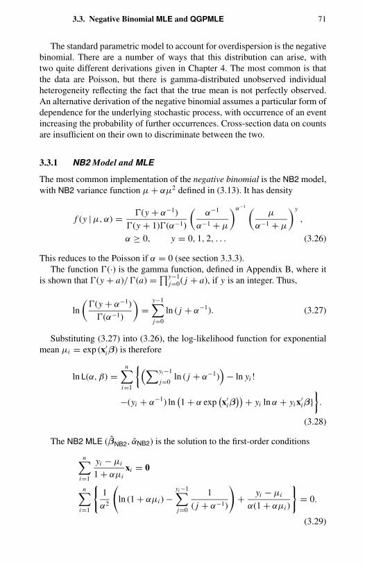
3.3. Negative Binomial MLE and QGPMLE 71

The standard parametric model to account for overdispersion is the negativebinomial. There are a number of ways that this distribution can arise, withtwo quite different derivations given in Chapter 4. The most common is thatthe data are Poisson, but there is gamma-distributed unobserved individualheterogeneity reflecting the fact that the true mean is not perfectly observed.An alternative derivation of the negative binomial assumes a particular form ofdependence for the underlying stochastic process, with occurrence of an eventincreasing the probability of further occurrences. Cross-section data on countsare insufficient on their own to discriminate between the two.

3.3.1 NB2 Model and MLE

The most common implementation of the negative binomial is the NB2 model,with NB2 variance function µ + αµ2 defined in (3.13). It has density

f (y | µ, α) = (y + α−1)

(y + 1)(α−1)

(α−1

α−1 + µ

)α−1 (µ

α−1 + µ

)y

,

α ≥ 0, y = 0, 1, 2, . . . (3.26)

This reduces to the Poisson if α = 0 (see section 3.3.3).The function (·) is the gamma function, defined in Appendix B, where it

is shown that (y + a)/(a) =∏y−1j=0( j + a), if y is an integer. Thus,

ln

((y + α−1)

(α−1)

)=

y−1∑j=0

ln ( j + α−1). (3.27)

Substituting (3.27) into (3.26), the log-likelihood function for exponentialmean µi = exp (x′

iβ) is therefore

ln L(α, β) =n∑

i=1

(∑yi −1

j=0ln ( j + α−1)

)− ln yi !

−(yi + α−1) ln(1 + α exp

(x′

iβ))+ yi ln α + yi x′

iβ.

(3.28)

The NB2 MLE (βNB2, αNB2) is the solution to the first-order conditions

n∑i=1

yi − µi

1 + αµixi = 0

n∑i=1

1

α2

(ln (1 + αµi ) −

yi −1∑j=0

1

( j + α−1)

)+ yi − µi

α(1 + αµi )

= 0.

(3.29)

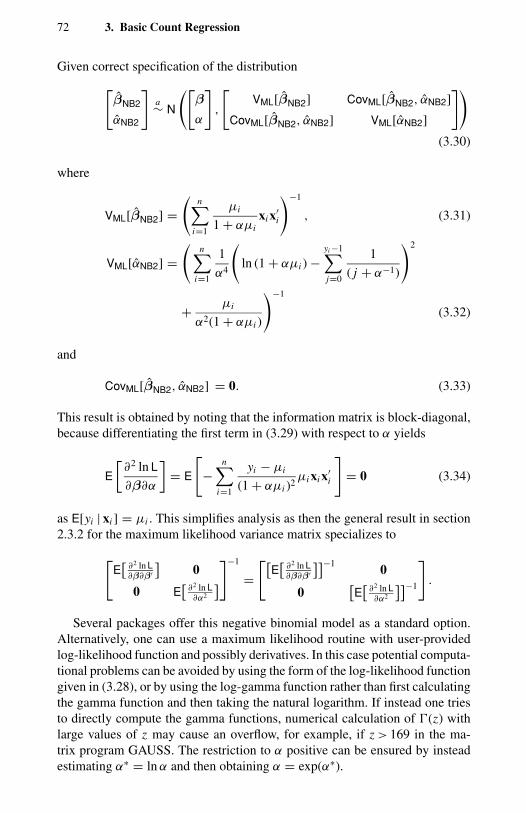
72 3. Basic Count Regression

Given correct specification of the distribution[βNB2

αNB2

]a∼ N

([β

α

],

[VML[βNB2] CovML[βNB2, αNB2]

CovML[βNB2, αNB2] VML[αNB2]

])(3.30)

where

VML[βNB2] =(

n∑i=1

µi

1 + αµixi x′

i

)−1

, (3.31)

VML[αNB2] =(

n∑i=1

1

α4

(ln (1 + αµi ) −

yi −1∑j=0

1

( j + α−1)

)2

+ µi

α2(1 + αµi )

)−1

(3.32)

and

CovML[βNB2, αNB2] = 0. (3.33)

This result is obtained by noting that the information matrix is block-diagonal,because differentiating the first term in (3.29) with respect to α yields

E

[∂2 ln L

∂β∂α

]= E

[−

n∑i=1

yi − µi

(1 + αµi )2µi xi x′

i

]= 0 (3.34)

as E[yi | xi ] = µi . This simplifies analysis as then the general result in section2.3.2 for the maximum likelihood variance matrix specializes to[

E[

∂2 ln L∂β∂β′

]0

0 E[

∂2 ln L∂α2

]]−1

=[[

E[

∂2 ln L∂β∂β′

]]−10

0[E[

∂2 ln L∂α2

]]−1

].

Several packages offer this negative binomial model as a standard option.Alternatively, one can use a maximum likelihood routine with user-providedlog-likelihood function and possibly derivatives. In this case potential computa-tional problems can be avoided by using the form of the log-likelihood functiongiven in (3.28), or by using the log-gamma function rather than first calculatingthe gamma function and then taking the natural logarithm. If instead one triesto directly compute the gamma functions, numerical calculation of (z) withlarge values of z may cause an overflow, for example, if z > 169 in the ma-trix program GAUSS. The restriction to α positive can be ensured by insteadestimating α∗ = ln α and then obtaining α = exp(α∗).

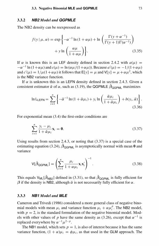
3.3. Negative Binomial MLE and QGPMLE 73

3.3.2 NB2 Model and QGPMLE

The NB2 density can be reexpressed as

f (y | µ, α) = exp

−α−1 ln (1 + αµ) + ln

((y + α−1)

(y + 1)(α−1)

)+ y ln

(αµ

1 + αµ

). (3.35)

If α is known this is an LEF density defined in section 2.4.2 with a(µ) =−α−1 ln (1+αµ) and c(µ) = ln (αµ/(1+αµ)). Because a′(µ) = −1/(1+αµ)and c′(µ) = 1/µ(1+αµ) it follows that E[y] = µ and V[y] = µ+αµ2, whichis the NB2 variance function.

If α is unknown this is an LEFN density defined in section 2.4.3. Given aconsistent estimator α of α, such as (3.19), the QGPMLE βQGPML maximizes

ln LLEFN =n∑

i=1

−α−1 ln (1 + αµi ) + yi ln

(αµi

1 + αµi

)+ b(yi , α)

.

(3.36)

For exponential mean (3.4) the first-order conditions are

n∑i=1

yi − µi

1 + αµixi = 0. (3.37)

Using results from section 2.4.3, or noting that (3.37) is a special case of theestimating equation (3.24), βQGPML is asymptotically normal with mean 0 andvariance

V[βQGPML] =(

n∑i=1

µi

1 + αµixi x′

i

)−1

. (3.38)

This equals VML[βNB2] defined in (3.31), so that βQGPML is fully efficient forβ if the density is NB2, although α is not necessarily fully efficient for α.

3.3.3 NB1 Model and MLE

Cameron and Trivedi (1986) considered a more general class of negative bino-mial models with mean µi and variance function µi + αµ

pi . The NB2 model,

with p = 2, is the standard formulation of the negative binomial model. Mod-els with other values of p have the same density as (3.26), except that α−1 isreplaced everywhere by α−1µ2−p.

The NB1 model, which sets p = 1, is also of interest because it has the samevariance function, (1 + α)µi = φµi , as that used in the GLM approach. The

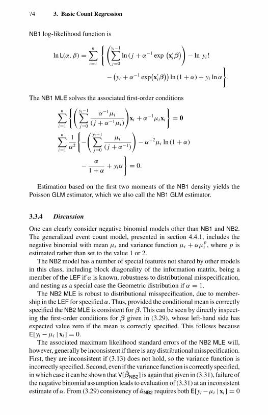
74 3. Basic Count Regression

NB1 log-likelihood function is

ln L(α, β) =n∑

i=1

(yi −1∑j=0

ln ( j + α−1 exp(x′

iβ))− ln yi !

− (yi + α−1 exp(x′

iβ))

ln (1 + α) + yi ln α

.

The NB1 MLE solves the associated first-order conditions

n∑i=1

(yi −1∑j=0

α−1µi

( j + α−1µi )

)xi + α−1µi xi

= 0

n∑i=1

1

α2

−(

yi −1∑j=0

µi

( j + α−1)

)− α−2µi ln (1 + α)

− α

1 + α+ yiα

= 0.

Estimation based on the first two moments of the NB1 density yields thePoisson GLM estimator, which we also call the NB1 GLM estimator.

3.3.4 Discussion

One can clearly consider negative binomial models other than NB1 and NB2.The generalized event count model, presented in section 4.4.1, includes thenegative binomial with mean µi and variance function µi + αµ

pi , where p is

estimated rather than set to the value 1 or 2.The NB2 model has a number of special features not shared by other models

in this class, including block diagonality of the information matrix, being amember of the LEF if α is known, robustness to distributional misspecification,and nesting as a special case the Geometric distribution if α = 1.

The NB2 MLE is robust to distributional misspecification, due to member-ship in the LEF for specified α. Thus, provided the conditional mean is correctlyspecified the NB2 MLE is consistent for β. This can be seen by directly inspect-ing the first-order conditions for β given in (3.29), whose left-hand side hasexpected value zero if the mean is correctly specified. This follows becauseE[yi − µi | xi ] = 0.

The associated maximum likelihood standard errors of the NB2 MLE will,however, generally be inconsistent if there is any distributional misspecification.First, they are inconsistent if (3.13) does not hold, so the variance function isincorrectly specified. Second, even if the variance function is correctly specified,in which case it can be shown that V[βNB2] is again that given in (3.31), failure ofthe negative binomial assumption leads to evaluation of (3.31) at an inconsistentestimate of α. From (3.29) consistency of αNB2 requires both E[yi −µi | xi ] = 0

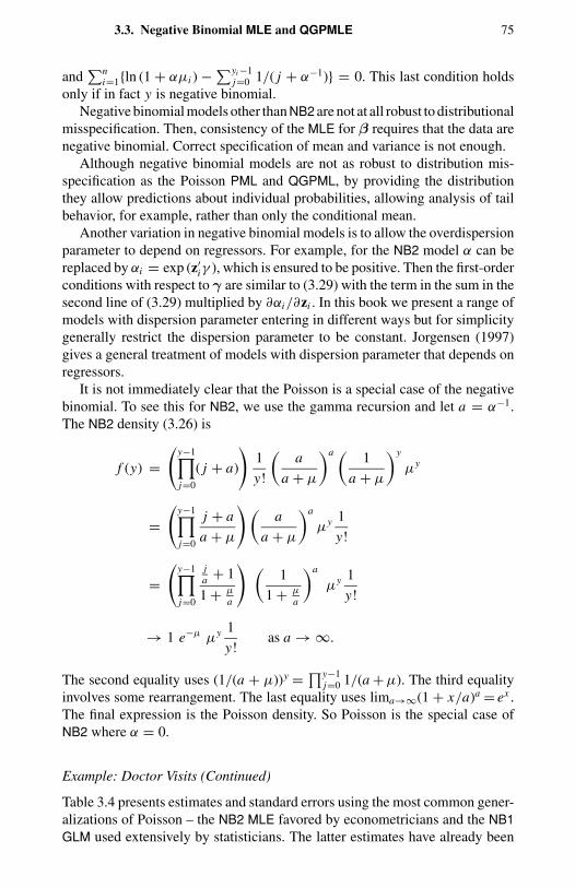
3.3. Negative Binomial MLE and QGPMLE 75

and∑n

i=1ln (1 + αµi ) −∑yi −1j=0 1/( j + α−1) = 0. This last condition holds

only if in fact y is negative binomial.Negative binomial models other than NB2 are not at all robust to distributional

misspecification. Then, consistency of the MLE for β requires that the data arenegative binomial. Correct specification of mean and variance is not enough.

Although negative binomial models are not as robust to distribution mis-specification as the Poisson PML and QGPML, by providing the distributionthey allow predictions about individual probabilities, allowing analysis of tailbehavior, for example, rather than only the conditional mean.

Another variation in negative binomial models is to allow the overdispersionparameter to depend on regressors. For example, for the NB2 model α can bereplaced by αi = exp (z′

iγ ), which is ensured to be positive. Then the first-orderconditions with respect to γ are similar to (3.29) with the term in the sum in thesecond line of (3.29) multiplied by ∂αi/∂zi . In this book we present a range ofmodels with dispersion parameter entering in different ways but for simplicitygenerally restrict the dispersion parameter to be constant. Jorgensen (1997)gives a general treatment of models with dispersion parameter that depends onregressors.

It is not immediately clear that the Poisson is a special case of the negativebinomial. To see this for NB2, we use the gamma recursion and let a = α−1.The NB2 density (3.26) is

f (y) =(

y−1∏j=0

( j + a)

)1

y!

(a

a + µ

)a ( 1

a + µ

)y

µy

=(

y−1∏j=0

j + a

a + µ

)(a

a + µ

)a

µy 1

y!

=(

y−1∏j=0

ja + 1

1 + µ

a

) (1

1 + µ

a

)a

µy 1

y!

→ 1 e−µ µy 1

y!as a → ∞.

The second equality uses (1/(a + µ))y = ∏y−1j=0 1/(a + µ). The third equality

involves some rearrangement. The last equality uses lima→∞(1 + x/a)a = ex .The final expression is the Poisson density. So Poisson is the special case ofNB2 where α = 0.

Example: Doctor Visits (Continued)

Table 3.4 presents estimates and standard errors using the most common gener-alizations of Poisson – the NB2 MLE favored by econometricians and the NB1GLM used extensively by statisticians. The latter estimates have already been

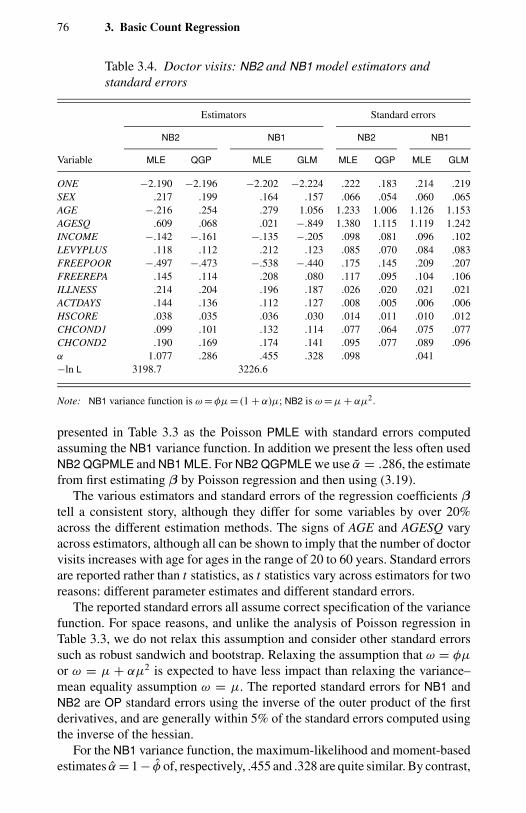
76 3. Basic Count Regression

Table 3.4. Doctor visits: NB2 and NB1 model estimators andstandard errors

Estimators Standard errors

NB2 NB1 NB2 NB1

Variable MLE QGP MLE GLM MLE QGP MLE GLM

ONE −2.190 −2.196 −2.202 −2.224 .222 .183 .214 .219SEX .217 .199 .164 .157 .066 .054 .060 .065AGE −.216 .254 .279 1.056 1.233 1.006 1.126 1.153AGESQ .609 .068 .021 −.849 1.380 1.115 1.119 1.242INCOME −.142 −.161 −.135 −.205 .098 .081 .096 .102LEVYPLUS .118 .112 .212 .123 .085 .070 .084 .083FREEPOOR −.497 −.473 −.538 −.440 .175 .145 .209 .207FREEREPA .145 .114 .208 .080 .117 .095 .104 .106ILLNESS .214 .204 .196 .187 .026 .020 .021 .021ACTDAYS .144 .136 .112 .127 .008 .005 .006 .006HSCORE .038 .035 .036 .030 .014 .011 .010 .012CHCOND1 .099 .101 .132 .114 .077 .064 .075 .077CHCOND2 .190 .169 .174 .141 .095 .077 .089 .096α 1.077 .286 .455 .328 .098 .041−ln L 3198.7 3226.6

Note: NB1 variance function is ω = φµ = (1 + α)µ; NB2 is ω = µ + αµ2.

presented in Table 3.3 as the Poisson PMLE with standard errors computedassuming the NB1 variance function. In addition we present the less often usedNB2 QGPMLE and NB1 MLE. For NB2 QGPMLE we use α = .286, the estimatefrom first estimating β by Poisson regression and then using (3.19).

The various estimators and standard errors of the regression coefficients βtell a consistent story, although they differ for some variables by over 20%across the different estimation methods. The signs of AGE and AGESQ varyacross estimators, although all can be shown to imply that the number of doctorvisits increases with age for ages in the range of 20 to 60 years. Standard errorsare reported rather than t statistics, as t statistics vary across estimators for tworeasons: different parameter estimates and different standard errors.

The reported standard errors all assume correct specification of the variancefunction. For space reasons, and unlike the analysis of Poisson regression inTable 3.3, we do not relax this assumption and consider other standard errorssuch as robust sandwich and bootstrap. Relaxing the assumption that ω = φµ

or ω = µ + αµ2 is expected to have less impact than relaxing the variance–mean equality assumption ω = µ. The reported standard errors for NB1 andNB2 are OP standard errors using the inverse of the outer product of the firstderivatives, and are generally within 5% of the standard errors computed usingthe inverse of the hessian.

For the NB1 variance function, the maximum-likelihood and moment-basedestimates α = 1 − φ of, respectively, .455 and .328 are quite similar. By contrast,

3.4. Overdispersion Tests 77

for the NB2 variance function the maximum-likelihood and moment-basedestimates α, respectively, 1.077 and .286, are quite different. The moment-based estimates for NB1 and NB2 use, respectively, (3.17) and (3.19). Anothermoment-based method, that given in Cameron and Trivedi (1986, p. 46), yieldsfor NB1 and NB2 variance functions estimates of, respectively, .218 and .490.Such differences in estimates of α have received little attention in the literature,in part because interest lies in estimation of β, with α a nuisance parameter.But even then they are important, as the standard error estimates of β dependon α.

Within the maximum likelihood framework the NB2 model is preferred hereto NB1 as it has higher log-likelihood, −3198.7 > −3226.6, with the same num-ber of parameters. In practice, most studies use either NB2 MLE or NB1 GLM.

3.4 Overdispersion Tests

Failure of the Poisson assumption of equidispersion has similar qualitativeconsequences to failure of the assumption of homoskedasticity in the linear re-gression model. But the magnitude of the effect on reported standard errors andt statistics can be much larger. To see this suppose ωi = 4µi . Then by equation(3.16) the variance matrix of the Poisson PML estimator is four times reportedmaximum likelihood standard errors using (3.6). As a result the reported Poissonmaximum likelihood t statistics need to be deflated by a factor of two. Overdis-persion as large as ωi = 4µi arises, for example, in the recreational trips data(see section 1.3) and in health services data on length of hospitalization.

Data are overdispersed if the conditional variance exceeds the conditionalmean. An indication of the magnitude of overdispersion or underdispersion canbe obtained simply by comparing the sample mean and variance of the depen-dent count variable. Subsequent Poisson regression decreases the conditionalvariance of the dependent variable somewhat. The average of the conditionalmean will be unchanged, however, as the average of the fitted means equalsthe sample mean. This follows because Poisson residuals sum to zero if a con-stant term is included. If the sample variance is less than the sample mean, thedata necessarily are even more underdispersed once regressors are included. Ifthe sample variance is more than twice the sample mean, then data are likelyto remain overdispersed after inclusion of regressors. This is particularly sofor cross-section data, for which regressors usually explain less than half thevariation in the data.

The standard models for overdispersion have already been presented. Theseare the NB1 variance function ωi = µi + αµi as in (3.11) or NB2 variancefunction ωi = µi +αµ2

i as in (3.13). If one takes the partially parametric mean–variance approach (GLM) it is much easier to use the NB1 variance function.If one takes the fully parametric negative binomial approach it is customary touse NB2. Note that if α = 0 the negative binomial reduces to the Poisson.

A sound practice is to estimate both Poisson and negative binomial modelsif software is readily available. The Poisson is the special case of the negative

78 3. Basic Count Regression

binomial with α = 0. The null hypothesis H0 : α = 0 can be tested against thealternative α > 0 using the hypothesis test methods presented in section 2.6.1.An LR test uses −2 times the difference in the fitted log-likelihoods of thetwo models. Alternatively a Wald test can by performed, using the reported tstatistic for the estimated α in the negative binomial model.

The distribution of these statistics is nonstandard, due to the restriction thatα cannot be less than zero. This complication is usually not commented on, anotable exception being Lawless (1987b). One way to see problems that ariseis to consider constructing a Monte Carlo experiment to obtain the distributionof the test statistic. We would draw samples from the Poisson, because thisis the model under the null hypothesis of no overdispersion. Roughly half thetime the data will be underdispersed. Then the negative binomial MLE for α iszero, the negative binomial parameter estimates equal the Poisson estimates,and the LR test statistic takes a value of 0. Clearly this test statistic is not χ2

distributed, because half its mass is at zero. Similar problems arise for the Waldtest statistic. A general treatment of hypothesis testing at boundary values isgiven by Moran (1971). The asymptotic distribution of the LR test statistic hasprobability mass of one half at zero and a half-χ2(1) distribution above 0. Thismeans that if testing at level δ, where δ > 0.5, one rejects H0 if the test statisticexceeds χ2

1−2δ(1) rather than χ21−δ(1). The Wald test is usually implemented as a

t test statistic, which here has mass of one half at zero and a normal distributionfor values above zero. In this case one continues to use the usual one-sided testcritical value of z1−δ . Essentially the only adjustment that needs to be madeis an obvious one to the χ2 critical values, which arises due to performing aone-sided rather than two-sided test.

If a package program for negative binomial regression is unavailable, one canstill test for overdispersion by estimating the Poisson model, constructing fittedvalues µi = exp(x′

i β), and performing the auxiliary OLS regression (withoutconstant)

(yi − µi )2 − yi

µi= αµi + ui , (3.39)

where ui is an error term. The reported t statistic for α is asymptotically nor-mal under the null hypothesis of no overdispersion against the alternative ofoverdispersion of the NB2 form. To test overdispersion of the NB1 form, replace(3.39) with

(yi − µi )2 − yi

µi= α + ui . (3.40)

These auxiliary regression tests coincide with the score or LM test for Poissonagainst negative binomial but additionally test for underdispersion and can begiven a more general motivation based on using only the specified mean andvariance (see Chapter 5).

Beyond rejection or nonrejection of the null hypothesis of equidispersion,interest may lie in interpreting the magnitude of departures from equidispersion.

3.5. Use of Regression Results 79

Estimates of α for the NB1 variance function (1 + α)µi are easily interpreted,with underdispersion if α < 0, modest overdispersion when, say, 0 < α < 1,and considerable overdispersion if, say, α > 1. For the NB2 variance functionµi + αµ2

i underdispersion also occurs if α < 0. The NB2 variance functioncan be inappropriate for underdispersed data, as the estimated variance is neg-ative for observations with α < − 1/µi . For interpretation of the magnitude ofoverdispersion it is helpful to rewrite the NB2 variance as (1 + αµi ) µi . Thenvalues of considerable overdispersion arise if, say, αµi > 1, because then themultiplier 1 + αµi > 2. Thus a value of α equal to 0.5 would indicate modestoverdispersion if the dependent variable took mostly values of 0, 1 and 2, butgreat overdispersion if counts of 10 or more were often observed.

Most often count data are overdispersed rather than underdispersed, and testsfor departures from equidispersion are usually called overdispersion tests. Notethat the negative binomial model can only accommodate overdispersion.

Example: Doctor Visits (Continued)

From Table 3.1 the data before inclusion of regressors are overdispersed, withvariance–mean ratio of .637/.302 = 2.11. The only question is whether thisoverdispersion disappears on inclusion of regressors.

We first consider tests of Poisson against NB2 at significance level 1%. Giventhe results in Tables 3.3 and 3.4 the LR test statistic is 2(3355.5 − 3198.7) =313.6, which exceeds the 1% critical value of χ2

.98(1) = 5.41. The Wald teststatistic from Table 3.4 is 1.077/.098 = 10.99, which exceeds the 1% criticalvalue of z.99 = 2.33. Finally, the LM test statistic computed using the auxil-iary regression (3.39) is 7.51, and exceeds the 1% critical value of z.99 = 2.33.Therefore all three tests strongly reject the null hypothesis of Poisson, indicatingthe presence of overdispersion. Note that these tests are asymptotically equiva-lent, yet there is quite a difference in their realized values of

√313.6 = 17.69,

10.9, and 7.51.Similar test statistics for Poisson against NB1 are TLR = 2 × (3355.5 −

3226.6) = 257.8, TW = .455/.041 = 11.10 and TLM = 6.543 on running auxil-iary regression (3.40). These again strongly reject equidispersion.

Clearly some control is necessary for overdispersion. Possibilities includethe Poisson PML, see Table 3.3, which corrects the standard errors for overdis-persion, and the various NB1 and NB2 estimators presented in Table 3.4.

3.5 Use of Regression Results

The techniques presented to date allow estimation of count data models andperformance of tests of statistical significance of regression coefficients. Wehave focused on tests on individual coefficients. Tests of joint hypotheses suchas overall significance can be performed using the Wald, LM, and LR testspresented in section 2.6.1. Confidence intervals for functions of parameters canbe formed using the delta method in section 2.6.2.

80 3. Basic Count Regression

We now turn to interpretation of regression coefficients and prediction of thedependent variable.

3.5.1 Interpretation of Coefficients

An important issue is interpretation of regression coefficients. For example,what does β j = 0.2 mean? This is straightforward in the linear regression modelE[y | x] = x′β. Then ∂E[y | x]/∂x j = β j , so β j = 0.2 means that a one-unitchange in the j th regressor increases the conditional mean by 0.2 units.

We consider the exponential conditional mean

E[y | x] = exp(x′β), (3.41)

where for exposition the subscript i is dropped. Let the scalar x j denote the j th

regressor. Differentiating

∂E[y | x]

∂x j= β j exp

(x′

iβ). (3.42)

For example, if β j = 0.2 and exp(x′i β) = 2.5, then a one-unit change in the

j th regressor increases the expectation of y by 0.5 units.Calculated values differ across individuals, however, due to different values

of x. This makes interpretation more difficult.One procedure is to aggregate over all individuals and calculate the average

response

1

n

n∑i=1

∂E[yi | xi ]

∂xi j= 1

n

n∑i=1

β j exp(x′

iβ). (3.43)

In the special case that one uses the Poisson MLE or PMLE, and the regressionincludes an intercept term, this expression simplifies to

1

n

n∑i=1

∂E[yi | xi ]

∂xi j= β j y (3.44)

because the first-order conditions imply∑

i exp(x′iβ) =∑i yi .

A second procedure is to calculate the response for the individual withaverage characteristics

∂E[y | x]

∂x j

∣∣∣∣x

= β j exp(x′β). (3.45)

Because exp(·) is a convex function, by Jensen’s inequality the average of exp(·)evaluated at several points exceeds exp(·) evaluated at the average of the samepoints. So (3.45) gives responses smaller than (3.43). Due to the need for lesscalculation, it is common in nonlinear regression to report responses at the

3.5. Use of Regression Results 81

sample mean of regressors. It is conceptually better, however, to report theaverage response (3.43) over all individuals. And it is actually easier in thespecial case of Poisson with intercept included, as (3.44) can be used.

A third procedure is to calculate (3.42) for select values of x j of particularinterest. This is perhaps the best method. The actual values of x j of particularinterest vary from application to application.

It is useful to note that direct interpretation of the coefficients is possiblewithout such additional computations.

• The coefficient β j equals the proportionate change in the conditionalmean if the j th regressor changes by one unit. This follows from rewrit-ing (3.42) as ∂E[y | x]/∂x j = β j E[y | x], using (3.41), and hence

β j = ∂E[y | x]

∂x j

1

E[y | x]. (3.46)

This is a semielasticity, which can alternatively be obtained by rewrit-ing (3.41) as ln E[y | x] = x′β and differentiating with respect to x j .

• The sign of the response ∂E[y | x]/∂x j is given by the sign of β j ,because the response is β j times the scalar exp (x′

iβ), which is alwayspositive.

• If one regression coefficient is twice as large as another, then the effectof a one-unit change of the associated regressor is double that of theother. This result follows from

∂E[y | x]/∂x j

∂E[y | x]/∂xk= β j exp(x′β)

βk exp(x′β)= β j

βk. (3.47)

A single-index model is one for which E[y | x] = g(x′β), for monotonicfunction g(·). The last two properties hold more generally for any single-indexmodel.

Sometimes regressors enter logarithmically in (3.41). For example, we mayhave

E[y | x] = exp(β1 ln(x1) + x′

2β2)

= xβ11 exp

(x′

2β2).

Then β1 is an elasticity, giving the percentage change in E[y | x] for a 1% changein x1. This formulation is particularly appropriate if x1 is a measure of exposure,such as number of miles driven if modeling the number of automobile accidentsor population if modeling the incidence of a disease. Then we expect β1 to beclose to unity.

The conditional mean function may include interaction terms. For example,suppose

E[y | x] = exp(β1 + β2x2 + β2x3 + β4x2x3).

82 3. Basic Count Regression

Then the proportionate change in the conditional mean due to a one-unit changein x3 equals (β2 + β4x2), because

∂E[y | x]

∂x3

1

E[y | x]= (β2 + β4x2).

Thus even the semielasticity measuring the effect of changes in x3 varies ac-cording to the value of regressors – here x2.

The calculus methods above are appropriate for continuous regressors. Nowconsider an indicator variable regressor d that takes only values 0 and 1, andsuppose

E[y | d, x2] = exp(β1d + x′

2β2).

Then

E[y | d = 1, x2]

E[y | d = 0, x2]= exp

(β1 + x′

2β2)

exp(x′

2β2) = exp(β1).

So the conditional mean is exp(β1) times larger if the indicator variable isunity rather than zero. If we instead use calculus methods then (3.46) predicts aproportionate change of β1, or equivalently that the conditional mean is (1+β1)times larger. This is a good approximation for small β1, say β1 < 0.1, as thenexp(β1) 1 + β1.

The preceding discussion has considered the effect of a one-unit change inx, which is not free of the units used to measure x. One method is to scale by thesample mean of x j , so use β j x j , which given (3.42) is a measure of the elasticityof E[y | x] with respect to x j . An alternative method is to consider semistan-dardized coefficients that give the effect of a one-standard-deviation change inx j , so use β j s j , where s j is the standard deviation of x j . Such adjustments, ofcourse, need to be made even for the linear regression model.

Example: Doctor Visits (Continued)

Various measures of the magnitude of the response of the number of doctorvisits to changes in regressors are given in Table 3.5. These measures are basedon the Poisson PMLE estimates given earlier in Table 3.3.

The coefficient estimates given in the column labeled PMLE using (3.46)can be interpreted as giving the proportionate change in number of doctor visitsdue to a one-unit change in the regressors. If we consider ACTDAYS, the mosthighly statistically significant regressor, an increase of 1 day of reduced activityin the preceding 2 weeks leads to a .127 proportionate change or 12.7% changein the expected number of doctor visits. More complicated is the effect of age,which appears through both AGE and AGESQ. For a 40-year-old person, AGE= .4 and AGESQ = .16, and an increase of 1 year or 0.01 units leads to a0.01× (1.056−2× .849× .40) = .0038 proportionate change or .38% changein the expected number of doctor visits.

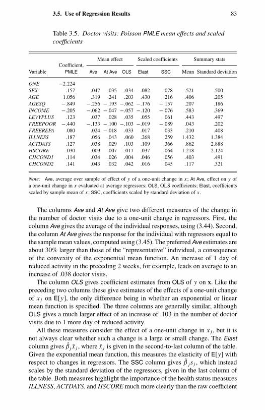
3.5. Use of Regression Results 83

Table 3.5. Doctor visits: Poisson PMLE mean effects and scaledcoefficients

Mean effect Scaled coefficients Summary statsCoefficient,

Variable PMLE Ave At Ave OLS Elast SSC Mean Standard deviation

ONE −2.224SEX .157 .047 .035 .034 .082 .078 .521 .500AGE 1.056 .319 .241 .203 .430 .216 .406 .205AGESQ −.849 −.256 −.193 −.062 −.176 −.157 .207 .186INCOME −.205 −.062 −.047 −.057 −.120 −.076 .583 .369LEVYPLUS .123 .037 .028 .035 .055 .061 .443 .497FREEPOOR −.440 −.133 −.100 −.103 −.019 −.089 .043 .202FREEREPA .080 .024 −.018 .033 .017 .033 .210 .408ILLNESS .187 .056 .043 .060 .268 .259 1.432 1.384ACTDAYS .127 .038 .029 .103 .109 .366 .862 2.888HSCORE .030 .009 .007 .017 .037 .064 1.218 2.124CHCOND1 .114 .034 .026 .004 .046 .056 .403 .491CHCOND2 .141 .043 .032 .042 .016 .045 .117 .321

Note: Ave, average over sample of effect of y of a one-unit change in x ; At Ave, effect on y ofa one-unit change in x evaluated at average regressors; OLS, OLS coefficients; Elast, coefficientsscaled by sample mean of x ; SSC, coefficients scaled by standard deviation of x .

The columns Ave and At Ave give two different measures of the change inthe number of doctor visits due to a one-unit change in regressors. First, thecolumn Ave gives the average of the individual responses, using (3.44). Second,the column At Ave gives the response for the individual with regressors equal tothe sample mean values, computed using (3.45). The preferred Ave estimates areabout 30% larger than those of the “representative” individual, a consequenceof the convexity of the exponential mean function. An increase of 1 day ofreduced activity in the preceding 2 weeks, for example, leads on average to anincrease of .038 doctor visits.

The column OLS gives coefficient estimates from OLS of y on x. Like thepreceding two columns these give estimates of the effects of a one-unit changeof x j on E[y], the only difference being in whether an exponential or linearmean function is specified. The three columns are generally similar, althoughOLS gives a much larger effect of an increase of .103 in the number of doctorvisits due to 1 more day of reduced activity.

All these measures consider the effect of a one-unit change in x j , but it isnot always clear whether such a change is a large or small change. The Elastcolumn gives β j x j , where x j is given in the second-to-last column of the table.Given the exponential mean function, this measures the elasticity of E[y] withrespect to changes in regressors. The SSC column gives β j s j , which insteadscales by the standard deviation of the regressors, given in the last column ofthe table. Both measures highlight the importance of the health status measuresILLNESS, ACTDAYS, and HSCORE much more clearly than the raw coefficient

84 3. Basic Count Regression

estimates and the estimates of ∂E[y]/∂x j . For example, the estimates implythat a 1% increase in illness days leads to a .268% increase in expected doctorvisits, while a one-standard-deviation increase in activity days leads to a .259%increase in expected doctor visits.

3.5.2 Prediction

We begin by considering, for an individual observation with x = xp, predictionof the conditional mean µp = E[y | x = xp].

For the exponential conditional mean function, the mean prediction is

µp = exp(x′

pβ). (3.48)

A 95% confidence interval, which allows for the imprecision in the estimateβ, can be obtained using the delta method given in section 2.6.2. Considerestimation procedures that additionally estimate a scalar nuisance parameter α,to accommodate overdispersion. Because ∂µp/∂β = µpxp and ∂µp/∂α = 0,we obtain

µp ∈ µp ± z.025

õ2

px′pV[β]xp, (3.49)

for estimator βa∼ N[β, V[β]]. As expected, greater precision in the estimation

of β leads to a narrower confidence interval.One may also wish to predict the actual value of y, rather than its predicted

mean. This is considerably more difficult, as the randomness of y needs tobe accounted for, in addition to the randomness in the estimator β. For lowcounts in particular, individual values are poorly predicted due to the intrinsicrandomness of y.

For an individual observation with x = xp, and using the exponential con-ditional mean function, the individual prediction is

yp = exp(x′

pβ). (3.50)

Note that while y p equals µp, it is being used as an estimate of yp rather than µp.If we consider variance functions of the form (3.9), the estimated variance of yp

is ω(µp, α). Adding this to the earlier variance due to imprecision in the estimateβ, the variance of y p is consistently estimated by ω(µp, α) + µ2

px′pV[β]xp. A

two-standard error interval is

yp ∈ y p ± 2√

ω(µp, α) + µ2px′

pV[β]xp. (3.51)

This can be used as a guide but is not formally a 95% confidence intervalbecause yp is not normally distributed even in large samples.

The width of this interval is increasing in µp, because ω(µp, α) is increasingin µp. The interval is quite wide, even for low counts. For example, consider thePoisson distribution, so ω(µ, α) = µ, and assume a large sample size, so that βis very precisely estimated and V[β] 0. Then (3.51) becomes yp ∈ y p±2

√y p.

3.6. Ordered and Other Discrete-Choice Models 85

Even for y p = 4 this yields (0, 8). If y is Poisson and β is known it is better todirectly use this knowledge, rather than the approximation (3.51). Then becausePr [1 ≤ yp ≤ 8] = .0397 when yp is Poisson-distributed with µp = 4, a 96.03%confidence interval for yp is (1,8).

Interest can also lie in predicting the probabilities of particular values of yoccurring, for an individual observation with x = xp. Let pk denote the proba-bility that yp = k if x = xp. For the Poisson, for example, this is estimated bypk = exp(−µp)µk

p/k!, where µp is given in (3.48). The delta method can beused to obtain a confidence interval for pk . Most parametric models include anoverdispersion parameter α. Because ∂pk/∂α = 0 the delta method does notyield an interval as simple as (3.49).

A fourth quantity that might be predicted is the change in the conditionalmean if the j th regressor changes by one unit. From (3.42) the predicted changeis β j µp. Again the delta method can be used to form a confidence interval.

As the sample size gets very large the variance of β goes to zero and the confi-dence intervals for predictions of the conditional mean, individual probabilities,and changes in predicted probabilities collapse to a point. The confidence in-tervals for predictions of individual values of y, however, can remain wideas demonstrated above. Thus, within-sample individual predictions of y differconsiderably from the actual values of y, especially for small counts. If interestis in assessing the usefulness of model predictions, it can be better to considerpredictions at a more aggregated level. This is considered in Chapter 5.

The preceding methods require use of a computer program that saves thevariance matrix of the regression parameters and permits matrix multiplication.It is generally no more difficult to instead use the bootstrap, which has the addi-tional advantages of providing asymmetric confidence intervals and potentiallybetter small-sample performance.

More problematic in practice is deciding what values of xp to use in pre-diction. If, for example, there are just two regressors, both binary, one wouldsimply predict for each of the four distinct values of x. But in practice there aremany different distinct values of x, and it may not be obvious which few valuesto focus on. Such considerations also arise in the linear regression model.

3.6 Ordered and Other Discrete-Choice Models

Count data can alternatively be modeled using discrete choice methods surveyedin Maddala (1983). This is particularly natural if most observed counts takevalues 0 and 1, with few counts in excess of 1. Then one might simply modelwhether the count is zero or nonzero, using a binary choice model such as logitor probit. This leads, however, to a loss of precision in estimation.

Now suppose most observed counts take values 0, 1, or 2, with few countsin excess of 2. For data with three choices, in this case 0, 1, and 2 or more,the standard discrete choice model is the multinomial logit model, but this hasdeficiencies given subsequently here. It is better to use an ordered model, suchas ordered probit or ordered logit.

86 3. Basic Count Regression

Ordered discrete-choice models treat the data as generated by a continuousunobserved latent variable, which on crossing a threshold leads to an increaseof one in the observed number of events. This is a representation of the dgpquite different from the Poisson process, which leads to the Poisson density forcounts. In theory, one should use an ordered model for data for which the dgpis felt to be a continuous latent variable. In practice, ordered models have beenrarely applied to count data outside the cross-section setting.

3.6.1 Binary-Choice Models

Let yi be the count variable of interest. Define the indicator variable

di = 1 if yi > 0

= 0 if yi = 0.(3.52)

This equals the count variable except that yi values of 2 or more are recoded to1. Other partitions are possible, such as yi > k and yi ≤ k.

The general form of such a binary choice model is

Pr[di = 1] = F(x′

iβ)

Pr[di = 0] = 1 − F(x′

iβ),

(3.53)

where 0 < F(·) < 1. It is customary to let the probability be a transformation ofa linear combination of the regressors rather than use the more general functionalform F(xi ,β). By construction the probabilities sum to one. A parsimoniousway to write the density given by (3.53) is F(x′

iβ)di (1 − F(x′iβ))1−di , which

leads to the log-likelihood function

ln L =n∑

i = 1

di ln F(x′

iβ)+ (1 − di ) ln

(1 − F

(x′

iβ))

. (3.54)

Different binary choice models correspond to different choice of the functionF(·). Standard choices include the logit model, which corresponds to F(z) =exp(z)/(1 + exp(z)); and the probit model, which corresponds to F(z) = (z)where (·) is the standard normal cdf.

There is a loss of efficiency due to combining all counts in excess of zerointo a single category. Suppose yi are Poisson distributed with mean µi . ThenPr[di = 1] = Pr [yi > 0] = 1 − exp(−µi ), so for µi = exp(x′

iβ).

F(x′

iβ)= 1 − exp

(−exp(x′

iβ))

.

The binary Poisson MLE βBP maximizes (3.54) with this choice of F(·). It canbe shown that

V[βBP] =(

n∑i = 1

ciµi xi x′i

)−1

,

3.6. Ordered and Other Discrete-Choice Models 87

where ci = µi exp(−µi )/(1 − exp(−µi )). V[βBP] exceeds (∑n

i = 1 µi xi x′i )

−1,the variance matrix of the Poisson MLE from (3.6), because ci < 1 for µi > 0.

As expected, the relevant efficiency loss is increasing in the Poisson mean.For example, for µi = .5 and 1, respectively, ci = .77 and .58. In the Poissoniid case with µ = .5, the standard error of βBP is

√1/.77 = 1.14 times that of

the Poisson MLE, even though less than 10% of the counts will exceed unity.

3.6.2 Ordered Probit

The Poisson and negative binomial models treat discrete data as being theresult of an underlying point process. One could instead model the numberof doctor visits, for example, as being due to a continuous process that oncrossing a threshold leads to a visit to a doctor. Crossing further thresholdsleads to additional doctor visits. Before specializing to threshold models suchas ordered probit, we first present general results for multinomial models.

Suppose the count variable yi takes values 0, 1, 2, . . . , m. Define the m + 1indicator variables

di j = 1 yi =, j

= 0 yi = j.(3.55)

Also define the corresponding probabilities

Pr[di j = 1] = pi j , j = 0, . . . , m, (3.56)

where pi j may depend on regressors and parameters. Then the density functionfor the i th observation can be written as

f (yi ) = f (di0, di1, . . . , dim) =m∏

j = 0

pdi j

i j , (3.57)

and the log-likelihood function is

ln L =n∑

i = 1

m∑j = 0

di j ln pi j . (3.58)

Different multinomial models arise from different specification of the prob-abilities pi j . The most common is the multinomial logit model, which specifiespi j = exp(x′

iβ j )/ (∑m

k = 0 x′iβk) in (3.58). This model is inappropriate for count

data for which the outcome, the number of occurrences of an event, is naturallyordered. One way to see this is to note that a property of multinomial logit isthat the relative probabilities of any two outcomes are independent of the prob-abilities of other outcomes. For example, the probability of one doctor visit,conditional on the probability of zero or one visit, would not depend on theprobability of two visits. But one expects that this conditional probability willbe higher the higher the probability of two visits. It is better to use a multinomialmodel that explicitly incorporates the ordering of the data.

88 3. Basic Count Regression

The ordered probit model, presented for example in Maddala (1983), intro-duces a latent (unobserved) random variable

y∗i = x′

iβ + εi , (3.59)

where εi is N[0, 1]. The observed discrete data variable yi is generated fromthe unobserved y∗

i in the following way:

yi = j if α j < y∗i ≤ α j+1, j = 0, . . . , m, (3.60)

where α0 = −∞ and αm+1 = ∞. It follows that

pi j = Pr[α j < y∗

i ≤ α j+1]

= Pr[α j − x′

iβ < εi ≤ α j+1 − x′iβ]

= (α j+1 − x′

iβ)−

(α j − x′

iβ), (3.61)

where (·) is the standard normal cdf, j = 0, 1, 2, . . . , m, and αm+1 = ∞. Thelog-likelihood function (3.58) with probabilities (3.61) is

ln L =n∑

i = 1

m∑j = 0

di j ln[(α j+1 − x′

iβ)−

(α j − x′

iβ)]

. (3.62)

Estimation of β and α1, . . . , αm by maximum likelihood is straightforward.Identification requires a normalization, such as 0, for one of α1, . . . , αm or theintercept term in β.

If there are many counts or few observations for a given count then someaggregation of count data may be necessary. For example, if there are fewobservations larger than three one might have categories of 0, 1, 2, and 3 ormore. As an alternative to the ordered probit one can use the ordered logitmodel, in which case (·) is replaced by the logistic cdf L(z) = ez/(1 + ez).More generally if εi in (3.59) has a nonnormal distribution the log-likelihoodfunction is (3.62) with (·) replaced by the cdf of εi .

The ordered discrete choice model has the additional attraction of beingapplicable to count data that are negative. Such data may arise if instead ofdirectly modeling a count variable, one differences and models the change inthe count. For example, some U.S. stock prices are a count, as they are measuredin units of a tick, or one eighth of a dollar. Hausman, Lo, and MacKinlay (1992)modeled price changes in consecutive time-stamped trades of a given stockusing the ordered probit model, generalized to allow εi to be N[0, σ 2

i ] wherethe variance σ 2

i is itself modeled by a regression equation.

3.7 Other Models

In this section we consider whether least-squares methods might be usefullyapplied to count data y. Three variations of least squares are considered. Thefirst is linear regression of y on x, making no allowance for the count nature

3.7. Other Models 89

of the data aside from using heteroskedasticity robust standard errors. The sec-ond is linear regression of a nonlinear transformation of y on x, for whichthe transformation leads to a dependent variable that is close to homoskedas-tic and symmetric. Third, we consider nonlinear least squares regression withconditional mean of y specified to be exp(x′β).

The section finishes with a discussion of estimation using duration data,rather than count data, if the data are generated by a Poisson process.

3.7.1 OLS without Transformation

The OLS estimator is clearly inappropriate as it specifies a conditional meanfunction x′γ that may take negative values and a variance function that ishomoskedastic. If the conditional mean function is in fact exp(x′β), the OLSestimator is inconsistent for β and the computed OLS output gives the wrongasymptotic variance matrix.

Nonetheless, OLS estimates in practice give results qualitatively similar tothose for Poisson and other estimators using the exponential mean. The ratioof OLS slope coefficients is often similar to the ratio of Poisson slope coeffi-cients, with the OLS slope coefficients approximately y times the Poisson slopecoefficients, and the most highly statistically significant regressors from OLSregression, using usual OLS output t statistics, are in practice the most highlysignificant using Poisson regression. This is similar to comparing different mod-els for binary data such as logit, probit, and OLS. In all cases the conditionalmean is restricted to be of form g(x′β), which is a monotonic transformationof a linear combination of the regressors. The only difference across models isthe choice of function g, which leads to a different scaling of the parameters β.

A first-order Taylor series expansion of the exponential mean exp(x′β)around the sample mean y, that is, around x′β= ln y, yields exp(x′β) = y +y(x′β− ln y). For models with intercept, this can be rewritten as exp(β1 +x′

2β2) = γ1 + x′2γ2, where γ1 = y + β1 y − ln y and γ2 =β2 y. So linear mean

slope coefficients are approximately y times exponential slope coefficients. Thisapproximation will be more reasonable the less dispersed the predicted valuesexp(x′

i β) are about y.

The OLS estimator can be quite useful for preliminary data analysis, such asdetermining key variables, in simple count models. Dealing with more compli-cated count models for which no off-the-shelf software is readily available iseasier if one first ignores the count aspect of the data and does the correspondingadjustment to OLS. For example, if the complication is endogeneity, then dolinear two-stage least squares as a potential guide to the impact of endogeneity.But experience is sufficiently limited that one cannot advocate this approach.

3.7.2 OLS with Transformation

For skewed continuous data such as that on individual income or on housingprices a standard transformation is the log transformation. For example, if y is

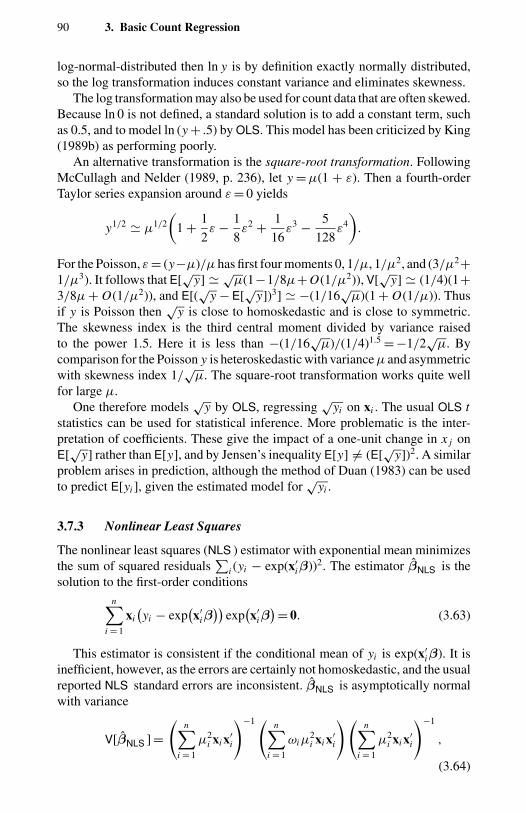
90 3. Basic Count Regression

log-normal-distributed then ln y is by definition exactly normally distributed,so the log transformation induces constant variance and eliminates skewness.

The log transformation may also be used for count data that are often skewed.Because ln 0 is not defined, a standard solution is to add a constant term, suchas 0.5, and to model ln (y + .5) by OLS. This model has been criticized by King(1989b) as performing poorly.

An alternative transformation is the square-root transformation. FollowingMcCullagh and Nelder (1989, p. 236), let y = µ(1 + ε). Then a fourth-orderTaylor series expansion around ε = 0 yields

y1/2 µ1/2

(1 + 1

2ε − 1

8ε2 + 1

16ε3 − 5

128ε4

).

For the Poisson, ε = (y−µ)/µ has first four moments 0, 1/µ, 1/µ2, and (3/µ2+1/µ3). It follows that E[

√y] √

µ(1−1/8µ+ O(1/µ2)), V[√

y] (1/4)(1+3/8µ + O(1/µ2)), and E[(

√y − E[

√y])3] −(1/16

√µ)(1 + O(1/µ)). Thus

if y is Poisson then√

y is close to homoskedastic and is close to symmetric.The skewness index is the third central moment divided by variance raisedto the power 1.5. Here it is less than −(1/16

√µ)/(1/4)1.5 = −1/2

õ. By

comparison for the Poisson y is heteroskedastic with variance µ and asymmetricwith skewness index 1/

õ. The square-root transformation works quite well

for large µ.One therefore models

√y by OLS, regressing

√yi on xi . The usual OLS t

statistics can be used for statistical inference. More problematic is the inter-pretation of coefficients. These give the impact of a one-unit change in x j onE[

√y] rather than E[y], and by Jensen’s inequality E[y] = (E[

√y])2. A similar

problem arises in prediction, although the method of Duan (1983) can be usedto predict E[yi ], given the estimated model for

√yi .

3.7.3 Nonlinear Least Squares

The nonlinear least squares (NLS ) estimator with exponential mean minimizesthe sum of squared residuals

∑i (yi − exp(x′

iβ))2. The estimator βNLS is thesolution to the first-order conditions

n∑i = 1

xi(yi − exp

(x′

iβ))

exp(x′

iβ)= 0. (3.63)

This estimator is consistent if the conditional mean of yi is exp(x′iβ). It is

inefficient, however, as the errors are certainly not homoskedastic, and the usualreported NLS standard errors are inconsistent. βNLS is asymptotically normalwith variance

V[βNLS ] =(

n∑i = 1

µ2i xi x′

i

)−1 ( n∑i = 1

ωiµ2i xi x′

i

)(n∑

i = 1

µ2i xi x′

i

)−1

,

(3.64)

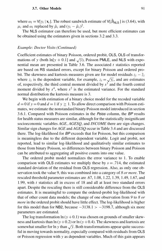
3.7. Other Models 91

where ωi = V[yi | xi ]. The robust sandwich estimate of V[βNLS ] is (3.64), withµi and ωi replaced by µi and (yi − µi )2.

The NLS estimator can therefore be used, but more efficient estimates canbe obtained using the estimators given in sections 3.2 and 3.3.

Example: Doctor Visits (Continued)

Coefficient estimates of binary Poisson, ordered probit, OLS, OLS of transfor-mations of y (both ln[y + 0.1] and

√y), Poisson PMLE, and NLS with expo-

nential mean are presented in Table 3.6. The associated t statistics reportedare based on RS standard errors, except for binary Poisson and ordered pro-bit. The skewness and kurtosis measures given are for model residuals zi − zi

where zi is the dependent variable, for example, zi = √yi , and are estimates

of, respectively, the third central moment divided by s3 and the fourth centralmoment divided by s4, where s2 is the estimated variance. For the standardnormal distribution the kurtosis measure is 3.

We begin with estimation of a binary choice model for the recoded variabled = 0 if y = 0 and d = 1 if y ≥ 1. To allow direct comparison with Poisson esti-mates, we estimate the nonstandard binary Poisson model introduced in section3.6.1. Compared with Poisson estimates in the Poiss column, the BP resultsfor health status measures are similar, although for the statistically insignificantsocioeconomic variables AGE, AGESQ, and INCOME there are sign changes.Similar sign changes for AGE and AGESQ occur in Table 3.4 and are discussedthere. The log-likelihood for BP exceeds that for Poisson, but this comparisonis meaningless due to the different dependent variable. Logit and probit, notreported, lead to similar log-likelihood and qualitatively similar estimates tothose from binary Poisson, so differences between binary Poisson and Poissoncan be attributed to aggregating all positive counts into one value.

The ordered probit model normalizes the error variance to 1. To enablecomparison with OLS estimates we multiply these by s = .714, the estimatedstandard deviation of the residual from OLS regression. Also, as only one ob-servation took the value 9, this was combined into a category of 8 or more. Therescaled threshold parameter estimates are .67, 1.08, 1.22, 1.39, 1.49, 1.67, and1.99, with t statistics all in excess of 18 and all at least two standard errorsapart. Despite the rescaling there is still considerable difference from the OLSestimates. It is meaningful to compare the ordered-probit log-likelihood withthat of other count data models; the change of one observation from 9 to 8 ormore in the ordered probit should have little effect. The log-likelihood is higherfor this model than for NB2, because −3138.1 > −3198.7, although six moreparameters are estimated.

The log transformation ln (y +0.1) was chosen on grounds of smaller skew-ness and kurtosis than ln (y +0.2) or ln (y +0.4). The skewness and kurtosis aresomewhat smaller for ln y than

√y. Both transformations appear quite success-

ful in moving towards normality, especially compared with residuals from OLSor Poisson regression with y as dependent variables. Much of this gain appears

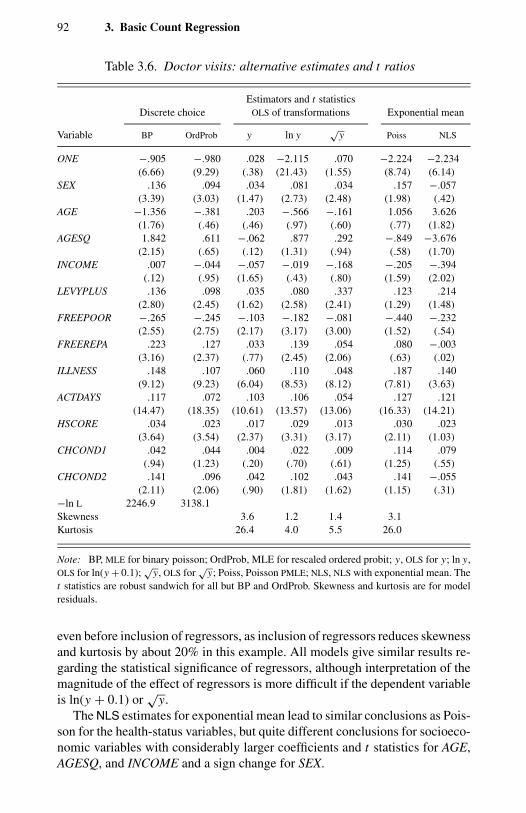
92 3. Basic Count Regression

Table 3.6. Doctor visits: alternative estimates and t ratios

Estimators and t statisticsDiscrete choice OLS of transformations Exponential mean

Variable BP OrdProb y ln y√

y Poiss NLS

ONE −.905 −.980 .028 −2.115 .070 −2.224 −2.234(6.66) (9.29) (.38) (21.43) (1.55) (8.74) (6.14)

SEX .136 .094 .034 .081 .034 .157 −.057(3.39) (3.03) (1.47) (2.73) (2.48) (1.98) (.42)

AGE −1.356 −.381 .203 −.566 −.161 1.056 3.626(1.76) (.46) (.46) (.97) (.60) (.77) (1.82)

AGESQ 1.842 .611 −.062 .877 .292 −.849 −3.676(2.15) (.65) (.12) (1.31) (.94) (.58) (1.70)

INCOME .007 −.044 −.057 −.019 −.168 −.205 −.394(.12) (.95) (1.65) (.43) (.80) (1.59) (2.02)

LEVYPLUS .136 .098 .035 .080 .337 .123 .214(2.80) (2.45) (1.62) (2.58) (2.41) (1.29) (1.48)

FREEPOOR −.265 −.245 −.103 −.182 −.081 −.440 −.232(2.55) (2.75) (2.17) (3.17) (3.00) (1.52) (.54)

FREEREPA .223 .127 .033 .139 .054 .080 −.003(3.16) (2.37) (.77) (2.45) (2.06) (.63) (.02)

ILLNESS .148 .107 .060 .110 .048 .187 .140(9.12) (9.23) (6.04) (8.53) (8.12) (7.81) (3.63)

ACTDAYS .117 .072 .103 .106 .054 .127 .121(14.47) (18.35) (10.61) (13.57) (13.06) (16.33) (14.21)

HSCORE .034 .023 .017 .029 .013 .030 .023(3.64) (3.54) (2.37) (3.31) (3.17) (2.11) (1.03)

CHCOND1 .042 .044 .004 .022 .009 .114 .079(.94) (1.23) (.20) (.70) (.61) (1.25) (.55)

CHCOND2 .141 .096 .042 .102 .043 .141 −.055(2.11) (2.06) (.90) (1.81) (1.62) (1.15) (.31)

−ln L 2246.9 3138.1Skewness 3.6 1.2 1.4 3.1Kurtosis 26.4 4.0 5.5 26.0

Note: BP, MLE for binary poisson; OrdProb, MLE for rescaled ordered probit; y, OLS for y; ln y,OLS for ln(y + 0.1);

√y, OLS for

√y; Poiss, Poisson PMLE; NLS, NLS with exponential mean. The

t statistics are robust sandwich for all but BP and OrdProb. Skewness and kurtosis are for modelresiduals.

even before inclusion of regressors, as inclusion of regressors reduces skewnessand kurtosis by about 20% in this example. All models give similar results re-garding the statistical significance of regressors, although interpretation of themagnitude of the effect of regressors is more difficult if the dependent variableis ln(y + 0.1) or

√y.

The NLS estimates for exponential mean lead to similar conclusions as Pois-son for the health-status variables, but quite different conclusions for socioeco-nomic variables with considerably larger coefficients and t statistics for AGE,AGESQ, and INCOME and a sign change for SEX.

3.8. Iteratively Reweighted Least Squares 93

3.7.4 Exponential Duration Model

For a Poisson point process the number of events in a given interval of timeis Poisson distributed. The duration of a spell, the time from one occurrenceto the next, is exponentially distributed. Here we consider modeling durationsrather than counts.

Suppose that for each individual in a sample of n individuals we observe theduration of one complete spell, generated by a Poisson point process with rateparameter γi . Then ti has exponential density f (ti ) = γi exp(−γi ti ) with meanE[ti ] = 1/γi . For regression analysis it is customary to specify γi = exp(x′

iβ).The exponential MLE, βE, maximizes the log-likelihood function

ln L =n∑

i = 1

x′iβ − exp

(x′

iβ)ti . (3.65)

The first-order conditions can be expressed as

n∑i = 1

(1 − exp

(x′

iβ)ti)xi = 0, (3.66)

and application of the usual maximum likelihood theory yields

VML[βE] =(

n∑i = 1

xi x′i

)−1

. (3.67)

If instead we modeled the number of events from a Poisson point processwith rate parameter γi = exp(x′

iβ) we obtain

VML[βP] =(

n∑i = 1

γi xi x′i

)−1

.

The two variance matrices coincide if γi = 1. Thus if we choose intervalsfor each individual so that individuals on average experience one event suchas a doctor visit, the count data have the same information content, in terms ofprecision of estimation of β, as observing for each individual one completedspell such as time between successive visits to the doctor. More simply, onecount conveys the same information as the length of one complete spell.

3.8 Iteratively Reweighted Least Squares

Most of the models and estimators in this book require special statistical pack-ages for nonlinear models. An exception is the Poisson PMLE, which can becomputed in the following way.

In general at the sth iteration, the Newton-Raphson method updates the cur-rent estimate βs by the formula βs+1 = βs − H−1

s gs , where g = ∂ ln L/∂β and

94 3. Basic Count Regression

H = ∂2 ln L/∂β∂β′ are evaluated at βs . Here this becomes

βs+1 = βs +[

n∑i = 1

µisxi x′i

]−1 n∑i = 1

xi (yi − µis),

where we consider the exponential mean function so µis = exp(x′i βs). This can

be rewritten as

βs+1 =[

n∑i = 1

(õisxi

)(õisxi

)′]−1 n∑i = 1

(õisxi

)√

µis(yi − µis)

µis+√

µisx′i βs

,

which is the formula for the OLS estimator from the regressionõis

(yi − µis)

µis+ x′

i βs

= (õisxi

)′βs+1 + ui , (3.68)

where ui is an error term. Thus the Poisson PMLE can be calculated by thisiterative OLS regression. Equivalently, it can be estimated by WLS regressionof ((yi − µis)/µis) + x′

i βs on xi , where the weights√

µis change at eachiteration.

For the general conditional mean function µi = µ(xi ,β), the method of scor-ing, which replaces H by E[H ], yields a similar regression, with the dependentvariable µ

−1/2is (yi − µis) + ∂µi/∂β

′|βsβs and regressor µ−1/2

is ∂µi/∂β′|βs

.

3.9 Bibliographic Notes

An early application of the Poisson regression model is by Jorgenson (1961). Inthe statistical literature much of the work on the Poisson uses the GLM approach.The key reference is McCullagh and Nelder (1989), with Poisson regressiondetailed in Chapter 6. In biostatistics a brief survey with reference to clinicaltrials and epidemiological studies is provided by Kianifard and Gallo (1995). Anearly review of count models in marketing is Morrison and Schmittlein (1988).In econometrics early influential papers were by Gourieroux et al. (1984a,1984b). The first paper presented the general theory for LEFN models; thesecond paper specialized analysis to count data. Cameron and Trivedi (1986)presented both LEFN and negative binomial maximum likelihood approaches,with a detailed application to the doctor visits data used in this chapter. The paperby Hausman, Hall, and Griliches (1984) is also often cited. It considers the moredifficult topic of panel count data and is discussed in Chapter 9. The books byMaddala (1983), Gourieroux and Montfort (1995), and Greene (1997a) give abrief treatment of Poisson regression. More recent surveys by Winkelmann andZimmermann (1995), Cameron and Trivedi (1996), and Winkelmann (1997),cover the material in Chapter 3 and also some of the material in Chapter 4. The

3.10. Exercises 95

survey by Gurmu and Trivedi (1994) provides a condensed treatment of manyaspects of count data regression.

3.10 Exercises

3.1 The first-order conditions for the Poisson PMLE are∑n

i = 1 gi (β) = 0,where gi (β) = (yi − exp(x′

iβ))xi . Find E[∑n

i = 1 ∂gi (β)/∂β′] and E[∑n

i = 1 gi

(β)gi (β)′] if yi has mean µi and variance ωi . Hence verify that the asymptoticvariance is (3.15), using the general results in section 2.7.1.

3.2 Obtain the expression for the asymptotic variance of φNB1 defined in(3.17), using the delta method given in section 2.6.2.

3.3 The geometric model is the special case of NB2 if α = 1. Give the densityof the geometric model if µi = exp(x′

iβ)/[1 − exp(x′iβ)], and obtain the first-

order conditions for the MLE of β. This functional form for the conditionalmean corresponds to the canonical link function.

3.4 Using a similar approach to that of Exercise 3.1, obtain the asymptoticvariance for the QGPMLE of the NB2 model defined as the solution to (3.37) ifin fact yi has variance ωi rather than (µi + αµ2

i ). Hence, give the RS estimatorfor the variance matrix.

3.5 For regression models with exponential conditional mean function, usethe delta method in section 2.6.2 to obtain the formula for a 95% confidenceinterval for the change in the conditional mean if the j th regressor changes byone unit.

3.6 For the ordered probit model give the log-likelihood function if εi ∼N[0, σ 2

i ] rather than εi ∼ N[0, 1].

3.7 Consider the NLS estimator that minimizes∑

i (yi −exp(x′iβ))2. Show that

the first-order conditions for β are shown in (3.63). Using a similar approachto that of Exercise 3.1, show that the asymptotic variance of the NLS estimatoris (3.64).

CHAPTER 4

Generalized Count Regression

4.1 Introduction

This chapter deals with departures from the Poisson regression. One reasonfor the failure of the Poisson regression is unobserved heterogeneity, whichcontributes additional randomness. Mixture models obtained by averaging withrespect to unobserved heterogeneity generally are not Poisson. A second reasonis the failure of the Poisson process assumption and its replacement by a moregeneral stochastic process.

Section 4.2 deals with the negative binomial model. One characterization ofthis is as a Poisson–gamma mixture. In Section 4.3 we examine the relationbetween waiting times and counts introduced in Chapter 1. Section 4.4 considersflexible functional forms which are alternatives to the Poisson. Sections 4.5and 4.6 consider the case in which the range of observed counts is furtherrestricted by either truncation or censoring. Section 4.7 considers an empiricallyimportant class of hurdle models that give a special treatment to zero counts.This class combines elements both of truncation and mixtures. Section 4.8provides a detailed treatment of the finite mixture latent class model that isempirically implemented in Chapter 6. Section 4.9 gives an introduction toestimation by simulation. In the remainder of this section we summarize themotivation underlying the models analyzed in this chapter.

The leading motivation for considering parametric distributions other thanthe Poisson is that they have the potential to accommodate features of data thatare inconsistent with the Poisson assumption. Some common departures fromthe standard Poisson regression are as follows.

1. The failure of the mean equals variance restriction: Frequently theconditional variance of data exceeds the conditional mean, which isusually referred to as extra-Poisson variation or overdispersion rel-ative to the Poisson model. If the conditional variance is less thanthe mean, we have underdispersion. Overdispersion may result fromneglected or unobserved heterogeneity that is inadequately capturedby the covariates in the conditional mean function. Hence, it is com-mon to allow for random variation in the Poisson conditional mean by

4.2. Mixture Models for Unobserved Heterogeneity 97

introducing a multiplicative error term. This leads to families of mixedPoisson models.

2. Truncation and censoring: The observed counts may be left truncated(zero truncation is quite common) leading to small counts being ex-cluded, or right-censored, by having counts exceeding some valuebeing aggregated.

3. The “excess zeros” or “zero inflation” problem: The observed datamay show a higher relative frequency of zeros, or some other integer,than is consistent with the Poisson model (Mullahy, 1986; Lambert,1992). The higher relative frequency of zeros is a feature of all Poissonmixtures obtained by convolution.

4. Multimodality: Observed univariate count distributions are sometimesbimodal or multimodal. If this is also a feature of the conditional dis-tribution of counts, perhaps because observations may be drawn fromdifferent populations, then extensions of the Poisson are desirable.

5. Trends: The mean rate of event occurrence, the intensity function, mayhave a trend or some other deterministic form of time dependence thatviolates the simple Poisson process assumption.

6. Simultaneity and sample selection: Some covariates may be jointlydetermined with the dependent variable, or the included observationsmay be subject to a sample selection rule.

7. The failure of the conditional independence assumption: Event counts,especially if they are a time series, may be dependent.

The last three considerations have to do with the failure of the Poisson pro-cess assumption, whereas the first four are concessions to the characteristics ofobserved data. Extensions and generalizations of the basic Poisson model arenumerous, and an encyclopedic coverage is not feasible. Our choice has beeninfluenced by models that have gained a wide usage, models that have inter-esting properties and are potentially useful, or those that elucidate importantissues. In the remainder of this chapter we consider the parametric approach toaccommodate the first four issues. The remaining three are dealt with in laterchapters.

4.2 Mixture Models for Unobserved Heterogeneity

In a Poisson regression without heterogeneity the distribution of (yi | xi ) is spec-ified conditional on observable covariates xi . This is equivalent to specifying theconditional mean function as a nonstochastic function of xi . In mixture modelswe instead specify the distribution of (yi | xi , νi ) where νi denotes an unob-served heterogeneity term for observation i . Simply, individuals are assumed todiffer randomly in a manner not fully accounted for by the observed covariates.The marginal distribution of yi is obtained by averaging with respect to νi . Itmay be helpful to regard this as a type of random-effects model. If the eventdistribution is conditionally P[µ], but µ is treated as stochastic, the process has

98 4. Generalized Count Regression

been called doubly stochastic Poisson by Cox (1955) and the Cox process byKingman (1993).

The precise functional form linking yi and (xi , νi ) must be specified. A com-monly used functional form is the exponential mean with a multiplicative error.That is, E[yi | xi , νi ] = exp(x′

iβ)νi , where the stochastic term νi is independentof the regressors. The multiplicative heterogeneity assumption is very special,but it is mathematically convenient and more attractive than an additive errorthat could lead to violation of the nonnegativity of yi . A standard approachinvolves postulating a distribution for νi and then deriving the marginal distri-bution of yi .

4.2.1 Unobserved Heterogeneity and Overdispersion

Mixing based on multiplicative heterogeneity has two important and relatedconsequences. First, the variance of the mixture, conditional on the observablevariables, exceeds the variance of the parent Poisson distribution conditionalon both the observables and heterogeneity. This is the basis of the common in-terpretation of overdispersion as a result of neglected unobserved heterogeneityin the phenomenon being modeled. Replace µi = exp(x′

iβ) by

µ∗i = E[yi | µi , νi ] = µiνi , (4.1)

where the unobserved heterogeneity term νi = exp(εi ) could reflect a specifica-tion error such as unobserved omitted exogenous variables. However, random-ness in the heterogeneity term νi is distinguished from the intrinsic randomnessin the endogenous count variate yi . It is usually assumed that νi s are iid, possiblywith a known parametric distribution, and that they are independent of the xi .

For example, assume that νi is iid with E[νi ] = 1 and var(νi ) = σ 2ν . The as-

sumption that E[νi ] = 1 is made for identification purposes and only affectsthe intercept term, assuming the exponential mean specification. Also assumethat E[yi | xi , νi ] = var[yi | xi , νi ] = µi , as in the Poisson. The moments of yi

can be derived as

E[yi | xi ] = µi , (4.2)

V[yi | xi ] = µi[1 + σ 2

ν µi]

> E[yi | xi ], (4.3)

where the second line is obtained using the result

V[y | x] = Eν[Vy|ν,x(y | ν, x)] + Vν[Ey|ν,x(y | ν, x)]. (4.4)

See, for example Gourieroux et al. (1984b).∗ In this setup, νi leads to overdis-persed yi without affecting E[yi | xi ]. Note also that this variance function isthe same as for the NB2 model in Chapter 3.

∗ These moments also provide the basis of sequential quasilikelihood estimation (McCullagh,1983; Gourieroux et al., 1984b; Cameron and Trivedi, 1986) and moment estimation (Moore,1986) in count models. See section 2.5.

4.2. Mixture Models for Unobserved Heterogeneity 99

From (4.3) and (4.4), a fully parametric mixture is based on full specificationof the density functions of (yi | xi , νi ) and νi . Specifically, let f (yi | xi , νi ) bethe probability function obtained by replacing µi in (1.17) by µ∗

i , and let g(νi )denote the probability density function of νi . The mixed marginal density of(y | x) is then derived by integrating with respect to νi , thus:

h(y | µ) =∫

f (y | µ, ν)g(ν) dν. (4.5)

Although precise form of this mixed Poisson distribution depends on thespecific choice of g(νi ), the general property of overdispersion does not dependon g(νi ). If g(·) and f (·) are conjugate families, the resulting compound modelis expressible in a closed form.

The second related consequence is that mixing causes the proportion of zerocounts to increase. It exceeds the corresponding proportion of zeros in the parentdistribution. Thus overdispersion and excess of zeros, relative to the Poisson,are related consequences of unobserved heterogeneity. That is, irrespective ofthe form of g(νi ) for the mixture, and provided it is nondegenerate, for theparent and mixture distributions with the same mean µi , it is true that,

f (yi = 0 | µi ) ≡ f (0 | µi ) ≥ f (yi = 0 | µi , νi ) ≡ f (0 | µi , νi ). (4.6)

Feller (1943) and Mullahy (1997b) have provided proofs of this result. Mullahyshows that the feature of f (yi | µi , νi ) that yields this property is its strictconvexity in µ. It is also the case that in most instances the frequency of y = 1is less in the mixture distribution than in the parent distribution,

f (yi = 1 | µi ) ≡ f (1 | µi ) < f (yi = 1 | µi , νi ) ≡ f (1 | µi , νi ). (4.7)

Finally, the mixture exhibits thicker right tail than the parent distribution. Theseproperties of the Poisson mixtures may be used for constructing specificationtests of departures from the Poisson (Mullahy, 1997b). The result is a specialcase of a general result on exponential family mixtures referred to as the TwoCrossings Theorem by Shaked (1980).

Two Crossings Theorem. For the random variable y, continuous or discrete,let f (y | x, ν) denote an exponential family conditional (on ν) model densityand let E[ν] = 1, V[ν] = σ 2 > 0. Then the mixed (marginal with respect toν) distribution h(y | x) = Ev f (y | x, ν) will have heavier tails than f (y | x, ν)in the sense that the sign pattern of marginal minus the conditional, h(y | x) −f (y | x, ν), is +, −, + as y increases on its support.

That is, for the same mean, any marginal distribution must “cross” the condi-tional distribution twice, first from above and then from below, the first crossingaccounting for a relative excess of zeros, and the second for the thickness ofthe right tail. A sketch of the proof of this theorem is given in section 4.10.

As an example, compare Figure 4.1, which shows the Poisson–gamma mix-ture, or negative binomial, with mean 10 and σ 2

ν = 0.2 with the Poisson distri-bution with mean 10.

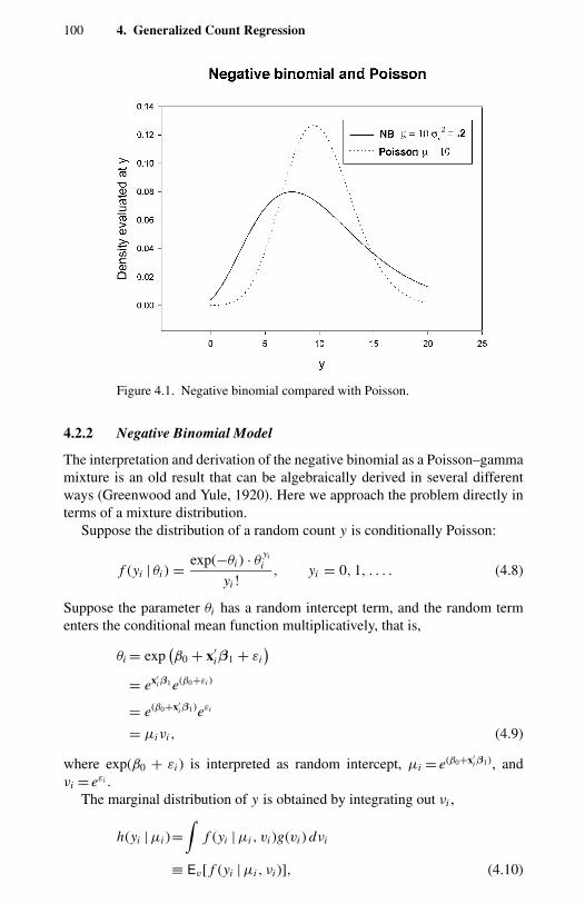
100 4. Generalized Count Regression

Figure 4.1. Negative binomial compared with Poisson.

4.2.2 Negative Binomial Model

The interpretation and derivation of the negative binomial as a Poisson–gammamixture is an old result that can be algebraically derived in several differentways (Greenwood and Yule, 1920). Here we approach the problem directly interms of a mixture distribution.

Suppose the distribution of a random count y is conditionally Poisson:

f (yi | θi ) = exp(−θi ) · θyi

i

yi !, yi = 0, 1, . . . . (4.8)

Suppose the parameter θi has a random intercept term, and the random termenters the conditional mean function multiplicatively, that is,

θi = exp(β0 + x′

iβ1 + εi)

= ex′iβ1 e(β0+εi )

= e(β0+x′iβ1)eεi

= µiνi , (4.9)

where exp(β0 + εi ) is interpreted as random intercept, µi = e(β0+x′iβ1), and

νi = eεi .The marginal distribution of y is obtained by integrating out νi ,

h(yi | µi )=∫

f (yi | µi , vi )g(vi ) dνi

≡ Ev[ f (yi | µi , νi )], (4.10)

4.2. Mixture Models for Unobserved Heterogeneity 101

where g(νi ) is a mixing distribution. For specific choices of f (·) and g(·), forexample Poisson and gamma densities respectively, the integral has an explicitsolution. This is shown shortly.

From here on the i subscript is omitted if there is no ambiguity. Suppose thatthe variable ν has a two-parameter gamma distribution g(ν; δ, φ)

g(ν, δ, φ) = δφ

(δ)νδ−1e−νφ, δ > 0, φ > 0, (4.11)

where E[ν] = δ/φ, and V[ν] = δ/φ2. The intercept identification condition isE[ν] = 1 which is obtained by setting δ = φ, which implies a one-parametergamma family with V[ν] = 1/δ ≡ α. We transform from ν to θ using θ = µν,and noting that the Jacobian transformation term is (1/µ). This yields the pdffor θ ,

g(θ | µ, δ)= 1

µ

δδ

(δ)

(θ

µ

)δ−1

e− θµδ

= (δ/µ)δ

(δ)θδ−1e− θδ

µ . (4.12)

The marginal distribution of y is given by

h(y | µ, δ) =∫

exp(−θ ) · θ y

y!

(δ/µ)δ

(δ)θδ−1e− θδ

µ dθ. (4.13)

Using the following definitions this integral can be expressed in a closed form:

(a) =∫ ∞

0ta−1e−t dt, for any a > 0

(y − 1) = y!

(a)/ba =∫ ∞

0ta−1e−bt dt, for any b > 0.

Substituting these into (4.13) we obtain

h(y | µ, δ)= (δ/µ)δ

(δ)(y + 1)

∫exp

(−θ

(1 + δ

µ

))θ y+δ−1dθ

=(

δµ

)δ(1 + δ

µ

)−(δ+y)(δ + y)

(δ)(y + 1)

= (α−1 + y)

(α−1)(y + 1)

(α−1

α−1 + µ

)α−1(µ

µ + α−1

)y

,

(4.14)

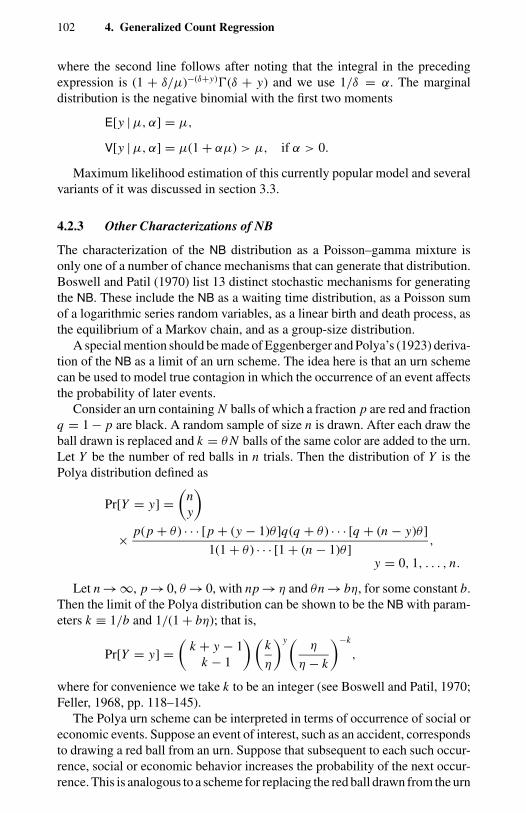
102 4. Generalized Count Regression

where the second line follows after noting that the integral in the precedingexpression is (1 + δ/µ)−(δ+y)(δ + y) and we use 1/δ = α. The marginaldistribution is the negative binomial with the first two moments

E[y | µ, α] = µ,

V[y | µ, α] = µ(1 + αµ) > µ, if α > 0.

Maximum likelihood estimation of this currently popular model and severalvariants of it was discussed in section 3.3.

4.2.3 Other Characterizations of NB

The characterization of the NB distribution as a Poisson–gamma mixture isonly one of a number of chance mechanisms that can generate that distribution.Boswell and Patil (1970) list 13 distinct stochastic mechanisms for generatingthe NB. These include the NB as a waiting time distribution, as a Poisson sumof a logarithmic series random variables, as a linear birth and death process, asthe equilibrium of a Markov chain, and as a group-size distribution.

A special mention should be made of Eggenberger and Polya’s (1923) deriva-tion of the NB as a limit of an urn scheme. The idea here is that an urn schemecan be used to model true contagion in which the occurrence of an event affectsthe probability of later events.

Consider an urn containing N balls of which a fraction p are red and fractionq = 1 − p are black. A random sample of size n is drawn. After each draw theball drawn is replaced and k = θ N balls of the same color are added to the urn.Let Y be the number of red balls in n trials. Then the distribution of Y is thePolya distribution defined as

Pr[Y = y] =(

ny

)× p(p + θ ) · · · [p + (y − 1)θ ]q(q + θ ) · · · [q + (n − y)θ ]

1(1 + θ ) · · · [1 + (n − 1)θ ],

y = 0, 1, . . . , n.

Let n → ∞, p → 0, θ → 0, with np → η and θn → bη, for some constant b.Then the limit of the Polya distribution can be shown to be the NB with param-eters k ≡ 1/b and 1/(1 + bη); that is,

Pr[Y = y] =(

k + y − 1k − 1

)(k

η

)y(η

η − k

)−k

,

where for convenience we take k to be an integer (see Boswell and Patil, 1970;Feller, 1968, pp. 118–145).

The Polya urn scheme can be interpreted in terms of occurrence of social oreconomic events. Suppose an event of interest, such as an accident, correspondsto drawing a red ball from an urn. Suppose that subsequent to each such occur-rence, social or economic behavior increases the probability of the next occur-rence. This is analogous to a scheme for replacing the red ball drawn from the urn

4.2. Mixture Models for Unobserved Heterogeneity 103

in such a way that the proportion of red balls to black balls increases. If, however,after a ball is drawn, more balls of opposite color are added to the urn, then thedrawing of a ball reduces the probability of a repeat occurrence at the next draw.

Of course, there can be many possible replacement schemes in the urn prob-lem. Which scheme one uses determines the nature of the dependence betweenone event and the subsequent ones. This shows that the NB distribution canreflect true contagion or occurrence dependence. By contrast, an example ofspurious contagion results if we consider that different individuals, for exam-ple, workers, experience an event, such as an accident at the workplace, withconstant but different probabilities. This is analogous to individuals havingtheir separate urns with red and black balls in different proportions. For eachperson the probability of drawing a red ball is constant, but there is a distribu-tion across individuals. In the aggregate one observes apparent dependence, orspurious contagion, due to heterogeneity.

4.2.4 General Mixture Results

The statistics literature contains many examples of generalized count modelsgenerated by mixtures. An historical account can be found in Johnson, Kotz,and Kemp (1992). Although the negative binomial is one of the oldest and mostpopular in applied work, other mixtures that have been used include Poisson-inverse Gaussian mixture (Dean, Lawless, and Willmot, 1989), discrete log-normal (Shaban, 1988), generalized Poisson (Consul, 1989; Consul and Jain,1973), and Gauss-Poisson (Johnson, Kotz, and Kemp, 1992). Additional flex-ibility due to the presence of parameters of the mixing distribution generallyimproves the fit of the resulting distribution to observed data.

Many general probability distributions can collapse to special forms underrestrictions on a subset of parameters. These then provide natural generaliza-tions of the restrictive cases. One of the oldest approaches to the generalizationof the Poisson is based on mixtures and convolutions. Of course, the samedistribution could be postulated directly as a more flexible functional form.Furthermore, a particular mixture could arise from component distributions inmore than one way; that is, it may not be a unique convolution.

It is useful to distinguish between continuous mixtures (convolutions) andfinite mixtures.

Definition. Suppose F(y | θ ) is a parametric distribution depending on θ , andlet π (θ | α) define a continuous mixing distribution. Then a convolution or acontinuous mixture is defined by F(y | α) = ∫∞

−∞ π (θ | α)F(y | θ ) dθ .

Definition. If Fj (y | θ j ), j = 1, 2, . . . , m, is a distribution function then F(y | π j )=∑m

j = 1 π j Fj (y | θ j ), 0 < π j < 1,∑m

j = 1 π j = 1, defines m-component finitemixture.

Note that although these definitions are stated in terms of the cdf rather thanthe pdf, definitions in terms of the latter are feasible. The second definition is a

104 4. Generalized Count Regression

special case of the first, if π (θ | α) is discrete and assigns positive probabilityto a finite number of parameter values θ1, . . . , θm . In this case π j , the mixingproportion, is the probability that an observation comes from the j th population.By contrast, in a continuous mixture the parameter θ of the conditional densityis subject to chance variation described by a density with an infinite number ofsupport points. Estimation and inference for convolutions involves (θ, α) andfor finite mixtures (π j , θ j ; j = 1, . . . , m).

4.2.5 Identification

The identifiability, or unique characterization, of mixtures should be establishedprior to estimation and inference. A mixture is identifiable if there is a uniquecorrespondence between the mixture and the mixing distribution, usually in thepresence of some a priori constraints (Teicher, 1961).

The pgf of a mixed Poisson model, denoted P(z), can be expressed as theconvolution integral

P(z) =∫ ∞

0exp(µ(z − 1)) f (µ) dµ, (4.15)

where exp(µ(z−1)) is the pgf of the Poisson distribution and f (µ) is the assumeddistribution for µ. The mixture models, being akin to “reduced form” models,are subject to an identification problem. The same distribution can be obtainedfrom a different mixture. For example, the negative binomial mixture can begenerated as a Poisson–gamma mixture by allowing the Poisson parameter µ tohave a gamma distribution (see section 4.2). It can also be generated by taking arandom sum of independent random variables in which the number of terms inthe sum has a Poisson distribution; if each term is discrete and has a logarithmicdistribution and if the number of terms has a Poisson distribution, the mixtureis negative binomial (Daley and Vere-Jones, 1988).

Identification may be secured by restricting the conditional event distribu-tion to be Poisson. This follows from the uniqueness property of exponentialmixtures (Jewel, 1982).

A practical consideration is that in applied work, especially that based onsmall samples, it may be difficult to distinguish between alternative mixingdistributions, and the choice may be largely based on the ease of computation.Most of the issues are analogous to those that have been discussed extensivelyin the duration literature.∗ In the examples in the duration literature finiteness ofthe mean of the mixing distribution is required for identifiability of the mixture.This issue is illustrated by comparing the Poisson–gamma and Poisson–inverseGaussian (PIG) mixtures. The latter is generated from the convolution integral∫

f (yi | µi , νi )g(νi ) dνi with f (·) as Poisson and g(·) as inverse Gaussian with

∗ Lancaster (1990, chapter 7) provides an excellent discussion of the identification conditions forthe proportional hazard models and gives an example of a nonidentifiable model.

4.2. Mixture Models for Unobserved Heterogeneity 105

density

g(v) = (2πδ−1ν3) exp

[−δ(ν − 1)2

2ν

], (4.16)

where E[ν] = 1, V[ν] = δ−1 ≡ α. Although the convolution integral doesnot have a closed form, note that the first two moments of the mixing inverseGaussian distribution are the same as those of the gamma distribution in (4.11).Consequently, the first two moments of the Poisson–gamma and PIG mixturesare equal. Hence, the two mixing distributions can only be distinguished usinginformation about higher moments. In small samples such information is im-precise, and attempts to distinguish empirically between competing alternativesmay yield inconclusive results.

Although more flexible count distributions are usually derived by mixing, itmay sometimes be appropriate to directly specify flexible functional forms forcounts, without the intermediate step of introducing a distribution of unobservedheterogeneity (e.g., in aggregate time series applications). In microeconometricapplications, however, mixing seems a natural way of handling heterogeneity.

As an example, Dean, Lawless, and Wilmot (1989) use the PIG mixture tostudy the frequency of insurance claims. They analyze data on the number ofaccident claims on third-party motor insurance policies in Sweden during 1977in each of 315 risk groups. The counts take a wide range of values – the medianis 10, the maximum is 2127 – so there is clearly a need to control for the sizeof risk group. This is done by defining the mean to equal Ti exp(xiβ), whereTi is the number of insured automobile-years for the group, which is equiva-lent to including ln Ti as a regressor and constraining its coefficient to equalunity. Even after including this and other regressors, the data are overdispersed.The authors estimate a mixed PIG model, with overdispersion modeled by aquadratic variance function. These maximum likelihood estimates are within1% of estimates from solving equations that use only the first two moments.

4.2.6 Consequences of Misspecified Heterogeneity

In the duration literature, in which the shape of the hazard function is of centralinterest, there has been an extensive discussion of how misspecified unobservedheterogeneity can lead to inconsistent estimates of the hazard function (seeHeckman and Singer, 1984, and Lancaster, 1990, pp. 294–305 for a summary).Under our assumptions, misspecification of the heterogeneity distribution im-plies that the variance function, and the marginal distribution of counts, are mis-specified. The consequences of this misspecification are dealt with in Chapter 2.A particular parametric assumption of heterogeneity is not easy to justify exceptas an approximation. Obviously, the more flexible is the assumption, the lesslikely is a serious misspecification error. Certain variance functions have beenfound to be good approximations to arbitrary variance functions in the sensethat the improvement in fit of the model achieved by freeing up the form of the

106 4. Generalized Count Regression

variance function further may be slight. An example is NB2 quadratic variancefunction. Also see Bourlange and Doz (1988).

4.3 Models Based on Waiting-Time Distributions

Chapter 1 sketches the duality between waiting-time distributions and eventcount distributions in a simple case. We pursue this issue in greater detail here.Some useful insights into the dispersion properties of counts are obtained byexamining the duality between waiting times and event counts in a model inwhich the waiting times are dependent.

4.3.1 True and Apparent Contagion

The discussion of heterogeneity and overdispersion is related to a long-standingdiscussion in the biostatistics literature on true and apparent contagion. Truecontagion refers to dependence between the occurrence of successive events.The occurrence of an event, such as an accident or illness, may change theprobability of subsequent occurrence of similar events. True positive contagionimplies that the occurrence of an event shortens the expected waiting time tothe next occurrence of the event, whereas true negative contagion implies thatthe expected waiting time to the next occurrence of the event is longer. Thealleged phenomenon of accident proneness can be interpreted in terms of truecontagion as suggesting that an individual who has experienced an accidentis more likely to experience another accident. Apparent contagion arises fromthe recognition that sampled individuals come from a heterogeneous popula-tion in which individuals have constant but different propensity to experienceaccidents. For a given individual, occurrence of an accident does not make itmore or less likely that another accident will occur. But aggregation acrossheterogeneous individuals generates the statistical finding that occurrence ofan accident increases the probability of another accident.

Yet another mode of dynamic dependence is present in the notion that eventsoccur in “spells” that themselves occur independently according to some prob-ability law. Events within a given spell follow a different probability law andmay be dependent. Serial dependence can be shown to lead to overdispersionin the counts. However, as was shown previously, overdispersion can also be aconsequence of population heterogeneity or differences among individuals intheir propensity to experience an event. Thus, the mere presence of overdis-persion in the data does not preclude the possibility that for a given individualthere may be no serial dependence in event occurrence. This second situationis therefore referred to as apparent contagion.

The discussion of accident proneness of individuals in the early statisti-cal literature emphasized the difficulty of distinguishing between true accidentproneness and effects of interindividual heterogeneity. In reference to Neyman(1939), Feller (1943) pointed out that the same negative binomial model had

4.3. Models Based on Waiting-Time Distributions 107

been derived by Greenwood and Yule (1920) using the assumption of popula-tion heterogeneity and by Eggenberger and Polya (1923), who assumed truecontagion. He observed, “Therefore, the possibility of its interpretation in twoways, diametrically opposite in their nature as well as their implications is ofgreatest statistical significance” (Feller, 1943, p. 389). Neyman (1965, p. 6)emphasized that the distinction between true and apparent contagion would be-come possible “if one has at one’s disposal data on accidents incurred by eachindividual separately for two periods of six months each”; clearly this refers tolongitudinal data. These issues are further pursued in Chapter 9.

4.3.2 Renewal Process

Renewal theory deals with functions of iid nonnegative random variables thatrepresent time intervals between successive events (renewals). The topic isintroduced in Chapter 1.

Consider the counting process, N (t), t ≥ 0, which measures the successiveoccurences of an event in the time interval (0, t]. Denote by Wr the length oftime between the occurrences of events (r − 1) and r , by Fn(t) the cdf of(W1, . . . , Wn), and by Sn the sum of waiting times,

∑nk = 1 Wk , for n events,

n ≥ 1. Renewal theory derives properties of random variables associated withthe number or events, N (t), or waiting times, Sn , given the specification of Fn(t).An example of a statistic of major interest is the mean number of occurrencesin the interval (0, t], denoted as m(t) and called the renewal function, which isrelated to Fn(t). This is evaluated at t = T,

m(t)=E[N (T )]

=∞∑

n = 1

n Pr[N (T ) = n]

=∞∑

n = 1

n[Fn(T ) − Fn + 1(T )]

=∞∑

n = 1

Fn(T ). (4.17)

Thus, the mean of the count variable is∑∞

n = 1 Fn(T ) and its variance is given by

V[N ] =∞∑

n = 1

n2[Fn(T ) − Fn + 1(T )] −( ∞∑

n = 1

Fn(T )

)2

. (4.18)

4.3.3 Waiting-Time Distribution

Here we consider the mathematical relation between counts and waiting timesthat was introduced in Chapter 1. Although a general formulation is possible,

108 4. Generalized Count Regression

it does not produce easily interpretable results. Instead we present a specificexample, due to Winkelmann (1995), that illustrates both the issues and themethod.

For events that occur randomly over time, the count point process is N(t),t > 0. Let N (t) represent the number of events between 0 and T . For fixed t ,N (t) is a count variable. This can be transformed into the sequence of intereventwaiting times, denoted Wr for the time interval between the (r − 1)th and r th

events. The arrival time of the r th event is given by Sr =∑rj = 1 W j . For a re-

newal process, the distribution of Sr can be derived by using Laplace transforms.Given the definitions, NT < r iff Sr > T . Let Fr (T ) denote the cumulative

distribution of Sr . Then

Pr[N (T ) < r ] = Pr[Sr ≥ T ]

= 1 − Fr (T ) (4.19)

and

Pr[N (T ) = r ] = Pr[N (T ) < r + 1] − Pr[N (T ) < r ]

= Fr (T ) − Fr+1(T )

=∫ T

0[1 − Fr (T − z)] dFr (z), (4.20)

which is the fundamental relation between the distribution of waiting timesand that of event counts. This relation may form the basis of a count modelcorresponding to an arbitrary waiting-time model. Conditioning on exogenousvariable xi , the likelihood for the m independent observations is defined by

L =m∏

i = 1

[Fni (T | xi ) − Fni +1(T | xi )

]. (4.21)

The practical utility of this formulation in part depends on whether the cdf ofSn can be easily evaluated. Even if no closed form expression for the cdf isavailable, computer-intensive methods can be used as suggested by Lee (1997).Further, the approach can be extended to generalized renewal processes; forexample, we may allow the waiting-time distribution of the first event to differfrom that of subsequent events (Ross, 1996) – a case analogous to the hurdlecount model. Another potential advantage is that the approach can exploit theavailability of structurally and behaviorally richer specifications of waiting-timemodels.

One approach is to begin by specifying parametric regression models forwaiting times. For example, a broad class of parametric waiting-time models isdefined by the regression

ln ti = x′iβ + σεi (4.22)

where the distribution of εi is specified. We consider some special cases.

4.3. Models Based on Waiting-Time Distributions 109

• The exponential duration model (and the Poisson model for counts)follows from the assumption that σ = 1, and εi follow the extremevalue distribution.

• A less restrictive model is

ln ti = x′iβ + εi − ui

where the εi are iid extreme value distributed and ui is a log-gammarandom variable.∗ This choice corresponds to the negative binomialdistribution for counts (Lee, 1997).

• Equation (4.22) corresponds to the popular Weibull waiting-time dis-tribution with an additional free parameter that allows duration depen-dence. In this case there is no closed form expression for the distribu-tion of counts.

In the following subsection we consider an interesting special case analyzedby Winkelmann (1995), which illustrates some of the problems and possibilitiesof this approach.

4.3.4 Gamma Waiting Times

Winkelmann (1995) considered the gamma waiting-time distribution, whichadmits monotonic increasing or decreasing hazards. Then the density of W isgiven by

f (W | φ, α) = αφ

(φ)W α−1e−αW , W > 0. (4.23)

The corresponding hazard function, which describes the underlying dependenceof the process, is defined as

h(W )= f (W )

1 − F(W )

=− d

dWln(1 − F(W ))

=[ ∫ ∞

0e−αu(1 + u/W )φ−1 du

]−1

.

The hazard function does not have a closed-form expression but can beshown to be monotonically increasing for α > 1. This implies positive durationdependence or increasing hazards. The function is monotonic decreasing forα < 1, which implies negative duration dependence or decreasing hazards.The slope of the hazard function, ∂h(W )/∂W , reflects the dependence of the

∗ The density of u is defined by f (v) = exp[v/η−exp(v)]/(1/η) where u = ln η+v (Kalbfleishand Prentice, 1980; Lee, 1997).

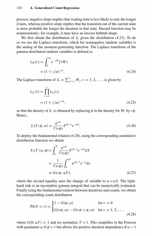
110 4. Generalized Count Regression

process; negative slope implies that waiting time is less likely to end, the longerit lasts, whereas positive slope implies that the transition out of the current stateis more probable the longer the duration in that state. Hazard function may benonmonotonic; for example, it may have an inverse bathtub shape.

We first obtain the distribution of Sr given the distribution (4.23). To doso we use the Laplace transform, which for nonnegative random variables isthe analog of the moment-generating function. The Laplace transform of thegamma-distributed random variables is defined as

LW (z) =∫ ∞

0e−zW f (W )

= (1 + z/α)−α. (4.24)

The Laplace transform of Sr =∑rj = 1 W j , r = 1, 2, . . . , is given by

LSr (z) =r∏

i = 1

LSi (z)

= (1 + z/α)−rα, (4.25)

so that the density of Sr is obtained by replacing φ in the density for Wi by rφ.Hence,

fr (S | φ, α) = αrφ

(rφ)Srφ−1e−αS. (4.26)

To deploy the fundamental relation (4.20), using the corresponding cumulativedistribution function we obtain

Fr (T | α, φ)=∫ T

0

αrφ

(rφ)Srφ−1e−αSd S

= 1

(rφ)

∫ αT

0urφ−1e−udu

≡ G(rφ, αT ), (4.27)

where the second equality uses the change of variable to u = αS. The right-hand side is an incomplete gamma integral that can be numerically evaluated.Finally using the fundamental relation between durations and counts, we obtainthe corresponding count distribution

Pr[N = r ] =

1 − G(φ, α) for r = 0

G(rφ, α) − G(rφ + φ, α) for r = 1, 2, . . . .

(4.28)

where G(0, αT ) = 1 and we normalize T = 1. This simplifies to the Poissonwith parameter α if φ = 1 but allows for positive duration dependence if α > 1

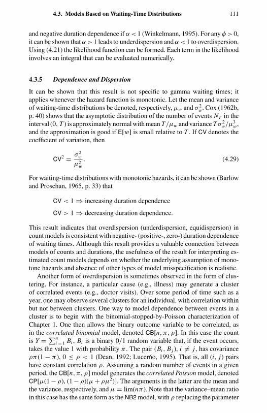
4.3. Models Based on Waiting-Time Distributions 111

and negative duration dependence if α < 1 (Winkelmann, 1995). For any φ > 0,it can be shown that α > 1 leads to underdispersion and α < 1 to overdispersion.Using (4.21) the likelihood function can be formed. Each term in the likelihoodinvolves an integral that can be evaluated numerically.

4.3.5 Dependence and Dispersion

It can be shown that this result is not specific to gamma waiting times; itapplies whenever the hazard function is monotonic. Let the mean and varianceof waiting-time distributions be denoted, respectively, µw and σ 2

w. Cox (1962b,p. 40) shows that the asymptotic distribution of the number of events NT in theinterval (0, T ) is approximately normal with mean T/µw and variance T σ 2

w/µ3w,

and the approximation is good if E[w] is small relative to T . If CV denotes thecoefficient of variation, then

CV2 = σ 2w

µ2w

. (4.29)

For waiting-time distributions with monotonic hazards, it can be shown (Barlowand Proschan, 1965, p. 33) that

CV < 1 ⇒ increasing duration dependence

CV > 1 ⇒ decreasing duration dependence.

This result indicates that overdispersion (underdispersion, equidispersion) incount models is consistent with negative- (positive-, zero-) duration dependenceof waiting times. Although this result provides a valuable connection betweenmodels of counts and durations, the usefulness of the result for interpreting es-timated count models depends on whether the underlying assumption of mono-tone hazards and absence of other types of model misspecification is realistic.

Another form of overdispersion is sometimes observed in the form of clus-tering. For instance, a particular cause (e.g., illness) may generate a clusterof correlated events (e.g., doctor visits). Over some period of time such as ayear, one may observe several clusters for an individual, with correlation withinbut not between clusters. One way to model dependence between events in acluster is to begin with the binomial-stopped-by-Poisson characterization ofChapter 1. One then allows the binary outcome variable to be correlated, asin the correlated binomial model, denoted CB[n, π, ρ]. In this case the countis Y = ∑n

i = 1 Bi , Bi is a binary 0/1 random variable that, if the event occurs,takes the value 1 with probability π . The pair (Bi , B j ), i = j , has covarianceρπ (1 − π ), 0 ≤ ρ < 1 (Dean, 1992; Lucerno, 1995). That is, all (i, j) pairshave constant correlation ρ. Assuming a random number of events in a givenperiod, the CB[n, π, ρ] model generates the correlated Poisson model, denotedCP[µ(1 − ρ), (1 − ρ)(µ + ρµ2)]. The arguments in the latter are the mean andthe variance, respectively, and µ = lim(nπ ). Note that the variance–mean ratioin this case has the same form as the NB2 model, with ρ replacing the parameter

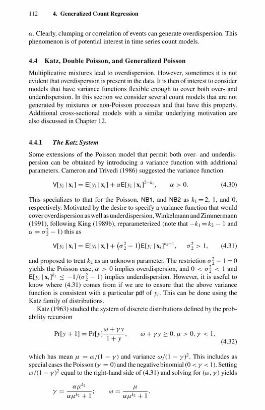
112 4. Generalized Count Regression

α. Clearly, clumping or correlation of events can generate overdispersion. Thisphenomenon is of potential interest in time series count models.

4.4 Katz, Double Poisson, and Generalized Poisson

Multiplicative mixtures lead to overdispersion. However, sometimes it is notevident that overdispersion is present in the data. It is then of interest to considermodels that have variance functions flexible enough to cover both over- andunderdispersion. In this section we consider several count models that are notgenerated by mixtures or non-Poisson processes and that have this property.Additional cross-sectional models with a similar underlying motivation arealso discussed in Chapter 12.

4.4.1 The Katz System

Some extensions of the Poisson model that permit both over- and underdis-persion can be obtained by introducing a variance function with additionalparameters. Cameron and Trivedi (1986) suggested the variance function

V[yi | xi ] = E[yi | xi ] + αE[yi | xi ]2−k1 , α > 0. (4.30)

This specializes to that for the Poisson, NB1, and NB2 as k1 = 2, 1, and 0,respectively. Motivated by the desire to specify a variance function that wouldcover overdispersion as well as underdispersion, Winkelmann and Zimmermann(1991), following King (1989b), reparameterized (note that −k1 = k2 − 1 andα = σ 2

2 − 1) this as

V[yi | xi ] = E[yi | xi ] + (σ 22 − 1

)E[yi | xi ]

k2+1, σ 22 > 1, (4.31)

and proposed to treat k2 as an unknown parameter. The restriction σ 22 − 1 = 0

yields the Poisson case, α > 0 implies overdispersion, and 0 < σ 22 < 1 and

E[yi | xi ]k2 ≤ −1/(σ 22 − 1) implies underdispersion. However, it is useful to

know where (4.31) comes from if we are to ensure that the above variancefunction is consistent with a particular pdf of yi . This can be done using theKatz family of distributions.

Katz (1963) studied the system of discrete distributions defined by the prob-ability recursion

Pr[y + 1] = Pr[y]ω + γ y

1 + y, ω + γ y ≥ 0, µ > 0, γ < 1,

(4.32)

which has mean µ = ω/(1 − γ ) and variance ω/(1 − γ )2. This includes asspecial cases the Poisson (γ = 0) and the negative binomial (0 < γ < 1). Settingω/(1 − γ )2 equal to the right-hand side of (4.31) and solving for (ω, γ ) yields

γ = αµk2

αµk2 + 1; ω = µ

αµk2 + 1.

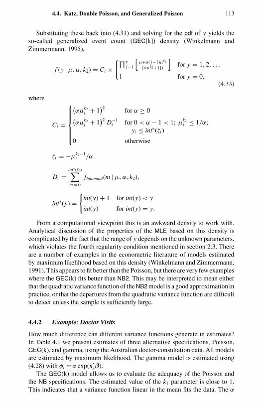
4.4. Katz, Double Poisson, and Generalized Poisson 113

Substituting these back into (4.31) and solving for the pdf of y yields theso-called generalized event count (GEC[k]) density (Winkelmann andZimmermann, 1995),

f (y | µ, α, k2) = Ci ×∏y

j=1

[µ+α( j−1)µk2

[αµk2 +1] j

]for y = 1, 2, . . .

1 for y = 0,

(4.33)

where

Ci =

(αµ

k2i + 1

)ζi for α ≥ 0(αµ

k2i + 1

)ζi D−1i for 0 < α − 1 < 1; µ

k2i ≤ 1/α;

yi ≤ int∗(ζi )

0 otherwise

ζi = −µk2−1i /α

Di =int∗(ζi )∑m = 0

fbinomial(m | µ, α, k2),

int∗(y) =

int(y) + 1 for int(y) < y

int(y) for int(y) = y.

From a computational viewpoint this is an awkward density to work with.Analytical discussion of the properties of the MLE based on this density iscomplicated by the fact that the range of y depends on the unknown parameters,which violates the fourth regularity condition mentioned in section 2.3. Thereare a number of examples in the econometric literature of models estimatedby maximum likelihood based on this density (Winkelmann and Zimmermann,1991). This appears to fit better than the Poisson, but there are very few exampleswhere the GEC(k) fits better than NB2. This may be interpreted to mean eitherthat the quadratic variance function of the NB2 model is a good approximation inpractice, or that the departures from the quadratic variance function are difficultto detect unless the sample is sufficiently large.

4.4.2 Example: Doctor Visits

How much difference can different variance functions generate in estimates?In Table 4.1 we present estimates of three alternative specifications, Poisson,GEC(k), and gamma, using the Australian doctor-consultation data. All modelsare estimated by maximum likelihood. The gamma model is estimated using(4.28) with φi = α exp(x′

iβ).The GEC(k) model allows us to evaluate the adequacy of the Poisson and

the NB specifications. The estimated value of the k1 parameter is close to 1.This indicates that a variance function linear in the mean fits the data. The α

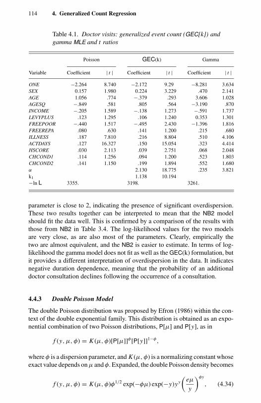
114 4. Generalized Count Regression

Table 4.1. Doctor visits: generalized event count (GEC[k]) andgamma MLE and t ratios

Poisson GEC(k) Gamma

Variable Coefficient | t | Coefficient | t | Coefficient | t |

ONE −2.264 8.740 −2.172 9.29 −8.281 3.634SEX 0.157 1.980 0.224 3.229 .470 2.141AGE 1.056 .774 −.379 .293 3.606 1.028AGESQ −.849 .581 .805 .564 −3.190 .870INCOME −.205 1.589 −.138 1.273 −.591 1.737LEVYPLUS .123 1.295 .106 1.240 0.353 1.301FREEPOOR −.440 1.517 −.495 2.430 −1.396 1.816FREEREPA .080 .630 .141 1.200 .215 .680ILLNESS .187 7.810 .216 8.804 .510 4.106ACTDAYS .127 16.327 .150 15.054 .323 4.414HSCORE .030 2.113 .039 2.751 .068 2.048CHCOND1 .114 1.256 .094 1.200 .523 1.803CHCOND2 .141 1.150 .199 1.894 .552 1.680α 2.130 18.775k1 1.138 10.194

.235 3.821

−ln L 3355. 3198. 3261.

parameter is close to 2, indicating the presence of significant overdispersion.These two results together can be interpreted to mean that the NB2 modelshould fit the data well. This is confirmed by a comparison of the results withthose from NB2 in Table 3.4. The log-likelihood values for the two modelsare very close, as are also most of the parameters. Clearly, empirically thetwo are almost equivalent, and the NB2 is easier to estimate. In terms of log-likelihood the gamma model does not fit as well as the GEC(k) formulation, butit provides a different interpretation of overdispersion in the data. It indicatesnegative duration dependence, meaning that the probability of an additionaldoctor consultation declines following the occurrence of a consultation.

4.4.3 Double Poisson Model

The double Poisson distribution was proposed by Efron (1986) within the con-text of the double exponential family. This distribution is obtained as an expo-nential combination of two Poisson distributions, P[µ] and P[y], as in

f (y, µ, φ) = K (µ, φ)[P[µ]]φ[P[y]]1−φ,

where φ is a dispersion parameter, and K (µ, φ) is a normalizing constant whoseexact value depends on µ and φ. Expanded, the double Poisson density becomes

f (y, µ, φ) = K (µ, φ)φ1/2 exp(−φµ) exp(−y)yy

(eµ

y

)φy

, (4.34)

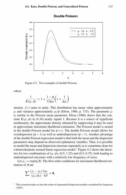
4.4. Katz, Double Poisson, and Generalized Poisson 115

Figure 4.2. Two examples of double Poisson.

where

1

K (µ, φ) 1 + 1 − φ

12φµ

(1 + 1

φµ

)ensures f (·) sums to unity. This distribution has mean value approximatelyµ and variance approximately µ/φ (Efron, 1986, p. 715). The parameter µ

is similar to the Poisson mean parameter. Efron (1986) shows that the con-stant K (µ, φ) in (4.34) nearly equals 1. Because it is a source of significantnonlinearity, the approximate density obtained by suppressing it may be usedin approximate maximum likelihood estimation. The Poisson model is nestedin the double Poisson model for φ = 1. The double Poisson model allows foroverdispersion (φ < 1) as well as underdispersion (φ > 1). Another advantageof the double Poisson regression model is that both the mean and the dispersionparameters may depend on observed explanatory variables. Thus, it is possibleto model the mean and dispersion structure separately as is sometimes done fora heteroskedastic normal linear regression model.∗ Figure 4.2 shows the densi-ties for two combinations of (µ, φ), (0.5, 1.25) and (0.5, 0.75), both leading tounderdispersed outcomes with a relatively low frequency of zeros.

Let µi = exp(x′iβ). The first-order conditions for maximum likelihood esti-

mation of β are∑ (yi − µi )

(µi/φi )

∂µi

∂β= 0,

∗ This extension takes us into the realm of exponential dispersion models considered by Jorgensen(1987).

116 4. Generalized Count Regression

which are the same as for the PML if φi is a constant and does not involvecovariates. If φ is a constant, the maximum likelihood estimate φ is simply theaverage value of the deviance measure,

φ = n−1∑

yi ln yi/µi − (yi − µi ). (4.35)

Because the estimating equations forβ are the same as in the Poisson case, PMLis consistent even if the dgp is double Poisson. A simple way of adjusting itsvariance is to scale the estimated variance matrix by multiplying by 1/φ. How-ever, to calculate the event probabilites, the expression in (4.34) should be used.

4.4.4 Neyman’s Contagious Distributions

Neyman (1939) developed type A, type B, and type C distributions to handlea form of clustering that is common in the biological sciences. The univariateversion of type A has been used with success, but we are unaware of anyregression applications. Johnson, Kotz, and Kemp (1992) give an excellentaccount of its properties and further references.

These distributions can be thought of as compound Poisson distributionsthat involve two processes. For example, suppose that the number of events(e.g., doctor visits) within a spell (of illness), denoted y, follows the Pois-son distribution, and the random number of spells within a specified period,denoted z, follows some other discrete distribution. Then the marginal distri-bution of events is compound Poisson. One variant of Neyman type A withtwo parameters is obtained if both y and z have independent Poisson distribu-tions parameters (say) µ and λ, respectively. The expression for the compounddistribution can be obtained by specializing the general result in (4.15).

In univariate cases Neyman type A and negative binomial have been com-pared. They are close competitors. Because the latter is better established inregression contexts, we shall not devote further space to Neyman type A.

4.4.5 Consul’s Generalized Poisson

Consul (1989) has proposed a distribution that can accommodate both over-and underdispersion. The distribution is

f (yi | xi ) =

exp(−µi −γ yi )(µi +γ yi )yi −1

yi !, yi = 0, 1, . . . ,

0 for y > N , when γ < 0,

(4.36)

where max(−1, −µ/N ) < γ ≤ 1 and N is the largest positive integer thatsatisfies the inequality µ + Nγ > 0 if µ is large. Because E[yi ] = µ(1 − γ )−1

and V[yi ] = µ(1−γ )−3, the distribution can display under- and equidispersionas max(−1, −µ/N ) < γ ≤ 0, and γ = 0, and overdispersion for 0 < γ < 1.

4.5. Truncated Counts 117

This model does not appear to have been much used in regression contexts(see Consul and Famoye, 1992). Because for this distribution the range ofthe random variable depends on the unknown parameter γ , one of the standardconditions for consistency and asymptotic normality of the maximum likelihoodestimation is violated. The importance of this violation is a matter for futureinvestigation.

4.5 Truncated Counts

The models allowing for truncation are required if observations (yi , xi ) in somerange are totally lost and the distribution of observed counts is restricted. Insome studies involving count data, inclusion in the sample requires that sampledindividuals have been engaged in the activity of interest or, as Johnson and Kotz(1969, p. 104) put it, “the observational apparatus become active only when aspecified number of events (usually one) occurs.” Examples of truncated countsinclude the number of bus trips made per week in surveys taken on buses, thenumber of shopping trips made by individuals sampled at a mall, and the numberof unemployment spells among a pool of unemployed. These are examples ofleft truncation or truncation from below. Right truncation, or truncation fromabove, may result if high counts are not observed. In the special case of a“positive Poisson” model zeros are not observed.

Truncated count models are discrete counterparts of truncated and censoredmodels for continuous variables, particularly the Tobit models for normallydistributed data, that have been used extensively in the economics literature(Amemiya, 1984; Maddala, 1983). The sample selection counterparts of themodel are discussed in Chapter 11. Truncated models are also related to the hur-dle model discussed in section 4.7.

4.5.1 Standard Truncated Models

For simplicity, only truncation from below is considered. Analogous resultsfor right truncation can be derived by adapting those for left truncation. Thefollowing general framework for truncated count models is used. Let

H (yi ,Λ) = Pr[Yi ≤ yi ]

denote the cdf of the discrete random variable with pdf h(yi ,Λ), where Λ is aparameter vector. If realizations of y less than a positive integer r are omitted,the ensuing distribution is called left-truncated (or truncated from below). Theleft-truncated count distribution is given by

f (yi ,Λ | yi ≥ r ) = h(yi ,Λ)

1 − H (r − 1,Λ), yi = r, r + 1, . . . .

(4.37)

118 4. Generalized Count Regression

A special case is the left-truncated negative binomial for which

h(yi ,Λ) = (yi + α−1)

(α−1)(yi + 1)(αµi )

yi (1 + αµi )−(yi +α−1),

where Λ ≡ (µi , α). The truncated mean and variance are defined by

θi = µi + δi

σ 2i = µi + αµ2

i − δi (µi − r )

δi = µi [1 + α(r − 1)]λ(r − 1, µi , α)

λ(r − 1, µi , α) = h(r − 1, µi )/1 − H (r − 1, µi ).

(4.38)

The left-truncated NB incorporates overdispersion in the sense that truncatedvariance of the NB exceeds the truncated variance of the Poisson. The latter isa limiting case obtained as α → 0.

For the Poisson pdf h(yi , µi ) = exp(−µi )µyi

i /yi ! the left truncated Poissondensity, obtained as a limiting case, is

f (yi , µi | yi ≥ r ) = µyi

i[eµi −∑r−1

j = 0µ

ji

j!

]yi !

, yi = r, r + 1, . . . .

(4.39)

whose (truncated) mean (θi ) and (truncated) variance (σ 2i ) are given by

θi = µi + δi

σ 2i = µi − δi (µi − r )

δi = µiλ(r − 1, µi )

λ(r − 1, µi ) = h(r − 1, µi )/1 − H (r − 1, µi ),

(4.40)

which shows that the mean of the left-truncated random variable exceeds thecorresponding mean of the untruncated distribution model, whereas the trun-cated variance is smaller. The relation between the truncated mean and the meanof the parent distribution can be expressed as

E[yi | yi ≥ r ] = E[yi ] + δi , δi > 0,

where δi , the difference between the truncated and untruncated means, dependson the parameters of the models and on λ(r − 1, µi ). The adjustment factorplays a useful role, analogous to the Mill’s ratio in continuous models, in theestimation and testing of count models.

The most common form of truncation in count models is left truncation atzero, r = 1 (Gurmu, 1991). That is, observation apparatus is activated only by

4.5. Truncated Counts 119

the occurrence of an event. In the special case of Poisson-without-zeros, themoments are

E[yi | yi > 0] = µi

1 − e−µi

and

V[yi | yi > 0] = E[yi | yi > 0][1 − Pr[y = 0]E[yi | yi > 0]]

= µi

1 − e−µi

[1 − µi e−µi

1 − e−µi

]. (4.41)

It is clear that the truncated Poisson, unlike the Poisson, does not have equalfirst and second moments. Furthermore, misspecification of the distribution im-plies that the first conditional truncated moment, which depends on the correctprobability of zero value, will also be misspecified. This results in inconsistentestimates of µi if the parent distribution is incorrectly specified.

Truncated Poisson may be interpreted as a specialization of the truncatednegative binomial. The without-zeros variant of the NB2 has the following firsttwo moments:

E[yi | yi > 0] = µi

1 − (1 + αµi )−1α

(4.42)

V[yi | yi > 0] = µi

1 − (1 + αµi )−1α

×[

1 − (1 + αµi )− 1

αµi

1 − (1 + αµi )−1α

]. (4.43)

Briefly consider right truncation. Suppose the omitted values of yi consistof values greater than c. Let f (yi ,Λ) = Pr[Yi ≤ yi | Yi < c]; then the right-truncated (or truncated from above) probability distribution and the truncatedmean are

f (yi ,Λ | yi ≤ c) = h(yi ,Λ)

H (c,Λ), yi = 0, 1, . . . , c, (4.44)

and

E[yi | yi ≤ c] = E[yi ] + δ1i δ1i < 0

θ1i = µi + δ1i ,(4.45)

where δ1i = −µiλ1(c, µi ), which depends on the parameters of the model andλ1(c,Λ) = h(c,Λ)/H (c,Λ).

Right censoring, often resulting from aggregation of counts above a specifiedvalue, is usually more common than right truncation. Moments of the right-truncated distribution can be obtained from the corresponding moments of the

120 4. Generalized Count Regression

left-truncated distribution by simply replacing r − 1, θ , and δ by c, θ1, and δ1,respectively. Right truncation results in a smaller mean and variance relativeto the parent distribution. Detailed analysis of the moments of left- and right-truncated negative binomial models is given in Gurmu and Trivedi (1992).

4.5.2 Maximum Likelihood Estimation

We consider the maximum likelihood estimation of left-truncated Poisson mod-els. Using (4.39), the log-likelihood L(β) based on n independent observationsis

L(β)=n∑

i = 1

[yi ln(µi ) − µi

− ln

(1 − exp(−µi )

r − 1∑j = 0

µji

/j!

)− ln(yi !)

]. (4.46)

The MLE of β is the solution of the following equation:

n∑i = 1

[yi − µi − δi ]µ−1i

∂µi

∂β= 0, (4.47)

where

δi = µi h(r, µi )

[1 − H (r − 1, µi )].

Rewriting this as

n∑i = 1

[yi − µi − δi√

µi

](1õi

∂µi

∂β

)= 0 (4.48)

yields the interpretation that the score equation is an orthogonality conditionbetween the standardized truncated residual and standardized gradient vectorof the conditional mean. This interpretation parallels that for the normal trun-cated regression. For the exponential specification µi = exp(x′

iβ), ∂µi/∂β =µi xi . So (4.47) reduces to an orthogonality condition between the xi and thegeneralized residuals. The information matrix is

I(β) = −E

[∂2L(β)

∂β∂β′

]=

n∑i = 1

[µi − δi (µi + δi − r )]µ−2i

∂µi

∂β

∂µi

∂β′ .

(4.49)

The MLE β is asymptotically normal with mean β and variance matrix I(β)−1.In maximum likelihood estimation of truncated models a misspecification

of the underlying distribution leads to inconsistency due to the presence of

4.6. Censored Counts 121

the adjustment factor. A comparison of (4.40) with (4.38) shows that the con-ditional means in the two cases are different. Suppose that the counts in theparent distribution are conditionally NB distributed and α > 0. If the distribu-tion is misspecified as the truncated Poisson, rather than truncated NB, then theconditional mean is misspecified and the MLE will be inconsistent. To reiterate,ignoring overdispersion in the truncated count model leads to inconsistency,not just inefficiency. Thus, the result that neglected overdispersion does notaffect the consistency property of the correctly specified untruncated Poissonconditional mean function does not carry over to the truncated Poisson. Hence,the left-truncated NB is a better starting point for analyzing the data that mightbe overdispersed.

Given estimates of the truncated Poisson, the mean of the parent distributionmay be written as a product of two terms:

E[yi ] = E[yi | yi > 0] Pr[y > 0].

Assuming again that µi = exp(x′iβ), the partial response of E[yi ] to a unit

change in the continuous covariate x j may be decomposed into the part thataffects the mean of the currently untruncated part of the distribution and thepart that affects the probability of truncation.

4.6 Censored Counts

Models allowing for censoring are required if observations (yi , xi ) are availablefor a restricted range of yi , but those for xi are always observed. This is incontrast to truncation, where all observations are lost for some range of valuesof y. Hence, censoring involves loss of information less serious than truncation.

Censoring of count observations may arise from aggregation or may be im-posed by survey design; see, for example, Terza (1985). Alternatively, censoredsamples may result if high counts are not observed.∗ Consider count modelsthat are censored from above at point c. An implicit regression model for alatent count variable y∗

i is

y∗i = µ(xi ,β) + ui , (4.50)

where ui is a disturbance term with E[ui ] = 0. For a right-censored countmodel, the latent endogenous variable y∗

i is related to the observed dependentvariable yi as follows:

y∗i =

yi if y∗i < c,

c if y∗i ≥ c,

∗ Applications of censored count models include provision of hospital beds for emergency admis-sions (Newell, 1965) and number of shopping trips (Terza, 1985; Okoruwa, Terza, and Nourse,1988).

122 4. Generalized Count Regression

where c is a known positive integer. Define a latent categorical variable asfollows: di = 1 if y∗

i < c, and 0 if y∗i ≥ c. The probablity of censoring the i th

observation is

Pr[y∗

i ≥ c] = Pr[di = 0] = 1 − Pr[di = 1] = 1 − E[di ].

It is assumed that xi are observed for all i and that the censoring mechanismand the data-generation process for the count variable are independent. Thelog-likelihood function for n independent observations from model (4.50) is

L(Λ)=n∑

i = 1

[ln[h(yi ,Λ)]di + ln[1 − H (c − 1,Λ)]1−di

]=

n∑i = 1

[di ln(h(yi ,Λ)) + (1 − di ) ln(1 − H (c − 1,Λ)], (4.51)

where h(yi ; Λ) is the pdf of yi and

H (yi ; c − 1,Λ) = Pr[Yi ≤ c − 1],

respectively.Maximization of the likelihood given above is straightforward using gradient-

based methods. Another approach is to use the expectation-maximization (EM)algorithm based on expected likelihood. Expected likelihood, EL(Λ), is ob-tained by replacing di by E[di ], which denotes (1 − Pr[censoring]).

EL(Λ) =n∑

i = 1

[E[di ] ln(h(yi ,Λ)) + (1 − E[di ]) ln(1 − H (c − 1,Λ)].

The expected likelihood is a weighted sum of pdf and cdf with censoring prob-ability as the weight. In the EM algorithm the estimates are obtained iterativelyby replacing di by their expectations and then maximizing the expected likeli-hood with respect to Λ. Given Λ, the expected value of di , or the probabilityof censoring, can be recomputed. The expected likelihood is then defined usingthis new value and another estimate of Λ obtained. This iterative algorithmis the well-known EM method, which has been used in other contexts, forexample in estimation of the Tobit model. Gradient methods may be compu-tationally more efficient. Maximum likelihood estimation of censored countmodels raises issues similar to those in Tobit models (Terza, 1985; Gurmu,1993).

For the right censored Poisson model the maximum likelihood estimatingequation is:

n∑i = 1

[di (yi − µi ) + (1 − di )δi ]µ−1i

∂µi

∂β= 0,

4.7. Hurdle and Zero-Inflated Models 123

where

δi = µi · h(c − 1, µi )/[1 − H (c − 1, µi )]

is the adjustment factor associated with the left-truncated Poisson model. Be-cause (yi − µi ) is the error for the uncensored Poisson model and

E[yi − µi | yi ≥ c] = δi ,

the expression, di (yi − µi ) + (1 − di )δi , given above is interpreted as thegeneralized error (Gourieroux et al., 1987a) for the right-censored Poissonmodel. The score equations imply that the vector of generalized residuals isorthogonal to the vector of exogenous variables.

4.7 Hurdle and Zero-Inflated Models

In this section we discuss modified count models that are closely related totruncated models. They also involve discrete mixtures, as against continuousmixtures that are exemplified by the Poisson–gamma. The first of these is thehurdle model and the second is the zero-inflated count (or with-zeros) model.The principle motivation for these models is that real-life data frequently dis-play overdispersion through excess zeros. This refers to observing more zeroobservations than is consistent with the Poisson or another baseline model suchas the mixed Poisson. The latter would in any case have a higher proportion ofzeros than the parent Poisson distribution.

The hurdle model has an interpretation as a two-part model. The first part isa binary outcome model, and the second part is a truncated count model. Such apartition permits the interpretation that positive observations arise from crossingthe zero hurdle or the zero threshold. The first part models the probability thatthe threshold is crossed. In principle, the threshold need not be at zero; itcould be any value. Further, it need not be treated as known. The zero valuehas special appeal because in many situations it partitions the population intosubpopulations in a meaningful way.

4.7.1 With Zeros and Hurdle Models

In some cases the dgp adds additional mass at the zero (or some other positive)value resulting in higher probability of this value than is consistent with thePoisson or some other specified distribution. This happens because zeros mayarise from two sources. For instance, in response to the question, “How manytimes did you go fishing in the past 2 months?” zero responses would be recordedfrom those who never fish and from those who do but who did not do so in thepast 2 months. Thus the sample is a mixture. It would be a misspecification toassume in this instance that the zeros and the nonzeros (positives) come fromthe same dgp. A hurdle specification deals with mixtures whose moments are

124 4. Generalized Count Regression

allowed to differ from those of the parent distribution. That is,

Pr[y = 0]= f1(0)

Pr[y = j]= 1 − f1(0)

1 − f2(0)f2(y), j > 0,

(4.52)

which collapses to the standard model only if f1(·) = f2(·).This is a modified count model in which the two processes generating the

zeros and the positives are not constrained to be the same. In the context of acensored normal density (the Tobit model) the idea for a hurdle model was de-veloped by Cragg (1971). The basic idea is that a binomial probability governsthe binary outcome of whether a count variate has a zero or a positive realiza-tion. If the realization is positive, the “hurdle is crossed,” and the conditionaldistribution of the positives is governed by a truncated-at-zero count data model.Mullahy (1986) provided the general form of hurdle count regression models,together with applications to daily consumption of various beverages. The hur-dle model is the dual of the split-population survival time model (Schmidt andWitte, 1989), in which the probability of an eventual death and the timing ofdeath depend separately on individual characteristics.

The hurdle model is a finite mixture generated by combining the zeros gen-erated by one density with the zeros and positives generated by a second zero-truncated density. Hence, the moments of the hurdle model are determinedby the probability of crossing the threshold, and by the moments of the zero-truncated density. That is,

E[y | x] = Pr[y > 0 | x]Ey>0[y | y > 0, x], (4.53)

where the second expectation is taken relative to the zero-truncated density.The variance can be shown to be

V[y | x] = Pr[y > 0 | x]Vy>0[y | y > 0, x]

+ Pr[y = 0 | x]Ey>0[y | y > 0 | x]. (4.54)

The full model with the zeros and the positives is then used to identify theparameters of both densities. Finite mixtures considered elsewhere, by contrast,combine both zeros and positives from two or more densities.

Consider the hurdle version of the NB2 model. Let µ1i = exp(x′iβ1) be the

NB2 mean parameter for the case of zero counts. Similarly, let µ2i = µ2(x′iβ2)

for the positive set J = 1, 2, . . .. Further define the indicator function 1[ yi ∈ J]= 1 if yi ∈ J and 1[ yi ∈ J] = 0 if yi = 0. From the NB distribution with aquadratic variance function, the following probabilities can be obtained:

Pr[yi = 0 | xi ] = (1 + α1µ1i )−1/α1 ; (4.55)

1 − Pr[yi = 0 | xi ] =∑yi ∈J

h(yi | xi ) = 1 − (1 + α1µ1i )−1/α1 ; (4.56)

4.7. Hurdle and Zero-Inflated Models 125

Pr[yi | xi , yi > 0] = (yi + α−1

2

)(α−1

2

)(yi + 1)

(1

(1 + α2µ2i )1/α2 − 1

)−α−12

×(

µ2i

µ2i + α−12

)yi

. (4.57)

The equation in (4.55) gives the probability of zero counts, while (4.56) isthe probability that the threshold is crossed. Equation (4.57) is the truncated-at-zero NB2 distribution. The log-likelihood function for the observations splitsinto two components, thus:

L1(β1, α1)=n∑

i = 1

[(1 − 1[yi ∈ J]) ln Pr[yi = 0 | xi ]]

+n∑

i = 1

1[yi ∈ J] ln(1 − Pr[yi = 0 | xi ]),

and

L2(β2, α2) =n∑

i = 1

1[yi ∈ J] ln[Pr yi | xi , yi > 0]

L(β1,β2, α1, α2) = L1(β1, α1) + L2(β2, α2).

(4.58)

Here L1(β1, α1) is the log-likelihood for the binary process that splits the ob-servations into zeros and positives, and L2(β2, α2) is the likelihood functionfor the truncated negative binomial part for the positives. Because the twomechanisms are assumed (functionally) independent, the joint likelihood ismaximized by separately maximizing each component. Practically this meansthat the hurdle model can be estimated using software that may not explicitlyinclude the hurdles option. The Poisson hurdle and the geometric hurdle mod-els examined in Mullahy (1986) can be obtained from (4.55) through (4.57)by setting α1 = α2 = 0 and α1 = α2 = 1, respectively. Note that when α1 = 1,Pr[yi = 0 | xi ] = (1 + µ1i )−1, so that if µ1i = exp(x′

1iβ1), the binary processmodel is a logit model.

4.7.2 Zero-Inflated Counts

Zero-inflated count models provide another way to model excess zeros. Con-sider the following:

Pr[yi = 0]=ϕi + (1 − ϕi )e−µi ,

Pr[yi = r ]= (1 − ϕi )e−µi µr

i

r !, r = 1, 2, . . . .

(4.59)

This distribution can also be interpreted as a finite mixture with a degeneratedistribution whose mass is concentrated at zero (see the next section). In (4.59)

126 4. Generalized Count Regression

the proportion of zeros, ϕi , is added to the P[µi ] distribution, and other frequen-cies are reduced by a corresponding amount. One possible justification for thisis the case of misrecorded observations, where the misrecording is concentratedexclusively in the zero class. The proportion ϕi may be further parameterized bya (logistic) transformation of ziγ. The objective is to estimate (β,γ). Assumeidentifiability. Because

V[yi ]= (1 − ϕi )(µi + ϕiµ

2i

)>µi (1 − ϕi ) = E[yi ],

excess zeros imply overdispersion.Lambert (1992) introduced the zero-inflated Poisson (ZIP) model in which

µi = µ(xi ,β) and the probability ϕi is parameterized as a logistic function ofthe observable vector of covariates zi , thereby ensuring nonnegativity of ϕi ;that is,

yi =0 with probability ϕi

yi ∼P[µi ] with probability (1 − ϕi )

ϕi =exp(z′

iγ)

1 + exp(z′

iγ) . (4.60)

Although the logistic functional form is convenient, generalizations of the lo-gistic such as Prentice’s F distribution (Stukel, 1988) may also be used. Identi-fiability of any additional parameters thereby introduced should be verified.

Let 1(yi = 0) denote an indicator variable that takes value 1 if yi = 0, andzero otherwise. The joint likelihood function after omitting constants is givenby

L(β,γ)=n∑

i = 1

1(yi = 0) ln(exp(z′

iγ)+ exp

(−exp(x′

iβ)))

+n∑

i = 1

(1 − 1(yi = 0))(yi x′

iβ − exp(x′

iβ))

−n∑

i = 1

ln(1 + exp

(z′

iγ))

.

Lambert suggested using the EM algorithm to maximize the likelihood. Asin the censored regression case, this uses expected likelihood formulation. Ifthe indicator variables are replaced by their expected values, the expected like-lihood function is obtained. The expected value may be treated as a parameterand replaced by an estimate if an initial estimate of γ is available. The expectedlikelihood function, EL(β,γ), may then be maximized for the unknown pa-rameters β. Given the functional independence of the µi and ϕi components,the joint likelihood can be maximized by the EM algorithm (Lambert, 1992); in

4.7. Hurdle and Zero-Inflated Models 127

practice, convergence is also fairly rapid even if the Newton-Raphson algorithmis used. The model can be extended to the negative binomial case. Further, thelogistic specification may be replaced by ϕi = F(z′

iγ) where F(·) is any validcdf. This latter approach works most satisfactorily if the correlation betweenthe x and z variables is small. In practice, variables that enter ϕ function mayalso determine µ, making it harder to identify their individual roles.

Both the hurdles and ZIP models allow for two sources of overdispersion. Oneof these allows for extra (or too few) zeros; the second allows for overdispersioninduced by individual heterogeneity in the positive set. The hurdle model canalso explain too few zeros. For example, the hurdle Poisson explains too fewif µ1 > µ2 (then e−µ1 < e−µ2 ). The with-zeros model cannot, although it canif we change from 0 ≤ ϕ ≤ 1 to − f (0)/(1 − f (0)) ≤ ϕ ≤ 1. The increasedgenerality comes at the cost of a more heavily parameterized model, some ofwhose parameters can be subject to difficulties of identification. Consequentlyin maximum likelihood estimation convergence may be slow.

4.7.3 Example: Hurdles and Two-Part Decisionmaking

In a recent application, Pohlmeier and Ulrich (1995) develop a count modelof the two-part decisionmaking process in the demand for health care in WestGermany. Cross-section data from the West German Socioeconomic Panel areused to estimate the model. The model postulates that “while at the first stage itis the patient who determines whether to visit the physician (contact analysis),it is essentially up to the physician to determine the intensity of the treatment(frequency analysis)” (Pohlmeier and Ulrich, 1995, p. 340). Thus the analysisis in the principal–agent framework in which the physician (the agent) deter-mines utilization on behalf of the patient (the principal). This contrasts with theapproach in which the demand for health care is determined primarily by thepatient.

Pohlmeier and Ulrich estimate an NB1 hurdle model, a generalization ofMullahy (1986), in which the first step is the binary outcome model of the contactdecision, which separates the full sample (5096) into those who had zero demandfor physician and specialist consultations during the period under study, andthe second stage, which estimates the left- (zero-) truncated negative binomialmodel for those who had at least one physician (or specialist) consultation(2125 or 1640). The authors point out that, under the then-prevalent system inWest Germany, the insured individual was required to initiate the demand forcovered services by first obtaining a sickness voucher from the sickness fundeach quarter. The demand for specialist services was based on a referral from ageneral practitioner to the specialist. The authors argue that such an institutionalset-up supports a hurdles-type model, which allows contacts and frequency tobe determined independently.

The authors test the Poisson hurdle and NB1 against the Poisson and rejectthe latter. Then the first two models are tested against a less restrictive NB1hurdle model, which is preferred to all restrictive alternatives using Wald and

128 4. Generalized Count Regression

Hausman specification tests. The authors report “important differences betweenthe two-part decisionmaking stages”; for example, the physician-density vari-able, which reflects accessibility to service, has no significant impact on thecontact decision but has a significant positive impact on the frequency decisionin the general practitioner and the specialist equations. However, with morethan 20 coefficients in each of the two parts of the model, the NB1 hurdle modelcould lead to overparameterization.

4.8 Finite Mixtures and Latent Class Analysis

A zero-inflated count model is a special case of a finite mixture model consideredin this section. The formal definition of a finite mixture is given in section 4.2.3.The latter formulation is more general because it allows mixing with respect toboth zeros and positives, whereas the zero-inflated model only permits mixingwith respect to zeros. The assumption that mixing takes place with respectto zeros only is relatively more attractive if the population can be realisticallydivided into two components. Members of one subpopulation are “never at risk”and hence never experience a positive number of events. Those of the secondare “at risk” and may experience a positive number of events.

4.8.1 Finite Mixtures

In a finite mixture model a random variable is postulated as a draw from a super-population that is an additive mixture of C distinct populations in proportionsπ1, . . . , πC , where

∑Cj = 1 π j = 1, π j ≥ 0 ( j = 1, . . . , C). The mixture density

is given by

f (yi |Θ) =C−1∑j = 1

π j f j (yi |θj ) + πC fC (yi |θC ), (4.61)

where each term in the sum on the right-hand side is the product of mix-ing probability π j and the component (subpopulation) density f j (yi |θ j ). Ingeneral the π j are unknown and hence to be estimated along with all otherparameters, denoted Θ. Also πC = (1 −∑C−1

j = 1 π j ). For identifiability, we usethe labeling restriction that π1 ≥ π2 ≥ . . . ≥ πC , which can always be satisfiedby rearrangement postestimation. This model has a long history in statistics;see McLachlan and Basford (1988), Titternington, Smith, and Makov (1985),Everitt and Hand (1981). To date, univariate formulations have been more pop-ular. The identification and estimation of the model is complex (Lindsay, 1995).

The parameter π j may be further parameterized using, for example, the logitfunction. Thus π j = exp(λ j )/(1+exp(λ j )) and λ j in turn may be parameterizedin terms of further observable covariates.

Although in principle the component distributions may be different para-metric families, in practice it is usual to restrict them to be the same. Despite

4.8. Finite Mixtures and Latent Class Analysis 129

this, the finite mixture class offers a flexible way of specifying mixtures. Thereare a number of advantages of using a discrete rather than a continuous mixingdistribution. The finite mixture representation provides a natural and intuitivelyattractive representation of heterogeneity in a finite, usually small, number oflatent classes, each of which may be regarded as a “type,” or a “group.” Thechoice of the number of components in the mixture determines the number of“types,” but the choice of the functional form for the density can accommo-date heterogeneity within each component. A finite mixture characterizationis attractive if the mixture components have a natural interpretation. However,this is not essential. A finite mixture may be simply a way of flexibly andparsimoniously modeling the data, with each mixture component providing alocal approximation in some part of the true distribution. As such the approachis an alternative to nonparametric estimation.

Second, the finite mixture approach is semiparametric: It does not requireany distributional assumptions for the mixing variable. Third, the results ofLaird (1978) and Heckman and Singer (1984) suggest that estimates of suchfinite mixture models may provide good numerical approximations even if theunderlying mixing distribution is continuous. Finally, the choice of a continuousmixing density for some parametric count models is sometimes restrictive andcomputationally intractable except if the conditional (kernel) and mixing den-sities are from conjugate families, because otherwise the marginal density doesnot have a closed form. By contrast, there are several promising approachesavailable for estimating finite mixture models (Bohning, 1995).

Some special cases are of interest; for example, the random intercept modelin which the j th component of the density has intercept parameter θ j and theslope parameters are restricted to be equal. That is, subpopulations are assumedto differ randomly only with respect to their location parameter. This is some-times referred to as a “semiparametric” representation of unobserved hetero-geneity because a parametric assumption about the distribution of the error termis avoided, by assuming that individuals fall randomly into C categories withprobabilities π1, π2, . . . , (1−∑C−1

i = 1 πi ). The more general model allows for fullheterogeneity by permitting all parameters in the C components to differ. Thiscase is sometimes referred to as a mixture with random effects in the interceptand the slope parameters (Wedel, Desarbo, Bult, and Ramaswamy, 1993).

Finite mixtures of some standard univariate count models are discussed inTitterington et al. (1985). The finite mixture model is somewhat different fromthe heterogeneous Poisson model because it changes the conditional mean spec-ification of the model, not just the variance function for a given mean. Its rele-vance in the present context arises from practical difficulties of distinguishingbetween alternative mixtures. If, however, the observed distribution is stronglymultimodal, there may be a good case for a finite mixture model. Denote byP[µ] the Poisson distribution with parameter µ. Figure 4.3 shows two bimodalunivariate mixtures .75P[5] + .25P[1] and .5P[10] + .5P[1]. Both are bimodalto an extent that depends on the closeness of the component means.

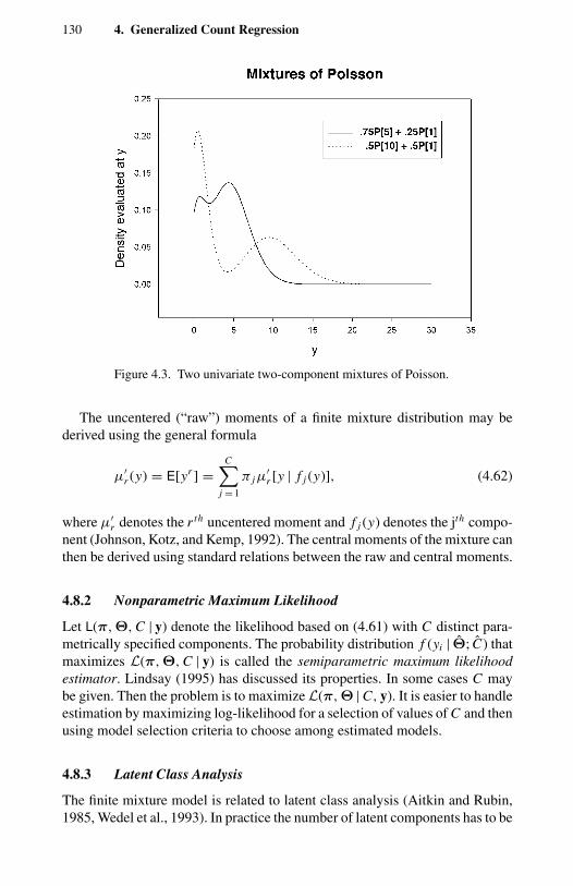
130 4. Generalized Count Regression

Figure 4.3. Two univariate two-component mixtures of Poisson.

The uncentered (“raw”) moments of a finite mixture distribution may bederived using the general formula

µ′r (y) = E[yr ] =

C∑j = 1

π jµ′r [y | f j (y)], (4.62)

where µ′r denotes the r th uncentered moment and f j (y) denotes the jth compo-

nent (Johnson, Kotz, and Kemp, 1992). The central moments of the mixture canthen be derived using standard relations between the raw and central moments.

4.8.2 Nonparametric Maximum Likelihood

Let L(π,Θ, C | y) denote the likelihood based on (4.61) with C distinct para-metrically specified components. The probability distribution f (yi | Θ; C) thatmaximizes L(π,Θ, C | y) is called the semiparametric maximum likelihoodestimator. Lindsay (1995) has discussed its properties. In some cases C maybe given. Then the problem is to maximize L(π,Θ | C, y). It is easier to handleestimation by maximizing log-likelihood for a selection of values of C and thenusing model selection criteria to choose among estimated models.

4.8.3 Latent Class Analysis

The finite mixture model is related to latent class analysis (Aitkin and Rubin,1985, Wedel et al., 1993). In practice the number of latent components has to be

4.8. Finite Mixtures and Latent Class Analysis 131

estimated, but initially we assume that the number of components in the mixture,C , is given. Let di = (di1, . . . , diC ) define an indicator (dummy) variable suchthat di j = 1;

∑j di j = 1, indicating that yi was drawn from the j th (latent) group

or class for i = 1, . . . , n. That is, each observation may be regarded as a drawfrom one of the C latent classes or “types,” each with its own distribution. Thefinite mixture model specifies that (yi | di ,θ,π) are independently distributedwith densities

C∑j = 1

di j f (yi |θ j ) =C∏

j=1

f (yi |θ j )di j,

and (di j | θ,π) are iid with multinomial distribution

C∏j = 1 j

πdi j

j , 0 < π j < 1,

C∑j = 1

π j = 1.

The last two relations imply that

(yi |θ,π)iid∼

C∑j = 1

πdi j

j f j (y;θ j ), 0 < π j < 1,

C∑j = 1

π j = 1,

where π′ = [π1, . . . , πC ] and θ= [θ1, . . . ,θC ]. Hence the likelihood functionis

L(θ,π | y) =n∏

i = 1

C∑j = 1

πdi j

j [ f j (y;θ j )]di j , 0 < π j < 1,

C∑j = 1

π j = 1.

(4.63)

If π j , j = 1, . . . , C , is given, the posterior probability that observation yi

belongs to the population j , j = 1, 2, . . . , C , denoted zi j , is given by

zi j ≡ Pr[yi ∈ population j] = π j f j(yi | x′

i ,θ j)∑C

j = 1 π j f j(yi | x′

i ,θ j) . (4.64)

The average value of zi j over i is the probability that a randomly chosen indi-vidual belongs to subpopulation j . This equals π j :

E[zi j ] = π j .

4.8.4 Estimation

A widely recommended procedure for estimating the finite mixture model isthe EM procedure, which is structured as follows. Given an initial estimate[π(0),θ(0)], the likelihood function (4.63) may be maximized directly or using

132 4. Generalized Count Regression

the EM algorithm in which the variables di j are treated as missing data. If thedi j were observable the log-likelihood of the model would be

L(π,Θ | y) =n∑

i = 1

C∑j = 1

di j [ln f j (yi ;θ j ) + ln π j ]. (4.65)

Replacing di j by its expected value, E[di j ], yields the expected log-likelihood,

EL(Θ | y,π) =n∑

i = 1

C∑j = 1

zi j [ln f j (yi ;θ j ) + ln π j ], (4.66)

where

E[di j ] = zi j .

The M step of the EM procedure maximizes (4.66) by solving the first-orderconditions

π j −∑n

i = 1 zi j

n= 0, j = 1, . . , C (4.67)

n∑i = 1

C∑j = 1

zi j∂ ln f j (yi ;θ j )

∂θ j= 0. (4.68)

The marginal probability that an observation comes from the subpopulation jis the average of all individual observation probabilities of coming from the j th

population. The E step of the EM procedure obtains new values of E[di j ] using(4.64).

The EM algorithm may be slow to converge, especially if the starting val-ues are not good. Other approaches such as the Newton-Raphson or Broyden-Fletcher-Goldfarb-Shanno may also be worth considering. A discussion of re-liable algorithms is in Bohning (1995). The applications reported in Chapter 6use Newton-Raphson with numerically estimated gradients.

For C given, the covariance matrix of estimated parameters is obtained byspecializing the results in section 2.3.2. Alternative estimators for the variance,including the sandwich and robust sandwich estimators, are also available.However, these should be used with caution, especially if C is likely to bemisspecified. Treating C as known, if in fact it is not, means that the estimatedvariances are conditional quantities.

4.8.5 Inference on C

The preceding account has not dealt with the choice of the parameter C . Twoapproaches have been widely considered in the literature. The first is to uselikelihood ratio to test C = C∗ versus C = C∗ + 1. This is equivalent to the testof H0 : πC∗+1 = 0 versus H1 : πC∗+1 = 0. Unfortunately, the likelihood ratio

4.8. Finite Mixtures and Latent Class Analysis 133

test statistic in this case does not have the standard chi-squared distributionbecause the regularity conditions for likelihood-based inference are violated.

For example, let C = 2. We wish to test

H0 : f (yi |Θ) = P[θ1]

against

H1 : f (yi |Θ) = (1 − π ) P[θ1] + πP[θ2].

where Θ = (π,θ1,θ2) ∈ [0, 1] × (0, ∞) × (0, ∞), where θ1 = θ2. The nullholds if either π = 0 or θ1 = θ2. That is, the parameter space where H0 holdsis

Θ0 = (π,θ) = [0] × (0, ∞) × (0, ∞) ∪ [0, 1] × (0, ∞),

where θ1 =θ2 =θ. This is the entire θ space if π = 0, and the line segment[0, 1] if θ1 =θ2. Under the null hypothesis the parameter π is not identifiablebecause it is on the boundary of the parameter space. The standard assumptionfor likelihood-based testing assumes regularity conditions stated in section 2.3.This includes the condition that Θ is in the interior of parameter space. Hence,the standard asymptotic distribution theory does not apply. Specifically, thelikelihood ratio test statistic does not have the chi-squared distribution underthe null. Hence, the standard critical values are inappropriate. One solution tothis problem is to use a parametric bootstrap to obtain the critical values (Fengand McCulloch, 1996; see also section 6.4). This computer-intensive techniquehas not been widely used in the Poisson regression context.

A second, simpler approach is to first fix the largest value of C one is preparedto accept. Often this is a small number like 2, 3, or 4. The model is estimated forall values of C ≤ C∗. Information criteria are used to select C (see Chapter 5).Chapter 6 contains examples and further discussion.

In an unconstrained model, adding additional components can easily leadto overparameterization in two senses. The total number of parameters maybe large. Then the number of components may also be too large relative tothe information in the data. Because the problem is akin to classification into“types,” doing so reliably requires that interindividual differences are largein the relevant sense. In the case of a constrained mixture, such as the ran-dom intercept model, the resulting increase in the number of parameters issmall, but in the unconstrained model in which all parameters are allowed tovary, the total number of parameters can be quite large (see Chapter 6 for anexample).

If the model is overparameterized, one can expect difficulties in estimationdue to flat log-likelihood. This problem is further compounded by the possiblemultimodality of the mixture likelihood. Thus it is possible for an estimationalgorithm to converge to a local rather than a global maximum. In practicalapplications of finite mixtures, therefore, it is important to test for the presenceof mixture components. If the evidence for mixture is weak, identification is a

134 4. Generalized Count Regression

problem. It is also important to test whether a global maximum of the likelihoodis attained. These important issues are reconsidered in Chapter 6.

4.9 Estimation by Simulation

The specific parametric models of heterogeneity considered in this chapter havethe convenient feature that they generate a closed-form marginal distribution,which then forms the basis of the likelihood. Such an outcome is somewhat arti-ficially generated. In many otherwise appealing models a closed-form marginaldensity may not be generated. It is still possible to estimate the parameters of themixture distribution using computer-intensive methods such as simulated max-imum likelihood or simulated method of moments (Gourieroux and Monfort,1997). The approach is illustrated using a Poisson–normal mixture.

Consider the Poisson model with normally distributed multiplicative hetero-geneity term

yi | µi , νi ∼ P[yi | exp

(x′

iβ + σνi)]

,

νi ∼ N[0, 1].

The marginal distribution is

h(yi | µi )=Eν

[f[yi | exp

(x′

iβ + σνi)]]

=∫ ∞

−∞f[yi | exp

(x′

iβ + σνi)]

φ(νi ) dνi

=∫ ∞

−∞

1

yi !exp(−exp

[x′

iβ + σνi])

× exp[(

x′iβ + σνi

)yi] 1√

2πe−ν2/2 dνi , (4.69)

where the third line follows because φ(ν) is the standard normal density. Thereis no closed-form solution for h(yi | µi ), unlike for the gamma heterogeneityterm considered in section 4.2.

An alternative approach is to use simulation. Because the marginal distri-bution is a mathematical expectation, the expression can be approximated byreplacing the n-element vector ν by draws from the N[0, 1] distribution. Then

h(yi | µi ) ≈ 1

S

S∑s = 1

f[yi | exp

(x′

iβ + σν(s)i

)]. (4.70)

This method is also called Monte Carlo integration. The simulated likelihoodfunction can be built up using n terms like that above. To intuitively understandthe procedure note that if the heterogenenity term were observable then thelikelihood could be constructed directly. In the absence of such information,

4.10. Derivations 135

we use S draws from a pseudorandom number generator to approximate theterm. Simulated maximum likelihood estimates are obtained by maximizingthe log-likelihood function

L(β, σ ) =n∑

i = 1

ln1

S

S∑s = 1

f[yi | exp

(x′

iβ + σν(s)i

)]. (4.71)

It is known that if S is held fixed while n → ∞, the resulting estimator of(β, σ ) is biased (McFadden and Ruud, 1994; Gourieroux and Monfort, 1997).However, if S and n tend to infinity in such a way that

√S/n → 0, the estimator

is both consistent and asymptotically efficient. An active area of research, forproblems in which it is computationally burdensome to let S go to infinity, isto incorporate a bias correction in the expression for the density and then buildthe likelihood from it. For relatively simple problems such as this example,however, there is no need to do this, as there is no practical problem in using avery high value of S.

An alternative estimation procedure may be based on numerical integra-tion. Here the integration is replaced by an H -point Gaussian quadrature withquadrature points (nodes) νh and weights wh ,

h(yi | µi ) ≈ 1√π

H∑h = 1

wh[ f [yi | µi , νh]].

This approach was used by Hinde (1982) for Poisson-normal model. The tableof weights for Gaussian quadrature can be found in Stroud and Secrest (1966).

The simulation approach is flexible and potentially very useful in the contextof truncated or censored models with unobserved heterogeneity and also struc-tural models. An example is given in Chapter 11. The simulation approach isnow also widely used in Bayesian analyses of posterior distributions that maynot possess a closed form.

4.10 Derivations

We sketch a proof of the Two Crossings Theorem, following Shaked (1980).For simplicity, we consider only a one-parameter exponential family, whichcovers distributions other than the Poisson, which is of main interest here.

For the random variable y, y ∈ Ry , let

f (y; θ ) = expa(θ ) + c(θ )y

denote the density. We consider mixing with respect to θ , θ ∈ Rθ , given π (θ ),a nondegenerate distribution with mean

µ =∫

Rθ

θπ (θ ) dθ.

136 4. Generalized Count Regression

The mixture density,

h(y) =∫

Rθ

expa(θ) + c(θ )yπ (θ ) dθ,

is approximated by

f (y) ≡ f (y | µ) = expa(µ) + c(µ)y,obtained by replacing θ by its mean µ in f (y; θ ). The Two Crossings Theoremstudies the sign pattern of h(y)− f (y), assuming that the parent and the mixturedistributions have the same mean; that is,∫

y f (y | µ) dy =∫

yh(y) dy. (4.72)

Let S−(h − f ) denote the number of sign changes in h − y over the set R(y).The number of sign changes of h − f is the same as the number of sign changesof the function

r (y)= h(y)

f (y)− 1

=∫

R(θ )exp(a(θ ) − a(µ)) + (c(θ ) − c(µ))yπ (θ ) dθ − 1.

Because r (y) is convex on the setRy it is implied that S−(h− f ) ≤ 2. ObviouslyS−(h − f ) = 0. To show that S−(h − f ) = 1, assume, on the contrary thatS−(h − f ) = 1. If the sign sequence is +, − then the cdf H (y) = ∫ h(y) dyand F(y) = ∫ f (y) dy satisfy

F(y) ≥ H (y)

for all y. This result, together with h = f , implies∫yh(y) dy <

∫y f (y) dy,

which contradicts the assumption of equal means, (4.72). Similarly if the se-quence is −, +, (4.72) is also contradicted. Thus S−(h − f ) = 1 and henceS−(h− f ) = 2. The sign sequence +, −, + follows from the convexity of r (y).

4.11 Bibliographic Notes

Feller (1971) is a classic reference for several topics discussed in this chapter.Cox processes are concisely discussed in Kingman (1993, pp. 65–72). A re-cent accessible discussion of the Two Crossings Theorem of Shaked (1980) isby Mullahy (1997b). Shaked’s analysis applies to a one-parameter exponentialfamily. The two-crossings result is extended by Gelfand and Dalal (1990, p. 57)to a two-parameter exponential family by exploiting convexity as in section 8.9.

4.12. Exercises 137

Chapters 4 and 5 in Lancaster (1990) contain material complementary to that insections 4.2 and 4.3. Our material in section 2.3.5 borrows heavily from Winkel-mann (1995), who provides a useful discussion of dependence and dispersion.Lee (1997) provides a further development and important extensions of thisapproach using simulated maximum likelihood to estimate the model. Gourier-oux and Visser (1997) also use the duration model to define a count model; theyalso consider the heterogeneity distribution arising from the presence of bothindividual and spell-specific components.

Lucerno (1995) examines several models in which clustering leads to overdis-persion. An application of truncated Poisson is Grogger and Carson (1991).See also Creel and Loomis (1990) and Brannas (1992). The monograph byMcLachlan and Basford (1988) provides a good treatment of finite mixtures,and Wedel et al. (1993) and Deb and Trivedi (1997) are econometric applica-tions. Brannas and Rosenqvist (1994) and Bohning (1995) have outlined thecomputational properties of alternative algorithms. Finite mixtures can be han-dled in a Bayesian framework using Markov chain Monte Carlo methods as inRobert (1996). Detailed analysis of the moment properties of truncated countregression models include Gurmu (1991), who considers the zero-truncatedPoisson, and Gurmu and Trivedi (1992), who deal with left or right trunca-tion in general and who also deal with tests of overdispersion in the truncatedPoisson regression. Censored Poisson regression was analyzed in some detailby Gurmu (1993), who uses the EM algorithm. Amemiya (1985) provides agood exposition of the EM algorithm. Crepon and Duguet (1997b) apply thesimulation-based estimator to a panel model. Treatment of heterogeneity basedon simulation is quite general in Gourieroux and Monfort (1991). A flexible ap-proach to count models based on series expansions is given later in Chapter 12,which also gives further references. Some background material for this is inChapter 8.

4.12 Exercises

4.1 The Katz family of distributions is defined by the probability recursion

Pr[y + 1]

Pr[y]= µ + γ y

1 + yfor y = 0, 1, . . . , and µ + γ y ≥ 0.

Show that this yields overdispersed distributions for 0 < γ < 1, and underdis-persed distributions for γ < 0.

4.2 Using the NB2 density show that the density collapses to that of the Poissonas the variance of the mixing distribution approaches zero.

4.3 The Poisson-lognormal mixture is obtained by considering the followingmodel in which µ is normally distributed with mean x′β and variance 1. That is,given y | µν ∼ P[µν], ln µν = x′β+ σν, ν ∼ N[0, 1], show that although thePoisson-lognormal mixture cannot be written in a closed form, the mean of themixture distribution is shifted by a constant. Show that the first two moments

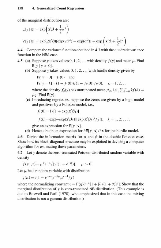
138 4. Generalized Count Regression

of the marginal distribution are:

E[y | x] = exp

(x′β + 1

2σ 2

)V[y | x] = exp(2x′β)[exp(2σ 2) − exp(σ 2)] + exp

(x′β + 1

2σ 2

).

4.4 Compare the variance function obtained in 4.3 with the quadratic variancefunction in the NB2 case.

4.5 (a) Suppose y takes values 0, 1, 2, . . . with density f (y) and mean µ. FindE[y | y > 0].

(b) Suppose y takes values 0, 1, 2, . . . with hurdle density given by

Pr[y = 0]= f1(0) and

Pr[y = k]= (1 − f1(0))/(1 − f2(0)) f2(0), k = 1, 2, . . .

where the density f2(y) has untruncated mean µ2, i.e.,∑∞

k = 0 k f (k) =µ2. Find E[y].

(c) Introducing regressors, suppose the zeros are given by a logit modeland positives by a Poisson model, i.e.,

f1(0)=1/[1 + exp(x′β1)]

f (k)=exp[−exp(x′β2)][exp(x′β2)k/y!], k = 1, 2, . . . ;

give an expression for E[y | x].(d) Hence obtain an expression for ∂E[y | x]/∂x for the hurdle model.

4.6 Derive the information matrix for µ and φ in the double-Poisson case.Show how its block-diagonal structure may be exploited in devising a computeralgorithm for estimating these parameters.

4.7 Let y denote the zero-truncated Poisson-distributed random variable withdensity

f (y | µ) = µye−µ/[y!(1 − e−µ)], µ > 0.

Let µ be a random variable with distribution

g(µ) = c(1 − e−µ)e−θµµη−1/y!

where the normalizing constant c = (η)θ−η[1 + [θ/(1 + θ )]η]. Show that themarginal distribution of y is zero-truncated NB distribution. (This example isdue to Boswell and Patil (1970), who emphasized that in this case the mixingdistribution is not a gamma distribution.)

CHAPTER 5

Model Evaluation and Testing

5.1 Introduction

It is desirable to analyze count data using a cycle of model specification, es-timation, testing, and evaluation. This cycle can go from specific to generalmodels – for example, it can begin with Poisson and then test for negative bino-mial – or one can use a general to specific approach – for example, begin withnegative binomial and then test the restrictions imposed by Poisson. For inclu-sion of regressors in a given count model either approach might be taken; forchoice of the count data model itself other than simple choices such as Poissonor negative binomial the former approach is most often useful. For example, ifthe negative binomial model is inadequate, there is a very wide range of modelsthat might be considered, rendering a general-to-specific approach difficult toimplement.

The preceding two chapters have presented the specification and estimationcomponents of this cycle for cross-section count data. In this chapter we focus onthe testing and evaluation aspects of this cycle. This includes residual analysis,goodness-of-fit measures, and moment-based specification tests, in addition toclassical statistical inference.

Residual analysis, based on a range of definitions of the residual for het-eroskedastic data such as counts, is presented in section 5.2. A range of measuresof goodness of fit, including pseudo R-squareds and a chi-square goodness-of-fit statistic, are presented in section 5.3. Likelihood-based hypothesis testsfor overdispersion, introduced in section 3.4, are discussed more extensivelyin section 5.4. Small-sample corrections, including the bootstrap pairs proce-dure for quite general cross-section data models, are presented in section 5.5.Moment-based tests, using the conditional moment test framework, are pre-sented in section 5.6. Discrimination among nonnested models is the subject ofsection 5.7. Many of the methods are illustrated using a regression model forthe number of takeover bids, which is introduced in section 5.2.5.

The presentation here is in places very detailed. For the practitioner, theuse of simple residuals such as Pearson residuals is well-established and canbe quite informative. For overall model fit in fully parametric models, chi-square goodness-of-fit measures are straightforward to implement. In testing

140 5. Model Evaluation and Testing

for overdispersion in the Poisson model, the overdispersion tests presentedalready in section 3.4 often are adequate. The current chapter gives a moretheoretical treatment. Bootstrap methods, such as those outlined here, shouldbe performed if more refined small-sample inference is desired. Conditionalmoment tests are easily implemented, but their interpretation if they are appliedto count data is quite subtle due to the inherent heteroskedasticity. Finally,the standard methods for discriminating between nonnested models have beenadapted to count data.

The treatment of many of these topics, as with estimation, varies according towhether we use a fully parametric maximum likelihood framework or a condi-tional moment approach based on specification of the first one or two momentsof the dependent variable. Even within this classification results may be spe-cialized, notably maximum likelihood methods to LEF and moment methodsto GLMs. Also, most detailed analysis is restricted to cross-section data. Manyof the techniques presented here have been developed only for such specialcases and their generality is not always clear. There is considerable scope forgeneralization and application to a broader range of count data models.

5.2 Residual Analysis

Residuals measure the departure of fitted values from actual values of the de-pendent variable. They can be used to detect model misspecification; to detectoutliers, or observations with poor fit; and to detect influential observations, orobservations with a big impact on the fitted model.

Residual analysis, particularly visual analysis, can potentially indicate thenature of misspecification and ways that it may be corrected, as well as providea feel for the magnitude of the effect of the misspecification. By contrast, formalstatistical tests of model misspecification can be black boxes, producing only asingle number that is then compared to a critical value. Moreover, if one testsat the same significance level (usually 5%) without regard to sample size, anymodel using real data will be rejected with a sufficiently large sample even if itdoes fit the data well.

For linear models a residual is easily defined as the difference betweenactual and fitted value. For nonlinear models the very definition of a residualis not unique. Several residuals have been proposed for the Poisson and otherGLMs. These residuals do not always generalize in the presence of commoncomplications, such as censored or hurdle models, for which it may be morefruitful to appeal to residuals proposed in the duration literature. We presentmany candidate definitions of residuals and stress that at this stage there appearsto be no one single residual that can be used in all contexts.

We also give a brief treatment of detection of outliers and influential ob-servations. This topic is less important in applications in which data sets arelarge and the relative importance of individual observations is small. And ifdata sets are small and an influential or outlying observation is detected, it isnot always clear how one should proceed. Dropping the observation or adapting

5.2. Residual Analysis 141

the model simply to better fit one observation creates concerns of data-miningand overfitting.

5.2.1 Pearson, Deviance, and Anscombe Residuals

The natural residual is the raw residual

ri = (yi − µi ), (5.1)

where the fitted mean µi is the conditional mean µi = µ(x′iβ) evaluated at β =

β. Asymptotically this residual behaves as (yi − µi ), because βp→ β implies

µip→ µi . For the classical linear regression model with normally distributed

homoskedastic error (y − µ) ∼ N[0, σ 2], so that in large samples the rawresidual has the desirable properties of being symmetrically distributed aroundzero with constant variance. For count data, however, (y −µ) is heteroskedasticand asymmetric. For example, if y ∼ P[µ] then (y − µ) has variance µ andthird moment µ. So the raw residual even in large samples is heteroskedasticand asymmetric.

For count data there is no one residual that has zero mean, constant variance,and symmetric distribution. This leads to several different residuals accordingto which of these properties is felt to be most desirable.

The obvious correction for heteroskedasticity is the Pearson residual

pi = (yi − µi )√ωi

, (5.2)

where ωi is an estimate of the variance ωi of yi . The sum of the squares ofthese residuals is the Pearson statistic, defined in (5.16). For the Poisson, GLM,and NB2 models, respectively, one uses ω = µ, ω = αµ and ω = µ + αµ2. Inlarge samples this residual has zero mean and is homoskedastic (with varianceunity), but it is asymmetrically distributed. For example, if y is Poisson thenE[(y − µ)3/

õ] = 1/

õ.

If y is generated by an LEF density one can use the deviance residual, whichis

di = sign (yi − µi )√

2l(yi ) − l(µi ), (5.3)

where l(µ) is the log-density of y evaluated at µ = µ and l(y) is the log-densityevaluated at µ = y. A motivation for the deviance residual is that the sum ofsquares of these residuals is the deviance statistic, defined in (5.18), which is thegeneralization for LEF models of the sum of raw residuals in the linear model.Thus, for the normal distribution with σ 2 known, di = (yi − µi )/σ , the usualstandardized residual. For the Poisson this residual equals

di = sign (yi − µi )√

2yi ln(yi/µi ) − (yi − µi ), (5.4)

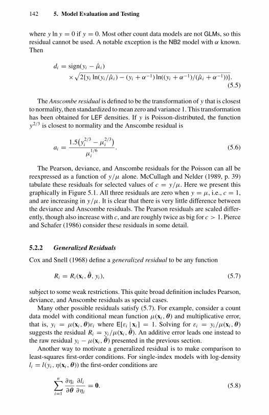
142 5. Model Evaluation and Testing

where y ln y = 0 if y = 0. Most other count data models are not GLMs, so thisresidual cannot be used. A notable exception is the NB2 model with α known.Then

di = sign(yi − µi )

×√

2yi ln(yi/µi ) − (yi + α−1) ln((yi + α−1)/(µi + α−1)).(5.5)

The Anscombe residual is defined to be the transformation of y that is closestto normality, then standardized to mean zero and variance 1. This transformationhas been obtained for LEF densities. If y is Poisson-distributed, the functiony2/3 is closest to normality and the Anscombe residual is

ai = 1.5(y2/3

i − µ2/3i

)µ

1/6i

. (5.6)

The Pearson, deviance, and Anscombe residuals for the Poisson can all bereexpressed as a function of y/µ alone. McCullagh and Nelder (1989, p. 39)tabulate these residuals for selected values of c = y/µ. Here we present thisgraphically in Figure 5.1. All three residuals are zero when y = µ, i.e., c = 1,and are increasing in y/µ. It is clear that there is very little difference betweenthe deviance and Anscombe residuals. The Pearson residuals are scaled differ-ently, though also increase with c, and are roughly twice as big for c > 1. Pierceand Schafer (1986) consider these residuals in some detail.

5.2.2 Generalized Residuals

Cox and Snell (1968) define a generalized residual to be any function

Ri = Ri (xi , θ, yi ), (5.7)

subject to some weak restrictions. This quite broad definition includes Pearson,deviance, and Anscombe residuals as special cases.

Many other possible residuals satisfy (5.7). For example, consider a countdata model with conditional mean function µ(xi ,θ) and multiplicative error,that is, yi = µ(xi ,θ)εi where E[εi | xi ] = 1. Solving for εi = yi/µ(xi ,θ)suggests the residual Ri = yi/µ(xi , θ). An additive error leads one instead tothe raw residual yi − µ(xi , θ) presented in the previous section.

Another way to motivate a generalized residual is to make comparison toleast-squares first-order conditions. For single-index models with log-densityli = l(yi , η(xi ,θ)) the first-order conditions are

n∑i=1

∂ηi

∂θ

∂li

∂ηi= 0. (5.8)

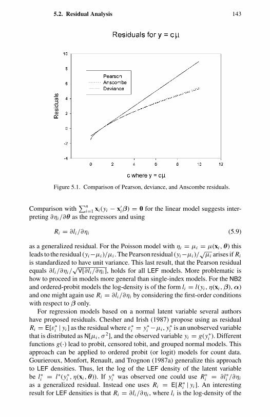
5.2. Residual Analysis 143

Figure 5.1. Comparison of Pearson, deviance, and Anscombe residuals.

Comparison with∑n

i=1 xi (yi − x′iβ) = 0 for the linear model suggests inter-

preting ∂ηi/∂θ as the regressors and using

Ri = ∂li/∂ηi (5.9)

as a generalized residual. For the Poisson model with ηi = µi = µ(xi ,θ) thisleads to the residual (yi −µi )/µi . The Pearson residual (yi −µi )/

õi arises if Ri

is standardized to have unit variance. This last result, that the Pearson residualequals ∂li/∂ηi/

√V[∂li/∂ηi ], holds for all LEF models. More problematic is

how to proceed in models more general than single-index models. For the NB2and ordered-probit models the log-density is of the form li = l(yi , η(xi ,β),α)and one might again use Ri = ∂li/∂ηi by considering the first-order conditionswith respect to β only.

For regression models based on a normal latent variable several authorshave proposed residuals. Chesher and Irish (1987) propose using as residualRi = E[ε∗

i | yi ] as the residual where ε∗i = y∗

i −µi , y∗i is an unobserved variable

that is distributed as N[µi , σ2], and the observed variable yi = g(y∗

i ). Differentfunctions g(·) lead to probit, censored tobit, and grouped normal models. Thisapproach can be applied to ordered probit (or logit) models for count data.Gourieroux, Monfort, Renault, and Trognon (1987a) generalize this approachto LEF densities. Thus, let the log of the LEF density of the latent variablebe l∗i = l∗(y∗

i , η(xi ,θ)). If y∗i was observed one could use R∗

i = ∂l∗i /∂ηi

as a generalized residual. Instead one uses Ri = E[R∗i | yi ]. An interesting

result for LEF densities is that Ri = ∂li/∂ηi , where li is the log-density of the

144 5. Model Evaluation and Testing

observed variable. Thus the same residual is obtained by applying (5.9) to thelatent variable model and then conditioning on observed data as is obtained bydirectly applying (5.9) to the observed variable.

A count application is the left-truncated Poisson model, studied by Gurmuand Trivedi (1992), whose results were summarized in section 4.5. Then y∗

i ∼P[µi ] and we observe yi = y∗

i if y∗i ≥ r . For the latent variable model R∗

i =(y∗

i −µi )/µi . Because E[y∗i | y∗

i ≥ r ] = µi +δi , where the correction factor δi isgiven in section 4.5.1, the residual for the observed variable is Ri = E[R∗

i | y∗i ≥

r ] = (yi − µi − δi )/µi . Alternatively, inspection of the maximum-likelihoodfirst-order conditions given in section 4.5.2 also leads to this residual.

5.2.3 Using Residuals

Perhaps the most fruitful way to use residuals is by plotting residuals againstother variables of interest. Such plots include residuals plotted against predictedvalues of the dependent variable, for example to see whether the fit is poor forsmall or large values of the dependent variable; against omitted regressors, tosee whether there is any relationship in which case the residuals should beincluded; and against included regressors, to see whether regressors shouldenter through a different functional form than that specified.

For the first plot it is tempting to plot residuals against the actual value ofthe dependent variable, but such a plot is not informative for count data. To seethis, consider this plot using the raw residual. Because Cov[y − µ, y] = V[y],which equals µ for Poisson data, there is a positive relationship between y − µ

and y. Such plots are more useful for the linear regression model under clas-sical assumptions, in which case V[y] is a constant and any pattern in therelationship between y − µ and y is interpreted as indicating heteroscedas-ticity. For counts we instead plot residuals against predicted means and notethat Cov[y − µ, µ] = 0. A variation is to plot the actual value of y againstthe predicted value. This plot is difficult to interpret, however, if the dependentvariable takes only a few values.

If there is little variation in predicted means the residuals may also be lumpydue to lumpiness in y, making plots of the residuals against the fitted mean dif-ficult to interpret. A similar problem arises in the logit and other discrete choicemodels. Landwehr, Pregibon, and Shoemaker (1984) propose graphical smooth-ing methods (see also Chesher and Irish, 1987). For the probit model based ona normal latent variable, Gourieroux, Monfort, Renault, and Trognon (1987b)propose use of simulated residuals as a way to overcome lumpiness, but thisadds considerable noise. The approach could be applied to ordered probit andlogit models for count data for which the underlying latent variable is discrete.

Even if the variables being plotted are not lumpy it can still be difficult todetect a relationship, and it is preferable to perform a nonparametric regressionof R on x , where R denotes the residual being analyzed and x is the variable itis being plotted against. One can then plot the predictions R against x , whereR is the estimate of the potentially nonlinear mean E[R | x].

5.2. Residual Analysis 145

There are a number of methods for such nonparametric regression. Let yi bea dependent variable, in the preceding discussion a model residual, and xi bea regressor, in the preceding discussion the dependent variable, fitted mean, ormodel regressor. We wish to estimate E[yl | xl], where the evaluation points xl

may or may not be actual sample values of x . The nonparametric estimator ofthe regression function is

yl = E[yl | xl] =(

n∑i=1

wil yi

)/(n∑

i=1

wil

)(5.10)

where the weights wil are decreasing functions of |xi − xl |. Different methodslead to different weighting functions, with kernel and nearest-neighbors meth-ods particularly popular. A more recent method that is easy to implement andappears to perform well is weighted local linear regression, proposed by Fan(1992).

An overall test of adequacy of a model may be to see how close the residualsare to normality. This can be done by a normal scores plot, which orders theresiduals ri from smallest to largest and plots them against the values predictedif the residuals were exactly normally distributed, that is, plot the ordered ri

against

rnormi = r + sr −1((i − .5)/n), (5.11)

i = 1, . . . , n, where sr is the sample standard deviation of r and −1 is theinverse of the standard normal cdf. If the residuals are exactly normal thisproduces a straight line. Davison and Gigli (1989) advocate using such normalscores plots with deviance residuals to check distributional assumptions.

5.2.4 Small Sample Corrections and Influential Observations

The preceding motivations for the various residuals have implicitly treated µi asµi , ignoring estimation error in µi . Estimation error can lead to quite differentsmall-sample behavior between, for example, the raw residual (yi − µi ) and(yi − µi ) just as it does in the linear regression model.

In the linear model, y = x′iβ+u, it is a standard result that the OLS residual

vector (y−µ) = (I − H)u, where H = X(X′X)−1X′. Under classic assumptionsthat E[uu′] = σ 2I it follows that E[(y − µ)(y − µ)′] = σ 2(I − H). Therefore,(yi − µi ) has variance (1 − hii )σ 2, where hii is the i th diagonal entry of H. Forvery large n, hii → 0 so the OLS residual has variance σ 2 as expected. But forsmall n the variance may be quite different and it is best to use the standardizedresidual (yi − µi )/

√(1 − hii )s2.

The matrix H also appears in detecting influential observations. Because inthe linear model µ = y = Hy, H is called the hat matrix. If hii , the i th diagonalentry in H, is large, then the design matrix X, which determines H, is such thatyi has a big influence on its own prediction.

146 5. Model Evaluation and Testing

Pregibon (1981) generalized this analysis to the logit model. The logit resultsin turn have been extended to GLMs (see for example Williams, 1987, andMcCullagh and Nelder, 1989 for a summary). For GLMs the hat matrix is

H = W1/2X(X′WX)−1X′W1/2, (5.12)

where W = Diag[wi ], a diagonal matrix with i th entry wi , and wi = (∂µi/

∂x′iβ)2/V[yi ]. For the Poisson with exponential mean function wi = µi , so

H is easily calculated. As in the linear model the n × n matrix H is idempotentwith trace equal to its rank k, the number of regressors. So the average valueof hii is k/n, and values of hii in excess of 2k/n are viewed as having highleverage. The studentized Pearson residual is

p∗i = pi/

√1 − hii (5.13)

and the studentized deviance residual is

d∗i = di/

√1 − hii . (5.14)

Other small-sample corrections for generalized residuals are given by Cox andSnell (1968). See also Davison and Snell (1991), who consider GLM and moregeneral residuals.

A practical problem in implementing these methods is that H is of dimensionn × n, so that if one uses the obvious matrix commands to compute H the dataset cannot be too large, due to the need to compute a matrix with n2 elements.Even n = 100 may lead to problems in some programs that support matrixcommands, and some ingenuity may be needed to calculate the diagonal entriesin H.

These asymptotic approximations are for small n. Some authors also con-sider so-called small-m asymptotics, which correct for not having multipleobservations on y for each value of the regressors. Such corrections lead toan adjusted deviance residual that is closer to the normal distribution than thedeviance residual. For the Poisson the adjusted deviance residual is

dadji = di + 1/(6√

µi ). (5.15)

Pierce and Schafer (1986) find that the adjusted deviance residual is closestto normality, after taking account of the discreteness by making a continuitycorrection that adds or subtracts 0.5 to or from y, toward the center of thedistribution.

5.2.5 Example: Takeover Bids

Jaggia and Thosar (1993) model the number of bids received by 126 U.S. firmsthat were targets of tender offers during the period from 1978 through 1985 andwere actually taken over within 52 weeks of the initial offer. The dependent

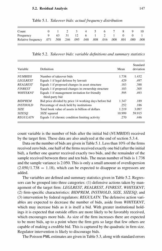
5.2. Residual Analysis 147

Table 5.1. Takeover bids: actual frequency distribution

Count 0 1 2 3 4 5 6 7 8 9 10Frequency 9 63 31 12 6 1 2 1 0 0 1Relative frequency .071 .500 .246 .095 .048 .008 .016 .008 .001 .000 .008

Table 5.2. Takeover bids: variable definitions and summary statistics

StandardVariable Definition Mean deviation

NUMBIDS Number of takeover bids 1.738 1.432LEGLREST Equals 1 if legal defense by lawsuit .429 .497REALREST Equals 1 if proposed changes in asset structure .183 .388FINREST Equals 1 if proposed changes in ownership structure .103 .305WHITEKNT Equals 1 if management invitation for friendly .595 .493

third-party bidBIDPREM Bid price divided by price 14 working days before bid 1.347 .189INSTHOLD Percentage of stock held by institutions .252 .186SIZE Total book value of assets in billion of dollars 1.219 3.097SIZESQ SIZE squared 10.999 59.915REGULATN Equals 1 if chronic condition limiting activity .270 .446

count variable is the number of bids after the initial bid (NUMBIDS) receivedby the target firm. These data are also analyzed at the end of section 5.3.4.

Data on the number of bids are given in Table 5.1. Less than 10% of the firmsreceived zero bids, one half of the firms received exactly one bid (after the initialbid), a further one quarter received exactly two bids, and the remainder of thesample received between three and ten bids. The mean number of bids is 1.738and the sample variance is 2.050. This is only a small amount of overdispersion(2.050/1.738 = 1.18), which can be expected to disappear as regressors areadded.

The variables are defined and summary statistics given in Table 5.2. Regres-sors can be grouped into three categories: (1) defensive actions taken by man-agement of the target firm: LEGLREST, REALREST, FINREST, WHITEKNT;(2) firm-specific characteristics: BIDPREM, INSTHOLD, SIZE, SIZESQ; and(3) intervention by federal regulators: REGULATN. The defensive action vari-ables are expected to decrease the number of bids, aside from WHITEKNT,which may increase bids as it is itself a bid. With greater institutional hold-ings it is expected that outside offers are more likely to be favorably received,which encourages more bids. As size of the firm increases there are expectedto be more bids, up to a point where the firm gets so large that few others arecapable of making a credible bid. This is captured by the quadratic in firm size.Regulator intervention is likely to discourage bids.

The Poisson PML estimates are given in Table 5.3, along with standard errors

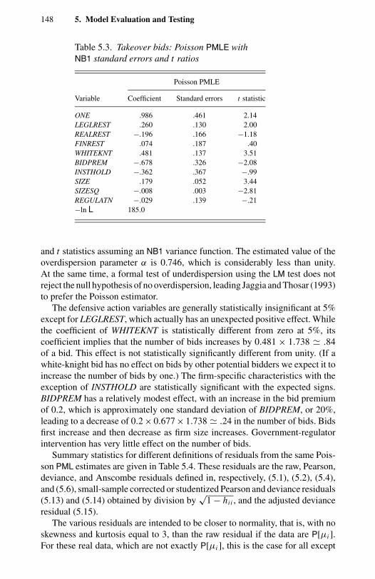
148 5. Model Evaluation and Testing

Table 5.3. Takeover bids: Poisson PMLE withNB1 standard errors and t ratios

Poisson PMLE

Variable Coefficient Standard errors t statistic

ONE .986 .461 2.14LEGLREST .260 .130 2.00REALREST −.196 .166 −1.18FINREST .074 .187 .40WHITEKNT .481 .137 3.51BIDPREM −.678 .326 −2.08INSTHOLD −.362 .367 −.99SIZE .179 .052 3.44SIZESQ −.008 .003 −2.81REGULATN −.029 .139 −.21−ln L 185.0

and t statistics assuming an NB1 variance function. The estimated value of theoverdispersion parameter α is 0.746, which is considerably less than unity.At the same time, a formal test of underdispersion using the LM test does notreject the null hypothesis of no overdispersion, leading Jaggia and Thosar (1993)to prefer the Poisson estimator.

The defensive action variables are generally statistically insignificant at 5%except for LEGLREST, which actually has an unexpected positive effect. Whilethe coefficient of WHITEKNT is statistically different from zero at 5%, itscoefficient implies that the number of bids increases by 0.481 × 1.738 .84of a bid. This effect is not statistically significantly different from unity. (If awhite-knight bid has no effect on bids by other potential bidders we expect it toincrease the number of bids by one.) The firm-specific characteristics with theexception of INSTHOLD are statistically significant with the expected signs.BIDPREM has a relatively modest effect, with an increase in the bid premiumof 0.2, which is approximately one standard deviation of BIDPREM, or 20%,leading to a decrease of 0.2 × 0.677 × 1.738 .24 in the number of bids. Bidsfirst increase and then decrease as firm size increases. Government-regulatorintervention has very little effect on the number of bids.

Summary statistics for different definitions of residuals from the same Pois-son PML estimates are given in Table 5.4. These residuals are the raw, Pearson,deviance, and Anscombe residuals defined in, respectively, (5.1), (5.2), (5.4),and (5.6), small-sample corrected or studentized Pearson and deviance residuals(5.13) and (5.14) obtained by division by

√1 − hii , and the adjusted deviance

residual (5.15).The various residuals are intended to be closer to normality, that is, with no

skewness and kurtosis equal to 3, than the raw residual if the data are P[µi ].For these real data, which are not exactly P[µi ], this is the case for all except

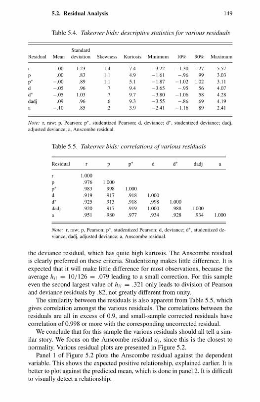
5.2. Residual Analysis 149

Table 5.4. Takeover bids: descriptive statistics for various residuals

StandardResidual Mean deviation Skewness Kurtosis Minimum 10% 90% Maximum

r .00 1.23 1.4 7.4 −3.22 −1.30 1.27 5.57p .00 .83 1.1 4.9 −1.61 −.96 .99 3.03p∗ −.00 .89 1.1 5.1 −1.87 −1.02 1.02 3.11d −.05 .96 .7 9.4 −3.65 −.95 .56 4.07d∗ −.05 1.03 .7 9.7 −3.80 −1.06 .58 4.28dadj .09 .96 .6 9.3 −3.55 −.86 .69 4.19a −.10 .85 .2 3.9 −2.41 −1.16 .89 2.41

Note: r, raw; p, Pearson; p∗, studentized Pearson; d, deviance; d∗, studentized deviance; dadj,adjusted deviance; a, Anscombe residual.

Table 5.5. Takeover bids: correlations of various residuals

Residual r p p∗ d d∗ dadj a

r 1.000p .976 1.000p∗ .983 .998 1.000d .919 .917 .918 1.000d∗ .925 .913 .918 .998 1.000dadj .920 .917 .919 1.000 .988 1.000a .951 .980 .977 .934 .928 .934 1.000

Note: r, raw; p, Pearson; p∗, studentized Pearson; d, deviance; d∗, studentized de-viance; dadj, adjusted deviance; a, Anscombe residual.

the deviance residual, which has quite high kurtosis. The Anscombe residualis clearly preferred on these criteria. Studentizing makes little difference. It isexpected that it will make little difference for most observations, because theaverage hii = 10/126 = .079 leading to a small correction. For this sampleeven the second largest value of hii = .321 only leads to division of Pearsonand deviance residuals by .82, not greatly different from unity.

The similarity between the residuals is also apparent from Table 5.5, whichgives correlation amongst the various residuals. The correlations between theresiduals are all in excess of 0.9, and small-sample corrected residuals havecorrelation of 0.998 or more with the corresponding uncorrected residual.

We conclude that for this sample the various residuals should all tell a sim-ilar story. We focus on the Anscombe residual ai , since this is the closest tonormality. Various residual plots are presented in Figure 5.2.

Panel 1 of Figure 5.2 plots the Anscombe residual against the dependentvariable. This shows the expected positive relationship, explained earlier. It isbetter to plot against the predicted mean, which is done in panel 2. It is difficultto visually detect a relationship.

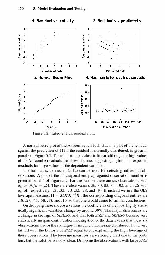
150 5. Model Evaluation and Testing

Figure 5.2. Takeover bids: residual plots.

A normal score plot of the Anscombe residual, that is, a plot of the residualagainst the prediction (5.11) if the residual is normally distributed, is given inpanel 3 of Figure 5.2. The relationship is close to linear, although the high valuesof the Anscombe residuals are above the line, suggesting higher-than-expectedresiduals for large values of the dependent variable.

The hat matrix defined in (5.12) can be used for detecting influential ob-servations. A plot of the i th diagonal entry hii against observation number isgiven in panel 4 of Figure 5.2. For this sample there are six observations withhii > 3k/n = .24. These are observations 36, 80, 83, 85, 102, and 126 withhii of, respectively, .28, .32, .70, .32, .28, and .30. If instead we use the OLSleverage measures, H = X(X′X)−1X′, the corresponding diagonal entries are.18, .27, .45, .58, .18, and .16, so that one would come to similar conclusions.

On dropping these six observations the coefficients of the most highly statis-tically significant variables change by around 30%. The major differences area change in the sign of SIZESQ, and that both SIZE and SIZESQ become verystatistically insignificant. Further investigation of the data reveals that these sixobservations are for the six largest firms, and that the size distribution has a veryfat tail with the kurtosis of SIZE equal to 31, explaining the high leverage ofthese observations. The leverage measures very strongly alert one to the prob-lem, but the solution is not so clear. Dropping the observations with large SIZE

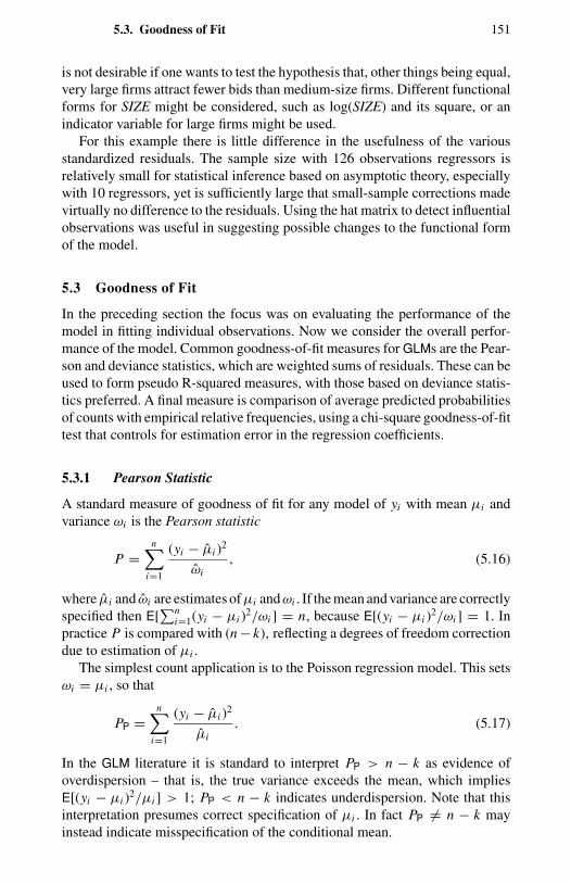
5.3. Goodness of Fit 151

is not desirable if one wants to test the hypothesis that, other things being equal,very large firms attract fewer bids than medium-size firms. Different functionalforms for SIZE might be considered, such as log(SIZE) and its square, or anindicator variable for large firms might be used.

For this example there is little difference in the usefulness of the variousstandardized residuals. The sample size with 126 observations regressors isrelatively small for statistical inference based on asymptotic theory, especiallywith 10 regressors, yet is sufficiently large that small-sample corrections madevirtually no difference to the residuals. Using the hat matrix to detect influentialobservations was useful in suggesting possible changes to the functional formof the model.

5.3 Goodness of Fit

In the preceding section the focus was on evaluating the performance of themodel in fitting individual observations. Now we consider the overall perfor-mance of the model. Common goodness-of-fit measures for GLMs are the Pear-son and deviance statistics, which are weighted sums of residuals. These can beused to form pseudo R-squared measures, with those based on deviance statis-tics preferred. A final measure is comparison of average predicted probabilitiesof counts with empirical relative frequencies, using a chi-square goodness-of-fittest that controls for estimation error in the regression coefficients.

5.3.1 Pearson Statistic

A standard measure of goodness of fit for any model of yi with mean µi andvariance ωi is the Pearson statistic

P =n∑

i=1

(yi − µi )2

ωi, (5.16)

where µi and ωi are estimates ofµi andωi . If the mean and variance are correctlyspecified then E[

∑ni=1(yi − µi )2/ωi ] = n, because E[(yi − µi )2/ωi ] = 1. In

practice P is compared with (n − k), reflecting a degrees of freedom correctiondue to estimation of µi .

The simplest count application is to the Poisson regression model. This setsωi = µi , so that

PP =n∑

i=1

(yi − µi )2

µi. (5.17)

In the GLM literature it is standard to interpret PP > n − k as evidence ofoverdispersion – that is, the true variance exceeds the mean, which impliesE[(yi − µi )2/µi ] > 1; PP < n − k indicates underdispersion. Note that thisinterpretation presumes correct specification of µi . In fact PP = n − k mayinstead indicate misspecification of the conditional mean.

152 5. Model Evaluation and Testing

In practice even the simplest count data models make some correction foroverdispersion. In the GLM literature the variance is a multiple of the mean asin section 3.2.4. Then ωi = φµi where φ = φNB1 = (n − k)−1∑n

i=1(yi −µi )2/µi . But this implies that P always equals (n − k), so P is no longer auseful diagnostic. If instead one uses the NB2 model, ωi = µi + αµ2

i , withα the maximum likelihood estimate of α from section 3.3.1, then P is stilla useful diagnostic. So the Pearson statistic cannot be used to test whetheroverdispersion is adequately modeled in the GLM framework but can be usedif the NB2 MLE is used. Even here, departures of P from (n − k) may actuallyreflect misspecification of the conditional the mean.

Some references to the Pearson statistic suggest that it is asymptotically chi-square distributed, but this is only true in the special case of grouped data withmultiple observations for each µi . McCullagh (1986) gives the distribution inthe more common case of ungrouped data, in which case one needs to accountfor the dependence of µi on β. This distribution can be obtained by appealto the results on CM tests given in section 2.6.3. Thus TP = P ′V−1

P Pa∼ χ2(1),

where the formula for the variance VP is quite cumbersome. For the NB2 modelestimated by maximum likelihood one can use the simpler OPG form of the CMtest. Then an asymptotically equivalent version of TP is n times the uncenteredR2 from auxiliary regression of 1 on the k +2 regressors (yi − µi )2/(µi + αµ2

i ),(yi −µi )/(1+αµi )xi and α−2[ln(1+αµi )−

∑yi −1j=0 ( j +α−1)]+(yi −µi )/α(1+

αµi ). Studies very seldom implement such a formal test statistic.

5.3.2 Deviance Statistic

A second measure of goodness of fit, restricted to GLMs, is the deviance. LetL(µ) ≡ ln L(µ) denote the log-likelihood function for a LEF density, definedin section 2.4, where µ is the n × 1 vector with i th entry µi . Then the fittedlog-likelihood is L(µ), and the maximum log-likelihood achievable, that in afull model with n parameters, can be shown to be L(y), where µ and y are then × 1 vectors with i th entries µi and yi . The deviance is defined to be

D(y, µ) = 2L(y) − L(µ), (5.18)

which is twice the difference between the maximum log-likelihood achievableand the log-likelihood of the fitted model.

GLMs additionally introduce a dispersion parameter φ, with variance scaledby a(φ). Then the log-likelihood is L(µ, φ), and the scaled deviance is definedto be

SD(y, µ, φ) = 2L(y, φ) − L(µ, φ). (5.19)

For GLM densities SD(y, µ, φ) equals a function of y and µ divided by a(φ).It is convenient to multiply SD(y, µ, φ) by the dispersion factor a(φ), and thedeviance is defined as

D(y, µ) = 2a(φ)L(y, φ) − L(µ, φ). (5.20)

5.3. Goodness of Fit 153

The left-hand side of (5.20) is not a function of φ because the terms in φ in theright-hand side cancel. McCullagh (1986) gives the distribution of the deviance.

For the linear regression model under normality, the deviance equals theresidual sum of squares

∑ni=1(yi − µi )2. This has led to the deviance being

used in the GLM framework as a generalization of the sum of squares. Thisprovides the motivation for the deviance residual defined in section 5.2.1. Tocompare sequences of nested GLMs, the analysis of deviance generalizes theanalysis of variance.

For the Poisson model

DP =n∑

i=1

yi ln

(yi

µi

)− (yi − µi )

, (5.21)

where y ln y = 0 if y = 0. This statistic is also called the G-squared statistic;see Bishop, Feinberg, and Holland (1975). Because Poisson residuals sum tozero if an intercept is included and the exponential mean function is used, DP

can more easily be calculated as∑

i yi ln(yi/µi ). For the NB2 model with α

known,

DNB2 =n∑

i=1

yi ln

(yi

µi

)− (yi + α−1) ln

[yi + α−1

µi + α−1

]. (5.22)

5.3.3 Pseudo R-Squared Measures

There is no universal definition of R-squared in nonlinear models. A numberof measures can be proposed. This indeterminedness is reflected in use of“pseudo” as a qualifier. Pseudo R-squareds usually have the property that, onspecialization to the linear model, they coincide with an interpretation of thelinear model R squared.

The attractive features of the linear model R-squared measure disappear innonlinear regression models. In the linear regression model, the starting pointfor obtaining R2 is decomposition of the total sum of squares. In general,

n∑i=1

(yi− y)2 =n∑

i=1

(yi − µi )2 +

n∑i=1

(µi− y)2

+ 2n∑

i=1

(yi − µi )(µi− y). (5.23)

The first three summations are, respectively, the total sum of squares (TSS),residual sum of squares (RSS), and explained sum of squares (ESS). The finalsummation is zero for OLS estimates of the linear regression model if an inter-cept is included. It is nonzero, however, for virtually all other estimators andmodels, including the Poisson and NLS with exponential conditional mean. Thisleads to different measures according to whether one uses R2 = 1− RSS/TSSor R2 = ESS/TSS. Furthermore, because estimators such as the Poisson MLE

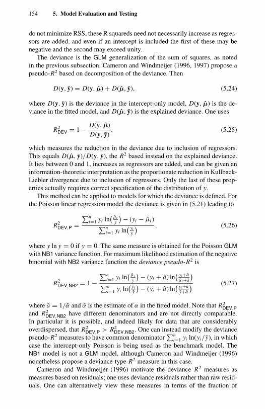
154 5. Model Evaluation and Testing

do not minimize RSS, these R squareds need not necessarily increase as regres-sors are added, and even if an intercept is included the first of these may benegative and the second may exceed unity.

The deviance is the GLM generalization of the sum of squares, as notedin the previous subsection. Cameron and Windmeijer (1996, 1997) propose apseudo-R2 based on decomposition of the deviance. Then

D(y, y) = D(y, µ) + D(µ, y), (5.24)

where D(y, y) is the deviance in the intercept-only model, D(y, µ) is the de-viance in the fitted model, and D(µ, y) is the explained deviance. One uses

R2DEV = 1 − D(y, µ)

D(y, y), (5.25)

which measures the reduction in the deviance due to inclusion of regressors.This equals D(µ, y)/D(y, y), the R2 based instead on the explained deviance.It lies between 0 and 1, increases as regressors are added, and can be given aninformation-theoretic interpretation as the proportionate reduction in Kullback-Liebler divergence due to inclusion of regressors. Only the last of these prop-erties actually requires correct specification of the distribution of y.

This method can be applied to models for which the deviance is defined. Forthe Poisson linear regression model the deviance is given in (5.21) leading to

R2DEV,P =

∑ni=1 yi ln

(µi

y

)− (yi − µi )∑ni=1 yi ln

( yi

y

) , (5.26)

where y ln y = 0 if y = 0. The same measure is obtained for the Poisson GLMwith NB1 variance function. For maximum likelihood estimation of the negativebinomial with NB2 variance function the deviance pseudo-R2 is

R2DEV,NB2 = 1 −

∑ni=1 yi ln

(µi

y

)− (yi + a) ln( yi +a

µi +a

)∑ni=1 yi ln

( yi

y

)− (yi + a) ln( yi +a

y+a

) (5.27)

where a = 1/α and α is the estimate of α in the fitted model. Note that R2DEV,P

and R2DEV,NB2 have different denominators and are not directly comparable.

In particular it is possible, and indeed likely for data that are considerablyoverdispersed, that R2

DEV,P > R2DEV,NB2. One can instead modify the deviance

pseudo-R2 measures to have common denominator∑n

i=1 yi ln(yi/y), in whichcase the intercept-only Poisson is being used as the benchmark model. TheNB1 model is not a GLM model, although Cameron and Windmeijer (1996)nonetheless propose a deviance-type R2 measure in this case.

Cameron and Windmeijer (1996) motivate the deviance R2 measures asmeasures based on residuals; one uses deviance residuals rather than raw resid-uals. One can alternatively view these measures in terms of the fraction of

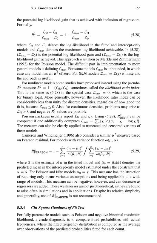
5.3. Goodness of Fit 155

the potential log-likelihood gain that is achieved with inclusion of regressors.Formally,

R2 = Lfit − L0

Lmax − L0= 1 − Lmax − Lfit

Lmax − L0, (5.28)

where Lfit and L0 denote the log-likelihood in the fitted and intercept-onlymodels and Lmax denotes the maximum log-likelihood achievable. In (5.28),(Lmax − L0) is the potential log-likelihood gain and (Lmax − Lfit) is the log-likelihood gain achieved. This approach was taken by Merkle and Zimmermann(1992) for the Poisson model. The difficult part in implementation to moregeneral models is defining Lmax. For some models Lmax is unbounded, in whichcase any model has an R2 of zero. For GLM models Lmax = L(y) is finite andthe approach is useful.

For nonlinear models some studies have proposed instead using the pseudo-R2 measure R2 = 1 − (Lfit/L0), sometimes called the likelihood ratio index.This is the same as (5.28) in the special case Lmax = 0, which is the casefor binary logit. More generally, however, the likelihood ratio index can beconsiderably less than unity for discrete densities, regardless of how good thefit is, because Lmax ≤ 0. Also, for continuous densities, problems may arise asLfit > 0 and negative R2 values are possible.

Poisson packages usually report Lfit and L0. Using (5.28), R2DEV,P can be

computed if one additionally computes Lmax = ∑i yi log yi − yi − log yi !.The measure can also be clearly applied to truncated and censored variants ofthese models.

Cameron and Windmeijer (1996) also consider a similar R2 measure basedon Pearson residual. For models with variance function ω(µ, α)

R2PEARSON = 1 −

n∑i=1

(yi − µi )2

ω(µi , α)

/ n∑i=1

(yi − µ0)2

ω(µ0, α), (5.29)

where α is the estimate of α in the fitted model and µ0 = µ0(α) denotes thepredicted mean in the intercept-only model estimated under the constraint thatα = α. For Poisson and NB2 models µ0 = y. This measure has the attractionof requiring only mean–variance assumptions and being applicable to a widerange of models. This measure can be negative, however, and can decrease asregressors are added. These weaknesses are not just theoretical, as they are foundto arise often in simulations and in applications. Despite its relative simplicityand generality, use of R2

PEARSON is not recommended.

5.3.4 Chi-Square Goodness of Fit Test

For fully parametric models such as Poisson and negative binomial maximumlikelihood, a crude diagnostic is to compare fitted probabilities with actualfrequencies, where the fitted frequency distribution is computed as the averageover observations of the predicted probabilities fitted for each count.

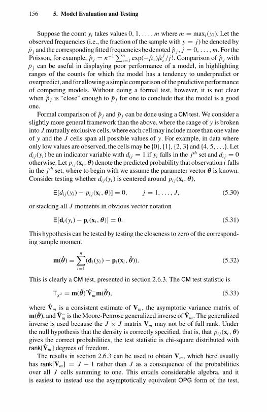
156 5. Model Evaluation and Testing

Suppose the count yi takes values 0, 1, . . . , m where m = maxi (yi ). Let theobserved frequencies (i.e., the fraction of the sample with y = j) be denoted byp j and the corresponding fitted frequencies be denoted p j , j = 0, . . . , m. For thePoisson, for example, p j = n−1∑n

i=1 exp(−µi )µji /j!. Comparison of p j with

p j can be useful in displaying poor performance of a model, in highlightingranges of the counts for which the model has a tendency to underpredict oroverpredict, and for allowing a simple comparison of the predictive performanceof competing models. Without doing a formal test, however, it is not clearwhen p j is “close” enough to p j for one to conclude that the model is a goodone.

Formal comparison of p j and p j can be done using a CM test. We consider aslightly more general framework than the above, where the range of y is brokeninto J mutually exclusive cells, where each cell may include more than one valueof y and the J cells span all possible values of y. For example, in data whereonly low values are observed, the cells may be 0, 1, 2, 3 and 4, 5, . . .. Letdi j (yi ) be an indicator variable with di j = 1 if yi falls in the j th set and di j = 0otherwise. Let pi j (xi ,θ) denote the predicted probability that observation i fallsin the j th set, where to begin with we assume the parameter vector θ is known.Consider testing whether di j (yi ) is centered around pi j (xi ,θ),

E[di j (yi ) − pi j (xi ,θ)] = 0, j = 1, . . . , J, (5.30)

or stacking all J moments in obvious vector notation

E[di (yi ) − pi (xi ,θ)] = 0. (5.31)

This hypothesis can be tested by testing the closeness to zero of the correspond-ing sample moment

m(θ) =n∑

i=1

(di (yi ) − pi (xi , θ)). (5.32)

This is clearly a CM test, presented in section 2.6.3. The CM test statistic is

Tχ2 = m(θ)′V−mm(θ), (5.33)

where Vm is a consistent estimate of Vm , the asymptotic variance matrix ofm(θ), and V−

m is the Moore-Penrose generalized inverse of Vm . The generalizedinverse is used because the J × J matrix Vm may not be of full rank. Underthe null hypothesis that the density is correctly specified, that is, that pi j (xi ,θ)gives the correct probabilities, the test statistic is chi-square distributed withrank[Vm] degrees of freedom.

The results in section 2.6.3 can be used to obtain Vm , which here usuallyhas rank[Vm] = J − 1 rather than J as a consequence of the probabilitiesover all J cells summing to one. This entails considerable algebra, and itis easiest to instead use the asymptotically equivalent OPG form of the test,

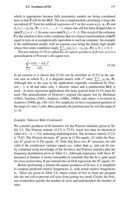
5.3. Goodness of Fit 157

which is appropriate because fully parametric models are being consideredhere so that θ will be the MLE. The test is implemented calculating n times theuncentered R2 from the artificial regression of 1 on the scores si (yi , xi , θ) anddi j (yi ) − pi j (xi , θ), j = 1, . . . , J − 1, where one cell has been dropped due torank[Vm] = J −1. In some cases rank[Vm] < J −1. This occurs if the estimatorθ is the solution to first-order conditions that set a linear transformation of m(θ)equal to zero or is asymptotically equivalent to such an estimator. An exampleis the multinomial model, with an extreme case being the binary logit modelwhose first-order conditions imply

∑ni=1(di j (yi ) − pi j (xi , θ)) = 0, j = 0, 1.

The test statistic (5.33) is called the chi-square goodness-of-fit test, as it is ageneralization of Pearson’s chi-square test,

J∑j=1

(n p j − n p j )2

n p j. (5.34)

In an exercise it is shown that (5.34) can be rewritten as (5.33) in the spe-cial case in which Vm is a diagonal matrix with i th entry

∑ni=1 pi j (xi ,θ).

Although this is the case in the application originally considered by Pear-son – yi is iid and takes only J discrete values and a multinomial MLE isused – in most regression applications the more general form (5.33) must beused. The generalization of Pearson’s original chi-square test by Heckman(1984), Tauchen (1985), Andrews (1988a, 1988b), and others is reviewed inAndrews (1988b, pp. 140–141). For simplicity we have considered partition ofthe range of y into J cells. More generally the partition may be over the range of(y, x).

Example: Takeover Bids (Continued)

We consider goodness-of-fit measures for the Poisson estimates given in Ta-ble 5.3. The Pearson statistic (5.17) is 72.52, much less than its theoreticalvalue of n − k = 116, indicating underdispersion. The deviance statistic (5.21)is 75.87. The Poisson deviance R2 given in (5.26) equals .25 while the Pear-son R2 given in (5.29) equals .35. Note that these two R2 measures are stillvalid if the conditional variance equals αµi rather than µi and can be eas-ily computed using knowledge of the deviance and Pearson statistics plus thefrequency distribution given in Table 5.1. Although experience with these R2

measures is limited, it seems reasonable to conclude that the fit is quite goodfor cross-section data. If one instead runs an OLS regression, the R2 equals .24.

Before performing a formal chi-square goodness-of-fit test, it is insightfulto compare predicted relative frequencies p j with actual relative frequenciesp j . These are given in Table 5.6, where counts of five or more are groupedinto the one cell to prevent cell sizes from getting too small. Clearly the Pois-son overpredicts greatly the number of zeros and underpredicts the number ofones.

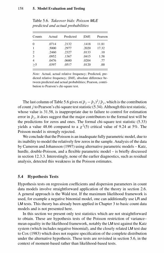
158 5. Model Evaluation and Testing

Table 5.6. Takeover bids: Poisson MLEpredicted and actual probabilities

Counts Actual Predicted |Diff| Pearson

0 .0714 .2132 .1418 11.811 .5000 .2977 .2020 17.322 .2460 .2327 .0133 .103 .0952 .1367 .0415 1.584 .0476 .0680 .0204 .77≥5 .0397 .0517 .0120 .00

Note: Actual, actual relative frequency; Predicted, pre-dicted relative frequency; |Diff|, absolute difference be-tween predicted and actual probabilities; Pearson, contri-bution to Pearson’s chi-square test.

The last column of Table 5.6 gives n( p j − p j )2/ p j , which is the contributionof count j to Pearson’s chi-square test statistic (5.34). Although this test statistic,whose value is 31.58, is inappropriate due to failure to control for estimationerror in p j , it does suggest that the major contributors to the formal test will bethe predictions for zeros and ones. The formal chi-square test statistic (5.33)yields a value 48.66 compared to a χ2(5) critical value of 9.24 at 5%. ThePoisson model is strongly rejected.

We conclude that the Poisson is an inadequate fully parametric model, due toits inability to model the relatively few zeros in the sample. Analysis of the databy Cameron and Johansson (1997) using alternative parametric models – Katz,hurdle, double-Poisson, and a flexible parametric model – is briefly discussedin section 12.3.3. Interestingly, none of the earlier diagnostics, such as residualanalysis, detected this weakness in the Poisson estimates.

5.4 Hypothesis Tests

Hypothesis tests on regression coefficients and dispersion parameters in countdata models involve straightforward application of the theory in section 2.6.A general approach is the Wald test. If the maximum likelihood framework isused, for example a negative binomial model, one can additionally use LR andLM tests. This theory has already been applied in Chapter 3 to basic count datamodels and is not presented here.

In this section we present only test statistics which are not straightforwardto obtain. These are hypothesis tests of the Poisson restriction of variance–mean equality in the likelihood framework, notably the LM test against the Katzsystem (which includes negative binomial), and the closely related LM test dueto Cox (1983) which does not require specification of the complete distributionunder the alternative hypothesis. These tests are revisited in section 5.6, in thecontext of moment-based rather than likelihood-based tests.

5.4. Hypothesis Tests 159

5.4.1 LM Test for Overdispersion against Katz System

Tests for overdispersion are tests of the variance–mean equality imposed by thePoisson against the alternative that the variance exceeds the mean. These areimplemented by tests of the Poisson with mean µi and variance µi , against thenegative binomial with mean

E[yi | xi ] = µi = µ(xi ,β) (5.35)

and variance

V[yi | xi ] = µi + αg(µi ), (5.36)

for specified function g(µi ). Usually g(µi ) = µi or g(µi ) = µ2i . The null hy-

pothesis is

H0 : α = 0. (5.37)

Such tests are easily implemented as LR, Wald, or LM tests of H0 againstHa : α > 0. These tests are presented in Chapter 3. As noted there, the usualcritical values of the LR and Wald cannot be used, and adjustment needs to bemade because the null hypothesis α = 0 lies on the boundary of the parameterspace for the negative binomial, which does not permit underdispersion.

Tests for underdispersion, or variance less than the mean, can be constructedin a similar manner. One needs a distribution that permits underdispersion andnests the Poisson. The Katz system, defined in Chapter 4, has this property. Foroverdispersed data it equals the commonly used negative binomial. For under-dispersed data, however, the Katz system model is not offered as a standardmodel in count-data packages. The LM test, which requires estimation onlyunder the null hypothesis of Poisson, is particularly attractive for the underdis-persed case.

Derivation of the LM test of Poisson against the Katz system, due to Lee(1986), who considered g(µi ) = µi and g(µi ) = µ2

i , is not straightforward.In section 5.8 it is shown that for the Katz system density with mean µi andvariance µi + αg(µi )

∂L∂β

∣∣∣∣α=0

=n∑

i=1

µ−1i (y − µi )

∂µi

∂β

∂L∂α

∣∣∣∣α=0

=n∑

i=1

1

2µ−2

i g(µi )(yi − µi )2 − yi .

(5.38)

The LM test is based on these derivatives evaluated at the restricted MLE,which is θ = (β

′α)′ = (β

′0)′ where β is the Poisson MLE. But the first

summation in (5.38) equals the derivative with respect to β of the Poisson log-likelihood with general conditional mean µi (β), so ∂L/∂β|β=β,α=0 = 0 andhence

∂L∂θ

∣∣∣∣β=β,α=0

=[

0∑ni=1 µ−2

i g(µi ) 12 (yi − µi )2 − yi

]. (5.39)

160 5. Model Evaluation and Testing

To construct the LM test stated earlier in section 2.6.1, we additionally needa consistent estimate of the variance matrix, which by the information matrixequality is the limit of T −1E[(∂L/∂θ|α=0)(∂L/∂θ′|α=0)]. Now under the nullhypothesis that y ∼ P[µ],

E[(y − µ)2] = µ

E[(y − µ)2 − y(y − µ)] = 0 (5.40)

E[(y − µ)2 − y2] = 2µ2.

This implies

E

[∂2L

∂θ∂θ′

∣∣∣∣α=0

]=[∑n

i=1 µ−1i

∂µi

∂β∂µi

∂β′ 00

∑ni=1

12µ−2

i g2(µi )

].

(5.41)

Given (5.39) and (5.41) the LM test statistic in section 2.6.1 is constructed. Thiswill be a (k + 1) × (k + 1) matrix with zeros everywhere except for the lastdiagonal entry. Taking the square root of this scalar yields

TLM =[

n∑i=1

1

2µ−2

i g2(µi )

]−1/2 n∑i=1

1

2µ−2

i g(µi )(yi − µi )2 − yi .

(5.42)

Because the negative binomial is the special case α > 0 of the Katz sys-tem, this statistic is the LM test for Poisson against both negative binomialoverdispersion and Katz system underdispersion. At significance level .05, forexample, the null hypothesis of equidispersion is rejected against the alternativehypothesis of overdispersion if TLM > z.05, underdispersion if TLM < −z.05 andover- or underdispersion if |TLM| > z.025.

Clearly one can obtain different LM test statistics by nesting the Poisson inother distributions. In particular Gurmu and Trivedi (1993) nest the Poissonin the double-Poisson, a special case of nesting the LEF in the extended LEF,which they more generally consider, and obtain a test statistic for overdispersionthat is a function of the deviance statistic.

The LM test for Poisson against negative binomial has been extended to pos-itive Poisson models by Gurmu (1991) and to left- and right-truncated Poissonmodels by Gurmu and Trivedi (1992). These extensions involve a number ofcomplications, including non–block-diagonality of the information matrix sothat the off-diagonal elements in the generalization of (5.41) are nonzero.

5.4.2 Auxiliary Regressions for LM Test

As is usual for test statistics, there are many asymptotically equivalent versionsunder H0 of the overdispersion test statistic TLM given in (5.42). Several of these

5.4. Hypothesis Tests 161

can be easily calculated from many different auxiliary OLS regressions. LikeTLM they are distributed as N[0, 1], or χ2(1) on squaring, under H0.

The auxiliary OPG regression for the LM test given in section 2.6.1 uses theuncentered explained sums of squares from OLS regression of 1 on 1

2 µ−2i g(µi )

(yi − µi )2 − yi and µ−1i (yi − µi )∂µi/∂β|β. The square root of this is asymp-

totically equivalent to TLM.An asymptotically equivalent variant of this auxiliary regression is to use the

uncentered explained sums of squares from OLS regression of 1 on 12 µ−2

i g(µi )(yi − µi )2 − yi alone. This simplification is possible, as 1

2 µ−2i g(µi )(yi −

µi )2 − yi and µ−1i (yi − µi )∂µi/∂β|β are asymptotically uncorrelated because

for the Poisson E[(yi − µi )2 − yi (yi − µi )] = 0 by (5.40), and because∑ni=1 µ−1

i (yi − µi )∂µi/∂β|β = 0 by the first-order conditions for the H0

Poisson MLE. The square root of the explained sum of squares is

T∗LM =

[n∑

i=1

(1

2

)2

µ−4i g2(µi )(yi − µi )

2 − yi 2

]−1/2

(5.43)

×n∑

i=1

1

2µ−2

i g(µi )(yi − µi )2 − yi ,

using the result that the square root of the uncentered explained sum of squaresfrom regression of y∗

i on the scalar xi is (∑

i x2i )−1/2∑

i xi y∗i . This test is

asymptotically equivalent to TLM, as for the Poisson

E

[1

2µ−2

i (yi − µi )2 − yi 2

]= 1, (5.44)

by the last equation in (5.40).In the special case g(µi ) = µl

i , Cameron and Trivedi (1986) proposed usingan alternative variant of TLM. For general g(µi ) this variant becomes

T∗∗LM=[

1

n

n∑i=1

1

2µ−2

i (y − µi )2 − yi 2

]−1/2[ n∑i=1

1

2µ−2

i g2(µi )

]−1/2

×n∑

i=1

1

2µ−2

i g(µi )(yi − µi )2 − yi . (5.45)

This is asymptotically equivalent to TLM because the first term in parentheseshas plim unity by (5.44). This can be computed as the square root of n times theuncentered explained sum of squares from the OLS regression of 1

2 µ−1i (yi −

µi )2 − yi against 12 µ−1

i g(µi ).In general the t test from the regression y∗

i = αxi + ui , where xi is a scalar,can be shown to equal (1/s)(

∑i x2

i )−1/2∑i xi y∗

i , where s is the standard errorof this regression. For the regression

(√

2µi )−1(yi − µi )

2 − yi = (√

2µi )−1g(µi ) α + vi , (5.46)

162 5. Model Evaluation and Testing

it follows that the t statistic for α = 0 is

T∗∗∗LM =

[s2

n∑i=1

1

2µ−2

i g2(µi )

]−1/2 n∑i=1

1

2µ−2

i g(µi )(yi − µi )2 − yi ,

(5.47)

where

s2 = 1

n − 1

n∑i=1

(√

2µi )−2(yi − µi )

2 − yi − g(µi ) α2. (5.48)

This test is asymptotically equivalent to TLM, because plim s2 = 1 under H0

on setting α = 0 and using the moment condition (5.44). This is the regressiongiven in section 3.4, on elimination of 1

2 from both sides of the regression andletting g(µi ) = µ2

i for tests against NB2 and g(µi ) = µi for tests against NB1.In principle the LM test statistic can be computed using any of these many

auxiliary regressions, as they are all asymptotically equivalent under H0. Inpractice the computed values can differ significantly. This is made clear bynoting that asymptotic equivalence is established using assumptions, such asE[(yi − µi )2 − yi 2] = 2µi , which hold only under H0.

The regression (5.46) has a physical interpretation, in addition to being acomputational device. It can be viewed as a WLS regression based on testingwhether α = 0 in the population moment condition

E[(yi − µi )2 − yi ] = αg(µi ). (5.49)

This moment condition is implied by the alternative hypothesis given by (5.35)and (5.36). Tests based on (5.49) of overdispersion or underdispersion, undermuch weaker stochastic assumptions than Poisson against the Katz system,were proposed by Cameron and Trivedi (1985, 1990a). Their testing approachis presented in section 5.6.

5.4.3 LM Test against Local Alternatives

Cox (1983) proposed a quite general method to construct the LM test statisticwithout completely specifying the density under the alternative hypothesis. Thegeneral result is presented before specialization to overdispersion tests.

Let y have density f (y | λ), where the scalar parameter λ is itself a randomvariable, distributed with density p(λ | µ, τ ) where µ and τ denote the mean andvariance of λ. This mixture distribution approach has already been presentedin Chapter 4. For example, if y is Poisson-distributed with parameter λ whereλ is gamma-distributed, then y is negative binomial distributed, conditional onthe gamma distribution parameters.

Interest lies in the distribution of y given µ and τ

h(y | µ, τ ) =∫

f (y | λ)p(λ | µ, τ ) dλ. (5.50)

5.5. Inference with Finite Sample Corrections 163

A second-order Taylor series expansion of f (y | λ) about λ = µ yields

h(y | µ, τ ) =∫

f (y | µ) + f ′(y | µ)(λ − µ)

+ 1

2f ′′(y | µ)(λ − µ)2 + Rp(λ | µ, τ ) dλ (5.51)

where f ′(·) and f ′′(·) denote the first and second derivatives, respectively, andR is a remainder term. Cox (1983) considered only small departures of λ fromits mean of µ, specifically V[λ] = τ = δ/

√n, where δ is finite nonzero. After

considerable algebra, given in section 5.8, this can be reexpressed as

h(y | µ, τ ) = f (y | µ) exp

[1

2τ

∂2 ln f (y | µ)

∂µ2

+(

∂ ln f (y | µ)

∂µ

)2]+ O(n−1). (5.52)

Cox (1983) considered LM (or score) tests against this approximation to thealternative hypothesis density, which from 5.52 reduces to the null hypothesisdensity f (y | µ) if τ = 0.

For application to the Poisson we suppose V[λ] = τ = δg(µ)/√

n, whichimplies V[y] = µ + δg(µ)/

√n. Then in (5.36) we are considering local al-

ternatives α = δ/√

n. The log-likelihood under local alternatives is L =∑ni=1 ln h(yi | µi , τ ) and

∂L∂α

∣∣∣∣α=0

=n∑

i=1

1

2g(µi )

∂2 ln f (yi | µi )

∂µ2i

+(

∂ ln f (yi | µi )

∂µi

)2.

(5.53)

If f (yi | µi ) is the Poisson density this yields

∂L∂α

∣∣∣∣α=0

=n∑

i=1

1

2g(µi )µ

−2i (yi − µi )

2 − yi , (5.54)

which is exactly the same as the second term in (5.38). The first term, ∂L/∂β|α=0

is also the same as in (5.38), and the LM test statistic is TLM, given in (5.42).The approach of Cox (1983) demonstrates that TLM in (5.42) is valid for

testing Poisson against all local alternatives satisfying (5.35) and (5.36), not justthe Katz system. The general form (5.52) for the density under local alternativesis clearly related to the information matrix equality. In section 5.6.5 we makethe connection between the Cox test and the information matrix test.

5.5 Inference with Finite Sample Corrections

A brief discussion of small-sample performance of hypothesis tests in the Pois-son and negative binomial models is given by Lawless (1987b). He concluded

164 5. Model Evaluation and Testing

that the LR test was preferable for tests on regression coefficients, althoughnone of the methods worked badly in small samples. There was, however, con-siderable small-sample bias in testing dispersion parameters.

The standard general procedure to handle small-sample bias in statisticalinference is the bootstrap, proposed by Efron (1979) and presented in the nextsubsection. This method has to date not been widely applied to count models.One potential complication is that the bootstrap requires resampling from aniid distribution, but the errors in cross-section count data models are typicallynot identically distributed.

The main application of small-sample corrections for count data analysis hasbeen a method quite different from the bootstrap, one proposed by Dean andLawless (1989a) for LM tests of overdispersion. This method has been appliedin several studies, which find in simulations that the improved size performanceis small except if sample sizes are small, say less than 30 observations.

5.5.1 Bootstrap

The bootstrap, introduced by Efron (1979), is a method to obtain the distributionof a statistic by resampling from the original data set. An introductory treatmentis given by Efron and Tibsharani (1993). An excellent treatment with emphasison common regression applications is given by Horowitz (1997). Here we focuson application to cross-section count data regression models, particularly thePoisson PMLE, using the bootstrap pairs procedure under the assumption that(yi , xi ) is iid.

Reasons for performing a bootstrap in estimation and statistical inferenceinclude weaker stochastic assumptions, simpler computation, and potentiallybetter small-sample performance. The first two reasons are often compellingreasons for using the bootstrap in applied work even if small-sample perfor-mance gains are not achieved. An example of using the bootstrap under weakerstochastic assumptions has been given in section 3.2.6, where the standard errorof the Poisson PMLE was obtained under the assumption that (yi , xi ) is iid andE[yi | xi ] = exp(x′

iβ). Here V[yi | xi ] is not specified, and the distributional as-sumptions are similar to those made in obtaining the robust sandwich standarderrors. Examples of simpler computation include obtaining the distribution ofr(θ), in applications in which r(·) is a complicated function of θ, by bootstraprather than the delta method given in section 2.6.2; and obtaining the distri-bution of a sequential two-step estimator by bootstrap, rather than the methoddiscussed in section 2.5.3 and detailed in Newey (1984). Despite these otheradvantages, the statistical literature has focused on small-sample performanceof the bootstrap.

The bootstrap can be applied to estimation of moments of the distributionof a statistic, testing hypotheses, and construction of confidence intervals.

We begin with use of the bootstrap to estimate standard errors. Let θ j denotethe estimator of the j th component of the parameter vector θ. The bootstrapprocedure is as follows:

5.5. Inference with Finite Sample Corrections 165

1. Form a new pseudosample of size n, (y∗l , x∗

l ), l = 1, . . . , n, by sam-pling with replacement from the original sample (yi , xi ), i = 1, . . . , n.

2. Obtain the estimator, say θ1 with j th component θ j,1, using the pseu-dosample data.

3. Repeat steps 1 and 2 B times giving B estimates θ j,1, . . . , θ j,B .4. Estimate the standard deviation of θ j using the usual formula for the

sample standard deviation of θ j,1, . . . , θ j,B , or

seBoot[θ j ] =√√√√ 1

B − 1

B∑b=1

(θ j,b − θ j )2 (5.55)

where θ j is the usual sample mean θ j = (1/B)∑B

b=1 θ j,b. The esti-mated standard error is the square root of VBoot[θP, j ].

The bootstrap is very easy to implement in this example, given a resamplingalgorithm and a way to save parameter estimates from the B simulations. Theonly drawback is that if estimating the model once takes a long time, estimatingit B times may be too computationally burdensome. Efron and Tibshirani (1993,p. 52) state that B = 200 is generally sufficient for standard error estimation.The method is easily adapted to statistics other than an estimator – replace θby the statistic of interest, and to estimates of moments other than the samplestandard deviation.

The bootstrap can additionally provide improved estimation of the distribu-tion of a statistic in small samples, in the sense that as n → ∞ the bootstrapestimator converges faster than the usual first-order asymptotic theory. Thesegains occur because in some cases it is possible to construct the bootstrap asa numerical method to implement an Edgeworth expansion, which is a morerefined asymptotic theory than the usual first-order theory. A key requirementfor improved small-sample performance of the bootstrap is that the statisticbeing considered is asymptotically pivotal, which means that the asymptoticdistribution of the statistic does not depend on unknown parameters.

We present a version of the bootstrap for hypothesis tests that yields improvedsmall-sample performance. Consider testing the hypothesis H0 : θ j = θ j0

against H0 : θ j = θ j0, where estimation is by the Poisson PMLE. The t statisticused is t j = (θ j − θ j0)/s j , where s j is the robust sandwich standard errorestimate for θ j which assumes that (yi , xi ) is iid. On the basis of first-orderasymptotic theory, we would reject H0 at level α if |t j | > zα/2.

The bootstrap procedure to test H0 is as follows:

1. Form a new pseudosample of size n, (y∗l , x∗

l ), l = 1, . . . , n, by sam-pling with replacement from the original sample (yi , xi ), i = 1, . . . , n.

2. Obtain the estimator θ j,1, the standard error s j,1, and the t statistict j,1 = (θ j,1 − θ j0)/s j,1 for the pseudosample data.

3. Repeat steps 1 and 2 B times, yielding t j,1, . . . , t j,B .4. Order these B t statistics and calculate t j,[α/2] and t j,[1−α/2], the lower

and upper α/2 percentiles of t j,1, . . . , t j,B .

166 5. Model Evaluation and Testing

5. Reject H0 at level α if t j , the t statistic from the original sample, fallsoutside the interval (t j,[α/2], t j,[1−α/2]).

For confidence intervals the same bootstrap procedure is used, except thatat step 2 one forms t∗

j,1 = (θ j,1 − θ j )/s j,1, centering around the estimate of θ j

from the original example, and at the last stage one constructs the 100(1 −α)%confidence interval (θ j − t∗

j,[α/2]s j , θ j + t∗j,[1−α/2]s j ).

This bootstrap procedure leads to an improved small-sample performancein the following sense. Let α be the nominal size for a test procedure. Usualasymptotic theory produces t tests with actual size α + O(n−1/2), whereasthis bootstrap produces t tests with actual size α + O(n−1). This refinementis possible because it is the t statistic, whose asymptotic distribution does notdepend on unknown parameters, that is bootstrapped. For both hypothesis testsand confidence intervals the number of iterations should be larger than forstandard error estimation, say B = 1000.

An alternative bootstrap method is the percentile method. This calculatesθ j,[α/2] and θ j,[1−α/2], the lower and upper α/2 percentiles of θ j,1, . . . , θ j,B .Then one rejects H0 : θ j = θ j0 against Ha : θ j = θ j0 if θ j0 does not lie in(θ j,[α/2], θ j,[1−α/2]), and one uses (θ j,[α/2], θ j,[1−α/2]) as the 100(1 − α)% confi-dence interval. This alternative procedure is asymptotically valid but is no betterthan using the usual asymptotic theory because it is based on the distributionof θ j , which unlike t j depends on unknown parameters. Similarly, using theusual hypothesis tests and confidence intervals, with the one change that s j isreplaced by a bootstrap estimate, is asymptotically valid but no better than theusual first-order asymptotic methods.

These alternative approaches illustrate the need to bootstrap the right statis-tic to achieve small-sample performance gains. Theoretically inferior methodsmay still be very useful in actual applications, however, as they do not requirecomputation of s j using potentially complicated asymptotic results. Also, forvery large samples there may be little need for asymptotic refinements.

The bootstrap can also be used for bias correction. Consider estimation ofθ j , the j th component of θ. Let θ j denote the usual estimator of θ j using theoriginal sample, and let θ j denote the average over B bootstrap replications ofthe bootstrap estimates. The estimator θ j is a bootstrap measure of E[θ j ], so thebootstrap estimate of bias is (θ j − θ j ). Before giving a general formula, considera specific example of bias correction in which θ j = 4 and θ j = 5. Then θ j isupward-biased with bias of 1 because the bootstrap estimate of E[θ j ] is 5. Tocorrect for this upwards bias in the estimator θ j we subtract the bias from thesample estimate θ j , giving a bias-corrected estimate of 3. More generally, thebias-corrected estimate of θ j is θ j − (θ j − θ j ) = 2θ j − θ j . Note that the bias-corrected estimate of θ j is not θ j . Efron and Tibsharani (1993, p. 138) provideseveral other caveats on using the bootstrap for bias correction.

A key requirement for validity of the bootstrap is that resampling be doneon a quantity that is iid. The bootstrap pairs procedure ensures this, resamplingjointly the pairs (yi , xi ), which are assumed to be iid. In the linear model withhomoskedastic errors an alternative and more commonly used procedure is

5.5. Inference with Finite Sample Corrections 167

to bootstrap or resample the residuals. Efron and Tibshirani (1993, p. 113)discuss bootstrapping pairs, rather than residuals, for the linear model with iiderrors where both approaches are possible. For count data, bootstrapping theresiduals is not valid as the errors are heteroskedastic, for example, and thereforenot iid.

Horowitz (1997) gives a detailed example of bootstrap hypothesis tests for thelinear model with heteroskedasticity. In addition to bootstrap pairs, he uses thewild bootstrap of Liu (1988); see also Mammen, 1993), which imposes onthe bootstrap the restriction that the conditional mean of the error is zero. Thewild bootstrap performs considerably better than bootstrapping pairs. Thesemethods can be adapted to the Poisson PMLE. Presumably further gains can beobtained by imposing any additional moment assumptions that might be made,such as the GLM assumption that the variance is a multiple of the mean. Forfully parametric models such as the hurdle model one can perform hypothesistests using a parametric bootstrap.

For time series data, dependence is a potential problem. In the linear model itis accounted for by assuming an autoregressive moving average error structureand resampling the underlying white noise error, or by using the moving-blocksbootstrap in which blocks are independent but the correlation structure withinblocks is preserved. These time series methods are in their infancy.

5.5.2 Other Corrections

Small-sample corrections to testing in count data models have rarely been done,although this should change rapidly as the bootstrap becomes increasingly used.To date the leading example of small-sample correction in count models hasbeen to LM tests for overdispersion, using an approach due to Dean and Law-less (1989a), which differs from the Edgeworth expansion and bootstrap. Thismethod can be applied to any GLM, not just the Poisson.

Dean and Lawless (1989a) considered the LM test statistic for Poisson againstNB2 given in (5.42). The starting point is the result in McCullagh and Nelder(1983, appendix C) that for GLM density with mean µi and variance V[yi ], theresidual (yi − µi ) has approximate variance (1 − hii )V[yi ], where hii is the i th

diagonal entry of the hat matrix H defined in (5.12). Applying this result to thePoisson, it follows that

E[(yi − µi )2 − yi ] (1 − hi i )µi − µi −hii µi . (5.56)

This leads to small-sample bias under H0 : E[(yi − µi )2 − yi ], which can becorrected by adding hi i µi to components of the sum in the numerator of (5.42),yielding the adjusted LM test statistic

TaLM =

[n∑

i=1

1

2µ−2

i g2(µi )

]−1/2

×n∑

i=1

1

2µ−2

i g(µi )(yi − µi )2 − yi + hi i µi . (5.57)

168 5. Model Evaluation and Testing

For the Poisson with exponential mean function, hi i is the i th diagonal entry inW1/2X(X′WX)−1X′W1/2 where W = Diag[µi ] and X is the matrix of regres-sors.

Dean and Lawless (1989a) considered tests of Poisson against NB2 overdis-persion, g(µi ) = µ2

i . The method has also been applied to other GLM models.Application to overdispersion in the binomial model is relatively straightfor-ward and is presented in Dean (1992). Application to a truncated Poisson model,also a GLM, is considerably more complex and is given by Gurmu and Trivedi(1992). For data left-truncated at r , meaning only yi ≥ r is observed, theadjusted LM test for Poisson against negative binomial is

TaLM = [Iαα]−1/2

n∑i=1

1

2µ−2

i g(µi )

× (yi − µi )2 − yi + (2yi − µi − r + 1)λ(r − 1, µi )µi ,

where Iαα is the scalar subcomponent for α of the inverse of the informationmatrix −E[∂2L/∂θ∂θ′] evaluated at θ = (β

′, 0)′, see Gurmu and Trivedi (1992,

p. 350), and λ(r − 1, µ) = f (y, µ)/1 − F(y, µ) where f (·) and F(·) are theuntruncated Poisson density and cdf.

The procedure has a certain asymmetry in that a small-sample correctionis made only to the term in the numerator of the score test statistic. Conniffe(1990) additionally considered correction to the denominator term.

This method for small-sample correction of heteroskedasticity tests is muchsimpler than using the Edgeworth expansion, which from Honda (1988) issurprisingly complex even for the linear regression model under normality. Themethod cannot be adapted to tests of the regression coefficients themselves,however, as the score test in this case involves a weighted sum of (yi − µi ) andthe above method yields a zero asymptotic bias for (yi − µi ). Small-sampleadjustments are most easily done using the bootstrap, which as already notedis actually an empirical implementation of an Edgeworth expansion.

5.6 Conditional Moment Specification Tests

Likelihood-based hypothesis tests, for overdispersion, were presented in sec-tion 5.4. In this section we instead take a moment-based approach to hypothesistesting, using the CM test framework. The general approach is outlined in sec-tion 5.6.1. See also section 2.6.3 for motivation and general theory. The focus ison CM tests of correct specification of the mean and variance. Key results, andlinks to the LM tests presented earlier, are given in section 5.6.2. Generalizationof these results to general cross-section models is given in section 5.6.3. Insection 5.6.4 we present CM tests based on orthogonal polynomials in (y − µ),an alternative way to use the low-order moments of y. Two commonly used CMtests, the Hausman test and the information test, are presented in, respectively,sections 5.6.5 and 5.6.6.

5.6. Conditional Moment Specification Tests 169

One conclusion from this section is that many insights gained from the linearregression model with homoskedastic errors require substantial modificationbefore being applied to even the simple Poisson model models. This is becausethe Poisson has complications of both nonlinear conditional mean function andheteroskedasticity that is a function of that mean. A better guide is provided bya binary choice model, such as logit or probit. But even this is too limited asthe variance function cannot be misspecified in binary choice models, becauseit is always the mean times one minus the mean, whereas with count datathe variance function is not restricted to being that imposed by the Poissonregression model.

5.6.1 Introduction

Suppose a model implies the population moment condition

E[mi (yi , xi ,θ)] = 0, i = 1, . . . , n, (5.58)

where mi (·) is an r × 1 vector function. A CM test of this moment condition isbased on the closeness to zero of the corresponding sample moment condition,that is

m(θ) =n∑

i=1

mi ,

where mi = mi (yi , xi , θ). The CM test statistic in general is

n∑i=1

m′i

V

[n∑

i=1

mi

]−1 n∑i=1

mi ,

and is asymptotically chi-square distributed.Two issues arise in applying CM tests. First is choice of the function mi (·).

Here we focus on tests based on the first two moments of count data regressionmodels. Second is choosing how to implement the test. Several asymptoticallyequivalent versions are available, some of which can be computed using an aux-iliary regression. Here we focus on applications in which the moment conditionis chosen so that mi (·) satisfies

E

[∂mi (yi , xi ,θ)

∂θ′

]= 0. (5.59)

Then from section 2.6.3 the CM test statistic simplifies to

n∑i=1

m′i

[n∑

i=1

E[mi m′

i

]∣∣θ

]−1 n∑i=1

mi . (5.60)

170 5. Model Evaluation and Testing

If mi (·) is a scalar, taking the square root of (5.60) yields the test statistic

TCM =[

n∑i=1

E[m2

i

]∣∣θ

]−1/2 n∑i=1

mi , (5.61)

which is asymptotically N[0, 1] if (5.58) and (5.59) hold. An asymptoticallyequivalent version is

T∗CM =

[ n∑i=1

m2i

]−1/2 n∑i=1

mi . (5.62)

Even if (5.59) does not hold, implementation is still simple, provided θ is theMLE. Then a chi-square test statistic is the uncentered explained sum of squaresfrom regression of 1 on mi and si , where si = ∂ ln f (yi | xi ,θ)/∂θ|θ.

If possible CM tests are compared to the LM test, which is a special case of aCM test and is, of course, the most powerful test if a fully parametric approachis taken. Particular interest lies in tests of correct specification of the conditionalmean and variance.

For the Poisson regression, the LM test for exclusion of the subcomponentx2i of xi = [x′

1i , x′2i ]

′ model is a CM test of

E[mi (yi , xi ,β1)] = E[(yi − µ1i )x2i ] = 0, (5.63)

where µ1i = exp(x′1iβ1).

For overdispersion, the test of Poisson with variance µi = µ(x′iβ) against

the Katz system with variance function µi +αg(µi ) is from (5.39) a CM test of

E[mi (yi , xi ,β)] = E[(yi − µi )2 − yi µ−2

i g(µi )] = 0. (5.64)

Note that the simplifying condition (5.59) holds for mi (yi , xi ,β) in (5.64),provided (5.64) holds and E[yi − µi ] = 0. It can be shown that for the momentcondition (5.64) the test statistic (5.61) yields TLM given in (5.42), and the teststatistic (5.62) yields T∗

LM given in (5.43).CM tests can be obtained under relatively weak stochastic assumptions. Sev-

eral examples are given here, beginning with one in which a regression providesthe motivation or basis for the test rather than just providing a way to calculatea test statistic.

5.6.2 Regression-Based Tests for Overdispersion

Consider cross-section data (yi , xi ) where under the null hypothesis the firsttwo moments are those of the Poisson regression model

H0 : E[yi | xi ] = µi = µ(xi ,β), V[yi | xi ] = µi , (5.65)

while under the alternative hypothesis

Ha : E[yi | xi ] = µi = µ(xi ,β), V[yi | xi ] = µi +αg(µi ), (5.66)

5.6. Conditional Moment Specification Tests 171

where g(µi ) is a specified function such as µi or µ2i . The moments (5.66) are

those of, for example, the negative binomial models presented in section 3.3.The moment condition (5.66) implies

Ha : E[(yi − µi )2 − yi |xi ] = αg(µi ), (5.67)

while H0 imposes the constraint that α = 0. If µi is known one could perform a ttest of α = 0 based on regression of (yi −µi )2 − yi on g(µi ). Two complicationsare that µi is unknown and that the error term in this regression is in generalheteroskedastic as the conditional variance of (yi − µi )2 − yi is a function ofµi , say

ωi = ω(µi ) = V[(yi − µi )2 − yi |xi ]. (5.68)

The null hypothesis

H0 : α = 0 (5.69)

can be tested by the t test of α = 0 in the LS regression√ωi (yi − µi )

2 − yi = α√

ωi g(µi ) + ui , (5.70)

where µi = µ(x′i β), ωi = ω(µi ) and β is a consistent estimator of β under

H0. The WLS regression is used as it yields the most efficient least-squaresregression estimator of α and hence the most powerful or optimal test. In prin-ciple replacing µi by µi leads to a more complicated distribution for α. Thisis not a problem in this particular application, however, essentially because∂(yi − µi )2 − yi /∂β = −2(yi − µi )∂µi/∂β has expected value 0 so (5.59)holds.

Standard results for OLS yields the t test statistic α/√

V[α] or

TOLSCM =

[s2

n∑i=1

ω−1i g2(µi )

]−1/2 n∑i=1

ω−1i g(µi )(yi − µi )

2 − yi ,(5.71)

where

s2 = 1

n − 1

n∑i=1

ω−1i (yi − µi )

2 − yi − g(µi ) α2.

Under H0, plim s2 = 1 as α = 0, and one can equivalently use

TCM =[

n∑i=1

ω−1i g2(µi )

]−1/2 n∑i=1

ω−1i g(µi )(y − µi )

2 − yi .(5.72)

Advantages of this approach to testing, beyond simplicity of use, include

172 5. Model Evaluation and Testing

1. If the first four moments of yi under the null hypothesis are those of thePoisson, TCM equals the optimal LM test statistic for testing Poissonagainst the Katz system.

2. The test is easily adapted to situations in which assumptions on onlythe first two moments are made.

3. The test can be given a simple interpretation as a CM test based on thefirst two moments of yi .

4. The test is computed from an OLS regression that has interpretationas a model, rather than merely a computational device to compute thestatistic.

5. The approach can be generalized to other testing situations.

These points are made clear in the following discussion.First, in the fully parametric situation in which yi ∼ P[µi ], using formulae

for the first four moments of the Poisson one obtains ωi = 2µ2i . But then TOLS

CM in(5.71) equals T∗∗∗

LM , the LM test for Poisson against negative binomial presentedin (5.47), while TCM in (5.72) equals TLM given in (5.42).

Second, consider adaptation of the test statistic (5.71) in the case in whichonly the first two moments of yi are assumed. Then ωi in (5.68) is unknown.The least-squares regression (5.70) is again run, but with weighting function ωi

replaced by vi . One might choose vi = 2µ2i , although one should note that it is

no longer assumed that ωi = 2µ2i . Now the error ui has heteroskedasticity of

unknown functional form, so the t test of α = 0 uses robust sandwich standarderrors. The test statistic is

TRobustCM =

[n∑

i=1

u2i v

−1i g2(µi )

]−1/2 n∑i=1

v−1i g(µi )(yi − µi )

2 − yi ,(5.73)

where u2i = (yi − µi )2 − yi − αg(µi )2 and α is the least-squares estimator in

(5.70) with ωi replaced by vi . Under H0, TRobustCM is asymptotically N[0, 1].

In the special case in which vi = 2µ2i the test statistic (5.73) provides a

variant of the LM test statistic for overdispersion given in section 5.4 that isrobust to misspecification of the third and fourth moments of yi . This is directlyanalogous to the modification of the Breusch-Pagan LM test for heteroskedas-ticity in the regression model under normality proposed by Koenker (1982) toallow for nonconstant fourth moments of the dependent variable.

Third, consider a CM test for variance–mean equality. The null hypothesis(5.65) implies that

E[(yi − µi )2 − yi |xi ] = 0, (5.74)

which in turn implies

E[h(µi )(yi − µi )2 − yi ] = 0, (5.75)

5.6. Conditional Moment Specification Tests 173

where we let h(µi ) be a specified scalar function. The test based on closenessto zero of

∑ni=1 h(µi )(yi − µi )2 − yi is a special case of the CM chi-square

test statistic given in section 2.6.3. Because ∂(yi − µi )2 − yi /∂β = −2(yi −µi )∂µi/∂β has expected value 0 and so (5.59) holds, one can use TCM given in(5.61)

TCM =[

n∑i=1

h2(µi )ωi

]−1/2 n∑i=1

h(µi )(yi − µi )2 − yi , (5.76)

where ωi = E[(yi −µi )2 − yi 2|xi ]. TCM is asymptotically N[0, 1] under (5.74).This test specifies only a moment condition under H0. Different choices offunction h(µi ) will test in different directions away from H0, with the optimalchoice of h(µi ) depending on the particular alternative to (5.74). The regression-based approach makes it clear that if the alternative is (5.67) then the optimalchoice is h(µi ) = ω−1

i g(µi ).Fourth, consider calculation of overdispersion test statistics by an auxil-

iary regression. The usual approach is to obtain a CM or LM test statistic andthen give ways to calculate the statistic or an asymptotically equivalent vari-ant of the statistic by an auxiliary regression. This regression has no physicalinterpretation, being merely a computational device. Such tests are best calledregression-implemented tests, although they are often called regression-basedbecause their computation is based on a regression. By comparison the overdis-persion test statistic given in this subsection is regression-based in the strongersense that there is a regression motivation for the test statistic.

The final point, that this regression-based or regression-motivated test ap-proach generalizes to other testing situations, is outlined in the next subsection.

Regression-based tests for overdispersion were proposed by Cameron andTrivedi (1985, 1990a). In addition to the regression (5.70) they also consideredthe t test of α = 0 in the least-squares regression√

ωi (yi − µi )2 − µi = α

√ωi g(µi ) + ui . (5.77)

This replaces yi by µi in the left-hand side, the rationale being that the momentcondition (5.66) implies not only (5.67) but also

Ha : E[(yi − µi )2 − µi | xi ] = αg(µi ). (5.78)

The test based on the regression (5.77) is more difficult to implement becausereplacing µi by µi makes a difference in this regression, because ∂(yi −µi )2 −µi /∂β = −2(yi − µi ) + 1∂µi/∂β has nonzero expected value. Cameronand Trivedi (1985) show that the analog of (5.72) is

TCM,2 =[

n∑i=1

n∑j=1

wi j g(µi )g(µ j )

]−1/2

×n∑

i=1

n∑j=1

wi j g(µi )(y j − µ j )2 − µ j , (5.79)

174 5. Model Evaluation and Testing

where wi j is the ijth entry in W = [D − ∆(∆′D−1µ ∆)−1∆′]−1, D and Dµ are

n × n diagonal matrices with i th entries (2µ2i + µi ) and µi , respectively, and

∆ is an n × k matrix with i th row ∂µi/∂β′.

The test TCM,2 is a different test from TCM in (5.72), with different powerproperties. In particular TCM,2 is the LM test, and hence the most powerful test,for testing N[µi , µi ] against N[µi , µi +αg(µi )]. It has already been shown thatTCM is the LM test for P[µi ] against NB2. In addition to greater power in thestandard setup for overdispersion tests, TCM has the advantage of being easierto implement.

5.6.3 Regression-Based CM Tests

Suppose that a specified model imposes the conditional moment restriction

E[r (yi , xi ,θ) | xi ] = 0, (5.80)

where for simplicity r (·) is a scalar function. Suppose we wish to test this restric-tion against the specific alternative conditional expected value for r (yi , xi ,θ)

E[r (yi , xi ,θ) | xi ] = g(xi ,θ)′α, (5.81)

where g(·) and α are p × 1 vectors.The moment condition (5.80) can be tested against (5.81) by test of α = 0

in the regression

r (yi , xi ,θ) = g(xi ,θ)′α + εi . (5.82)

The most powerful test of α = 0 is based on the efficient GLS estimator, whichfor data independent over i is the WLS estimator

α =[

n∑i=1

1

σ 2(xi ,θ)g(xi ,θ)g(xi ,θ)′

]−1

×n∑

i=1

1

σ 2(xi ,θ)g(xi ,θ)r (yi , xi ,θ), (5.83)

where

σ 2(xi ,θ) = E0[r (yi , xi ,θ)2 | xi ] (5.84)

is the conditional variance of r (yi , xi ,θ) under the null hypothesis model.Tests based on α are equivalent to tests based on any full rank transforma-

tion of α. Most simply multiply by∑n

i=1 σ−2(xi ,θ)g(xi ,θ)r (yi , xi ,θ). This isequivalent to a CM test of the unconditional moment condition

E[m(yi , xi ,θ)] = E

[1

σ 2(xi ,θ)g(xi ,θ)r (yi , xi ,θ)

]= 0. (5.85)

Note that the unconditional moment (5.85) for the CM test is obtained as a testof the conditional moment condition (5.80) against the alternative (5.81).

5.6. Conditional Moment Specification Tests 175

An example already considered is testing variance–mean equality, in whichcase r (yi , xi ,β) = (yi − µi )2 − yi and g(xi ,β)′α = αµ2

i in the case ofoverdispersion of NB2 form. If the Poisson assumption is maintained underthe null, then σ 2(xi ,β) = 2µ2

i and the CM test based on the unconditionalmoment (5.85) simplifies to a test of

E[(yi − µi )2 − yi ] = 0. (5.86)

Now consider a CM test based on an unconditional moment condition thatcan be partitioned into a product of the form

E[m∗(yi , xi ,θ)] = E[g∗(xi ,θ)r∗(yi , xi ,θ)], (5.87)

where yi only appears through the scalar function r∗(·). A simple interpretationof this test is that it is testing failure of the conditional moment condition

E[r∗(yi , xi ,θ) | xi ] = 0, (5.88)

in the direction g∗(xi ,θ). A much more specific interpretation of the directionof the test, using (5.85), is that it is testing (5.88) against the conditional momentcondition

E[r∗(yi , xi ,θ) | xi ] = σ ∗2(xi ,θ)g∗(xi ,θ)′α, (5.89)

where

σ ∗2(xi ,θ) = V[r∗(yi , xi ,θ) | xi ].

Considering again the test of overdispersion of NB2 form, it is not imme-diately apparent what form of overdispersion is being tested by the CM testof (5.86). Using (5.89), however, the test can be viewed as a test against thealternative E[(yi − µi )2 − yi ] = αµi

2, where this interpretation uses the resultthat the null hypothesis Poisson model implies V[(yi − µi )2 − yi ] = 2µ2

i .

To summarize, in the usual case in which interest lies in the expected value ofa scalar function r (yi , xi ,θ) of the dependent variable, CM tests of an explicitnull against an explicit alternative conditional expected value of r (yi , xi ,θ)are easily developed. Going the other way, a CM test for zero unconditionalexpected value of the product of r (yi , xi ,θ) and a specified function of xi andθ can be interpreted as a test of an explicit null against an explicit alternativeconditional expected value of r (yi , xi ,θ).

This approach, called regression-based CM tests by Cameron and Trivedi(1990c), therefore provides a link between the standard formulation of CM testsas model misspecification tests in no particular direction and formal hypothesistests which test against an explicit alternative hypothesis. Several applications,and extension to the case in which r(yi , xi ,θ) is a vector, are given in Cameronand Trivedi (1990c).

The preceding discussion looks only at the formation of the moment forthe CM test. For actual implementation one can either run regression (5.82),

176 5. Model Evaluation and Testing

that is, replace θ by θ and use weights σ−1(xi , θ), or form a test based on thesample analog of (5.85),

∑ni=1 σ−2(xi , θ)g(xi , θ)r (yi , xi , θ). In either case the

distribution is most easily obtained if condition (5.59) holds, which is the caseif in addition to (5.80)

E

[∂r (yi , xi ,θ)

∂θ′

]= 0. (5.90)

For example, in testing variance–mean equality, the choice ri (yi , xi ,θ) = (yi −µi )2 − µi satisfies (5.90).

In other testing situations it is also possible to construct tests in which (5.90)holds. In particular, for testing that the correct model for heteroskedasticity is aspecified function v(µi ) against the alternative that V[yi | xi ] = v(µi )+αg(µi ),where E[yi | xi ] = µi = µ(xi ,β), the choice

r (yi , xi ,β) = (yi − µi )2 − ∂v(µi )

∂µi(yi − µi ) − v(µi ), (5.91)

satisfies (5.90). The regression-based CM test using (5.91) not only is easyto implement but also coincides with the LM test of Poisson against negativebinomial, the LM test of binomial against the beta binomial, and the Breusch-Pagan (Breusch and Pagan, 1979) test of normal homoskedastic error againstnormal heteroskedastic error (in which case v(µi ) = v(µi , σ

2) = σ 2). Fordetails see Cameron (1991).

Further examples of regression-based CM tests are given here.

5.6.4 Orthogonal Polynomial Tests

In the CM test framework it is natural to focus on tests of correct specificationof the first few conditional moments of the dependent variable. One possibilityis to construct a sequence of tests based on whether the expected values of yk

iequal those imposed by the model, for k = 1, 2, 3, . . . . Another is to use centralmoments, in which case the sequence is of the expected values of (yi − µi )k

for k = 1, 2, 3, . . . .

An alternative approach, proposed by Cameron and Trivedi (1990b), is toconsider a sequence of orthogonal polynomial functions in yi , in which caseterms in the sequence are uncorrelated. One can additionally consider orthonor-mal polynomials, for which terms are orthogonal and normalized to have unitvariance.

For the Poisson density, the orthonormal polynomials are called the Gram-Charlier polynomial series, with first three terms

Q1(y) = (y − µ)/√

µ

Q2(y) = (y − µ)2 − y/√2µ

Q3(y) = (y − µ)3 − 3(y − µ)2

− (3µ − 2)(y − µ) + 2µ/√

6µ3.

(5.92)

5.6. Conditional Moment Specification Tests 177

Further terms are obtained using Q j (y) = ∂(1 + z)y exp(−µz)/∂z|z=0. Notethat E[Q j (y)] = 0. These polynomials have the property of orthogonality, thatis, E[Q j (y)Qk(y)] = 0 for j = k, and are normalized so that E[Q2

j (y)] = 1.These properties hold if y is P[µ], and also hold for the first j terms underthe weaker assumption that y has the same first j + k moments as P[µ] fororthogonality, and the same first 2 j moments as P[µ] for orthonormality.

The orthonormal polynomials can be used directly for CM tests. Thus, to testcorrect specification of the j th moment of yi , assuming correct specification ofthe first ( j − 1) moments, use

E[m j (yi , xi ,β)] = E[Q j (yi , xi ,β) g j (xi ,β)] = 0, (5.93)

where for regression applications Q j (yi , xi ,β) is Q j (y) in (5.92) evaluated atµi = µ(xi ,β). Using the regression-based interpretation of the CM test in (5.88)and (5.89), this is a test of E[Q j (yi , xi ,β) | xi ] = 0 against E[Q j (yi , xi ,β)| xi ] = g(xi ,β)′α j , where simplification occurs because V[Q j (yi )] = 1 dueto orthonormality. Define the j th central moment of the Poisson to be µ′

j =E[(y −µ) j ]. Then, equivalently, given the assumption of correct assumption ofthe first ( j−1) moments, the CM test (5.93) is a test of E[(yi −µi ) j ] = µ′

j againstE[(yi −µi ) j ] = µ′

j +g(xi ,β)′α j . These CM tests are easy to compute, becausefor the Poisson the orthonormal polynomials satisfy E[∂ Q j (y)/∂µ] = 0, so(5.59) holds.

The orthonormal polynomials can also be used to construct LM tests for thePoisson against series expansions around a baseline Poisson density. A propertyof orthogonal polynomials is that a general density g(y) can be represented asthe following series expansion around the baseline density f (y)

g(y) = f (y)

[1 +

∞∑j=1

a j Q j (y)

],

where a j = ∫Q j (y)g(y) dy and g(y) is assumed to satisfy the bounded-

ness condition∫ g(y)/ f (y)2 f (y) dy < ∞. Then, because ln g(y) = ln f (y)+

ln[1 +∑∞j=1 a j Q j (y)],

∂ ln g(y)

∂a j

∣∣∣∣a1=0,a2=0,...

= Q j (y), j = 1, 2, . . . .

This suggests a sequence of score tests for the null hypothesis that the Poissondensity is correctly specified

E[Q j (yi , xi ,β)] = 0, j = 1, 2, . . . . (5.94)

For the Poisson, the tests based on orthonormal polynomials equal the stan-dard LM tests for correct specification of the first two moments. Thus tests basedon Q1(yi ) = (yi − µi ) coincide with the LM test (5.63) for excluded variables,while tests based on Q2(yi ) = (yi − µi )2 − yi correspond to the LM test (5.64)

178 5. Model Evaluation and Testing

for Poisson against the Katz system. Non-Poisson skewness can be tested usingQ3(yi ) given in (5.92). This is essentially the same test as that of Lee (1986)for the Poisson against truncated Gram-Charlier series expansion.

The CM tests proposed here differ in general from those obtained by con-sidering only the j th central moment. For example, consider a CM test of thesecond moment of the Poisson, conditional on correct specification of the first.Then, because E[(y − µ)2] = µ for y ∼ P[µ], the CM test based on the secondcentral moment is

E[(yi − µ(xi ,β))2 − µ(xi ,β) g2(xi ,β)] = 0.

The test based on the second orthogonal polynomial from (5.92) is

E[(yi − µ(xi ,β))2 − yi g2(xi ,β)] = 0.

As pointed out at the end of section 5.6.2 for overdispersion tests with g2(xi ,β) =µ−2

i g(µi ), these different moment conditions lead to quite different tests.Key properties of orthogonal and orthonormal polynomials are summarized

in Cameron and Trivedi (1993) and also discussed in Chapter 8. The discussionhere has focused on the Poisson. The properties that the resulting CM tests co-incide with standard LM tests for mean and variance, and that the tests are easyto implement as (5.59) holds, carry over to the LEF with quadratic variancefunction (QVF). For the LEF-QVF the variance is a quadratic function of themean, V[y] = v0 + v1µ + v2µ

2, where various possible choices of the coeffi-cients v0, v1, and v2 lead to six exponential families, five of which, the normal,Poisson, gamma, binomial, and negative binomial, constitute the Meixner class.This is discussed in detail in Cameron and Trivedi (1990b).

Finally, although results are especially straightforward for LEF-QVF den-sities, one can construct orthogonal polynomial sequences for any assumedmodel. In particular, letting µ = E[y] and µ j = E[(y − µ) j ] for j = 2, 3, thefirst two orthogonal polynomials are

P1(y) = y − µ

P2(y) = (y − µ)2 − µ3

µ2(y − µ) − µ2.

(5.95)

These can be used for tests of the specified conditional mean and variance ingeneral settings.

5.6.5 Information Matrix Tests

The IM test, introduced in section 2.6.3, is a CM test for fully parametric modelsof whether the information matrix equality holds, that is, whether

E

[vech

(∂2 ln fi

∂θ∂θ′ + ∂ ln fi

∂θ

∂ ln fi

∂θ′

)]= 0, (5.96)

5.6. Conditional Moment Specification Tests 179

where fi = fi (yi , xi ,θ) is the density. This can be applied in a straightfor-ward manner to any specified density for count data, such as negative binomialand hurdle, and is easily computed using the OPG regression given in section2.6.3.

An interesting question is what fundamental features of the model are be-ing tested by an IM test. Chesher (1984) showed that quite generally the IMtest is a test for random parameter heterogeneity; Hall (1987) showed thatfor the linear model under normality, subcomponents of the IM test were testsof heteroskedasticity, symmetry, and kurtosis. Here we focus on Poisson reg-ression.

For the Poisson regression model with exponential mean function, substitu-tion into (5.96) of the first and second derivatives of the log-density with respectto θ yields

E[(yi − µi )

2 − µi vech(xi x′

i

)] = 0. (5.97)

The IM test is a CM test of (5.97). If only the component of the IM test basedon the intercept term is considered, the IM test coincides with the LM testof overdispersion of form V[yi ] = µi + αµ2

i , because the test is based on∑ni=1(yi − µi )2 − µi , which equals

∑ni=1(yi − µi )2 − yi as the Poisson first-

order conditions imply∑n

i=1(yi − µi ) = 0.Considering all components of the IM test, (5.97) is of the form (5.87). Using

E[(yi − µi )2 − µi 2] = 2µ2i , this leads to the interpretation of the IM test as

a test of E[(yi − µi )2 − µi | xi ] = 0 against E[(yi − µi )2 − µi | xi ] =µ2

i vech(xi x′i )

′α. So the IM test is a test against overdispersion of form V[yi ] =µi + µ2

i vech(xi x′i )

′α. This result is analogous to the result of Hall (1987) forthe regression parameters subcomponent for the linear regression model undernormality. Note, however, that vech(xi x′

i )′α is weighted by µ2

i , whereas in thelinear model the test is simply against V[yi ] = σ 2 + vech(xi x′

i )′α.

The result (5.97) holds only for an exponential conditional mean. If theconditional mean is of general form µi = µ(x′

iβ) then the IM test can be shownto be a CM test of

E

[yi − µi

µivech

(∂2µi

∂β∂β′

)]+ E

[(yi − µi )2 − yi

µ2i

vech(xi x′

i

)]= 0.

(5.98)

This tests both the specification of the variance, through the second term, and themore fundamental condition that the conditional mean is misspecified. Similarresults for LEF models in general are given in Cameron and Trivedi (1990d).

The Poisson regression model is a special case of a model in which theunderlying distribution of yi depends only on the scalar µi , which is thenparameterized to depend on a function of k regression parameters, meaning thatthe density is of the special form f (yi | µ(xi ,β)). It follows that ∂ ln fi/∂β =

180 5. Model Evaluation and Testing

(∂ ln fi/∂µi )(∂µi/∂β) and the IM test (5.96) can be expressed as a test of

E

[∂ ln fi

∂µivech

(∂2µi

∂β∂β′

)]

+ E

[∂2 ln fi

∂µ2i

+(

∂ ln fi

∂µi

)2vech

(∂µi

∂β

∂µi

∂β′

)]= 0. (5.99)

There are clearly two components to the IM test. The first component is a test ofwhether E[∂ ln fi/∂µi ] = 0, required for consistency of the MLE which solves∑n

i=1 ∂ ln fi/∂µi (∂µi/∂β) = 0. The second component is a test of the IMequality in terms of the underlying parameter µi rather than the regressionparameter β.

Setting τ = vech((∂µi/∂β)(∂µi/∂β′))′α/

√n in (5.52) yields a LM test of

α = 0, which equals the second component of the IM test. It follows thatthe second component of the IM test is an LM test that the density is f (yi |µi )where µi = µ(xi , β), against the alternative that it is f (yi | λi ) where λi is arandom variable with mean µi and variance vech((∂µi/∂β)(∂µi/∂β

′))′α/√

n.Cameron and Trivedi (1990d) show that the complete IM test, with both com-ponents, is a test against the alternative that yi has density f (yi | λi ) whereλi is a random variable with mean µi + vech(∂2µi/∂β∂β′)/

√n and variance

vech((∂µi/∂β)(∂µi/∂β′))′α/

√n. So the IM test additionally tests for misspec-

ification of the mean function.Interpretations of the IM test have ignored the first component of the IM test

because they have focused on the linear model where µi = x′iβ, in which case

∂2µi/∂β∂β′ = 0. In general the components can be negative or positive and somay be offsetting. So even if the first component is large in magnitude, indicatinga fundamental misspecification, a model may pass the IM test. This indicates theusefulness, in nonlinear settings, of determining the moment conditions beingtested by the IM test.

5.6.6 Hausman Tests

One way to test for simultaneity in a single linear regression equation with iiderrors is to compare the OLS and two-stage least-squares estimators. If there issimultaneity the two estimators differ in probability limit, because OLS is incon-sistent. If there is no simultaneity the two estimators have the same probabilitylimit, because both are consistent. Tests based on such comparisons betweentwo different estimators are called Hausman tests, after Hausman (1978), or Wu-Hausman tests or even Durbin-Wu-Hausman tests, after Wu (1973) and Durbin(1954) who also proposed such tests.

Consider two estimators θ and θ where

H0 : plim(θ − θ) = 0

Ha : plim(θ − θ) = 0.(5.100)

5.6. Conditional Moment Specification Tests 181

The Hausman test statistic of H0 is

TH = n (θ − θ)′V−1θ−θ

(θ − θ), (5.101)

which is χ2(q) under H0, where it is assumed that√

n(θ − θ)d→ N[0, Vθ−θ],

under H0. In some applications Vθ−θ is of less than full rank, in which caseV−1

θ−θis replaced by the generalized inverse of Vθ−θ and the degrees of freedom

are rank[Vθ−θ]. We reject H0 if TH exceeds the chi-square critical value.The Hausman test is easy in principle but difficult in practice due to the need

to obtain a consistent estimate of the variance matrix Vθ−θ. In the special casein which θ is the fully efficient estimator under the null, Vθ−θ = Vθ − Vθ.Therefore it is easily computed as the difference between the variance matricesof the two estimators (see Hausman, 1978, or Amemiya, 1985, p. 146). Anexample is linear regression with possible correlation between regressors andthe error, with θ the OLS estimator, which is the efficient estimator under thenull of no correlation, while θ is the two-stage least squares estimator, whichmaintains consistency under the alternative. Hausman (1978) gives examples inwhich the Hausman test can be computed by a standard test for the significanceof regressors in an augmented regression, but these results are confined to linearmodels.

Holly (1982) considered Hausman tests for nonlinear models in the like-lihood framework and compared the Hausman test with standard likelihood-based hypothesis tests such as the LM test. Partition the parameter vector asθ = (θ′

1,θ′2)′, where the null hypothesis H0 : θ1 = θ10 applies to the first

component of θ, and the second component θ2 is a nuisance parameter vec-tor. Restricted and unrestricted maximum likelihood estimation of θ providestwo estimates θ2 and θ2 of the nuisance parameter. Suppose the alternativehypothesis is H0 : θ1 = θ10 + δ, in which case classical hypothesis testsare tests of H0 : δ = 0. Holly (1982) showed that by comparison the Haus-man test based on the difference θ2 − θ2 is a test of H0 : I−1

22 I21δ = 0, whereIi j = E[∂2L(θ1,θ2)/∂θi∂θ j ]. Holly (1987) extended analysis to nonlinear hy-pothesis h(θ1) = 0, with Hausman tests based on linear combinations D(θ− θ)rather than just the subcomponent (θ2 − θ2). Furthermore, the model underconsideration may be potentially misspecified, covering the PMLE based on anexponential family density.

The Hausman test can potentially be used in many count applications, partic-ularly ones analogous to those in the linear setting such as testing for endogene-ity. It should be kept in mind, however, that the test is designed for situationsin which at least one of the estimators is inconsistent under the alternative.Consider a Hausman test of Poisson against the NB2 model, where in the lattermodel the conditional mean is correctly specified although there is overdisper-sion (α = 0). The Poisson MLE is fully efficient under the null hypothesis.Because the Poisson regression coefficients β maintain their consistency underthe alternative hypothesis, however, common sense suggests that a Hausmantest of the difference between NB2 and Poisson estimates of β will have no

182 5. Model Evaluation and Testing

power. In terms of Holly’s framework, θ1 = α, θ2 = β, and the Hausman testis a test of H0 : I−1

22 I21δ = 0. But here I21 = 0 from Chapter 3.2. In fact,if the Poisson and NB2 estimates of β are compared, then large values of theHausman test statistic reflect more fundamental misspecification, that of theconditional mean.

5.7 Discriminating among Nonnested Models

Two models are nonnested models if neither model can be represented as aspecial case of the other. Further distinction can be made between models thatare overlapping, in which case some specializations of the two models are equal,and models that are strictly nonnested, in which case there is no overlap at all.Models based on the same distribution that have some regressors in common andsome regressors not in common are overlapping models. Models with differentnonnested distributions and models with different nonnested functional formsfor the conditional mean are strictly nonnested. Formal definitions are given inPesaran (1987) and Vuong (1989).

The usual method of discriminating among models by hypothesis test ofthe parameter restrictions that specialize one model to the other, for examplewhether the dispersion parameter is zero in moving from the negative binomialto Poisson, is no longer available. Instead, beginning with Akaike (1973), mod-els are compared on the basis of the fitted log-likelihood with penalty given forlack of parsimony. Or, beginning with Cox (1961, 1962a), hypothesis testingis performed in a nonstandard framework. These likelihood-based approachesare presented here.

The Cox approach has spawned a variety of related procedures, some notrestricted to the likelihood framework. These are not presented here, for brevityand because most applications have been to linear models. A brief review isgiven in Davidson and MacKinnon (1993, chapter 11). Artificial nesting, pro-posed by Davidson and MacKinnon (1981), leads to J tests and related tests.The encompassing principle, proposed by Mizon and Richard (1986), leads to aquite general framework for testing one model against a competing nonnestedmodel. White (1994) and Lu and Mizon (1996) link this approach with CMtests. Wooldridge (1990b) derived encompassing tests for the conditional meanin nonlinear regression models with heteroskedasticity, including GLMs suchas the Poisson estimated by PML.

5.7.1 Information Criteria

For comparison of nonnested models based on maximum likelihood, severalauthors beginning with Akaike (1973) have proposed model selection criteriabased on the fitted log-likelihood function. Because we expect the log-likelihoodto increase as parameters are added to a model, these criteria penalize modelswith larger k, the number of parameters in the model. This penalty functionmay also be a function of n, the number of observations.

5.7. Discriminating among Nonnested Models 183

Akaike (1973) proposed the Akaike information criterion

AIC = −2 ln L + k, (5.102)

with the model with lowest AIC preferred. The term information criterion is usedbecause the log-likelihood is closely related to the Kullback-Liebler informationcriterion. Modifications to AIC include the Bayesian information criterion

BIC = −2 ln L + (ln n) k, (5.103)

proposed by Schwarz (1978) and the consistent Akaike information criterion

CAIC = −2 ln L + (1 + ln n) k. (5.104)

These three criteria give increasingly large penalties in k and n. As an ex-ample, suppose we wish to compare two models where one model has onemore parameter than the other, so k = 1, and the sample size is n = 1000, soln n = 6.9. For the larger model to be preferred it needs to increase 2 ln L by1.0 if one uses AIC, 6.9 if BIC is used, and 7.9 if CAIC is used. By comparisonif the two models were nested and a likelihood ratio test was formed, the largermodel is preferred at significance level 5% if 2 ln L increases by 3.84. The AIC,BIC, and CAIC in this example correspond to p-values of, respectively, .317,.009 and .005.

5.7.2 Tests of Nonnested Models

There is a substantial literature on discrimination among nonnested modelson the basis of hypothesis tests, albeit nonstandard tests. Consider choosingbetween two nonnested models – model Fθ with density f (yi | xi ,θ) and modelGγ with density g(yi | xi ,γ).

The LR statistic for the model Fθ against Gγ is

LR(θ, γ) ≡ L f (θ) − Lg(γ) =n∑

i=1

lnf (yi | xi , θ)

g(yi | xi , γ). (5.105)

In the special case where the models are nested, Fθ ⊂ Gγ , we get the usual resultthat 2 times LR(θ, γ) is chi-square distributed under the null hypothesis thatGγ = Fθ . Here we consider the case of nonnested models in which Fθ ⊆ Gγ

and Gγ ⊆ Fθ . Then the chi-square distribution is no longer appropriate.Cox (1961, 1962a) proposed solving this problem by applying a central limit

theorem under the assumption that Fθ is the true model. This approach is difficultto implement as it requires analytically obtaining E f [ln( f (yi | xi ,θ)/g(yi | xi ,

γ))], where E f denotes expectation with respect to the density fi (yi | xi , θ ).Furthermore, if a similar test statistic is obtained with the roles of Fθ and Gγ

reversed it is possible to find both that model Fθ is rejected in favor of Gγ andthat model Gγ is rejected in favor of Fθ .

184 5. Model Evaluation and Testing

Vuong (1989) instead discriminated between models on the basis of theirdistance from the true data-generating process, which has density h0(yi | Xi ),where distance is measured using the Kullback-Liebler information criterion.He proposed use of the statistic

TLR,NN= 1√n

n∑i=1

lnf (yi | xi , θ)

g(yi |xi , γ)

÷

1

n

n∑i=1

(ln

f (yi | xi , θ)

g(yi | xi , γ)

)2

−(

1

n

n∑i=1

lnf (yi | xi , θ)

g(yi | xi , γ)

)2

= 1√n

LR(θ, γ)

/ω2, (5.106)

where

ω2 = 1

n

n∑i=1

(ln

f (yi | xi , θ)

g(yi | xi , γ)

)2

−(

1

n

n∑i=1

lnf (yi | xi , θ)

g(yi | xi , γ)

)2

(5.107)

is an estimate of the variance of 1√n

LR(θ, γ). Alternative asymptoticallyequivalent statistics to (5.106) and (5.107) use ω2 = 1

n

∑ni=1(ln( f (yi | xi , θ)/

g(yi | xi , γ)))2.

For strictly nonnested models

TLR,NNd→ N[0, 1] (5.108)

under

H0 : Eh

[ln

f (yi | xi ,θ)

g(yi | xi ,γ)

]= 0, (5.109)

where Eh denotes expectation with respect to the (unknown) dgp h(yi | xi ). Onetherefore rejects at significance level .05 the null hypothesis of equivalence ofthe models in favor of Fθ being better (or worse) than Gγ if TLR,NN > z.05 (orif TLR,NN < −z.05). The null hypothesis is not rejected if |TLR,NN| ≤ z.025.

Tests of overlapping models are more difficult to implement than tests ofstrictly nonnested models because there is a possibility that f (yi | xi ,θ∗) =g(yi | xi ,γ∗), whereθ∗ andγ∗ are the pseudotrue values ofθ andγ. To eliminatethe possibility of equality, Vuong (1989) shows that

Pr[nω2 ≤ x] − Mp+q (x ; λ2)as→ 0, (5.110)

for any x > 0, under

Hω0 : V0

[ln

f (yi | xi ,θ)

g(yi | xi ,γ)

]= 0, (5.111)

5.8. Derivations 185

where Eh denotes expectation with respect to the (unknown) dgp h(yi | xi ) andθ and γ have dimensions p and q . Mp+q (x ; λ2) denotes the cdf of the weightedsum of chi-squared variables

∑p+qj=1 λ2

j Z2j , where Z2

j are iid χ2(1) and λ2j are

the squares of the eigenvalues of the sample analog of the matrix W defined inVuong (1989, p. 313). One therefore rejects Hω

0 if nω2 exceeds the critical valueobtained using (5.110). If Hω

0 is not rejected it is concluded that the data cannotdiscriminate between Fθ and Gγ . If Hω

0 is rejected then proceed to discriminatebetween Fθ and Gγ on the basis of the same test of H0 as used in the case ofstrictly nested models.

Vuong (1989, p. 322) also considers the case in which one of the overlappingmodels is assumed to be correctly specified, an approach qualitatively similarto Cox (1961, 1962a), in which case

Pr[nω2 ≤ x] − Mp+q (x ; λ)as→ 0, (5.112)

can be used as the basis for a two-sided test.

5.8 Derivations

5.8.1 Test of Poisson Against Katz System

The Katz system density with mean µ and variance µ + αg(µ) can be writtenas

f (y) = f (0)y∏

l=1

µ + αµ−1g(µ)(y − l)

[1 + αµ−1g(µ)] (y − l + 1),

for y = 1, 2, . . . , (5.113)

where f (0) is the density for y = 0. This density generalizes slightly the Chap-ter 4 density, which sets g(µ) = µµk2 and changes the index from j tol = y − j + 1. The log-density is

ln f (y) =y∑

l=1

ln(µ + αµ−1g(µ)(y − l)) − ln(1 + αµ−1g(µ))

− ln(y − l + 1) + ln f (0). (5.114)

Then

∂ ln f (y)

∂α=

y∑l=1

µ−1g(µ)(y − l)

µ + αµ−1g(µ)(y − l)− µ−1g(µ)

µ + αµ−1g(µ)

+ ∂ ln f (0)

∂α.

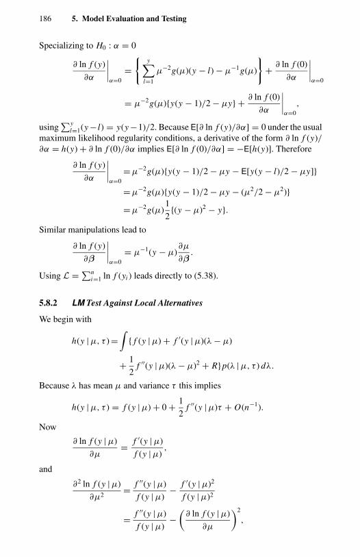
186 5. Model Evaluation and Testing

Specializing to H0 : α = 0

∂ ln f (y)

∂α

∣∣∣∣α=0

=

y∑l=1

µ−2g(µ)(y − l) − µ−1g(µ)

+ ∂ ln f (0)

∂α

∣∣∣∣α=0

= µ−2g(µ)y(y − 1)/2 − µy + ∂ ln f (0)

∂α

∣∣∣∣α=0

,

using∑y

l=1(y − l) = y(y −1)/2. Because E[∂ ln f (y)/∂α] = 0 under the usualmaximum likelihood regularity conditions, a derivative of the form ∂ ln f (y)/∂α = h(y) + ∂ ln f (0)/∂α implies E[∂ ln f (0)/∂α] = −E[h(y)]. Therefore

∂ ln f (y)

∂α

∣∣∣∣α=0

= µ−2g(µ)y(y − 1)/2 − µy − E[y(y − l)/2 − µy]

= µ−2g(µ)y(y − 1)/2 − µy − (µ2/2 − µ2)= µ−2g(µ)

1

2(y − µ)2 − y.

Similar manipulations lead to

∂ ln f (y)

∂β

∣∣∣∣α=0

= µ−1(y − µ)∂µ

∂β.

Using L =∑ni=1 ln f (yi ) leads directly to (5.38).

5.8.2 LM Test Against Local Alternatives

We begin with

h(y | µ, τ ) =∫

f (y | µ) + f ′(y | µ)(λ − µ)

+ 1

2f ′′(y | µ)(λ − µ)2 + Rp(λ | µ, τ ) dλ.

Because λ has mean µ and variance τ this implies

h(y | µ, τ ) = f (y | µ) + 0 + 1

2f ′′(y | µ)τ + O(n−1).

Now

∂ ln f (y | µ)

∂µ= f ′(y | µ)

f (y | µ),

and

∂2 ln f (y | µ)

∂µ2= f ′′(y | µ)

f (y | µ)− f ′(y | µ)2

f (y | µ)2

= f ′′(y | µ)

f (y | µ)−(

∂ ln f (y | µ)

∂µ

)2

,

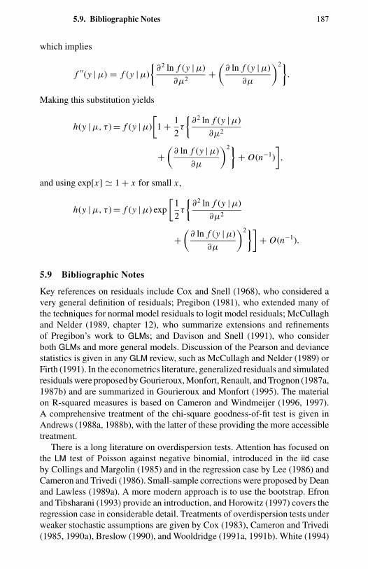
5.9. Bibliographic Notes 187

which implies

f ′′(y | µ) = f (y | µ)

∂2 ln f (y | µ)

∂µ2+(

∂ ln f (y | µ)

∂µ

)2.

Making this substitution yields

h(y | µ, τ ) = f (y | µ)

[1 + 1

2τ

∂2 ln f (y | µ)

∂µ2

+(

∂ ln f (y | µ)

∂µ

)2+ O(n−1)

],

and using exp[x] 1 + x for small x ,

h(y | µ, τ ) = f (y | µ) exp

[1

2τ

∂2 ln f (y | µ)

∂µ2

+(

∂ ln f (y | µ)

∂µ

)2]+ O(n−1).

5.9 Bibliographic Notes

Key references on residuals include Cox and Snell (1968), who considered avery general definition of residuals; Pregibon (1981), who extended many ofthe techniques for normal model residuals to logit model residuals; McCullaghand Nelder (1989, chapter 12), who summarize extensions and refinementsof Pregibon’s work to GLMs; and Davison and Snell (1991), who considerboth GLMs and more general models. Discussion of the Pearson and deviancestatistics is given in any GLM review, such as McCullagh and Nelder (1989) orFirth (1991). In the econometrics literature, generalized residuals and simulatedresiduals were proposed by Gourieroux, Monfort, Renault, and Trognon (1987a,1987b) and are summarized in Gourieroux and Monfort (1995). The materialon R-squared measures is based on Cameron and Windmeijer (1996, 1997).A comprehensive treatment of the chi-square goodness-of-fit test is given inAndrews (1988a, 1988b), with the latter of these providing the more accessibletreatment.

There is a long literature on overdispersion tests. Attention has focused onthe LM test of Poisson against negative binomial, introduced in the iid caseby Collings and Margolin (1985) and in the regression case by Lee (1986) andCameron and Trivedi (1986). Small-sample corrections were proposed by Deanand Lawless (1989a). A more modern approach is to use the bootstrap. Efronand Tibsharani (1993) provide an introduction, and Horowitz (1997) covers theregression case in considerable detail. Treatments of overdispersion tests underweaker stochastic assumptions are given by Cox (1983), Cameron and Trivedi(1985, 1990a), Breslow (1990), and Wooldridge (1991a, 1991b). White (1994)

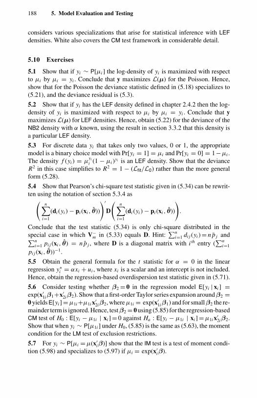
188 5. Model Evaluation and Testing

considers various specializations that arise for statistical inference with LEFdensities. White also covers the CM test framework in considerable detail.

5.10 Exercises

5.1 Show that if yi ∼ P[µi ] the log-density of yi is maximized with respectto µi by µi = yi . Conclude that y maximizes L(µ) for the Poisson. Hence,show that for the Poisson the deviance statistic defined in (5.18) specializes to(5.21), and the deviance residual is (5.3).

5.2 Show that if yi has the LEF density defined in chapter 2.4.2 then the log-density of yi is maximized with respect to µi by µi = yi . Conclude that ymaximizes L(µ) for LEF densities. Hence, obtain (5.22) for the deviance of theNB2 density with α known, using the result in section 3.3.2 that this density isa particular LEF density.

5.3 For discrete data yi that takes only two values, 0 or 1, the appropriatemodel is a binary choice model with Pr[yi = 1] = µi and Pr[yi = 0] = 1−µi .The density f (yi ) = µ

yi

i (1 − µi )yi is an LEF density. Show that the devianceR2 in this case simplifies to R2 = 1 − (Lfit/L0) rather than the more generalform (5.28).

5.4 Show that Pearson’s chi-square test statistic given in (5.34) can be rewrit-ten using the notation of section 5.3.4 as(

n∑i=1

(di (yi ) − pi (xi , θ))

)′D

(n∑

i=1

(di (yi ) − pi (xi , θ))

).

Conclude that the test statistic (5.34) is only chi-square distributed in thespecial case in which V−

m in (5.33) equals D. Hint:∑n

i=1 di j (yi ) = n p j and∑ni=1 pi j (xi , θ) = n p j , where D is a diagonal matrix with i th entry (

∑ni=1

pi j (xi , θ))−1.

5.5 Obtain the general formula for the t statistic for α = 0 in the linearregression y∗

i = αxi + ui , where xi is a scalar and an intercept is not included.Hence, obtain the regression-based overdispersion test statistic given in (5.71).

5.6 Consider testing whether β2 = 0 in the regression model E[yi | xi ] =exp(x′

1iβ1+x′2iβ2). Show that a first-order Taylor series expansion aroundβ2 =

0 yields E[yi ] = µ1i +µ1i x′2iβ2, where µ1i = exp(x′

1iβ1) and for smallβ2 the re-mainder term is ignored. Hence, testβ2 = 0 using (5.85) for the regression-basedCM test of H0 : E[yi − µ1i | xi ] = 0 against Ha : E[yi − µ1i | xi ] = µ1i x′

2iβ2.Show that when yi ∼ P[µ1i ] under H0, (5.85) is the same as (5.63), the momentcondition for the LM test of exclusion restrictions.

5.7 For yi ∼ P[µi = µ(x′iβ)] show that the IM test is a test of moment condi-

tion (5.98) and specializes to (5.97) if µi = exp(x′iβ).

CHAPTER 6

Empirical Illustrations

6.1 Introduction

In this chapter we provide a detailed discussion of empirical models based ontwo cross-sectional data sets. The first of these analyzes the demand for medicalcare by the elderly in the United States. This data set shares many features ofhealth utilization studies based on cross-section data. The second is an analysisof recreational trips.

Section 6.2 extends the introduction by surveying two general modeling is-sues. The first is the decision to model only the conditional mean versus thefull distribution of counts. The second issue concerns behavioral interpretationof count models, an issue of importance to econometricians who emphasizethe distinction between reduced form and structural models. Sections 6.3 and6.4 deal in turn with each of the two empirical applications. Each has severalsubsections that deal with details. The health care example in section 6.3 is in-tended to illustrate in detail the methodology for fitting a finite mixture model.There are relatively few econometric examples that discuss at length the imple-mentation of the finite mixture model and the interpretation of the results. Theexample is intended to fill this gap. Section 6.5 pursues a methodological ques-tion concerning the distribution of the LR test under nonstandard conditions,previously raised in section 4.8.5. The final two sections provide concludingremarks and bibliographic notes.

The emphasis of this chapter is on practical aspects of modeling. Each appli-cation involves several competing models which are compared and evaluatedusing model diagnostics and goodness-of-fit measures. Although the Poissonregression model is the most common starting point in count data analysis, it isusually abandoned in favor of a more general mixed Poisson model. This usu-ally occurs after diagnostic tests reveal overdispersion. But in many cases thismechanical approach can produce misleading results. Overdispersion may be aconsequence of many diverse factors. An empirical model that simply controlsfor overdispersion does not shed any light on its source. Tests of overdispersiondo not unambiguously suggest remedies. This is because they may have poweragainst many commonplace misspecifications. Rejection of the null against a

190 6. Empirical Illustrations

specific alternative does not imply that the alternative itself is valid. Hencemisspecifications and directions for model revision should be explored withcare.

6.2 Background

6.2.1 Fully Parametric Estimation

Event count models may have two different uses. In some cases, the maininterest is in modeling the conditional expectation of the count and in makinginferences about key parameters, such as price elasticity. Different models andestimation methods may yield similar results with respect to the conditionalmean, even though they differ in the goodness of fit.

In other cases, the entire frequency distribution of events is relevant. An in-teresting example is Dionne and Vanasse (1992), where the entire distributionof auto accidents is used to derive insurance-premium tables as a function ofaccident history and individual characteristics. Another example is the proba-bility distribution of number of patient days in hospital as a function of patientcharacteristics. These probabilities might be needed to generate the expectedcosts of hospital stays.

If the objective is to make conditional predictions about the expected num-ber of events, the focus is on the conditional mean function. But if the focusis on the conditional probability of a given number of events, the frequencydistribution itself is relevant. In the former case, features such as overdisper-sion may affect the prediction intervals but not mean prediction. In the lattercase overdispersion will affect the estimated cell probability. Hence, parametricmethods are attractive in the latter case, whereas robustness of the estimate ismore important in the former.

This neat separation of modeling issues is not possible, however, if con-sistent estimation of the conditional expectation also requires fully parametricmodels. For example, the conditional mean may correspond to that for theZIP or Poisson hurdle model, in which case one needs to model the probabili-ties. Chapter 3 focused on methods by which other aspects of the distribution,notably the variance, are modeled to improve efficiency. Chapter 4, in con-trast, presents many parametric models in which consistent estimation of theconditional mean parameters requires fully parametric methods. The attentiongiven to features such as variance function modeling varies on a case-by-casebasis.

To make the foregoing discussion concrete, consider the issue of how to treatthe joint presence of excess zero observations and long right tails relative tothe Poisson regression. One interpretation of this condition is that it indicatesunobserved heterogeneity. Hence, it is a problem of modeling the variance func-tion. The Two-Crossings Theorem supports this interpretation. An alternativeinterpretation is that the excess zeros reflect behavior. Many individuals donot record (experience) positive counts because they do not “participate” in a

6.2. Background 191

relevant activity. That is, optimizing behavior generates corner solutions. Onthis interpretation, the presence of excess zeros may well be a feature of theconditional mean function, not the variance function. If one adds to this thepresence of unobserved heterogeneity, it is concluded that both the conditionalexpectation and variance function are involved. So the use of an overdispersedPoisson model, such as the negative binomial, without also allowing for theadditional nonlinearity generated by an excess of corner solutions, yields in-consistent estimates of the parameters.

6.2.2 Repeated Events

Consider a single probabilistic event such as the desire for a recreational tripor the number of spells of sickness. That may or may not lead to the outcomeof interest, such as a doctor visit or a recreational trip. If the outcome reflectsindividual decision making, it may be analyzed within the random utility frame-work used in binary choice models. Suppose we consider a doctor consultation.Denote by U0 the utility of not seeking care and by U1 the utility of seekingcare. Both U0 and U1 are latent variables. Let

U1i = x′iβ1 + ε1i

U0i = x′iβ0 + ε0i ,

where xi is the vector of individual attributes, and ε1i and ε0i are random errors.Then for individual i who seeks care, we have

U1i > U0i ⇒ ε0i − ε1i < x′i (β1 − β0).

Thus, the probability of the decision to seek care is characterized by the standardbinary outcome model. The individual i seeks care if U1i > U0i , and we observey = 1. Otherwise we observe y = 0. The probability of y = 1, denoted π , isgiven by Pr [ε0i − ε1i < x′

i (β1 − β0)].Next consider repeated events of the same kind. If there is a fixed number,

N , of repetitions, the event distribution is binomial B(N , p). Suppose, how-ever, that N is random and follows Poisson distribution. For simplicity treatthe events as N independent Bernoulli trials occurring over some time inter-val. By the application of the Poisson-stopped binomial result, the numberof successes is Poisson-distributed (see Chapter 1). This argument justifies theframework of count-data models for the study of repeated events based on eventcounts.

This argument can be generalized in a straightforward manner to allow forserial correlation of events or unobserved heterogeneity, both of which implyoverdispersion. The framework also generalizes to the multinomial case inwhich the observed event is one of k outcomes. For example, the individualmay choose to visit any one of k possible recreational sites, and such a choiceoutcome may be repeated a random number of times.

192 6. Empirical Illustrations

6.3 Analysis of Demand for Health Services

Count models are extensively used in modeling healthcare utilization. Discretemeasures of units of healthcare use are often more easily available than dataon expenditures. They are usually obtained from national health or health ex-penditure surveys, which also provide information on key covariates such asmeasures of health insurance, health status, income, education, and many so-ciodemographic variables.

This example draws on Deb and Trivedi (1997), which deals with counts ofmedical care utilization. The article compares the performance of a negativebinomial (NB), two-part hurdles negative binomial (NBH), and finite mixturenegative binomial (FMNB) in a study of the demand for medical care by theelderly aged 66 years and over in the United States, using six mutually exclusivemeasures of utilization.

6.3.1 Health Service Data

A sample of 4406 cases was obtained from the National Medical ExpenditureSurvey conducted in 1987 and 1988 (NMES). The data provide a comprehensivepicture of how Americans use and pay for health services. Here only one ofthese six measures, that dealing with the office visits to physicians (OFP), isconsidered. A feature of these data is that they do not include a high proportionof zero counts but do reflect a high degree of unconditional overdispersion.

The NMES is based on a representative, national probability sample of thecivilian, noninstitutionalized population and individuals admitted to long-termcare facilities during 1987. Under the household survey of the NMES, morethan 38,000 individuals in 15,000 households across the United States wereinterviewed quarterly about their health insurance coverage, the services theyused, and the cost and source of payments of those services. In addition tohealthcare data, NMES provides information on health status, employment,sociodemographic characteristics, and economic status.

An important issue in healthcare modeling is endogeneity of health insur-ance. If consumers make their decisions on health insurance and healthcareutilization jointly, then the two are stochastically dependent. Hence, health in-surance status should not be treated as a valid exogenous variable. We firstconsider the argument of Deb and Trivedi (1997) that for the elderly U.S. popu-lation it is reasonable to take health insurance status as an exogenous covariate.

All cases in the sample were covered by Medicare, a public insurance pro-gram that offers substantial protection against healthcare costs. Residents ofthe United States are eligible for Medicare coverage at age 65 years. Someindividuals start receiving Medicare benefits a few months into their 65th yearprimarily because they fail to apply for coverage at the appropriate time. Virtu-ally all individuals who are 66 years of age or older are covered by Medicare.In addition, most individuals make a choice of supplemental private insurancecoverage shortly before or in their 65th year because the price of such insurance

6.3. Analysis of Demand for Health Services 193

Table 6.1. OFP visits: actual frequency distribution

Number of visits 0 1 2 3 4 5 6 7 8 9 10 11 12 13+Frequency 683 481 428 420 383 338 268 217 188 171 128 115 86 500

rises sharply with age and coverage becomes more restrictive. Therefore, giventhe choice of sample, the treatment of private insurance status as predetermined,rather than endogenous, is justified. On the other hand, to the extent that privateinsurance purchase is in anticipation of required healthcare, given health status,private insurance status may be treated as endogenous. Because the specificationcontrols for health status by including several health status variables, the forceof this argument is reduced. Exogeneity of insurance is a major econometricsimplification.

The frequency distribution of physician office visits is given in Table 6.1.The zero counts account for only about 15% of the visits. There is a long righttail. Around 11% of the patients have 13 or more visits. Definitions and sum-mary statistics for the explanatory variables are presented in Table 6.2. Thehealth measures include self-perceived measures of health (EXCLHLTH andPOORHLTH ), the number of chronic diseases and conditions (NUMCHRON )and a measure of disability status (ADLDIFF ). In order to control for regionaldifferences we use NOREAST, MIDWEST, and WEST. The demographic vari-ables include AGE, race (BLACK ), sex (MALE ), marital status (MARRIED),and education (SCHOOL). Finally, the economic variables are family income(FAMINC ), employment status (EMPLOY ), supplementary private insurancestatus (PRIVINS ), and public insurance status (MEDICAID). Medicaid, whichshould not be confused with Medicare, is available to low-income individu-als only. Both PRIVINS and MEDICAID serve as indicators of the price ofservice.

6.3.2 Demand for Medical Care

Beginning with the obvious starting point of the Poisson regression is unneces-sary. The data display a high degree of overdispersion, leading to the rejectionof the Poisson model. Even the NB1 and NB2 models are easily rejected by thechi-squared goodness-of-fit test, suggesting that the conditional mean may bemisspecified.

Several recent studies have suggested that the two-part hurdle model pro-vides a better starting point than the NB class. The two-part hurdle model hasperformed satisfactorily in several empirical studies (Pohlmeier and Ulrich,1995; Gurmu, 1997; Geil et al., 1997) of health utilization. It is typically supe-rior to specifications in which the two separate origins of zero observations arenot recognized. It may be interpreted as a principal-agent type model in whichthe first part specifies the decision to seek care as a binary outcome process,

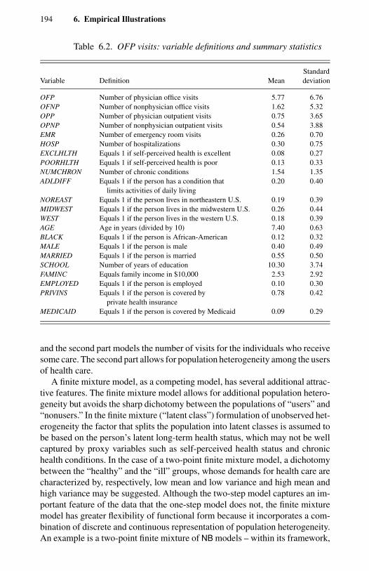
194 6. Empirical Illustrations

Table 6.2. OFP visits: variable definitions and summary statistics

StandardVariable Definition Mean deviation

OFP Number of physician office visits 5.77 6.76OFNP Number of nonphysician office visits 1.62 5.32OPP Number of physician outpatient visits 0.75 3.65OPNP Number of nonphysician outpatient visits 0.54 3.88EMR Number of emergency room visits 0.26 0.70HOSP Number of hospitalizations 0.30 0.75EXCLHLTH Equals 1 if self-perceived health is excellent 0.08 0.27POORHLTH Equals 1 if self-perceived health is poor 0.13 0.33NUMCHRON Number of chronic conditions 1.54 1.35ADLDIFF Equals 1 if the person has a condition that 0.20 0.40

limits activities of daily livingNOREAST Equals 1 if the person lives in northeastern U.S. 0.19 0.39MIDWEST Equals 1 if the person lives in the midwestern U.S. 0.26 0.44WEST Equals 1 if the person lives in the western U.S. 0.18 0.39AGE Age in years (divided by 10) 7.40 0.63BLACK Equals 1 if the person is African-American 0.12 0.32MALE Equals 1 if the person is male 0.40 0.49MARRIED Equals 1 if the person is married 0.55 0.50SCHOOL Number of years of education 10.30 3.74FAMINC Equals family income in $10,000 2.53 2.92EMPLOYED Equals 1 if the person is employed 0.10 0.30PRIVINS Equals 1 if the person is covered by 0.78 0.42

private health insuranceMEDICAID Equals 1 if the person is covered by Medicaid 0.09 0.29

and the second part models the number of visits for the individuals who receivesome care. The second part allows for population heterogeneity among the usersof health care.

A finite mixture model, as a competing model, has several additional attrac-tive features. The finite mixture model allows for additional population hetero-geneity but avoids the sharp dichotomy between the populations of “users” and“nonusers.” In the finite mixture (“latent class”) formulation of unobserved het-erogeneity the factor that splits the population into latent classes is assumed tobe based on the person’s latent long-term health status, which may not be wellcaptured by proxy variables such as self-perceived health status and chronichealth conditions. In the case of a two-point finite mixture model, a dichotomybetween the “healthy” and the “ill” groups, whose demands for health care arecharacterized by, respectively, low mean and low variance and high mean andhigh variance may be suggested. Although the two-step model captures an im-portant feature of the data that the one-step model does not, the finite mixturemodel has greater flexibility of functional form because it incorporates a com-bination of discrete and continuous representation of population heterogeneity.An example is a two-point finite mixture of NB models – within its framework,

6.3. Analysis of Demand for Health Services 195

one might view a population of healthcare consumers as consisting of discrete“types” (ill and healthy) and yet allow for heterogeneity within each type.

6.3.3 Competing Models

Three models are compared. The first is the NB model with mean E[yi | xi ] =µi = exp(x′

iβ) and variance V[yi | xi ] = µi + αµpi where α > 0 is an overdis-

persion parameter. The NB1 model is obtained by specifying p = 1; NB2 isobtained by setting p = 2.∗

The second is the NBH, which has the following components:

Prh[yi = 0 | xi ] =(

ψh,i

µh,i + ψh,i

)ψh,i

, (6.1)

Pr [yi > 0 | xi ] = 1 −(

ψi

µi + ψi

)ψi

, (6.2)

where the subscript h refers to the hurdle distribution and ψi = (1/α)µ2−pi .

This is introduced in section 4.7. In the NBH model, the mean of the countvariable is given by

E[yi | xi ] = Prh[yi > 0 | xi ]

Pr [yi > 0 | xi ]µi (6.3)

and the variance by

V[yi | xi ] = Prh[yi > 0 | xi ]

Pr [yi > 0 | xi ]

[µi + αµ

pi +(

1 − Prh[yi > 0 | xi ]

Pr [yi > 0 | xi ]

)µ2

i

].

(6.4)

The third model is the C-component finite mixture density specified as fol-lows:

f (yi |Θ) =C−1∑j=1

πj fj (yi |θj ) + πC fC (yi |θC ), (6.5)

where π1 ≥ π2 ≥ · · · · ≥ πC , πC = (1−∑C−1j=1 πj ) are the mixing probabilities

(proportions of the sampled latent subpopulations) estimated along with allother parameters, all collectively denoted by Θ; see section 4.8. The componentdistributions in a C-point FMNB model (FMNB-C) are specified as

fj (yi ) = (yi + ψj,i )

(ψj,i )(yi + 1)

(ψj,i

µj,i + ψj,i

)ψ j,i(

µ j,i

µ j,i + ψj,i

)yi

.

(6.6)

∗ This notation is slightly different from Chapter 3, where the notation is V[yi | xi ] = µi + αµpi ,

with p = 1 yielding NB1 and p = 2 yielding NB2.

196 6. Empirical Illustrations

A variant of the third model constrains slope coefficients to be equal. Ifdim[βj ] = k, then the fully unconstrained C component mixture has dimen-sion C(k + 1) − 1. The models in the current application become possiblyoverparameterized when k is around 10. Hence considerations of parsimoniousparameterization motivate restrictions across the component densities. There-fore Deb and Trivedi (1997) also considered a constrained FMNB-C (CFMNB-C)in which all slope parameters in βj were restricted to be equal across all C com-ponents. The differences between component distributions then arise only fromintercept differences.

The slope-constrained, or random intercept, model is the same as the dis-crete specification of heterogeneity used in Simar (1976), Laird (1978), Lindsay(1995), and Heckman and Singer (1984). This specification is relatively par-simonious and, as discussed in Chapter 4, may provide an adequate semi- ornonparametric representation of the possibly continuous distribution of unob-served heterogeneity.

It is interesting that the CFMNB-C may be consistently estimated, up to theintercept, by Poisson maximum likelihood. This follows from the exponentialmean function E[yi | xi ]. For example, with C = 2,

E[yi | xi ] = exp[πβ01 + (1 − π )β02 + x′

iβ].

The intercept of the constrained finite mixture is a weighted sum of the interceptsin the components, with weights being the population proportions π and 1−π .Hence, Poisson maximum likelihood yields only an estimate of the weightedsum of the intercepts and not the individual components that we need in orderto estimate subpopulation means.

6.3.4 Is There a Mixture?

There are two important issues in evaluating fitted finite mixture models. First,is there evidence for the presence of more than one components? That is, ismixing present? Second, is a global maximum attained in estimation?

Lindsay and Roeder (1992) have developed diagnostic tools for checkingthese properties for the case of exponential mixtures. The key idea behind thediagnostic for the presence of a mixture component is the Two Crossings Theo-rem given in section 4.2. Let p(y;θ∗) denote fitted-cell probabilities calculatedunder the assumption that the data are generated by a one-component model,and let p(y; C) denote the fitted probability based on the assumption that thesample comes from a C-component mixture distribution. Then by an extensionof Shaked’s Two Crossings Theorem, the differences ( p(y;θ∗)− p(y; C)) showa +, −, + sign pattern. This is the basis of the first of two diagnostic toolsdeveloped by Lindsay and Roeder. Their directional gradient function is

d(y, C,θ∗) =(

p(y;θ∗)

p(y; C)− 1

), y = 0, 1, 2, . . . , (6.7)

6.3. Analysis of Demand for Health Services 197

where θ∗ is the unicomponent MLE and C is the C-component MLE. To calcu-late d(y, C,θ∗) we first calculate d(yi , C,θ∗ | xi ) and then average across allobservations. The convexity of the graph of d(y, C,θ∗) against y is interpretedas evidence in favor of a mixture. However, note that such convexity may beobserved for more than one value of C , leaving open the issue of which valueto select for C .

Lindsay and Roeder also suggest the use of the weighted sum measure

D(C,θ∗) =∑y∈S

d(y, C,θ∗)p(y) (6.8)

as an additional diagnostic. This can be interpreted as a quantitative measure ofthe deviation in fitted cell probabilities induced by the mixture. A limitation ofthis statistic is that in the event of a long right tail, the contribution of high valuesof y may be large. This tends to make the components of D(C,θ∗) erratic, andthe statistic itself may be hard to interpret. Recognizing this feature, Lindsayand Roeder suggest that a truncated gradient statistic is preferred for unboundeddensities. However, currently there is little guidance on how the statistic shouldbe truncated.

The diagnostic tools of Lindsay and Roeder are intended for exponentialmixtures. Strictly speaking, they should not be used for the negative binomialmixture.∗ In this chapter these tools are applied in a heuristic and exploratoryfashion to the FMNB-C model.

6.3.5 Model Comparison and Selection

Given the presence of mixture, one may either sequentially compare modelswith different values of C or compare unconstrained and constrained modelsfor a given C . Although these are both nested hypotheses, the use of the LRtest is only appropriate for the latter simplification, not the former in which thehypothesis is on the boundary of the parameter space. This violates the standardregularity conditions for maximum likelihood. For example, in a model with nocomponent-density parameters estimated, the LR test of the null hypothesis H0 :πC = 0 versus Ha : πC = 0 does not have the usual null χ2(1) distribution. In-stead, the asymptotic distribution of the likelihood ratio is a weighted chi-square.

Bohning et al. (1994) have used simulation analysis to examine the distribu-tion of the LR test for several distributions involving a boundary hypothesis. Thisshowed that the use of the nominal χ2(1) test is likely to underreject the falsenull. Therefore, systematic reliance on the LR test may cause an investigator tochoose a value of C that is too small. However, the use of information crite-ria – we use the AIC and the BIC – for model selection has formal justification.Leroux (1992) proves that under regularity conditions the maximum penalized

∗ Note, however, that the two-crossings result is extended to two-parameter exponential familiesby Gelfand and Dalal (1990).

198 6. Empirical Illustrations

likelihood approach, for example the use of the AIC-BIC, leads to a consistentestimator of the true finite-mixture model (Leroux, 1992, section 3.3). Section6.4 provides a further discussion of these issues using simulation evidence.

Model simplification in going from NBH to NB involves a standard nestedhypothesis; therefore, it may be based on the LR test. Finally, if FMNB-C,C > 1, and NBH are the preferred models after initial tests, one should selectbetween these two. Note that FMNB-1 means NB and NB may refer to eitherNB1 or NB2. Again this involves nonnested comparisons, for which we useinformation criteria to choose between them.

A possible strategy for model selection can be summarized as follows:

• Fix maximum C = C∗. Use information criteria to compare the se-quence of models FMNB-C∗, . . . ., FMNB-1.

• Use the LR test to compare FMNB-C and CFMNB-C.• Use the LR test to compare NBH and NB.• Use information criteria to compare FMNB-C (or CFMNB-C) and NBH.

Finally, to evaluate the goodness of fit of the model selected after this mul-tilevel comparison of models, one may use the chi-square diagnostic test intro-duced in section 5.3.4. This compares actual and fitted cell frequencies of eventsfor which cells are centered on integer values. The fitted cell frequencies arecalculated as follows. Let pi j , i = 1, 2, . . . , N ; y = 0, 1, 2, . . . , denote the fit-ted probability that individual i experiences j events. Then the fitted frequencyin cell j is calculated as n p j , where

p j = 1

n

∑i

pi j , j = 0, 1, 2, . . . . (6.9)

In the present case, the chi-square goodness-of-fit statistic is

TGoF = (f − f )′V−1(f − f ) (6.10)

where f − f is the q dimensional vector of difference between sample and fittedcell frequencies, q is the number of cells used in the test, and V is the estimatedvariance matrix of the difference; see Chapter 5.3. Under the null hypothesisof no misspecification the test has an asymptotic χ2(q − 1) distribution. Inmost cases the last cell aggregates over several sample support points. If thesample mean is low, then fewer support points are used than if the value islarge. For computational simplicity, the covariance matrix of f − f is estimatedby an auxiliary regression based on the outer product of gradients as discussedin Andrews (1988b, Appendix 5).

Be aware that the proposed model comparison and selection approach issubject to the usual criticism that there will be pre-test bias resulting from thechoices. Hence, if the data availability permits, the above approach should beused on a training sample and the selected model should be reestimated usingnew data.

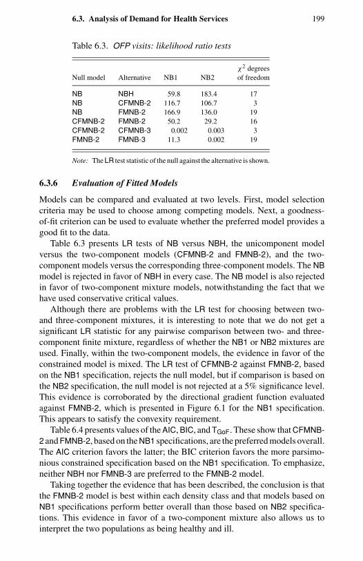
6.3. Analysis of Demand for Health Services 199

Table 6.3. OFP visits: likelihood ratio tests

χ2 degreesNull model Alternative NB1 NB2 of freedom

NB NBH 59.8 183.4 17NB CFMNB-2 116.7 106.7 3NB FMNB-2 166.9 136.0 19CFMNB-2 FMNB-2 50.2 29.2 16CFMNB-2 CFMNB-3 0.002 0.003 3FMNB-2 FMNB-3 11.3 0.002 19

Note: The LR test statistic of the null against the alternative is shown.

6.3.6 Evaluation of Fitted Models

Models can be compared and evaluated at two levels. First, model selectioncriteria may be used to choose among competing models. Next, a goodness-of-fit criterion can be used to evaluate whether the preferred model provides agood fit to the data.

Table 6.3 presents LR tests of NB versus NBH, the unicomponent modelversus the two-component models (CFMNB-2 and FMNB-2), and the two-component models versus the corresponding three-component models. The NBmodel is rejected in favor of NBH in every case. The NB model is also rejectedin favor of two-component mixture models, notwithstanding the fact that wehave used conservative critical values.

Although there are problems with the LR test for choosing between two-and three-component mixtures, it is interesting to note that we do not get asignificant LR statistic for any pairwise comparison between two- and three-component finite mixture, regardless of whether the NB1 or NB2 mixtures areused. Finally, within the two-component models, the evidence in favor of theconstrained model is mixed. The LR test of CFMNB-2 against FMNB-2, basedon the NB1 specification, rejects the null model, but if comparison is based onthe NB2 specification, the null model is not rejected at a 5% significance level.This evidence is corroborated by the directional gradient function evaluatedagainst FMNB-2, which is presented in Figure 6.1 for the NB1 specification.This appears to satisfy the convexity requirement.

Table 6.4 presents values of the AIC, BIC, and TGoF. These show that CFMNB-2 and FMNB-2, based on the NB1 specifications, are the preferred models overall.The AIC criterion favors the latter; the BIC criterion favors the more parsimo-nious constrained specification based on the NB1 specification. To emphasize,neither NBH nor FMNB-3 are preferred to the FMNB-2 model.

Taking together the evidence that has been described, the conclusion is thatthe FMNB-2 model is best within each density class and that models based onNB1 specifications perform better overall than those based on NB2 specifica-tions. This evidence in favor of a two-component mixture also allows us tointerpret the two populations as being healthy and ill.

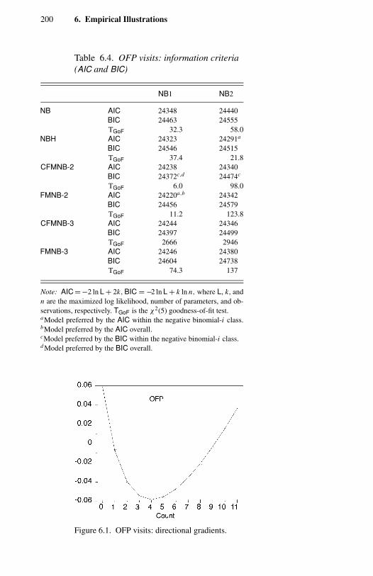
200 6. Empirical Illustrations

Table 6.4. OFP visits: information criteria(AIC and BIC)

NB1 NB2

NB AIC 24348 24440BIC 24463 24555TGoF 32.3 58.0

NBH AIC 24323 24291a

BIC 24546 24515TGoF 37.4 21.8

CFMNB-2 AIC 24238 24340BIC 24372c,d 24474c

TGoF 6.0 98.0FMNB-2 AIC 24220a,b 24342

BIC 24456 24579TGoF 11.2 123.8

CFMNB-3 AIC 24244 24346BIC 24397 24499TGoF 2666 2946

FMNB-3 AIC 24246 24380BIC 24604 24738TGoF 74.3 137

Note: AIC = −2 ln L + 2k, BIC = −2 ln L + k ln n, where L, k, andn are the maximized log likelihood, number of parameters, and ob-servations, respectively. TGoF is the χ2(5) goodness-of-fit test.aModel preferred by the AIC within the negative binomial-i class.bModel preferred by the AIC overall.cModel preferred by the BIC within the negative binomial-i class.d Model preferred by the BIC overall.

Figure 6.1. OFP visits: directional gradients.

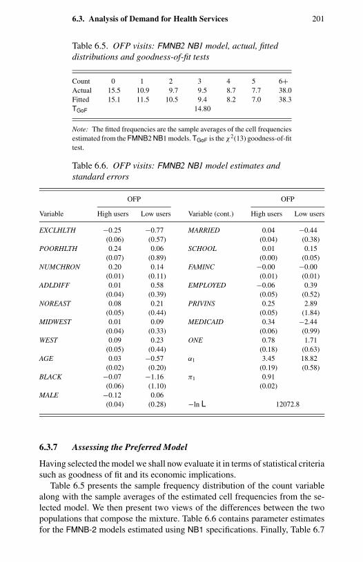
6.3. Analysis of Demand for Health Services 201

Table 6.5. OFP visits: FMNB2 NB1 model, actual, fitteddistributions and goodness-of-fit tests

Count 0 1 2 3 4 5 6+Actual 15.5 10.9 9.7 9.5 8.7 7.7 38.0Fitted 15.1 11.5 10.5 9.4 8.2 7.0 38.3TGoF 14.80

Note: The fitted frequencies are the sample averages of the cell frequenciesestimated from the FMNB2 NB1 models. TGoF is the χ2(13) goodness-of-fittest.

Table 6.6. OFP visits: FMNB2 NB1 model estimates andstandard errors

OFP OFP

Variable High users Low users Variable (cont.) High users Low users

EXCLHLTH −0.25 −0.77 MARRIED 0.04 −0.44(0.06) (0.57) (0.04) (0.38)

POORHLTH 0.24 0.06 SCHOOL 0.01 0.15(0.07) (0.89) (0.00) (0.05)

NUMCHRON 0.20 0.14 FAMINC −0.00 −0.00(0.01) (0.11) (0.01) (0.01)

ADLDIFF 0.01 0.58 EMPLOYED −0.06 0.39(0.04) (0.39) (0.05) (0.52)

NOREAST 0.08 0.21 PRIVINS 0.25 2.89(0.05) (0.44) (0.05) (1.84)

MIDWEST 0.01 0.09 MEDICAID 0.34 −2.44(0.04) (0.33) (0.06) (0.99)

WEST 0.09 0.23 ONE 0.78 1.71(0.05) (0.44) (0.18) (0.63)

AGE 0.03 −0.57 α1 3.45 18.82(0.02) (0.20) (0.19) (0.58)

BLACK −0.07 −1.16 π1 0.91(0.06) (1.10) (0.02)

MALE −0.12 0.06(0.04) (0.28) −ln L 12072.8

6.3.7 Assessing the Preferred Model

Having selected the model we shall now evaluate it in terms of statistical criteriasuch as goodness of fit and its economic implications.

Table 6.5 presents the sample frequency distribution of the count variablealong with the sample averages of the estimated cell frequencies from the se-lected model. We then present two views of the differences between the twopopulations that compose the mixture. Table 6.6 contains parameter estimatesfor the FMNB-2 models estimated using NB1 specifications. Finally, Table 6.7

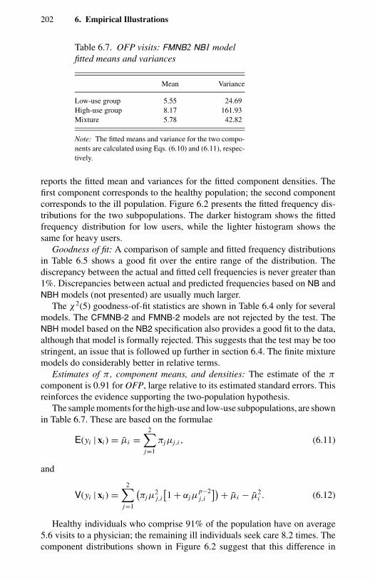
202 6. Empirical Illustrations

Table 6.7. OFP visits: FMNB2 NB1 modelfitted means and variances

Mean Variance

Low-use group 5.55 24.69High-use group 8.17 161.93Mixture 5.78 42.82

Note: The fitted means and variance for the two compo-nents are calculated using Eqs. (6.10) and (6.11), respec-tively.

reports the fitted mean and variances for the fitted component densities. Thefirst component corresponds to the healthy population; the second componentcorresponds to the ill population. Figure 6.2 presents the fitted frequency dis-tributions for the two subpopulations. The darker histogram shows the fittedfrequency distribution for low users, while the lighter histogram shows thesame for heavy users.

Goodness of fit: A comparison of sample and fitted frequency distributionsin Table 6.5 shows a good fit over the entire range of the distribution. Thediscrepancy between the actual and fitted cell frequencies is never greater than1%. Discrepancies between actual and predicted frequencies based on NB andNBH models (not presented) are usually much larger.

The χ2(5) goodness-of-fit statistics are shown in Table 6.4 only for severalmodels. The CFMNB-2 and FMNB-2 models are not rejected by the test. TheNBH model based on the NB2 specification also provides a good fit to the data,although that model is formally rejected. This suggests that the test may be toostringent, an issue that is followed up further in section 6.4. The finite mixturemodels do considerably better in relative terms.

Estimates of π , component means, and densities: The estimate of the π

component is 0.91 for OFP, large relative to its estimated standard errors. Thisreinforces the evidence supporting the two-population hypothesis.

The sample moments for the high-use and low-use subpopulations, are shownin Table 6.7. These are based on the formulae

E(yi | xi ) = µi =2∑

j=1

πjµj,i , (6.11)

and

V(yi | xi ) =2∑

j=1

(πjµ

2j,i

[1 + αjµ

p−2j,i

])+ µi − µ2i . (6.12)

Healthy individuals who comprise 91% of the population have on average5.6 visits to a physician; the remaining ill individuals seek care 8.2 times. Thecomponent distributions shown in Figure 6.2 suggest that this difference in

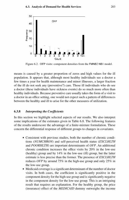
6.3. Analysis of Demand for Health Services 203

Figure 6.2. OFP visits: component densities from the FMNB2 NB1 model.

means is caused by a greater proportion of zeros and high values for the illpopulation. It appears that, although most healthy individuals see a doctor afew times a year for health maintenance and minor illnesses, a larger fractionof the ill do not seek any (preventive?) care. Those ill individuals who do seea doctor (these individuals have sickness events) do so much more often thanhealthy individuals. Because preventive care usually takes the form of a visit toa doctor in an office setting, one would not expect such a pattern of differencesbetween the healthy and ill to arise for the other measures of utilization.

6.3.8 Interpreting the Coefficients

In this section we highlight selected aspects of our results. We also interpretsome implications of the estimates given in Table 6.8. The following featuresof the results underscore the advantage of a finite-mixture formulation. Theseconcern the differential response of different groups to changes in covariates.

• Consistent with previous studies, both the number of chronic condi-tions (NUMCHRON) and self-perceived health status (EXCLHLTHand POORHLTH) are important determinants of OFP. An additionalchronic condition increases the office visits by 20% in the low-use(healthy) group and by 14% in the low-use (ill) group, but the latterestimate is less precise than the former. The presence of EXCLHLTHreduces OFP by around 75% in the high-use group and only 25% inthe low-use group.

• Medicaid coverage is a significant determinant of the number of doctorvisits. In both cases, the coefficient is significantly positive in thecomponent density for the high-use group and is significantly negativein the component density for the low-use group. This is an intriguingresult that requires an explanation. For the healthy group, the price(insurance) effect of the MEDICAID dummy outweighs the income

204 6. Empirical Illustrations

Table 6.8. OFP visits: NB2 hurdle model estimatesand t ratios

Zeros Positives

Variable Coefficient |t | Coefficient |t |

EXCLHLTH −0.330 2.36 −0.377 4.32POORHLTH 0.070 0.40 0.331 5.79NUMCHRON 0.556 10.43 0.143 10.51ALDIFF −0.187 −1.35 0.129 2.44NOREAST 0.130 1.03 0.103 1.96MIDWEST 0.102 0.86 −0.015 0.32WEST 0.204 1.49 0.123 2.42AGE 0.190 2.02 −0.075 1.61BLACK −0.326 2.36 0.001 0.01MALE −0.464 4.54 0.004 0.09MARRIED 0.247 2.18 −0.092 1.99SCHOOL 0.054 4.08 0.021 3.66FAMINC 0.006 0.36 −0.002 −0.37EMPLOYED −0.011 −0.07 0.029 0.39PRIVINS 0.761 6.14 0.221 3.82MEDICAID 0.550 2.96 0.184 2.69ONE −1.471 1.92 1.630 4.07α 0.743 18.40−ln L 12110TGoF 21.86

effect because Medicaid is a health insurance plan for the poor. Butfor poor individuals within the low-use group the opportunity cost ofseeking care is disproportionately large relative to the money price ofcare. This may induce them to seek care less often even though theyhave Medicaid insurance coverage.

• Persons with supplementary private insurance seek care from physi-cians in office more often than individuals without supplementary cov-erage. The usage for OFP is estimated to be nearly 10 times higher forthe high-use group than the low-use group. For the former, PRIVINShas a coefficient of 2.89 as compared with only 0.25 for the low-usegroup. OFP is insensitive to marginal changes in price given the smallbaseline price levels.

• Income effect on OFP usage is negligible. The family income variable(FAMINC) does not affect OFP. Furthermore, EMPLOYED, whichmay capture income effects also, is never significant. One explanationfor the negligible income effect is that the overall generosity of Medi-care irrespective of family income, combined with Social Securityincome, which guarantees a certain level of income, makes utilizationinsensitive to marginal changes in income.

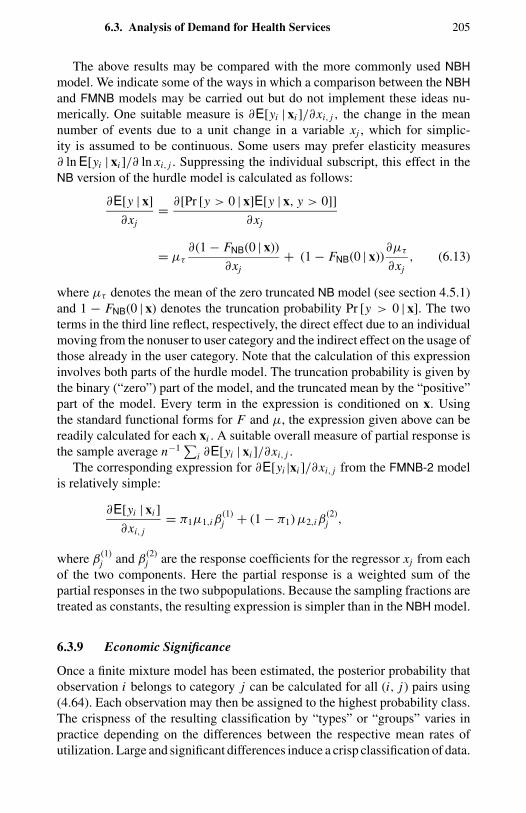
6.3. Analysis of Demand for Health Services 205

The above results may be compared with the more commonly used NBHmodel. We indicate some of the ways in which a comparison between the NBHand FMNB models may be carried out but do not implement these ideas nu-merically. One suitable measure is ∂E[yi | xi ]/∂xi, j , the change in the meannumber of events due to a unit change in a variable xj , which for simplic-ity is assumed to be continuous. Some users may prefer elasticity measures∂ ln E[yi | xi ]/∂ ln xi, j . Suppressing the individual subscript, this effect in theNB version of the hurdle model is calculated as follows:

∂E[y | x]

∂xj= ∂[Pr [y > 0 | x]E[y | x, y > 0]]

∂xj

= µτ

∂(1 − FNB(0 | x))

∂xj+ (1 − FNB(0 | x))

∂µτ

∂xj, (6.13)

where µτ denotes the mean of the zero truncated NB model (see section 4.5.1)and 1 − FNB(0 | x) denotes the truncation probability Pr [y > 0 | x]. The twoterms in the third line reflect, respectively, the direct effect due to an individualmoving from the nonuser to user category and the indirect effect on the usage ofthose already in the user category. Note that the calculation of this expressioninvolves both parts of the hurdle model. The truncation probability is given bythe binary (“zero”) part of the model, and the truncated mean by the “positive”part of the model. Every term in the expression is conditioned on x. Usingthe standard functional forms for F and µ, the expression given above can bereadily calculated for each xi . A suitable overall measure of partial response isthe sample average n−1∑

i ∂E[yi | xi ]/∂xi, j .

The corresponding expression for ∂E[yi |xi ]/∂xi, j from the FMNB-2 modelis relatively simple:

∂E[yi | xi ]

∂xi, j= π1µ1,iβ

(1)j + (1 − π1) µ2,iβ

(2)j ,

where β(1)j and β

(2)j are the response coefficients for the regressor xj from each

of the two components. Here the partial response is a weighted sum of thepartial responses in the two subpopulations. Because the sampling fractions aretreated as constants, the resulting expression is simpler than in the NBH model.

6.3.9 Economic Significance

Once a finite mixture model has been estimated, the posterior probability thatobservation i belongs to category j can be calculated for all (i, j) pairs using(4.64). Each observation may then be assigned to the highest probability class.The crispness of the resulting classification by “types” or “groups” varies inpractice depending on the differences between the respective mean rates ofutilization. Large and significant differences induce a crisp classification of data.

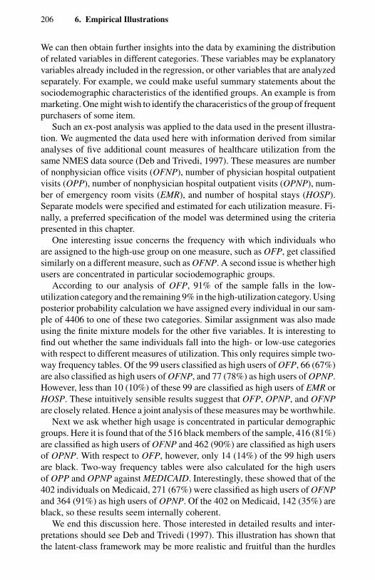
206 6. Empirical Illustrations

We can then obtain further insights into the data by examining the distributionof related variables in different categories. These variables may be explanatoryvariables already included in the regression, or other variables that are analyzedseparately. For example, we could make useful summary statements about thesociodemographic characteristics of the identified groups. An example is frommarketing. One might wish to identify the characeristics of the group of frequentpurchasers of some item.

Such an ex-post analysis was applied to the data used in the present illustra-tion. We augmented the data used here with information derived from similaranalyses of five additional count measures of healthcare utilization from thesame NMES data source (Deb and Trivedi, 1997). These measures are numberof nonphysician office visits (OFNP), number of physician hospital outpatientvisits (OPP), number of nonphysician hospital outpatient visits (OPNP), num-ber of emergency room visits (EMR), and number of hospital stays (HOSP).Separate models were specified and estimated for each utilization measure. Fi-nally, a preferred specification of the model was determined using the criteriapresented in this chapter.

One interesting issue concerns the frequency with which individuals whoare assigned to the high-use group on one measure, such as OFP, get classifiedsimilarly on a different measure, such as OFNP. A second issue is whether highusers are concentrated in particular sociodemographic groups.

According to our analysis of OFP, 91% of the sample falls in the low-utilization category and the remaining 9% in the high-utilization category. Usingposterior probability calculation we have assigned every individual in our sam-ple of 4406 to one of these two categories. Similar assignment was also madeusing the finite mixture models for the other five variables. It is interesting tofind out whether the same individuals fall into the high- or low-use categorieswith respect to different measures of utilization. This only requires simple two-way frequency tables. Of the 99 users classified as high users of OFP, 66 (67%)are also classified as high users of OFNP, and 77 (78%) as high users of OPNP.However, less than 10 (10%) of these 99 are classified as high users of EMR orHOSP. These intuitively sensible results suggest that OFP, OPNP, and OFNPare closely related. Hence a joint analysis of these measures may be worthwhile.

Next we ask whether high usage is concentrated in particular demographicgroups. Here it is found that of the 516 black members of the sample, 416 (81%)are classified as high users of OFNP and 462 (90%) are classified as high usersof OPNP. With respect to OFP, however, only 14 (14%) of the 99 high usersare black. Two-way frequency tables were also calculated for the high usersof OPP and OPNP against MEDICAID. Interestingly, these showed that of the402 individuals on Medicaid, 271 (67%) were classified as high users of OFNPand 364 (91%) as high users of OPNP. Of the 402 on Medicaid, 142 (35%) areblack, so these results seem internally coherent.

We end this discussion here. Those interested in detailed results and inter-pretations should see Deb and Trivedi (1997). This illustration has shown thatthe latent-class framework may be more realistic and fruitful than the hurdles

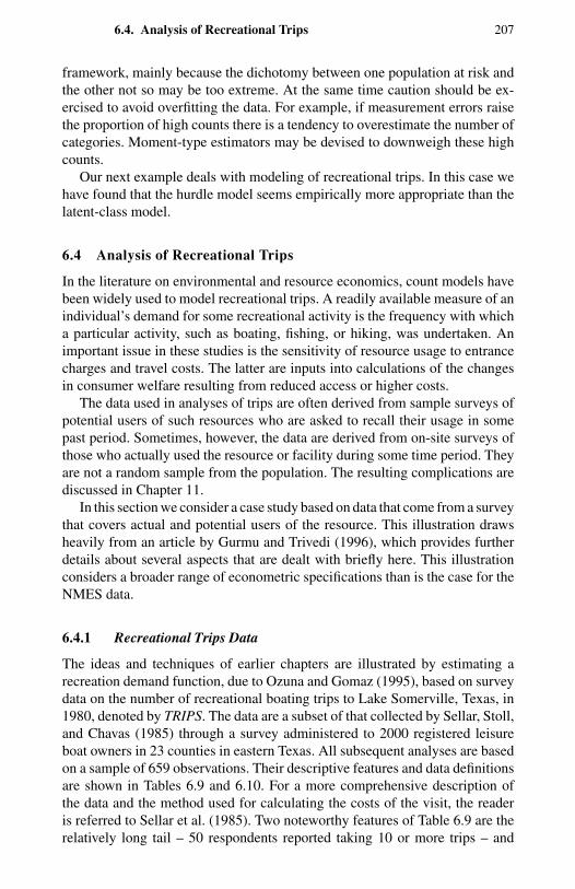
6.4. Analysis of Recreational Trips 207

framework, mainly because the dichotomy between one population at risk andthe other not so may be too extreme. At the same time caution should be ex-ercised to avoid overfitting the data. For example, if measurement errors raisethe proportion of high counts there is a tendency to overestimate the number ofcategories. Moment-type estimators may be devised to downweigh these highcounts.

Our next example deals with modeling of recreational trips. In this case wehave found that the hurdle model seems empirically more appropriate than thelatent-class model.

6.4 Analysis of Recreational Trips

In the literature on environmental and resource economics, count models havebeen widely used to model recreational trips. A readily available measure of anindividual’s demand for some recreational activity is the frequency with whicha particular activity, such as boating, fishing, or hiking, was undertaken. Animportant issue in these studies is the sensitivity of resource usage to entrancecharges and travel costs. The latter are inputs into calculations of the changesin consumer welfare resulting from reduced access or higher costs.

The data used in analyses of trips are often derived from sample surveys ofpotential users of such resources who are asked to recall their usage in somepast period. Sometimes, however, the data are derived from on-site surveys ofthose who actually used the resource or facility during some time period. Theyare not a random sample from the population. The resulting complications arediscussed in Chapter 11.

In this section we consider a case study based on data that come from a surveythat covers actual and potential users of the resource. This illustration drawsheavily from an article by Gurmu and Trivedi (1996), which provides furtherdetails about several aspects that are dealt with briefly here. This illustrationconsiders a broader range of econometric specifications than is the case for theNMES data.

6.4.1 Recreational Trips Data

The ideas and techniques of earlier chapters are illustrated by estimating arecreation demand function, due to Ozuna and Gomaz (1995), based on surveydata on the number of recreational boating trips to Lake Somerville, Texas, in1980, denoted by TRIPS. The data are a subset of that collected by Sellar, Stoll,and Chavas (1985) through a survey administered to 2000 registered leisureboat owners in 23 counties in eastern Texas. All subsequent analyses are basedon a sample of 659 observations. Their descriptive features and data definitionsare shown in Tables 6.9 and 6.10. For a more comprehensive description ofthe data and the method used for calculating the costs of the visit, the readeris referred to Sellar et al. (1985). Two noteworthy features of Table 6.9 are therelatively long tail – 50 respondents reported taking 10 or more trips – and

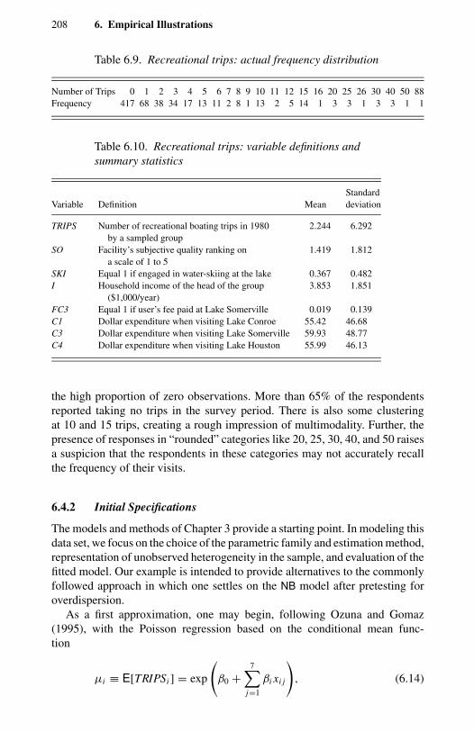
208 6. Empirical Illustrations

Table 6.9. Recreational trips: actual frequency distribution

Number of Trips 0 1 2 3 4 5 6 7 8 9 10 11 12 15 16 20 25 26 30 40 50 88Frequency 417 68 38 34 17 13 11 2 8 1 13 2 5 14 1 3 3 1 3 3 1 1

Table 6.10. Recreational trips: variable definitions andsummary statistics

StandardVariable Definition Mean deviation

TRIPS Number of recreational boating trips in 1980 2.244 6.292by a sampled group

SO Facility’s subjective quality ranking on 1.419 1.812a scale of 1 to 5

SKI Equal 1 if engaged in water-skiing at the lake 0.367 0.482I Household income of the head of the group 3.853 1.851

($1,000/year)FC3 Equal 1 if user’s fee paid at Lake Somerville 0.019 0.139C1 Dollar expenditure when visiting Lake Conroe 55.42 46.68C3 Dollar expenditure when visiting Lake Somerville 59.93 48.77C4 Dollar expenditure when visiting Lake Houston 55.99 46.13

the high proportion of zero observations. More than 65% of the respondentsreported taking no trips in the survey period. There is also some clusteringat 10 and 15 trips, creating a rough impression of multimodality. Further, thepresence of responses in “rounded” categories like 20, 25, 30, 40, and 50 raisesa suspicion that the respondents in these categories may not accurately recallthe frequency of their visits.

6.4.2 Initial Specifications

The models and methods of Chapter 3 provide a starting point. In modeling thisdata set, we focus on the choice of the parametric family and estimation method,representation of unobserved heterogeneity in the sample, and evaluation of thefitted model. Our example is intended to provide alternatives to the commonlyfollowed approach in which one settles on the NB model after pretesting foroverdispersion.

As a first approximation, one may begin, following Ozuna and Gomaz(1995), with the Poisson regression based on the conditional mean func-tion

µi ≡ E[TRIPSi ] = exp

(β0 +

7∑j=1

βi xi j

), (6.14)

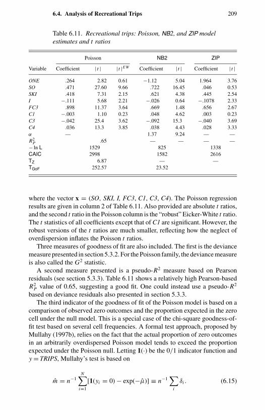
6.4. Analysis of Recreational Trips 209

Table 6.11. Recreational trips: Poisson, NB2, and ZIP modelestimates and t ratios

Poisson NB2 ZIP

Variable Coefficient | t | | t |EW Coefficient | t | Coefficient | t |

ONE .264 2.82 0.61 −1.12 5.04 1.964 3.76SO .471 27.60 9.66 .722 16.45 .046 0.53SKI .418 7.31 2.15 .621 4.38 .445 2.54I −.111 5.68 2.21 −.026 0.64 −.1078 2.33FC3 .898 11.37 3.64 .669 1.48 .656 2.67C1 −.003 1.10 0.23 .048 4.62 .003 0.23C3 −.042 25.4 3.62 −.092 15.3 −.040 3.69C4 .036 13.3 3.85 .038 4.43 .028 3.33α — 1.37 9.24 — —R2

P .65 — — — —− ln L 1529 825 1338CAIC 2998 1582 2616TZ 6.87 — —TGoF 252.57 23.52

where the vector x = (SO, SKI, I, FC3, C1, C3, C4). The Poisson regressionresults are given in column 2 of Table 6.11. Also provided are absolute t ratios,and the second t ratio in the Poisson column is the “robust” Eicker-White t ratio.The t statistics of all coefficients except that of C1 are significant. However, therobust versions of the t ratios are much smaller, reflecting how the neglect ofoverdispersion inflates the Poisson t ratios.

Three measures of goodness of fit are also included. The first is the deviancemeasure presented in section 5.3.2. For the Poisson family, the deviance measureis also called the G2 statistic.

A second measure presented is a pseudo-R2 measure based on Pearsonresiduals (see section 5.3.3). Table 6.11 shows a relatively high Pearson-basedR2

P value of 0.65, suggesting a good fit. One could instead use a pseudo-R2

based on deviance residuals also presented in section 5.3.3.The third indicator of the goodness of fit of the Poisson model is based on a

comparison of observed zero outcomes and the proportion expected in the zerocell under the null model. This is a special case of the chi-square goodness-of-fit test based on several cell frequencies. A formal test approach, proposed byMullahy (1997b), relies on the fact that the actual proportion of zero outcomesin an arbitrarily overdispersed Poisson model tends to exceed the proportionexpected under the Poisson null. Letting 1(·) be the 0/1 indicator function andy = TRIPS, Mullahy’s test is based on

m = n−1N∑

i=1

[1(yi = 0) − exp(−µ)] ≡ n−1∑

i

δi . (6.15)

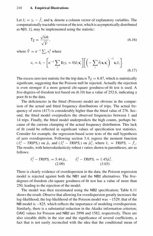
210 6. Empirical Illustrations

Let εi = yi − f i and xi denote a column vector of explanatory variables. Thecomputationally tractable version of the test, which is asymptotically distributedas N[0, 1], may be implemented using the statistic:

TZ =√

nm√V

, (6.16)

where V = n−1∑i v2

i where

vi = δi −[

n−1∑

i

1(yi = 0)εi x′i

][(−∑

i

θi xi x′i

)−1

xi εi

].

(6.17)

The excess zero test statistic for the trip data is TZ = 6.87, which is statisticallysignificant, suggesting that the Poisson null be rejected. Actually the rejectionis even stronger if a more general chi-square goodness-of-fit test is used. Afive-degrees-of-freedom test based on (6.10) has a value of 252.6, indicating apoor fit to the data.

The deficiencies in the fitted (Poisson) model are obvious in the compar-ison of the actual and fitted frequency distributions of trips. The actual fre-quency of zeros (417) is considerably higher than the fitted value of 276. Sec-ond, the fitted model overpredicts the observed frequencies between 1 and14 trips. Finally, the fitted model underpredicts the high counts, perhaps be-cause of the curious clumping of the actual frequency distribution. This lackof fit could be reflected in significant values of specification test statistics.Consider for example, the regression-based score tests of the null hypothesisof zero overdispersion. Following section 3.4, regress the moment function( ε2

i − TRIPSi ) on µi and ( ε2i − TRIPSi ) on µ2

i , where εi = TRIPSi − f i .The results, with heteroskedasticity robust t ratios shown in parentheses, are asfollows:

ε2i − TRIPSi = 5.44 µi ,

(2.09)ε2

i − TRIPSi = 1.45µ2i .

(3.03)

There is clearly evidence of overdispersion in the data; the Poisson regressionmodel is rejected against both the NB1 and the NB2 alternatives. The five-degrees-of-freedom chi-square goodness-of-fit test has a value of more than250, leading to the rejection of the model.

The model was then reestimated using the NB2 specification; Table 6.11shows the result. Observe that allowing for overdispersion greatly increases thelog-likelihood; the log-likelihood of the Poisson model was −1529; that of theNB model is −825, which reflects the importance of modeling overdispersion.Similarly, there is a substantial reduction in the Akaike information criterion;CAIC values for Poisson and NB2 are 2998 and 1582, respectively. There arealso sizeable shifts in the size and the significance of several coefficients, afact that is not easily reconciled with the idea that the conditional mean of

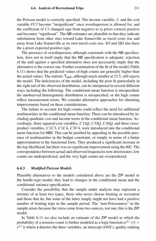
6.4. Analysis of Recreational Trips 211

the Poisson model is correctly specified. The income variable, I , and the costvariable FC3 become “insignificant” once overdispersion is allowed for, andthe coefficient of C1 changed sign from negative to (a priori correct) positiveand becomes “significant”. The NB estimates are plausible in that they indicatesubstitution from other sites toward Lake Somerville as travel costs rise andaway from Lake Somerville as its own travel costs rise. SO and SKI also havethe a priori expected positive sign.

The presence of overdispersion, although consistent with the NB specifica-tion, does not in itself imply that the NB specification is adequate; rejectionof the null against a specified alternative does not necessarily imply that thealternative is the correct one. Further examination of the fit of the model (Table6.11) shows that the predicted values of high counts are generally higher thanthe actual values. The statistic TGoF, although much smaller at 23.5, still rejectsthe model. The deficiencies of the model, including the poor fit particularly inthe right tail of the observed distribution, can be interpreted in several differentways including the following: The conditional mean function is misspecified;the unobserved heterogeneity distribution is misspecified; or the high countsreflect measurement errors. We consider alternative approaches for obtainingimprovements based on these considerations.

The failure to account for high counts could reflect the need for additionalnonlinearities in the conditional mean function. These can be introduced by in-cluding quadratic cost and income terms in the conditional mean function. Ac-cordingly, three squared-cost variables, C1SQ, C3SQ, C4SQ, and three cross-product variables, C1C3, C1C4, C3C4, were introduced into the conditionalmean function for NB2. This can be justified by appealing to the possible pres-ence of nonlinearities in the budget constraint, or simply in terms of a betterapproximation to the functional form. They produced a significant increase inthe log-likelihood, but there was no significant improvement using the AIC. Thecorrespondence between actual and observed frequencies now deteriorates; lowcounts are underpredicted, and the very high counts are overpredicted.

6.4.3 Modified Poisson Models

Plausible alternatives to the models considered above are the ZIP model orthe hurdle-type model; they lead to changes in the conditional mean and theconditional variance specification.

Consider the possibility that the sample under analysis may represent amixture of at least two types, those who never choose boating as recreationand those that do, but some of the latter simply might not have had a positivenumber of boating trips in the sample period. The “non-Poissonness” in thesample arises because the zeros come from two sources, not one; this is the ZIPmodel.

In Table 6.11 we also include an estimate of the ZIP model in which theprobability of a nonzero count is further modeled as a logit function (ez′γ /(1 +ez′γ )) where z denotes the three variables, an intercept (ONE ), quality ranking

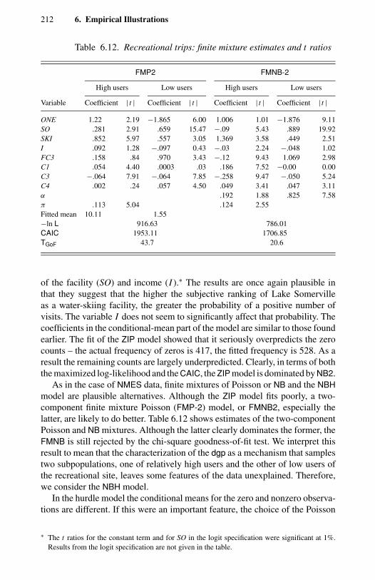
212 6. Empirical Illustrations

Table 6.12. Recreational trips: finite mixture estimates and t ratios

FMP2 FMNB-2

High users Low users High users Low users

Variable Coefficient | t | Coefficient | t | Coefficient | t | Coefficient | t |

ONE 1.22 2.19 −1.865 6.00 1.006 1.01 −1.876 9.11SO .281 2.91 .659 15.47 −.09 5.43 .889 19.92SKI .852 5.97 .557 3.05 1.369 3.58 .449 2.51I .092 1.28 −.097 0.43 −.03 2.24 −.048 1.02FC3 .158 .84 .970 3.43 −.12 9.43 1.069 2.98C1 .054 4.40 .0003 .03 .186 7.52 −0.00 0.00C3 −.064 7.91 −.064 7.85 −.258 9.47 −.050 5.24C4 .002 .24 .057 4.50 .049 3.41 .047 3.11α .192 1.88 .825 7.58π .113 5.04 .124 2.55Fitted mean 10.11 1.55−ln L 916.63 786.01CAIC 1953.11 1706.85TGoF 43.7 20.6

of the facility (SO) and income (I ).∗ The results are once again plausible inthat they suggest that the higher the subjective ranking of Lake Somervilleas a water-skiing facility, the greater the probability of a positive number ofvisits. The variable I does not seem to significantly affect that probability. Thecoefficients in the conditional-mean part of the model are similar to those foundearlier. The fit of the ZIP model showed that it seriously overpredicts the zerocounts – the actual frequency of zeros is 417, the fitted frequency is 528. As aresult the remaining counts are largely underpredicted. Clearly, in terms of boththe maximized log-likelihood and the CAIC, the ZIP model is dominated by NB2.

As in the case of NMES data, finite mixtures of Poisson or NB and the NBHmodel are plausible alternatives. Although the ZIP model fits poorly, a two-component finite mixture Poisson (FMP-2) model, or FMNB2, especially thelatter, are likely to do better. Table 6.12 shows estimates of the two-componentPoisson and NB mixtures. Although the latter clearly dominates the former, theFMNB is still rejected by the chi-square goodness-of-fit test. We interpret thisresult to mean that the characterization of the dgp as a mechanism that samplestwo subpopulations, one of relatively high users and the other of low users ofthe recreational site, leaves some features of the data unexplained. Therefore,we consider the NBH model.

In the hurdle model the conditional means for the zero and nonzero observa-tions are different. If this were an important feature, the choice of the Poisson

∗ The t ratios for the constant term and for SO in the logit specification were significant at 1%.Results from the logit specification are not given in the table.

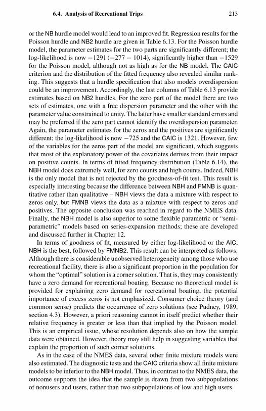
6.4. Analysis of Recreational Trips 213

or the NB hurdle model would lead to an improved fit. Regression results for thePoisson hurdle and NB2 hurdle are given in Table 6.13. For the Poisson hurdlemodel, the parameter estimates for the two parts are significantly different; thelog-likelihood is now −1291 (−277 − 1014), significantly higher than −1529for the Poisson model, although not as high as for the NB model. The CAICcriterion and the distribution of the fitted frequency also revealed similar rank-ing. This suggests that a hurdle specification that also models overdispersioncould be an improvement. Accordingly, the last columns of Table 6.13 provideestimates based on NB2 hurdles. For the zero part of the model there are twosets of estimates, one with a free dispersion parameter and the other with theparameter value constrained to unity. The latter have smaller standard errors andmay be preferred if the zero part cannot identify the overdispersion parameter.Again, the parameter estimates for the zeros and the positives are significantlydifferent; the log-likelihood is now −725 and the CAIC is 1321. However, fewof the variables for the zeros part of the model are significant, which suggeststhat most of the explanatory power of the covariates derives from their impacton positive counts. In terms of fitted frequency distribution (Table 6.14), theNBH model does extremely well, for zero counts and high counts. Indeed, NBHis the only model that is not rejected by the goodness-of-fit test. This result isespecially interesting because the difference between NBH and FMNB is quan-titative rather than qualitative – NBH views the data a mixture with respect tozeros only, but FMNB views the data as a mixture with respect to zeros andpositives. The opposite conclusion was reached in regard to the NMES data.Finally, the NBH model is also superior to some flexible parametric or “semi-parametric” models based on series-expansion methods; these are developedand discussed further in Chapter 12.

In terms of goodness of fit, measured by either log-likelihood or the AIC,NBH is the best, followed by FMNB2. This result can be interpreted as follows:Although there is considerable unobserved heterogeneity among those who userecreational facility, there is also a significant proportion in the population forwhom the “optimal” solution is a corner solution. That is, they may consistentlyhave a zero demand for recreational boating. Because no theoretical model isprovided for explaining zero demand for recreational boating, the potentialimportance of excess zeros is not emphasized. Consumer choice theory (andcommon sense) predicts the occurrence of zero solutions (see Pudney, 1989,section 4.3). However, a priori reasoning cannot in itself predict whether theirrelative frequency is greater or less than that implied by the Poisson model.This is an empirical issue, whose resolution depends also on how the sampledata were obtained. However, theory may still help in suggesting variables thatexplain the proportion of such corner solutions.

As in the case of the NMES data, several other finite mixture models werealso estimated. The diagnostic tests and the CAIC criteria show all finite mixturemodels to be inferior to the NBH model. Thus, in contrast to the NMES data, theoutcome supports the idea that the sample is drawn from two subpopulationsof nonusers and users, rather than two subpopulations of low and high users.

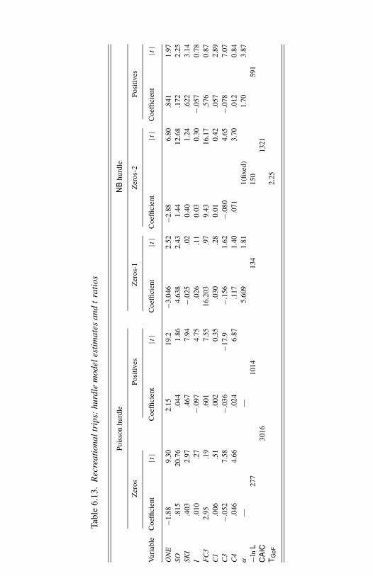
Tabl

e6.

13.

Rec

reat

iona

ltri

ps:

hurd

lem

odel

esti

mat

esan

dt

rati

os

Pois

son

hurd

leN

Bhu

rdle

Zer

osPo

sitiv

esZ

eros

-1Z

eros

-2Po

sitiv

es

Var

iabl

eC

oeffi

cien

t|t

|C

oeffi

cien

t|t

|C

oeffi

cien

t|t

|C

oeffi

cien

t|t

|C

oeffi

cien

t|t

|

ON

E−1

.88

9.30

2.15

19.2

−3.0

462.

52−2

.88

6.80

.841

1.97

SO.8

1520

.76

.044

1.86

4.63

82.

431.

4412

.68

.172

2.25

SKI

.403

2.97

.467

7.94

−.02

5.0

20.

401.

24.6

223.

14I

.010

.27

−.09

74.

75.0

26.1

10.

030.

30−.

057

0.78

FC

32.

95.1

9.6

017.

5516

.203

.97

9.43

16.1

7.5

760.

87C

1.0

06.5

1.0

020.

35.0

30.2

80.

010.

42.0

572.

89C

3−.

052

7.58

−.03

6−1

7.9

−.15

61.

62−.

080

4.65

−.07

87.

07C

4.0

464.

66.0

246.

87.1

171.

40.0

713.

70.0

120.

84α

——

5.60

91.

811(

fixed

)1.

703.

87−l

nL

277

1014

134

150

591

CA

IC30

1613

21T

GoF

2.25

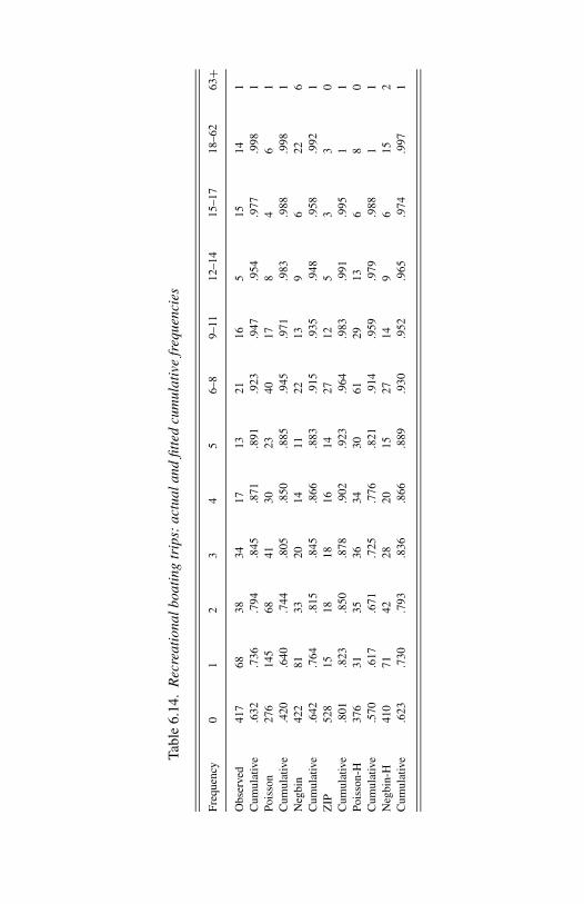
Tabl

e6.

14.

Rec

reat

iona

lboa

ting

trip

s:ac

tual

and

fitte

dcu

mul

ativ

efr

eque

ncie

s

Freq

uenc

y0

12

34

56–

89–

1112

–14

15–1

718

–62

63+

Obs

erve

d41

768

3834

1713

2116

515

141

Cum

ulat

ive

.632

.736

.794

.845

.871

.891

.923

.947

.954

.977

.998

1Po

isso

n27

614

568

4130

2340

178

46

1C

umul

ativ

e.4

20.6

40.7

44.8

05.8

50.8

85.9

45.9

71.9

83.9

88.9

981

Neg

bin

422

8133

2014

1122

139

622

6C

umul

ativ

e.6

42.7

64.8

15.8

45.8

66.8

83.9

15.9

35.9

48.9

58.9

921

ZIP

528

1518

1816

1427

125

33

0C

umul

ativ

e.8

01.8

23.8

50.8

78.9

02.9

23.9

64.9

83.9

91.9

951

1Po

isso

n-H

376

3135

3634

3061

2913

68

0C

umul

ativ

e.5

70.6

17.6

71.7

25.7

76.8

21.9

14.9

59.9

79.9

881

1N

egbi

n-H

410

7142

2820

1527

149

615

2C

umul

ativ

e.6

23.7

30.7

93.8

36.8

66.8

89.9

30.9

52.9

65.9

74.9

971

216 6. Empirical Illustrations

6.4.4 Economic Implications

The model discrimination and selection exercise rely heavily on statistical crite-ria in both applications. Are we simply fine-tuning the model, or are the resultingchanges economically meaningful? Only a partial answer can be given here. Inthe modeling of recreational trips it is reasonable to suppose that a random sam-ple includes nonparticipants because of taste differences among individuals. Ahurdles-type model is worthwhile in this case because parameter estimates andwelfare analysis should be based only on the participant’s responses. In thecase of NMES data on the elderly, the notion of nonparticipants is implausible.However, given differences in health status of individuals as well as other typesof unobserved heterogeneity, the distinction between high users and low usersis reasonable. This feature can explain the superior performance of the finitemixture NB model.

6.5 LR Test: A Digression

The two examples in this chapter illustrate alternative ways of handling “non-Poisson” features of two data sets. The hurdles version provides a good fit to therecreational trips data, and the latent-class approach a good fit to the doctor visitsdata. These outcomes can also be rationalized in terms of a priori reasoning.Distinguishing between hurdles and finite-mixture models may be difficult inmany situations, in which neither formulation may be a priori unacceptable.Furthermore, one might also construct finite mixtures based on hurdles, whichwould involve finite mixtures of binomials for the zero outcome, and finitemixtures of truncated counts for the positives. Identification and estimation ofsuch models is likely to prove challenging.

6.5.1 Simulation Analysis of Model Selection Criteria

This section reports the results of a small simulation experiment designed tothrow light on the properties of model evaluation criteria used in this chapter.

Simulation Design

Data were generated using, respectively, the Poisson, Poisson hurdles, andFMP2 structures. The conditional mean in each case was specified thus:

Poisson: µi = exp [−1.445 + 3.0xi ]PH: Zeros part: µi = exp [−1.6 + 3.0xi ];

positives: µi = exp [−1.35 + 3.0xi ]FMP2: µ1 = exp [−1.225 + 3.0xi ]; µ2 = exp [−1.5 + .75xi ];

π = 0.75

The dgp was calibrated in each case to mimic the excess zeros situation. Thezeros accounted for about 40% of the observations. We examine the frequency

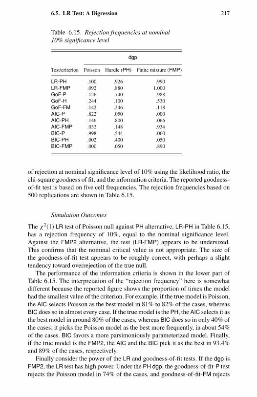
6.5. LR Test: A Digression 217

Table 6.15. Rejection frequencies at nominal10% significance level

dgp

Test/criterion Poisson Hurdle (PH) Finite mixture (FMP)

LR-PH .100 .926 .990LR-FMP .092 .880 1.000GoF-P .126 .740 .988GoF-H .244 .100 .530GoF-FM .142 .346 .118AIC-P .822 .050 .000AIC-PH .146 .800 .066AIC-FMP .032 .148 .934BIC-P .998 .544 .060BIC-PH .002 .400 .050BIC-FMP .000 .050 .890

of rejection at nominal significance level of 10% using the likelihood ratio, thechi-square goodness of fit, and the information criteria. The reported goodness-of-fit test is based on five cell frequencies. The rejection frequencies based on500 replications are shown in Table 6.15.

Simulation Outcomes

The χ2(1) LR test of Poisson null against PH alternative, LR-PH in Table 6.15,has a rejection frequency of 10%, equal to the nominal significance level.Against the FMP2 alternative, the test (LR-FMP) appears to be undersized.This confirms that the nominal critical value is not appropriate. The size ofthe goodness-of-fit test appears to be roughly correct, with perhaps a slighttendency toward overrejection of the true null.

The performance of the information criteria is shown in the lower part ofTable 6.15. The interpretation of the “rejection frequency” here is somewhatdifferent because the reported figure shows the proportion of times the modelhad the smallest value of the criterion. For example, if the true model is Poisson,the AIC selects Poisson as the best model in 81% to 82% of the cases, whereasBIC does so in almost every case. If the true model is the PH, the AIC selects it asthe best model in around 80% of the cases, whereas BIC does so in only 40% ofthe cases; it picks the Poisson model as the best more frequently, in about 54%of the cases. BIC favors a more parsimoniously parameterized model. Finally,if the true model is the FMP2, the AIC and the BIC pick it as the best in 93.4%and 89% of the cases, respectively.

Finally consider the power of the LR and goodness-of-fit tests. If the dgp isFMP2, the LR test has high power. Under the PH dgp, the goodness-of-fit-P testrejects the Poisson model in 74% of the cases, and goodness-of-fit-FM rejects

218 6. Empirical Illustrations

the FMP model in only 34.6% of the cases. In the converse case in which the dgpis the FMP model, the goodness-of-fit-P test rejects the Poisson in 98.8% of thecases, and goodness-of-fit-H rejects the hurdle model in only 53.3% of the cases.Of course, these results are affected by the choice of parameter values. However,these results indicate that the discrimination between the hurdles and the finitemixture models using the goodness-of-fit test may be more difficult than thediscrimination between the one-component model and a mixture alternative.

To summarize, collectively, the goodness-of-fit tests and the information cri-teria are useful in evaluating models. Rejection of the null by the LR, goodness-of-fit, or the AIC would seem to indicate a deficiency of the model. Thus,despite its theoretical limitations, the standard LR test of the one-componentmodel against the mixture alternative may have useful power.

6.5.2 Bootstrapping the LR Test

If computational cost is not an important consideration, a parametric bootstrapof the LR test provides another way to obtain better critical values for the test.Feng and McCulloch (1996) suggested and analyzed a bootstrap LR test forthe null that the number of components in the mixture is C − 1 against thealternative that it is C. Their examples are in a univariate iid setting. Hencetheir procedure must be adapted to the non-iid regression case, as discussed insection 5.5. As an illustration we consider the case C = 2.

1. Estimate the one-component model and the two-component mixturemodel by MLE. Form the LR statistic, denoted LR∗.

2. Draw a bootstrap pseudosample (y∗i , x∗

i ) by sampling with replace-ment from the original sample (yi , xi ), i = 1, . . . , n. Estimate the nullmodel and construct the LR statistic.

3. Repeat steps 1 and 2 B times, giving B values of the LR statistic,denoted L Ri , i = 1, . . . , B.

4. Using the bootstrap distribution of the LR statistic, determine the(1 − α) percent quantile as the critical value, denoted LRB .

5. Reject H0 if LR∗ > LRB .

The procedure generalizes to other null and alternative models. Applicationof this procedure to the NMES sample would have been prohibitively expensiveif we had set B = 100 or more.

6.6 Concluding Remarks

Most empirical studies generate substantive and methodological questions thatmotivate subsequent investigations. We conclude by mentioning two issues andlines of investigation worth pursuing. First, in the context of the recreationaltrips example, one might question the assumption of independence of sampleobservations. This is standard in cross-section analysis. However, our data also

6.7. Bibliographic Notes 219

have a spatial dimension. Even after conditioning, observations may be spatiallycorrelated. This feature will affect the estimated variances of the parameters.Essentially, the assumption of independent observations implies that our sampleis more informative than might actually be the case.

A related issue concerns the stochastic process for events. Many events maybelong to a spell of events, and each spell may constitute several correlatedevents. The spells themselves may follow some stochastic process and may infact be observable. One might then consider whether to analyze pooled dataor to analyze events grouped by spells. An example is the number of doctorvisits within a spell of illness (Newhouse, 1993). In many data situations one isuncertain whether the observed events are a part of the same spell or differentspells.

Another issue is joint modeling of several types of events. The empiricalexamples considered in this chapter involve conditional models for individualevents, not joint models for several events. This may be restrictive. In somestudies the event of interest generates multiple observations on several counts.A health event, for instance, may lead to hospitalization, doctor consultations,and usage of prescribed medicines, all three being interrelated. The analysisdescribed in the previous paragraph can be extended to this type of situationby considering a mixture of multinomial and count models, which leads tomultivariate count models, a topic that is discussed in Chapter 8.

6.7 Bibliographic Notes

Applications of single-equation count data models in economics, especially inaccident analysis, insurance, health, labor, and resource and environmental eco-nomics, are now standard; examples are Johansson and Palme (1996), Pohlmeierand Ulrich (1995), Gurmu and Trivedi (1996), and Grogger and Carson (1991).Rose (1990) uses Poisson models to evaluate the effect of regulation on airlinesafety record. Dionne and Vanasse (1992) use a sample of about 19,000 Quebecdrivers to estimate an NB2 model that is used to derive predicted claims fre-quencies, and hence insurance premia, from data on different individuals withdifferent characteristics and records. Schwartz and Torous (1993) combine thePoisson regression approach with the proportional hazard structure. They sepa-rately model monthly grouped data on mortgage prepayments and defaults, thetwo being modeled separately. Lambert (1992) provides an interesting anal-ysis of the number of defects in a manufacturing process using the Poissonregression with “excess zeros.” Cameron and Trivedi (1996) survey this and anumber of other count data applications in financial economics. Nagin and Land(1993) use the Heckman-Singer–type nonparametric approach in their mixedPoisson longitudinal data model of criminal careers. Their model is essentiallya hurdles-type Poisson model with nonparametric treatment of heterogeneity.After estimation, they classify observations into groups according to criminalpropensity, in a manner analogous to that used in the health utilization exam-ple. Cameron and Windmeijer (1996) consider pseudo-R2–type goodness-of-fit

220 6. Empirical Illustrations

measures for Poisson and NB models. Panel data applications are featured inChapter 9. Two interesting marketing applications of latent class (finite mixture)count models are Wedel et al. (1993) and Ramaswamy, Anderson, and DeSarbo(1994). Wang, Cockburn, and Puterman (1998) apply the finite mixture modelto patent data; they also parameterize the sampling fractions as functions of co-variates. Haab and McConnell (1996) discuss estimation of consumer surplusmeasures in the presence of excess zeros.

6.8 Exercises

6.1 Using the estimated mixing proportion π1 in Table 6.6, and the estimatedcomponent means in Table 6.7, check whether the sample mean of OFP givenin Table 6.2 coincides with the fitted mean. Using the first-order conditions formaximum likelihood estimation of NB2, consider whether a two-componentfinite mixture of the NB2 model will display an analogous property.

6.2 Suppose the dgp is a two-component CFMNB family, with the slope pa-rameters of the conditional mean functions equal but intercepts left free. Aninvestigator misspecifies the model and estimates a unicomponent Poisson re-gression model instead. Show that the Poisson MLE consistently estimates theslope parameters.

6.3 In the context of the modeling the zeros/positives binary outcome using theNBH specification, compare the following two alternatives from the viewpointof identifiability of the parameters (β,α1),

Pr [yi = 0 | xi ] =1/(1 + α1µi )1/α1 , or

1/(1 + µi ),

where µi = exp(x′iβ).

6.4 Consider how to specify and estimate a two-component finite mixture ofthe NBH model. Show that this involves a mixture of binomials as well as amixture of NB families.

6.5 Consider whether the alternative definitions of residuals in Chapter 5 canbe extended to finite mixtures of Poisson components.

6.6 Verify the result given in (6.12). To do so, first derive (4.62) for r = 2,then derive the central second moment by subtracting off µ2.

CHAPTER 7

Time Series Data

7.1 Introduction

The previous chapters have focused on models for cross-section regression on asingle count dependent variable. We now turn to models for more general typesof data – univariate time series data in this chapter, multivariate cross-sectiondata in Chapter 8, and longitudinal or panel data in Chapter 9.

Count data introduce complications of discreteness and heteroskedasticity.For cross-section data, this leads to moving from the linear model to the Poissonregression model. This model is often too restrictive for real data, which aretypically overdispersed. With cross-section data, overdispersion is most fre-quently handled by leaving the conditional mean unchanged and rescaling theconditional variance. The same adjustment is made regardless of whether theunderlying cause of overdispersion is unobserved heterogeneity in a Poissonpoint process or true contagion leading to dependence in the process.

For time series count data, one can again begin with the Poisson regressionmodel. In this case, however, it is not clear how to proceed if dependence ispresent. For example, developing even a pure time series count model in whichthe count in period t , yt , depends only on the count in the previous period,yt−1, is not straightforward, and there are many possible ways to proceed. Evenrestricting attention to a fully parametric approach, one can specify distributionsfor yt either conditional on yt−1 or unconditional on yt−1. For count data thisleads to quite different models, whereas for continuous data the assumption ofjoint normality leads to both conditional and marginal distributions that are alsonormal.

Time series models for count data are in their infancy, yet remarkably manymodels have been developed. These models, although conceptually and in somecases mathematically innovative, are generally restrictive. For example, somemodels restrict serial correlation to being positive. At this stage it is not clearwhich, if any, of the current models will become the dominant model for timeseries count data.

A review of linear time series models is given in section 7.2, along with abrief summary of six different classes of count time series models. In section 7.3

222 7. Time Series Data

we consider estimation of static regression models and residual-based tests forserial correlation. In sections 7.4 through 7.9 each of the six models is presentedin detail. In section 7.10 some of these models are applied to monthly time seriesdata on the number of contract strikes in U.S. manufacturing, first introducedin section 7.3.4.

Estimators for basic static and dynamic regression models, controlling forboth autocorrelation and heteroskedasticity present in time series data, are de-tailed in sections 7.3 to 7.6. The simplest, although not necessarily fully effi-cient, estimators for these models are relatively straightforward to implement.For many applied studies this is sufficient. For a more detailed analysis of data,the models of sections 7.4, 7.7, and 7.8 are particularly appealing. Estimation(efficient estimation in the case of section 7.4) of these models entails complexmethods. Implementation requires reading the original papers.

7.2 Models for Time Series Data

7.2.1 Linear Models

For a continuous dependent variable, the standard models are well established.For pure time series, where the only explanatory variables are lagged values ofthe dependent variable, the standard class of linear models is the autoregres-sive moving average model of orders p and q , or ARMA(p, q), model. In theARMA(p, q) model, the current value of y is the weighted sum of the past pvalues of y and the current and past q values of an iid error

yt = ρ1 yt−1 + · · · + ρp yt−p + εt + γ1εt−1 + · · · + γqεt−q ,

t = p + 1, . . . , T, (7.1)

where εt is iid (0, σ 2).For linear time series regression the explanatory variables include exogenous

regressors. The autoregressive or dynamic model includes exogenous regressorsand lagged dependent variables in the regression function. An example is

yt = ρyt−1 + x′tβ + εt , (7.2)

where the error term εt is iid (0, σ 2). Note that this model is equivalent toassuming that

yt | yt−1 ∼ D[ρyt−1 + x′

tβ, σ 2], (7.3)

that is, yt conditional on yt−1 and xt is distributed with mean ρyt−1 + x′tβ and

variance σ 2. More generally, additional lags of y and x may appear as regressors.If only xt and lags of xt appear, the model is instead called a distributed lagmodel. If xt alone appears as a regressor, the model is called a static model.

7.2. Models for Time Series Data 223

An alternative time series regression model is the serially correlated errormodel. This starts with a static regression function

yt = x′tβ + ut , (7.4)

but then assumes that the error term ut is serially correlated, following forexample an ARMA process. The simplest case is an autoregressive error oforder one (AR[1]) error

ut = ρut−1 + εt , (7.5)

where εt is iid (0, σ 2). Then the model can be rewritten as

yt = ρyt−1 + x′tβ − x′

t−1βρ + εt , (7.6)

which is an autoregressive model with nonlinear restrictions imposed on theparameters.

The autoregressive and serial correlation models can be combined, to yieldan autoregressive model with serially correlated error.

Estimation for these models is by NLS, or by maximum likelihood if a dis-tribution is specified for εt . For models with autoregressive errors of orderp, specification of a normal distribution for εt leads by change of variabletechniques to a joint density for yp+1, . . . , yT , given y1, . . . , yp, which is max-imized by the MLE. Alternatively, the NLS estimator minimizes the sum ofsquared residuals,

∑Tt=p+1 ε2

t . For example the model in (7.4) and (7.5) leads toεt defined implicitly in (7.6), which leads to first-order conditions that are non-linear in parameters. Because εt is homoskedastic and uncorrelated, inferencefor the NLS estimator is the same as in the non–time series case. Note that if ut isserially correlated, it is

∑t ε2

t rather than∑

t u2t that is minimized. Minimizing

the latter would lead to estimates that are inefficient and even inconsistent iflagged dependent variables appear as regressors. The MLE and NLS estimatorare asymptotically equivalent, although they differ in small samples due to dif-ferent treatment of the first observation y1. For models with a moving averagecomponent in the error, estimation is more complicated but covered in standardtime series texts.

Recent econometrics literature on linear models for continuous data has fo-cused on models with unit roots, where ρ in (7.2) or (7.5) takes the value ρ = 1,and the related analysis of cointegrated time series. Then yt is nonstationary,due to a nonstationary stochastic trend, and the usual asymptotic normal the-ory for estimators no longer applies. Nonstationary stochastic trends have notbeen studied for count regression. Nonstationarity is instead accommodated bydeterministic trends, in which case the usual asymptotic theory still applies.

The preceding models are only those most commonly used for continuousdata. There are many extensions, two of which are now presented and alsoconsidered subsequently in the count context.

The state-space or time-varying parameter model is a modification of (7.4)that introduces dependence through parameters that vary over time rather than

224 7. Time Series Data

through the error term. An example is

yt = x′tβt + εt

βt −β = Φ(βt−1 −β) + υt ,(7.7)

where εt is iid (0, σ 2), Φ is a k × k matrix, and υt is a k × 1 iid (0,Σ) errorvector. If the roots of Φ lie inside the unit circle this model is stationary. Themodel is estimated by reexpressing it in state space form and using the Kalmanfilter (Harvey, 1989). This model is also widely used in Bayesian analysis oftime series, where it is called the dynamic linear model. A detailed treatmentis given in West and Harrison (1997).

The hidden Markov model, or regime shift model, is an extension of thepreceding models that additionally allows the parameters to differ accordingto which of a finite number of regimes is currently in effect. The unobservedregimes evolve over time according to a Markov chain – hence the term hiddenMarkov models. These models were popularized in economics by Hamilton(1989), who considered a two-regime Markov trend model

y∗t = α1dt1 + α2dt2 + y∗

t−1, (7.8)

where y∗t is the trend component of yt , and dt j are indicator variables for whether

or not in regime j , j = 1 or 2. The transitions between the two regimes aredetermined by realization ct of the first-order Markov chain Ct with transitionprobabilities

γi j = Pr [Ct = j | Ct−1 = i] , i, j = 1, 2, (7.9)

where γ1i + γ2i = 1. Then

dt j =

1 if ct = j

0 otherwisej = 1, 2. (7.10)

Parameters to be estimated are the intercepts α1 and α2, the transition proba-bilities γ11 and γ21, and the parameters in the model for the trend componenty∗

t of the actual data yt . An even simpler example sets y∗t = yt and omits y∗

t−1from (7.8), in which case dynamics are introduced solely via the Markov chaindetermining the regime switches.

7.2.2 Count Models

There are many possible time series models for count data. Different modelsarise through different models of the dependency of yt on past y, current andpast x, and the latent process or error process εt ; through different models ofthe latent process; and through different extensions of basic models.

Before presenting the various count models in detail, it is helpful to providea summary. For simplicity the role of regressors other than lagged dependentvariables is suppressed.

7.2. Models for Time Series Data 225

1. Integer-valued ARMA (or INARMA) models specify yt to be the sumof an integer whose value is determined by past yt and an indepen-dent innovation. Appropriate distributional assumptions lead to a countmarginal distribution of yt such as Poisson or NB2. This is a general-ization of the autoregressive model (7.2).

2. Autoregressive models or Markov models specify the conditional dis-tribution of yt to be a count distribution such as Poisson or NB2, withmean parameter that is a function of lagged values of yt . This is an ex-tension of (7.3), and hence also the autoregressive model (7.2). Herethe conditional distribution of yt is specified, whereas the INARMAmodel specifies the marginal distribution of yt .

3. Serially correlated error models or latent variable models let yt dependon a static component and a serially correlated latent variable. This isan extension of the serially correlated error model in (7.4) and (7.5).

4. State-space models or time-varying parameter models specify the dis-tribution of yt to be a count distribution such as Poisson or NB2, withconditional mean or parameters of the conditional mean that depend ontheir values in previous periods. This is an extension of the state-spacemodel (7.7).

5. Hidden Markov models or regime shift models specify the distributionof yt to be a count distribution such as Poisson or NB2, with parametersthat vary according to which of a finite number of regimes is currentlyin effect. The unobserved regimes evolve over time according to aMarkov chain. This is an extension of (7.8) and (7.9).

6. Discrete ARMA (DARMA) models introduce time dependency througha mixture process.

Attempts have been made to separate these models into classes of models,but there is no simple classification system that nests all models. Some authorsfollow Cox (1981) and refer to models as either observation-driven, with timeseries dependence introduced by specifying conditional moments or densitiesas explicit functions of past outcomes, or parameter-driven, with dependenceinduced by a latent variable process.

Others distinguish between conditional models, where the moments or den-sity are conditional on both xt and past outcomes of yt , and marginal models,where conditioning is only on xt and not on past outcomes of yt . This is mostuseful for distinguishing between models 1 and 2.

Once a model is specified, maximum likelihood estimation is generally notas straightforward as in the normal case. NLS estimation is usually possible butmay be inefficient, as the error term may be heteroskedastic or autocorrelated.Estimation is often by nonlinear feasible GLS or by GMM.

Criteria for choosing among various models include ease of estimation –models 1 through 3 are best – and similarity to standard time series modelssuch as having a serial correlation structure similar to ARMA models – models1 and 6 are best. One should also consider the appropriateness of models to

226 7. Time Series Data

count data typically encountered and the problem at hand. If interest lies inthe role of regressor variables, a static model of E[yt | xt ] may be sufficient.For forecasting, a conditional model of E[yt | xt , yt−1, yt−2, . . .] may be moreuseful.

7.3 Static Regression

Before studying in detail various time series count models, we consider staticregression, such as Poisson regression of yt on xt , and some simple extensions.We present a method for valid statistical inference in the presence of serialcorrelation. Residual-based tests for serial correlation are also presented, withimplementation easiest if standardized residuals are used.

Sometimes a static regression may be sufficient. Several regression applica-tions of time series of counts, cited here, find little or no serial correlation. Thenthere is no need to use the models presented in this chapter. This may seemsurprising, but it should be recalled that a pure Poisson point process generatesa time series of independent counts.

7.3.1 Estimation

We consider estimation of a static regression model, with exponential condi-tional mean

E[yt | xt ] = exp(x′

tβ). (7.11)

Conditional on static regressors xt , the dependent variable yt may be hete-roskedastic, as is common for count data, and serially correlated, as is commonfor time series data. It is relatively easy to obtain a consistent estimator of β.Both NLS and the Poisson PMLE maintain their consistency in the presenceof autocorrelation, if (7.11) still holds. More difficult is obtaining a consistentestimator of the variance matrix of these estimators, which is necessary forstatistical inference. We assume that autocorrelation is present to lag l, anddefine

ωt j = E[(yt − µt )(yt− j − µt− j ) | x1, . . . , xT ], j = 0, . . . , l,(7.12)

where µt = exp(x′tβ).

The NLS estimator, βNLS, minimizes∑T

t=1(yt − exp(x′tβ))2. Applying to

(7.11) results in White and Domowitz (1984), who considered general regres-sion function g(xt ,β), βNLS is asymptotically normal with meanβ and variancematrix

V[βNLS ] =(

T∑t=1

µ2t xt x′

t

)−1

BNLS

(T∑

t=1

µ2t xt x′

t

)−1

, (7.13)

7.3. Static Regression 227

where

BNLS =T∑

t=1

ωt0µ2t xt x′

t +l∑

j=1

T∑t=l

ωt jµtµt− j(xt x′

t− j + xt− j x′t

).

(7.14)

Note that if there is no autocorrelation at all in yt , so ωt j = 0 for j = 0, thevariance matrix simplifies to that for the cross-section case given in section3.7.3.

A similar result holds if instead one uses the Poisson PMLE,βP, presentedin section 3.2.3. ThenβP is asymptotically normal with mean β and variancematrix

V[βP] =(

T∑t=1

µt xt x′t

)−1

BP

(T∑

t=1

µt xt x′t

)−1

, (7.15)

where

BP =T∑

t=1

ωt0xt x′t +

l∑j=1

T∑t=l

ωt j(xt x′

t− j + xt− j x′t

). (7.16)

See exercise 7.1 for a way to derive this result. It is expected but not guaranteedthat the Poisson PMLE will lead to more efficient estimates than NLS, becausethe Poisson PMLE uses a working matrix that allows for heteroskedasticity.

The robust sandwich estimate of these variance matrices replaces µt byµt = exp(x′

tβ) and ωt j by (yt − µt )(yt− j − µt− j ). Some models presentedbelow place more structure on variances and autocovariances, that is, on ωt j .In particular, we expect ωt j to be a function of µt and µt− j . Then consistentestimates ωt j of ωt j may be used in (7.14) or (7.16). In these cases it is better, ofcourse, to use estimators of β that use this knowledge of ωt j , as they generallyare more efficient than NLS or the Poisson PMLE.

The results (7.13) and (7.15) extend immediately to distributed lag models.Then interpret xt as including lagged exogenous variables as well as contempo-raneous exogenous variables. The results also extend to dynamic models withlagged dependent variables as regressors, provided enough lags are included toensure that there is no serial correlation in yt after controlling for regressors, soωt j = 0 for j = 0.

The results do not apply if lagged dependent variables are regressors andthere is serial correlation in yt after controlling for regressors. Then the NLSand Poisson PML estimators are inconsistent, just as the OLS estimator is in-consistent in similar circumstances in the linear model.

7.3.2 Tests of Serial Correlation

Serial correlation tests are useful for several reasons. Tests based on residualsfrom static regressions can indicate if any time series corrections are necessary,

228 7. Time Series Data

or if instead results from the previous chapters can still be used. Tests basedon residuals from dynamic regressions can indicate whether, after inclusion oflagged variables, there is still autocorrelation that needs to be controlled for.

Let zt denote a detrended zero mean time series such as the deviation of theoriginal dependent count from the sample mean, zt = yt − y, or the residualfrom a regression model such as Poisson, zt = yt − µt . The standard measureof time series correlation is the autocorrelation at lag k,

ρk = E[zt zt−k]√E[z2

t

]E[z2

t−k

] . (7.17)

Raw residuals from Poisson regression are nonstationary, with nonconstantvariance because the variance equals the mean, which is nonconstant. Thus theraw residuals from count regression need to be standardized before performingthe standard tests of serial correlation used in linear time series modeling.Various standardized residuals are defined in section 5.2. Here we focus on thePearson residual

zt = yt − µt√ωt

,

where µt = µ(xt ,β),

ωt = V[yt | xt ] = ω(µt ,α),

α are parameters in the variance function but not the mean function, and eval-uation is at consistent estimates of α and β. Li (1991) formally obtained theasymptotic distribution of autocorrelations based on Pearson residuals in GLMs,including zt = (yt − µt )/

õt for the Poisson. In this subsection we specialize

to the distribution under the null hypothesis that there is no serial correlation.If zt is standardized to have constant variance, at least asymptotically, we can

follow Box-Jenkins modeling in the continuous case, using the autocorrelationfunction, which plots the estimated correlations ρk against k where

ρk =∑T

t=k+1 zt zt−k∑Tt=1 z2

t

. (7.18)

If no correlation is present ρk 0, k = 0. Formal tests require a distribution

for ρk . The standard result is that ρka∼ N[0, 1

T ] under the null hypothesis thatρ j = 0, j = 1, . . . , k. This leads to the standard normal distributed test statistic

Tk =√

T ρk . (7.19)

Provided zt has constant variance this result holds here. A related overall testfor serial correlation is the Box-Pierce portmanteau statistic, based on the sumof the first l squared sample correlation coefficients

TBP = Tl∑

k=1

ρ2k . (7.20)

7.3. Static Regression 229

The standard result is that asymptotically TBP is χ2(l) under the null hypothesisof independence, assuming zt is normalized to have constant variance. Forsimplicity we present TBP rather than its small-sample refinement, the Box-Ljung statistic.

If zt is not standardized, or zt is standardized but one wants to guard againstincorrect standardization, the correct test statistic to use is

T∗k =

∑Tt=k+1 zt zt−k√∑T

t=k+1 z2t z2

t−k

, (7.21)

rather than (7.19). This has an asymptotic N[0, 1] distribution under the nullhypothesis that ρ j = 0, j = 1, . . . , k (see the derivations section). The statistic(7.21) is the sample analog of ρk defined in (7.17), whereas the statistic (7.18)used the simplification that E[z2

t ] = E[z2t−k] under stationarity. An overall chi-

square distributed test, analogous to TBP, is

T∗BP =

l∑k=1

(T∗

k

)2. (7.22)

An alternative method, for unstandardized zt , is to regress zt on zt−k and userobust sandwich (or Eicker-White) heteroskedastic consistent standard errorsfor individual t tests, which are asymptotically standard normal if there is nocorrelation. This latter procedure controls only for heteroskedasticity, but thisis sufficient, as under the null hypothesis there is no need to control for serialcorrelation.

Brannas and Johansson (1994) find good small-sample performance of serialcorrelation tests based on Tk for samples of size 40. Cameron and Trivedi (1993)present tests for the stronger condition of independence in count data and arguethat it is better to base tests on orthogonal polynomials rather than simply powersof zt .

Several time series count data applications have found little evidence ofserial correlation in residuals, in models with exogenous contemporaneous orlagged regressors. Davutyan (1989) modeled the annual number of bank failuresin the United States. He found no serial correlation if attention is confined tothe period 1947 through 1981, with serial correlation appearing as data for the1980s are included. He based correlation tests on raw Poisson residuals and usedthe Durbin-Watson statistic. This is asymptotically equivalent to a test basedon ρ1, so the usual Durbin-Watson critical values are not appropriate for thesame reason that ρ1 is not asymptotically N[0, 1

T ]. Grogger (1990) estimated acount regression model for daily data on homicides in California and reportedno evidence of serial correlation. Unpublished work on another such study, thatof Pope, Schwartz, and Ransom (1992), finds no evidence of serial correlationin the daily number of deaths in Salt Lake County.

For continuous time series, such as gross domestic product, the degree ofserial correlation can depend on whether first differences or levels are modeled.

230 7. Time Series Data

The same is true for count data. Consider modeling the number of firms inan industry. Serial correlation is much less for the net change in the numberof firms (entry minus exit) than for the total number of firms in the industry(cumulative entry minus exit).

In the continuous case an extensive literature has developed for unit roottests, which are tests of whether the first difference is a random walk. Resultsexist for heterogeneous processes (for example see Phillips, 1987). To date therehas been no application to count data.

7.3.3 Trends and Seasonality

Time dependence can be modeled by extending the pure Poisson process ofsection 1.1.2 to a nonhomogeneous (or nonstationary) Poisson process. For thisprocess the rate parameter µ is replaced by µ(t), allowing the rate to vary withthe time elapsed since the start of the process. Let N (t, t +h) denote the numberof events occurring in the interval (t, t + h]. For the nonhomogeneous Poissonprocess, N (t, t + h) has Poisson distribution with mean

E[N (t, t + h)] =∫ t+h

tµ(s) ds. (7.23)

If µ(t) = λ exp(αt) and h = 1, (7.23) yields

E[N (t, t + 1)] = λ(exp(α) − 1)

αexp(αt),

which introduces an exponential time trend to the Poisson mean.For regression analysis this suggests the model

E[yt | xt ] = exp(x′

tβ + αt),

ignoring the additional complication introduced by time-varying regressors xt .This model picks up nonstationarity due to an exponential deterministic timetrend.

Seasonality can be modeled in ways similar to those in linear models. For ex-ample, consider monthly data with annual seasonal effects. A set of 11 monthlyseasonal indicator variables might be included as regressors. It may be moreparsimonious to include a mix of sine and cosine terms, cos(2π j t/12) andsin(2π j t/12), j = 1, . . . , p, for some chosen p.

An early and illuminating discussion of trends and seasonality in count datamodels is given by Cox and Lewis (1966). Estimation of the nonhomogeneousPoisson process is considered by Lawless (1987a).

7.3.4 Example: Strikes

We analyze the effect of the level of economic activity on strike frequency,using monthly U.S. data from January 1968 through December 1976. The

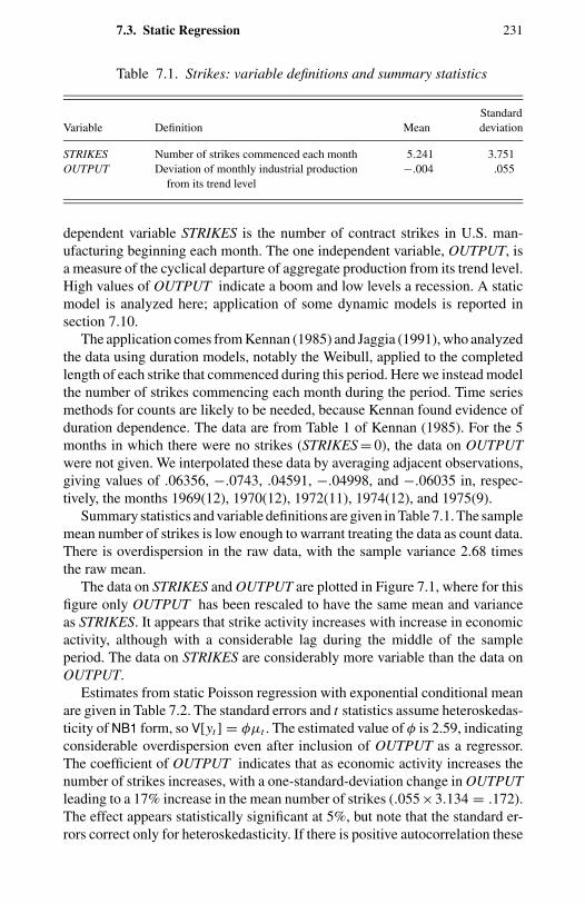
7.3. Static Regression 231

Table 7.1. Strikes: variable definitions and summary statistics

StandardVariable Definition Mean deviation

STRIKES Number of strikes commenced each month 5.241 3.751OUTPUT Deviation of monthly industrial production −.004 .055

from its trend level

dependent variable STRIKES is the number of contract strikes in U.S. man-ufacturing beginning each month. The one independent variable, OUTPUT, isa measure of the cyclical departure of aggregate production from its trend level.High values of OUTPUT indicate a boom and low levels a recession. A staticmodel is analyzed here; application of some dynamic models is reported insection 7.10.

The application comes from Kennan (1985) and Jaggia (1991), who analyzedthe data using duration models, notably the Weibull, applied to the completedlength of each strike that commenced during this period. Here we instead modelthe number of strikes commencing each month during the period. Time seriesmethods for counts are likely to be needed, because Kennan found evidence ofduration dependence. The data are from Table 1 of Kennan (1985). For the 5months in which there were no strikes (STRIKES = 0), the data on OUTPUTwere not given. We interpolated these data by averaging adjacent observations,giving values of .06356, −.0743, .04591, −.04998, and −.06035 in, respec-tively, the months 1969(12), 1970(12), 1972(11), 1974(12), and 1975(9).

Summary statistics and variable definitions are given in Table 7.1. The samplemean number of strikes is low enough to warrant treating the data as count data.There is overdispersion in the raw data, with the sample variance 2.68 timesthe raw mean.

The data on STRIKES and OUTPUT are plotted in Figure 7.1, where for thisfigure only OUTPUT has been rescaled to have the same mean and varianceas STRIKES. It appears that strike activity increases with increase in economicactivity, although with a considerable lag during the middle of the sampleperiod. The data on STRIKES are considerably more variable than the data onOUTPUT.

Estimates from static Poisson regression with exponential conditional meanare given in Table 7.2. The standard errors and t statistics assume heteroskedas-ticity of NB1 form, so V[yt ] = φµt . The estimated value of φ is 2.59, indicatingconsiderable overdispersion even after inclusion of OUTPUT as a regressor.The coefficient of OUTPUT indicates that as economic activity increases thenumber of strikes increases, with a one-standard-deviation change in OUTPUTleading to a 17% increase in the mean number of strikes (.055×3.134 = .172).The effect appears statistically significant at 5%, but note that the standard er-rors correct only for heteroskedasticity. If there is positive autocorrelation these

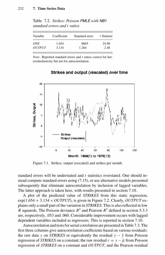
232 7. Time Series Data

Table 7.2. Strikes: Poisson PMLE with NB1standard errors and t ratios

Variable Coefficient Standard error t Statistic

ONE 1.654 .0665 24.90OUTPUT 3.134 1.264 2.48

Note: Reported standard errors and t ratios correct for het-eroskedasticity but not for autocorrelation.

Figure 7.1. Strikes: output (rescaled) and strikes per month.

standard errors will be understated and t statistics overstated. One should in-stead compute standard errors using (7.15), or use alternative models presentedsubsequently that eliminate autocorrelation by inclusion of lagged variables.The latter approach is taken here, with results presented in section 7.10.

A plot of the predicted value of STRIKES from this static regression,exp(1.654 + 3.134 × OUTPUT), is given in Figure 7.2. Clearly, OUTPUT ex-plains only a small part of the variation in STRIKES. This is also reflected in lowR squareds. The Poisson deviance R2 and Pearson R2 defined in section 5.3.3are, respectively, .053 and .060. Considerable improvement occurs with laggeddependent variables included as regressors. This is reported in section 7.10.

Autocorrelation and tests for serial correlation are presented in Table 7.3. Thefirst three columns give autocorrelation coefficients based on various residuals:the raw data y on STRIKES or equivalently the residual y − y from Poissonregression of STRIKES on a constant; the raw residual r = y − µ from Poissonregression of STRIKES on a constant and OUTPUT; and the Pearson residual

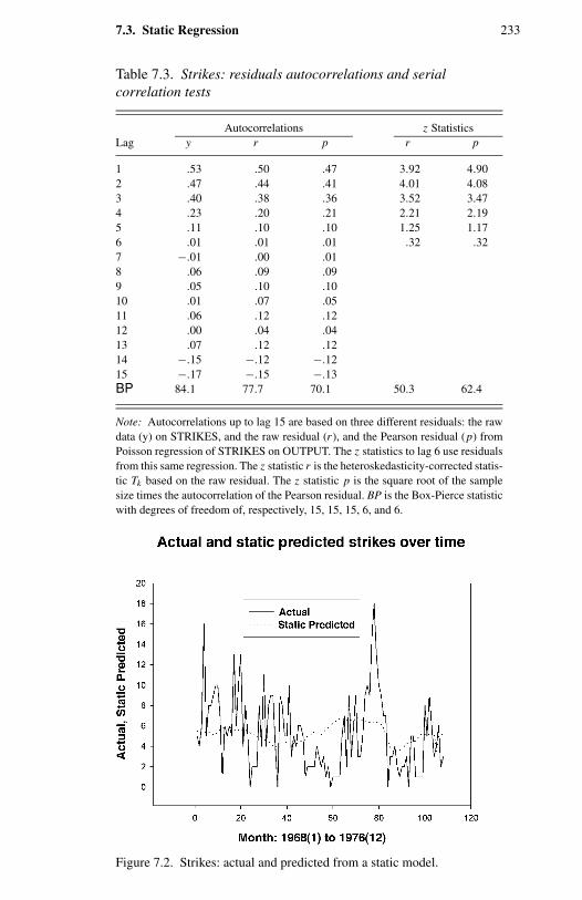
7.3. Static Regression 233

Table 7.3. Strikes: residuals autocorrelations and serialcorrelation tests

Autocorrelations z StatisticsLag y r p r p

1 .53 .50 .47 3.92 4.902 .47 .44 .41 4.01 4.083 .40 .38 .36 3.52 3.474 .23 .20 .21 2.21 2.195 .11 .10 .10 1.25 1.176 .01 .01 .01 .32 .327 −.01 .00 .018 .06 .09 .099 .05 .10 .1010 .01 .07 .0511 .06 .12 .1212 .00 .04 .0413 .07 .12 .1214 −.15 −.12 −.1215 −.17 −.15 −.13BP 84.1 77.7 70.1 50.3 62.4

Note: Autocorrelations up to lag 15 are based on three different residuals: the rawdata (y) on STRIKES, and the raw residual (r ), and the Pearson residual (p) fromPoisson regression of STRIKES on OUTPUT. The z statistics to lag 6 use residualsfrom this same regression. The z statistic r is the heteroskedasticity-corrected statis-tic Tk based on the raw residual. The z statistic p is the square root of the samplesize times the autocorrelation of the Pearson residual. BP is the Box-Pierce statisticwith degrees of freedom of, respectively, 15, 15, 15, 6, and 6.

Figure 7.2. Strikes: actual and predicted from a static model.

234 7. Time Series Data

p = (y − µ)/√

µ from this regression. Because there is relatively little vari-ability in µ around y (see Figure 7.2), in this application we expect the autocor-relations to tell a similar story, even though those based on the Pearson residualare theoretically preferred.

All three indicate autocorrelation that dies out after five lags. Individual teststatistics for autocorrelation at each lag are presented in the last two columnsof Table 7.3. These are asymptotically N[0, 1] distributed under the null hy-pothesis of no autocorrelation. The first measure uses the Pearson residualsand the result (7.19) for standardized residuals. The second measure uses theraw residuals and the more general result (7.21). Note that the first measureassumes that the conditional variance is proportional to the conditional mean,while the second measure leaves the conditional variance unspecified. The twolead to very similar conclusions. At the 5% significance level there is statisti-cally significant autocorrelation through the first four lags. This is highly jointlysignificant, using the Box-Pierce test reported in the last row of Table 7.3. Forthe first four columns this is TBP in (7.20), which is chi-squared distributed onlyfor column four. For the fifth column this is T ∗

BP in (7.22). Clearly time seriesmethods are called for.

7.4 Integer-Valued ARMA Models

The preceding section considered static count regression models, where the goalis to perform valid statistical inference and place minimal structure on any serialcorrelation. In the remainder of this chapter we consider more explicit modelsof this serial correlation. The first model presented is fully parametric and hasthe same serial correlation structure as linear ARMA models for continuousdata.

INARMA models specify the realized value of yt to be the sum of a countrandom variable whose value depends on past outcomes and the realization ofan iid count random variable εt whose value does not depend on past outcomes.This model is similar to the linear model yt = ρyt−1 +εt , for example, althoughit explicitly models yt as a count. Different choices of the distribution for εt

lead to different marginal distributions for yt , such as the Poisson. The modelhas the attraction of having the same serial correlation structure as linear ARMAmodels for continuous data.

INARMA models were independently proposed by McKenzie (1986) andAl-Osh and Alzaid (1987), for the pure time series case, and extended to theregression case by Brannas (1995a). They build on earlier work for continuousnon-Gaussian time series, specifically exponential and gamma distributions.See Jacobs and Lewis (1977) and further references in Lewis (1985).

7.4.1 Pure Time Series Models

We begin with the pure time series case, before introducing other regressors xt

in the next subsection. Let Y(t−1) = (yt−1, yt−2, . . . , y0). The simplest example

7.4. Integer-Valued ARMA Models 235

is the INAR(1) process

yt = ρ yt−1 + εt , 0 ≤ ρ < 1, (7.24)

where εt is an iid latent count variable independent of Y(t−1). The symbol denotes the binomial thinning operator of Steutel and Van Harn (1979), wherebyρ yt−1 is the realized value of a binomial random variable with yt−1 trials andprobability ρ of success on each trial. More formally ρ y =∑y

j=1 u j , whereu j is a sequence of iid binary random variables that take value 1 with probabilityρ and value 0 with probability 1 − ρ. Thus each of the y components surviveswith probability ρ, and dies with probability 1 − ρ.

First consider the unconditional distribution of y. It can be shown that

µ = E[y] = E[ε]

1 − ρ, (7.25)

and

σ 2 = V[y] = ρE[ε] + V[ε]

1 − ρ2, (7.26)

(see for example Brannas, 1995a, and exercise 7.3). Given a particular distri-bution for ε, the unconditional stationary distribution for y can be found byprobability generating function techniques; see Steutel and Van Harn (1979)and McKenzie (1986). For example, y is Poisson if ε is Poisson.

For the conditional distribution, taking the conditional expectation of (7.24)yields the conditional mean

µt | t−1 = E[yt | yt−1] = ρyt−1 + E[εt ], (7.27)

a result similar to that for the Gaussian model. The conditional variance is

σ 2t | t−1 = V[yt | yt−1] = ρ(1 − ρ)yt−1 + V[εt ]. (7.28)

The key step in obtaining (7.27) and (7.28) is to note that ρ yt−1, conditionalon yt−1, has mean ρyt−1 and variance ρ(1 − ρ)yt−1 using standard results onthe binomial with yt−1 trials.

It can be shown that the autocorrelation at lag k is ρk . Thus the INAR(1)model has the same autocorrelation function as the AR(1) model for continuousdata. The conditional distribution of yt given yt−1 is that of a Markov chain.

The Poisson INAR(1) model results from specifying the latent variable εt

in (7.24) to be iid Poisson with parameter λ. Then yt is unconditionally Pois-son with parameter λ/(1 − ρ). Furthermore, in this case (yt , yt−1) is bivariatePoisson, defined in Chapter 8. The conditional moments using (7.27) and (7.28)are

µt | t−1 = ρyt−1 + λ

σ 2t | t−1 = ρ(1 − ρ)yt−1 + λ,

(7.29)

236 7. Time Series Data

so the Poisson INAR(1) model is conditionally underdispersed. The transitionprobabilities for the Markov chain conditional distribution are

Pr [yt | yt−1] = exp(−λ)min(yt ,yt − 1)∑

j=0

λyt − j

(yt − j)!

(yt−1

j

)ρ j (1 − ρ)yt − 1 − j .

(7.30)

Generalizations of Poisson INAR(1) to INAR(p) and INARMA(p, q) modelsand to marginal distributions other than Poisson are given in various papersby McKenzie and by Al-Osh and Alzaid; Al-Osh and Alzaid additionally con-sidered estimation. See also Jin-Guan and Yuan (1991). McKenzie (1986) ob-tained an INARMA model with an unconditional NB model distribution for yt

by specifying εt to be iid NB. McKenzie (1988) studied the Poisson INARMAmodel in detail. Al-Osh and Alzaid (1987) considered estimation of the Pois-son INAR(1) model and detailed properties of INAR(1) and INAR(p) modelsin Alzaid and Al-Osh (1988, 1990, respectively). Alzaid and Al-Osh (1993)obtained an INARMA model with an unconditional generalized Poisson dis-tribution (see section 4.4.5), which potentially permits underdispersion. Thismodel specifies εt to be generalized Poisson and replaces the binomial thinningoperator by quasibinomial thinning. Although the INARMA models have thesame autocorrelation function as linear ARMA models, the partial autocorrela-tion functions differ.

Further models are given by Gauthier and Latour (1994), who define a gener-alized Steutel–Van Harn operator. Still further generalization may be possible.In the AR(1) case, for example, essentially all that is needed is an operator thatyields a discrete value for the first term in the right-hand side of (7.24). Forexample, there is no reason why the yt−1 trials need be independent, and onecould, for example, use a correlated binomial model.

Research on INARMA models has focused on stochastic properties. Lessattention has been paid to estimation. In the pure time series case exact MLE, aswell as conditional MLE which conditions on an initial value y1, were proposedand investigated by Al-Osh and Alzaid (1987) and Ronning and Jung (1992)for the Poisson INAR(1) model. These estimators can be difficult to implement,especially for models other than the Poisson.

An alternative estimator is conditional least squares. For the Poisson INAR(1)model, E[yt | yt−1] = ρyt−1 + λ. This allows simple estimation of ρ and λ byOLS regression of yt on an intercept and yt−1, a method proposed by Al-Oshand Alzaid (1987). The error in this regression is heteroskedastic, becauseV[yt | yt−1] = ρ(1 − ρ)yt−1 + λ, so care needs to be taken to obtain the correctvariance matrix, and the estimator could potentially be quite inefficient.

Brannas (1994) proposed and investigated the use of GMM estimators forthis model. GMM has the theoretical advantage of incorporating more of themoment restrictions, notably autocovariances, implied by the Poisson INAR(1)model than simply the conditional mean, or conditional mean and variance inthe case of conditional WLS.

7.4. Integer-Valued ARMA Models 237

None of these studies include exogenous regressors, with the exception ofMcKenzie (1985, p. 649), who briefly considered introduction of trends.

7.4.2 Regression Models

Brannas (1995a) proposed a Poisson INAR(1) regression model, with regressorsintroduced into (7.24) through both the binomial thinning parameter ρ and thelatent count variable εt . Thus

yt = ρt yt−1 + εt . (7.31)

The latent variable εt in (7.31) is assumed to be Poisson-distributed with mean

λt = exp(x′

tβ). (7.32)

To ensure 0 < ρt < 1, the logistic function is used

ρt = 1

1 + exp(−z′

tγ) . (7.33)

From (7.27) with ρ replaced by ρt , the conditional mean for this model is

µt | t−1 = E[yt | xt , zt , yt−1] =(

1

1 + exp(−z′

tγ)) yt−1 + exp

(x′

tβ).

(7.34)

A simpler specification sets zt = 1, so the parameter ρ is a constant. The con-ditional variance is

σ 2t | t−1 = V[yt | xt , zt , yt − 1] =

(exp(−z′

tγ)[

1 + exp(−z′

tγ)]2)

yt−1 + exp(x′

tβ),

(7.35)

from (7.35).Brannas proposed estimation of this model by conditional least squares and

by GMM. Using (7.34), the conditional NLS estimator minimizes with respectto β and γ

S(β,γ) =T∑

t=1

yt −

(1

1 + exp(−z′

tγ)) yt−1 − exp

(x′

tβ)2

,

(7.36)

where the usual standard errors need to be adjusted to allow for heteroskedas-ticity. This estimator is relatively straightforward to implement given access toa statistical package that includes NLS estimation, although reported standarderrors and t statistics may assume a homoskedastic error. An alternative, moreefficient estimator is conditional WLS, where the weighting function can beobtained from (7.35).

238 7. Time Series Data

Brannas also proposed estimating β and γ by GMM, using knowledge ofthe functional form for the autocovariances implied by the Poisson INAR(1)model. Details of the GMM procedure, which is considerably more complexto implement than conditional least squares, are given in Brannas (1995a). Hefound little gain from performing GMM rather than conditional least squares.

Brannas additionally considered prediction from this model. In an applica-tion to annual Swedish data on the number of paper mills of a particular type,the parameters γ in ρt are interpreted as representing the role of regressors inexplaining the death of firms; the parameters β of the Poisson density for εt

represent the role of regressors in explaining the birth of firms.

7.5 Autoregressive Models

The most direct method to specify a time series model is to specify a stan-dard count regression model, where analysis is conditional on past outcomesas well as current and past values of exogenous variables. Thus the condi-tioning set is now (X(t), Y(t−1)) where X(t) = (xt , xt−1, . . . , x0) and Y(t−1) =(yt−1, yt−2, . . . , y0).

The simplest model specifies an exponential conditional mean, where yt−1

additionally appears as a regressor. So the conditional mean is exp(x′tβ+ρyt−1).

This model may not be practically useful, however, as it is explosive for ρ > 0.Simulations and discussion are given in Blundell, Griffith, and Windmeijer(1995), who call this model exponential feedback. A better and more naturalmodel specifies a multiplicative role for yt−1, i.e.,

µt | t−1 = E[yt | X(t), Y(t−1)]

= exp(x′

tβ + ρ ln y∗t−1

)= exp

(x′

tβ)(

y∗t−1

)ρ, (7.37)

where y∗t−1 is a transformation of yt−1, such as (7.38) or (7.39), that is strictly

positive. This transformation is needed, as otherwise yt−1 = 0 is an absorbingstate, because then µt | t−1 = 0 and hence yt = 0 in fully parametric modelsfor yt such as P[µt | t−1]. Possibilities for y∗

t−1 include rescaling only the zerovalues of yt−1 to a constant c

y∗t−1 = max(c, yt−1), 0 < c < 1, (7.38)

and translating all values of yt−1 by the same amount

y∗t−1 = yt−1 + c, c > 0. (7.39)

The model (7.37) can be viewed as a multiplicative AR(1) model, by comparisonwith the linear AR(1) model in (7.1). We can also consider a multiplicative AR(1)

7.5. Autoregressive Models 239

error model

µt | t−1 = E[yt | X(t), Y(t−1)]

= exp(x′

tβ + ρ(

ln y∗t−1 − x′

t−1β))

= exp(x′

tβ) ( y∗

t−1

x′t−1β

)ρ

. (7.40)

By comparison the linear AR(1) error model from (7.6) implies µt | t−1 = x′tβ+

ρ(yt−1 − x′t−1β).

Models (7.37) and (7.40) were proposed by Zeger and Qaqish (1988) forGLM models, with the exponential function more generally replaced by thecanonical link function. The model was called a Markov model, here Markovmodel of order 1, because yt−1 is the only element of the past history Y(t−1)

that affects the conditional distribution of yt . An alternative terminology, usedhere, is to call this model an autoregressive model, given its obvious similarityto the linear model (7.2) and to avoid possible confusion with hidden Markovmodels.

Given the conditional mean specification in (7.37), estimation can be byNLS, the only complication being finding consistent standard errors. Providedthere is no serial correlation in the model residual yt − µt | t−1, these can beobtained using (7.13) with ωt j = 0 for j > 0.

If the conditional density is specified, for example, f (yt | xt , yt−1) is Poisson,then estimation can be by maximum likelihood, which maximizes

L =T∑

t=1

f (yt | xt , yt−1). (7.41)

Estimation theory is given in Wong (1986) and Fahrmeir and Kaufman (1987).Overdispersion could be handled by instead specifying f (yt | xt , yt−1) to be theNB2 density.

Zeger and Qaqish (1988) used quasilikelihood methods, an intermediate ap-proach between NLS and maximum likelihood estimation. In particular, obtainthe Poisson PMLE assuming that yt | xt , yt−1 is distributed as P[µt | t−1], whereµt | t−1 is given in (7.37). Then if the conditional variance specification is relaxedto the NB1 form V[yt | xt , yt−1] = φµt | t−1, the computed Poisson maximumlikelihood standard errors can be rescaled by φ1/2 as in section 3.2.3.

If the constant c in (7.38) or (7.39) is specified, then a standard Poissonprogram can be used. If instead c is an additional parameter to be estimated,standard Poisson software can still be used for y∗

t = max(c, yt−1) as in (7.38).Rewrite (7.40) as

µt | t−1 = exp(x′

tβ + ρ ln y∗∗t−1 + (ρ ln c) dt

)

240 7. Time Series Data

where

y∗∗t−1 = yt−1 and dt = 0, yt−1 > 0,

y∗∗t−1 = 1 and dt = 1, yt−1 = 0.

Poisson regression of yt on xt , y∗∗t−1 and dt yields estimates of β, ρ, and ρ ln c.

Then use c = exp[(ρ ln c)/ρ] to obtain an estimate of c. The autoregressivecount model is attractive because it is relatively simple to implement.

A weakness of the model is that adjustments such as (7.38) or (7.39) for zerolagged values of yt are ad hoc. Furthermore, they complicate evaluation of theimpact of regressors on the change in the conditional mean. One alternative isto replace (7.37) by

µt | t−1 = ρyt−1 + x′tβ. (7.42)

This equals the conditional mean (7.34) of the Poisson INAR(1) model if ρ

is constant, although other features of the distribution such as the conditionalvariance (see [7.35]) will differ. A major reason for choosing the exponentialconditional mean specification is to ensure a positive mean. This is also the casefor µt | t−1 in (7.42), provided ρ > 0. Another alternative to adjustments suchas (7.38) or (7.39), proposed by Shephard (1995), is to develop autoregressivemodels for a particular transformation of the dependent variable.

Autoregressive models have not been widely applied, especially for datafor which some counts are zero. Fahrmeir and Tutz (1994, section 6.1) gavean application to monthly U.S. data on the number of polio cases. Cameronand Leon (1993) applied the model to monthly U.S. data on the number ofstrikes and give some limited simulations to investigate the properties of bothestimators and the time series process itself, because theoretical results onits serial correlation properties are not readily obtained. Leon and Tsai (1998)proposed and investigated by simulation quasilikelihood analogues of LM, Wald,and LR tests, following the earlier study by Li (1991), who considered the LMtest.

7.6 Serially Correlated Error Models

The preceding models provide a fairly explicit model for dependence of yt

on past outcomes. Zeger (1988) instead introduced serial correlation in yt viaserial correlation in a multiplicative latent variable. This model is like the staticregression model studied in section 7.3. More structure is placed on the modelhere, however, leading to autocorrelations that are a function of current andlagged values of µt . This permits more efficient estimation than in section 7.3,assuming that the autocorrelations are correctly specified.

For counts the Poisson is used as a starting point, with variance equal to themean. The conditional distribution of the dependent variable yt is specified tobe independent over t with mean λtεt and variance λtεt , where conditioning is

7.6. Serially Correlated Error Models 241

on both regressors, via

λt = exp(x′

tβ),

and an unobserved latent variable εt > 0. The moments conditional on obser-vation of εt are

E[yt | λt , εt ] = λtεt (7.43)

V[yt | λt , εt ] = λtεt .

This setup is similar to the mixture models in Chapter 4. Here, however, thelatent variable is not independently distributed across observations and, ratherthan integrating out to get a density, just the first and second moments areobtained.

The latent variable εt is assumed to follow a stationary process with meannormalized to unity, variance σ 2, and covariances Cov[εt , εt−k] = ρkεσ

2, where

ρkε = Cor[εt , εt−k], k = 1, 2, . . . (7.44)

is the autocorrelation function for εt . It follows that the marginal distribution ofyt , marginal with respect to εt but still conditional on λt , has first two moments

µt = E[yt | λt ] = λt

σ 2t = V[yt | λt ] = λt + σ 2λ2

t .(7.45)

The latter result uses

V[y | λ] = E[V[y | λ, ε] | λ] + V[E[y | λ, ε] | λ]

= E[λε | λ] + V[λε | λ]

= λE[ε] + λ2V[ε].

The covariance between yt and yt−k can be shown to equal ρkεσ2t λtλt−k , im-

plying that the autocorrelation function for yt is

ρkyt = ρkε√(1 + 1

σ 2λ2t

) (1 + 1

σ 2λ2t−k

) , k = 1, 2, . . . . (7.46)

We refer to this model as a serially correlated error model because of itsobvious connection to the linear model in (7.4) and (7.5). Other authors refer tothis as a marginal model, because from (7.45) we model µt = exp(x′

tβ), whichdoes not condition on lagged yt .

Maximum likelihood estimation requires specification of both the densityfor yt given εt , and a multivariate density for (ε1, . . . , εT )′. No closed-formsolution is possible, except in trivial cases such as εt iid gamma if yt | εt iidPoisson, which gives independent NB.

242 7. Time Series Data

Instead a quasilikelihood approach is taken, using knowledge of the mean,variance, and covariances of yt . The nonlinear WLS estimator for β solves thefirst-order conditions

D′V−1(y − λ) = 0, (7.47)

where D is the T × k matrix with t j th element ∂λt/∂β j , V−1 is a T × Tweighting matrix, y is the T × 1 vector with t thentry yt and λ is the T × 1vector with t th entry λt . This is the same as the linear WLS estimator given insection 2.4.1, X′V−1(y − X′β) = 0, except that in moving to nonlinear modelsxt j in X is replaced by ∂λt/∂β j in D and the mean X′β is replaced by λ. Thenby results similar to section 2.4.1,βWLS is asymptotically normal with mean βand variance

V[βWLS] = (D′V−1D)−1D′V−1V−1′D (D′V−1D)−1, (7.48)

where Ω=Ω(β,γ, σ 2) is the covariance matrix of y, and γ are parameters ofthe autocorrelation function ρkε.

The efficient nonlinear WLS estimator is nonlinear feasible GLS whereV−1 = Ω

−1, and Ω is a consistent estimator of Ω=Ω(β,γ, σ 2). This entails

inversion of the T ×T estimated covariance matrix of yt , which poses problemsfor large T . Zeger instead proposed using less efficient WLS, where the workingweighting matrix V−1 is chosen to be reasonably close to Ω−1.

Zeger (1988) applied this method to monthly U.S. data on polio cases;Campbell (1994) applied this model to daily U.K. data on sudden infant deathsyndrome cases and the role of temperature.

Brannas and Johansson (1994) study the Zeger (1988) model in furtherdetail. In particular, they observe that in this model the usual Poisson PMLE isstill consistent. They find that the Poisson PMLE yields quite similar estimatesand efficiency to estimates using Zeger’s method, once appropriate correctionfor serial correlation is made to the Poisson PMLE standard errors. Johansson(1995) presents Wald- and LM-type tests based on GMM estimation (see Neweyand West, 1987b) for overdispersion and serial correlation in the Zeger modeland investigates their small-sample performance by a Monte Carlo study.

7.7 State-Space Models

The INAR and Markov models specify the conditional distribution of yt todepend on a specified function of (X(t), Y(t−1)). The state-space model or time-varying parameters model instead specifies the conditional distribution of yt todepend on stochastic parameters that evolve according to a specified distributionwhose parameters are determined by (X(t), Y(t−1)).

Analytical results are most easily obtained if only the mean parameterevolves over time, with density that is conjugate to the density of yt . We beginwith this case.

7.7. State-Space Models 243

More generally the regression coefficients may all evolve over time, in whichcase a normal distribution is typically chosen. Analytical results are then nolonger attainable, but recent advances in computer power and in computationalalgorithms mean that this is no longer an obstacle to empirical work. Developingthese computational algorithms is a very active area, some of which is touchedon in this section and in section 9.4, in which Poisson models with Gaussianrandom effects are discussed.

Much of the work with random coefficient models, such as time-varyingparameters, has been done in a Bayesian framework. Then interest lies in ob-taining the posterior mean, which in the time series case is used to generateforecasts that incorporate prior information. A standard reference is West andHarrison (1997). The computational methods developed for Bayesian analysisare also widely used in frequentist analyses in which the focus is on param-eter estimation, and it is not uncommon to see frequentist analyses take on aBayesian flavor because of this. We focus on the frequentist interpretation here.

7.7.1 Conjugate Distributed Mean

West, Harrison, and Migon (1985) propose Bayesian time series models forregression models with prior density for the conditional mean chosen to beconjugate to an LEF density. These models are presented as an extension ofdynamic linear models (see West and Harrison, 1997), to the GLM framework,although this extension is not seamless. The concern is in obtaining the posteriormean and forecasts, given specified values for the prior density parameters.

Harvey and Fernandes (1989) study these models in a non-Bayesian frame-work and considered parameter estimation. The most tractable model for countdata is a Poisson–gamma model.

The starting point is a Poisson regression model, where yt conditional on µt

is P[µt ] distributed, so

f (yt | µt ) = e−µt µt/yt !. (7.49)

In a departure from earlier Poisson models, the mean parameter µt is modeledto evolve stochastically over time with distribution determined by past valuesof yt . A convenient choice of distribution is the gamma

f (µt | at | t−1, bt | t−1) = e−bµt µa−1t

(a)b−a, at | t−1 > 0, bt | t−1 > 0,

(7.50)

where a and b in (7.50) are evaluated at a = at | t−1 = ωat−1 and b = bt | t−1 =ωbt−1 and 0 < ω ≤ 1. The conditional density of yt given the observables Y(t−1)

is

f(yt | Y(t−1)

) =∫ ∞

0f (yt | µt ) f

(µt | Y(t−1)

)dµt . (7.51)

244 7. Time Series Data

From Chapter 4, f (yt | Y(t−1)) is the negative binomial with parameters at | t−1

and bt | t−1. Estimation of ω and the parameters of µt is by maximum likelihood,where the joint density of Y(t) is the product of the conditional densities (7.51).The Kalman filter is used to recursively build at | t−1 and bt | t−1.

Harvey and Fernandes (1989) apply this approach to count data on goalsscored in soccer matches, purse snatchings in Chicago, and van driver fatali-ties. They also obtain tractable results for negative binomial with parametersevolving according to the beta distribution and for the binomial model. Singhand Roberts (1992) consider count data models. Harvey and Shephard (1993)consider the general GLM class. Brannas and Johansson (1994) investigatesmall-sample performance of estimators. Johansson (1996) gives a substantiveregression application to monthly Swedish data on traffic accident fatalities,which additionally uses the model of Zeger (1988) discussed in section 7.6.

7.7.2 Normally Distributed Parameters

In these models the starting point can again be the Poisson regression model(7.49), except now µt = exp(x′

tβt ) where βt evolves according to

βt = Atβt−1 + υt , (7.52)

where

υt ∼ N[0,Σt ].

For this model there are no closed-form solutions. The development of nu-merical techniques for these models is an active area of research.

An example is Durbin and Koopman (1997), who model British data onvan driver fatalities. They first follow Shephard and Pitt (1997) in developinga Markov chain Monte Carlo method to numerically evaluate the likelihoodof the model. Durbin and Koopman (1997) then propose a faster procedurethat calculates the likelihood for an approximating linear Gaussian model byKalman filter techniques for linear models and then computes the true likelihoodas an adjustment to this.

7.8 Hidden Markov Models

Hidden Markov time series models specify different parametric models in dif-ferent regimes, in which the unobserved regimes evolve over time according toa Markov chain. Here we summarize results given in considerably more detailin MacDonald and Zucchini (1997).

For the model with m possible regimes let Ct , t = 1, . . . , T , denote a Markovchain on state-space 1, 2, . . . , m. Thus Ct = j if at time t we are in regime j .In the simplest case, considered here, Ct is an irreducible homogeneous Markovchain, with transition probabilities

γi j = Pr [Ct = j | Ct−1 = i] , i, j = 1, . . . , m, (7.53)

7.9. Discrete ARMA Models 245

which are time invariant. It is assumed that there exists a unique strictly positivestationary distribution

δ j = Pr [Ct = j] , j = 1, . . . , m, (7.54)

where the δ j are a function of γi j . For the Poisson hidden Markov model, itis assumed that the count data yt in each regime are Poisson distributed, withmean parameter that varies with exogenous variables and the regime

µt j = exp(x′

tβ j). (7.55)

The moments of yt , unconditional on Ct although still conditional on xt , canbe shown to be

E[yt | xt ] =m∑

j=1

δ jµt j (7.56)

E[y2

t | xt] =

m∑j=1

δ j(µt j + µ2

t j

)(7.57)

E[yt yt+k | xt ] =m∑

i=1

m∑j=1

δiγi j (k)µtiµt+k, j , (7.58)

where γi j (k) = Pr[Ct+k = j | Ct−1 = i] and t = 1, . . . , T . The autocorrelationfunction of yt , which follows directly from (7.56) through (7.58), is a functionof the Poisson parameters and the transition probabilities.

The parameters to be estimated are the regime-specific parameters β j , j =1, . . . , m, and the transition probabilities γi j . Estimation by maximum likeli-hood, imposing the constraints that γi j ≥ 0 and the constraints

∑j =i γi j ≤ 1,

i = 1, . . . m, is presented in MacDonald and Zucchini (1997). Applications tocount data include the daily number of epileptic seizures by a particular pa-tient, fitted by a two-state hidden Markov Poisson model with µt j = µ j , andthe weekly number of firearm homicides in Cape Town, fitted by a two-statehidden Markov Poisson model with µt j = exp(α1 j + α2 j t + α3 j t2).

Count data can be directly modeled as a Markov chain, rather than via ahidden Markov chain. For counts there are potentially an infinite number oftransition parameters, and additional structure is needed. An example of suchstructure is the Poisson INAR(1) model, whose transition probabilities are givenin (7.30).

7.9 Discrete ARMA Models

The first serious attempt to define a time series count model with similar auto-correlation structure to ARMA models was by Jacobs and Lewis (1978a, 1978b,1983). They defined the class of DARMA models, for which the realized value

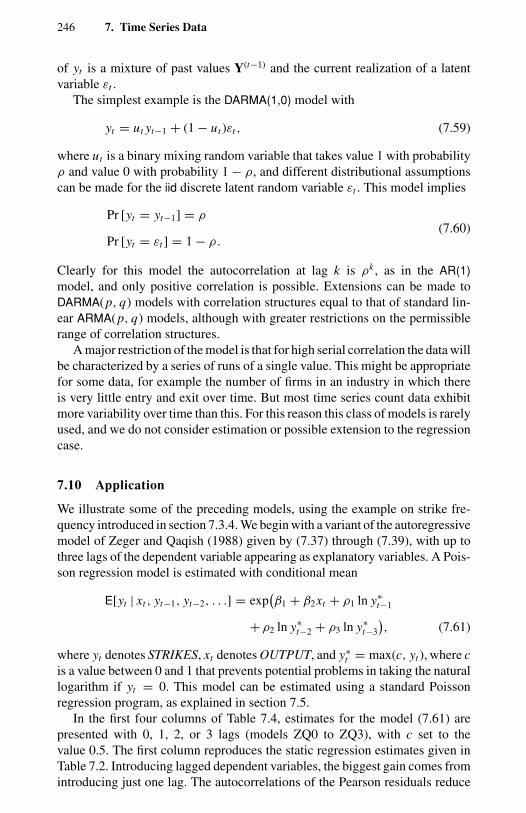
246 7. Time Series Data

of yt is a mixture of past values Y(t−1) and the current realization of a latentvariable εt .

The simplest example is the DARMA(1,0) model with

yt = ut yt−1 + (1 − ut )εt , (7.59)

where ut is a binary mixing random variable that takes value 1 with probabilityρ and value 0 with probability 1 − ρ, and different distributional assumptionscan be made for the iid discrete latent random variable εt . This model implies

Pr [yt = yt−1] = ρ

Pr [yt = εt ] = 1 − ρ.(7.60)

Clearly for this model the autocorrelation at lag k is ρk , as in the AR(1)model, and only positive correlation is possible. Extensions can be made toDARMA(p, q) models with correlation structures equal to that of standard lin-ear ARMA(p, q) models, although with greater restrictions on the permissiblerange of correlation structures.

A major restriction of the model is that for high serial correlation the data willbe characterized by a series of runs of a single value. This might be appropriatefor some data, for example the number of firms in an industry in which thereis very little entry and exit over time. But most time series count data exhibitmore variability over time than this. For this reason this class of models is rarelyused, and we do not consider estimation or possible extension to the regressioncase.

7.10 Application

We illustrate some of the preceding models, using the example on strike fre-quency introduced in section 7.3.4. We begin with a variant of the autoregressivemodel of Zeger and Qaqish (1988) given by (7.37) through (7.39), with up tothree lags of the dependent variable appearing as explanatory variables. A Pois-son regression model is estimated with conditional mean

E[yt | xt , yt−1, yt−2, . . .] = exp(β1 + β2xt + ρ1 ln y∗

t−1

+ ρ2 ln y∗t−2 + ρ3 ln y∗

t−3

), (7.61)

where yt denotes STRIKES, xt denotes OUTPUT, and y∗t = max(c, yt ), where c

is a value between 0 and 1 that prevents potential problems in taking the naturallogarithm if yt = 0. This model can be estimated using a standard Poissonregression program, as explained in section 7.5.

In the first four columns of Table 7.4, estimates for the model (7.61) arepresented with 0, 1, 2, or 3 lags (models ZQ0 to ZQ3), with c set to thevalue 0.5. The first column reproduces the static regression estimates given inTable 7.2. Introducing lagged dependent variables, the biggest gain comes fromintroducing just one lag. The autocorrelations of the Pearson residuals reduce

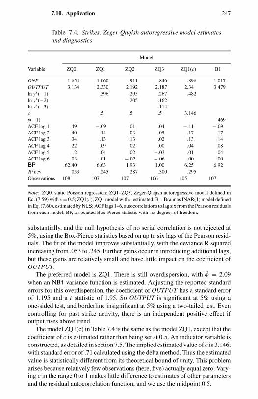
7.10. Application 247

Table 7.4. Strikes: Zeger-Qaqish autoregressive model estimatesand diagnostics

Model

Variable ZQ0 ZQ1 ZQ2 ZQ3 ZQ1(c) B1

ONE 1.654 1.060 .911 .846 .896 1.017OUTPUT 3.134 2.330 2.192 2.187 2.34 3.479ln y∗(−1) .396 .295 .267 .482ln y∗(−2) .205 .162ln y∗(−3) .114c .5 .5 .5 3.146y(−1) .469ACF lag 1 .49 −.09 .01 .04 −.11 −.09ACF lag 2 .40 .14 .03 .05 .17 .17ACF lag 3 .34 .13 .13 .02 .13 .14ACF lag 4 .22 .09 .02 .00 .04 .08ACF lag 5 .12 .04 .02 −.03 .01 .04ACF lag 6 .03 .01 −.02 −.06 .00 .00BP 62.40 6.63 1.93 1.00 6.25 6.92R2dev .053 .245 .287 .300 .295Observations 108 107 107 106 105 107

Note: ZQ0, static Poisson regression; ZQ1–ZQ3, Zeger-Qaqish autoregressive model defined inEq. (7.59) with c = 0.5; ZQ1(c), ZQ1 model with c estimated; B1, Brannas INAR(1) model definedin Eq. (7.60), estimated by NLS; ACF lags 1–6, autocorrelations to lag six from the Pearson residualsfrom each model; BP, associated Box-Pierce statistic with six degrees of freedom.

substantially, and the null hypothesis of no serial correlation is not rejected at5%, using the Box-Pierce statistics based on up to six lags of the Pearson resid-uals. The fit of the model improves substantially, with the deviance R squaredincreasing from .053 to .245. Further gains occur in introducing additional lags,but these gains are relatively small and have little impact on the coefficient ofOUTPUT.

The preferred model is ZQ1. There is still overdispersion, with φ = 2.09when an NB1 variance function is estimated. Adjusting the reported standarderrors for this overdispersion, the coefficient of OUTPUT has a standard errorof 1.195 and a t statistic of 1.95. So OUTPUT is significant at 5% using aone-sided test, and borderline insignificant at 5% using a two-tailed test. Evencontrolling for past strike activity, there is an independent positive effect ifoutput rises above trend.

The model ZQ1(c) in Table 7.4 is the same as the model ZQ1, except that thecoefficient of c is estimated rather than being set at 0.5. An indicator variable isconstructed, as detailed in section 7.5. The implied estimated value of c is 3.146,with standard error of .71 calculated using the delta method. Thus the estimatedvalue is statistically different from its theoretical bound of unity. This problemarises because relatively few observations (here, five) actually equal zero. Vary-ing c in the range 0 to 1 makes little difference to estimates of other parametersand the residual autocorrelation function, and we use the midpoint 0.5.

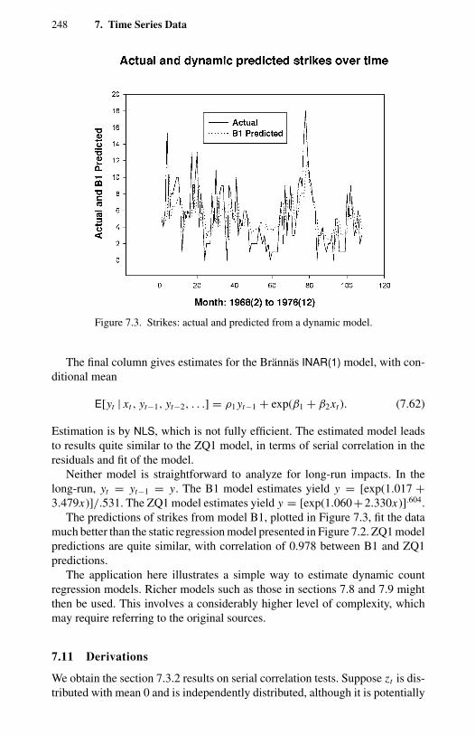
248 7. Time Series Data

Figure 7.3. Strikes: actual and predicted from a dynamic model.

The final column gives estimates for the Brannas INAR(1) model, with con-ditional mean

E[yt | xt , yt−1, yt−2, . . .] = ρ1 yt−1 + exp(β1 + β2xt ). (7.62)

Estimation is by NLS, which is not fully efficient. The estimated model leadsto results quite similar to the ZQ1 model, in terms of serial correlation in theresiduals and fit of the model.

Neither model is straightforward to analyze for long-run impacts. In thelong-run, yt = yt−1 = y. The B1 model estimates yield y = [exp(1.017 +3.479x)]/.531. The ZQ1 model estimates yield y = [exp(1.060+2.330x)].604.

The predictions of strikes from model B1, plotted in Figure 7.3, fit the datamuch better than the static regression model presented in Figure 7.2. ZQ1 modelpredictions are quite similar, with correlation of 0.978 between B1 and ZQ1predictions.

The application here illustrates a simple way to estimate dynamic countregression models. Richer models such as those in sections 7.8 and 7.9 mightthen be used. This involves a considerably higher level of complexity, whichmay require referring to the original sources.

7.11 Derivations

We obtain the section 7.3.2 results on serial correlation tests. Suppose zt is dis-tributed with mean 0 and is independently distributed, although it is potentially

7.11. Derivations 249

heteroskedastic. Then∑T

t=k+1 zt zt−k has mean

E

[T∑

t=k+1

zt zt−k

]= 0,

because E[zt zt−k] = 0, and variance

E

[T∑

s=k+1

T∑t=k+1

zs zs−k zt zt−k

]=

T∑t=k+1

E[z2

t z2t−k

],

using E[zt zuzvzw] = E[zt ]E[zuzvzw] by independence for t = u, v, w, andE[zt ] = 0. By a law of large numbers(

T∑t=k+1

E[z2

t z2t−k

])−1/2 T∑t=k+1

zt zt−kd→ N[0, 1], (7.63)

which yields (7.21) for tests on unstandardized residuals.Now specialize to the special case that zt is scaled to have constant variance,

in which case E[z2t ] is constant. Then

T∑t=k+1

E[z2

t z2t−k

] =T∑

t=k+1

E[z2

t

]E[z2

t−k

]

= 1

T

(T∑

t=k+1

E[z2

t

])( T∑t=k+1

E[z2

t−k

])

= 1

T

(T∑

t=k+1

E[z2

t

])( T∑t=k+1

E[z2

t

]),

where the first equality uses independence, and the second and third equal-ities use constancy of E[z2

t ]. It follows that ( 1T

∑Tt=1 z2

t )2 is consistent for1T

∑Tt=k+1 E[z2

t z2t−k], so

(1

T

T∑t=1

z2t

)−1 T∑t=k+1

zt zt−kd→ N[0, 1].

This implies T ρkd→ N[0, 1], as in (7.19), or equivalently the usual result that

ρk ∼ N[0, 1T ].

If E[z2t ] is nonconstant this simplification is not possible. One instead uses

1T

∑Tt=k+1 z2

t z2t−k as a consistent estimator of 1

T

∑Tt=k+1 E[z2

t z2t−k], and the more

general (7.21).

250 7. Time Series Data

7.12 Bibliographic Notes

An early treatment is Cox and Lewis (1966). McKenzie (1985) is a stimulatingpaper that raises, for counts, many standard time series issues, such as trendsand seasonality, in the context of hydrological examples. A recent survey ofcount time series models, which covers many of the models presented in thischapter, is given in Chapter 1 of MacDonald and Zucchini (1997). The bestreference for INARMA regression models is Brannas (1995a). Autoregressivemodels, serially correlated error models, and state-space models for GLMs arecovered in some detail in Fahrmeir and Tutz (1994, chapter 8). State-spacemodels, both linear and nonlinear, are discussed in Harvey (1989) and Westand Harrison (1997). Estimation of models with time-varying parameters is anactive area of research. Recent summaries of numerical methods include thosein Fahrmeir and Tutz (1994) and West and Harrison (1997). The hidden Markovmodel for count and binomial data is presented in detail by MacDonald andZucchini (1997).

7.13 Exercises

7.1 The first-order conditions for the Poisson PMLE are∑

t g(yt , xt ,β) = 0where g(yt , xt ,β) = (yt −exp(x′

tβ))xt . Apply the general result given in section2.7.1 to obtain (7.15) for yt heteroskedastic and autocorrelated to lag l.

7.2 Consider OLS regression of yt on scalar xt without intercept in the cross-section case. The robust sandwich heteroskedastic consistent estimate of thevariance of β is [

∑t x2

t ]−1 [∑

t (yt −xt β)2x2t ] [∑

t x2t ]−1. Specialize this formula

if there is no relationship between yt and xt (so β = 0), and obtain the result-ing formula for t = β/

√V[β]. Apply this result to the case of regression of zt

on zt−k and compare the formula with (7.21).

7.3 Suppose εt in (7.24) is iid. Then yt is stationary with, say, E[yt ] = µ for all tand V[yt ] = σ 2 for all t . Using the general result E[y] = Ex [E[y | x]], use (7.27)to obtain (7.25). Using the general result V[y] = Ex [V[y | x]] + Vx [E[y | x]],use (7.28) to obtain (7.26).

7.4 For the Poisson INAR(1) model give the objective function for the condi-tional WLS estimator discussed after (7.36) and obtain the variance matrix forthis estimator.

7.5 Show that the binomial thinning operator in section 7.4 implies 0 y = 0;1 y = y; E[α y] = αE[y]; and V[α y] = α2V[y] + α(1 − α)E[y]; and thatfor any γ ∈ [0, 1], γ α y = (γα) y, by definition.

7.6 Given (7.43) and the assumptions on εt , obtain (7.45) and (7.46).

CHAPTER 8

Multivariate Data

8.1 Introduction

In this chapter we consider regression models for an m-dimensional vector ofjointly distributed, and in general correlated, random variables y = (y1, y2, . . . ,

ym), a subset of which are event counts. A special case is if m = 2, y1 is a count,and y2 is either discrete or continuous. Multivariate data appear in three contextsin this book. The first is basic cross-section, which is the main subject of thischapter. The second is longitudinal data with repeated measures over time onthe same variable, leading to special correlation structure handled in Chapter 9.The third is the context of multivariate cross-section data with endogeneity orfeedback from yj to yk , dealt with in Chapter 10. There are other forms ofmultivariate data, such as multivariate time series analogs of Gaussian vectorautoregressions, that we do not cover.

Multivariate linear Gaussian models are widely used, but multivariate nonlin-ear, non-Gaussian models are less common. Fully parametric approaches basedon the joint distribution of non-Gaussian vector y, given a set of covariates x, aredifficult to apply because analytically and computationally tractable expressionsfor such joint distributions are available for special cases only. Consequently, itis more convenient to analyze models that are of interest in specific situations.

Multivariate cross-section count models arise in several different settings.The first is that in which several related events are measured as counts andthe joint distribution of several counts is required. These models are analogousto the seemingly unrelated regressions model. A second situation is one inwhich counted events are jointly determined with (but not by) other noncountvariables, which may be continuous or discrete. A third situation is one inwhich the model involves simultaneity between a count variable or variablesand another continuous or discrete variable, so the situation is analogous to thatin simultaneous equation models.

Empirical examples of each of the three situations are readily found. Forexample, a model of the frequency of entry and exit of firms to an industryis an example of a bivariate count process (Mayer and Chappell, 1992). Amodel of healthcare utilization using several measures of healthcare services(hospital admissions, days spent in hospitals, prescribed and nonprescribed

252 8. Multivariate Data

medicines) is an example of jointly dependent counts. An example of a jointmodel of counts and discrete choice variables is a model of the frequency ofrecreational trips and discrete choice of recreational sites (Terza and Wilson,1990; Hausman, Leonard, and McFadden, 1995). Examples of joint modelingof counts and continuous variables are provided by Meghir and Robin (1992)and van Praag and Vermeulen (1993), who model frequency of purchase andamount of purchase.

Applications of multivariate count models are relatively uncommon. Prac-tical experience has been restricted to some special computationally tractablecases. Section 8.2 discusses some approaches and general issues relevant tocharacterizing dependence. Section 8.3 deals with properties and maximumlikelihood–based estimation of parametric models, including bivariate Pois-son models, without or with unobserved heterogeneity. Section 8.4 considersmoment-based estimation of the bivariate and multivariate models with oneor more moment restrictions. Section 8.5 considers the orthogonal polynomialseries expansions as a way of characterizing and testing for dependence inmultivariate models. Section 8.6 considers mixed models with both counts andother continuous or discrete variables.

8.2 Characterizing Dependence

8.2.1 Some Approaches

Consider the standard decomposition of the joint distribution of a two-dimen-sional random variable (Y1, Y2), denoted by fY1,Y2 (y1, y2 | x), into conditionaland marginal distributions:

fY1,Y2 (y1, y2 | x) = fY1 | Y2 (y1 | y2, x) fY2 (y2 | x)

= fY2 | Y1 (y2 | y1, x) fY1 (y1 | x), (8.1)

where x denotes exogenous variables that may have overlapping elements.∗ Thedecomposition implies that if these densities exist, the joint distribution can bedefined using either product in the decomposition:

fY1 | Y2 (y1 | y2, x) fY2 (y2 | x) = fY2 | Y1 (y2 | y1, x) fY1 (y1 | x). (8.2)

The parameters of the joint distribution may be estimated using the joint dis-tribution, if it is available, or by working with the conditional and the marginaldistributions, which may be computationally more convenient.

Given conditional specifications fY1 | Y2 (y1 | y2, x) and fY2 | Y1 (y2 | y1, x), thejoint density may be defined if there exist proper marginals that satisfy (8.2).Because not all pairs of conditionals will be coherent in the sense of satisfying

∗ Elsewhere we have used f (y), f (y1, y2), and so forth as generic notation for density. The slightlydifferent notation used here distinguises between random variables and their realizations foradditional clarity.

8.2. Characterizing Dependence 253

(8.2), they are subject to some restrictions. In econometrics joint distributionsare of considerable interest because they have a key role in structural or causalmodeling. On the other hand, conditional distributions connect naturally to theregression models that are often a starting point of empirical investigations. Inempirical work it is not uncommon to both begin and end with a conditionalspecification, leaving unresolved the problem of finding a valid joint distribu-tion. Conditional modeling of interdependent variables is justifiable if there isa plausible recursive ordering of outcomes (decisions) that correspond to ob-served endogenous variables.† It is also a feasible and asymptotically efficientapproach in some cases, such as bivariate exponential class if the condition-als are also from a bivariate exponential class (Moschopoulos and Staniswalis,1994).

The terminology used here is econometric. Some additional clarificationmay be helpful for those less familiar with it. In this context a definition ofexogeneity, parallel to that used in time series econometrics (Hendry, 1995), hasan important role. Roughly, in modeling y1 the variables (y2, x) are exogenous ifthey are determined without reference to y1, which rules out contemporaneousor lagged feedback from y1 to y2. Because our focus is on cross-section datain this chapter, we are mainly concerned with contemporaneous feedback, orsimultaneity and interdependence.

For a more precise definition, first rewrite the conditional-marginal decom-position (8.1) by incorporating parameters as in

fY1,Y2 (y1, y2 | x,θ) = fY1 | Y2 (y1 | y2, x,φ1) fY2 (y2 | x,φ2),

where θ ∈ ⊂ Rk,φ≡ [φ1...φ2] = g(θ). If there are constraints connecting

elements of θ, they are incorporated in the joint distribution. The function g(θ)is a transformation of the parameters θ, with dim(θ) = dim(φ). The parametervector φ is partitioned into subsets φ1 and φ2, which appear in the conditionaland marginal densities, respectively. Note that association parameters that areincluded in θ may not be identified by carrying out conditional or marginalanalysis alone.

The conditioning set (y2, x) is said to be exogenous if φ1 is fully informativeaboutθ, or any subset ofθ. In this caseφ2 does not depend onφ1. Under this con-dition, it is valid to make inferences about φ1, or the relevant subset of θ, usingthe conditional model alone. No separate statistical modeling of y2 is necessary.

If (y1, y2) are mutually dependent, as in the simultaneous equations modelsof economics, there is feedback from y2 to y1. In this case inferences aboutthe change in y1 induced by changes in y2, based on the conditional modelalone, have limited validity. Modeling interdependent variables can be carriedout in different ways; a full specification and analysis of a joint distribution is

† The plausibility of recursivity as a justification for conditioning is not always obvious. Forexample: Does a rational household first determine the number of shoping trips and then theamount spent in each trip, or does it do so jointly?

254 8. Multivariate Data

one approach. Analyses of interdependent variables may be carried out usinga fully parametric specification of the joint distribution. This is called a fullinformation (maximum likelihood) approach. Interdependent variables mayalso be analyzed using a moment-based approach such as GMM. If dealingwith the statistical implications of stochastic dependence between variables,this approach does not require or use a full parametric specification of the jointdistribution and does not permit inferences about all parameters. Hence it is alimited information approach.

Models based on joint distributions or joint moments are said to be structuralif they correspond to autonomous behavioral relationships and incorporate rel-evant parametric constraints. Univariate and multivariate marginal models maynot permit identification of parameters θ. So a statistical analysis may be re-stricted to φ2 only.

A full information analysis requires a flexible joint distribution. This is oftennot feasible for general multivariate models with interdependent discrete andcontinuous variables. Even in special bivariate cases, parametric closed formjoint distributions may be obtainable only under restrictive conditions. In sec-tion 8.3 we consider some leading bivariate cases. If less restrictive situationsare considered, closed-form joint densities are often not available, and conse-quently the construction of a joint likelihood may proceed on a case-by-casebasis with many context-specific assumptions.

In marginal models, the dependence on covariates and the association be-tween the endogenous variables are modeled separately, not jointly. Modelingbased on marginal distributions may be handled using the methods developedin Chapters 3, 4, and 5, supplemented by methods for measuring associationamong jointly dependent variables, which are developed in this chapter. In em-pirical work, however, the choice of marginal distributions may be more orless arbitrary, and the investigation may not proceed to the derivation of theunderlying joint distribution, if it exists.

8.2.2 Example

We illustrate the issues raised in the preceding discussion of dependence char-acterization by reference to a specific example. A useful technique for inducingdependence is to introduce correlated unobserved heterogeneity in marginaldistributions. This approach has been used widely in bivariate LEF models. Forconcreteness, we consider an example that is empirically important and thatrecurs in Chapter 11. The discussion draws on Terza (1998) and Weiss (1995).

Consider two random variables (y1, y∗2 ) where y1 is a count variable. Sup-

pose, conditionally on xi andνi , y1i is distributed P[µi ], andµi = exp[x′iβ+ νi ].

Here νi represents unmeasured heterogeneity. It is an iid random variable in-dependent of xi . Suppose that y∗

2 is a normally distributed unobserved latentvariable,

y∗2i = z′

iδ + εi ,

8.2. Characterizing Dependence 255

where εi ∼ N[0, σ22], which is related to an observable binomial variable y2 in

the following way:

y2 =

0 if y∗2i < 0

1 if y∗2i ≥ 0.

Then an association between y1 and y2 is induced by association (correlation)between ν and ε. That is, the joint probability distribution of ν and ε determinesin part the joint probability distribution of y1 and y2.

The joint probability distribution of y1 and y2 is related to the joint probabilitydistribution of ν and ε. Suppose that this distribution is bivariate normal withcorrelation parameter ρ, and covariance matrix

Σ =(

1 ρσ2

ρσ2 σ22

)where the variance σ2

1 has been normalized to unity. The association between ε

and ν is characterized by

ν = ρε + η, (8.3)

where η is normally and independently distributed. Then the marginal den-sity of y1 is a Poisson–normal mixture,

∫f [y1 | X, ν]g(ν)dν, which cannot be

expressed in a closed form.First we consider a full information approach based on the joint distribution.

Suppose y2 has a binomial distribution, then the likelihood function is given by

L(Θ) =n∏

i=1

f (y1i , y2i )

=n∏

i=1

f (y1i , y2i = 1)y2i Pr[y1i , y2i = 0]1−y2i , (8.4)

where Θ contains all the parameters in the joint distribution.The expressions for probability on the right-hand side can be expressed as

integrals over the variable ν. Maximization of such a likelihood requires numer-ically intensive methods of computation. This is an obstacle to full informationanalysis. It is computationally more convenient to consider estimation basedon the decomposition given in (8.1).

We next consider a limited information approach based on specification ofconditional moments using the specification

y1i = exp[x′

iβ + αy2i]νi

y2i = E[y2i | zi ] + εi ,(8.5)

where y2 in the first equation must be regarded as an endogenous variablecorrelated with ν. A sequential two-step estimator estimates the first of the

256 8. Multivariate Data

above equations after replacing y2 by an estimate of E[y2 | x], which is uncor-related with ν. But computing this expectation requires the marginal densityof y2, which is often not available. In practice, therefore, the step may be im-plemented by an ad hoc procedure that uses “an” estimate (rather than “the”estimate) of conditional expectation, calculated by a first-step regression onvariables assumed uncorrelated with ν, which amounts to an instrumental vari-able procedure. Thus the equation of interest becomes

y1i = exp[x′

iβ + αE[y2i | zi ] − α(E[y2i | zi ] − E[y2i | zi ])]νi .

For example, for the binary y2 variable, the first stage could generate the fit-ted probability, a proxy for E[y2i | zi ], from a probit regression. The analysisof y1i would be conditional on stage-one estimates. This problem is furtheranalyzed in Chapter 11.

8.3 Parametric Models

8.3.1 Bivariate Poisson

Unlike the case of the normal distribution, there is no unique multivariate Pois-son. There are several ways in which a model with Poisson marginals can bederived. Often any distribution that leads to Poisson marginals is referred to asa multivariate Poisson.

A well-established technique for deriving multivariate (especially bivariate)count distributions is the method of mixtures and convolutions. The oldest andthe most studied special case is the bivariate Poisson model, which can begenerated by sums of independent random counts with common componentsin the sums, also called the trivariate reduction technique (Kocherlakota andKocherlakota, 1993). Suppose count variables y1 and y2 are defined as

y1 = u + w, (8.6)

y2 = v + w, (8.7)

and u, v, and w are independently distributed as Poisson variables with parame-ters µ1, µ2, and µ3, respectively, µ j > 0, j = 1, 2, 3. Then the joint frequencydistribution, which is derived in section 8.7, is given by

f (y1 = r, y2 = s) = exp(µ1 + µ2 + µ3)min(r,s)∑

l=0

µr−l1 µs−l

2 µl3

(r − l)!(s − l)!l!.

(8.8)

The marginals are, respectively,

y1 ∼ P[µ1 + µ3], (8.9)

8.3. Parametric Models 257

and

y2 ∼ P[µ2 + µ3], (8.10)

with the squared correlation given by

ρ2 = µ23

(µ1 + µ3)(µ2 + µ3), (8.11)

(see Johnson and Kotz, 1969). Allowing for heterogeneity by allowing theparameters to vary across individuals implies that the correlation between eventsalso varies across individuals. However, maximum correlation between y1 andy2 is given by µ3/[µ3 + min(µ1, µ2)]. Gourieroux et al. (1984b) present adifferent derivation of the bivariate Poisson.

The use of trivariate reduction technique leads to the following properties:

1. In general, in multivariate nonnormal distributions the correlation doesnot fully describe the dependence structure of variables. However, inthis special case the correlation coefficient fully characterizes depen-dence, and no additional measures of dependence are needed.

2. The marginal distributions for y1 and y2 are both Poisson. Hence, with acorrectly specified conditional mean function the marginal models canbe estimated consistently, but not efficiently, by maximum likelihood.Joint estimation is more efficient even if the two mean functions dependon the same covariates.

3. This model only permits positive correlation between counts.

Then the log-likelihood for the model is

L(µ1, µ2, µ3 | y1, y2, x) =n∑

i=1

µ3i −n∑

i=1

(µ1i + µ2i ) +n∑

i=1

ln Si ,

where

Si =min(y1i ,y2i )∑

l=0

µy1i −l1 µ

y2i −l2 µl

3

(y1i − l)!(y2i − l)!l!.

At this stage there are two ways to proceed. One approach parameterizes the sumµ1i + µ2i as an (exponential) function of xi . A second approach parameterizesµ1i and µ2i individually in terms of same or different covariates. The twoapproaches imply different specifications of the conditional means. Taking thesecond approach, assume that µ3i = µ3, µ1i = exp(x′

iβ) and µ2i = exp(x′iγ).

This leads to the log-likelihood

L(β,γ, µ3 | y1, y2, x) = nµ3 −n∑

i=1

(exp(x′

iβ)+ exp

(x′

iγ))

+n∑

i=1

ln Si .

258 8. Multivariate Data

King (1989a) calls this seemingly unrelated Poisson regression maximumlikelihood estimator (SUPREME) by analogy with the well-known seeminglyunrelated least squares model. Jung and Winkelmann (1993), in their applicationof the bivariate Poisson to the number of voluntary and involuntary job changes,assume a constant covariance and exponential mean parameterization for themarginal means so that µ j + µ3 = exp(x′

jβ j ), j = 1, 2; this allows the twomeans to depend on separate or common sets of covariates. This assumptionsubstituted into (8.8) provides the basis for deriving the joint likelihood of theunknown parameters.

Bivariate Poisson is a special case of the generalized exponential family(Jupp and Mardia, 1980; Kocherlakota and Kocherlakota, 1993)

f (y1, y2 | µ1, µ2, ρ) = expµ′

1v(y1) + v(y1)′ρw(y2) + µ′2w(y2)

− c(µ1, µ2, ρ) + d1(y1) + d2(y2)

(8.12)

where v(·), w(·), d1(·) and d2(·) are functions, and c(µ1, µ2, 0) = c1(µ1)c2(µ2).Under independence, ρ = 0, in which case the right-hand side is a product of twoexponential families. In this family ρ = 0 is a necessary and sufficient conditionfor independence. The correlation coefficient is increasing in µ3 and decreasingsteeply in both µ1 and µ2.

8.3.2 Other Fully Parametric Models

The bivariate Poisson can be generalized and extended to allow for unobservedheterogeneity and overdispersion in the respective marginal distributions usingmixtures and convolutions as in the univariate case.

Marshall and Olkin (1990) generate multivariate distributions from mix-tures and convolutions of product families in a manner analogous to equation(4.10), which leads to compound marginal distributions. Consider the bivariatedistribution

f (y1, y2 | x1, x2) =∫ ∞

0f1(y1 | x1, ν) f2(y2 | x2, ν)g(ν) dν, (8.13)

where f1, f2, and g are univariate densities, and ν may be interpreted as com-mon unobserved heterogeneity affecting both counts. Multivariate distributionsgenerated in this way have univariate marginals in the same family (Kocher-lakota and Kocherlakota, 1993). Thus, a bivariate negative binomial mixturegenerated in this way will have univariate negative binomial mixture densities.This approach suggests a way of specifying or justifying overdispersed andcorrelated count models, based on a suitable choice of g(·), more general thanin the example given above. Marshall and Olkin (1990) generate a bivariatenegative binomial distribution beginning with f (y1) and f (y2), which are Pois-son with parameters µ1ν and µ2ν, respectively; ν has gamma distribution with

8.3. Parametric Models 259

parameter α−1. That is,

h(y1, y2 | µ1, µ2, α−1) =

∫ ∞

0[(µ1ν)y1 exp(−µ1ν)/y1!]

× [(µ2ν)y2 exp(−µ2ν)/y2!][

να−1−1 exp(−ν)/(α−1)]dν

= (y1 + y2 + α−1

)y1!y2!(α−1)

[µ1

µ1 + µ2 + 1

]y1[

µ2

µ1 + µ2 + 1

]y2

×[

1

µ1 + µ2 + 1

]α−1

. (8.14)

The marginals are again univariate negative binomial and the correlation ispositive. After parameterizing (µ1, µ2) maximum likelihood estimation ap-pears feasible, but to date there do not appear to have been applications ordocumented computational experience. Note that a result of Lindeboom andvan den Berg (1994) for bivariate survival models indicates that it is hazardousto estimate bivariate models in which mutual dependence survival times arisepurely from unobserved heterogeneity characterized as a univariate randomvariable. This result is also likely to apply to bivariate count models, and it sug-gests the desirability of flexible handling of the correlation structure betweencounts.

More flexible bivariate and multivariate parametric count data models can beconstructed by introducing correlated, rather than identical, unobserved hetero-geneity components in models. For example, suppose y1 and y2 are, respectively,P[µ1 | ν1] and P[µ2 | ν2] with E[ν1] = E[ν2] = 1, and

µ1 = exp(β0 + ν1 + x′β1) (8.15)

and

µ2 = exp(β0 + ν2 + x′β2), (8.16)

where ν1 and ν2 represent unobserved heterogeneity; their presence inducesoverdispersion in the marginal distributions of y1 and y2. Dependence betweeny1 and y2 is induced if ν1 and ν2 are correlated. In these cases the marginaldistributions for y1 and y2 exhibit both overdispersion and dependence, butin general in such cases neither the joint nor the marginal distributions haveclosed-form expressions. The joint distribution can be derived by extending theapproach based on (8.13). For example, the assumption of common heterogene-ity may be replaced by a bivariate normal distribution of (ν1, ν2). Maximumlikelihood estimation of such models requires numerically intensive methods,such as numerical or Monte Carlo integration.

260 8. Multivariate Data

8.4 Moment-Based Estimation

8.4.1 Bivariate Poisson with Heterogeneity

We wish to allow jointly for departures from equidispersion and a flexible pat-tern of correlation between counts. But we also want a tractable estimation pro-cedure. With these motivations, Gourieroux et al. (1984b, pp. 716–717) proposea sequential moment-based procedure for a bivariate count model. Their modelis more general than the bivariate Poisson because it permits overdispersion inthe conditional distributions.

The pair (y1, y2) have a common additive stochastic component v as in

y1 = u + v

y2 = w + v,(8.17)

conditional on an unobserved component, respectively ν1, ν2, ν3, the componentrandom variables u,v andw are each Poisson distributed. The conditional meansand variances, suppressing the conditioning on x for notational simplicity, areas follows:

E[u | ν1] = exp(x′

1β1 + ν1)

E[v | ν2] = exp(x′

2β2 + ν2)

(8.18)

E[w | ν3] = exp(x′

3β3 + ν3),

E[yi |ν i ] =[

E[y1i | ν1i , v2i ]

E[y2i | ν2i , v3i ]

]

=[

exp(x′

1iβ1 + ν1i)+ exp

(x′

2iβ2 + ν2i)

exp(x′

2iβ2 + ν2i)+ exp

(x′

3iβ3 + ν3i)] , (8.19)

where, the unobserved components νi are assumed to have moments

E[ν i ] = E

ν1i

ν2i

ν3i

=

1

1

1

; V[ν i ] = Ω; i = 1, . . . , n. (8.20)

Define the (2 × 1) row vector y′i = (y1i , y2i ), i = 1, . . . , n, and (2 × 3) matrix

Mi =[

exp(x′

1iβ1

)exp(x′

2iβ2

)0

0 exp(x′

2iβ2

)exp(x′

3iβ3

)] . (8.21)

Further,

V[yi |ν i ] =[

exp(x′

1iβ1

)+ exp(x′

2iβ2

)exp(x′

2iβ2)

exp(x′

2iβ2

)exp(x′

2iβ2

)+ exp(x′

3iβ3)].

(8.22)

8.4. Moment-Based Estimation 261

Unconditionally, the first two moments of y are, respectively,

E[yi ] =[

E[y1i ]

E[y2i ]

]=[

exp(x′

1iβ1

)+ exp(x′

2iβ2

)exp(x′

2iβ2

)+ exp(x′

3iβ3

)] (8.23)

and

V[yi ] = Vi = V1i + MiΩM′i , (8.24)

where

V1i =[

exp(x′

1iβ1

)+ exp(x′

2iβ2

)exp(x′

2iβ2)

exp(x′

2iβ2

)exp(x′

3iβ3

)+ exp(x′

2iβ2)] ,

and

MiΩM′i =[

a2ω11+ abω21+ baω12+ b2ω22 baω12+ b2ω22+ caω13+ cbω23

abω21+ acω31+ b2ω22+ bcω32 b2ω22+ bcω32+ cbω23+ c2ω33

],

where a = exp(x′1iβ1), b = exp(x′

2iβ2), and c = exp(x′3iβ3) and ω jk is the jk th

entry of . This result is obtained by applying (4.4).Then the QGPML estimator of (β1,β2,β3) may be obtained by minimizing

n∑i=1

(yi − E[yi ])′V−1

i (yi − E[yi ]), (8.25)

where Vi is a consistent estimator of the variance of yi , denoted Vi .The two-step QGPML estimator can be computed by the following algorithm:

1. Obtain consistent estimates of (β1,β2,β3) using a method such asNLS, based on the conditional means given in (8.23). Use them toobtain consistent estimates (a, b, c).

2. Obtain a consistent estimator of the elements of Ω by auxiliary linearregressions of the distinct elements of the (2×2) matrix (Vi − V1i ) onthe corresponding elements of the (2×2) matrix MiΩM′

i (the elementsof Vi are squares or cross-products of raw residuals from step 1). Thisstep is suggested by the structure of the variance matrix as given inequation (8.24). For example, the regression of the (1, 1) element of(Vi −V1i ) on (a2, 2ab, b2) will yield estimates of ω11, ω21(=ω12), andω22.

3. Obtain an estimate of Vi by substituting (β1, β2, β3, Ω) into the ex-pression (8.24) for Vi .

4. Minimize the objective function (8.25) and obtain the asymptotic co-variance matrix by specializing the result (2.76) in Chapter 2.

This moment-based estimator is not entirely without problems. Note thatbecause the three regressions yield nine estimates of six distinct elements of Ω,

262 8. Multivariate Data

there is a problem of nonuniqueness. Further, the consistent estimates need notlead to a symmetric positive definite Ω required for second-stage estimation.The nonuniqueness problem can be tackled by estimating the auxiliary regres-sions as a system of three linear regressions constrained to yield a symmetricΩ , but the lack of positive definiteness may remain a problem in small samples.

8.4.2 Seemingly Unrelated Regressions

Consider a multivariate nonlinear heteroskedastic regression model of the form

yj = exp(x′

jβ j

)+ u j , j = 1, 2, . . . , m,

where yj is an n × 1 vector on the j th component of the regression andE[u j u′

k] = σ (x j , xk). Define the following stacked (nm × 1) vectors y and u,

(nm × 1) vector µ(β), (km × 1) vector β, and (nm × nm) matrix Σ(X):

y =

y1

. . .

. . .

ym

, µ(β) =

exp(x′

1β1

). . .

. . .

exp(x′

mβm

) , β=

β1. . .

. . .

βm

, u =

u1

. . .

. . .

um

.

(X) =

σ (X1) . . . . σ (X1, Xm). . . . . .

. . . . . .

σ (X1, Xm) . . . . σ (Xm)

.

In this case association between elements of y arises only through the covariancematrix Σ. If Σ is diagonal then conditional modeling of each component ofy is simpler and equivalent to joint modeling. The above formulation doesnot specify the functional form of the elements in the Σ(X) matrix, but thegeneral notation is intended to imply that there is heteroskedasticity withineach equation. At this level of generality the problem of consistent estimationand inference of parameters β is difficult.

An important difference between the above formulation and that given in thepreceding section lies in the treatment of the variances. The marginal means inthe two models are the same.

In the context of a linear multiple regression with a linear conditional expec-tation E[yi | xi ] = x′

iβ, Robinson (1987) gives conditions under which asymp-totically efficient estimation is possible in a model in which the variance functionσi (x) has an unknown form. His technique is to estimate a variance functionV[yi | x] = σi (x) by kernel estimators of E[yi | x] and E[y2

i | x], and then estimateβ using the WLS estimator

β =[

n∑i=1

xi x′i σ

−2i

]−1 n∑i=1

xi yi σ−2i

8.5. Orthogonal Polynomial Series Expansions 263

and its asymptotic covariance by

V[β] =[

n∑i=1

xi x′i σ

−2i

]−1

.

Specifically, Robinson suggested using the k nearest neighbor method. Werefer to this technique as semiparametric generalized least squares (SPGLS).Section 12.5 provides additional details of the implementation of this approachto a single equation count model.

Delgado (1992) extended the SPGLS to multivariate nonlinear models,which include the type considered previously. This technique amounts to non-linear GLS estimation, based on a first-step consistent estimate of a Σ(X) matrixusing the k nearest neighbor method and then minimizing the quadratic form

u(β)′[Σ(X)]−1u(β),

where Σ(X) denotes the consistent first-step estimator based on nonlinear seem-ingly unrelated regression estimates of β. Practical experience with the mul-tivariate SPGLS estimator is limited, but Delgado provides some simulationresults. The efficiency of such estimators is a complex issue (Newey, 1990b;Chamberlain, 1992a).

8.5 Orthogonal Polynomial Series Expansions

8.5.1 Definitions and Conditions

A useful (but not widely used) technique for generating and approximating mul-tivariate discrete distributions is via a sequence of orthogonal or orthonormalpolynomial expansions for the unknown joint density. For example, the bivari-ate density f (y1, y2) may be approximated by a series expansion in which theterms are orthonormal polynomials of the univariate marginal densities f (y1)and f (y2). A required condition for the validity of the expansion is the existenceof finite moments of all orders, denoted µ(k), k = 1, 2, . . . .

Begin by considering an important definition in a univariate context.

Definition (Orthogonality). An orthogonal polynomial of integer order j , de-noted by Q j (yi ) , j = 1, . . . , K , or more compactly just Q j (y), has the propertythat ∫

Q j (y)Qk(y) f (y)dy = δ jkσ j j , (8.26)

where δjk is the Kronecker delta, which equals zero if j = k and one otherwise,and σj j denotes the variance of Q j (y). That is,

E f[Q j (yi )Qk(yi )

] = δ jkσ j j . (8.27)

264 8. Multivariate Data

An orthogonal polynomial obtained by a scale transformation of Q j (y) such thatit has unit variance is referred to as orthonormal polynomial of degree j . ThusQj (y)/

√σ j j is an orthonormal polynomial; it has zero mean and unit variance.

For convenience we use the notation Pj (y) to denote a j th order orthonormalpolynomial.

Let ∆ be a matrix whose i j th element is µ(i+ j−2)(i ≥ 1, j ≥ 1). Then thenecessary and sufficient condition for an arbitrary sequence µ(k) to give rise toa sequence of orthogonal polynomials, unique up to an arbitrary constant, is that∆ should be positive definite (Cramer, 1946). An orthonormal sequence Pj (y)is complete if, for every function R(y) with finite variance, V[R(y)] =∑∞

j=0 a2j ,

where a j = E[R(y)Pj (y)].

8.5.2 Univariate Expansion

A well-behaved or regular pdf has a series representation in terms of orthogonalpolynomials with respect to that density (Cramer, 1946, chapter 12; Lancaster,1969). Let Qj (y), j = 0, 1, 2, . . . ; Q0(y) = 1 be a sequence of orthogonalpolynomials for f (y). Let H (y) denote the true but unknown distribution func-tion and h(y) denote a data density that satisfies regularity conditions (Lancaster,1969). Then the following series expansion of h(y) around a baseline densityf (y) is available:

h(y) = f (y)

[1 +

∞∑j=1

a j Q j (y)

]. (8.28)

Multiplying both sides of (8.28) by Qj (y) and integrating shows that the coef-ficients in the expansion are defined by

a j =∫

Qj (y)h(y)dy = Eh[Qj (y)], (8.29)

which are identically zero if h(y) = f (y). The terms in the series expansionreflect the divergence between the true but unknown pdf h(y) and the assumed(baseline) pdf f (y). A significant deviation implies that these coefficients aresignificantly different from zero. The orthogonal polynomials Qj (y) have a zeromean property, that is,

E[Q j (y)] = 0. (8.30)

Further, the variance of Qj (y), evaluated under f (y), is given by E[Q2j (y)].

A general procedure for deriving orthogonal polynomials is discussed inCameron and Trivedi (1990b). For selected densities the orthogonal polynomi-als can also be derived using generating functions. These generating functionsare known for the classical cases and for the Meixner class of distributions,which includes the normal, binomial, negative binomial, gamma, and Poisson

8.5. Orthogonal Polynomial Series Expansions 265

densities (Cameron and Trivedi, 1993). For ease of later reference we also notethe following expressions for Qj (y), j = 0, 1, 2;

Q0(y) = 1

Q1(y) = y − µ

Q2(y) = (y − µ)2 − (µ3/µ2)(y − µ) − µ2,

where µk , k = 1, 2, and 3 denote, respectively, the first, second, and third centralmoments of y. Hence, it is seen that the orthogonal polynomials are functionsof the “raw” residuals (y − µ).

8.5.3 Multivariate Expansions

We first consider the bivariate case. Let f (y1, y2) be a bivariate pdf of ran-dom variables y1 and y2 with marginal distributions f1(y) and f2(y) whosecorresponding orthogonal polynomial sequences (OPSs), are Qj (y) and Rj (y),j = 0, 1, 2, . . . . If h(·) satisfies regularity conditions then the following expan-sion is formally valid:

f (y1, y2) = f1(y1) f2(y2)

[1 +

∞∑j=1

∞∑k=1

ρ jk Qj (y1)Rk(y2)

](8.31)

where

ρ jk = E[Q j (y1)Rk(y2)]

=∫ ∫

Q j (y1)Rk(y2) f (y1, y2) dy1 dy2.

The derivation of this result is similar to that given earlier for the aj coefficients(Lancaster, 1969, p. 97).

The general multivariate treatment has close parallels with the bivariate case.Consider r random variables (y1, . . . , yr ) with joint density f (y1, . . . , yr ) andr marginals f1(y1), f2(y2), . . . , fr (yr ) whose respective OPSs are denoted byQi

s(y), s = 0, 1, . . . ,∞; i = 1, 2, . . . , r . Under regularity conditions the jointpdf admits a series expansion of the same type as that given in equation (8.31);that is,

f (y1, . . . , yr )

= f1(y1) f2(y2)· · · · fr (yr )

[1 +

r∑i< j

r∑j

∞∑s

∞∑t

ρi jst Qi

s(yi )Q jt (y j )

+r∑

i< j

r∑j < k

r∑k

∞∑s

∞∑t

∞∑o

ρi jksto Qi

s(yi )Q jt (y j )Qk

o(yk)

], (8.32)

where ρi jst denotes the correlation coefficient between Qi

s(yi ) and Q jt (y j ).

266 8. Multivariate Data

8.5.4 Tests of Independence

Series expansions can be used to generate and estimate approximations to un-known joint densities in a manner similar to the “seminonparametric” approachof Gallant and Tauchen (1989), adapted and applied to univariate count data byCameron and Johansson (1997). Section 12.3 provides details of implement-ing this approach using nonorthogonal polynomial expansions. The objectiveis estimation of flexible parametric forms. The approach has not yet been sys-tematically applied to multivariate count models.

In this section we present applications of series expansions only to tests ofindependence in a multivariate framework assuming given marginals, leavingthe estimation problem to a later section. A complication in estimation, notpresent in testing, is the need to ensure the more general series-expansiondensity is properly defined. This leads to replacing the term in square bracketsin (8.28) by its square, requiring the introduction of a normalizing constant.Also the order of the polynomial is truncated at less than infinity. Our treatmentof testing follows the developments in Cameron and Trivedi (1990b, 1993).

Unfortunately, except in special cases such as the bivariate Poisson or thenegative binomial, it is often not possible to express bivariate distributionsin a flexible closed form. Wald and LR procedures are then not feasible fortesting either the hypothesis of independence or the restricted hypothesis ofzero correlation. In contrast, score and CM tests based on estimation under thenull of independence are appealing. The null of zero correlation is the usualstarting point for testing independence, but in non-Gaussian models this is, ingeneral, only a necessary, not sufficient, condition for independence.

Using the key idea that under independence the joint pdf factorizes into aproduct of marginals, Cameron and Trivedi (1993) developed score-type testsof independence based on a series expansion of the type given in (8.31). Theleading term in the series is the product of the marginals; the remaining terms inthe expansion are orthonormal polynomials of the univariate marginal densities.The idea behind the test is to measure the significance of the higher-order termsin the expansion using estimates of the marginal models only. The conditionalmoment test of independence consists of testing for zero correlation between allpairs of orthonormal polynomials. The steps are: First, specify the marginalsand estimate their parameters. Then, evaluate the orthogonal or orthonormalpolynomials at the estimated parameter values. Finally, calculate the tests.

Given the marginals and corresponding orthogonal polynomials, the testscan be developed as follows. Using equation (8.31), the test of independencein the bivariate case requires us to test H0 : ρ jk = 0 (all j, k). This oneroustask may be simplified in one of two ways. The null may be tested againstan alternative in which dependence is restricted to be a function of a smallnumber of parameters, usually just one. Or we may approximate the bivariatedistribution by a series expansion with a smaller number of terms and thenderive a score (LM) test of the null hypothesis H0 : ρ jk = 0 (some j, k). Forindependence we require ρ jk = 0 for all j and k. By testing only a subset

8.5. Orthogonal Polynomial Series Expansions 267

of the restrictions, the hypothesis of approximate independence is tested. Ifp = 2, this is equivalent to the null hypothesis H0: ρ11 = ρ22 = ρ12 = ρ21 = 0.For general p, the appropriate moment restriction is: E0[Q j (y1)Rk(y2)] = 0,j, k = 1, 2, . . . , p, where E0 denotes expectation under the null hypothesis ofindependence of y1 and y2.

The key moment restriction is

E0[Sjk(y, x,θ)] = 0,

where Sjk(y, x,θ) = Qj (y1 | x1,θ1)Rk(y2 | x2,θ2). The conditioning opera-tor is used to make explicit the presence of subsets of regressors x in themodel. By independence of Qj and Rk , and using the property that E0[R j (·)] =E0[Qk(·)] = 0, and conditional on x,

V0[Sjk(·)] = ( E0[R j (·)])2 V0[Qk(·)] + ( E0[Qk(·)])2 V0[R j (·)]+ V0[Qk(·)] V0[R j (·)] = V0[Qk(·)] V0[R j (·)].

Assume initially that the parameters of the marginal distributions are known.By application of a central limit theorem for orthogonal polynomials Q j,i andRk,i , which have zero mean by construction, we can obtain the following teststatistic for the null hypothesis of H0 : ρ jk = 0:

r2jk =

(n∑

i=1

Q j,i Rk,i

)[n∑

i=1

(Q j,i Rk,i )2

]−1( n∑i=1

Q j,i Rk,i

)a∼ χ2(1).

(8.33)

Note that r2jk can be computed as n times the uncentered R2

U (equals theproportion of the uncentered explained sum of squares) from the auxiliaryregression of 1 on Q j,i Rk,i .

For orthonormal polynomials, distinguished by an asterisk, we have theresult that

E0

(n∑

i=1

Q∗2j,i

)(n∑

i=1

R∗2k,i

)= n−1 E0

(n∑

i=1

(Q∗

t,i R∗s,i

)2),

by the properties of homoskedasticity and independence of Q∗t,i and R∗

s,i . A testof the null hypothesis of H0 : ρts = 0 is

r2jk = n

(n∑

i=1

Q∗j,i R∗

k,i

)((n∑

i=1

Q∗2j,i

)(n∑

i=1

R∗2k,i

))−1

×(

n∑i=1

Q∗j,i R∗

k,i

)a∼ χ2(1). (8.34)

These polynomials are functions of parameters θ. To implement the teststhey are evaluated at the maximum likelihood estimates. Consider the effect of

268 8. Multivariate Data

substituting the estimated parameters θ1 forθ1 and θ2 forθ2 in the test statistics.Using the general theory of conditional moment tests given in Chapter 2.6, andspecifically noting that the derivative condition (5.59)

E0[θSjk,i (y, x, θ | x)] = 0

is satisfied, it follows that the asymptotic distribution of the test statistics (8.33)and (8.34) is not affected by the replacement of θ by θ.

The application of these ideas to the multivariate case is potentially bur-densome because it involves all unique combinations of the polynomials ofall marginal distributions. If the dimension of the y vector is large, it wouldseem sensible to exploit prior information on the structure of dependence inconstructing a test. It is simpler to test for zero correlation between two subsetsof y, denoted y1 and y2, of dimensions r1 and r2, respectively, with the covari-ance matrix Σ = [Σ jk], j, k = 1, 2. Define the squared canonical correlationcoefficient

ρ2c = (vecΣ21)′

(Σ−1

11 ⊗ Σ−122

)(vecΣ21)

= tr(Σ−1

11 Σ12Σ−122 Σ21

), (8.35)

which equals zero under the null hypothesis of independence of y1 and y2. Letr2c denote the sample estimate of ρ2

c . Then, analogous to the test in (8.34) wehave the result that

n r2c

d→ χ2(r1r2). (8.36)

See Jupp and Mardia (1980) and Shiba and Tsurumi (1988) for related results.In practice tests of independence may simply turn out to be misspecification

tests of misspecified marginals. The tests may be significant because the base-line marginals are misspecified, not necessarily because the variables are de-pendent. However, rather remarkably, in the bivariate case if only one marginalis misspecified, the tests retain validity as tests of independence. See Cameronand Trivedi (1993, pp. 34–35), who also investigate properties of the tests inMonte Carlo experiments. The investigations of these tests for bivariate countregression models show that the tests have the correct size and high power ifthe marginals are correctly specified, but they overreject if the marginals aremisspecified.

8.5.5 Example: Medical Services

Table 8.1 shows first- and second-order polynomials for the specific cases ofPoisson, NB1 (with overdispersion parameter α1), and NB2 (with overdispersionparameter α2).

Data on Australian healthcare utilization, which were introduced in sec-tion 1.4, were used to calculate tests of independence among six possible bi-variate pairs using data on hospital admissions (HOSPADM), the number of

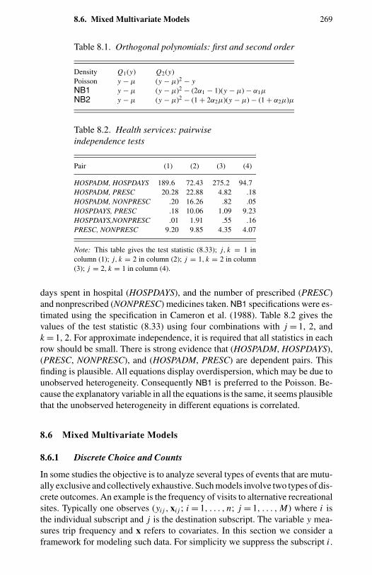
8.6. Mixed Multivariate Models 269

Table 8.1. Orthogonal polynomials: first and second order

Density Q1(y) Q2(y)Poisson y − µ (y − µ)2 − yNB1 y − µ (y − µ)2 − (2α1 − 1)(y − µ) − α1µ

NB2 y − µ (y − µ)2 − (1 + 2α2µ)(y − µ) − (1 + α2µ)µ

Table 8.2. Health services: pairwiseindependence tests

Pair (1) (2) (3) (4)

HOSPADM, HOSPDAYS 189.6 72.43 275.2 94.7HOSPADM, PRESC 20.28 22.88 4.82 .18HOSPADM, NONPRESC .20 16.26 .82 .05HOSPDAYS, PRESC .18 10.06 1.09 9.23HOSPDAYS,NONPRESC .01 1.91 .55 .16PRESC, NONPRESC 9.20 9.85 4.35 4.07

Note: This table gives the test statistic (8.33); j, k = 1 incolumn (1); j, k = 2 in column (2); j = 1, k = 2 in column(3); j = 2, k = 1 in column (4).

days spent in hospital (HOSPDAYS), and the number of prescribed (PRESC)and nonprescribed (NONPRESC) medicines taken. NB1 specifications were es-timated using the specification in Cameron et al. (1988). Table 8.2 gives thevalues of the test statistic (8.33) using four combinations with j = 1, 2, andk = 1, 2. For approximate independence, it is required that all statistics in eachrow should be small. There is strong evidence that (HOSPADM, HOSPDAYS),(PRESC, NONPRESC), and (HOSPADM, PRESC) are dependent pairs. Thisfinding is plausible. All equations display overdispersion, which may be due tounobserved heterogeneity. Consequently NB1 is preferred to the Poisson. Be-cause the explanatory variable in all the equations is the same, it seems plausiblethat the unobserved heterogeneity in different equations is correlated.

8.6 Mixed Multivariate Models

8.6.1 Discrete Choice and Counts

In some studies the objective is to analyze several types of events that are mutu-ally exclusive and collectively exhaustive. Such models involve two types of dis-crete outcomes. An example is the frequency of visits to alternative recreationalsites. Typically one observes (yi j , xi j ; i = 1, . . . , n; j = 1, . . . , M) where i isthe individual subscript and j is the destination subscript. The variable y mea-sures trip frequency and x refers to covariates. In this section we consider aframework for modeling such data. For simplicity we suppress the subscript i .

270 8. Multivariate Data

The starting point in such an analysis is to condition on the total number ofevents across all types, using the multinomial distribution,

f (y | N ) = N !

∏Mj=1 p

y j

j∏Mj=1 y j !

, (8.37)

where y = (y1, . . . ., yM ), y j ∈ 0, 1, 2, . . . ; j = 1, . . . , M where pj denotesthe probability of j th type of event, so that

∑p j = 1, y j denotes the frequency

of the j th event, and∑

y j = N denotes the total number of outcomes across thealternatives. The multinomial distribution is conditional on the total number ofall types of events, N . This is a useful specification for analyzing if N is given.

If it is assumed that each event frequency type has the Poisson density

f (y j = r j ) = e−µ j µr j

j

r j !, yj ∈ 0, 1, 2, . . . , j = 1, . . . , M,

then the frequencies of different events may be written as

f ∗(y1, . . . , yJ ) =M∏

j=1

e−µ j µr j

j

r j !. (8.38)

In this approach one simply estimates the Poisson regression for each type ofevent.

An alternative approach combines the conditional multinomial probabilitywith the probability of the total number of events,

Pr[y] = Pr[∑

y j = N]

Pr[y | N ],

where the probability function Pr[y | N ] is sometimes based on the multino-mial logit (Hausman, Leonard, and McFadden, 1995) or the conditional logit.Although in principle a more flexible specification such as the multinomial pro-bit may be used, the choice of the multinomial logit is computationally moretractable when M 3.

Terza and Wilson (1990) propose a mixed multinomial (logit) Poisson modelwhich is specified as

f MP(y) =(

M∏j=1

py j

j

)e−µµ

[∑Mj=1 y j

]∏M

j=1 y j !

,

where

p j = exp[x′

jβ j

]∑Mj=1 exp

[x′

jβ j

]µ =

M∑j=1

µ j ,

µ j = p jµ.

8.6. Mixed Multivariate Models 271

Combining these equations with the (8.38) specification, it is seen that themixed multinomial Poisson and the M individual Poisson specifications areequivalent.

The estimation of the mixed model by maximum likelihood is simplifiedon noting that the log-likelihood is additive in the parameters (β1, . . . ,βM )and µ. Hence, to maximize the likelihood one can sequentially estimate thesublikelihoods for the Poisson model for the total number of events, N , and forthe multinomial model for the choice probabilities, although not necessarily inthat order.

This analysis remains valid if the Poisson specification is replaced by one ofthe modified or generalized variants discussed in Chapter 4, and the multinomiallogit is replaced by a nested multinomial logit. For example, Terza and Wilson(1990) use a mixed multinomial logit and Poisson hurdles specification.

Hausman, Leonard, and McFadden (1995) develop a joint model of choiceof recreational sites and number of recreational trips. They use panel datafrom a large-scale telephone survey of Alaskan residents. Although there aresimilarities with Terza and Wilson (1990), their model explicitly incorporatesrestrictions from utility theory. The model conforms to a two-stage budgetingprocess. First a multinomial model is specified and estimated for explaining thechoice of recreational sites in Alaska. Explanatory variables x include the pricesassociated with the choice of sites. The estimates from this model are used toconstruct a price index for recreational trips. This price index subsequentlybecomes an explanatory variable in the count model for total number of trips,which the authors specify as a fixed-effects Poisson (see Chapter 9). The two-step modeling approach is described as utility consistent in the sense that it isconsistent with two-stage consumer budgeting. At step one the consuming unitallocates a utility-maximizing expenditure on the total number of trips. At thesecond stage this amount is optimally allocated across trips to alternative sites.

8.6.2 Counts and Continuous Variables

We begin with an example (van Praag and Vermeulen, 1993) in which thedata consist of number of events (shopping trips or number of plane trips),denoted by y1, and the vector of outcomes (recorded expenditures), denoted byy′

2 = (y21, . . . , y2k) where k refers to the number of events, y1 = k. The objectiveis to formulate a joint probability model

f (y1 |θ1)g(y2 |θ2, y1) = Pr[y1 = k] Pr[y′

2 = (y21, . . . , y2k)],

where (θ1,θ2) are unknown parameters, and x is a set of explanatory variables.In one formulation the joint modeling is accomplished by assuming that

conditional on x the variables y1 and y2 are stochastically independent. Onecould interpret this to mean that the dependency is captured through x. Underthis assumption the joint log-likelihood L(θ1,θ2) factors into a component forcount and another component for the amount, which may be estimated sepa-rately. The assumptions permit one to specify a flexible model for the counts,

272 8. Multivariate Data

accounting for example for the presence of excess of zero counts due to tastedifferences in the population, and possible truncation of expenditures due to,for example, expenditures smaller than a specified amount, say y2,min, not be-ing recorded. van Praag and Vermeulen (1993) estimate a count–amount modelfor tobacco, bakery, and aggregate food expenditures in which the frequenciesare modeled by a zero-inflated NB model and the amounts are modeled by atruncated normal.

The assumption of stochastic independence is convenient because it simpli-fies maximum likelihood estimation by making the log-likelihood functionallyseparable in the components θ1 and θ2, but in certain cases the assumptionmay be tenuous. For example, in the above case of the count–amount model,consider the availability of bulk discounts in shopping, which may provide anincentive for larger but fewer transactions. This dependency might be capturedby using bulk discount as an explanatory variable.

Maximum likelihood modeling of counts and amounts, or counts and otherdiscrete variables, allowing for stochastic dependencies, is problematic becauseof the obvious difficulty of formulating suitable joint probability distributions.In such cases moment-based estimators have a greater appeal.

8.7 Derivations

Kocherlakota and Kocherlakota (1993) show several ways in which the bivariatePoisson distribution may arise. The method of trivariate reduction is one that iscommonly used. The joint pgf of y1 and y2 defined at (8.6) and (8.7) is

P(z1, z2) = E[zy1

1 zy22

]= E

[zu

1 zv2(z1z2)w

]= exp[µ1(z1 − 1) + µ2(z2 − 1) + µ3(z1z2 − 1)]

= exp[(µ1 + µ3)(z1 − 1) + (µ2 + µ3)(z2 − 1)

+ µ3(z1 − 1)(z2 − 1)]. (8.39)

The marginal pgf are

Pj (z) = exp[(µ j + µ3

)(z − 1)], j = 1, 2, (8.40)

whence the marginal distributions are y1 ∼ P[µ1 + µ3] and y2 ∼ P[µ2 + µ3].The condition for the independence of y1 and y2 is that the joint pgf is theproduct of the two marginals, which is true iff µ3 = 0.

To derive the joint probability function expand (8.39) in powers of z1 and z2

as

P[z1, z2] = exp[µ1 + µ2 + µ3]∞∑

i=0

µi1zi

1

i!

∞∑j=0

µj2z j

2

j!

∞∑k=0

µk3zk

1zk2

k!,

(8.41)

8.8. Bibliographic Notes 273

which yields the joint frequency distribution as the coefficient of zr1zs

2:

f (y1 = r, y2 = s) = exp[µ1 + µ2 + µ3]min(r,s)∑

i=0

µr−i1 µs−i

2 µi3

(r − i)!(s − i)!i!.

(8.42)

The covariance between y1 and y2, using the independence of u, v, w, is givenby

Cov[y1, y2] = Cov[u + w, v + w]

= V[w]

= µ3,

and the correlation is given by

Cov[y1, y2]/√

V[y1] V[y2] = µ3/√

(µ1 + µ3)(µ2 + µ3).

Jung and Winkelmann (1993, pp. 555–556) provide first and second derivativesof the log-likelihood.

If the method of trivariate reduction is used, zero correlation between anypair implies independence.

8.8 Bibliographic Notes

An introductory survey of multivariate extensions of GLMs is given in Fahrmeierand Tutz (1994); see especially their treatment of multivariate models with cor-related responses. Formal statistical properties of bivariate discrete models arefound in Kocherlakota and Kocherlakota (1993) and Johnson, Kotz, and Bal-akrishnan (1997). Aitchison and Ho (1989) study a multivariate Poisson withlog-normal heterogeneity. Lindeboom and van den Berg (1994) analyze theimpact of heterogeneity on correlation between survival times in bivariate sur-vival models; their results are suggestive of consequences to be expected inbivariate count models. Arnold and Strauss (1988, 1992) and Moschopoulosand Staniswalis (1994) have considered the problem of estimating the param-eters of bivariate exponential family distributions with given conditionals. Theeconometric literature on estimation of multivariate models under conditionalmoment restrictions is relevant if the nonlinear generalized least squares orSPGLS approach is followed. But only some of this relates easily to countmodels; see Newey (1990a) and Chamberlain (1992a). Jung and Winkelmann(1993) consider the number of voluntary and involuntary job changes as abivariate Poisson process; Mayer and Chappell (1992) apply it to study deter-minants of entry and exit of firms. Bivariate count models have also been usedin sociology and political science. For example, Good and Pirog-Good (1989)consider several bivariate count models for teenage delinquency and paternity,but without the regression component. King (1989a) presented a bivariate model

274 8. Multivariate Data

of U.S. presidential vetoes of social welfare and defense policy legislation witha regression component. Meghir and Robin (1992) develop and estimate a jointmodel of frequency of purchase and a consumer demand system for eight typesof foodstuffs using French data on households that were observed to purchaseall eight foodstuffs over the survey period. They show that consistent estimationof the demand system may require data on frequency of purchase. They adopt asequential approach in which a frequency-of-purchase equation is estimated byNLS, and the ratio of the fitted mean to actual frequency of purchase is used toweight all observed expenditures. A system of demand equations is fitted usingthese reweighted expenditures.

CHAPTER 9

Longitudinal Data

9.1 Introduction

Longitudinal data or panel data are observations on a cross-section of individualunits such as persons, households, firms, and regions that are observed overseveral time periods. The data structure is similar to that of multivariate dataconsidered in Chapter 8. Analysis is simpler than for multivariate data becausefor each individual unit the same outcome variable is observed, rather thanseveral different outcome variables. Analysis is more complex because thissame outcome variable is observed at different points in time, introducing timeseries data considerations presented in Chapter 7.

In this chapter we consider longitudinal data analysis if the dependent vari-able is a count variable. Remarkably, many count regression applications are tolongitudinal data rather than simpler cross-section data. Econometrics exam-ples include the number of patents awarded to each of many individual firmsover several years, the number of accidents in each of several regions, and thenumber of days of absence for each of many persons over several years. Apolitical science example is the number of protests in each of several differ-ent countries over many years. A biological and health science example is thenumber of occurrences of a specific health event, such as seizure, for each ofmany patients in each of several time periods.

A key advantage of longitudinal data over cross-section data is that theypermit more general types of individual heterogeneity. Excellent motivationwas provided by Neyman (1965), who pointed out that panel data enable oneto control for heterogeneity and thereby distinguish between true and apparentcontagion. For example, consider estimating the impact of research and devel-opment expenditures on the number of patent applications by a firm, controllingfor individual firm-specific propensity to patent. For a single cross-section thesecontrols can only depend on observed firm-specific attributes such as industry,and estimates may be inconsistent if there is additionally an unobserved com-ponent to individual firm-specific propensity to patent. With longitudinal dataone can additionally include a firm-specific term for unobserved firm-specificpropensity to patent.

276 9. Longitudinal Data

The simplest longitudinal count data regression models are standard countmodels, with the addition of an individual specific term reflecting individualheterogeneity. In a fixed effects model this is a separate parameter for eachindividual. Creative estimation methods are needed if there are many individualsand hence parameters in the sample. In a random effects model this individualspecific term is instead drawn from a specified distribution. Then creativity isrequired either in choosing a distribution that leads to tractable analytical resultsor in obtaining estimates if results are not tractable.

Asymptotic theory requires that the number of observations, here the numberof individual units times the number of time periods, goes to infinity. We focuson the most common case of a short panel, in which only a few time periodsare observed and the number of cross-sectional units goes to infinity. We alsoconsider briefly the case in which the number of cross-sectional units is small butis observed for a large number of periods, as can be the case for cross-countrystudies. Then the earlier discussion for handling individual specific terms ismirrored in a similar discussion for time-specific effects. It is important torealize that the distribution of estimators, and which estimators are preferred,varies according to the type of sampling scheme.

In longitudinal data analysis the data are assumed to be independent overindividual units for a given year but are permitted to be correlated over timefor a given individual unit. In the simplest models this correlation over time isassumed to be adequately controlled for by individual-specific effects. In moregeneral models correlation over time is additionally introduced in ways similarto those used in time series analysis. Finally, as in time series models, one canconsider dynamic models or transition models that add a dynamic componentto the regression function, allowing the dependent variable this year to dependon its own value in previous years.

A review of the standard linear models for longitudinal data, with fixed ef-fects and random effects, is given in section 9.2, along with a statement of theanalogous models for count data. In section 9.3 fixed effects models for countdata are presented, along with application to data on the number of patentsawarded to each of 346 firms in each of the years 1975 through 1979. Randomeffects models are studied in section 9.4. In sections 9.3 and 9.4 both MLEsand moment-based estimators are detailed. A discussion of applications andof the relative merits of fixed effects and random effects approaches is givenin section 9.5. Model specification tests are presented in section 9.6. Dynamicmodels, in which the regressors include lagged dependent variables, are studiedin section 9.7.

9.2 Models for Longitudinal Data

In this chapter we consider almost exclusively models that include fixed orrandom individual-specific effects. Even simpler models ignore such effects,assuming that the variation in regressors across individuals is sufficient to cap-ture the differences in the dependent variable across individuals. We give little

9.2. Models for Longitudinal Data 277

attention to these simpler models, as they do not exploit the advantage of lon-gitudinal data over cross-section data.

9.2.1 Linear Models

Standard references for linear models for longitudinal data include Hsiao (1986),Diggle, Liang, and Zeger (1994), and Baltagi (1995). We give a brief review.

A quite general linear model for longitudinal data is

yit = αi t + x′i tβi t + uit , i = 1, . . . , n, t = 1, . . . , T, (9.1)

where yit is a scalar dependent variable, xi t is a k×1 vector of independent vari-ables and uit is a scalar disturbance term. The subscript i indexes an individualperson, firm, or country in a cross-section, and the subscript t indexes time. Thedistinguishing feature of longitudinal data models is that the intercept αi t andregressor coefficients βi t may differ across individuals or time. Such variationin coefficients reflects individual and time-specific effects. But the model (9.1)is too general and is not estimable. Further restrictions need to be placed on theextent to which αi t andβi t vary with i and t , and on the behavior of the error uit .

The simplest linear model is the one-way individual-specific effect model

yit = αi + x′i tβ + uit , i = 1, . . . , n, t = 1, . . . , T, (9.2)

where uit is iid with mean 0 and variance σ 2u . This is the standard linear re-

gression model, except that rather than one intercept α there are n individualspecific intercepts α1, . . . , αn . The two standard models based on (9.2) are thefixed effects linear model, which treats αi as a parameter to be estimated andexcludes an intercept from xi t , and the random effects linear model, whichtreats αi as an iid random variable with mean 0 and variance σ 2

α and includesan intercept in xi t .

For the fixed effects linear model the estimator of the slope coefficients is

βLFE =[

n∑i = 1

T∑t = 1

(xi t − xi )(xi t − xi )′]−1 n∑

i = 1

T∑t = 1

(xi t − xi )(yit − yi ),

(9.3)

where xi = 1T

∑Tt = 1 xi t and yi = 1

T

∑Tt = 1 yit are individual-specific averages

over time. The individual-specific fixed effects can be estimated by αi = yi −x′

i βLFE. For a short panel, that is, n → ∞ and T is fixed, βFE is consistent forβ, while αi is not consistent for αi as only T observations are used in estimatingeach αi .

The linear fixed effects estimator βLFE can be motivated in several ways.First, joint estimation of α and β in (9.2) by OLS yields (9.3) for β. Second,if εi t is assumed to be normally distributed, then (9.3) is obtained by maxi-mizing with respect to β the conditional likelihood function given

∑Tt = 1 yit ,

278 9. Longitudinal Data

i = 1, . . . , n, where∑T

t = 1 yit can be shown to be the sufficient statistic for αi .Third, (9.2) implies

(yit − yi ) = (xi t − xi )′β + (uit − ui ), (9.4)

meaning that differencing around the mean eliminates αi . The GLS estimatorof this equation can be shown to be OLS, and OLS of (yit − xi ) on (xi t − xi )yields (9.3). Using this interpretation βLFE is called the within estimator as itexplains variation in yit around yi by variation in xi t around xi – only variationwithin each individual is used.

For the random effects linear model the estimator of the slope coefficientestimator βLRE can be shown to be a matrix-weighted average of βLFE, definedin (9.3), and βLB obtained from the OLS regression

(yi − y) = (xi − x)′β + (ui − u),

where x = 1n

∑ni = 1 xi and y = 1

n

∑ni = 1 yi . The estimator βLB is called the be-

tween estimator as it uses only variation between individuals, essentially ig-noring the additional information available in a panel compared with a singlecross-section. The weights used to form βLRE from βLFE and βLB depend onthe variances σ 2

u and σ 2α . See basic treatments of this model.

The random effects estimator can be obtained in several ways. First, giventhe assumptions on the means and variances of uit and αi , it is the GLS estimatorfrom estimation of (9.2). Second, it is asymptotically equivalent to the MLE,which additionally assumes that uit and αi are normally distributed. The MLEin practice leads in small samples to different estimates of the variances σ 2

u andσ 2

α , and hence a different estimator of β, and is more difficult to estimate, as thelog-likelihood is nonlinear in the parameters. A third method, which providesbetter small-sample estimates of σ 2

u and σ 2α , is the restricted MLE method of

Patterson and Thompson (1971) and Harville (1977), reviewed in Diggle, Liang,and Zeger (1994, pp. 65–68).

The random and fixed effects linear models are compared by, for example,Hsiao (1986, pp. 41–47). The models are conceptually different, with the fixedeffects analysis being conditional on the effects for individuals in the sample;random effects is an unconditional or marginal analysis with respect to the pop-ulation. A major practical difference is that the fixed effects analysis providesonly estimates of time-varying regressors. Thus, for example, it does not allowestimation of an indicator variable for whether or not a patient in a clinical trialwas taking the drug under investigation (rather than a placebo). Another majordifference is that the random effects model assumption that individual effectsare iid implies that individual effects are uncorrelated with the regressors. If,instead, unobserved individual effects are correlated with observed effects, therandom effects estimator is inconsistent. Many econometrics studies in partic-ular prefer fixed effects estimators because of this potential problem.

Standard extensions to the linear model (9.2) are serial correlation in the error,for example, uit = ρuit−1 + εi t ; dynamic models, for example, xi t including

9.2. Models for Longitudinal Data 279

yi,t−1; and more general random effects models with random slope coefficientsin addition to random intercepts, for example, x′

i tβ is replaced by x′1i tβ1 +

x′2i tβ2i where β2i is iid with mean β2 and variance Σβ2 .

9.2.2 Count Models

For count models for longitudinal data, the starting point is the Poisson re-gression model with exponential mean function and multiplicative individualspecific term

yit ∼ P[µi t = αiλi t ]

λi t = exp(x′

i tβ), i = 1, . . . , n, t = 1, . . . , T .

(9.5)

Note that α used here refers to the individual effect and is not used in the sameway as in previous chapters, where it was an overdispersion parameter.

In the fixed effects model the αi are unknown parameters. Like the lin-ear model, estimation is possible by eliminating αi , either by conditioning on∑T

t = 1 yit , which requires fully parametric assumptions, or by using a quasi-differencing procedure that requires only first-moment assumptions.

In the random effects model the αi are instead iid random variables. As inthe linear model, estimation is possible either by assuming a distribution for αi

or by making second-moment assumptions, although unlike in the linear modelunder normality these can lead to quite different estimators.

A key departure from the linear model is that the individual specific effects in(9.5) are multiplicative, rather than additive as in the linear model (9.2). Giventhe exponential form for λi t , the multiplicative effects can still be interpretedas a shift in the intercept because

E[yit | xi t , αi ] = µi t

= αi exp(x′

i tβ)

= exp(δi + x′

i tβ), (9.6)

where δi = ln αi .Note that this equality between multiplicative effects and intercept shift does

not hold in some count data models, nor does it hold in noncount models such asbinary models to which similar longitudinal methods might be applied. Supposethe starting point is a more general conditional mean function g(x′

i tβ). Thensome models and estimation methods continue with multiplicative effects, so

E[yit | xi t , αi ] = µi t = αi g(x′

i tβ), (9.7)

while other methods use a shift in the intercept

E[yit | xi t , αi ] = µi t = g(δi + x′

i tβ). (9.8)

Results are most easily obtained for the Poisson. Extensions to the negativebinomial do not always work, and when they do work they do so for some

280 9. Longitudinal Data

methods for the NB1 model and in other cases for the NB2 model. It should bekept in mind, however, that a common reason for such extensions in using cross-section data is to control for unobserved heterogeneity. The longitudinal datamethods already control for heterogeneity, and Poisson longitudinal modelsmay be sufficient.

The following sections begin with fixed effects and random effects models,with no consideration to either serial correlation and dynamics. In particular,for multiplicative effects models the regressors xi t are initially assumed to bestrictly exogenous, so that

E[yit | xi1, . . . , xiT , αi ] = αiλi t . (9.9)

This is a stronger condition than E[yit | xi t , αi ] = αiλi t . This condition is relaxedwhen time series models are presented in section 9.7.

9.3 Fixed Effects Models

We consider three approaches to estimation of fixed effect count data models.First, we consider direct estimation by maximum likelihood, which may notnecessarily lead to consistent estimates for the common case in which T is fixedand n → ∞. Second, we present conditional maximum likelihood, which doesanalysis conditional on sufficient statistics for the individual effects. This worksfor NB1 models in addition to Poisson. Third, we consider a moment-basedapproach that bases estimation on a differencing transformation, which differsfrom that in the linear model, as here the effects are multiplicative, not additive.

9.3.1 Maximum Likelihood

The simplest fixed effects model for count data is the Poisson fixed effects model(9.5) where, conditional on λi t and parameters αi , yit is iid P[µi t = αiλi t ], λi t

is a specified function of xi t and β, and xi t excludes an intercept. At times wespecialize to the exponential form (9.6).

If n is small this model is easily estimated. In particular, the exponentialmean specification (9.6) can be rewritten as exp(

∑nj = 1 δ j d ji t + x′

i tβ), whered jit is an indicator variable equal to one if the i t th observation is for individualj and zero otherwise. Thus we can use standard Poisson software to regress yit

on d1i t , d2i t , . . . , dnit and xi t .This is impractical, however, if n is so large that (n + dim(β)) exceeds

software restrictions on the maximum number of regressors. In this chapterwe focus on the case in which n is large and T is small, in which case thisbarrier is likely to be encountered. Then analytical expressions for estimatorsof β and the αi are needed, analogous to those obtained for the linear model bypartitioning of the OLS estimator.

A potentially more serious problem is possible inconsistency of parameterestimates if T is small and n → ∞. This possibility arises because as n → ∞the number of parameters, n +dim(β), to be estimated goes to infinity, possibly

9.3. Fixed Effects Models 281

negating the benefit of a larger sample size, nT . The individual fixed effectscan be viewed as incidental parameters, because real interest lies in the slopecoefficients. For some fixed effects panel data models, too many incidentalparameters lead to inconsistent parameter estimates of β, in addition to αi . Aleading example is the logit model with fixed effects, with

Pr[yit = 1] = [αi + exp(x′

i tβ)]/[

1 + αi + exp(x′

i tβ)]

.

Hsiao (1986, section 7.3.1) demonstrates the inconsistency of the MLE for β inthis case, for fixed T and n → ∞. This inconsistency disappears, of course, ifT → ∞. In the case of the linear model, however, there is no such incidentalparameters problem.

An interesting question therefore is whether there is an incidental parametersproblem for the Poisson fixed effects model. The literature has generally notdirectly addressed this issue, although it has suggested that there is a problem.∗

For yit iid P[αiλi t ], the conditional joint density for the i th observation is

Pr [yi1, . . . , yiT | αi ,β]

=∏

t

[exp(−αiλi t ) (αiλi t )

yit/yit !]

= exp

(−αi

∑t

λi t

)∏t

αyit

i

∏t

λyit

i t

/∏t

yi t !. (9.10)

The corresponding log-density is

ln Pr [yi1, . . . , yiT | αi ,β] = −αi

∑t

λi t + ln αi

∑t

yi t

+∑

t

yi t ln λi t −∑

t

ln yit !.

Differentiating with respect to αi and setting to zero yields

αi =∑

t yi t∑t λi t

. (9.11)

Substituting this back into (9.10), simplifying and considering all n observationsyields the concentrated likelihood function,

Lconc(β) =∏

i

[exp

(−∑

t

yi t

)∏t

(∑t yi t∑t λi t

)yit ∏t

λyit

i t

/∏t

yi t !

]

∝∏

i

[∏t

(λi t∑s λis

)yit]

.

(9.12)

∗ We thank Frank Windmeijer and Tony Lancaster for pointing out that there is no incidentalparameters problem here. The proof given here is due to Tony Lancaster.

282 9. Longitudinal Data

This is the likelihood for n independent observations on a T -dimensional multi-nomial variable with cell probabilities

pit = λi t∑s λis

= exp(x′

i tβ)∑

s exp(x′

isβ) .

It follows that for the Poisson fixed effects model there is no incidentalparameters problem. Estimates of β that are consistent for fixed T and n →∞ can be obtained by maximization of ln Lconc(β) in (9.12). The first-orderconditions for this estimator are given in section 9.3.2, and its distribution isgiven in section 9.3.3 under much weaker conditions than those assumed here.Estimates of αi can then be obtained from (9.11) and are consistent if in factT → ∞.

This consistency of the MLE forβ despite the presence of incidental parame-ters is a special result that holds for the Poisson multiplicative fixed effects and,for continuous data, linear additive fixed effects. It holds in few other models,if any, in which case we need to transform the model into one in which the in-dividual effects do not appear. The next two subsections present different waysto do this. We begin with the simplest case, the Poisson, even though as alreadynoted there is no incidental parameters problem in this case.

9.3.2 Conditional Maximum Likelihood

The conditional maximum likelihood approach of Andersen (1970) performsinference conditional on the sufficient statistics for α1, . . . , αn , which for LEFdensities such as the Poisson are the individual-specific totals T yi = ∑T

t = 1 yit .In section 9.8.1 it is shown that for yit iid P[µi t ], the conditional joint densityfor the i th observation is

Pr

[yi1, . . . , yiT

∣∣∣∣ T∑t = 1

yit

]=(∑

t yi t)!∏

t yi t !×∏

t

(µi t∑s µis

)yit

. (9.13)

This is a multinomial distribution, with probabilities pit = µi t/∑

t µi t , t =1, . . . , T , which has already been used in section 8.6.

Models with multiplicative effects set µi t = αiλi t . This has the advantagethat simplification occurs as αi cancels in the ratio µi t/

∑s µis . Then (9.13)

becomes

Pr

[yi1, . . . , yiT

∣∣∣∣ T∑t = 1

yit

]=(∑

t yi t)!∏

t yi t !×∏

t

(λi t∑s λis

)yit

. (9.14)

Because yi1, . . . , yiT | ∑t yi t is multinomial distributed with probabilitiespi1, . . . , piT , where pit = λi t/

∑s λis, it follows that yit has mean pit

∑s yis .

Given (9.6) this implies that we are essentially estimating the fixed effects αi by∑s yis/

∑s λis .

9.3. Fixed Effects Models 283

In the special case λi t = exp(x′i tβ) this becomes

Pr

[yi1, . . . , yiT

∣∣∣∣ T∑t = 1

yit

]=(∑

t yi t)!∏

t yi t !×∏

t

(exp(x′

i tβ)∑

s exp(x′

isβ))yit

.

(9.15)

The conditional MLE of the Poisson fixed effects model βPFE therefore maxi-mizes the conditional log-likelihood function

Lc(β) =n∑

i = 1

[ln

(T∑

t = 1

yit

)! −

T∑t = 1

ln (yit !)

+T∑

t = 1

yit ln

(exp(x′

i tβ)∑T

s = 1 exp(x′

isβ))]. (9.16)

Note that this is proportional to the natural logarithm of Lconc(β) given in (9.12),and therefore here the concentrated MLE equals the MLE.

Differentiation of (9.16), or equivalently (9.12), with respect to β yieldsfirst-order conditions for βPFE that can be reexpressed as

n∑i = 1

T∑t = 1

xi t

(yit − λi t

yi

λi

)= 0, (9.17)

where yi = 1T

∑t yi t and λi = 1

T

∑t λi t and λi t = exp(x′

i tβ); see Blundell,Griffith, and Windmeijer (1995). The distribution of the resulting estimator canbe obtained using standard maximum likelihood theory. In practice it is betterto use results, given in the next subsection, obtained under weaker assumptionsthan yit iid P[αiλi t ].

The log-likelihood function (9.16) is similar to that of the multinomial logitmodel, except that yit is not restricted to taking only values zero or one and tosum over t to unity. Also the most standard form of a multinomial logit modelwith T outcomes has regressors fixed and parameters varying over the choices:pit = exp(x′

iβt )/∑T

s = 1 exp(x′iβs). Here instead the parameters β are constant

and the regressors xi t are time-varying.The Poisson fixed effects model was proposed by Palmgren (1981) and

Hausman, Hall, and Griliches (1984). The latter authors additionally presenteda negative binomial fixed effects model. Then yit is iid NB1 with parametersαiλi t and φi , where λi t = exp(x′

i tβ), so yit has mean αiλi t/φi and variance(αiλi t/φi ) ×(1 + αi/φi ).

This negative binomial model is of the less common NB1 form, with thevariance a multiple of the mean. The parameter αi is the individual-specificfixed effect; the parameter φi is the negative binomial overdispersion parame-ter, which is permitted to vary across individuals. Clearly αi and φi can onlybe identified to the ratio αi/φi , and even this ratio drops out for conditionalmaximum likelihood.

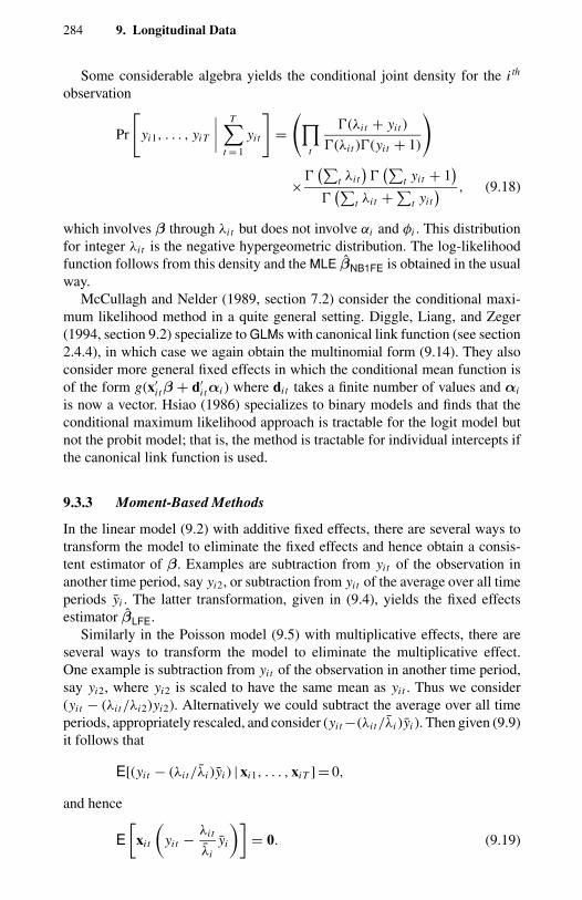
284 9. Longitudinal Data

Some considerable algebra yields the conditional joint density for the i th

observation

Pr

[yi1, . . . , yiT

∣∣∣∣ T∑t = 1

yit

]=(∏

t

(λi t + yit )

(λi t )(yit + 1)

)

×(∑

t λi t)(∑

t yi t + 1)

(∑

t λi t +∑t yi t) , (9.18)

which involves β through λi t but does not involve αi and φi . This distributionfor integer λi t is the negative hypergeometric distribution. The log-likelihoodfunction follows from this density and the MLE βNB1FE is obtained in the usualway.

McCullagh and Nelder (1989, section 7.2) consider the conditional maxi-mum likelihood method in a quite general setting. Diggle, Liang, and Zeger(1994, section 9.2) specialize to GLMs with canonical link function (see section2.4.4), in which case we again obtain the multinomial form (9.14). They alsoconsider more general fixed effects in which the conditional mean function isof the form g(x′

i tβ + d′i tαi ) where di t takes a finite number of values and αi

is now a vector. Hsiao (1986) specializes to binary models and finds that theconditional maximum likelihood approach is tractable for the logit model butnot the probit model; that is, the method is tractable for individual intercepts ifthe canonical link function is used.

9.3.3 Moment-Based Methods

In the linear model (9.2) with additive fixed effects, there are several ways totransform the model to eliminate the fixed effects and hence obtain a consis-tent estimator of β. Examples are subtraction from yit of the observation inanother time period, say yi2, or subtraction from yit of the average over all timeperiods yi . The latter transformation, given in (9.4), yields the fixed effectsestimator βLFE.

Similarly in the Poisson model (9.5) with multiplicative effects, there areseveral ways to transform the model to eliminate the multiplicative effect.One example is subtraction from yit of the observation in another time period,say yi2, where yi2 is scaled to have the same mean as yit . Thus we consider(yit − (λi t/λi2)yi2). Alternatively we could subtract the average over all timeperiods, appropriately rescaled, and consider (yit −(λi t/λi )yi ). Then given (9.9)it follows that

E[(yit − (λi t/λi )yi ) | xi1, . . . , xiT ] = 0,

and hence

E[

xi t

(yit − λi t

λiyi

)]= 0. (9.19)

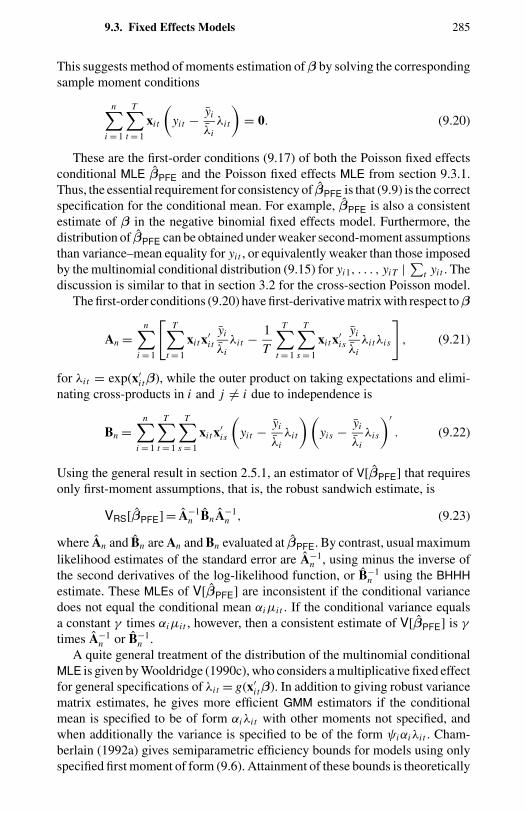
9.3. Fixed Effects Models 285

This suggests method of moments estimation ofβ by solving the correspondingsample moment conditions

n∑i = 1

T∑t = 1

xi t

(yit − yi

λiλi t

)= 0. (9.20)

These are the first-order conditions (9.17) of both the Poisson fixed effectsconditional MLE βPFE and the Poisson fixed effects MLE from section 9.3.1.Thus, the essential requirement for consistency of βPFE is that (9.9) is the correctspecification for the conditional mean. For example, βPFE is also a consistentestimate of β in the negative binomial fixed effects model. Furthermore, thedistribution of βPFE can be obtained under weaker second-moment assumptionsthan variance–mean equality for yit , or equivalently weaker than those imposedby the multinomial conditional distribution (9.15) for yi1, . . . , yiT | ∑t yi t . Thediscussion is similar to that in section 3.2 for the cross-section Poisson model.

The first-order conditions (9.20) have first-derivative matrix with respect toβ

An =n∑

i = 1

[T∑

t = 1

xi t x′i t

yi

λiλi t − 1

T

T∑t = 1

T∑s = 1

xi t x′is

yi

λiλi tλis

], (9.21)

for λi t = exp(x′i tβ), while the outer product on taking expectations and elimi-

nating cross-products in i and j = i due to independence is

Bn =n∑

i = 1

T∑t = 1

T∑s = 1

xi t x′is

(yit − yi

λiλi t

)(yis − yi

λiλis

)′. (9.22)

Using the general result in section 2.5.1, an estimator of V[βPFE] that requiresonly first-moment assumptions, that is, the robust sandwich estimate, is

VRS[βPFE] = A−1n BnA−1

n , (9.23)

where An and Bn are An and Bn evaluated at βPFE. By contrast, usual maximumlikelihood estimates of the standard error are A−1

n , using minus the inverse ofthe second derivatives of the log-likelihood function, or B−1

n using the BHHHestimate. These MLEs of V[βPFE] are inconsistent if the conditional variancedoes not equal the conditional mean αiµi t . If the conditional variance equalsa constant γ times αiµi t , however, then a consistent estimate of V[βPFE] is γ

times A−1n or B−1

n .A quite general treatment of the distribution of the multinomial conditional

MLE is given by Wooldridge (1990c), who considers a multiplicative fixed effectfor general specifications of λi t = g(x′

i tβ). In addition to giving robust variancematrix estimates, he gives more efficient GMM estimators if the conditionalmean is specified to be of form αiλi t with other moments not specified, andwhen additionally the variance is specified to be of the form ψiαiλi t . Cham-berlain (1992a) gives semiparametric efficiency bounds for models using onlyspecified first moment of form (9.6). Attainment of these bounds is theoretically

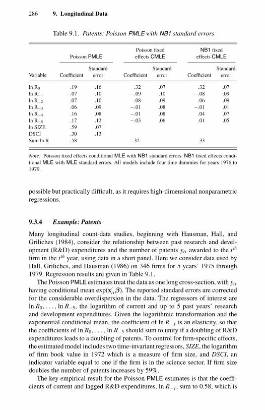
286 9. Longitudinal Data

Table 9.1. Patents: Poisson PMLE with NB1 standard errors

Poisson fixed NB1 fixedPoisson PMLE effects CMLE effects CMLE

Variable CoefficientStandard

error CoefficientStandard

error CoefficientStandard

error

ln R0 .19 .16 .32 .07 .32 .07ln R−1 −.07 .10 −.09 .10 −.08 .09ln R−2 .07 .10 .08 .09 .06 .09ln R−3 .06 .09 −.01 .08 −.01 .01ln R−4 .16 .08 −.01 .08 .04 .07ln R−5 .17 .12 −.03 .06 .01 .05ln SIZE .59 .07DSCI .30 .13Sum ln R .58 .32 .33

Note: Poisson fixed effects conditional MLE with NB1 standard errors. NB1 fixed effects condi-tional MLE with MLE standard errors. All models include four time dummies for years 1976 to1979.

possible but practically difficult, as it requires high-dimensional nonparametricregressions.

9.3.4 Example: Patents

Many longitudinal count-data studies, beginning with Hausman, Hall, andGriliches (1984), consider the relationship between past research and devel-opment (R&D) expenditures and the number of patents yit awarded to the i th

firm in the t th year, using data in a short panel. Here we consider data used byHall, Griliches, and Hausman (1986) on 346 firms for 5 years’ 1975 through1979. Regression results are given in Table 9.1.

The Poisson PMLE estimates treat the data as one long cross-section, with yit

having conditional mean exp(x′i tβ). The reported standard errors are corrected

for the considerable overdispersion in the data. The regressors of interest areln R0, . . . , ln R−5, the logarithm of current and up to 5 past years’ researchand development expenditures. Given the logarithmic transformation and theexponential conditional mean, the coefficient of ln R− j is an elasticity, so thatthe coefficients of ln R0, . . . , ln R−5 should sum to unity if a doubling of R&Dexpenditures leads to a doubling of patents. To control for firm-specific effects,the estimated model includes two time-invariant regressors, SIZE, the logarithmof firm book value in 1972 which is a measure of firm size, and DSCI, anindicator variable equal to one if the firm is in the science sector. If firm sizedoubles the number of patents increases by 59%.

The key empirical result for the Poisson PMLE estimates is that the coeffi-cients of current and lagged R&D expenditures, ln R− j , sum to 0.58, which is

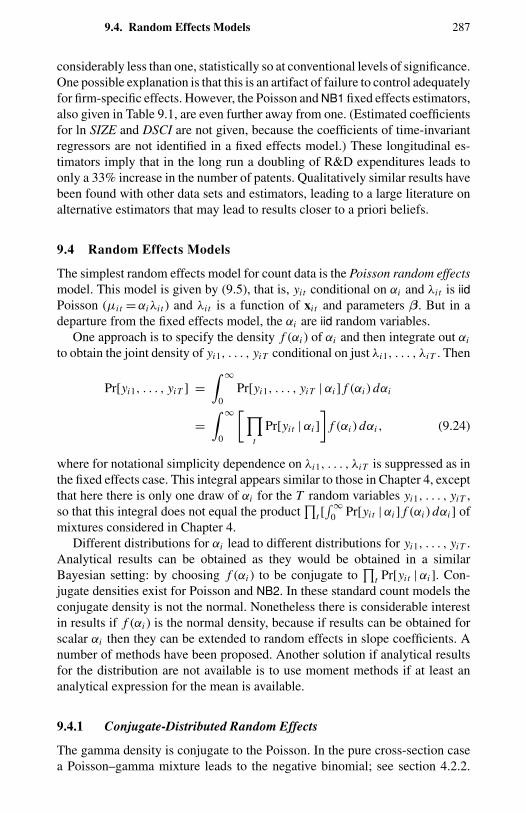
9.4. Random Effects Models 287

considerably less than one, statistically so at conventional levels of significance.One possible explanation is that this is an artifact of failure to control adequatelyfor firm-specific effects. However, the Poisson and NB1 fixed effects estimators,also given in Table 9.1, are even further away from one. (Estimated coefficientsfor ln SIZE and DSCI are not given, because the coefficients of time-invariantregressors are not identified in a fixed effects model.) These longitudinal es-timators imply that in the long run a doubling of R&D expenditures leads toonly a 33% increase in the number of patents. Qualitatively similar results havebeen found with other data sets and estimators, leading to a large literature onalternative estimators that may lead to results closer to a priori beliefs.

9.4 Random Effects Models

The simplest random effects model for count data is the Poisson random effectsmodel. This model is given by (9.5), that is, yit conditional on αi and λi t is iidPoisson (µi t = αiλi t ) and λi t is a function of xi t and parameters β. But in adeparture from the fixed effects model, the αi are iid random variables.

One approach is to specify the density f (αi ) of αi and then integrate out αi

to obtain the joint density of yi1, . . . , yiT conditional on just λi1, . . . , λiT . Then

Pr[yi1, . . . , yiT ] =∫ ∞

0Pr[yi1, . . . , yiT | αi ] f (αi ) dαi

=∫ ∞

0

[∏t

Pr[yit | αi ]

]f (αi ) dαi , (9.24)

where for notational simplicity dependence on λi1, . . . , λiT is suppressed as inthe fixed effects case. This integral appears similar to those in Chapter 4, exceptthat here there is only one draw of αi for the T random variables yi1, . . . , yiT ,so that this integral does not equal the product

∏t [∫∞

0 Pr[yit | αi ] f (αi ) dαi ] ofmixtures considered in Chapter 4.

Different distributions for αi lead to different distributions for yi1, . . . , yiT .Analytical results can be obtained as they would be obtained in a similarBayesian setting: by choosing f (αi ) to be conjugate to

∏t Pr[yit | αi ]. Con-

jugate densities exist for Poisson and NB2. In these standard count models theconjugate density is not the normal. Nonetheless there is considerable interestin results if f (αi ) is the normal density, because if results can be obtained forscalar αi then they can be extended to random effects in slope coefficients. Anumber of methods have been proposed. Another solution if analytical resultsfor the distribution are not available is to use moment methods if at least ananalytical expression for the mean is available.

9.4.1 Conjugate-Distributed Random Effects

The gamma density is conjugate to the Poisson. In the pure cross-section casea Poisson–gamma mixture leads to the negative binomial; see section 4.2.2.

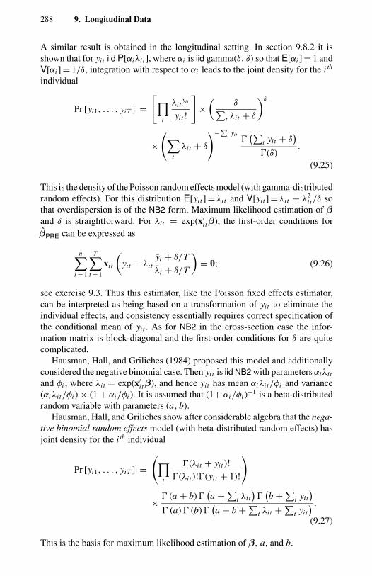
288 9. Longitudinal Data

A similar result is obtained in the longitudinal setting. In section 9.8.2 it isshown that for yit iid P[αiλi t ], where αi is iid gamma(δ, δ) so that E[αi ] = 1 andV[αi ] = 1/δ, integration with respect to αi leads to the joint density for the i th

individual

Pr [yi1, . . . , yiT ] =[∏

t

λi tyit

yi t !

]×(

δ∑t λi t + δ

)δ

×(∑

t

λi t + δ

)−∑t yi t(∑

t yi t + δ)

(δ).

(9.25)

This is the density of the Poisson random effects model (with gamma-distributedrandom effects). For this distribution E[yit ] = λi t and V[yit ] = λi t + λ2

i t/δ sothat overdispersion is of the NB2 form. Maximum likelihood estimation of βand δ is straightforward. For λi t = exp(x′

i tβ), the first-order conditions forβPRE can be expressed as

n∑i = 1

T∑t = 1

xi t

(yit − λi t

yi + δ/T

λi + δ/T

)= 0; (9.26)

see exercise 9.3. Thus this estimator, like the Poisson fixed effects estimator,can be interpreted as being based on a transformation of yit to eliminate theindividual effects, and consistency essentially requires correct specification ofthe conditional mean of yit . As for NB2 in the cross-section case the infor-mation matrix is block-diagonal and the first-order conditions for δ are quitecomplicated.

Hausman, Hall, and Griliches (1984) proposed this model and additionallyconsidered the negative binomial case. Then yit is iid NB2 with parameters αiλi t

and φi , where λi t = exp(x′i tβ), and hence yit has mean αiλi t/φi and variance

(αiλi t/φi ) × (1 + αi/φi ). It is assumed that (1+ αi/φi )−1 is a beta-distributedrandom variable with parameters (a, b).

Hausman, Hall, and Griliches show after considerable algebra that the nega-tive binomial random effects model (with beta-distributed random effects) hasjoint density for the i th individual

Pr [yi1, . . . , yiT ] =(∏

t

(λi t + yit )!

(λi t )!(yit + 1)!

)

× (a + b) (a +∑t λi t

)(b +∑t yi t

) (a) (b)

(a + b +∑t λi t +∑t yi t

) .(9.27)

This is the basis for maximum likelihood estimation of β, a, and b.

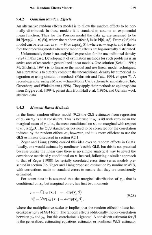
9.4. Random Effects Models 289

9.4.2 Gaussian Random Effects

An alternative random effects model is to allow the random effects to be nor-mally distributed. In these models it is standard to assume an exponentialmean function. Thus for the Poisson model the data yit are assumed to beiid P[exp(δi +x′

i tβ)], where the random effect δi is iid N[0, σ 2δ ]. From (9.6) this

model can be rewritten as yit ∼ P[αi exp(x′i tβ)], whereαi = exp δi , and is there-

fore the preceding model where the random effects are log-normally distributed.Unfortunately there is no analytical expression for the unconditional density

(9.24) in this case. Development of estimation methods for such problems is anactive area of research in generalized linear models. One solution (Schall, 1991;McGilchrist, 1994) is to linearize the model and use linear model techniques.An alternative is to directly compute the unconditional density by numerical in-tegration or using simulation methods (Fahrmeir and Tutz, 1994, chapter 7). Arecent example, using a Markov-chain Monte Carlo scheme to simulate, is Chib,Greenberg, and Winkelmann (1998). They apply their methods to epilepsy datafrom Diggle et al. (1994), patent data from Hall et al. (1986), and German workabsence data.

9.4.3 Moment-Based Methods

In the linear random effects model (9.2) the OLS estimator from regressionof yit on xi t is still consistent. This is because if αi is iid with zero mean themarginal mean of yit , i.e., the mean conditional on xi t but marginal with respectto αi , is x′

i tβ. The OLS standard errors need to be corrected for the correlationinduced by the random effects αi , however, and it is more efficient to use theGLS estimator discussed in section 9.2.1.

Zeger and Liang (1986) carried this idea over to random effects in GLMs.Ideally, one would estimate by nonlinear feasible GLS, but this is not practicalbecause unlike the linear case there is no simple analytical way to invert thecovariance matrix of y conditional on x. Instead, following a similar approachto that of Zeger (1988) for serially correlated error time series models pre-sented in section 7.6, Zeger and Liang proposed estimation by nonlinear WLS,with corrections made to standard errors to ensure that they are consistentlyestimated.

For count data it is assumed that the marginal distribution of yit , that isconditional on xi t but marginal on αi , has first two moments

µi t = E[yit | xi t ] = exp(x′

i tβ)

σ 2i t = Var[yit | xi t ] = φ exp

(x′

i tβ),

(9.28)

where the multiplicative scalar φ implies that the random effects induce het-eroskedasticity of NB1 form. The random effects additionally induce correlationbetween yit and yis , but this correlation is ignored. A consistent estimator for βis the generalized estimating equations estimator or nonlinear WLS estimator

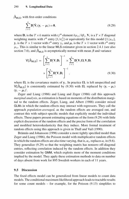
290 9. Longitudinal Data

βWLS, with first-order conditions

n∑i = 1

D′i Vi (yi − µi ) = 0, (9.29)

where Di is the T ×k matrix with t j th element ∂µi t/∂β j , Vi is a T ×T diagonalweighting matrix with t th entry [1/σ 2

i t ] or equivalently for this model [1/µi t ],yi is the T × 1 vector with t th entry yit and µi is the T × 1 vector with t th entryµi t . This is similar to the linear WLS estimator given in section 2.4.1 (see alsosection 7.6), and βWLS is asymptotically normal with mean β and variance

V[βWLS] =[

n∑i = 1

D′i Vi Di

]−1

×n∑

i = 1

D′i ViΩi Vi Di

×[

n∑i = 1

D′i Vi Di

]−1

, (9.30)

where Ωi is the covariance matrix of yi . In practice Ωi is left unspecified andV[βWLS] is consistently estimated by (9.30) with Ωi replaced by (yi −µi )(yi − µi )′.

Zeger and Liang (1986) and Liang and Zeger (1986) call this approachmarginal analysis, as estimation is based on moments of the distribution margi-nal to the random effects. Zeger, Liang, and Albert (1988) consider mixedGLMs in which the random effects may interact with regressors. They call theapproach population-averaged, as the random effects are averaged out, andcontrast this with subject-specific models that explicitly model the individualeffects. These papers present estimating equations of the form (9.29) with littleexplicit discussion of the random effects and the precise form of the correlationand modified heteroskedasticity that they induce. More formal treatment ofrandom effects using this approach is given in Thall and Vail (1990).

Brannas and Johansson (1996) consider a more tightly specified model thanZeger and Liang (1986), the Poisson model with multiplicative random effectsin which the random effects are also time varying, that is, αi t replaces αi in (9.6).They generalize (9.29) so that the weighting matrix has nonzero off-diagonalentries, reflecting correlation induced by the random effects. In addition theyconsider estimation by GMM, which exploits more of the moment conditionsimplied by the model. They apply these estimation methods to data on numberof days absent from work for 895 Swedish workers in each of 11 years.

9.5 Discussion

The fixed effects model can be generalized from linear models to count datamodels. The conditional maximum likelihood approach leads to tractable resultsfor some count models – for example, for the Poisson (9.13) simplifies to

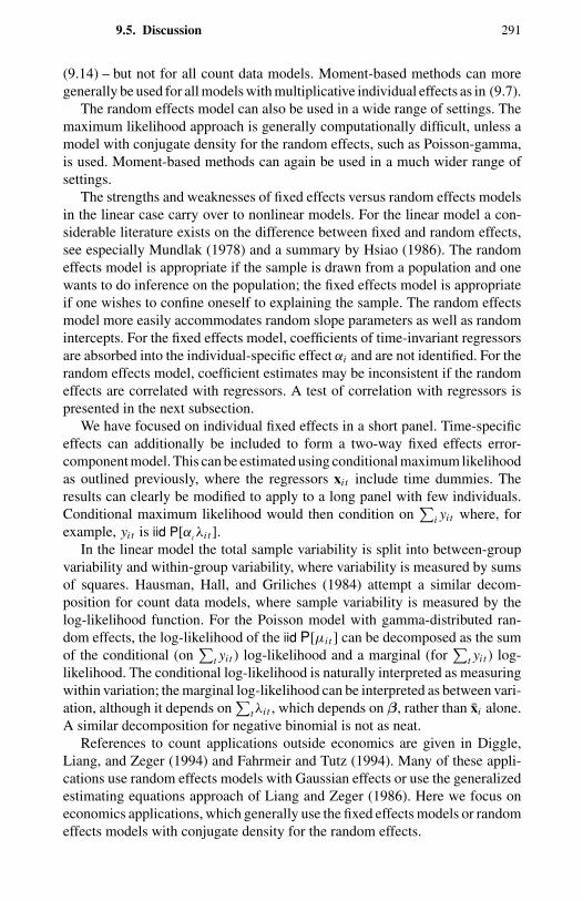
9.5. Discussion 291

(9.14) – but not for all count data models. Moment-based methods can moregenerally be used for all models with multiplicative individual effects as in (9.7).

The random effects model can also be used in a wide range of settings. Themaximum likelihood approach is generally computationally difficult, unless amodel with conjugate density for the random effects, such as Poisson-gamma,is used. Moment-based methods can again be used in a much wider range ofsettings.

The strengths and weaknesses of fixed effects versus random effects modelsin the linear case carry over to nonlinear models. For the linear model a con-siderable literature exists on the difference between fixed and random effects,see especially Mundlak (1978) and a summary by Hsiao (1986). The randomeffects model is appropriate if the sample is drawn from a population and onewants to do inference on the population; the fixed effects model is appropriateif one wishes to confine oneself to explaining the sample. The random effectsmodel more easily accommodates random slope parameters as well as randomintercepts. For the fixed effects model, coefficients of time-invariant regressorsare absorbed into the individual-specific effect αi and are not identified. For therandom effects model, coefficient estimates may be inconsistent if the randomeffects are correlated with regressors. A test of correlation with regressors ispresented in the next subsection.

We have focused on individual fixed effects in a short panel. Time-specificeffects can additionally be included to form a two-way fixed effects error-component model. This can be estimated using conditional maximum likelihoodas outlined previously, where the regressors xi t include time dummies. Theresults can clearly be modified to apply to a long panel with few individuals.Conditional maximum likelihood would then condition on

∑i yi t where, for

example, yit is iid P[αt λi t ].In the linear model the total sample variability is split into between-group

variability and within-group variability, where variability is measured by sumsof squares. Hausman, Hall, and Griliches (1984) attempt a similar decom-position for count data models, where sample variability is measured by thelog-likelihood function. For the Poisson model with gamma-distributed ran-dom effects, the log-likelihood of the iid P[µi t ] can be decomposed as the sumof the conditional (on

∑t yi t ) log-likelihood and a marginal (for

∑t yi t ) log-

likelihood. The conditional log-likelihood is naturally interpreted as measuringwithin variation; the marginal log-likelihood can be interpreted as between vari-ation, although it depends on

∑tλi t , which depends on β, rather than xi alone.

A similar decomposition for negative binomial is not as neat.References to count applications outside economics are given in Diggle,

Liang, and Zeger (1994) and Fahrmeir and Tutz (1994). Many of these appli-cations use random effects models with Gaussian effects or use the generalizedestimating equations approach of Liang and Zeger (1986). Here we focus oneconomics applications, which generally use the fixed effects models or randomeffects models with conjugate density for the random effects.

292 9. Longitudinal Data

The paper by Hausman, Hall, and Griliches (1984) includes a substantialapplication to number of patents for 121 U.S. firms observed from 1968 through1975. This paper estimates Poisson and NB models with both fixed and randomeffects. Other studies using patent data are discussed in section 9.7.

Ruser (1991) studies the number of workdays lost at 2788 manufacturingestablishments from 1979 through 1984. He uses the NB fixed effects estimatorand finds that workdays lost increase with higher workers’ compensation bene-fits, with most of the effect occurring in smaller establishments whose workers’compensation insurance premiums are less experience-rated.

Blonigen (1997) applies the NB2 random effects model to data on the numberof Japanese acquisitions in the United States across 365 three-digit StandardIndustry Classification industries from 1975 through 1992. The paper findsthat if the U.S. dollar is weak relative to the Japanese yen, Japanese acquisi-tions increase in industries more likely to involve firm-specific assets, notablyhigh R&D manufacturing sectors, which can generate a return in yen withoutinvolving a currency transaction.

In a novel application, Page (1995) applies the Poisson fixed effects modelto data on the number of housing units shown by housing agents to each oftwo paired auditors, where the two auditors are as much as possible identicalexcept that one auditor is from a minority group and the other is not. Specificallyblack/white pairs and Hispanic/Anglo pairs are considered. Here the subscript irefers to a specific auditor pair, i = 1, . . . , n; subscript t = 1, 2 refers to whetherthe auditor is minority (say t = 1) or nonminority (say t = 2). A simple modelwithout covariates is that E[yit ] = αi exp(βdit ), where dit = 1 if minority andequals 0 otherwise. Then exp(β) equals the ratio of population-mean housingunits shown to minority auditors to those shown to nonminority, and exp(β) < 1indicates discrimination is present. Page shows that in this case the Poissonfixed effects conditional MLE has explicit solution exp(β) = y1/y2. For the datastudied by Page (1995) exp(β) lies between 0.82 and 0.91, with robust standarderrors using (9.23) of between 0.022 and 0.028. Thus discrimination is present.Further analysis includes regressors that might explain the aggregate differencein number of housing units shown.

Van Duijn and Bockenholt (1995) analyze the number of spelling errors by721 first-grade pupils on each of four dictation tests. They consider a Poisson–gamma mixture model that leads to a conditional multinomial distribution. Thisdoes not adequately model overdispersion, so they consider a finite mixturesversion of this model using the methods of section 4.8. On the basis of chi-square goodness-of-fit tests they prefer a model with two classes, essentiallygood spellers and poor spellers.

Pinquet (1997) uses estimates of individual effects from longitudinal modelsof the number and severity of insurance claims to determine “bonus-malus”coefficients used in experience-rated insurance. In addition to an application toan unbalanced panel of over 100,000 policyholders, the paper gives considerablediscussion of discrimination between true and apparent contagion. A range ofmodels, including the random effects model of section 9.4, is considered.

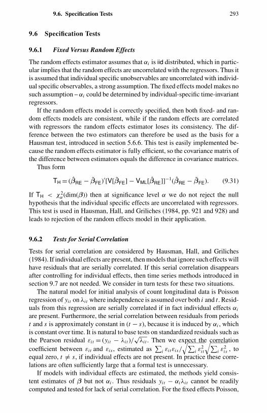
9.6. Specification Tests 293

9.6 Specification Tests

9.6.1 Fixed Versus Random Effects

The random effects estimator assumes that αi is iid distributed, which in partic-ular implies that the random effects are uncorrelated with the regressors. Thus itis assumed that individual specific unobservables are uncorrelated with individ-ual specific observables, a strong assumption. The fixed effects model makes nosuch assumption – αi could be determined by individual-specific time-invariantregressors.

If the random effects model is correctly specified, then both fixed- and ran-dom effects models are consistent, while if the random effects are correlatedwith regressors the random effects estimator loses its consistency. The dif-ference between the two estimators can therefore be used as the basis for aHausman test, introduced in section 5.6.6. This test is easily implemented be-cause the random effects estimator is fully efficient, so the covariance matrix ofthe difference between estimators equals the difference in covariance matrices.

Thus form

TH = (βRE − βFE)′[V[βFE] − VML[βRE]]−1(βRE − βFE). (9.31)

If TH < χ2α (dim(β)) then at significance level α we do not reject the null

hypothesis that the individual specific effects are uncorrelated with regressors.This test is used in Hausman, Hall, and Griliches (1984, pp. 921 and 928) andleads to rejection of the random effects model in their application.

9.6.2 Tests for Serial Correlation

Tests for serial correlation are considered by Hausman, Hall, and Griliches(1984). If individual effects are present, then models that ignore such effects willhave residuals that are serially correlated. If this serial correlation disappearsafter controlling for individual effects, then time series methods introduced insection 9.7 are not needed. We consider in turn tests for these two situations.

The natural model for initial analysis of count longitudinal data is Poissonregression of yit on λi t where independence is assumed over both i and t . Resid-uals from this regression are serially correlated if in fact individual effects αi

are present. Furthermore, the serial correlation between residuals from periodst and s is approximately constant in (t − s), because it is induced by αi , whichis constant over time. It is natural to base tests on standardized residuals such asthe Pearson residual εi t = (yit − λi t )/

√λi t . Then we expect the correlation

coefficient between εi t and εis , estimated as∑

i εi tεis/

√∑i ε2

i t

√∑i ε2

is , toequal zero, t = s, if individual effects are not present. In practice these corre-lations are often sufficiently large that a formal test is unnecessary.

If models with individual effects are estimated, the methods yield consis-tent estimates of β but not αi . Thus residuals yit − αiλi t cannot be readilycomputed and tested for lack of serial correlation. For the fixed effects Poisson,

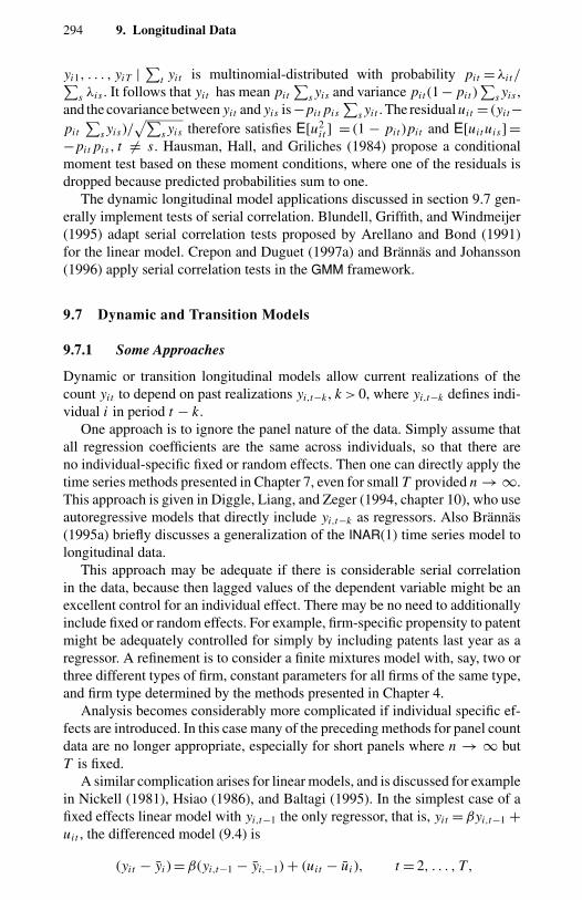
294 9. Longitudinal Data

yi1, . . . , yiT | ∑t yi t is multinomial-distributed with probability pit = λi t/∑s λis . It follows that yit has mean pit

∑s yis and variance pit (1 − pit )

∑s yis ,

and the covariance between yit and yis is−pit pis∑

s yit . The residual uit = (yit−pit∑

s yis)/√∑

s yis therefore satisfies E[u2i t ] = (1 − pit )pit and E[uit uis] =

−pit pis, t = s. Hausman, Hall, and Griliches (1984) propose a conditionalmoment test based on these moment conditions, where one of the residuals isdropped because predicted probabilities sum to one.

The dynamic longitudinal model applications discussed in section 9.7 gen-erally implement tests of serial correlation. Blundell, Griffith, and Windmeijer(1995) adapt serial correlation tests proposed by Arellano and Bond (1991)for the linear model. Crepon and Duguet (1997a) and Brannas and Johansson(1996) apply serial correlation tests in the GMM framework.

9.7 Dynamic and Transition Models

9.7.1 Some Approaches

Dynamic or transition longitudinal models allow current realizations of thecount yit to depend on past realizations yi,t−k , k > 0, where yi,t−k defines indi-vidual i in period t − k.

One approach is to ignore the panel nature of the data. Simply assume thatall regression coefficients are the same across individuals, so that there areno individual-specific fixed or random effects. Then one can directly apply thetime series methods presented in Chapter 7, even for small T provided n → ∞.This approach is given in Diggle, Liang, and Zeger (1994, chapter 10), who useautoregressive models that directly include yi,t−k as regressors. Also Brannas(1995a) briefly discusses a generalization of the INAR(1) time series model tolongitudinal data.

This approach may be adequate if there is considerable serial correlationin the data, because then lagged values of the dependent variable might be anexcellent control for an individual effect. There may be no need to additionallyinclude fixed or random effects. For example, firm-specific propensity to patentmight be adequately controlled for simply by including patents last year as aregressor. A refinement is to consider a finite mixtures model with, say, two orthree different types of firm, constant parameters for all firms of the same type,and firm type determined by the methods presented in Chapter 4.

Analysis becomes considerably more complicated if individual specific ef-fects are introduced. In this case many of the preceding methods for panel countdata are no longer appropriate, especially for short panels where n → ∞ butT is fixed.

A similar complication arises for linear models, and is discussed for examplein Nickell (1981), Hsiao (1986), and Baltagi (1995). In the simplest case of afixed effects linear model with yi,t−1 the only regressor, that is, yit = βyi,t−1 +uit , the differenced model (9.4) is

(yit − yi ) = β(yi,t−1 − yi,−1) + (uit − ui ), t = 2, . . . , T,

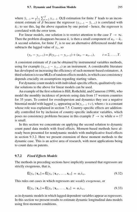
9.7. Dynamic and Transition Models 295

where yi,−1 = 1T −1

∑Tt = 2 yi,t−1. OLS estimation for finite T leads to an incon-

sistent estimate of β because the regressor (yi,t−1 − yi,−1) is correlated withui ; to see this, lag the above equation by one period – hence, the regressor iscorrelated with the error term.

For linear models, one solution is to restrict attention to the case T → ∞.Then the problem disappears because ui is then a small component of uit − ui .A second solution, for finite T , is to use an alternative differenced model thatsubtracts the lagged value of yit , so

(yit − yi,t−1) = β(yi,t−1 − yi,t−2) + (uit − uit−1), t = 2, . . . , T .

A consistent estimate of β can be obtained by instrumental variables methods,using for example (yi,t−2 − yi,t−3) as an instrument. A considerable literaturehas developed on increasing the efficiency of such moment-based estimators. Athird solution is to use MLEs of random effects models, in which case consistencydepends crucially on assumptions regarding starting values.

For dynamic count models with individual-specific effects, qualitatively sim-ilar solutions to the above for linear models can be used.

An example of the first solution is Hill, Rothchild, and Cameron (1998), whomodel the monthly incidence of protests using data from 17 western countriesfor 35 years. To control for overdispersion and dynamics they use a negativebinomial model with lagged yit appearing as ln(yi,t−1 +c), where c is a constantwhose role was explained in section 7.5. Country-specific effects are addition-ally controlled for by inclusion of country-specific indicator variables, whichposes no consistency problems because in this example T → ∞ while n = 17is small.

In this section we concentrate on applying the second solution to dynamiccount panel data models with fixed effects. Moment-based methods have al-ready been presented for nondynamic models with multiplicative fixed effectsin section 9.3.2. Here we present extension of these moment methods to thedynamic case. This is an active area of research, with most applications beingto count data on patents.

9.7.2 Fixed Effects Models

The methods in preceding sections have implicitly assumed that regressors arestrictly exogenous, that is,

E[yit | xi t ] = E[yit | xiT , . . . , xi1] = αiλi t . (9.32)

This rules out cases in which regressors are weakly exogenous, or

E[yit | xi t ] = E[yit | xi t , . . . , xi1] = αiλi t , (9.33)

as in dynamic models in which lagged dependent variables appear as regressors.In this section we present results to estimate dynamic longitudinal data modelsusing first-moment conditions.

296 9. Longitudinal Data

We begin by considering the Poisson fixed effects estimator introduced insection 9.3. Given independence over i , the first-order conditions for β givenin (9.17) have expected value zero if

E

[T∑

t = 1

xi t

(yit − yi

λiλi t

)]= 0. (9.34)

The presence of the average yi , introduced to eliminate the fixed effects, inthese moment conditions limits application of this estimator to strictly ex-ogenous regressors. To see this, consider the t th term in the sum and assumeE[yit | xi1, . . . , xiT ] = αiλi t as in (9.32). Then E[yi | xi1, . . . , xiT ] = αi λi and

E[

xi t

(yit − yi

λiλi t

)]= Exi1,...,xiT

[xi tE

[yit − yi

λiλi t | xi1, . . . , xiT

]]= Exi1,...,xiT

[xi t

(αiλi t − αi λi

λiλi t

)]= 0.

Note that it is not enough to assume E[yit | xi t ] = αiλi t , because this doesnot necessarily imply E[yi | xi t ] = αi λi . For example, suppose xi t = yit−1 andE[yit | yit−1] = αiρyit−1, or λi t = ρyit−1. Then

E [yi | yit−1] = E[

1

T(yi1 + · · · + yiT ) | yit−1

]while

αi λi = 1

Tαiρ(yi0 + · · · + yiT −1).

Equality of the two requires E[yis | yit−1] = αiρyis−1 for s = t , which is clearlynot the case. Similar problems arise if we assume E[yit | xi t , . . . , xi1] = αiλi t ,because again this does not imply E[yi | xi t , . . . , xi1] = αi λi .

One could instead eliminate fixed effects by quasidifferencing, as noted atthe beginning of section 9.3.2. For weakly exogenous regressors, Chamberlain(1992b) proposes eliminating the fixed effects by the transformation

qit = yit − λi t

λi t+1yit+1. (9.35)

Suppose instruments zi t exist such that

E[yit − αiλi t | zi t , . . . , zi1] = 0. (9.36)

Then

E[yit+1 − αiλi t+1 | zi t , . . . , zi1]

= Ezi t+1 [E[yit+1 − αiλi t+1 | zi t+1, zi t , . . . , zi1]]

= Ezi t+1 [0]

= 0.

9.7. Dynamic and Transition Models 297

It follows that

E[

yit − λi t

λi t + 1yit + 1 | zi t , . . . , zi1

]= αiλi t − λi t

λi t+1αiλi t+1

= 0.

In the case in which there are as many instruments as parameters one solves

T∑t = 1

zi t

(yit − λi t

λisyis

)= 0. (9.37)

As an example, suppose

E[yit | yit−1, . . . , xi t , . . .] = αiλi t = αi(ρyit−1 + exp

(x′

i tβ))

.

Then the natural choice of instruments is zi t = (yit−1, xi t ).If there are more instruments zi t than regressors, such as through adding ad-

ditional lags of regressors into the instrument set, one can consistently estimateβ by the GMM estimator, which minimizes

1

n

(n∑

i = 1

qi (β)′zi

)W−1

n

(n∑

i = 1

z′i qi (β)

), (9.38)

where qi (β) = (qi1 · · · qiT )′, zi = (z′i1 · · · z′

iT

)′, W−1

n is a weighting matrix, and,given specification of qi and zi , the optimal choice of Wn is Wn = ∑n

i = 1 z′i qi

q′i zi where qi = qi (β) and β is an initial consistent estimate obtained for ex-

ample by minimizing (9.38) with Wn = In .An alternative transformation to eliminate the fixed effects is

qit = yit

λi t− yit + 1

λi t + 1, (9.39)

proposed by Wooldridge (1997), which is simply the earlier choice divided byλi t . Yet another possibility is the mean scaling transformation

qit = yit − yi0

λi0λi t , (9.40)

proposed by Blundell, Griffith, and Windmeijer (1995), where yi0 is the pre-sample mean value of yi and the instruments are (xi t −xi0). The latter estimatorleads to estimates that are inconsistent, but in a simulation this inconsistency isshown to be small, and efficiency is considerably improved. This estimator isespecially useful if data on the dependent variable go back farther in time thandata on the explanatory variables.

These methods are applicable to quite general models with multiplicativefixed effects. Several studies, beginning with Montalvo (1997), have refined andapplied these methods, mostly to count data on patents. Application to patentsis of particular interest for several reasons. There are few ways to measureinnovation aside from patents, which are intrinsically a count. R&D expendi-tures affect patents with a considerable lag, so there is potentially parsimony

298 9. Longitudinal Data

and elimination of multicollinearity in having patents depend on lagged patentsrather than a long-distributed lag in R&D expenditures. And, as noted in theexample earlier, most studies using distributed lags on R&D expenditure findthe R&D expenditure elasticity of patents to be much less than unity.

Blundell, Griffith, and Windmeijer (1995) model the U.S. patents data ofHall, Griliches, and Hausman (1986). They pay particular attention to the func-tional form for dynamics and the time series implications of various functionalforms. The lagged dependent variable is introduced in either multiplicativefashion as

µi t = αi exp(ρ ln y∗

i t − 1 + x′i tβ)

where y∗i t − 1 = yit − 1 unless yit − 1 = 0 in which case y∗

i t − 1 = c, or additive fash-ion as

µi t = ρyit − 1 + αi exp(x′

i tβ),

where ρ > 0. Another variant of the additive model, not considered, is

µi t = αi(ρyit − 1 + exp

(x′

i tβ))

.

In their application up to two lags of patents and three lags of R&D expendituresappear as regressors. The estimates indicate long lags in the response of patentsto R&D expenditures.

Related studies by Blundell, Griffith, and Van Reenen (1995a, b) model thenumber of “technologically significant and commercially important” innova-tions commercialized by British firms. Dynamics are introduced more simply byincluding the lagged value of the knowledge stock, an exponentially weightedsum of past innovations.

Montalvo (1997) uses the Chamberlain (1992b) transformation to model thenumber of licensing agreements by individual Japanese firms and the Hall et al.(1986) data. Lagged dependent variables do not appear as regressors. InsteadMontalvo argues that current R&D expenditures cannot be assumed to be strictlyexogenous because patents depend on additional R&D expenditures for theirfull development. So there is still a need for quasidifferenced estimators.

Crepon and Duguet (1997a) apply GMM methods to French patents data.They also use a relatively simple functional form for dynamics. First, as regres-sor they use a measure of R&D capital. This capital measure is calculated asthe weighted sum of current and past depreciated R&D expenditure and canbe viewed as imposing constraints on R&D coefficients in a distributed lagmodel. Dynamics in patents are introduced by including indicator variables forwhether yit−1 is in the ranges 1 to 5, 6 to 10, or 11 or more. Particular attentionis paid to model specification testing and the impact of increasing the size ofthe instrument set zi in (9.38).

In a more applied study, Cincera (1997) includes not only a distributed lagin firm R&D expenditures but also a distributed lag in R&D expenditures byother firms in the same sector to capture spillover effects. Application is to apanel of 181 manufacturing firms from six countries.

9.8. Derivations 299

9.8 Derivations

9.8.1 Conditional Density for Poisson Fixed Effects

Consider the conditional joint density for observations in all time periods for agiven individual, where for simplicity the individual subscript i is dropped. Ingeneral the density of y1, . . . , yT given

∑t yt is

Pr

[y1, . . . , yT

∣∣∣∣ ∑t

yt

]= Pr

[y1, . . . , yT ,

∑t

yt

]/Pr

[∑t

yt

]

= Pr [y1, . . . , yT ]

/Pr

[∑t

yt

],

where the last equality arises because knowledge of∑

t yt adds nothing givenknowledge of y1, . . . , yT .

Now specialize to yt iid Poisson (µt ). Then Pr[y1, . . . , yT ] is the product ofT Poisson densities, and

∑t yt is Poisson (

∑t µt ). It follows that

Pr

[y1, . . . , yT

∣∣∣∣ ∑t

yt

]=

∏t

(exp(−µt )µ

ytt /yt !

)exp(−∑t µt

)(∑t µt)∑

t yt/(∑

t yt)!

= exp(−∑t µt

)∏t µ

ytt

/∏t yt !

exp(−∑t µt

)∏t

(∑s µs)yt/(∑

t yt)!

=(∑

t yt)!∏

t yt !×∏

t

(µt∑s µs

)yt

.

Introducing the subscript i yields (9.13) for Pr [yi1, . . . , yiT | ∑t yi t ].

9.8.2 Density for Poisson with Gamma Random Effects

Consider the joint density for observations in all time periods for a given indi-vidual, where for simplicity the individual subscript i is dropped. From (9.13)the joint density of y1, . . . , yT if yt | α is P[αλt ] is

Pr[y1, . . . , yT ] =∫ ∞

0

[∏t

(e−αλt (αλt )

yt /yt !)]

f (α) dα

=∫ ∞

0

[∏t

λytt /yt !

](e−α

∑t λt · α

∑t yt)

f (α) dα

=[∏

t

λytt /yt !

]×∫ ∞

0

(e−α

∑t λt · α

∑t yt)

f (α) dα.

Now let f (α) be the gamma density with parameters density. Similar algebra tothat in section 4.2.2 yields the Poisson random effects density given in (9.25).

300 9. Longitudinal Data

9.9 Bibliographic Notes

Longitudinal data models fall in the class of multilevel models, surveyed byGoldstein (1995), who includes a brief treatment of Poisson. Standard refer-ences for linear models for longitudinal data include Hsiao (1986), Diggle,Liang, and Zeger (1994), and Baltagi (1995). Diggle et al. (1994) and Fahrmeirand Tutz (1994) consider generalized linear models in detail. A useful referencefor general nonlinear longitudinal data models is Matyas and Sevestre (1995).

There are remarkably many different approaches to nonlinear models, andmany complications including serial correlation, dynamics and unbalanced pan-els. The treatment here is comprehensive for models used in econometrics andcovers many of the approaches used in other areas of statistics. Additionalstatistical references can be found in Diggle et al. (1994) and Fahrmeir andTutz (1994). Lawless (1995) considers both duration and count models for lon-gitudinal data for recurrent events. For dynamic models the GMM fixed effectsapproach is particularly promising. In addition to the count references given insection 9.7, it is useful to refer to earlier work for the linear model by Arellanoand Bond (1991) and Keane and Runkle (1992).

9.10 Exercises

9.1 Show that the Poisson fixed effects conditional MLE of β that maximizesthe log-likelihood function given in (9.16) is the solution to the first-orderconditions (9.17).

9.2 Find the first-order conditions for the negative binomial fixed effects con-ditional MLE of β that maximizes the log-likelihood function based on thedensity (9.18). (Hint: Use the gamma recursion as in section 3.3.) Do thesefirst-order conditions have a simple interpretation, like those for the Poissonfixed effect conditional MLE?

9.3 Verify that the first-order conditions for the Poisson random effects MLEfor β can be expressed as (9.26).

9.4 Show that the Poisson fixed effects conditional MLE that solves (9.17)reduces to exp(β) = y1/y2 in the application by Page (1995) discussed at theend of section 9.5.

CHAPTER 10

Measurement Errors

10.1 Introduction

The well-known bivariate linear errors-in-variables regression model with addi-tive measurement errors in both variables provides one benchmark for nonlinearerrors-in-variables models. The standard textbook treatment of the errors-in-variables case emphasizes the attenuation result, which says that the estimatedleast squares estimate of the slope parameter is downward-biased if both vari-ables are subject to measurement error. The essential problem lies in the correla-tion between the observed explanatory variable and the measurement error. Thisleads to distorted inferences about the role of the covariate. Although this resultdoes not always extend to general cases, such as a linear model with two or morecovariates measured with error, it is usually of interest to consider whether a sim-ilar attenuation bias exists generally in nonlinear models (Carroll et al., 1995).

There are important similarities and differences between measurement errorsin nonlinear and linear models. First, in nonlinear models it may be more naturalto allow measurement errors to enter multiplicatively rather than additively.Second, models in which the measurement errors are confined to the countvariable, rather than covariates, are of considerable interest. Third, the directionof measurement errors in count models is sometimes strongly suspected froma priori analysis, which permits stronger conclusions.

Given these motivations, this chapter considers estimation and inference inthe presence of measurement errors in exposure time, errors due to underreport-ing and misclassification of events. Such errors are shown to have importantconsequences for model identification, specification, estimation, and testing.One way to analyze the impact of measurement errors is to consider whatimpact they have on the properties of a particular estimator that might be oth-erwise optimal. We also emphasize the effect of the measurement error on theobserved distribution of counts, and the consequences of the choice of modelingapproaches for such data.

A general approach is to introduce measurement errors in the counts andthe covariates, together with assumptions about the joint distribution of errors.Although this case is of major interest, we shall begin with a slightly simpler

302 10. Measurement Errors

case in which the measurement error affects only the count variable. We thenfocus on its effect on the distribution of the response variable.

We follow this discussion with an analysis of measurement errors in thecovariates, without being specific about their origin. In an important class ofcases, measurement errors are shown to lead to overdispersion.

There are two other cases in which the appropriate method of inference isof special interest. In the first case, we are interested in event counts that areunderreported. For example, certain types of crime, accidents, and absencesat the place of work may be underreported because of random failures in themechanism for recording those events. How should estimation and inferencebe carried out in such cases?

There is a closely related second case if one is interested in the frequency dis-tribution of a subset of several related types of events, for example, the frequencyof industrial accidents in some particular category. However, the events may beoccasionally misclassified, sometimes because of lack of clarity in the definitionof the event, and sometimes to understate the relative frequency of one type ofevent. Whittemore and Gong (1991) analyze data on cervical cancer mortalityrates using mortality data for several European countries coded into interna-tional classification of disease categories. They point out that there are severalpotential sources of error and systematic intercountry differences in the desig-nation of the code, leading to misclassification errors. As in the case of underre-ported counts, the main interest is in various approaches to modeling such data.

Section 10.2 examines the impact of measurement errors in counts due tothe incorrectly measured exposure. The emphasis is on overdispersion. Sec-tion 10.3 concentrates on the case of additive or multiplicative measurementerrors in the regressors, ignoring the errors in counts. Section 10.4 studiesmeasurement errors in counts that do not necessarily arise from mismeasuredexposure, including the practically important case of misclassified counts. Sec-tion 10.5 analyzes estimation and inference for underreported counts, whicharise in many commonly occurring situations.

10.2 Measurement Errors in Exposure

It useful to distinguish between separate measurement errors in exposure (periodof occurrence) and intensity (rate of occurrence). For example, in analyzing thenumber of insurance claims for auto accidents, an error arises if it is assumedthat all cases in the sample were covered by insurance for the whole of theperiod under study, if in truth some members were only covered for some partof the period. This is an example of measurement error in exposure. Suppose themodel calls for a variable reflecting driving experience, but the only measureavailable is the number of years a driving license has been held, which is animperfect measure of driving experience. This is an example of measurementerror in the intensity component. These are considered first.

Let us begin with the initial specification of the Poisson density in Chapter 1

f (yi | µi ti ) = e−µi ti (µi ti )yi

yi !, yi = 0, 1, . . . . (10.1)

10.2. Measurement Errors in Exposure 303

Compactly, we refer to this density as P[µi ti ]. This is written to emphasizethe distinction between the intensity parameter µi and the exposure period ti ,defined as the period during which the subject is at “risk” of experiencing theevent. Under the assumption that the exposure period is correctly measuredand of unit length for all subjects, E[yi ] = µi ti = µi . Then the density may bewritten without the exposure period, thus f (yi | µi ) = exp(−µi )µ

yi

i /yi !.Again we assume µi = µ(xi ,β) for convenience. It is of interest to consider

the consequences of measurement errors for the MLE. Measurement errors inyi , xi , and ti are relevant, those in xi for obvious reasons and those in ti becauseit is a likely source of measurement error in cases in which the sample dataare based on the subject’s possibly faulty recall of events experienced in thepast. Exposure need not necessarily be just time, because other variables suchas population, distance, and so forth may also be relevant. Measurement errorsfrom exposures in the general case have been considered by Brannas (1996)and Alcaniz (1996).

In analyzing the consequences of measurement errors one may either fo-cus on the properties of a particular estimator, such as inconsistency, or studythe effect on the entire distribution of the observed random variable. The firstapproach is widely used in the analysis of linear errors-in-variables models.The main technique in the latter case involves considering a small-variancelocal Taylor expansion around the true density (Cox, 1983) and studying theproperties of the resulting approximate density.

In relation to exposures, three separate cases are considered. The first isthe case of known but unequal exposures, which can be handled in a relativelystraightforward manner. The second situation is that in which the exposure vari-able is not directly observed but there is information on observable factors thataffect it. The third case is one in which the exposure period is not observed andis incorrectly assumed to be the same for all subjects, giving rise to measure-ment errors. A potential advantage of specifying exposure explicitly is to permitseparate identification of factors that affect exposure rather than the intensityparameter.

10.2.1 Correctly Observed Exposure

Using the exponential mean specification we have

µi ti = exp(x′

iβ)ti

= exp(x′

iβ + ln ti)

= exp

[(x′

i ln ti) (β

1

)]= exp

[x′

iβ(a)], (10.2)

where x′i = (xi ln ti ) and β(a)′ = (β′ βk+1) = (β′ 1). With this specification

substituted in the usual expression for log-likelihood, estimation can proceed via

304 10. Measurement Errors

constrained maximum likelihood, with the coefficient of ln ti being restricted tounity. This constraint can be imposed directly by substitution into the likelihood.Another alternative is to estimate βk+1 freely and then use the test of the nullhypothesis that βk+1 = 1 as a model specification test.

10.2.2 Multiplicative Error in Exposure

In this section we show that a measurement error in exposure is analogous toa measurement error in the dependent variable in the linear regression. A con-sequence is to inflate the variance through overdispersion. Under appropriateassumptions we find strong parallels between measurement errors and unob-served heterogeneity. Both lead to overdispersion, and in both cases, providedthere is no dependence with explanatory variables, maximum likelihood is aconsistent estimator. There are also strong parallels in the algebraic analysis ofthe two problems.

Assume that µi (·) is correctly specified, but ti is measured with error. Alsoassume that the measurement error is uncorrelated with the explanatory vari-ables xi . Suppose the model is estimated by Poisson maximum likelihood.

In considering the impact of measurement error on the properties of theestimator, notice that the model set-up is exactly analogous to the case of mul-tiplicative heterogeneity considered in earlier chapters. The variable ti replacesthe term νi . Consequently, in the presence of random measurement errors in ti ,the mixed Poisson model emerges. If ti is gamma-distributed, for example, theresulting marginal distribution of yi is the NB2. Formally, we have

f (yi | µi ti ) = µyi

i

yi !

t yi

i

eµi ti

= P[µi ] × e−ti t yi

i . (10.3)

To handle the problem without an explicit parametric assumption regarding thedistribution of ti , we follow the approach of Gurmu, Rilstone, and Stern (1995):

h(yi | µi ) =∫

f (yi | µi , ti )g(ti ) dti

= µyi

i

yi !

∫t yi

i e−(µi ti )g(ti ) dti

= µyi

i

yi !M(y)

t (−µi ), (10.4)

where Mt (−µi ) = Et [e−µi ti ] denotes the moment generating function for ti and

M(y)t (−µi ) = Et

[t yi

i e−(µi ti )]

(10.5)

is the ythi order derivative of Mt (−µi ) with respect to −µi ; Et denotes ex-

pectation with respect to the mixing distribution. Essentially (10.4) gives the

10.2. Measurement Errors in Exposure 305

arbitrary, and hence flexible, mixed Poisson density, which can be analyzedafter choosing a suitable g(t) density and then doing the necessary algebra toderive the term M(y)

t (−µi ). Although this approach is quite general, it generatesformidable algebraic and computational detail, as shown in section 12.5.

Continuing with the assumption that the intensity function µ(·) is correctlyspecified, the assumption of a multiplicative measurement error with a spec-ified parametric distribution leads to a mixed (overdispersed) Poisson model.Interestingly, this implies that overdispersion in a count model may reflectmeasurement errors. For example, the assumption that ti in (10.3) has gammadistribution leads to the marginal distribution of yi being the negative binomialdistribution.

We say the measurement errors are exogenous if they are uncorrelated withthe covariates xi . Under the assumption of exogenous measurement errors, itfollows that the random measurement errors in exposures do not affect theconsistency property of the Poisson maximum likelihood. Furthermore, if thevariance of the measurement errors is O(n−1/2) (a case of “modest overdisper-sion” in Cox’s [1983] terminology), then the estimator is also asymptoticallyefficient. A heuristic demonstration of this point follows from a second-orderTaylor expansion of (10.1) around (ti − 1). In general, however, the standarderrors of the PML estimator will be incorrect and should be adjusted.

First it is assumed that the true exposure period is of unit length, and themeasurement error, ti − 1, is zero mean, finite variance, and uncorrelated withyi − µi :

Et [ti − 1] = 0,

Et [(ti − 1)(yi − µi )] = 0,

Et [(ti − 1)2] = σ 2i .

(10.6)

The second-order Taylor expansion around P[µi ] yields

e−µi ti (µi ti )yi

yi != P[µi ]

[1 + (yi − µi )(ti − 1)

+ 1

2((yi − µi )

2 − yi )(ti − 1)2 + O(ti − 1)3].

Then

Et

[e−µi ti (µi ti )yi

yi !

]≈ P[µi ]

[1 + 1

2((yi − µi )

2 − yi )σ2i

]/a(µi , σ

2i

)(10.7)

where a(µi , σ2i ) is a normalizing constant.

From (10.7) it can be seen that, under the assumption that measurement er-rors are O(n−1/2), the neglect of overdispersion is not asymptotically a seriousmisspecification, although it affects the estimates of the sample covariance ma-trix of β. We can also interpret this result to mean that the use of mixed Poisson

306 10. Measurement Errors

models may be justified by the presence of particular types of measurementerrors.

Suppose (yi − µi ) and (ti − 1) are correlated, and

Et [(yi − µi )(ti − 1)] ≡ σi (xi , ti ).

Then

Et

[e−µi ti (µi ti )yi

yi !

]≈ P[µi ]

[1 + σi (xi , ti ) + σ 2

i

2[(yi − µi )

2 − yi ]

]/a(µi , σ

2i

).

Unlike the previous case, the moments of this distribution depend on the distri-bution of ti through the covariance σi (xi , ti ). Consequently, as the first momentof the distribution is no longer µi , estimators based on the Poisson mean spec-ification will be inconsistent. In general, the entire distribution of yi , not justthe variance, is affected by this type of measurement error. Heuristically, theinclusion in the conditional mean function of variables correlated with ti shouldreduce the extent of misspecification. This provides a motivation for using proxyvariables for exposure.

10.2.3 Proxy Variables for Exposure

In some cases the exposure is more realistically specified as a function of a setof observables. For example, Dionne, Desjardins, Laberque-Nadeau, and Maag(1995) estimate the effect of different medical conditions on truck drivers’distribution of accidents, including exposure factors measured by hours behindthe wheel, kilometers driven, and other qualitative factors. The conditional meanfunction is specified as a function of variables that affect the intensity of theprocess (x1) and those that affect the exposure (x2); thus

µi ti | x1i , x2i = exp(x′

1iβ1 + ln ti)

= exp

[(x′

1i x′2i

) (β1

β2

)],

(10.8)

which does not require constrained estimation. A random error may also beincluded in the conditional mean. For example, if

ti = exp(x′

2iβ2)ui ,

where u denotes an error with unit mean, then one will get results similar tothose in the previous subsection.

10.3. Measurement Errors in Regressors 307

10.3 Measurement Errors in Regressors

10.3.1 Additive Measurement Errors

Some data sets have two features. First, the assumption that covariates aremeasured with additive Gaussian errors is reasonable. Second, one has accessto replicated data sets that make it feasible to estimate moments of the errordistribution. In such cases the approach of Carroll et al. (1995) may be applied.

Consider the case in which the true regressors X in the conditional meanfunction are not observed, but a proxy, W, where W = X + U, is observed; theadditive measurement error U is assumed to be distributed N[0,Σuu]. The anal-ysis is based on the conditional distribution of Y given the error-contaminatedvariable W, although the main interest is in the conditional distribution of Ygiven X. Carroll et al. propose two “functional methods” for generalized linearmodels, which, unlike “structural methods,” make minimal assumptions aboutthe distribution of regressors. The analysis is specialized to the Poisson regres-sion. They suggest two methods, the “conditional-score” and the “corrected-score” methods. The first step in applying these methods is to obtain an estimateof the sufficient statistic for X. The standard estimating equations for the Pois-son model can then be modified by replacing the term in the score functioninvolving X by the sufficient statistic. Assuming that an estimate of Σuu isavailable, the adjusted estimating equations still cannot be written in a closedform for the Poisson regression; summation of an infinite series is necessary.Second, estimation of Σuu requires additional data; this step may be feasibleif replicates of W are available, which may be the case in some disciplines.Finally, the calculation of sampling variances is implemented using bootstrap-type methods. In short, this method of dealing with measurement errors is quitecomputer-intensive. For further details the reader is referred to the originalsources. Jordan, Brubacher, Tsugane, Tsubono, Gey, and Moser (1997) con-sider a similar model that does not require replicated data. Their estimationprocedure is Bayesian and simulation-based.

The analysis does not shed any direct light on the existence of attenuationbias. A heuristic qualitative argument suggests that a downward bias is ex-pected. Measurement errors in covariates increase the range of variation of theexplanatory variables without a corresponding effect on the range of the re-sponse variable. Consequently unit variation in W elicits a smaller responsethan unit variation in X. The quantitative impact of attenuation can be expectedto vary depending on the nonlinearity of the conditional mean.

10.3.2 Multiplicative Error in Regressors

In this subsection we consider the case of multiplicative measurement errors.With the exponential specification for the conditional mean, the multiplicativeerror model, the additive error model, and the unobserved heterogeneity modelscan be shown to be algebraically similar. Hence, under certain assumptions

308 10. Measurement Errors

some of the effects of additive or multiplicative errors turn out to be verysimilar. Different implications can be generated, however, by changes in thoseassumptions.

Consider the exponential mean model with multiplicative heterogeneity.Specifically, let

yi | µi , νi ∼ P[µiνi ],

where

µiνi = exp(x′

iβ)νi

= exp(x′

iβ+ εi), (10.9)

where exp(εi ) = νi .Now let us compare this with the additive measurement error model in which

yi | µi ∼ P[µi ],

where

µi = exp(x∗′

i β), (10.10)

where x∗ is the vector of unobserved true values of explanatory variables.Assume that x∗ = x + η, which has an additive measurement error η, so that

E[yi | xi ,ηi ] = exp[(xi + ηi )′β]

= exp(x′

iβ)exp(η′

iβ)

= exp(x′

iβ)wi , (10.11)

where wi = exp(η′iβ). This formulation has an obvious parallel with unob-

served heterogeneity. Clearly one might interpret the unobserved heterogeneityterm in (10.9) as a measurement error. One may also interpret it as reflectingomitted regressors z as in

µi | xi , zi = exp(x′

iβ + z′iγ)

= exp(x′

iβ)exp(z′

iγ)

= exp(x′

iβ)ui , (10.12)

where ui = exp(z′iγ), which is again algebraically similar to the preceding

measurement error and heterogeneity models.These similarities can be exploited by reinterpreting the analysis of the pre-

vious subsection. For example, parallel to (10.6), we may specify

Ew[wi − 1] = 0; Ew[(wi − 1)2] = σ 2w,i ;

Ew[(wi − 1)(yi − µi )] ≡ σi (xi , wi ).

10.4. Measurement Errors in Counts 309

Further, parallel to (10.7) we can derive

Ew

[e−µi wi (µiwi )yi

yi !

]

≈ P[µi ]

[1 + σi (xi , wi ) + σ 2

w,i

2[(yi − µi )

2 − yi ]

]/a(µi , σ

2w,i

).

So the effects of additive measurement are qualitatively similar to those dueto omitted heterogeneity, errors in exposure, or omitted regressors from theconditional mean. If the measurement errors are uncorrelated with the regressorsx, then E[η | x] = E[η] and wi has unit mean and finite variance. Then theconsequences of measurement error are essentially the same as those due tounobserved heterogeneity, namely overdispersion and loss of efficiency of thePML estimator.

An alternative assumption allows for possible correlation between x and η.Mullahy (1997a) has argued by reference to the omitted variable case thatnonzero correlation is more realistic. That is, one or more of the omitted regres-sors are likely to be correlated with the included variables. Then the standardPMLE is also inconsistent.

Under certain assumptions, the nonlinear instrumental variable estimatorprovides consistent estimates of the parameters of the model. Write the modelin matrix notation as a nonlinear regression,

y = exp(Xβ) + ε, (10.13)

where it is assumed that E[ε | X] = 0, V[ε | X] = Ω. Assume that we haveavailable wi , a set of g, g ≥ k+m instrumental variables that are asymptoticallyuncorrelated with εi and correlated with xi . The set of instruments may includea subset of xi . The NLIV estimator, denoted βNLIV, minimizes

(y − exp(Xβ))′W(W′ΩW)−1W′(y − exp(Xβ)),

for a given Ω. Two points to note are that the nonlinear regression has anadditive, not multiplicative, error, and that the specification and estimationof the (optimal) weighting matrix Ω should be considered. These issues arediscussed again in Chapter 11.

10.4 Measurement Errors in Counts

10.4.1 Additive Measurement Errors in Counts

Suppose that error-contaminated counts, denoted by yo, are nonnegative andinteger-valued. Let yt denote the true unobserved count and ε the additivemeasurement error. That is,

yo = yt + ε, yt , ε 0. (10.14)

310 10. Measurement Errors

One simple model is

yt | µ ∼ P[µ]

ε | γ ∼ P[γ ],

and yt and ε are independently distributed. This implies that

yo | µ, γ ∼ P[µ + γ ].

So the measurement error leads to a larger mean and variance relative to thedistribution of yt . This model has a nonnegative measurement error; hence, itis useful only for characterizing count inflation.

More generally we might consider the case where ε is integer-valued but notnecessarily nonnegative. This assumption permits both under- and overcounts.But the nonnegativity restriction on yo implies parallel restrictions on the distri-bution of ε. It is implausible to expect such restrictions to hold if it is assumedthat yt and ε are independently distributed. A joint distribution for yt and ε,which admits correlation, may seem more appropriate. The distribution of yo

may be derived by adding a joint distribution to (10.14).Binomial thinning, considered in section 7.4, is another example of a mech-

anism for modeling measurement errors in counts. This mechanism operatessuch that an event that has occurred is not recorded. Such nonrecording thenoccurs a random number of times and only affects events, not nonevents. How-ever, as its name suggests, this mechanism generates only undercounts – henceits usefulness in modeling underreporting. Binomial thinning is the opposite ofthe model of count inflation suggested previously. It is used in section 10.5 tomodel underreported counts.

One may construct a synthetic model that accommodates both under- andovercounts. An example is a finite mixture involving two “pure” types of con-tamination, one generating only positive and the other generating only negativemeasurement error. Currently such models remain underdeveloped.

10.4.2 Misclassified Counts

Counted events may be categorized by types. Classification into types may itselfbe subject to error, leading to incorrect total number of events in each category.The basic idea of this subsection is that improvements result from modeling theclassification process. This intuitive idea also recurs in section 10.5, in whichwe consider underrecording.

We shall begin with an example based on Whittemore and Gong (1991), whoconsider a situation in which the main interest lies in the mortality rate fromcervical cancer using cross-country grouped data on deaths and population atrisk in different age groups. We change their notation slightly to be consistentwith previous notation in this chapter. They assume that the disease may bemisclassified as one of several other diseases but that its diagnosis is unlikely to

10.4. Measurement Errors in Counts 311

be erroneous. That is, “Process of classifying has perfect specificity, but imper-fect sensitivity denoted by π , and the sensitivity π may vary with covariates”(Whittemore and Gong, 1991, p. 83).

Denote by n1i and n2i the number of correct and incorrect disease classifica-tions, respectively; i = 1, . . . , G. Assume (i) n1i ∼ B(πi , n1i +n2i ); (ii) diseaseoccurs in each population as a Poisson process; and (iii) distinct populationsare independent.

Then the Poisson assumption about actual occurrence of the disease im-plies that observed fallible disease counts ys

i are mutually independent Poissonvariates. That is,

ysi ∼ P

[µc

i

]µc

i = πiµi

= πiλi Li ,

where µi denotes the disease rate and Li denotes person-years at risk. BecauseLi is known, the focus is on modeling the disease rate λi . The likelihood forthe i th observation is then the product of Poisson and binomial likelihoods

Li = (µci

)ysi e−µc

i πn1,i

i (1 − πi )n2,i/

ysi !

and the log-likelihood is

L(λ, π | X, Ys, L, Z, n1, n2) =G∑

i = 1

ys

i ln πi + ysi ln λi − πiλi Li

+ n1,i ln πi + n2,i ln(1 − πi ),

(10.15)

where in what follows λi = exp(x′iβ), and

πi = exp(z′

iδ)/[1 + exp

(z′

iδ)]=

(z′

iδ),

which allows the covariates in λ and π terms to differ in principle. Let dim(xi ) =k, dim(zi ) = s. This specification is slightly different from Whittemore andGong’s example in which exactly the same covariates determine both λi andπi . The likelihood scores are:

∂L∂β

=∑(

ysi − µc

i

)xi

∂L∂δ

=∑((

ysi − µc

i

)(1 −

(z′

iδ))+ n1i − (n1i + n2i )

(z′

iδ))

zi ,

(10.16)

where the second block of s equations can be interpreted as implying orthog-onality between the covariates zi and the difference between the actual and

312 10. Measurement Errors

expected frequency of disease counts, allowing for misclassification probabil-ity. The (k + s)-dimensional information matrix is given by

I(β, δ) =n∑

i=1

[µc

i xi x′i Iβδ

I ′βδ µc

i (1 − (ziδ))zi z′i

], (10.17)

where

Iβδ =∑[

n1i + n2i + µi(1 −

(z′

iδ))][

(z′

iδ)(1 − (ziδ))

]x′

i zi .

Note that unless the subsets of covariates x and z are mutually orthogonal,the information matrix is not block-diagonal. As before, for identifiability werequire that rank [I(β, δ)] is k + s.

The example discussed above is closely related to the work on log-linearmodels for categorical data with misclassification errors. There are some simi-larities between this approach and that used in the underrecorded counts prob-lem, especially in relation to modeling the misclassification probability in termsof observed covariates. However, binomial thinning plays a role in underrecord-ing, but not here. Hence, the frequency of observations within the categorymay be under- or overreported. If one is interested in more than two misclas-sification categories, a multinomial logit model offers a suitable parameteri-zation. For other possible generalizations, see Whittemore and Gong (1991,pp. 90–91).

10.4.3 Outlying Counts

Let us reconsider the data set on recreational trips that was used in Chapter 6.There was a suspicion of measurement errors in this case arising from thecurious “rounding” in the number of self-reported boating trips if that numberwas 10 or higher (see Table 6.9). Some clustering occurs at 10 and 15 trips, andhigher counts often occur in rounded categories like 20, 25, 30, 40, and 50.

To avoid distorted inferences from such data, robust estimation based ondiscarding some proportion of the data is sometimes recommended. However,Christmann (1994, 1996) notes that the finite sample breakdown points of manyrobust estimators for regressions with discrete responses are not known. He con-siders the least median of weighted squares estimator for the Poisson regressionand shows that it has a high breakdown point and other desirable properties.

More informally, in practice it may be useful to simply form an impressionof the impact of the high counts on the estimated model. One way to do this isto “downweight” the higher counts in which we believe the measurement errormight be concentrated. For example, we might truncate the sample at 10 visitsif we believe that for frequencies larger than this value the measurement erroris too large. Then we might estimate a truncated negative binomial model using10 visits as a truncation point. Another possibility is to use 10, or some othervalue, as the censoring point in estimating the right censored negative binomial.This procedure also reduces the weight of large frequencies but less drastically

10.5. Underreported Counts 313

than in the truncated case. A limitation of this idea is that it only explores theconsequences of suspected measurement errors and lacks formal justification.For example, how should one choose among different censoring values? Therobust estimation approach addresses this problem more formally.

10.5 Underreported Counts

In this section we consider how one might model event counts if there is reasonto believe that some events that have occurred might not be recorded. It is easyto see that if events are distributed with mean µ, and each event has a constantprobability π of being observed, then the observed event count has mean πµ.So a count model fitted to observed data yields information about the productπµ. This is clearly a downward-biased estimate of µ, the true mean of the eventprocess. This section considers refinements of this model using the basic ideathat modeling the recording process may result in improved inference aboutparameters of interest.

10.5.1 Mechanism and Examples

The term underrecording refers to that feature of the method of data collectionthat causes the observed (recorded) count to understate on average the actualnumber of events. Parametric estimation and inference are to be based on therecorded counts of the event.

Suppose events are generated by a pure count process, but for each event, aBernoulli process determines whether the event is recorded. This is the bino-mial thinning mechanism. For a given recording probability for an individualevent, the occurrence probability may be either dependent or independent. Ineither case, the recorded events are shown to follow a mixed binary process.A regression model can be developed by parameterizing the moments of themixed process. The main idea is to combine a model of underrecording with amodel of the count process.

Examples of underrecorded counts may be found in many fields. Theyinclude the frequency of absenteeism in workplaces (Barmby, Orme, andTreble, 1991; Johansson and Palme, 1996), the reporting of industrial injuries(Ruser, 1991), the number of violations of safety regulations in nuclear powerplants (Feinstein, 1989, 1990), the frequency of criminal victimization (Fien-berg, 1981; Schneider, 1981; Yannaros, 1993), hospital medicine (Watermann,Jankowski, and Madan, 1994), and earthquakes and cyclones (Solow, 1993), tomention only a few.

The example of absenteeism in the workplace serves to illustrate certainrecurring features of underreported-count models. In some organizations therecorded absences at work reflect the interaction between the actual incidenceof absenteeism and the monitoring mechanism for observing those absences.Monitoring mechanisms are usually not perfect because such observation re-quires resources, whose use may not be economical beyond a certain point,

314 10. Measurement Errors

which itself can be expected to vary across organizations. Let y denote the truenumber of events. Suppose the probability that an event is recorded, conditionalon occurrence, is π , 0 ≤ π ≤ 1. Assume that the recording and occurrencemechanisms are independent. Then the mean number of recorded events, de-noted ys , is

E[ys | µ, π ] = µπ,

where E[y | µ] = µ is the true mean and π is the average recording probability.This argument suggests a simple nonlinear regression approach to estimationbased on parameterizing theµ andπ components. If, for example,µ = µ(x,β),and π = π (z,γ), where µ(·) and π (·) are known functions, the approach leadsto a nonlinear regression of the form

ys = µ(x,β)π (z,γ) + ε. (10.18)

If (β,γ) are identifiable, then a consistent estimation procedure may be devised.If not, then one may estimate a “reduced form” – type regression

ys = m(x, z |θ) + ε, (10.19)

where m(·) may be a given function and θ is some (generally unknown) func-tion of (β,γ). In the subsequent discussion, we take (10.18) as the equationof interest. Although this basic framework is useful in approaching the prob-lem, we begin by considering the more general case in which there is depen-dence between observation and recording. However, irrespective of whetherthe two are dependent, the key idea is that recording should be modeled, notignored.

10.5.2 Dependence Between Events and Recording

Consider a bivariate binomial random variable (Y, R) where Y = 1 denotes thesingle occurrence of an event of interest in some specified time interval, andR = 1 denotes the recording of that event. The following table establishes thenotation for the probabilities associated with the four possible outcomes:

R = 1 R = 0Y = 1 π11 π10 π

Y = 0 π01 π00 1 − π

π ′ 1 − π ′

The recording process is not directly observable. It is assumed that whereasan event that has occurred may not be recorded (observed), the nonoccurrenceof an event is always correctly recorded. Thus, there is zero probability ofoverrecording.

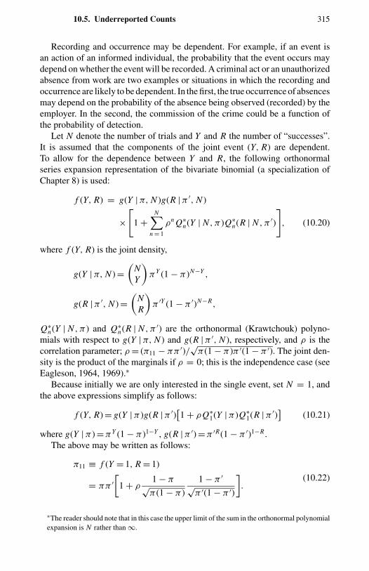
10.5. Underreported Counts 315

Recording and occurrence may be dependent. For example, if an event isan action of an informed individual, the probability that the event occurs maydepend on whether the event will be recorded. A criminal act or an unauthorizedabsence from work are two examples or situations in which the recording andoccurrence are likely to be dependent. In the first, the true occurrence of absencesmay depend on the probability of the absence being observed (recorded) by theemployer. In the second, the commission of the crime could be a function ofthe probability of detection.

Let N denote the number of trials and Y and R the number of “successes”.It is assumed that the components of the joint event (Y, R) are dependent.To allow for the dependence between Y and R, the following orthonormalseries expansion representation of the bivariate binomial (a specialization ofChapter 8) is used:

f (Y, R) = g(Y | π, N )g(R | π ′, N )

×[

1 +N∑

n = 1

ρn Q∗n(Y | N , π )Q∗

n(R | N , π ′)

], (10.20)

where f (Y, R) is the joint density,

g(Y | π, N ) =(

NY

)πY (1 − π )N−Y ,

g(R | π ′, N ) =(

NR

)π ′Y (1 − π ′)N−R,

Q∗n(Y | N , π ) and Q∗

n(R | N , π ′) are the orthonormal (Krawtchouk) polyno-mials with respect to g(Y | π, N ) and g(R | π ′, N ), respectively, and ρ is thecorrelation parameter; ρ = (π11 − ππ ′)/

√π (1 − π )π ′(1 − π ′). The joint den-

sity is the product of the marginals if ρ = 0; this is the independence case (seeEagleson, 1964, 1969).∗

Because initially we are only interested in the single event, set N = 1, andthe above expressions simplify as follows:

f (Y, R) = g(Y | π )g(R | π ′)[1 + ρQ∗

1(Y | π )Q∗1(R | π ′)

](10.21)

where g(Y | π ) = πY (1 − π )1−Y , g(R | π ′) = π ′R(1 − π ′)1−R .The above may be written as follows:

π11 ≡ f (Y = 1, R = 1)

= ππ ′[

1 + ρ1 − π√π (1 − π )

1 − π ′√

π ′(1 − π ′)

].

(10.22)

∗The reader should note that in this case the upper limit of the sum in the orthonormal polynomialexpansion is N rather than ∞.

316 10. Measurement Errors

By standard methods we can obtain the conditional probability that the eventis recorded, given it has occurred; that is,

f (R = 1 | Y = 1) = π11/π

= π ′[

1 + ρ1 − π√π (1 − π )

1 − π ′√

π ′(1 − π ′)

]= π∗′ (10.23)

where π∗′ ≡ π ′(1 + ρC), and C ≡ [ππ ′]−1/2(1 − π )1/2(1 − π ′)1/2.In the special case of independence the recording probability does not depend

on the event probability π , and we get π ′ = π∗′.

10.5.3 Distribution of Recorded Events

Poisson Distribution

To proceed to the case of N recorded events we assume a Poisson process forthe events; specifically, there is no serial correlation in the event process. Giventhe conditional probability of recording, the distribution of recorded events, Ni ,follows the Poisson distribution by the following lemma, derived in section 10.6.

Lemma. If π∗′ is the probability that an event is recorded and the number ofevents are distributed P[µ], then the number of recorded events are distributedP[µπ∗′].

It can be seen that:

• The distribution of the recorded events has a smaller mean (µπ∗′) andvariance than the distribution of the actual events; the understatementof the Poisson mean is greater if the correlation is negative.

• The understatement is the greatest in the negative correlation case.To see the effect of the correlation (ρ), note that Eagleson (1969,pp. 36–37) has shown that the correlation ρ obeys the bounds(i) −1− π/(1 − π ) ≤ ρ ≤ 1 if π ≥ 1

2 ; and (ii) −π/(1 − π ) ≤ ρ ≤ 1,if π ≤ 1

2 , respectively. Hence, µ > µπ ′(1 + ρC) if ρ > 0, andµπ ′(1 + ρC) < µπ ′ if ρ < 0. Again note that the dependence be-tween Y and R is captured by the probability function π∗′. If Y and Rare independent, π∗′ = π ′.

• Underrecording can be interpreted as a source of excess zeros be-cause it causes the distribution to shift left, reducing both the meanand the mode, and leading to an excess of zeros relative to the par-ent distribution. This effect, which is similar to the statistical phe-nomenon of binomial thinning, appears to be a common feature of allunderreported-count models considered here.

10.5. Underreported Counts 317

• Suppose the probability of underrecording for a given individual variesfrom event to event. In that case the analysis given previously shouldbe interpreted in terms of average recording probability for an event(Feller, 1968, p. 282).

Negative Binomial Distribution

The basic result extends straightforwardly to the negative binomial model,which can allow for the presence of overdispersion, and to the hurdle model.

The model can be motivated as follows. Let the number of recorded events bedistributed according to P[µπ∗′η], given η, where η is interpreted as a randomunobserved heterogeneity term distributed across individuals independently ofµπ∗′. For example, let η be gamma-distributed with unit mean and variance α;then unconditionally the number of events follows the NB2[µπ∗′, α], that is,with mean µπ∗′, and variance [µπ∗′(1 + αµπ∗′)].

Lemma. Let π∗′ be the probability that an event is recorded. Let the number ofevents follow NB2[µ, α] distribution. Then the number of recorded events, Ys ,follows NB2[µπ∗′, α] distribution.

10.5.4 Underrecorded-Count Regressions under Independence

To proceed to parametric regression models, additional functional form assump-tions are required. The independence case is relatively easier to handle, so weconsider it first. It may be a reasonable assumption in cases in which the ob-served events (actions) do not adapt to the recording mechanism; for example,see Solow (1993).

Poisson Case

From the first lemma in section 10.5.3, the first two moments in the Poissoncase are

E[Ys] = µπ ′, (10.24)

V[Ys] = µπ ′. (10.25)

For a sample of n observations on Ys , denoted yi , i = 1, . . . , n, the condi-tional mean µi of the actual count process Ni can be parameterized as g(xi ,β),where g is a known one-to-one smooth function, xi is the vector of k covariatesthat characterize the dgp, and β is the k-dimensional parameter of interest. Letπ ′

i be the corresponding probability of recording, assumed to vary across i .Let π ′

i = F(zi , δ), where F is a known smooth monotonic function such thatF(−∞) = 0, F(+∞) = 1, zi is the vector of covariates that represent the ob-servable characteristics of the recording mechanism, which are distinct from xi ,and δ is an s-dimensional parameter. (The probability parameter π ′ generallydepends on the observational apparatus R. Therefore, it may be helpful to think

318 10. Measurement Errors

of π ′ as a function of the observable traits of the recording mechanism.) Thisparameterization of π ′

i specializes to a probit or logit formulation. By adoptingthis restrictive specification we avoid the potential complication that µi mayalso depend upon covariates zi .

Using (10.24) the mean function for the underreported-count process maybe parameterized as

E [yi | xi , zi ] = g(xi ,β)F(zi , δ), (10.26)

where xi , zi are the set of covariates and (β′, δ′) is the (k + s)-dimensionalparameter vector to be estimated.

The model can be written as a nonlinear regression model of the followingform,

yi = E[yi | xi , zi ] + εi = g(xi ,β)F(zi , δ) + εi , i = 1, . . . , n(10.27)

where the conditional mean has a double-index structure. The primary interest inthe regression model (10.27) is to estimate the parametersθ′ = (β′, δ′) given (i)the functional forms for g(xi ,β) and F(zi , δ) and (ii) the underlying data gen-erating process for the true counts Ni – for example, the Poisson assumptions.This model could be estimated by NLS, assuming exogeneity of (xi , zi ).

Let g(xi ,β) = exp(x′iβ) and let F(zi , δ) be the logistic cdf, so that,

F(zi , δ) = exp(z′

iδ)/(

1 + exp(z′

iδ)) ≡

(z′

iδ).

Then the mean specification as in (10.26) can be written as,

µci ≡ E(yi | xi , zi ) = exp

(x′

iβ)(z′

iδ). (10.28)

Defining π ′i to be a function of covariates zi allows it to be heterogeneous

across observations. But it is important to have sufficient variation in the covari-ates zi , that is, in π ′

i . If π ′i is constant for all observations, then it cannot be iden-

tified. Rewriting (10.26) explicitly as E[yi | xi , zi ] = exp(β0 + · · · + xikβk)π ′,one can see that constant π ′

i enters the model through the intercept term andβ0 = (β0 + ln π ′) and hence both β0 and π ′

i cannot be individually identifiedfrom an estimate ˆβ0.∗

The choice of zi depends on the specific problem at hand and should be de-termined from the relevant theories but in general is subject to some restrictions.

Example: Safety Violations

An empirical example of the Poisson–binomial model analyzed previously isFeinstein (1989). He used panel data from over 1000 inspections of 17 U.S.

∗ This is a consequence of the functional form. Under an alternative functional form the problemmay be less serious.

10.5. Underreported Counts 319

commercial nuclear reactors by the Nuclear Regulatory Commission over 3years to study factors determining the rate of safety violations. The dependentvariable is the number of safety violations cited. He reported a finding that eco-nomic incentives had a small impact on noncompliance, whereas technologicaland operating characteristics of the plant had a larger impact. The model he con-siders has an additional complication. A sampled plant may or may not complywith regulations, with probabilities 1 − F1(z′

1iβ1) and F1(z′1iβ1), respectively.

In turn, a violation by a noncompliant plant may or may not be detected, withprobabilities F2(z′

2iβ1) and 1− F2(z′2iβ2), respectively. Reported nonviolations

come from both undetected violators and from genuine nonviolators. Theseformulations lead to a likelihood function for violation and detection,

L(β1,β2 | z1, z2) =∑i∈V

[ln F1

(z′

1iβ1)F2(z′

2iβ2)]

+∑i∈V c

[(1 − ln F1

(z′

1iβ1))

F2(z′

2iβ2)]

,

where V is the set of detected violators and V c its complement. In Feinstein’smodel the mean number of detected violations is the product of the detectionprobability and the mean number of violations, F2(z′

2iβ2)µi . Feinstein calls hisestimator the detection control estimator.

Negative Binomial Case

A variant of NB2 can accommodate overdispersion. Substituting µci = µiπ

′i as

the mean of the NB2 distribution we can write the expression for the pdf of therecorded events:

Pr[Yi,s = yi ] = (yi + α−1)

(yi + 1)(α−1)

(α−1

α−1 + µci

)α−1(µc

i

α−1 + µci

)yi

.

(10.29)

The mean function in (10.26) together with NB2 specification in (10.27)yields an NB2-logistic regression model with overdispersion parameter α in thevariance equation V[yi | xi , zi ] = µc

i (1 + αµci ).

10.5.5 Underreported-Count Regressions under Dependence

Now suppose the observed counts refer to behavioral responses that incorporateknowledge of, or adaptation to, the recording process.

Poisson Case

Assume that ρ is a constant. Then the result of section 10.5.2 implies that E[Ys]is given by

µc = µπ ′(1 + ρC), (10.30)

where C is defined after (10.23).

320 10. Measurement Errors

This may be interpreted to mean that the second term ρC measures the ef-fect of the departure from independence. This suggests that the functions µ,π ′, and C should be parameterized in such a way as to identify all parametersof interest. This is difficult because the C component depends on all parame-ters appearing in the model, as, by definition, C = Q∗

1(Y = 1 | π )Q∗1(R = 1 | π ′).

Explicitly,

C =√

(1 − π )(1 − π ′)ππ ′ > 0.

Under the Poisson process assumptions the probability of observing a singleevent in the time interval (t, t +h) is π = µh +o(h). Hence the C term dependson both x variables, through π or µ, and also on the z variables, through π ′. Ifwe substitute known functional forms for all unknown parameters, the resultingexpression for µc may not be tractable. This provides some motivation for afunctional form such as

µc = µπ ′ + g∗(x, z), (10.31)

where g∗ is treated as an unknown function that can be handled by nonpara-metric methods (see Chapter 12).

To improve tractability, the use of an ad hoc “approximation” may simplifythe expression for µc. For example, let

µci = g(xi ,β)F(zi , δ) + γ h(xi , zi ,θ),

where the function h(·) may be specified to mimic the properties of the term C .If γ = 0, the model reverts to the independence case.

If the second term in (10.30) is incorrectly ignored, the resulting misspecifi-cation generates an equation error correlated with the included variables in themodel. Ignoring this correlation produces inconsistent estimates.

To make consistent estimation feasible, weaker distributional assumptionsmay now be more appropriate in estimation. A suitable estimator for sucha model is likely to be an NLIV estimator, discussed in Chapter 11. In theremainder of this section we consider estimation and inference only under theindependence assumption.

10.5.6 MLEMLE under Independence

We consider maximum likelihood estimation. Quasilikelihood and moment-based procedures are feasible also and are analyzed in Mukhopadhyay andTrivedi (1995).

For conditionally independent observations, and given the n × (k + s) ma-trix [∂µc/∂θ′], assumed to have column rank (k + s) for θ ∈ Rk+s , the

10.5. Underreported Counts 321

log-likelihood function for NB2 can be written as,

L(µc, α) =

n∑1

[ln (yi + α−1

)+ ln y! − ln (α−1) + α−1 ln(α−1)

− α−1 ln(α−1 + µc

i

)+ yi ln µci − yi ln

(α−1 + µc

i

)].

(10.32)

Let ξ= (θ′, α)′ and θ′ = (β′, δ′).The scores are:

s(ξ) = (s′1 s2)′,

s1 =n∑

i=1

[yi − µc

i

1 + αµci

] [xi

(1 − (z′iδ)) zi

],

s2 =n∑

i=1

[ψ(yi + α−1) − ψ(α−1) + 1+ ln

(α−1

α−1 + µci

)− α−1 + yi

α−1 + µci

],

where ψ(x) = ∂(x)∂x /(x).

The information matrix is:

I(ξ) =n∑1

[µc

i

1 + αµci

]

×

xi x′i (1 − (z′

iδ)) xi z′i 0

(1 − (z′iδ)) z′

i xi (1 − (z′iδ))2 zi z′

i 0

0 0 Iαα(ξ)

,

(10.33)

where

Iαα(ξ) = −E

[1 + αµc

i

µci

(ψ ′(yi + α−1) − ψ ′(α−1) + α

− 1 + yi

α−1 + µci

+ α−1 + yi(α−1 + µc

i

)2)]

.

The block-diagonality property follows from E[yi − µci ] = 0 which implies

E[∂2L/ ∂α∂β′] = 0.Identifiability requires that I(ξ) should be nonsingular. The matrix I(ξ)

becomes singular if xi = zi . Computational problems occur if recording prob-ability does not vary sufficiently across observations. It can be shown that theinformation matrix in (10.33) is nonsingular if and only if either x or z does notbelong to the column space of the other.

322 10. Measurement Errors

An alternative to the double-index model presented here is a single-indexmodel in which µc

i is written in the form g(xi , zi ), where g is treated as a knownor unknown function. That is, no attempt might be made to distinguish betweenthe two separate components of µc

i . Distinguishing between the double- andsingle-index models in small samples may be especially difficult, because thisdistinction relies heavily on functional forms.

10.5.7 Model with Under- or Overrecording

The zero-inflated model introduced in section 4.7 has been used if zeros onlyare overreported, and a zero-deflated distribution has been used if the zeros areunderrecorded (Cohen, 1960; Johnson, Kotz, and Kemp, 1992). The model

Pr[y = 0] = ϕ + (1 − ϕ) e−µ

Pr[y = r ] = (1 − ϕ)e−µ µr/r !, r = 1, 2, . . .

accommodates overreporting if 0 < ϕ < 1 and underreporting if (1 − eµ)−1 <

ϕ < 0. The case in which both over- and underrecording are present in thesame data set is more difficult. A promising approach is to treat it in the finitemixture framework, with the sampling proportions corresponding to the typeof measurement error.

10.5.8 Example: Self-Reported Doctor Visits

Often the survey data are based on self-reported information that is potentiallysubject to recall errors whose importance may vary depending on the lengthof the period to which the information refers. Both under- and overrecordingseem possible.

Some evidence from the United States (U.S. National Center for HealthStatistics, 1967) for chronic medical conditions suggests that self-reported med-ical records may understate the degree of health care usage. According to theU.S. National Center for Health Statistics (1965), hospitalizations have alsobeen found to be underreported in the United States.

McCallum, Raymond, and McGilchrist (1995) carry out an interesting studyusing Australian data in which a comparison is made between self-reportednumber of doctor visits over a 3-month period and the same usage as measuredby the (presumably more accurate) records of the Health Insurance Commission.In a sample of around 500, they find that self-reported estimates were overre-ported relative to the Health Insurance Commission estimates for small (1 to 4)numbers of visits but generally underreported for higher usage. McCallum et al.analyze the relation between the reporting error and the characteristics of therespondents and conclude with a cautionary note about the use of self-reporteddata.

The approach of this section has an important potential weakness in regardto the identifiability of the parameters. First, it relies on prior information or

10.6. Derivations 323

theory that sharply distinguishes between the variables that affect the eventoccurrence probability (x variables) and those that affect the recording prob-ability (z variables). In practice such a sharp distinction may be difficult, orthe x and z variables may be sufficiently highly correlated as to lead to a lossof identification. Second, in this approach one relies on the exponential andlogistic functional forms to distinguish between a theory that assumes no un-derrecording but postulates that both the x and z variables enter through asingle index function and a theory that postulates that the conditional mean hasa double-index structure given in (10.27) or (10.28).

10.6 Derivations

We first consider the derivations of the lemmas in section 10.5.3.Let R1, R2, . . . , RN be a sequence of N independent Bernoulli trials, in

which each R j is 1 if the event is recorded (with probability π∗′) and 0 otherwise(with probability 1 − π∗′). The number of recorded events Ys can be writtenas Ys = R1 + R2 + · · · + RN . The resulting distribution of Ys is a compoundPoisson distribution, or a binomial distribution stopped by Poisson distribution.The distribution of Ys can be derived using the pgf. Let ϕ(t) be the pgf of thePoisson, then

ϕ(t) = exp(−µ + µt) for any real t.

If ξ (t) is the pgf of the Bernoulli trial, then

ξ (t) = (1 − π∗′) + π∗′t for any real t,

and the pgf of Ys is,

ϕ(ξ (t)) = exp(−µ + µξ (t))

= exp(−(µπ∗′) + (µπ∗′)t) for any real t.

So, Ys is Poisson-distributed with parameter µπ∗′. This proves the first lemma.The proof of the second lemma is similar to the first. The pgf of negative

binomial distribution is given as

ϕ(t) = (1 + γ − γ t)−α−1for any real t,

where γ = αµ.Then the pgf of Ys is

ϕ(ξ (t)) = (1 + γ − γ ξ (t))−α−1

= (1 + (γπ∗′) − (γπ∗′)t)−α−1for any real t.

So, Ys follows negative binomial distribution with parameters µπ∗′ and α.

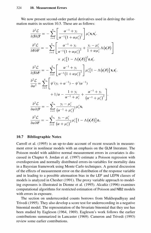
324 10. Measurement Errors

We now present second-order partial derivatives used in deriving the infor-mation matrix in section 10.5. These are as follows:

∂2L∂β∂β′ = −

n∑i=1

[α−1 + yi

α−1(1 + αµc

i

)2]

µci xi x′

i .

∂2L∂δ∂δ′ = −

n∑i=1

[α−1 + yi

α−1(1 + αµc

i

)2 + yi − µci

1 + αµci

(z′

iδ)]

× µci

[1 −

(z′

iδ)]2

zi z′i .

∂2L∂β∂δ′ = −

n∑i=1

[α−1 + yi

α−1(1 + αµc

i

)2]

µci

[1 −

(z′

iδ)]

xi z′i .

∂2L∂α2

=n∑

i=1

[ψ ′(yi + α−1) − ψ ′(α−1)

+ 1/α − 1 + yi

α−1 + µci

+ α−1 + yi(α−1 + µc

i

)2].

∂2L∂α∂β′ = −

n∑i=1

yi − µci(

α−1 + µci

)2 µci xi

∂2L∂α∂δ′ = −

n∑i=1

yi − µci(

α + µci

)2 µci

[1 −

(z′

iδ)]

zi .

10.7 Bibliographic Notes

Carroll et al. (1995) is an up-to-date account of recent research in measure-ment error in nonlinear models with an emphasis on the GLM literature. ThePoisson model with additive normal measurement errors in covariates is dis-cussed in Chapter 6. Jordan et al. (1997) estimate a Poisson regression withoverdispersion and normally distributed errors-in-variables for mortality datain a Bayesian framework using Monte Carlo techniques. A general discussionof the effects of measurement error on the distribution of the response variableand in leading to a possible attenuation bias in the LEF and LEFN classes ofmodels is analyzed in Chesher (1991). The proxy variable approach to model-ing exposures is illustrated in Dionne et al. (1995). Alcaniz (1996) examinescomputational algorithms for restricted estimation of Poisson and NB2 modelswith errors in exposure.

The section on underrecorded counts borrows from Mukhopadhyay andTrivedi (1995). They also develop a score test for underrecording in a negativebinomial model. The representation of the bivariate binomial that they use hasbeen studied by Eagleson (1964, 1969). Eagleson’s work follows the earliercontributions summarized in Lancaster (1969). Cameron and Trivedi (1993)review some earlier contributions.

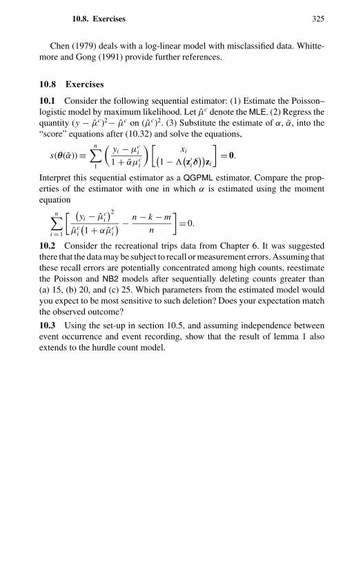
10.8. Exercises 325

Chen (1979) deals with a log-linear model with misclassified data. Whitte-more and Gong (1991) provide further references.

10.8 Exercises

10.1 Consider the following sequential estimator: (1) Estimate the Poisson–logistic model by maximum likelihood. Let µc denote the MLE. (2) Regress thequantity (y − µc)2− µc on (µc)2. (3) Substitute the estimate of α, α, into the“score” equations after (10.32) and solve the equations,

s(θ(α)) ≡n∑1

(yi − µc

i

1 + αµci

)[xi(

1 − (z′

iδ))

zi

]= 0.

Interpret this sequential estimator as a QGPML estimator. Compare the prop-erties of the estimator with one in which α is estimated using the momentequation

n∑i = 1

[ (yi − µc

i

)2µc

i

(1 + αµc

i

) − n − k − m

n

]= 0.

10.2 Consider the recreational trips data from Chapter 6. It was suggestedthere that the data may be subject to recall or measurement errors. Assuming thatthese recall errors are potentially concentrated among high counts, reestimatethe Poisson and NB2 models after sequentially deleting counts greater than(a) 15, (b) 20, and (c) 25. Which parameters from the estimated model wouldyou expect to be most sensitive to such deletion? Does your expectation matchthe observed outcome?

10.3 Using the set-up in section 10.5, and assuming independence betweenevent occurrence and event recording, show that the result of lemma 1 alsoextends to the hurdle count model.

CHAPTER 11

Nonrandom Samples and Simultaneity

11.1 Introduction

This chapter deals with the topic of valid inference about the population givensamples that are not simple random samples. There are several well-known waysin which departures from simple random sampling occur. They include choice-based sampling and endogenous stratified sampling, endogenous regressors,and sample selection.

The departure from simple random sampling may cause the sample proba-bility of observations to differ from the corresponding population probabilities.In general such a divergence leads to models in which simple conditioning onexogenous variables does not lead to consistent estimates of the populationparameters. These topics have been studied in depth in the discrete choice liter-ature (Manski and McFadden, 1981). The analysis of count data in the presenceof such complications is relatively underexplored.

A second topic considered in this chapter is endogenous regressors. Ignor-ing the feedback from the response variable to the endogenous regressor leadsin general to invalid inferences. The estimation procedure should allow forstochastic dependence between the response variable and endogenous regres-sors. In considering this issue the existing literature on simultaneous equationestimation in nonlinear models is of direct relevance (Amemiya, 1985). Thismaterial is a continuation of section 8.2.

The third topic considered is sample selection in count regression, whichalso is closely related to issues of simultaneity and nonrandom sampling.

Section 11.2 analyzes the consequences of choice-based sampling in generaland stratified random sampling with specific reference to standard count mod-els. Section 11.3 is a continuation of section 8.2, in which simultaneity issuesin count models and GMM estimation were discussed. The topic of GMM isstudied further in section 12.2. Finally, section 11.4 deals with sample selectionproblems, which is another type of departure from random sampling.

11.2 Alternative Sampling Frames

Simple random samples and exogenous sampling serve as benchmarks forother cases. They are described in sections 11.2.1 and 11.2.2. They generate a

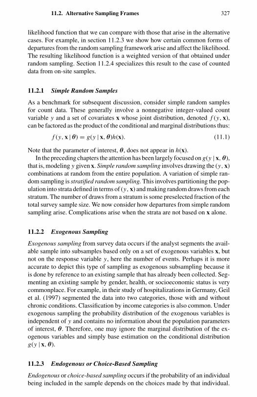
11.2. Alternative Sampling Frames 327

likelihood function that we can compare with those that arise in the alternativecases. For example, in section 11.2.3 we show how certain common forms ofdepartures from the random sampling framework arise and affect the likelihood.The resulting likelihood function is a weighted version of that obtained underrandom sampling. Section 11.2.4 specializes this result to the case of counteddata from on-site samples.

11.2.1 Simple Random Samples

As a benchmark for subsequent discussion, consider simple random samplesfor count data. These generally involve a nonnegative integer-valued countvariable y and a set of covariates x whose joint distribution, denoted f (y, x),can be factored as the product of the conditional and marginal distributions thus:

f (y, x |θ) = g(y | x,θ)h(x). (11.1)

Note that the parameter of interest, θ, does not appear in h(x).In the preceding chapters the attention has been largely focused on g(y | x,θ),

that is, modeling y given x. Simple random sampling involves drawing the (y, x)combinations at random from the entire population. A variation of simple ran-dom sampling is stratified random sampling. This involves partitioning the pop-ulation into strata defined in terms of (y, x) and making random draws from eachstratum. The number of draws from a stratum is some preselected fraction of thetotal survey sample size. We now consider how departures from simple randomsampling arise. Complications arise when the strata are not based on x alone.

11.2.2 Exogenous Sampling

Exogenous sampling from survey data occurs if the analyst segments the avail-able sample into subsamples based only on a set of exogenous variables x, butnot on the response variable y, here the number of events. Perhaps it is moreaccurate to depict this type of sampling as exogenous subsampling because itis done by reference to an existing sample that has already been collected. Seg-menting an existing sample by gender, health, or socioeconomic status is verycommonplace. For example, in their study of hospitalizations in Germany, Geilet al. (1997) segmented the data into two categories, those with and withoutchronic conditions. Classification by income categories is also common. Underexogenous sampling the probability distribution of the exogenous variables isindependent of y and contains no information about the population parametersof interest, θ. Therefore, one may ignore the marginal distribution of the ex-ogenous variables and simply base estimation on the conditional distributiong(y | x,θ).

11.2.3 Endogenous or Choice-Based Sampling

Endogenous or choice-based sampling occurs if the probability of an individualbeing included in the sample depends on the choices made by that individual.

328 11. Nonrandom Samples and Simultaneity

The practical significance of this is that consistent estimation of θ can no longerbe carried out using the conditional population density g(y | x) alone. The effectof the sampling scheme must also be taken into account.

In what follows, f denotes the joint, g the conditional, and h the marginaldensities. For further analysis we distinguish the sampling probability from thepopulation probability by superscript s on f (·) and h(·). We have

f s(y, x) = g(x | y)hs(y),

which can be reexpressed using the relations

f (y, x) = g(y | x)h(x),

= g(x | y)h(y),

where the marginal distributions are h(x) = ∑y f (y, x) and h(y) = ∫ g(y | x)×h(x) dx. Combining the above, we obtain

f s(y, x |θ) = f (y, x)hs(y)

h(y)

= g(y | x,θ)h(x)hs(y |θ)∫g(y | x,θ)h(x) dx

= g(y | x,θ)ω(y, x |θ),

where

ω(y, x |θ) = h(x)hs(y |θ)∫g(y | x,θ)h(x) dx

.

The log-likelihood function based on f s(y, x) is

L(θ | y, x) =n∑

i=1

ln g(yi | xi ,θ) +n∑

i=1

ln ω(yi , xi |θ). (11.2)

This can be interpreted as weighted log-likelihood, or log-likelihood based onweighted probabilities, where the weights ωi are ratios of sample and populationprobabilities and differ from unity (as in simple random samples). If thereexists prior information on the weights, then likelihood estimation based onweighted probabilities is straightforward. In the more usual situation in whichsuch information is not available, estimation is difficult because the distributionof x is involved. The literature on the estimation problem in the context ofdiscrete choice models is extensive (Manski and McFadden, 1981).

Standard conditional estimation considers the case when f s(y, x) = f (y, x).Thenω(y, x |θ) = h(x), which does not depend onθ, and maximizingL(θ | y, x)with respect to θ is the same as just considering the first term in (11.2). Iff s(y, x) = f (y, x), however, analysis using standard conditional estimation,which ignores the last term, leads to inconsistent estimates of θ.

11.2. Alternative Sampling Frames 329

11.2.4 Counts with Endogenous Stratification

Count data are sometimes collected by on-site sampling of users. For exam-ple, on-site recreational or shopping mall surveys (Shaw, 1988; Englin andShonkwiler, 1995; Okoruwa, Terza, and Nourse, 1988) may be carried outto study the frequency of use, often using travel-cost models. Such samplesinvolve truncation because only those who use the facility at least once are in-cluded in the survey. Furthermore, even among users the likelihood of beingincluded in the sample depends on the frequency of use. The latter feature ofthe sample is also called endogenous stratification or sampling because theselection of persons surveyed is based on a stratified sample, with random sam-pling within each stratum, the latter being defined by the number of events ofinterest.

Endogenous stratification has some similarities with choice-based sampling.As in that case, lower survey costs provide an important motivation for usingstratified samples in preference to simple random samples. It requires a verylarge random sample to generate enough observations (information) about arelatively rare event, such as visiting a particular recreational site. Hence, it isdeemed cheaper to collect an on-site sample. However, the problem is that ofmaking inferences about the population from the sample. To do so we needthe relation between the sample frequency function and the population densityfunction (Amemiya, 1985, pp. 319–338; Pudney, 1989, pp. 102–105).

A major objective in the analyses of on-site samples is to estimate the un-derlying (latent) population demand function for the number of trips. This isusually specified as a function of travel cost to the site j by user i , denotedCi j , and the characteristics of the site j , z j , and of the user i , xi . That is,y∗

i = φ(Ci j , xi , z j ), where y∗i denotes the desired number of trips. The demand

(yi ) is only observed if y∗ > 0, that is, y = y∗, if y∗ > 0. The sample spacefor the on-site sample is 1, 2, . . . whereas the sample space for the simplerandom sample would be 0, 1, 2, . . .. Thus the first consequence of on-sitesampling is truncation at zero. If f (y | x) denotes the population density of y(the number of trips), then the truncated density is f (y | x)/Pr[y > 0].

To derive a density function suitable for analyzing on-site samples, the jointeffect of truncation and stratification has to be considered. Shaw (1988) con-sidered the estimation problem for the choice-based sample. First, assume thatin absence of endogenous stratification the probability density of visits by in-dividual i , given characteristics x0, is g(yi | x0). Suppose there are m sampledindividuals with x = x0. Then the probability that individual i is observed tomake y0 visits is

Pr[yi = y0 | x0] = Pr[sampled value is y0 and sampled individual is i]

= Pr[sampled value is y0] Pr[sampled individual is i]

= g(y0 | x0)yi

y1 + y2 + · · · + yi−1 + yi + · · · + ym.

330 11. Nonrandom Samples and Simultaneity

Next consider the probability of observing y0 visits across all individuals, notjust the i th individual, Pr[y = y0 | x0], denoted Pm . This is the weighted sumof probability of y0 visits, where the weight of individual i (i = 1, . . . , m) isy0/(y1 + y2 + · · · + yi−1 + y0 + yi+1 + · · · + ym):

Pm = g(y0 | x0)

(y0

y0 + y2 + · · · + yi−1 + yi + · · · + ym+ · · ·

+ y0

y1 + y2 + · · · + yi−1 + yi + · · · + y0

)= g(y0 | x0)

1

m

(y0

(y0 + y2 + · · · + yi−1 + yi + · · · + ym)/m+ · · ·

+ y0

(y1 + y2 + · · · + yi−1 + yi + · · · + y0)/m

).

If we let m → ∞, the denominators inside the brackets above approach thepopulation mean value of y, given x = x0,

E[y0 | x0] =∞∑

y0=1

y0g(y0 | x0).

Then,

limm→∞ Pm = g(y0 | x0)

1

m

(y0∑∞

y0=1 y0g(y0 | x0)+ · · · + y0∑∞

y0=1 y0g(y0 | x0)

)

= y0g(y0 | x0)∑∞y0=1 y0g(y0 | x0)

.

This argument and derivation show that the relation between the conditionaldensity, gs(yi |µi ) for the endogenously stratified sample, and the populationconditional density, g(yi | xi ), is given by

gs(yi |µi ) = g(yi | xi )yi∑∞

y0=1 y0g(y0 | xi )(11.3)

= g(yi | xi )ω(yi , µi ), (11.4)

where

ω(yi , µi ) = yi

µi.

The key result is (11.4). This expression specializes to the following if thepopulation density is P[µi ] :

gs(yi | µi ) = e−µi µyi −1i

(yi − 1)!, (11.5)

11.3. Simultaneity 331

where

E [yi | xi ] = µi + 1 (11.6)

V [yi | xi ] = µi . (11.7)

Notice that the sample displays underdispersion even though the populationshows equidispersion. Maximization of the likelihood based on (11.5) can beinterpreted as maximizing a weighted likelihood. The case considered here isa special case of the more general discussion of choice-based sampling in thepreceding section.

An interesting implication of the analysis is that there is a computationallysimple way of maximizing this particular weighted likelihood. This is achievedby making the transformation wi = yi − 1, because the resulting sample spacefor wi is the same as that for the regular Poisson likelihood for wi . That is,applying the Poisson model to the original data with 1 subtracted from ally observations yields consistent estimates of the population mean parameterbecause

e−µi µwii

wi != e−µi µ

yi −1i

(yi − 1)!, yi = 1, 2, . . . . (11.8)

Hence, estimation can be implemented with the usually available software forPoisson maximum likelihood, whereas maximum likelihood estimation basedon (11.5) requires additional (although not difficult) programming.

Although the support for the zero-truncated Poisson (section 4.5) and thechoice-based Poisson is the same, the two distributions are different. Specifi-cally, in the truncated Poisson case,

E[yi | yi ≥ 0] = µi/(1 − e−µi ) > V[yi | yi ≥ 0],

which implies underdispersion. Choice-based sampling also displays underdis-persion, but this arises from a shift in the probability distribution.

The approach developed here can be extended for any parent populationdensity by specializing (11.4). Englin and Shonkwiler (1995) substitute theweighted negative binomial in place of the weighted Poisson and show thatthe subtraction device shown above for the Poisson also works for the nega-tive binomial. Santos Silva (1997) considers the implications of unobservedheterogeneity in the same model.

11.3 Simultaneity

In this section we consider the application of instrumental variable estimatorsfor dealing with the problem of endogenous regressors. Our treatment explainshow the choice of optimal instruments is affected by the way the error termenters the model, and the assumptions about heteroskedasticity. The simplestway to treat the problem is given at the end of section 11.3.2.

332 11. Nonrandom Samples and Simultaneity

11.3.1 Alternative Approaches

In Chapter 8 we outlined several empirically interesting cases in which a countvariable was jointly determined with another discrete or continuous variable.An example from health economics of a simultaneous model involving countsis the joint model of health-insurance choice, a discrete variable, and a mea-sure of healthcare services utilized, a count variable (Cameron et al., 1988).Another example is a labor supply model with the number of children as anexplanatory variable. However, if fertility is treated as endogenous, an equationfor the number of children should be a part of the model (Browning, 1992,pp. 1464–1465).

A further motivation for simultaneous equation estimation comes from thecorrelation between unobserved heterogeneity and included regressors. Thecommon assumption that unobserved heterogeneity is uncorrelated with theregressors is not plausible if it is a consequence of omitted regressors, whichare likely to be correlated with the included ones (see section 8.2).

Consider the two-element vector y = (y1, y2)′ with joint density f (y | x,θ),where x is treated as nonstochastic. It is convenient to treat y1 as a count; y2

may be either discrete or continuous. The standard factorization is

f (y | x,θ) = g(y1 | x, y2,θ1)h(y2 | x,θ2), θ ∈ Θ.

The standard result is that y2 and x may be treated symmetrically if h(y2 | x)does not depend on θ1. Estimating the parameters θ1 by conditioning y1 on y2

does not yield consistent estimates if the marginal density of y2 depends on θ1,in which case y2 is said to be endogenous.

To deal with this case, several approaches have evolved. One approach is tojointly model (y1, y2)′. This full information approach is reviewed in Chapter 8.A limited information approach is based on specification of one or two momentsof g(y1 | x, y2,θ1). These are extensions of the GMM or instrumental variablemethods for linear models. Despite nonlinearity of moment equations, suchmoment-based methods are attractive. This is because maximum likelihoodestimation of θ is usually computationally cumbersome, as the joint likelihoodmay not have a closed-form expression. It is often difficult to establish themarginal distribution h(y2 | x), so estimation methods often focus on approachesthat do not require this step.

11.3.2 Additive Errors

For nonlinear simultaneous equations an instrumental variable procedure wasproposed by Amemiya (1974). This approach readily extends to the specialcase of Poisson-type regression with endogenous regressors. The key step is tospecify the conditional mean function with an additive error term.

First we consider estimation of an exponential regression with an additiveerror that is correlated with the regressors x. Let X denote n × k matrix ofregressors. Let µ = exp(Xβ) and u = y − exp(Xβ), where exp(Xβ) is an

11.3. Simultaneity 333

(n×1) vector of n conditional means. With endogenous regressors, E[u | x] = 0,which implies

E[X′(y − exp(Xβ))] = 0. (11.9)

Suppose we have available a set of r linearly independent instruments W, whereW is n × r and may include a subset of X, r ≥ dim(β). Assume W, satisfyE[(y − exp(Xβ)) | W] = 0, which implies

E[W′(y − exp(X′β))] = 0. (11.10)

Let PW = W(W′W)−1W′. Then from Chapter 2, the NLIV estimator βNLIV min-imizes

(y − µ(β))′ PW(y − µ(β)). (11.11)

Under regularity conditions (Amemiya, 1985, p. 246), if V[y] = σ 2In ,

βNLIV ∼ N

[β, σ 2

[(∂µ′

∂β

)PW

(∂µ

∂β′

)]−1]

, (11.12)

where a consistent estimator of σ 2 is given by

σ 2 = 1

n

n∑i=1

(yi − exp

(x′

i βNLIV

))2.

The asymptotic properties of this type of estimator are also studied in Burguette,Gallant, and Souza (1982), Hansen (1982), and Newey (1990a) and are reviewedin Chapter 2 in a slightly different notation.

The preceding results are general. This method is valid for count data butignores the integer nature of the data and instead models the conditional mean.A refinement needed for count data, however, is to relax the assumption ofhomoskedastic error. One can either use the estimator in (11.11) with a moregeneral form of the variance matrix than (11.12) or use another more efficientestimator.

Suppose we assume

E[(y − µ) (y − µ)′ | W] = Ω = Diag[σ 2

i

].

For example, under equidispersion,

Ω = Diag[µi ].

Ignoring this information implies that βNLIV is consistent but not efficient. Amore efficient estimator is obtained if the previous objective function is replacedby

(y − µ(β))′ PWΩ (y − µ(β)) , (11.13)

334 11. Nonrandom Samples and Simultaneity

where

PWΩ = W(W′ΩW)−1W′.

In implementing this estimator a two-step procedure is used in which a con-sistent estimator Ω = Diag[µi ] is obtained first, and then PWΩ is substitutedfor PWΩ in the objective function. Denote the resulting two-step estimator asβNLIV2. The previously given distributional result still applies after substitutingthe above expression for PWΩ. That is,

βNLIV2 ∼ N[β, [X′ΩPWΩΩX]−1], (11.14)

because ∂µ/∂β′ = −ΩX.Optimal instrumental variables, denoted W∗, are those that yield the smallest

asymptotic variances. In the present case the optimal instrumental variablematrix, using the results in section 2.5.3, is

W∗ = E[Ω−1 ∂µ

∂β′

∣∣∣∣W],which for µ= exp(x′β) specializes to just X if W = X (no endogenous regres-sors). The problem of obtaining an expression for W∗ is compounded furtherif there is heteroskedasticity of the type commonly assumed in count models,which makes the expression Ω−1[∂µ/∂β′] a complicated function of X andW, some of which are endogenous. The key problem is that an analytical ex-pression for the expectation E[Ω−1∂µ/∂β′ | W] is usually not available if theresidual function u is nonlinear in the unknown parameters. In the general casein which W = X, consistent estimation of W∗ is impossible, and one usuallyhas to settle for consistent rather than efficient estimation. If one accepts as aworking hypothesis that Ω = Diag[µi ] or its scalar multiple, then the resultinginstruments are W∗ = E[X | W]. This simple result depends on the assumptionthat µ = exp(x′β). Windmeijer and Santos Silva (1997) suggest that in practiceone should use the instrument set XA, obtained by augmenting X by variablesnot collinear with X.

11.3.3 Multiplicative Errors

Mullahy (1997b) and Windmeijer and Santos Silva (1997) have discussed theadditive versus multiplicative error formulations, and their impact on the choiceof optimal instruments. Suppose the conditional mean function is specified as

E[y | x, η] = exp(x′β, η), (11.15)

where for simplicity the subscript i is suppressed. The regression model with amultiplicative error is

y = exp(x′β + η) = exp(x′β) exp(η) = exp(x′β)ν, (11.16)

11.3. Simultaneity 335

where η is a stochastic error correlated with x. Such an assumption may berationalized in terms of some relevant but unobserved variables that are omit-ted from the regression. Endogeneity of some of the regressors implies thatE[ν | x] = 1. Though the stochastic error η is not additively separable fromexp(x′β), as required for the application of the standard NLIV approach, a trans-formation can put it in that form. Specifically, the regression model may bewritten as

T (y, x,β) − 1 = ν − 1, (11.17)

where T (y, x,β) = exp(−x′β)y. Assume we have instruments w that satisfy

E[ν − 1 | w] = 0. (11.18)

An NLIV procedure for consistent estimation of β is to minimize the objectivefunction (ν − 1)′PW(ν − 1), or to solve the orthogonality conditions,

E[W′(T(y, X,β) − 1)] = 0, (11.19)

where we have used matrix notation in (11.19).An important point is that instrumental variables that are orthogonal to a

multiplicative error ν are not in general orthogonal to an additive error u. Thespecification of the error term affects the objective function, the choice ofinstruments, and the estimates of β. As before, if V[ν] = Ω = Diag[µi ], theobjective function and the orthogonality conditions must be suitably modified.Specifically note that the optimal instruments in the multiplicative case aregiven by

W∗ = E[Ω−1∂ν/∂β′ | W].

Because ∂ν/∂β′ = ∂µ/∂β′, they differ from those in the additive case. How-ever, this discussion is subject to a caveat. Optimal instruments may have otherundesirable properties, motivating one to use a suboptimal set. This issue isanalyzed in section 2.5.3.

Finally note that, if the specification of the variance function is ignored,most of the discussion of this section is not tailored to count data models assuch. It applies more generally to models with exponential mean. However,heteroskedasticity is a major feature of count data, so customization to countmodels with given variance functions is useful. For simplicity, the foregoingdiscussion uses a variance function without a nuisance parameter, but extensionis feasible. Consistent estimation of such a nuisance parameter can be basedon a sequential two-step procedure. At the first stage NLIV is applied withoutheteroskedasticity adjustment. At the second stage the nuisance parameter isestimated using methods analogous to those discussed in section 3.2. Finally,although we have emphasized the single-equation NLIV estimation, as pointedout in Chapter 9 the approach can in principle be generalized to dynamic paneldata models (Blundell, Griffiths, and Windmeijer, 1995).

336 11. Nonrandom Samples and Simultaneity

11.3.4 Example

A two-variable model with interdependent count and binary outcome variablesis one of the most relevant. Windmeijer and Santos Silva (1997), for example,consider the following model, in which y1 is a count and y∗

2 is a latent variable,

y1i = exp(αy2i + x′

1iβ)+ u1i

y∗2i = γ y1i + x′

2iδ + u2i ,(11.20)

where

Cov[u1i , u2i ] =[σ 2

1i σ12i

σ12i 1

], (11.21)

where var (u2i ) = 1 is a necessary normalization. The latent variable and theobserved variable y2 are related by

y2i =

1 if y∗2i > 0,

0 otherwise.

This model is logically coherent, in the sense of satisfying the restriction

Pr[y2i = 1] + Pr[y2i = 0] = 1,

only if either α = 0 or γ = 0. Assuming the latter, endogeneity implies σ12i = 0.Suppose, to take account of endogeneity, the y1 equation is estimated afterreplacing y2 by its conditional mean, F(x′

2δ), where F(·) denotes the estimatedcdf of y2. This mimics the logic of instrumental variable estimation in linearsimultaneous equations models. In that case the procedure leads to consistentestimates. In the present case,

y1i = exp[αF(x′

2i δ)+ x′

1iβ]

exp[α(y2i − F

(x′

2i δ))]+ u1i ;

where, ignoring the estimation of δ, the zero mean “error term,” y2 − F(x′2δ),

depends on x2 through its variance F(x′2δ)[1 − F(x′

2δ)]. Estimation of the y1

equation with the conditional mean function exp[αF(x′2δ) + x′

1β] does notyield consistent estimates of the parameters. However, as shown above for themultiplicative error case, the NLIV estimator, with the instrumental variablematrix W = [F(x′

2δ) x2], is consistent.

11.4 Sample Selection

Sample selection bias, usually induced by a departure from simple randomsampling, is an important issue in microeconometrics and may arise in countmodels. Although the issue is a very general one (Heckman, 1976; Manski,1995), in econometrics it has usually been discussed in the context of a ratherspecial normal linear model with censoring. The standard formulation of the

11.4. Sample Selection 337

selection problem in this linear case does not cover three distinguishing fea-tures of count regression models: nonnegativity, discreteness of the dependentvariable, and the frequently observed high incidence of zero observations. Solu-tions to these problems have been discussed by Terza (1998) and Weiss (1995).Several of these involve application of numerical methods to overcome analyt-ically intractable expressions in the likelihood. Our exposition focuses on themethod, avoiding details of computation that can be found in the cited works.We consider both full information and limited information estimators. We beginby reviewing a commonly used approach in the standard bivariate normal casewith the regression/probit structure.

11.4.1 Normal Linear Case

In this subsection we sketch the well-known formulation of selection effect inthe linear model. Suppose one wants to make inferences about the effectivenessof a treatment, such as a training program for workers. The following twoequations describe the decision to participate in the treatment and the outcomemeasure, for example, post-training wage, y1:

y1 = x′β + αy2 + u

y∗2 = z′γ + ε

y2 =

1 iff y∗2 > 0

0 iff y∗2 ≤ 0,

(11.22)

where y2 = 1 for those who participate and y2 = 0 for those who do not.The variable y∗

2 is a latent participation propensity indicator that dependson z. The variable y2 may also be thought of as a censoring indicator. Fori = 1, . . . , n, variables (xi , y2i ) are always observed, but y1i is only observedif y2i = 1. If the latent variable is positive the individual participates in thetreatment, and otherwise not.

One objective of an empirical investigation may be to make inferences aboutthe average effect of the treatment on the outcome of a randomly selectedmember of the population, conditional on a given x vector. However, the partialobservability of y1 makes for a potential identification problem for Pr[y1 | x].This is seen from the total probability equation (Manski, 1995)

Pr[y1 | x] = Pr[y1 | x, y2 = 1]Pr[y2 = 1 | x]

+ Pr[y1 | x, y2 = 0]Pr[y2 = 0 | x].

The sampling process cannot identify the term Pr[y1 | x, y2 = 0]. As Manskiemphasizes, whenever the censoring probability Pr[y2 = 0 | x] is positive, theavailable empirical evidence places no restrictions on Pr[y1 | x]. To learn any-thing about E[y1 | x], restrictions must be placed on Pr[y1 | x]. Frequently, theserestrictions are strongly parametric; that is, identification is secured by as-suming particular functional forms for moment functions and distributions of

338 11. Nonrandom Samples and Simultaneity

random variables, frequently linearity and normality. Given these assumptions,the fully efficient MLE is obtained from the likelihood based on the expressionfor Pr[y1 | x] given above. The alternative is to make weaker assumptions andreach weaker conclusions.

It is assumed that

E[u | X, y2] = 0; E[ε | Z] = 0; E[uε′ | X, Z, y2] = 0,

and the two disturbances have a joint bivariate normal distribution with co-variance matrix Σ= [σ jk], j, k = 1, 2. If E[uε′ | X, Z, y2] = 0, the treatmentequation (for y2) may be estimated by probit MLE, and the outcome equation(for y1) by linear regression.

Now

E[y1i | xi , y2i = 1] = x′iβ + α + E[ui |xi , y2i = 1]

= x′iβ + α + E

[ui | εi > −z′

iγ]

= x′iβ + α + σ12√

σ22rMi + ui , (11.23)

where α is the treatment effect and E[ui |xi , y2i = 1] is the selection effect,rMi = φi/(1 −i ) denotes the inverse Mills ratio of standard normal pdf to thecdf, and ui is a zero mean disturbance.

The estimation of α will be contaminated unless we can control for theselection effect. For example, estimation of (β, α) by least squares assumingexogenous y2 variable yields an inconsistent estimate because of the selectioneffect. This occurs because y2 is not exogenous in the outcome equation; that is,E[uε] = 0. Alternatively, we may think of the inconsistency problem as causedby the omitted “regressor” rM . Consistent maximum likelihood and sequentialestimation procedures have been proposed (Maddala, 1983; Pudney, 1989). Anespecially popular estimator is the Heckman two-step sequential procedure inwhich a probit model is fitted first to y2i , and the estimated parameters are usedto estimate rM,i , denoted rM,i . The latter is substituted for the true unobservedvariable, and the linear regression equation is estimated. The estimator is con-sistent (Amemiya, 1985); the computation of its variance is complicated anduses the method given in section 2.5.4.

11.4.2 Selection Effect in a Count Model

The key feature of data that results in a selectivity bias is that some phenomenonof interest is not fully observed and certain observations are systematicallyexcluded from analysis. In a count model this can arise if the event counts areonly observed for a selected subpopulation. An example given by Greene (1994)considers the number of major derogatory reports for a sample of credit-cardholders. Suppose this sample were used to make inferences about the probability

11.4. Sample Selection 339

of loan default of a credit card applicant with specified characteristics. Such aninference would exhibit selectivity bias because it would be based only on majorderogatory reports of individuals who have already been issued credit cards.The sample would not be random if some individuals who might otherwisedefault on payments had their applications for credit cards turned down. Suchindividuals are underrepresented in the sample of existing card holders. Totackle the task of estimating the count model in the presence of selectivity bias,it is necessary to model both the process of issuing credit cards and the countsof major derogatory reports.

Several authors including Terza (1998) and Greene (1994, 1997b) havedeveloped full maximum likelihood and two-step procedures for a sample-selection model for count data. The model considered has one outcome (count)equation and one selection equation. Although the model can be generalized,in this section we review their approach in the simpler context in which one hastwo dependent variables, one of which is a binary outcome variable (y2) and theother a count variable (y1) that is observed for only one particular realization ofthe binary variable. The key analytical device for modeling selection effects insuch a model is to begin with a parametric count distribution for y1 conditionalon covariates x and heterogeneity ν, with the assumption that heterogeneity andthe disturbance term in the binary outcome model follow a bivariate normal dis-tribution. We observe whether or not y2 = 1 (e.g., whether or not a credit cardis issued), and y1 if y2 = 1 (e.g., number of major derogatory reports givenissued credit card).

The observed value of the binary variable y2, given exogenous variables z,is determined by

y2 =

1 if z′θ2 + ε > 00 otherwise.

The count variable y1 is observed only if y2 = 1. The joint distribution ofy1 and y2 is denoted Pr[y1, y2 = 1 | x, z,ν]. The distribution is conditionedon covariates x and unobserved heterogeneity term ν. The random variables ν

and ε are assumed to have a bivariate normal distribution with mean zero andCor[ν, ε] = ρ; V[ν] = σ 2; V[ε] = 1. Then the conditional distribution of εi

given νi is N[(ρ/σ ) νi , (1 − ρ2)].Maximum likelihood estimation is based on the joint density of y1i and

y2i = 1, and on the probability that y2i = 0. Then

L(β, θ2, ρ, σ ) =n∑

i=1

ln Pr[y1i , y2i = 1 | xi , zi , νi ]

+ ln Pr[y2i = 0 | zi ]. (11.24)

First we need to derive the detailed expressions for the two terms in thelog-likelihood. The first term is obtained by integrating out unobserved hetero-

340 11. Nonrandom Samples and Simultaneity

geneity from the conditional distribution of counts

Pr[y1i , y2i = 1 | xi , zi ] =∫ ∞

−∞Pr [y1i , y2i = 1 | wi , νi ] g(νi ) dνi

= Eν [Pr [y1i , y2i = 1 | wi , νi ]]

≈ 1

S

S∑s=1

Pr[y1i , y2i = 1 | wi , ν

si

], (11.25)

where wi = [xi , zi ], and the last line is an approximation to Eν [·] based onsimulated probability using pseudorandom draws νs

i from the distribution of ν,denoted g(ν). The details of how to draw and use the random numbers efficientlycan be found in Gourieroux and Monfort (1997).

Conditional on νi , y1i and y2i are independent, hence

Pr [y1i , y2i = 1 | wi , νi ] = Pr [y1i | xi , νi ] Pr [y2i = 1 | zi , νi ] ,

where the first term on the right-hand side is the conditional count distribution.The second term is

Pr[y2i = 1 | zi , νi ]

= Pr[εi > −z′

iθ2 | zi , νi]

=∫ ∞

−z′iθ2

(2π )−1/2(1 − ρ2)−1/2 exp

[− 1

2(1 − ρ2)

(εi − ρ

σνi

)dεi

]=

[(1 − ρ2)−1/2

(z′

iθ2 + ρ

σνi

)]. (11.26)

Let Pr [y1, y2 = 1 | w, ν, ε] denote the joint distribution of y1 and y2, condi-tional on w, (= [x, z]), ν, and ε. Integrating out ν we obtain

Pr[y1i , y2i = 1 | wi ]

=∫ ∞

−∞Pr[y1i | xi , νi ]

[(1 − ρ2)−1/2

(z′

iθ2 + ρ

σνi

)]× 1

σ√

2πexp

(− ν2

i

2σ 2

)dνi ,

= 1√π

∫ ∞

−∞exp(−u2

i

)Pr [y1i | xi , ui ]

[z′

iθ∗2 + τui

]dui ,

(11.27)

where the second line is obtained by a change of variable u = ν/√

2σ 2, δ =σ/

√2σ 2, τ = √

2ρ/(1−ρ2)1/2, θ∗2 = θ2/(1−ρ2)1/2. This expression involves

Pr [y1i | xi , ui ] which is the heterogeneity-conditional distribution of the counts,specified as Poisson by both Terza and Greene.

11.4. Sample Selection 341

Integrating out νi from Pr [y2i = 0 | zi , νi ] in (11.26) yields the expressionfor the second term in the log-likelihood,

Pr [y2i = 0 | zi ] =∫ ∞

−∞

(1 − Pr

[εi > −z′

iθ2 | zi , νi])

g(νi ) dνi

= 1√2π

∫ ∞

−∞exp(−u2

i

)[−(z′

iθ∗2 + τui

)]dui

= EνPr[εi < −z′

iθ2 | zi , νi]

≈ 1

S

S∑s=1

Pr[εi < −z′

iθ2 | zi , νsi

]. (11.28)

The log-likelihood is constructed using the two terms (11.28) and (11.27),

L(β, θ2, ρ, σ ) =n∑

i=1

ln Pr [y1i , y2i = 1 | wi ]

+n∑

i=1

ln Pr [y2i = 0 | zi ] . (11.29)

The maximization of this likelihood function requires either numerical inte-gration or simulation as illustrated in section 4.9. The SML maximizes

L(β, θ2, ρ, σ ) =n∑

i=1

ln

(1

S

S∑s=1

Pr[y1i , y2i = 1 | wi , ν

si

])

+n∑

i=1

ln

(1

S

S∑s=1

Pr[εi < −z′

iθ2 | zi , νsi

]).

(11.30)

The expected values of random functions, expressed as integrals in the log-likelihood, are approximated by a sample mean of S simulated values of theseterms based on random draws us

i , s = 1, . . . , S. In other words, the probabilitiesin the log-likelihood, expressed as integrals, are approximated by sample meansof their simulated values. The resulting expression is then maximized in theusual way.

Although the method is computationally intensive, Greene’s (1997b) illus-trative application shows that computation is manageable.

Weiss (1995) proposes an alternative method for modeling sample selectionwith count data, based on Lee (1983). The marginal distributions of the randomvariables ν and ε are specified. With known marginals, transformations to con-vert these random variables to jointly normal variables can be found. Let G(ν)denote the distribution function cdf of ν, and let there be a function h(νi ) suchthat

εi = ρh(νi ) + ξi , (11.31)

342 11. Nonrandom Samples and Simultaneity

where ξi | νi ∼ N[0, σ 2ξ ]. Here ρ is the correlation parameter. For example, as-

sume gamma heterogeneity and consider a transformation of νi such that theresulting variable is linearly related to (correlated with) εi . That is, the trans-formation h can be found using

[h(νi )] = G(νi )

h(νi ) = −1[G(νi )] ,(11.32)

then (11.31) may be substituted into the expression for f (y1, y2 | w). Maximiz-ing the likelihood based on this approach still requires numerical integration(Weiss, 1995).

11.4.3 Sequential Estimation

In view of the computational burden of the full information approach, an analogof the Heckman two-step approach (see section 11.4.1) has some appeal. Usingessentially the same set-up given previously, the conditional mean of y1 is givenby

E[y1i | y2i = 1] = exp

[x′

iβ + σ 2

2

]((z′

iθ2 + ρσ)

(z′

iθ2) )

= exp[x′

iβ∗] (

(z′

iθ2 + ρσ)

(z′

iθ2) )

, (11.33)

where β∗ is the same as β apart from the intercept term, which is shifted byσ 2/2, (Johnson, Kotz, and Balakrishnan, 1994, p. 241). This regression may beestimated by NLS after substituting in the first stage estimates of θ2 denoted θ2.This step introduces heteroskedastic errors into the regression and complicatesthe estimation of the asymptotic covariance matrix as seen in section 2.5.4. If ρ

or σ = 0, the term in the square brackets on the right becomes 1, indicating zerosample selection bias. Thus, the effect of sample selection on the exponentialconditional mean of the count equation is multiplicative, not additive as in thenormal linear case. This suggests that an ad hoc adjustment based on adding theMill’s ratio to the conditional mean by analogy with the linear case is flawed.

11.4.4 Two-Part Models

The preceding analysis can be used to shed additional light on the two-part(hurdle) model discussed in section 4.7.1. Suppose we reinterpret the abovemodel as follows. Let the binary outcome model refer to the outcomes y1 = 0and y1 > 0. If y2 = 1, we observe y1 > 0, otherwise we observe y1 = 0. Givenindependence of y1 and y2 for positive counts we get

Pr [y1, y2 = 1] = Pr [y1] × Pr [y2 = 1] .

11.5. Bibliographic Notes 343

For Pr [y1] we need a distribution for counts that take values 1, 2, . . . , and inpractice we use a truncated Poisson or NB for Pr [y1]. (This is similar to the Randtwo-part model used in modeling expenditures on healthcare in which Pr [y1]is lognormal to allow for only positive observations.) Then the log-likelihoodfor this model is given by

n∑i=1

[ln Pr[y1i | y1i > 0, xi ] + ln Pr[y2i = 1 | zi ]] . (11.34)

The log-likelihood is usually maximized by separately maximizing the twoterms in the sum, with the first part based on a standard count distribution andthe second part on probit or logit model. Although the covariates in the two partsare often the same, this is not necessary. A more general set-up also allows forpossible correlation between the two parts, as in the selectivity model, therebyjustifying an analysis parallel to that of the selection model. For example, thecount distribution could be Poisson conditioned on unobserved heterogeneity ν.The binomial distribution of y2 could be conditioned on another unobservedheterogeneity term ε, with the (ν, ε) bivariate normal. Likelihood analysis ofsuch a model requires numerical or Monte Carlo integration.

11.5 Bibliographic Notes

Manski and McFadden (1981) survey and discuss choice-based sampling in thecontext of discrete choice models. Recently the problem has received consider-able attention. For example, Imbens and Lancaster (1994) deal with issues thatare closely related to those arising in choice-based samples and give many use-ful references. The optimal instruments problem for heteroskedastic nonlinearmodels is discussed in Newey (1993).

CHAPTER 12

Flexible Methods for Counts

12.1 Introduction

In this chapter we examine methods for modeling count data that are moreflexible than those presented in previous chapters. The focus is on the cross-section case, although some of the methods given here have potential extensionto time series, multivariate or longitudinal count data, and treatment of sampleselection.

One type of flexible modeling is to specify low-order conditional momentsof the dependent variable, rather than the entire distribution. This moment-based approach has already been considered extensively in previous chapters.Here we extend it by considering higher-order moments. The emphasis is on themore difficult question of the most efficient use of the moments, with estimatorsderived using results on optimal GMM.

The core of the chapter considers two basic types of flexible model. First, weconsider a sequence of progressively more flexible parametric models, where theunderlying parameters in the sequence are tightly specified, for example, equalto a specified function of a linear combination of regressors and parameters.

Second, we consider models in which part of the distribution or generalfunctional form for the moment is tightly specified, but the remainder is flexiblymodeled. For example, the conditional mean may be the exponential of the sumof a linear combination of all but one regressor and a flexible function of theremaining regressor. A second example, in which the conditional mean functionis specified but the conditional variance is flexible, has already been consideredin earlier chapters but is covered in further depth here.

Some authors call the general approach considered in this chapter semi-parametric methods but we prefer the term flexible methods. Fully parametricregression methods specify the distribution of y given x, and the estimationproblem is finite-dimensional. An example is the NB2 model. Pure nonpara-metric methods specify no part of the distribution of y given x, leading to aninfinite-dimensional estimation problem. Even here some basic assumptionsare made. Thus, in kernel regression of y given x in the continuous data case, itis usually assumed that data are iid and homoskedastic. In principle any method

12.2. Efficient Moment-Based Estimation 345

between these extremes is semiparametric. For example, throughout this bookwe have often considered inference based on specification of only the con-ditional mean, or on specification of the conditional mean and variance, andthese moment methods might be called semiparametric. A tighter definition ofsemiparametric is that despite specification of part of the model, there is stillan infinite-dimensional parameter estimation problem. Using this definition,estimation based on specification of the conditional mean and variance is notsemiparametric.

Section 12.2 deals with efficient moment-based estimation. This has beenpresented in previous studies as an extension of quasilikelihood using the es-timating equation approach, presented in Chapter 2. Here we also cast this inthe GMM framework. In section 12.3 we consider flexible functional forms forparametric distributions for count data. These include models based on poly-nomial series expansion, and the family of modified power series distributions.In section 12.4 we consider more flexible models for the conditional mean,focusing on the case in which a functional form is given for part but not allof the conditional mean function. In section 12.5 we consider estimation if afunctional form is specified for the conditional mean but not for the conditionalvariance. Estimators of regression coefficients more efficient than those given inearlier chapters are presented. Section 12.6 presents an application that focuseson some methods presented in sections 12.3 and 12.4.

12.2 Efficient Moment-Based Estimation

Key features of count models may be expressed as conditional mean and vari-ance restrictions, avoiding possible misspecification that may occur in a fullparametric specification of the likelihood function. Estimation given correctspecification of the conditional mean is done using the GLM and Poisson PMLapproaches covered extensively in Chapters 2 and 3. Efficiency gains are pos-sible by additionally specifying higher-order conditional moments. In section12.2.1 we state key results obtained in studies that use estimating equation andQL approaches. These results are then derived in Section 12.2.2, using the GMMapproach. This is a good illustration of the usefulness of the GMM framework.

12.2.1 Estimating Equations and Quasilikelihood

The extended QL approach is a refinement of the moment-based approach dis-cussed in earlier chapters. The version given here owes much to Crowder (1987)and Godambe and Thompson (1989). In this approach the central focus of esti-mation is on an estimating equation, whose solution defines an estimator, ratherthan on an objective function that is maximized or minimized. See section 2.5.1for the general estimating equation approach. The equations are analogous tothe score equations in maximum likelihood theory, leading to the terminologyextended QL.

346 12. Flexible Methods for Counts

We consider models in which functional forms µi = µ(xi ,θ) and σ 2i =

ω(xi ,θ) are specified for the conditional mean and variance of the scalar de-pendent variable yi . Crowder (1987) proposed the following general estimatingequation

n∑i = 1

a(xi ,θ)(yi − µi ) + b(xi ,θ)

(yi − µi )

2 − σ 2i

= 0, (12.1)

where a(xi ,θ) and b(xi ,θ) are q × 1 nonstochastic functions of θ, the q × 1unknown parameter vector to be estimated. Typically, θ = (β′, α)′ where β arethe parameters in the mean function, and the parameter α appears, in additionto β, in the variance function. This class includes unweighted least squareswhere a(xi ,θ) = ∂µi/∂θ and b(xi ,θ) = 0; and QL estimation, in which casea(xi ,θ) = (1/σ 2

i ) ∂µi/∂θ and b(xi ,θ) = 0.Setting b(xi ,θ) = 0 in (12.1) yields estimating equations that are quadratic

in (yi − µi ). These quadratic estimating equations (QEEs) are a potential re-finement to the QL approach. QL estimation is an appropriate approach if thevariance specification is doubtful, whereas the quadratic approach is better ifthe variance specification is more certain. Cubic and higher-order terms maybe added if there is more information about higher moments, but the practicalusefulness of such extensions is uncertain.

If µi = µ(xi ,β) and σ 2i = ω(xi ,β, α) are correctly specified, and θQEE is

the solution to the QEE, then from the results of Crowder (1987) it is known thatthe estimator is consistent and asymptotically normal with variance V[θQEE] =A−1

n BnA−1′n , where

An = −n∑

i=1

ai

∂µi

∂θ′ + 2σi bi∂σi

∂θ′

, (12.2)

Bn =n∑

i=1

σ 2i

ai a′

i + σiγ1i(ai b′

i + bi a′i

)+ σ 2i (γ2i + 2)

(bi b′

i

),

(12.3)

where ai = a(xi ,θ) and bi = b(xi ,θ) are (k + 1) × 1 vectors and γ1i andγ2i denote the skewness and kurtosis coefficients. The sandwich form of thevariance matrix is used. Consistent estimation ofθ requires correct specificationof the first two moments of y, while V[θQEE] depends on the first four moments.If bi = 0, the asymptotic covariance matrix does not depend on skewness orkurtosis parameters. This is consistent with earlier results for QL estimation.

As already noted, minimization of the first term only in the objective functioncorresponds to QL estimation. The second term is identically zero in some cases,such as the LEF density for which the variance function fully characterizes thedistribution. In such a case specification of higher-order moments is redundant.In other cases, however, efficiency gains result from the inclusion of a correctlyspecified second term. An example of this follows.

12.2. Efficient Moment-Based Estimation 347

Dean and Lawless (1989b) and Dean (1991), following Firth (1987), Crowder(1987), and Godambe and Thompson (1989), have discussed the estimation of amixed Poisson model using extended QL approach. This employs the followingspecification of the first four moments of the NB2 model

E[yi | xi ] = µi = µi (xi ,β)

E[(yi − µi )2 | xi ] = σ 2i = µi (1 + αµi )

E[(yi − µi )3 | xi ] = σ 3i γ1i = σ 2

i (1 + 2αµi )

E[(yi − µi )4 | xi ] = σ 4i γ2i = σ 2

i + 6ασ 4i + 3σ 4

i ,

(12.4)

where α ≥ 0, and γ1i and γ2i denote skewness and kurtosis coefficients.Suppose one assumes that the first four moments are known, but does not

wish to use the negative binomial distribution. The optimal quadratic estimatingequations for estimation can be shown to be

n∑i=1

(yi − µi )

σ 2i

∂µi

∂β= 0, (12.5)

n∑i=1

(yi − µi )2 − σ 2

i

(1 + αµi )2− (yi − µi )(1 + 2αµi )

(1 + αµi )2

= 0. (12.6)

Given correct specification of the first four moments, these equations yield themost efficient estimator for (β, α). Given α, the solution of the first equationyields the QL estimate of β. This is the special case of (12.1) with

a(xi ,θ) =[ (

1/σ 2i

)(∂µi/∂β)

−(1 + 2αµi )/(1 + αµi )2

],

b(xi ,θ) =[

0

1/(1 + αµi )2

].

The limit distribution can be obtained using (12.2) and (12.3).Other estimators for α, given β, have been suggested in the literature; for

example, moment estimators that assume γ1i = γ2i = 0 and hence are lessefficient than the previous one if the higher moment assumptions given earlierare correct. Dean and Lawless (1989b) have evaluated the resulting loss of effi-ciency in a simulation context. Dean (1991) shows that the asymptotic varianceof β is unaffected by the choice of the estimating equation for α. An appli-cation to the mixed PIG regression is in Dean, Lawless and Willmot (1989).The practicality of improving efficiency of estimators based on higher ordermoment assumptions remains to be established.

348 12. Flexible Methods for Counts

12.2.2 Generalized Method of Moments

The literature generally does not motivate well the QEE estimator (12.1) andoptimal cases such as (12.5) and (12.6). Results on optimal GMM provide asimple way to obtain the optimal formulation of the QEE.

From section 2.5.3, the optimal GMM estimator for general moment condi-tion

E[ρ(yi , xi ,θ) | xi ] = 0, (12.7)

where (yi , xi ) is iid, is the solution to the system of equations

n∑i=1

h∗i (yi , xi ,θ) = 0, (12.8)

where

h∗i (yi , xi ,θ) = E

[∂ρ(yi , xi ,θ)′

∂θ

∣∣∣∣ xi

]× E[ρ(yi , xi ,θ)ρ(yi , xi ,θ)′ | xi ]−1ρ(yi , xi ,θ).

(12.9)

We apply this result to estimation based on the first two moments, in whichcase

ρ(yi , xi ,θ) =[ρ1(yi , xi ,θ)

ρ2(yi , xi ,θ)

]=[

yi − µi

(yi − µi )2 − σ 2i

]. (12.10)

The first two moments are specified to be those of the NB2 model

µi = µi (xi ,β)

σ 2i = µi (1 + αµi ).

(12.11)

Then θ = (β′, α)′. Note that the conditional mean function is not restricted tobe exponential. Note also that identification of θ in this case requires that bothρ1(·) and ρ2(·) appear in h∗

i (·) in (12.9).For notational simplicity drop the subscript i and the conditioning on xi in

the expectation. The first two terms in the right-hand side of (12.9) are

E

∂ρ1

∂β

∂ρ2

∂β

∂ρ1

∂α

∂ρ2

∂α

= E

−∂µ

∂β−2(y − µ) − 1 − 2αµ∂µ

∂β

0 −µ2

=

−∂µ

∂β−(1 + 2αµ)

∂µ

∂β

0 −µ2

, (12.12)

12.2. Efficient Moment-Based Estimation 349

and E

[ρ2

1 ρ1ρ2

ρ1ρ2 ρ22

]−1

=

E

[(y − µ)2 (y − µ)(y − µ)2 − σ 2

(y − µ)(y − µ)2 − σ 2 (y − µ)2 − σ 22

]−1

=[

σ 2 σ 3γ1

σ 3γ1 σ 4γ2 − σ 4

]−1

= 1

σ 6(γ2 − 1 − γ 2

1

) [σ 4γ2 − σ 4 −σ 3γ1

−σ 3γ1 σ 2

], (12.13)

using E[(y − µ)3 | x] = σ 3γ1 and E[(y − µ)4 | x] = σ 4γ2, where γ1 and γ2

denote skewness and kurtosis coefficients. Substituting (12.10) through (12.13)into (12.9) yields

[h∗

1(yi , xi ,θ)h∗

2(yi , xi ,θ)

]=

(σ 4

i γ2i −σ 4i

)−(1+2αµi )σ 3

i γ1i

σ 6i

(γ2i −1−γ 2

1i

) ∂µi

∂β

σ 3i γ1i −(1+2αµi )σ 2

i

σ 6i

(γ2i −1−γ 2

1i

) ∂µi

∂β

σ 3i γ1i µ

2i

σ 6i

(γ2i −1−γ 2

1i

) −µ2i σ

2i

σ 6i

(γ2i −1−γ 2

1i

)

×[

y − µi

(y − µi )2 − σ 2i

]. (12.14)

The optimal GMM estimator solves (12.8) with h∗(yi , xi ,θ) defined in (12.9).Its distribution can be obtained using (2.70) through (2.72) in Section 2.5.1.From (12.14), identification requires γ2i − 1 − γ 2

1i = 0 for all i .Comparing (12.14) with (12.1), the optimal GMM estimator in this case is of

the QEE form (12.1), with a(xi ,θ) and b(xi ,θ), respectively, equal to the firstand second columns of the first matrix in the right-hand side of (12.14), whichis a (k + 1) × 2 matrix.

Now specialize to the case in which the skewness and kurtosis parameters γ1i

and γ2i are the functions given in (12.4). Then, in section 12.7 it is shown that(σ 4

i γ2i − σ 4i

)− (1 + 2αµi )σ3i γ1i = σ 4

i

(γ2i − 1 − γ 2

1i

)σ 3

i γ1i − (1 + 2αµi )σ2i = 0 (12.15)

σ 6i

(γ2i − 1 − γ 2

1i

) = 2(1 + α)σ 2i .

Using these results, (12.14) reduces to[h∗

1(yi , xi ,θ)

h∗2(yi , xi ,θ)

]= 1

σ 2i

∂µi

∂β0

(1+2αµi )µ2i

2(1+α)σ 4i

µ2i

2(1+α)σ 4i

[ y − µi

(y − µi )2 − σ 2i

].

(12.16)

350 12. Flexible Methods for Counts

For σ 2i defined in (12.11), µ2

i /σ4i = 1/(1 + αµi )2. Thus (12.16) yields the op-

timal QEE estimator defined in (12.5) and (12.6) on premultiplication of (12.6)by the constant 2(1 + α).

The optimal GMM estimator requires specification of E[ρ(yi , xi ,θ)ρ(yi ,

xi ,θ)′ | xi ], which in this example requires specification of the first four mo-ments. Newey (1993) proposed a semiparametric method of estimation, whichreplaces these elements by nonparametric estimates. For example, an estimateof the (1, 1) element, E[(yi − µi )2 | xi ], may be formed from a kernel or seriesregression of (yi − µi )2 on an intercept, µi and µ2

i , where µi is a consistentestimator. A similar treatment may be applied to the other two elements.

Unfortunately, even after determining that θ is identified under GMM, thissemiparametric method may run into practical difficulties. First, if the individ-ually estimated elements are combined, there is no guarantee that the resultingestimate of E[ρ(yi , xi ,θ)ρ(yi , xi ,θ)′ | xi ] will be positive definite as required.Second, even if the procedure produces a positive definite estimate, the esti-mate may be highly variable. Finally, in small samples the resulting estimatormay be biased, perhaps badly so, as indicated by several studies of the GMMmethod (Smith, 1997). The econometric literature includes several studies inwhich use of a constant rather the “optimal” matrix E[ρiρ

′i | xi ] produced better

estimates.

12.3 Flexible Distributions Using Series Expansions

12.3.1 Seminonparametric Maximum Likelihood

Gallant and Nychka (1987) proposed approximating the distribution of an iidm-dimensional random variable y using a squared power series expansionaround an initial choice of density or baseline density, say f (y |λ). Thus,

h p(y |λ, a) = (Pp(y | a))2 f (y |λ)∫(Pp(z | a))2 f (z) dz

, (12.17)

where Pp(y | a) is an m-variate pth order polynomial, a is the vector of co-efficients of the polynomial, and the term in the denominator is a normaliz-ing constant. Squaring Pp(y | a) has the advantage of assuring that the den-sity is positive. This is closely related to the series expansions in Chapter8, where Pp(y | a) was not squared and emphasis was placed on choosingPp(y | a) to be the orthogonal or orthonormal polynomials for the baselinedensity f (y |λ).

The estimator of λ and a maximizes the log-likelihood∑n

i=1 ln h p(yi |λ, a).Gallant and Nychka (1987) show that under fairly general conditions if theorder p of the polynomial increases with sample size n then the estimatoryields consistent estimates of the density. This result holds for a wide rangeof choices of baseline density. The estimator is called the seminonparametric

12.3. Flexible Distributions Using Series Expansions 351

maximum likelihood estimator. It is called seminonparametric to reflect that itis somewhere between parametric – in practice a specific baseline density needsto be chosen – and nonparametric.

This result provides a strong basis for using (12.17) to obtain a class of flex-ible distributions for any particular data. There are, however, several potentialproblems. First, the method may not be very parsimonious. Thus a poor initialchoice of baseline density may require a fairly high-order polynomial, a po-tential problem even with relatively large data sets of, say, 1000 observations.Second, it may be difficult to obtain analytical expressions for the normalizingconstant, especially in the multivariate case. Third, the normalizing constantusually leads to a highly nonlinear log-likelihood function with multiple lo-cal maxima. Finally, Gallant and Nychka (1987) establish only consistency. Aswith similar nonparametric approaches, it is difficult to establish the asymptoticdistribution. One solution is to bootstrap, although the asymptotic properties ofthis particular bootstrap do not appear to have been established. Another solu-tion is to select a high-enough-order polynomial to feel that the data is beingwell fit by the model, assume this is the density of the dgp, and apply standardmaximum likelihood results. This is similar to starting with the Poisson, reject-ing this in favor of NB2, and then using usual maximum likelihood standarderrors of the NB2 model for inference.

Gallant and Tauchen (1989) and various coauthors in many studies haveapplied models based on (12.17) to continuous finance data. There the baselinedensity is the multivariate normal with meanµ and variance Σ, with a particulartransformation used so that the normalizing constant is simply obtained as aweighted sum of the first 2p moments of the univariate standard normal. Theyadvocate selecting the order of the polynomial on the basis of the BIC of Schwarz(1978), defined in section 5.7.1, which gives a relatively large penalty for lackof parsimony.

In the first application of these methods to count data, Gurmu, Rilstone, andStern (1998) proposed using a series expansion to model the distribution ofthe heterogeneity term in the Poisson model with random heterogeneity. Thismethod has also been applied by Gurmu and Trivedi (1996) and extended tohurdle models by Gurmu (1997). Cameron and Johansson (1997) instead usea series expansion to directly generalize and modify the Poisson density forthe dependent variable. We present this study in sections 12.3.2 and 12.3.3 anddefer presentation of the other studies to section 12.5.2, on flexible models forthe heterogeneity term.

12.3.2 General Results

We begin with a quite general presentation for the univariate case, before spe-cializing to count data with a Poisson density as a baseline in the next subsection.Derivations are given in Cameron and Johansson (1997).

Consider a scalar random variable y with baseline density f (y |λ), whereλ is possibly a vector. The density based on a squared polynomial series

352 12. Flexible Methods for Counts

expansion is

h p(y |λ, a) = f (y |λ)P2

p (y | a)

ηp(λ, a), (12.18)

where Pp(y | a) is a pth-order polynomial

Pp(y | a) =p∑

k=0

ak yk, (12.19)

a = (a0, a1, . . . , ap)′ with the normalization a0 = 1, and ηp(λ, a) is a normal-izing constant term that ensures that the density h p(y |λ, a) sums to unity.Squaring the polynomial ensures that the density is nonnegative. This is justthe univariate version of (12.17). It can be shown that

ηp(λ, a) =p∑

k=0

p∑l=0

akalmk+l , (12.20)

where mr ≡ mr (λ) denotes the r th moment (not centered around the mean) ofthe baseline density f (y |λ).

The moments of the random variable y with density h p(y |λ, a) can bereadily obtained from those of the baseline density f (y |λ) as

E[yr ] =∑p

k=0

∑pl=0 akalmk+l+r

ηp(λ, a). (12.21)

The r th moment of y generally differs from the r th moment of the baselinedensity. In particular, the mean for the series expansion density h p(y |λ, a)usually differs from that for the baseline density f (y |λ).

We consider estimation based on a sample (yi , xi ), i = 1, . . . , n of inde-pendent observations. Then yi | xi has density h p(yi |λi , ai ), where regressorscan be introduced by lettingλi or ai be a specified function of xi and parametersto be estimated. As a simple example, suppose λi is a scalar determined by aknown function of regressors xi and an unknown parameter vector β

λi = λ(xi ,β), (12.22)

and the polynomial coefficients a are unknown parameters that do not vary withregressors. The log-likelihood function is then

L(β, a) =n∑

i=1

ln f (yi | λ(xi ,β)) + 2 ln Pp(yi | a)

− ln ηp(λ(xi ,β), a), (12.23)

12.3. Flexible Distributions Using Series Expansions 353

with first-order conditions that, given ηp(λ, a) in (12.20), can be reexpressedas

∂L∂β

=n∑

i=1

∂ ln f (yi | λi )

∂λi−∑p

k=0

∑pl=0 akal∂mk+l,i/∂λi∑p

k=0

∑pl=0 akalmk+l,i

∂λi

∂β= 0,

(12.24)

∂L∂a j

=n∑

i=1

2

y j∑p

k=0 ak yk−

∑pk=0 akmk+ j,i∑p

k=0

∑pl=0 akalmk+l,i

= 0,

j = 1, . . . , p. (12.25)

Cameron and Johansson (1997) do not establish semiparametric consistencyof this method. Instead, the density with chosen p is assumed to be correctlyspecified. Inference is based on the standard result that the MLE for β and a isasymptotically normally distributed with variance matrix equal to the inverseof the information matrix, under the assumption that the data are generated by(12.18) and (12.22).

In principle this method is very easy to apply, provided analytical momentsof the baseline density are easily obtained. The maximum likelihood first-orderconditions simply involve derivatives of these moments with respect to λ, andeven then some optimization routines do not require specification of first deriva-tives.

In practice there are two potential problems. First, the objective function isvery nonlinear in parameters and there are multiple optima. This is discussed inthe next subsection. Second, these series expansion densities may not be veryparsimonious or may not fit data very well. The usefulness can really only beestablished by applications.

12.3.3 Poisson Polynomial Model

The preceding framework can be applied to a wide range of baseline densi-ties. Cameron and Johansson illustrated this method if baseline density is thePoisson, so f (y | µ) = e−µµy/y!. They called this model the PPp model, forPoisson polynomial of order p. Then λ = µ, and the normalizing constantηp(µ, a) defined in (12.20) and the moments E[yr ] defined in (12.21) are eval-uated using the moments mr (µ) of the Poisson, which can be obtained from themoment generating function using mr (µ) = ∂r exp(−µ + µet )/∂tr | t=0.

As an example the PP2 model is

h2(y | µ, a) = e−µµy

y!

(1 + a1 y + a2 y2)2

η2(a, µ), (12.26)

where

η2(a, µ) = 1 + 2a1m1 + (a21 + 2a2

)m2 + 2a1a2m3 + a2

2m4.

(12.27)

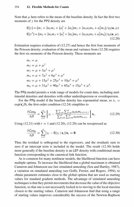
354 12. Flexible Methods for Counts

Note that µ here refers to the mean of the baseline density. In fact the first twomoments of y for the PP2 density are

E[y] = (m1 + 2a1m2 + (a21 + 2a2

)m3 + 2a1a2m4 + a2

2m5)/η2(a, µ)

E[y2] = (m2 + 2a1m3 + (a21 + 2a2

)m4 + 2a1a2m5 + a2

2m6)/η2(a, µ).

(12.28)

Estimation requires evaluation of (12.27) and hence the first four moments ofthe Poisson density; evaluation of the mean and variance from (12.28) requiresthe first six moments of the Poisson density. These moments are

m1 = µ

m2 = µ + µ2

m3 = µ + 3µ2 + µ3

m4 = µ + 7µ2 + 6µ3 + µ4

m5 = µ + 15µ2 + 25µ3 + 10µ4 + µ5

m6 = µ + 31µ2 + 90µ3 + 65µ4 + 15µ5 + µ6.

The PPp model permits a wide range of models for count data, including mul-timodal densities and densities with either underdispersion or overdispersion.

For the PPp model if the baseline density has exponential mean, so λi =exp(x′

iβ), the first-order condition (12.24) simplifies to

∂LPPp

∂β=

n∑i=1

yi −

∑pk=0

∑pl=0 akalmk+l+1,i∑p

k=0

∑pl=0 akalmk+l,i

xi . (12.29)

Using (12.21) with r = 1 and (12.20), (12.29) can be reexpressed as

∂LPPp

∂β=

n∑i=1

(yi − E[yi | xi ])xi = 0. (12.30)

Thus the residual is orthogonal to the regressors, and the residuals sum tozero if an intercept term is included in the model. The result (12.30) holdsmore generally if the baseline density is an LEF density with conditional meanfunction corresponding to the canonical link function.

As is common for many nonlinear models, the likelihood function can havemultiple optima. To increase the likelihood that a global maximum is obtainedCameron and Johansson use fast simulated annealing (Szu and Hartley, 1987),a variation on simulated annealing (see Goffe, Ferrier, and Rogers, 1994), toobtain parameter estimates close to the global optima that are used as startingvalues for standard gradient methods. The advantage of simulated annealingtechniques is that they permit movements that decrease the value of the objectivefunction, so that one is not necessarily locked in to moving to the local maximaclosest to the starting values. Cameron and Johansson find that using a rangeof starting values improves considerably the success of the Newton-Raphson

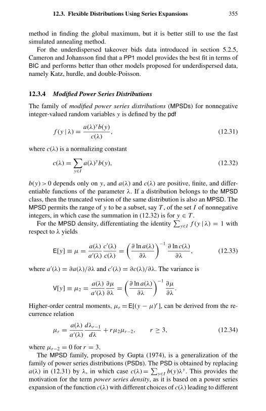
12.3. Flexible Distributions Using Series Expansions 355

method in finding the global maximum, but it is better still to use the fastsimulated annealing method.

For the underdispersed takeover bids data introduced in section 5.2.5,Cameron and Johansson find that a PP1 model provides the best fit in terms ofBIC and performs better than other models proposed for underdispersed data,namely Katz, hurdle, and double-Poisson.

12.3.4 Modified Power Series Distributions

The family of modified power series distributions (MPSDs) for nonnegativeinteger-valued random variables y is defined by the pdf

f (y | λ) = a(λ)yb(y)

c(λ), (12.31)

where c(λ) is a normalizing constant

c(λ) =∑y∈I

a(λ)yb(y), (12.32)

b(y) > 0 depends only on y, and a(λ) and c(λ) are positive, finite, and differ-entiable functions of the parameter λ. If a distribution belongs to the MPSDclass, then the truncated version of the same distribution is also an MPSD. TheMPSD permits the range of y to be a subset, say T , of the set I of nonnegativeintegers, in which case the summation in (12.32) is for y ∈ T .

For the MPSD density, differentiating the identity∑

y∈I f (y | λ) = 1 withrespect to λ yields

E[y] ≡ µ = a(λ)

a′(λ)

c′(λ)

c(λ)=(

∂ ln a(λ)

∂λ

)−1∂ ln c(λ)

∂λ, (12.33)

where a′(λ) = ∂a(λ)/∂λ and c′(λ) = ∂c(λ)/∂λ. The variance is

V[y] ≡ µ2 = a(λ)

a′(λ)

∂µ

∂λ=(

∂ ln a(λ)

∂λ

)−1∂µ

∂λ.

Higher-order central moments, µr = E[(y − µ)r ], can be derived from the re-currence relation

µr = a(λ)

a′(λ)

dλr−1

dλ+ rµ2µr−2, r ≥ 3, (12.34)

where µr−2 = 0 for r = 3.The MPSD family, proposed by Gupta (1974), is a generalization of the

family of power series distributions (PSDs). The PSD is obtained by replacinga(λ) in (12.31) by λ, in which case c(λ) = ∑y∈I b(y)λy . This provides themotivation for the term power series density, as it is based on a power seriesexpansion of the function c(λ) with different choices of c(λ) leading to different

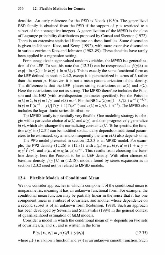
356 12. Flexible Methods for Counts

densities. An early reference for the PSD is Noack (1950). The generalizedPSD family is obtained from the PSD if the support of y is restricted to asubset of the nonnegative integers. A generalization of the MPSD is the classof Lagrange probability distributions proposed by Consul and Shenton (1972).There is an extensive statistical literature on these families. Some discussionis given in Johnson, Kotz, and Kemp (1992), with more extensive discussionin various entries in Kotz and Johnston (1982–89). These densities have rarelybeen applied in a regression setting.

For nonnegative integer-valued random variables, the MPSD is a generaliza-tion of the LEF. To see this note that (12.31) can be reexpressed as f (y|λ) =exp−ln c(λ) + ln b(y) + ln a(λ)y. This is exactly the same functional form asthe LEF defined in section 2.4.2, except it is parametrized in terms of λ ratherthan the mean µ. However, it is not a mean parameterization of the density.The difference is that the LEF places strong restrictions on a(λ) and c(λ).Here the restrictions are not as strong. The MPSD therefore includes the Pois-son and the NB2 (with overdispersion parameter specified). For the Poisson,a(λ) = λ, b(y) = 1/y! and c(λ) = eλ. For the NB2, a(λ) = [1−λ/(λ+α−1)]−1/α ,b(y) = (α−1 + y)/[(y + 1)(α−1) and c(λ) = λ/(λ + α−1). The MPSD alsoincludes the logarithmic series distributions.

The MPSD family is potentially very flexible. One modeling strategy is to be-gin with a particular choice of a(λ) and b(y), and then progressively generalizeb(y), which also changes the normalizing constant c(λ). To be specific, the func-tion b(y) in (12.31) can be modified so that it also depends on additional param-eters to be estimated, say a, and consequently the term c(λ) also depends on a.

The PPp model presented in section 12.3.3 is an MPSD model. For exam-ple, the PP2 density (12.26) is (12.31) with a(µ) = µ, b(y, a) = (1 + a1 y +a2 y2)2/y!, and c(µ, a) = η2(a, µ)/e−µ. This results from choosing the base-line density, here the Poisson, to be an LEF density. With other choices ofbaseline density f (y | λ) in (12.18), models found by series expansion as insection 12.3.2 need not be related to MPSD models.

12.4 Flexible Models of Conditional Mean

We now consider approaches in which a component of the conditional mean isnonparametric, meaning it has an unknown functional form. For example, theconditional mean function may be partially linear in the sense that it has onecomponent linear in a subset of covariates, and another whose dependence ona second subset is of an unknown form (Robinson, 1988). Such an approachhas been developed by Severini and Staniswalis (1994) in the general contextof quasilikelihood estimation of GLM models.

Consider a model in which the conditional mean of yi depends on two setsof covariates, xi and zi , and is written in the form

E[yi | xi , zi ] = µ(x′

iβ + γ (zi )), (12.35)

where µ(·) is a known function and γ (·) is an unknown smooth function. Such

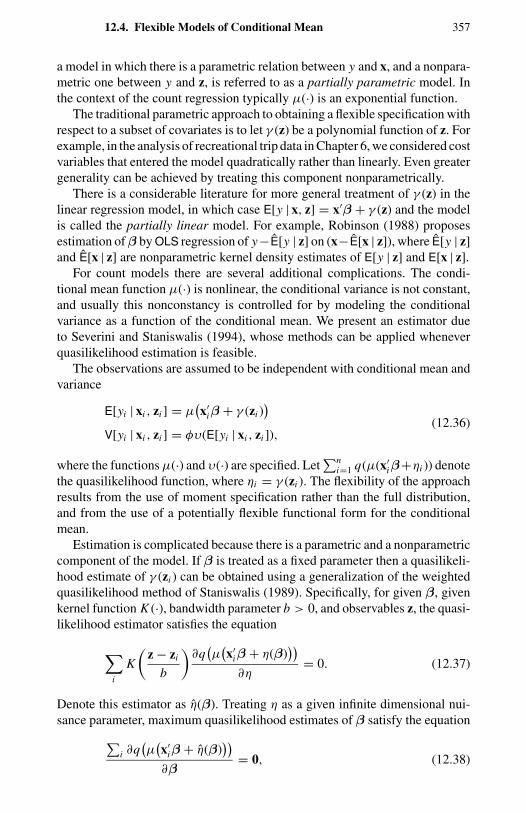
12.4. Flexible Models of Conditional Mean 357

a model in which there is a parametric relation between y and x, and a nonpara-metric one between y and z, is referred to as a partially parametric model. Inthe context of the count regression typically µ(·) is an exponential function.

The traditional parametric approach to obtaining a flexible specification withrespect to a subset of covariates is to let γ (z) be a polynomial function of z. Forexample, in the analysis of recreational trip data in Chapter 6, we considered costvariables that entered the model quadratically rather than linearly. Even greatergenerality can be achieved by treating this component nonparametrically.

There is a considerable literature for more general treatment of γ (z) in thelinear regression model, in which case E[y | x, z] = x′β + γ (z) and the modelis called the partially linear model. For example, Robinson (1988) proposesestimation ofβ by OLS regression of y−E[y | z] on (x−E[x | z]), where E[y | z]and E[x | z] are nonparametric kernel density estimates of E[y | z] and E[x | z].

For count models there are several additional complications. The condi-tional mean function µ(·) is nonlinear, the conditional variance is not constant,and usually this nonconstancy is controlled for by modeling the conditionalvariance as a function of the conditional mean. We present an estimator dueto Severini and Staniswalis (1994), whose methods can be applied wheneverquasilikelihood estimation is feasible.

The observations are assumed to be independent with conditional mean andvariance

E[yi | xi , zi ] = µ(x′

iβ + γ (zi ))

V[yi | xi , zi ] = φυ(E[yi | xi , zi ]),(12.36)

where the functions µ(·) and υ(·) are specified. Let∑n

i=1 q(µ(x′iβ+ηi )) denote

the quasilikelihood function, where ηi = γ (zi ). The flexibility of the approachresults from the use of moment specification rather than the full distribution,and from the use of a potentially flexible functional form for the conditionalmean.

Estimation is complicated because there is a parametric and a nonparametriccomponent of the model. If β is treated as a fixed parameter then a quasilikeli-hood estimate of γ (zi ) can be obtained using a generalization of the weightedquasilikelihood method of Staniswalis (1989). Specifically, for given β, givenkernel function K (·), bandwidth parameter b > 0, and observables z, the quasi-likelihood estimator satisfies the equation

∑i

K

(z − zi

b

)∂q(µ(x′

iβ + η(β)))

∂η= 0. (12.37)

Denote this estimator as η(β). Treating η as a given infinite dimensional nui-sance parameter, maximum quasilikelihood estimates of β satisfy the equation∑

i ∂q(µ(x′

iβ + η(β)))

∂β= 0, (12.38)

358 12. Flexible Methods for Counts

which is a parametric estimation problem. In general these equations are solvediteratively. The interested reader should refer to the original article for detailsof the asymptotic properties of this estimator.

In practice the user of this method needs to determine which variables con-stitute the z subset and which ones the x subset. Although such choices arecontext-specific, given the constraint that γ should be smooth, continuous vari-ables are the natural candidates for z. If the sample size is large and the di-mension of z not too large, then a computationally simpler alternative seems toapproximate γ (z) by a quadratic in z, as for instance in the recreational dataanalysis of Chapter 6, and then treat the estimation parametrically.

An alternative class of flexible models of the conditional mean, one embed-ded in the GLM framework, is the generalized additive model due to Hastieand Tibshirani (1990). Then the linear component x′β in the GLM class modelis replaced by an additive model of the form

∑kj=2 f j (x j ), where f j (·) are

nonparametric univariate functions, one for each covariate. Thus

E[yi | xi ] = µ

(β1 +

k∑j=2

f j (xi j )

),

where xi j is the j th component of xi , and µ(·) is specified. For Poisson regressionµ(·) = exp(·) and the conditional variance is a multiple of µ(·).

12.5 Flexible Models of Conditional Variance

Let us reconsider the mixture density

h(yi | xi ) =∫

f (yi | xi , νi )g(νi ) dνi , (12.39)

introduced in Chapter 4, where the density f (yi | xi , νi ) is the Poisson withconditional mean µiνi = exp(x′

iβ)νi . Unlike Chapter 4, the distribution of theunobserved heterogeneity component is treated as unknown. In this section weconsider flexible models for the mixture density g(νi ), leading to more flexiblemodels for h(yi | xi ). The first method considers mixtures of densities, whilethe second method uses a series expansion.

At the end of this section we present an adaptive estimation procedure thatprovides efficient estimates of the conditional mean parameters, controlling forheteroskedasticity by nonparametric estimation of the conditional variance.

12.5.1 Mixture Models for Unobserved Heterogeneity

As in section 4.8, consider a discrete representation of g(ν), so that the marginaldistribution may be written as

h(yi | xi ,β) =C∑

j=1

f (yi | xi ,β, ν j )π j (ν j ), (12.40)

12.5. Flexible Models of Conditional Variance 359

where ν j , j = 1, . . . , C , is an estimated support point for the distribution ofunobserved heterogeneity and π j is the associated probability with π j ≥ 0 and∑

j π j = 1.For the Poisson with exponential mean, this representation of heterogeneity

may be interpreted as a random-intercept model in which the intercept is (β0 +ν j ) with probability π j . This is detailed in section 4.8. The subpopulation witheach intercept is treated as a “type,” and the number of types, C , is estimatedfrom the data along with (π j ,β).

The method has both a nonparametric component, because it avoids distri-butional assumptions on ν, and a parametric component, the density f (y | x,β, ν). It is standard terminology in the statistic literature to call the estimatoran SPMLE if C is taken as given and maximum likelihood estimation is donefor the unknown parameters (β, π j ).

As an example, if f (yi | xi ,β, ν j ) in (12.40) is the Poisson density withparameter µiν j ,with µi = µ(xi ,β), the log-likelihood is

LSP(β,π) =n∑

i=1

[yi ln (µi ) − ln (yi !) + ln

(C∑

j=1

exp(−µiν j )νyi

j π j

)].

(12.41)

Estimation of this model is discussed in section 4.8.

12.5.2 Series Expansions for Unobserved Heterogeneity

This section outlines estimation of the Poisson model with exponential meanand a random heterogeneity component ν whose density g(ν) is modeled bya series expansion. The method was proposed by Gurmu, Rilstone, and Stern(1998), who call it SPMLE. The goal is a flexible model specification that avoidsstrong parametric assumptions about the distribution of ν.

If y conditional on µ and ν is P[µν] distributed, the mixture density (12.39),suppressing the subscript i , is

h(y | µ) =∫

e−µν(νµ)y

y!g(ν) dν

= µy

y!

∫ν ye−µνg(ν) dν. (12.42)

Gurmu et al. propose approximating the unknown mixture density g(ν) by asquared pth-order polynomial expansion of form (12.17), say g∗

p(ν), and an-alytically calculating the integral in (12.42) with respect to g∗

p(ν) rather thang(ν). The two-parameter gamma is used as the baseline density, because thisrestricts ν > 0, and more importantly because the leading term in the expansionis then the gamma, which from Chapter 4 leads to h(y | µ) being the standardNB2 density. An orthonormal polynomial series expansion is used (see Chap-ter 8) in which the orthogonal polynomials for the gamma are the orthonormalgeneralized Laguerre polynomials.

360 12. Flexible Methods for Counts

Specifically, the approximating density is

g∗p(ν | λ, γ ) = f (ν | λ, γ )

P2p (ν | λ, γ, a)

ηp(λ, γ, a), (12.43)

where f (ν | λ, γ ) is the two-parameter gamma density

f (ν | λ, γ ) = νγ−1λγ

(γ )e−λν, (12.44)

P2p (ν | α, γ, a) is the pth-order orthonormal generalized Laguerre polynomial

P2p (ν | λ, γ, a) =

p∑k=0

akη−1/2k Qk(ν) (12.45)

with the kth-order orthogonal generalized Laguerre polynomial defined by

Qk(ν) =k∑

l=0

(k

l

)(k + γ )

(l + γ )(k + 1)λl(−ν)l , (12.46)

orthonormalization is achieved by premultiplying Qk(ν) in (12.45) by η−1/2k

with

ηk = (k + γ )

(γ )(k + 1), (12.47)

and orthonormalization leads to the normalizing constant being simply

ηp(λ, γ, a) =p∑

k=0

a2k . (12.48)

Clearly, evaluating∫

ν ye−µνg(ν) dν in (12.42) is not straightforward forg(ν) = g∗

p(ν | λ, γ ) defined by (12.43) through (12.48). Gurmu et al. observethat if ν has density g(ν), the moment generating function of ν is

Mν(t) =∫

etνg(ν) dν,

with yth-order derivative

M(y)ν (t) = ∂ yMν(t)/∂t y =

∫ν yetνg(ν) dν.

Thus (12.42) can be re-expressed as

h(y | µ) = [µy/y!]M(y)ν (−µ). (12.49)

12.5. Flexible Models of Conditional Variance 361

Gurmu et al. obtain the analytical expression for M∗ν,p(t), the moment generat-

ing function for g∗p(ν|λ, γ ) defined by (12.43) through (12.48), and its yth-order

derivative M∗(y)ν,p (t) = ∂ yM∗

ν,p(t)/∂t y . Evaluation at t = −µ yields

M∗(y)ν,p (−µ) =

(1 + µ

λ

)−γ(γ )

(λ + µ)y

(p∑

k=0

a2k

)−1 p∑k=0

p∑l=0

akal (ηkηl)1/2

×k∑

r=0

l∑s=0

(k

r

)(l

s

)(γ + r + s + y)

(γ + r )(γ + s)

(−1 − µ

λ

)−(r+s).

(12.50)

Premultiplication by [µy/y!] yields at last the approximating density for thecount variable.

The log-likelihood function for a sample of size n is

lnL(β, γ, λ, a) =n∑

i=1

yi ln µi − ln(yi !) + ln

(M∗(yi )

ν,p (−µi ))

,

(12.51)

where in practice µi = exp(x′iβ). The MLE is obtained in the usual way. Identi-

fication requires that E[νi ] = M∗(1)ν,p (0) = 1 and a0 = 1. A formal statement and

proof of the semiparametric consistency of this procedure is given in Gurmuet al. (1998), but to date its asymptotic distribution as p → ∞ has not beenestablished.

This type of mixture representation generalizes the treatment of heterogene-ity but does not alter the specification of the conditional mean in any way. Oneadvantage of using Laguerre polynomial expansion is that the leading term is thegamma density, which has been used widely as a mixing distribution in countand duration literature. Thus, if higher terms in the expansion vanish and γ = λ,we obtain the popular NB2 model of the earlier chapters, with γ = λ = α−1.Further, if γ −1 = λ−1 → 0 and a j = 0 for j ≥ 1, the Poisson model is obtained.Unlike semiparametric methods based on discrete mixtures, such as that in thepreceding subsection, the series expansion method provides smooth estimationof the distribution of unobserved heterogeneity.

This form of heterogeneity representation is computationally demanding.The complexity of the last term in the log-likelihood hinders an analyticalstudy of the likelihood. As with other series-based likelihoods there remains apossibility of multiple maxima and at present no test is available for a globalmaximum. Gurmu et al. compute the standard errors by computer-intensivebootstrap methods. Alternatively, if the estimated value of p is treated as correct,one can use the outer product of numerically evaluated gradients of (12.51). Asin other studies, information criteria are used to select the number of terms pin the expansion.

Gurmu et al. show that this method can be extended to Poisson models withcensoring, truncation, and excess zeros and ones. They apply the model to

362 12. Flexible Methods for Counts

censored data on the number of shopping trips to a shopping mall in a monthtaken by 828 shoppers, where 7.9% of the observations are right-censored dueto the highest category being recorded as 3 or more and the data are somewhatoverdispersed with sample variance 2.1 times the sample mean. They prefera model with p = 2, meaning two terms more than the NB2. Application byGurmu and Trivedi (1996) to uncensored data is presented in section 12.6. InGurmu (1997) the method is extended and applied to the hurdle model, leadingto a model that nests the hurdle specifications considered in section 4.7. Al-though appealing in principle, a potential problem with the hurdle specificationis overfitting due to estimation of two parts of the model.

12.5.3 Nonparametric Estimation of Variance

An alternative to flexible specification of the variance function is to impose noalgebraic form on the variance function but to treat it nonparametrically. In idealcircumstances one can obtain estimates of the conditional mean parametersthat are as efficient if the variance function is unspecified as they are if it isspecified. Then the estimation method is called adaptive. Note that this is moreambitious than methods presented in Chapter 3 for unknown variance function.There, if the variance function was not specified or at least not assumed to becorrectly specified, the goal was to obtain consistent parameter estimates andvalid standard errors. Efficient estimation was not a goal.

Here we present the adaptive method of Delgado and Kniesner (1997) forheteroskedasticity of unknown functional form in the exponential model. Thisis a generalization of the adaptive method of Robinson (1987) for the linearregression model with heteroskedasticity.

For the linear model, Robinson introduced a semiparametric WLS estimatorfor the linear regression model in which the weights, the inverse of the squareroot of the error variance σ 2

i , are consistently estimated from residuals ui =yi − x′

i β, generated by the first-stage regression of y on x. The approach letsσ 2

i be a continuous or discrete nonparametric function of the regressors xi . Theestimated variances σ 2

i are obtained by nonparametric regression of u2i on xi .

The nonparametric regression uses the method of k nearest neighbors (see, forexample, Altman, 1992), rather than kernel methods. Here k can be viewedas a smoothing parameter, similar to the bandwidth in kernel methods, whichdetermines the number of observations that are used in estimating each σ 2. Atechnical requirement is that the degree of smoothness should increase with thesample size, albeit at a slower rate. The properties of the estimator depend onthe choice of the number of nearest neighbors. Values of k = n1/2 and k = n3/5

have been used in empirical work. The resulting WLS estimator is shown to beadaptive. Formally this means it attains the semiparametric efficiency boundamong estimators, given the specification of the conditional mean.

Relatively few changes are required to extend the Robinson approach tononlinear regression. Delgado and Kniesner (1997) apply Robinson’s approachto a count regression in their study of the factors determining absenteeism

12.5. Flexible Models of Conditional Variance 363

of London bus drivers. Assuming an exponential conditional mean, and thenfollowing Robinson, they estimate the conditional variances σ 2

i by

σ 2i =

n∑j=1

(y j − exp

(x′

j β))2

wi j , (12.52)

where β is an initial root-n consistent estimator forβ, such as the NLS estimatoror the Poisson MLE. The wi j are k nearest neighbor weights that equal 1/k forthe k observations x j closest to xi and equal 0 otherwise. The semiparametricWLS estimator βSP solves the first-order conditions

n∑i=1

(yi − exp

(x′

i βSP

))exp(x′

i βSP

)xi σ

−2i = 0. (12.53)

Under regularity conditions, βSP is root-n consistent and asymptotically normalwith variance matrix estimate

V[βSP] =(∑

xi x′i µ

2i σ

−2i

)−1.

A robust sandwich variant of this estimate is

VRS[βSP] =(∑

xi x′i µ

2i σ

−2i

)−1∑xi x′

i µ2i u2

i σ−4i

×(∑

xi x′i µ

2i σ

−2i

)−1,

where ui = yi− exp(x′i βSP) is the raw residual.

The results reported by Delgado and Kniesner (1997) appear to be moresensitive to the specification of the conditional mean than the estimator for theconditional variance. Indeed, their results suggest that the changes resultingfrom the use of the nonparametric variance estimation compared with the NBassumption are not large, even though the latter makes a very strong assumptionthat variances depend on the mean. A possible reason for this is that in practicethe NB variance specification is a good approximation to heteroskedasticity ofunknown form. However, more experience with the comparative performanceof alternative approaches is desirable.

Delgado (1992) extended Robinson’s approach to the estimation of a multi-variate (multiequation) nonlinear regression. This estimator is a WLS estimatorbased on k nearest neighbor estimates of the conditional variance matrices. Theapproach is an attractive alternative to likelihood-based methods in those casesin which the likelihood involves awkward integrals that cannot be simplifiedanalytically. Multivariate count regressions with unrestricted patterns of depen-dence, and mixed multivariate models with continuous and discrete variables,fall into this category.

364 12. Flexible Methods for Counts

12.6 Example and Model Comparison

In this section we illustrate some of the above modeling approaches, usingthe recreational trips data analyzed in section 6.4. Recall that these data onnumber of boating trips in a year are very overdispersed, with sample variance17.6 times the sample mean. They were very poorly fit by Poisson and Poissonhurdle models, reasonably well fit by the NB2 model, and best fit by NB2 hurdlemodel.

Here we investigate whether the more flexible distributions presented in thischapter perform as well or better than the NB2 hurdle model.

In Table 12.1 we present estimates from two flexible distribution models. Wealso reproduce the NB2 model estimates given in section 6.3. The first estimatesin the table are NLS estimates from regression with exponential mean, along withheteroskedastic consistent standard errors, because this is viewed as a flexiblemethod for modeling the first moment, although not the entire distribution.

In this literature it has become standard to refer to the estimator withoutreferring to the model actually being estimated. Here for clarity we introduceacronyms for the models. First, the model of Gurmu et al. (1997) is called thePGP model for Poisson–gamma polynomial model, indicating that the basicmodel is Poisson with heterogeneity modeled by an orthogonal series expansionaround a baseline gamma density. Second, the model of Cameron and Johansson(1997) is called the PP model, following their terminology. Third, a similarmodel based on polynomial series expansion around a baseline NB2 densityis called the NB2P model. The suffix p denotes the order of the polynomialor number of mixture terms. To select p we use the minimum CAIC, CAIC =−2 ln L + (1 + ln n)k, where k is the number of free parameters.

The first flexible approach considered is the SPMLE of Gurmu et al. (1997)applied to the PGP model. This reproduces the estimates first reported in Gurmuand Trivedi (1996). The CAIC selects the specification with p = 3. The coef-ficient estimates are given in Table 12.1, along with absolute t ratios basedon bootstrapped standard errors. Asymptotic standard errors for the SPMLEcan instead be computed by viewing the log-likelihood with p = 3 as a validspecification. Compared with NB2 estimates, allowing for more terms in theLaguerre expansion increases the log-likelihood and substantially reduces thevalue of the CAIC. The coefficient estimates are plausible, all the three termsin the expansion are significant, and compared with the NB2 specification theFC3 coefficient is now significant. The previously reported NBH model still hasan edge, in terms of CAIC, over this model and estimator.

Next consider PP models. Cameron and Johansson (1997) found that for anapplication with mildly overdispersed data the PP model was not parsimonious,with a PP5 model needed to outperform NB2, which fit their data exceptionallywell. This lack of parsimony is confirmed here. Results for the boating-tripdata based on PP4 specification are given in Table 12.1. The CAIC steadily fellfrom 3318 for PP0, or Poisson, to 2907 for PP1, 2756 for PP2, and 2684 forPP3. But a fourth-degree polynomial has a CAIC value, 2484, still well belowthat of NB2. As expected, the parameter estimates for the PP4 model differ

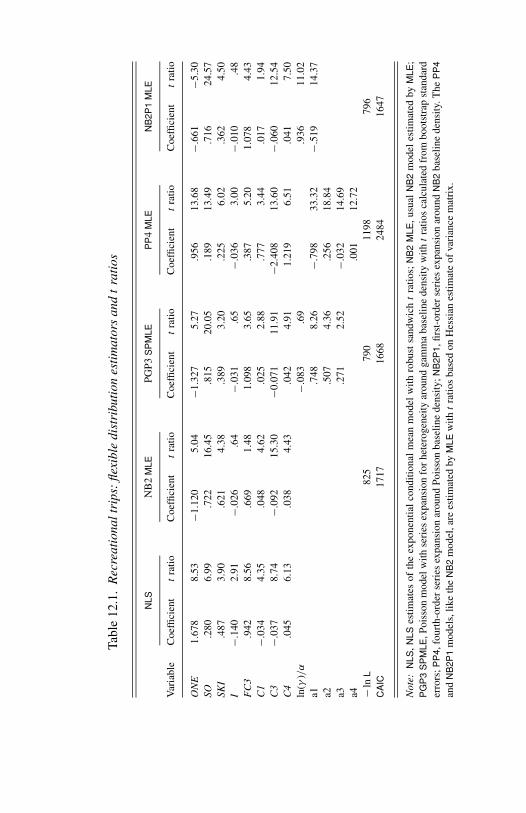
Tabl

e12

.1.

Rec

reat

iona

ltri

ps:

flexi

ble

dist

ribu

tion

esti

mat

ors

and

tra

tios

NLS

NB

2M

LEPG

P3S

PM

LEP

P4

MLE

NB

2P1

MLE

Var

iabl

eC

oeffi

cien

tt

ratio

Coe

ffici

ent

tra

tioC

oeffi

cien

tt

ratio

Coe

ffici

ent

tra

tioC

oeffi

cien

tt

ratio

ON

E1.

678

8.53

−1.1

205.

04−1

.327

5.27

.956

13.6

8−.

661

−5.3

0SO

.280

6.99

.722

16.4

5.8

1520

.05

.189

13.4

9.7

1624

.57

SKI

.487

3.90

.621

4.38

.389

3.20

.225

6.02

.362

4.50

I−.

140

2.91

−.02

6.6

4−.

031

.65

−.03

63.

00−.

010

.48

FC

3.9

428.

56.6

691.

481.

098

3.65

.387

5.20

1.07

84.

43C

1−.

034

4.35

.048

4.62

.025

2.88

.777

3.44

.017

1.94

C3

−.03

78.

74−.

092

15.3

0−0

.071

11.9

1−2

.408

13.6

0−.

060

12.5

4C

4.0

456.

13.0

384.

43.0

424.

911.

219

6.51

.041

7.50

ln(γ

)/α

−.08

3.6

9.9

3611

.02

a1.7

488.

26−.

798

33.3

2−.

519

14.3

7a2

.507

4.36

.256

18.8

4a3

.271

2.52

−.03

214

.69

a4.0

0112

.72

−ln

L82

579

011

9879

6C

AIC

1717

1668

2484

1647

Not

e:N

LS,N

LSes

timat

esof

the

expo

nent

ial

cond

ition

alm

ean

mod

elw

ithro

bust

sand

wic

ht

ratio

s;N

B2

MLE

,usu

alN

B2

mod

eles

timat

edby

MLE

;P

GP

3S

PM

LE,P

oiss

onm

odel

with

seri

esex

pans

ion

for

hete

roge

neity

arou

ndga

mm

aba

selin

ede

nsity

with

tra

tios

calc

ulat

edfr

ombo

otst

rap

stan

dard

erro

rs; P

P4,

four

th-o

rder

seri

esex

pans

ion

arou

ndPo

isso

nba

selin

ede

nsity

;NB

2P1,

first

-ord

erse

ries

expa

nsio

nar

ound

NB

2ba

selin

ede

nsity

.The

PP

4an

dN

B2P

1m

odel

s,lik

eth

eN

B2

mod

el,a

rees

timat

edby

MLE

with

tra

tios

base

don

Hes

sian

estim

ate

ofva

rian

cem

atri

x.

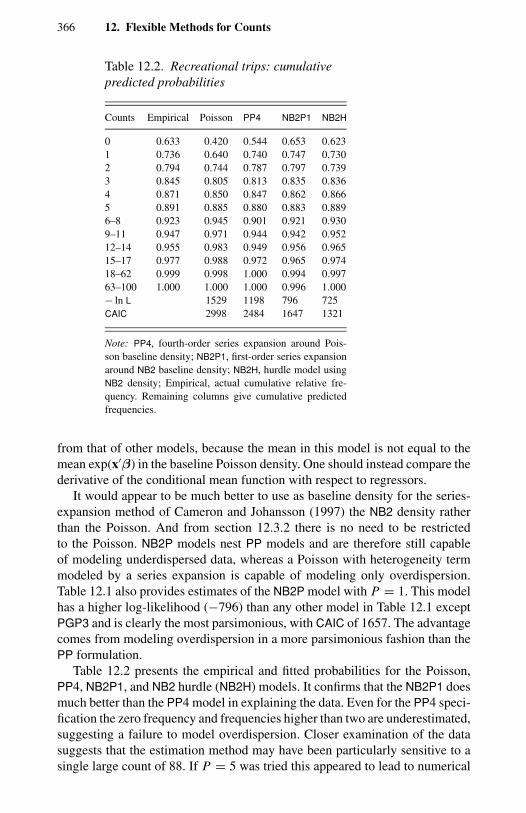
366 12. Flexible Methods for Counts

Table 12.2. Recreational trips: cumulativepredicted probabilities

Counts Empirical Poisson PP4 NB2P1 NB2H

0 0.633 0.420 0.544 0.653 0.6231 0.736 0.640 0.740 0.747 0.7302 0.794 0.744 0.787 0.797 0.7393 0.845 0.805 0.813 0.835 0.8364 0.871 0.850 0.847 0.862 0.8665 0.891 0.885 0.880 0.883 0.8896–8 0.923 0.945 0.901 0.921 0.9309–11 0.947 0.971 0.944 0.942 0.95212–14 0.955 0.983 0.949 0.956 0.96515–17 0.977 0.988 0.972 0.965 0.97418–62 0.999 0.998 1.000 0.994 0.99763–100 1.000 1.000 1.000 0.996 1.000− ln L 1529 1198 796 725CAIC 2998 2484 1647 1321

Note: PP4, fourth-order series expansion around Pois-son baseline density; NB2P1, first-order series expansionaround NB2 baseline density; NB2H, hurdle model usingNB2 density; Empirical, actual cumulative relative fre-quency. Remaining columns give cumulative predictedfrequencies.

from that of other models, because the mean in this model is not equal to themean exp(x′β) in the baseline Poisson density. One should instead compare thederivative of the conditional mean function with respect to regressors.

It would appear to be much better to use as baseline density for the series-expansion method of Cameron and Johansson (1997) the NB2 density ratherthan the Poisson. And from section 12.3.2 there is no need to be restrictedto the Poisson. NB2P models nest PP models and are therefore still capableof modeling underdispersed data, whereas a Poisson with heterogeneity termmodeled by a series expansion is capable of modeling only overdispersion.Table 12.1 also provides estimates of the NB2P model with P = 1. This modelhas a higher log-likelihood (−796) than any other model in Table 12.1 exceptPGP3 and is clearly the most parsimonious, with CAIC of 1657. The advantagecomes from modeling overdispersion in a more parsimonious fashion than thePP formulation.

Table 12.2 presents the empirical and fitted probabilities for the Poisson,PP4, NB2P1, and NB2 hurdle (NB2H) models. It confirms that the NB2P1 doesmuch better than the PP4 model in explaining the data. Even for the PP4 speci-fication the zero frequency and frequencies higher than two are underestimated,suggesting a failure to model overdispersion. Closer examination of the datasuggests that the estimation method may have been particularly sensitive to asingle large count of 88. If P = 5 was tried this appeared to lead to numerical

12.7. Derivations 367

instability, not surprising because 885 is a large number relative to most othersin the sample.

From Table 12.2 the NB2P1 is outperformed by the NB2H, even using CAIC,which penalizes the NB2H model for its additional parameters. We also com-pared the SPMLE results with those obtained by applying the constrained andunconstrained versions of the FMNB2 model, introduced in section 6.4. Theseare not reported in detail to save space. The chi-square goodness-of-fit testsrejected both variants of this model and confirmed that NB2H was the preferredmodel overall. It appears that for this data a hurdle specification is needed.

12.7 Derivations

We derive the section 12.2 result on optimal GMM for NB2 first four moments.For notational simplicity we drop the subscript i in (12.14). From (12.4), γ1σ

3 =σ 2(1 + 2αµ) and γ2σ

4 = σ 2 + 6ασ 4 + 3σ 4. Then

(σ 4γ2 − σ 4) − (1 + 2αµ)γ1σ3 = σ 4γ2 − σ 4 − (σγ1)γ1σ

3

= σ 4γ2 − σ 4 − σ 4γ 21

= σ 4γ2 − 1 − γ 2

1

,

σ 3γ1 − (1 + 2αµ)σ 2 = σ 2(1 + 2αµ) − (1 + 2αµ)σ 2

= 0,

and

σ 6(γ2 − 1 − γ 2

1

)= σ 2(σ 2 + 6ασ 4 + 3σ 4) − σ 6 − σ 4(1 + 2αµ)2

= σ 41 + 6ασ 2 + 2σ 2 − (1 + 2αµ)2= σ 41 + 6αµ(1 + αµ) + 2µ(1 + αµ)

− (1 + 4αµ + 4α2µ2)= σ 42(1 + α)µ(1 + αµ)= 2(1 + α)σ 6.

This yields (12.15).

12.8 Count Models: Retrospect and Prospect

In this concluding section we provide a brief retrospective look at the contentsand attempt to present a glimpse into possible future developments.

This book opens with reference to the vast statistical literature on iid uni-variate count distributions. A major thrust of the work of the recent decadeshas been to translate and extend analysis of counts to more general regressionmodels. Hence, most of the book is devoted to regression models for counts ina variety of data situations, including cross-section, time series, and panels.

Parametric count models are especially useful if the response variable takesrelatively few values and the counts are small. In most cases there is an advantage

368 12. Flexible Methods for Counts

in working with the exponential mean specification. It is important that theinherent heteroskedasticity of count data be modeled, an effective parsimoniousapproach being to specify the variance as a function of the mean. We haveemphasized parametric models based on discrete distributions, although modelsbased on discretization of a latent continuous distribution, such as the orderedprobit model, may also be used.

Count models are dual to waiting time models. The latter are often moreattractive and may well be more suitable for structural (as opposed to reducedform) modeling. In general, however, they require more data and may alsocall for more complex estimation procedures. Although analyzing counts in-stead may lead to information loss, it can still be informative about the role ofcovariates.

Significant additional complications arise from the presence of unobservedheterogeneity, truncation, censoring, joint dependence, measurement errors,and nonrandom sampling. These complications, generally studied extensivelyin the linear setting but less so for nonlinear models, have also been consideredin detail here. A variety of parametric and semiparametric estimators have beenpresented.

Use of flexible functional forms for the density and moments of count modelshas also been given considerable attention. These developments are practicallysignificant in many areas in which large heterogenous samples are available.

In the future we expect considerable emphasis to be given to applicationof computationally intensive methods to counts. At the most basic level thisincludes more widespread use of bootstrap methods and nonparametric andsemiparametric regression methods in simple cross-section settings.

At the frontier we expect this to lead to models that better accommodate em-pirical realities that are currently underdeveloped in certain areas. For example,the available estimation and inference procedures for multivariate counts, mod-els for nonrandom samples, and measurement errors are largely restricted tospecial models. Sometimes to handle one specific complication, others are sup-pressed. The simultaneous presence of several complications often results inmodels that may be conveniently analyzed by numerical methods only. Thislack of an analytical solution is increasingly becoming less of a barrier.

In dealing with models with a flexible representation of heterogeneity, insection 4.9, for example, it is shown why the Monte Carlo simulation approach isan attractive estimation strategy. Additional examples of this approach are citedin discussion of measurement error and selection bias models. The potentialfor application of such methods also is indicated in the context of maximumlikelihood estimation of multivariate models. This arises because the kernel ofthe likelihood is often an integral that must be numerically evaluated. Bayesiananalyses of these models typically share this feature also.

These examples appear to us as harbingers of an emerging new generation ofreduced form and structural models, exploiting advances in simulation-basedestimation that are already penetrating other areas of econometrics and statistics.

12.9. Bibliographic Notes 369

12.9 Bibliographic Notes

Optimal GMM in a variety of settings is covered in Newey (1993). Johnson,Kotz, and Kemp (1992, pp. 70–77) provide an informative account of the powerseries family of distributions. The articles by Cameron and Johansson (1997)and Gurmu et al. (1998) provide additional details on the computational aspectsof their respective estimators. For the generalized additive models approach toflexible specification of the conditional mean, Hastie and Tibshirani (1990) isan authoritative reference, and a good guide to the relevant software is Hilbe(1993). Applied aspects of nonparametric regression are dealt with in Hardle(1990). A relatively nontechnical introduction to kernel and nearest-neighbornonparametric regression is given by Altman (1992). A recent survey of regres-sion methods is given by Hardle and Linton (1994).

APPENDIX A

Notation and Acronyms

AIC: Akaike information criterionARMA: autoregressive moving averageBHHH: Berndt-Hall-Hall-Hausman algorithmBIC: Bayes information criterionBP: binary PoissonBoot: bootstrapCAIC: consistent Akaike information criterionCB: correlated binomialcdf: cumulative distribution functionCFMNB: slope-constrained finite mixture of negative binomialsCFMP: slope-constrained finite mixture of PoissonsCM: conditional moment (function or test)Cov: covarianceCP: correlated PoissonCV: coefficient of variationDARMA: discrete ARMAdgp: data generating processDiag: diagonalE: mathematical expectationEL: expected value of log-likelihood functionE[y | x]: conditional mean of y given xElast: elasticityEM: expectation-maximization (algorithm)f (y | x): conditional density of y given xFE: fixed effectsFMNB-C: C-component finite mixture of negative binomialFMP-C: C-component finite mixture of PoissonGEC(k): generalized event count modelGLM: generalized linear modelGLS: generalized least squaresGMM: generalized method of momentsiid: independently identically distributed

372 A. Notation and Acronyms

IM: information matrix (criterion or test)INAR: integer-valued autoregressive (model)INARMA: integer ARMAL[τ, z]: Laplace transformL: likelihood functionL: log-likelihood functionLEF: linear exponential familyLEFN: linear exponential family with nuisance parameterLM: Lagrange multiplierLR: likelihood ratiomgf: moment generating functionm(s; π1, . . . , πn): multinomial distributionM(t): moment generating functionMLE: maximum likelihood estimatorMLH: maximum likelihood HessianMLOP: maximum likelihood outer productMPSD: modified power series distributionN[µ, σ 2]: normal distribution with mean µ and variance σ 2

N[0, 1]: standard normal distributionNB: negative binomialNB1: NB distribution with linear variance functionNB2: NB distribution with quadratic variance functionNB1FE: negative binomial 1 fixed effects modelNBH: negative binomial hurdleNLIV: nonlinear instrumental variable (method)NLIV2: sequential two-step NLIVNLS: nonlinear least squaresNPML: nonparametric maximum likelihoodN(s, s + t): number of events observed in interval (s, s + t)OLS: ordinary (linear) least squaresOP: outer productOPG: outer product of the gradient (score) vectorsP[µ]: Poisson distribution with mean µ

pdf: probability density functionPFE: Poisson fixed effects (model)pgf: probability generating functionPGP: Poisson–gamma polynomial (model)PIG: Poisson inverse Gaussian mixturePML: pseudomaximum likelihoodPPp: polynomial Poisson (model) of order pPRE: Poisson random effects (model)PSD: power series distributionQEE: quadratic estimating equationQGPML: quasigeneralized PMLQGPMLE: QGPML estimator

A. Notation and Acronyms 373

QL: quasi likelihoodQVF: quadratic variance functionRE: random effectsRS: robust sandwich (variance estimator)SC: Schwarz Bayesian information criterionSPGLS: semiparametric generalized least squaresTCM: conditional moment test (statistic)TGoF: chi-square goodness-of-fit test (statistic)TH: Hausman test (statistic)TLR: likelihood ratio test (statistic)TLM: Lagrange multiplier (score) test (statistic)TW: Wald test (statistic)TZ: standard normal test (statistic)V: varianceV[y | x]: conditional variance of y given xWLS: weighted least squaresZIP: zero-inflated Poisson

APPENDIX B

Functions, Distributions, and Moments

For convenience we list in this appendix expressions and moment properties ofseveral univariate distributions that have been used in this book, most notablythe Poisson and negative binomial. But first we define the gamma function, acomponent of these distributions.

B.1 Gamma Function

Definition. The gamma function, denoted by (a), is defined by

(a) =∫ ∞

0e−t ta−1 dt, a > 0.

Properties of the gamma function include

1. (a) = (a − 1)(a − 1)2. (a) = (a − 1)! if a is a positive integer3. (0) = ∞, ( 1

2 ) = √π

4. (na) = (2π )(1−n)/2(n)na−1/2∏n−1k=0 (a + k

n ), where n is a positiveinteger.

Definition. The incomplete gamma function, denoted by γ (a, x), is defined by

γ (a, x) =∫ x

0e−t ta−1 dt ; a > 0, x > 0.

The ratio γ (a, x)/(a) is known as the incomplete gamma function ratio orthe gamma cdf.

The derivative of the logarithm of the gamma function is the digammafunction

d ln (a)

da= ψ(a).

The digamma function obeys the recurrence relation

ψ(a + 1) = ψ(a) + 1/a,

B.2. Some Distributions 375

and the j th derivative ψ ( j)(a +1) with respect to a obeys the recurrence relation

ψ ( j)(a + 1) = (−1) j j!a− j−1 + ψ ( j)(a).

B.2 Some Distributions

B.2.1 Poisson

The Poisson density for the count random variable y is

f (y) = e−µµy

y!; y = 0, 1, . . . ; µ > 0.

Then y ∼ P[µ] with mean µ, variance µ, moment generating function (mgf)exp [µ(et − 1)] and pgf exp [µ(t − 1)].

B.2.2 Logarithmic Series

The logarithmic series density for the positive valued count random variable yis

f (y) = αθ y

y; y = 1, 2, . . . ; 0 < θ < 1, α = −[log(1 − θ )]−1.

Then y has mean αθ/(1 − θ ), variance αθ (1 − αθ )/(1 − θ )2, mgf log(1 −θet )/ log(1 − θ ) and pgf log(1 − θ t)/ log(1 − θ ).

B.2.3 Negative Binomial

The negative binomial density for the count random variable y with parametersα and P is

f (y) =(

α + y − 1α − 1

)(P

1 + P

)y ( 1

1 + P

)α

;

y = 0, 1, . . . ; P, α > 0.

Then y has mean αP , variance αP(1 + P) and pgf (1 + P − Pt)−α .Different authors use different parameterizations of the negative binomial

(Johnson, Kotz, and Kemp, 1992). In this book we have used µ = αP , whichleads to

f (y) =(

α + y − 1α − 1

)(µ

α + µ

)y (α

α + µ

)α

,

which has mean µ and variance µ(1 + µ/α) and pgf (1 + µ/α − µt/α)−α .The special case of the geometric distribution is obtained by setting α = 1.

Pascal distribution is obtained by setting α equal to an integer.

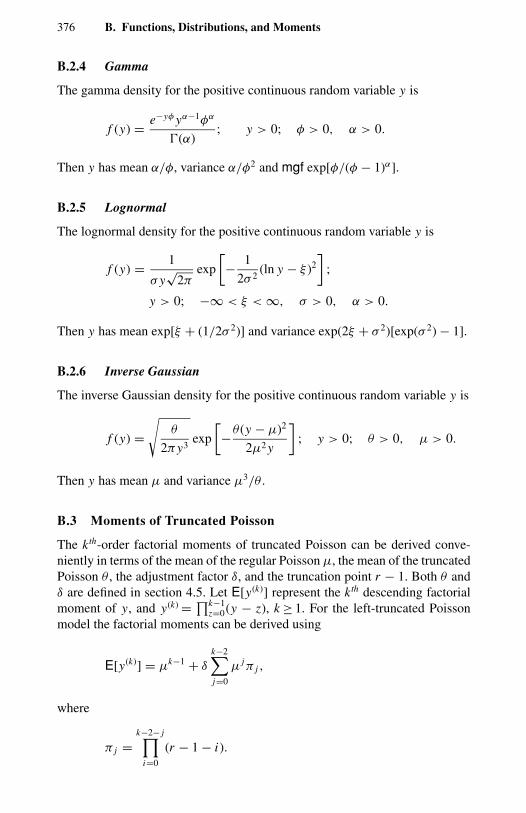
376 B. Functions, Distributions, and Moments

B.2.4 Gamma

The gamma density for the positive continuous random variable y is

f (y) = e−yφ yα−1φα

(α); y > 0; φ > 0, α > 0.

Then y has mean α/φ, variance α/φ2 and mgf exp[φ/(φ − 1)α].

B.2.5 Lognormal

The lognormal density for the positive continuous random variable y is

f (y) = 1

σ y√

2πexp

[− 1

2σ 2(ln y − ξ )2

];

y > 0; −∞ < ξ < ∞, σ > 0, α > 0.

Then y has mean exp[ξ + (1/2σ 2)] and variance exp(2ξ + σ 2)[exp(σ 2) − 1].

B.2.6 Inverse Gaussian

The inverse Gaussian density for the positive continuous random variable y is

f (y) =√

θ

2πy3exp

[−θ (y − µ)2

2µ2 y

]; y > 0; θ > 0, µ > 0.

Then y has mean µ and variance µ3/θ .

B.3 Moments of Truncated Poisson

The kth-order factorial moments of truncated Poisson can be derived conve-niently in terms of the mean of the regular Poisson µ, the mean of the truncatedPoisson θ , the adjustment factor δ, and the truncation point r − 1. Both θ andδ are defined in section 4.5. Let E[y(k)] represent the kth descending factorialmoment of y, and y(k) = ∏k−1

z=0(y − z), k ≥ 1. For the left-truncated Poissonmodel the factorial moments can be derived using

E[y(k)] = µk−1 + δ

k−2∑j=0

µ jπ j ,

where

π j =k−2− j∏

i=0

(r − 1 − i).

B.3. Moments of Truncated Poisson 377

Hence the first four factorial moments of the left-truncated Poisson are

E[y(1)] = θ

E[y(2)] = µθ + δ(r − 1)E[y(3)] = µ2θ + δ[(r − 1)(r − 2) + (r − 1)µ]E[y(4)] = µ3θ + δ[(r − 1)(r − 2)(r − 3)

+ (r − 1)(r − 2)µ + (r − 1)µ2].

Given the factorial moments, the uncentered and central moments can be ob-tained easily using the standard relationships between the three. For details seeGurmu and Trivedi (1992).

APPENDIX C

Software

Many widely used regression packages, including LIMDEP, STATA, TSP, andGAUSS, support maximum likelihood estimation of standard Poisson andnegative binomial regressions, the latter of these in a separate count mod-ule. LIMDEP also supports the QGPML versions of the standard models,maximum-likelihood estimation of truncated or censored Poisson, geometricand negative binomial models, and ZIP and sample selection models. STATAalso supports the generalized negative binomial regression in which the overdis-persion parameter is further parameterized as a function of additional covariates.In addition, any statistical package with a generalized linear models compo-nent will include maximum likelihood and QGPML estimation of the Poisson,although not necessarily negative binomial. Thus, regression packages coverthe models in Chapter 3 and roughly half of those in Chapter 4. The packagesvary somewhat in the provision of diagnostics such as overdispersion tests andgoodness-of-fit measures.

At the time of writing (late 1997) there is virtually no specialized software forthe models presented in Chapters 7 through 12. A notable exception is estima-tion of basic panel count data models, which is provided by both LIMDEP andTSP. For models for which off-the-shelf software is not available, one needs toprovide at least the likelihood function, for maximum likelihood estimation, orthe moment conditions and weighting matrix, for GMM estimation. In principlethis can be done using many regression packages, or using matrix programminglanguages such as GAUSS, MATLAB, S-PLUS, or SAS/IML. In practice nu-merical problems can be encountered if models are quite nonlinear. For muchof our work we have successfully used the MAXLIK optimization routinein GAUSS. Further information is available from accameron@ucdavis.edu ortrivedi@indiana.edu or http://www.econ.ucdavis.edu/count.html.

Software for simulation-based estimation is even less readily available. Tem-plate programs and algorithms may provide a useful starting point. For Markov-chain Monte Carlo methods a good reference to such resources is Gilks, Richard-son, and Spiegelhalter (1996). This work contains several articles on Bayesianestimation of mixtures using Gibbs sampling.

References

Aitchison, J., and C.H. Ho (1989), “The Multivariate Poisson-Log Normal Distribution,”Biometrika, 76, 643.

Aitkin, M., and D.B. Rubin (1985), “Estimation and Hypothesis Testing in Finite MixtureModels,” Journal of Royal Statistical Society B, 47, 67–75.

Akaike, H. (1973), “Information Theory and an Extension of the Maximum LikelihoodPrinciple,” in B.N. Petrov and F. Csaki, eds., Second International Symposium onInformation Theory, 267–281, Budapest, Akademiai Kaido.

Alcaniz, M. (1996), Modelos de Poisson Generalizados con una Variable de Exposicional Riesgo, Ph.D. dissertation, University of Barcelona, Spain.

Al-Osh, M.A., and A.A. Alzaid (1987), “First Order Integer Valued Autoregressive(INAR(1)) Process,” Journal of Time Series Analysis, 8, 261–275.

Altman, N.S. (1992), “An Introduction to Kernel and Nearest-Neighbor NonparametricRegression,” American Statistician, 46, 175–185.

Alzaid, A.A., and M.A. Al-Osh (1988), “First-Order Integer-Valued Autoregressive(INAR(1)) Process: Distributional and Regression Properties,” Statistica Neer-landica, 42, 53–61.

Alzaid, A.A., and M.A. Al-Osh (1990), “An Integer-Valued pth-Order AutoregressiveStructure (INAR(p)) Process,” Journal of Applied Probability, 27, 314–324.

Alzaid, A.A., and M.A. Al-Osh (1993), “Some Autoregressive Moving Average Pro-cesses with Generalized Poisson Distributions,” Annals of the Institute of Mathe-matical Statistics, 45, 223–232.

Amemiya, T. (1974), “The Nonlinear Two-Stage Least Squares Estimator,” Journal ofEconometrics, 2, 105–110.

Amemiya, T. (1984), “Tobit Models: A Survey,” Journal of Econometrics, 24, 3–61.Amemiya, T. (1985), Advanced Econometrics, Cambridge, MA, Harvard University

Press.Andersen, E.B. (1970), “Asymptotic Properties of Conditional Maximum Likelihood

Estimators,” Journal of the Royal Statistical Society B, 32, 283–301.Andersen, P.K., O. Borgan, R.D. Gill, and N. Keiding (1993), Statistical Models based

on Counting Processes, New York, Springer-Verlag.Andrews, D.W.K. (1988a), “Chi-Square Diagnostic Tests for Econometric Models:

Theory,” Econometrica, 56, 1419–1453.Andrews, D.W.K. (1988b), “Chi-Square Diagnostic Tests for Econometric Models:

Introduction and Applications,” Journal of Econometrics, 37, 135–156.

380 References

Arellano, M., and S. Bond (1991), “Some Tests of Specification for Panel Data: MonteCarlo Evidence and an Application to Employment Equations,” Review of EconomicStudies, 58, 277–298.

Arnold, B.C., and D.J. Strauss (1988), “Bivariate Distributions with Exponential Con-ditionals,” Journal of the American Statistical Association, 83, 522–527.

Arnold, B.C., and D.J. Strauss (1992), “Bivariate Distributions with Conditionals inPrescribed Exponential Families,” Journal of the Royal Statistical Society B, 53,365–375.

Australian Bureau of Statistics (1978), Australian Health Survey 1977–78 [machine-readable file], Australian Bureau of Statistics, Canberra.

Baltagi, B.H. (1995), Econometric Analysis of Panel Data, Chichester, UK, JohnWiley.

Barlow, R.E., and F. Proschan (1965), Mathematical Theory of Reliability, New York,John Wiley.

Barmby, T.A., C. Orme, and J.G. Treble (1991), “Worker Absenteeism: An AnalysisUsing Micro Data,” Economic Journal, 101, 214–229.

Berndt, E., B. Hall, R. Hall, and J. Hausman (1974), “Estimation and Inference inNonlinear Structural Models,” Annals of Economic and Social Measurement, 3/4,653–665.

Bishop, Y.M.M., S.E. Feinberg, and P.W. Holland (1975), Discrete Multivariate Analy-sis: Theory and Practice, Cambridge, MA, MIT Press.

Blonigen, B. (1997), “Firm-Specific Assets and the Link between Exchange Rates andForeign Direct Investment,” American Economic Review, 87, 447–465.

Blundell, R., R. Griffith, and J. Van Reenan (1995a), “Dynamic Count Models of Tech-nological Innovation,” Economic Journal, 105, 333–344.

Blundell, R., R. Griffith, and J. Van Reenan (1995b), “Market Share, Market Value andInnovation in a Panel of British Manufacturing Firms,” Discussion Paper 95-19,Department of Economics, University College London.

Blundell, R., R. Griffith, and F. Windmeijer (1995), “Individual Effects and Dynamicsin Count Data,” Discussion Paper 95-03, Department of Economics, UniversityCollege London.

Bohning, D. (1995), “A Review of Reliable Maximum Likelihood Algorithms for Semi-parametric Mixture Models,” Journal of Statistical Planning and Inference, 47,5–28.

Bohning, D., E. Dietz, R. Schaub, P. Schlattmann, and B.G. Lindsay (1994), “The Dis-tribution of the Likelihood Ratio for Mixtures of Densities from the One-Parame-ter Exponential Family,” Annals of the Institute of Statistical Mathematics, 46,373–388.

Bortkiewicz, L. von (1898), Das Gesetz de Kleinen Zahlen, Leipzig, Teubner.Boswell, M.T., and G.P. Patil (1970), “Chance Mechanisms Generating the Negative Bi-

nomial Distributions,” in G.P. Patil, ed., Random Counts in Models and Structures,volume 1, 3–22, University Park, PA, and London, Pennsylvania State UniversityPress.

Bourlange, D., and C. Doz (1988), “Pseudo-maximum de Vraisemblance: Experiencesde Simulations dans le Cadre d’un Modele de Poisson” (Pseudo Maximum Like-lihood Estimators: Monte-Carlo Experimentation in the Case of a Poisson Model[with English summary]), Annales d’Economie et de Statisques, 10, 139–176.

Brannas, K. (1992), “Limited Dependent Poisson Regression,” The Statistician, 41,413–423.

References 381

Brannas, K. (1994), “Estimation and Testing in Integer Valued AR(1) Models,” UmeaEconomic Studies No. 355, University of Umea.

Brannas, K. (1995a), “Explanatory Variables in the AR(1) Model,” Umea EconomicStudies No. 381, University of Umea.

Brannas, K. (1995b), “Prediction and Control for a Time Series Count Data Model,”International Journal of Forecasting, 11, 263–270.

Brannas, K. (1996), “Count Data Modelling: Measurement Errors in Exposure Time,”Umea Economic Studies No. 423, University of Umea.

Brannas, K., and P. Johansson (1992), “Estimation and Testing in a Model with SeriallyCorrelated Count Data,” in E. von Collani and R. Gob, eds., Proceedings of theSecond Wurzburg-Unea Conference in Statistics, University of Wurzburg.

Brannas, K., and P. Johansson (1994), “Time Series Count Regression,” Communicationsin Statistics: Theory and Methods, 23, 2907–2925.

Brannas, K., and P. Johansson (1996), “Panel Data Regression for Counts,” StatisticalPapers, 37, 191–213.

Brannas, K., and G. Rosenqvist (1994), “Semiparametric Estimation of HeterogeneousCount Data Models,” European Journal of Operations Research, 76, 247–258.

Breslow, N. (1990), “Tests of Hypotheses in Overdispersed Poisson Regression andOther Quasi-likelihood Models,” Journal of American Statistical Association, 85,565–571.

Breusch, T.S., and A.R. Pagan (1979), “A Simple Test for Heteroscedasticity,” Econo-metrica, 47, 1287–1294.

Browning, M. (1992), “Children and Household Economic Behavior,” Journal of Eco-nomic Literature, 30, 1434–1475.

Burguette, J., A.R. Gallant, and G. Souza (1982), “On the Unification of the AsymptoticTheory of Nonlinear Econometric Methods,” Econometric Reviews, 1, 151–190.

Cameron, A.C. (1991), “Regression Based Tests of Heteroskedasticity in Models Wherethe Variance Depends on the Mean,” Economics Working Paper Series No. 379,University of California, Davis.

Cameron, A.C., and P. Johansson (1997), “Count Data Regressions Using Series Ex-pansions with Applications,” Journal of Applied Econometrics, 12, 3, 203–224.

Cameron, A.C., and L. Leon (1993), “Markov Regression Models for Time Series Data,”presented at Western Economic Association Meetings, Lake Tahoe, NV.

Cameron, A.C., and P.K. Trivedi (1985), “Regression-based Tests for Overdispersion,”Econometric Workshop Technical Report No. 9, Stanford University.

Cameron, A.C., and P.K. Trivedi (1986), “Econometric Models Based on Count Data:Comparisons and Applications of Some Estimators,” Journal of Applied Econo-metrics, 1, 29–53.

Cameron, A.C., and P.K. Trivedi (1990a), “Regression-based Tests for Overdispersionin the Poisson Model,” Journal of Econometrics, 46, 347–364.

Cameron, A.C., and P.K. Trivedi (1990b), “Conditional Moment Tests and Orthogo-nal Polynomials,” Indiana University, Department of Economics, Working Paper90-051.

Cameron, A.C., and P.K. Trivedi (1990c), “Conditional Moment Tests with ExplicitAlternatives,” Economics Working Paper Series No. 366, University of California,Davis.

Cameron, A.C., and P.K. Trivedi (1990d), “The Information Matrix Test and Its ImpliedAlternative Hypotheses,” Economics Working Paper Series No. 372, University ofCalifornia, Davis.

382 References

Cameron, A.C., and P.K. Trivedi (1993), “Tests of Independence in Parametric Models:With Applications and Illustrations,” Journal of Business and Economic Statistics,11, 29–43.

Cameron, A.C., and P.K. Trivedi (1996), “Count Data Models for Financial Data,” inG.S. Maddala and C.R. Rao, eds., Handbook of Statistics, Volume 14, StatisticalMethods in Finance, Amsterdam, North-Holland.

Cameron, A.C., P.K. Trivedi, F. Milne, and J. Piggott (1988), “A MicroeconometricModel of the Demand for Health Care and Health Insurance in Australia,” Reviewof Economic Studies, 55, 85–106.

Cameron, A.C., and F.A.G. Windmeijer (1996), “R-Squared Measures for Count DataRegression Models with Applications to Health Care Utilization,” Journal of Busi-ness and Economic Statistics, 14, 209–220.

Cameron, A.C., and F.A.G. Windmeijer (1997), “An R-squared Measure of Goodness ofFit for Some Common Nonlinear Regression Models,” Journal of Econometrics,77, 329–342.

Campbell, M.J. (1994), “Time Series Regression for Counts: An Investigation into theRelationship between Sudden Infant Death Syndrome and Environmental Temper-ature,” Journal of the Royal Statistical Society A, 157, 191–208.

Carroll, R.J., D. Ruppert, and L.A. Stefanski (1995), Measurement Error in NonlinearModels, London, Chapman and Hall.

Chamberlain, G. (1987), “Asymptotic Efficiency in Estimation with Conditional MomentRestrictions,” Journal of Econometrics, 34, 305–334.

Chamberlain, G. (1992a), “Efficiency Bounds for Semiparametric Regression,” Econo-metrica, 60, 567–596.

Chamberlain, G. (1992b), “Comment: Sequential Moment Restrictions in Panel Data,”Journal of Business and Economic Statistics, 10, 20–26.

Chen, T.T. (1979), “Log-linear Models for Categorical Data with Misclassification andDouble Sampling,” Journal of the American Statistical Association, 74, 481–488.

Chesher, A. (1984), “Testing for Neglected Heterogeneity,” Econometrica, 52, 865–872.Chesher, A. (1991), “The Effect of Measurement Error,” Biometrika, 78, 451–462.Chesher, A., and M. Irish (1987), “Residual Analysis in the Grouped and Censored

Normal Linear Model,” Journal of Econometrics, 34, 33–62.Chib, S., E. Greenberg, and R. Winkelmann (1998), “Posterior Simulation and Bayes

Factors in Panel Count Data Models,” Journal of Econometrics, in press.Christmann, A. (1994), “Least Median of Weighted Squares in Logistic Regression with

Large Strata,” Biometrika, 81, 413–417.Christmann, A. (1996), “On Outliers and Robust Estimation in Regression Models with

Discrete Response Variables,” paper presented at Workshop on Statistical Mod-elling of Discrete Data and Structures, Sonderforschungbereich 386, University ofMunich.

Cincera, M. (1997), “Patents, R&D and Technological Spillovers at the Firm Level: SomeEvidence from Econometric Count Models for Panel Data,” Journal of AppliedEconometrics, 12, 265–280.

Cochran, W.G. (1940), “The Analysis of Variance When Experimental Errors Followthe Poisson or Binomial Law,” Annals of Mathematical Statistics, 11, 335–347.

Cohen, A.C. (1960), “Estimation in a Truncated Poisson Distribution When Zeros andOnes Are Missing,” Journal of the American Statistical Association, 55, 342–348.

Collings, B.J., and B.H. Margolin (1985), “Testing Goodness of Fit for the PoissonAssumption When Observations Are Not Identically Distributed,” Journal of theAmerican Statistical Association, 80, 411–418.

References 383

Conniffe, D.C. (1990), “Testing Hypotheses with Estimated Scores,” Biometrika, 77,97–106.

Consul, P.C. (1989), Generalized Poisson Distributions: Properties and Applications,New York, Marcel Dekker.

Consul, P.C., and F. Famoye (1992), “Generalized Poisson Regression Model,” Com-munications in Statistics: Theory and Method, 21, 89–109.

Consul, P.C., and G.C. Jain (1973), “A Generalization of the Poisson Distribution,”Technometrics, 15, 791–799.

Consul, P.C., and L.R. Shenton (1972), “Use of Lagrange Expansion for GeneratingDiscrete Generalized Probability Distributions,” SIAM Journal of Applied Mathe-matics, 23, 239–248.

Cox, D.R. (1955), “Some Statistical Models Related with Series of Events,” Journal ofthe Royal Statistical Society B, 17, 129–164.

Cox, D.R. (1961), “Tests of Separate Families of Hypotheses,” in Proceedings of theFourth Berkeley Symposium on Mathematical Statistics and Probability, 105–123.Berkeley, University of California Press.

Cox, D.R. (1962a), “Further Results on Tests of Separate Families of Hypotheses,”Journal of the Royal Statistical Society B, 24, 406–424.

Cox, D.R. (1962b), Renewal Theory, London, Methuen.Cox, D.R. (1981), “Statistical Analysis of Time Series: Some Recent Developments,”

Scandinavian Journal of Statistics, 8, 93–115.Cox, D.R. (1983), “Some Remarks on Overdispersion,” Biometrika, 70, 269–274.Cox, D.R., and P.A.W. Lewis (1966), The Statistical Analysis of Series of Events,

London, Methuen and Co.Cox, D.R., and E.J. Snell (1968), “A General Definition of Residuals [with discussion],”

Journal of the Royal Statistical Society B, 30, 248–275.Cragg, J.G. (1971), “Some Statistical Models for Limited Dependent Variables with

Application to the Demand for Durable Goods,” Econometrica, 39, 829–844.Cramer, H. (1946), Mathematical Methods of Statistics, Princeton, NJ, Princeton

University Press.Creel, M.D., and J.B. Loomis (1990), “Theoretical and Empirical Advantages of Trun-

cated Count Data Estimators for Analysis of Deer Hunting in California,” Journalof Agricultural Economics, 72, 434–441.

Crepon, B., and E. Duguet (1997a), “Estimating the Innovation Function fromPatent Numbers: GMM on Count Data,” Journal of Applied Econometrics, 12,243–264.

Crepon, B., and E. Duguet (1997b), “Research and Development, Competition and Inno-vation: Pseudo-maximum Likelihood and Simulated Maximum Likelihood MethodApplied to Count Data Models with Heterogeneity,” Journal of Econometrics, 79,355–378.

Crowder, M.J. (1976), “Maximum Likelihood Estimation for Dependent Observations,”Journal of the Royal Statistical Society B, 38, 45–53.

Crowder, M.J. (1987), “On Linear and Quadratic Estimating Functions,” Biometrika,74, 591–597.

Daley, D.J., and D. Vere-Jones (1988), An Introduction to the Theory of Point Processes,New York, Springer-Verlag.

Davidson, R., and J.G. MacKinnon (1981), “Several Tests for Model Specification inthe Presence of Alternative Hypotheses,” Econometrica, 49, 781–793.

Davidson, R., and J.G. MacKinnon (1993), Estimation and Inference in Econometrics,Oxford, Oxford University Press.

384 References

Davison, A.C., and A. Gigli (1989), “Deviance Residuals and Normal Scores Plots,”Biometrika, 76, 211–221.

Davison, A.C., and E.J. Snell (1991), “Residuals and Diagnostics,” in D.V. Hinkley,N. Reid, and E.J. Snell, eds., Statistical Theory and Modelling: In Honor of SirDavid Cox, FRS, 83–106, London, Chapman and Hall.

Davutyan, N. (1989), “Bank Failures as Poisson Variates,” Economic Letters, 29,333–338.

Dean, C. (1991), “Estimating Equations for Mixed Poisson Models,” in V.P. Godambe,ed., Estimating Functions, Oxford, Oxford University Press.

Dean, C. (1992), “Testing for Overdispersion in Poisson and Binomial Regression Mod-els,” Journal of the American Statistical Association, 87, 451–457.

Dean, C.B. (1993), “A Robust Property of Pseudo Likelihood Estimation for CountData,” Journal of Statistical Planning and Inference, 35, 309.

Dean, C.B. (1994), “Modified Pseudo-likelihood Estimator of the Overdispersion Pa-rameter in Poisson Mixture Models,” Journal of Applied Statistics, 1994, 21, 523.

Dean, C.B., and R. Balshaw (1997), “Efficiency Lost by Analyzing Counts Rather ThanEvent Times in Poisson and Overdispersed Poisson Regression Models,” Journalof the American Statistical Society, 92, 1387–1398.

Dean, C.B., D.M. Eaves, and C.J. Martinez (1995), “A Comment on the Use of EmpiricalCovariance Matrices in the Analysis of Count Data,” Journal of Statistical Planningand Inference, 48, 197–206.

Dean, C., and F. Lawless (1989a), “Tests for Detecting Overdispersion in Poisson Re-gression Models,” Journal of the American Statistical Association, 84, 467–472.

Dean, C., and J.F. Lawless (1989b), “Comment on Godambe and Thompson,” Journalof Statistical Planning and Inference, 22, 155–158.

Dean, C., J.F. Lawless, and G.E. Willmot (1989), “A Mixed Poisson-Inverse GaussianRegression Model,” Canadian Journal of Statistics, 17, 171–182.

Deb, P., and P.K. Trivedi (1997), “Demand for Medical Care by the Elderly: A FiniteMixture Approach,” Journal of Applied Econometrics, 12, 313–326.

Delgado, M.A. (1992), “Semiparametric Generalized Least Squares in the MultivariateNonlinear Regression Model,” Econometric Theory, 8, 203–222.

Delgado, M.A., and T.J. Kniesner (1997), “Count Data Models with Variance of Un-known Form: An Application to a Hedonic Model of Worker Absenteeism,” Reviewof Economics and Statistics, 79, 41–49.

Diggle, P.J., K-Y Liang, and S.L. Zeger (1994), Analysis of Longitudinal Data, Oxford,Clarendon Press.

Dionne, G., M. Artis, and M. Guillen (1996), “Count Data Models for a Credit ScoringSystem,” Journal of Empirical Finance, 3, 303–325.

Dionne, G., D. Desjardins, C. Labergue-Nadeau, and U. Maag (1995), “Medical Condi-tions, Risk Exposure, and Truck Drivers’ Accidents: An Analysis with Count DataRegression Models,” Accident Analysis and Prevention, 27, 295–305.

Dionne, G., and C. Vanasse (1992), “Automobile Insurance Rate Making in the Presenceof Asymmetrical Information,” Journal of Applied Econometrics, 7, 149–165.

Duan, N. (1983), “Smearing Estimate: A Nonparametric Retransformation Method,”Journal of the American Statistical Association, 78, 605–610.

Durbin, J. (1954), “Errors in Variables,” Review of the International Statistical Institute,22, 23–32.

Durbin, J., and S.J. Koopman (1997), “Monte Carlo Maximum Likelihood Estimationfor non-Gaussian State Space Models,” Biometrika, 84, 669–684.

References 385

Eagleson, G.K. (1964), “Polynomial Expansions of Bivariate Distributions,” Annals ofMathematical Statistics, 35, 1208–1215.

Eagleson, G.K. (1969), “A Characterization Theorem for Positive Definite Sequenceson the Krawtchouk Polynomials,” Australian Journal of Statistics, 11, 29–38.

Efron, B. (1979), “Bootstrapping Methods: Another Look at the Jackknife,” Annals ofStatistics, 7, 1–26.

Efron, B. (1986), “Double Exponential Families and Their Use in Generalized LinearRegressions,” Journal of the American Statistical Association, 81, 709–721.

Efron, B., and R.J. Tibshirani (1993), An Introduction to the Bootstrap, London, Chap-man and Hall.

Eggenberger, F., and G. Polya (1923), “Uber die Statistik Verketteter Vorgange,”Zeitschrift fur Angerwandte Mathematik and Mechanik (Journal of Applied Mathe-matics and Mechanics), 1, 279–289.

Eicker, F. (1967), “Limit Theorems for Regressions with Unequal and Dependent Er-rors,” in L. LeCam and J. Neyman, eds., Proceedings of the Fifth Berkeley Sympo-sium on Mathematical Statistics and Probability, 59–82, Berkeley, University ofCalifornia Press.

Englin, J., and J.S. Shonkwiler (1995), “Estimating Social Welfare Using Count DataModels: An Application to Long-Run Recreation Demand Under Conditions ofEndogenous Stratification and Truncation,” Review of Economics and Statistics,77, 104–112.

Everitt, B.S., and D.J. Hand (1981), Finite Mixture Distributions, London, Chapmanand Hall.

Fahrmeier, L., and H. Kaufman (1987), “Regression Models for Non-stationary Cate-gorical Time Series,” Journal of Time Series Analysis, 8, 147–160.

Fahrmeier, L., and G.T. Tutz (1994), Multivariate Statistical Modelling Based on Gen-eralized Linear Models, New York, Springer-Verlag.

Fan, J. (1992), “Design-Adaptive Nonparametric Regression,” Journal of the AmericanStatistical Association, 87, 998–1004.

Feinstein, J.S. (1989), “The Safety Regulation of U.S. Nuclear Power Plants: Viola-tions, Inspections, and Abnormal Occurrences,” Journal of Political Economy, 97,115–154.

Feinstein, J.S. (1990), “Detection Controlled Estimation,” Journal of Law and Eco-nomics, 33, 233–276.

Feller, W. (1943), “On a General Class of ‘Contagious’ Distributions,” Annals of Math-ematical Statistics, 14, 389–400.

Feller, W. (1968), An Introduction to Probability Theory and Its Applications, volume1, edition 3, New York, John Wiley.

Feller, W. (1971), An Introduction to Probability Theory, volume 2, New York, JohnWiley.

Feng, Z.D., and C.E. McCulloch (1996), “Using Bootstrap Likelihood Ratios in FiniteMixture Models,” Journal of the Royal Statistical Society B, 58, 609–617.

Fienberg, S.E. (1981), “Deciding What and Whom to Count,” in R.G. Lehnan and W.G.Skogan, eds., The NCS Working Papers, volume 1, U.S. Department of Justice.

Firth, D. (1987), “On the Efficiency of Quasi-likelihood Estimation,” Biometrika, 74,223–245.

Firth, D. (1991), “Generalized Linear Models,” in D.V. Hinkley, N. Reid, and E.J. Snell,eds., Statistical Theory and Modelling: In Honor of Sir David Cox, FRS, 55–82,London, Chapman and Hall.

386 References

Fleming, T.R., and D.P. Harrington (1991), Counting Process and Survival Analysis,New York, John Wiley.

Gallant, A.R., and D.W. Nychka (1987), “Seminonparametric Maximum LikelihoodEstimation,” Econometrica, 55, 363–390.

Gallant, A.R., and G. Tauchen (1989), “Seminonparametric Estimation of ConditionallyConstrained Heterogeneous Processes: Asset Pricing Applications,” Econometrica,57, 1091–1120.

Gauthier, G., and A. Latour (1994), “Convergence Forte des Estimateurs des Parametresd’un Processus GENAR(p),” Les Annales des sciences mathematics du Quebec,(with extended English abstract) forthcoming.

Geil, P., A. Melion, R. Rotte, and K.F. Zimmermann (1997), “Economic Incentives andHospitalization,” Journal of Applied Econometrics, 12, 295–311.

Gelfand, A.E., and S.R. Dalal (1990), “A Note on Overdispersed Exponential Families,”Biometrika, 77, 55–64.

Gilks, W.R., S. Richardson, and D.J. Spiegelhalter (1996), Markov Chain Monte Carloin Practice, London, Chapman and Hall.

Godambe, V.P., and M.E. Thompson (1989), “An Extension of Quasi-Likelihood Esti-mation,” Journal of Statistical Planning and Inference, 22, 137–152.

Goffe, W.L., Ferrier, G.D., and J. Rogers (1994), “Global Optimization of StatisticalFunctions with Simulated Annealing,” Journal of Econometrics, 60, 65–99.

Goldstein, H. (1995), Multilevel Statistical Models, edition 2, London, Edward Arnold.Good, D., and M.A. Pirog-Good (1989), “Models for Bivariate Count Data with an

Application to Teenage Delinquency and Paternity,” Sociological Methods andResearch, 17, 409–431.

Gourieroux, C., and A. Monfort (1991), “Simulation Based Inference in Models withHeterogeneity,” Annales D’Economie Et De Statistique, 20/21, 70–107.

Gourieroux, C., and A. Monfort (1995), Statistics and Econometrics Models, volumes 1and 2, translated by Q. Vuong, Cambridge, Cambridge University Press. (Originallypublished as Statistique et modeles econometriques, 1989).

Gourieroux, C., and A. Monfort (1997), Simulation Based Econometric Methods,Oxford, Oxford University Press.

Gourieroux, C., A. Monfort, and A. Trognon (1984a), “Pseudo Maximum LikelihoodMethods: Theory,” Econometrica, 52, 681–700.

Gourieroux, C., A. Monfort, and A. Trognon (1984b), “Pseudo Maximum LikelihoodMethods: Applications to Poisson Models,” Econometrica, 52, 701–720.

Gourieroux, C., A. Monfort, E. Renault, and A. Trognon (1987a), “Generalized Resid-uals,” Journal of Econometrics, 34, 5–32.

Gourieroux, C., A. Monfort, E. Renault, and A. Trognon (1987b), “Simulated Residuals,”Journal of Econometrics, 34, 201–252.

Gourieroux, C., and M. Visser (1997), “A Count Data Model with Unobserved Hetero-geneity,” Journal of Econometrics, 79, 247–268.

Greene, W.H. (1994), “Accounting for Excess of Zeros and Sample Selection in Poissonand Negative Binomial Regression Models,” Discussion Paper EC-94-10, Depart-ment of Economics, New York University.

Greene, W.H. (1997a), Econometric Analysis, edition 3, New York, MacMillan.Greene, W.H. (1997b), “FIML Estimation of Sample Selection Models for Count Data,”

Discussion Paper EC-97-02, Department of Economics, Stern School of Business,New York University.

References 387

Greenwood, M., and G.U. Yule (1920), “An Inquiry into the Nature of Frequency Dis-tributions of Multiple Happenings, with Particular Reference to the Occurrence ofMultiple Attacks of Disease or Repeated Accidents,” Journal of the Royal StatisticalSociety A, 83, 255–279.

Grogger, J. (1990), “The Deterrent Effect of Capital Punishment: An Analysis of DailyHomicide Counts,” Journal of the American Statistical Association, 85, 295–303.

Grogger, J.T., and R.T. Carson (1991), “Models for Truncated Counts,” Journal of Ap-plied Econometrics, 6, 225–238.

Gupta, C.R. (1974), “Modified Power Series Distribution and Some of its Applications,”Sankhya, Series B, 36, 288–298.

Gurmu, S. (1991), “Tests for Detecting Overdispersion in the Positive Poisson Regres-sion Model,” Journal of Business and Economic Statistics, 9, 215–222.

Gurmu, S. (1993), “Testing for Overdispersion in Censored Poisson Regression Models,”Discussion Paper 255, The Jefferson Center for Political Economy, University ofVirginia.

Gurmu, S. (1997), “Semiparametric Estimation of Hurdle Regression Models withan Application to Medicaid Utilization,” Journal of Applied Econometrics, 12,225–242.

Gurmu, S., P. Rilstone, and S. Stern (1995), “Nonparametric Hazard Rate Estimation,”Department of Economics, Discussion Paper, University of Virginia.

Gurmu, S., P. Rilstone, and S. Stern (1998), “Semiparametric Estimation of CountRegression Models,” forthcoming Journal of Econometrics.

Gurmu, S., and P.K. Trivedi (1992), “Overdispersion Tests for Truncated Poisson Re-gression Models,” Journal of Econometrics, 54, 347–370.

Gurmu, S., and P.K. Trivedi (1993), “Variable Augmentation Specification Tests in theExponential Family,” Econometric Theory, 9, 94–113.

Gurmu, S., and P.K. Trivedi (1994), “Recent Developments in Models of Event Counts:A Survey,” Discussion Paper 261, The Jefferson Center for Political Economy,University of Virginia.

Gurmu, S., and P.K. Trivedi (1996), “Excess Zeros in Count Models for RecreationalTrips,” Journal of Business and Economic Statistics, 14, 469–477.

Haab, T.C., and K.E. McConnell (1996), “Count Data Models and the Problem of Zerosin Reaction Demand Analysis,” American Journal of Agricultural Economics, 78,89–98.

Haight, F. A. (1967), Handbook of the Poisson Distribution, New York, John Wiley.Hall, A. (1987), “The Information Matrix Test in the Linear Model,” Review of Economic

Studies, 54, 257–265.Hall, B.H., Griliches, Z., and J.A. Hausman (1986), “Patents and R and D: Is There a

Lag?,” International Economic Review, 27, 265–283.Hamilton, J.D. (1989), “A New Approach to the Economic Analysis of Nonstationary

Time Series and the Business Cycle,” Econometrica, 57, 357–384.Hamilton, J.D. (1994), Time Series Analysis, Princeton, NJ, Princeton University Press.Hannan, M.T., and J. Freeman (1987), “The Ecology of Organizational Founding: Amer-

ican Labor Unions, 1836–1985,” American Journal of Sociology, 92, 910–943.Hansen, L.P. (1982), “Large Sample Properties of Generalized Method of Moments

Estimators,” Econometrica, 50, 1029–1054.Hardle, W. (1990), Applied Nonparametric Methods, Cambridge, UK, Cambridge

University Press.

388 References

Hardle, W., and O. Linton (1994), “Applied Nonparametric Methods,” in R.F. Engle andD. McFadden, eds., Handbook of Econometrics, volume 4, Amsterdam, North–Holland.

Harvey, A.C. (1989), Forecasting, Structural Time Series Models and the Kalman Filter,Cambridge, UK, Cambridge University Press.

Harvey, A.C., and C. Fernandes (1989), “Time Series Models for Count or QualitativeObservations [with discussion],” Journal of Business and Economic Statistics, 7,407–417.

Harvey, A.C., and N. Shephard (1993), “Stuctural Time Series Models,” in G.S. Maddala,C.R. Rao, and H.D. Vinod, eds., Handbook of Statistics, Volume 11, Econometrics,Amsterdam, North–Holland.

Harville, D. (1977), “Maximum Likelihood Estimation of Variance Componentsand Related Problems,” Journal of the American Statistical Association, 72,320–340.

Hastie, T.J., and R.J. Tibshirani (1990), Generalized Additive Models, New York, Chap-man and Hall.

Hausman, J.A. (1978), “Specification Tests in Econometrics,” Econometrica, 46, 1251–1271.

Hausman, J.A., B.H. Hall, and Z. Griliches (1984), “Econometric Models for CountData with an Application to the Patents–R and D Relationship,” Econometrica, 52,909–938.

Hausman, J.A., G.K. Leonard, and D. McFadden (1995), “A Utility-Consistent, Com-bined Discrete Choice and Count Data Model: Assessing Recreational Use Lossesdue to Natural Resource Damage,” Journal of Public Economics, 56, 1–30.

Hausman, J.A., A.W. Lo, and A.C. MacKinlay (1992), “An Ordered Probit Analysis ofTransaction Stock Prices,” Journal of Financial Economics, 31, 319–379.

Heckman, J. J. (1976), “The Common Structure of Statistical Models of Truncation,Sample Selection, and Limited Dependent Variables and a Simple Estimator forSuch Models,” Annals of Economics and Social Measurement, 5, 475–492.

Heckman, J.J. (1984), “The χ2 Goodness of Fit Test for Models with Parameters Esti-mated from Micro Data,” Econometrica, 52, 1543–1547.

Heckman, J., and B. Singer (1984), “A Method of Minimizing the Impact of Distribu-tional Assumptions in Econometric Models for Duration Data,” Econometrica, 52,271–320.

Hendry, D. F. (1995), Dynamic Econometrics, Oxford, Oxford University Press.Hilbe, J. M. (1993), “Generalized Additive Models Software,” American Statistician,

47, 59–64.Hill, S., D. Rothchild, and A.C. Cameron (1998), “Tactical Information and the Diffu-

sion of Peaceful Protests,” in D.A. Lake and D. Rothchild, eds., The InternationalSpread of Ethnic Conflict: Fear, Diffusion, and Escalation, Princeton, NJ, PrincetonUniversity Press.

Hinde, J. (1982), “Compound Poisson Regression Models,” in R. Gilchrist, ed., GLIM82: Proceedings of the International Conference on Generalised Linear Models,New York, Springer-Verlag.

Holly, A. (1982), “A Remark on Hausman’s Specification Test,” Econometrica, 50,749–759.

Holly, A. (1987), “Specification Tests: An Overview,” in T.F. Bewley, ed., Advances inEconomics and Econometrics: Theory and Applications, volume 1, Fifth WorldCongress, 59–97, Cambridge, UK, Cambridge University Press.

References 389

Honda, Y. (1988), “A Size Correction to the Lagrange Multiplier Test for Heteroskedas-ticity,” Journal of Econometrics, 38, 375–386.

Horowitz, J.L. (1997), “Bootstrap Methods in Econometrics: Theory and Numeri-cal Performance,” in D.M. Kreps and K.F. Wallis, eds., Advances in Economicsand Econometrics: Theory and Applications, volume 3, Seventh World Congress,Cambridge, UK, Cambridge University Press.

Hsiao, C. (1986), Analysis of Panel Data, Cambridge, UK, Cambridge University Press.Huber, P.J. (1967), “The Behavior of Maximum Likelihood Estimates under Nonstandard

Conditions,” in L. LeCam and J. Neyman, eds., Proceedings of the Fifth BerkeleySymposium on Mathematical Statistics and Probability, 221–234, Berkeley, Uni-versity of California Press.

Imbens, G.W., and T. Lancaster (1994), “Combining Micro and Macro Data in Microe-conometric Models,” Review of Economic Studies, 61, 655–680.

Jacobs, P.A., and P.A.W. Lewis (1977), “A Mixed Autoregressive Moving AverageExponential Sequence and Point Process,” Advances in Applied Probability, 9,87–104.

Jacobs, P.A., and P.A.W. Lewis (1978a), “Discrete Time Series Generated by Mixtures I:Correlational and Runs Properties,” Journal of the Royal Statistical Society B, 40,94–105.

Jacobs, P.A., and P.A.W. Lewis (1978b), “Discrete Time Series Generated by Mixtures II:Asymptotic Properties,” Journal of the Royal Statistical Society B, 40, 222–228.

Jacobs, P.A., and P.A.W. Lewis (1983), “Stationary Discrete Autoregressive MovingAverage Time Series Generated by Mixtures,” Journal of Time Series Analysis, 4,19–36.

Jaggia, S. (1991), “Specification Tests Based on the Generalized Gamma Model ofDuration – With an Application to Kennan Strike Data,” Journal of Applied Econo-metrics, 6, 169–180.

Jaggia, S., and S. Thosar (1993), “Multiple Bids as a Consequence of Target Manage-ment Resistance: A Count Data Approach,” Review of Quantitative Finance andAccounting, 3, 447–457.

Jewel, N. (1982), “Mixtures of Exponential Distribuhtions,” Annals of Statistics, 10,479–484.

Jin-Guan, D., and L. Yuan (1991), “The Integer-Valued Autoregressive (INAR(p))Model,” Journal of Time Series Analysis, 12, 129–142.

Johansson, P. (1995), “Tests for Serial Correlation and Overdispersion in a CountData Regression Model,” Journal of Statistical Computation and Simulation, 53,153–164.

Johansson, P. (1996), “Speed Limitation and Motorway Casualties: A Time Series CountData Regression Approach,” Accident Analysis and Prevention, 28, 73–87.

Johansson, P., and M. Palme (1996), “Do Economics Incentives Affect Work Absence:Empirical Evidence Using Swedish Micro Data,” Journal of Public Economics, 59,195–218.

Johnson, N.L., and S. Kotz (1969), Discrete Distributions, Boston, Houghton Mifflin.Johnson, N.L., S. Kotz, and N. Balakrishnan (1994), Continuous Univariate Distribu-

tions, edition 2, New York, John Wiley.Johnson, N.L., S. Kotz, and N. Balakrishnan (1997), Discrete Multivariate Distributions,

New York, John Wiley.Johnson, N.L., S. Kotz, and A.W. Kemp (1992), Univariate Distributions, edition 2,

New York, John Wiley.

390 References

Johnston, J., and J. DiNardo (1997), Econometric Methods, edition 4, New York,McGraw-Hill.

Jordan, P., D. Brubacher, S. Tsugane, Y. Tsubono, K.F. Gey, and U. Moser (1997),“Modeling Mortality Data from a Multi-Center Study in Japan by Means of PoissonRegression with Errors in Variables,” International Journal of Epidemiology, 26,501–507.

Jorgensen, B. (1987), “Exponential Dispersion Models [with discussion]”, Journal ofthe Royal Statistical Society B, 49, 127–162.

Jorgensen, B. (1997), The Theory of Dispersion Models, London, Chapman and Hall.Jorgenson, D.W. (1961), “Multiple Regression Analysis of a Poisson Process,” Journal

of the American Statistical Association, 56, 235–245.Jung, C.J., and R. Winkelmann (1993), “Two Apects of Labor Mobility: A Bivariate

Poisson Regression Approach,” Empirical Economics, 18, 543–556.Jupp, P.E., and K.V. Mardia (1980), “A General Correlation Coefficient for Directional

Data and Related Regression Problems,” Biometrika, 67, 163–173.Kalbfleisch, J.D., and R.L. Prentice (1980), The Statistical Analysis of Failure Time

Data, New York, Wiley.Katz, L. (1963), “Unified Treatment of a Broad Class of Discrete Probability Distribu-

tions,” in G.P. Patil, ed., Classical and Contagious Discrete Distributions, Calcutta,Statistical Publishing Society.

Keane, M.P., and D.E. Runkle (1992), “On the Estimation of Panel-Data Models withSerial Correlation When Instruments Are Not Strictly Exogenous,” Journal of Busi-ness and Economic Statistics, 10, 1–9.

Kennan, J. (1985), “The Duration of Contract Strikes in U.S. Manufacturing,” Journalof Econometrics, 28, 5–28.

Kianifard, F., and P.P. Gallo (1995), “Poisson Regression Analysis in Clinical Research,”Journal of Biopharmaceutical Statistics, 5, 115–129.

King, G. (1987a), “Presidential Appointments to the Supreme Court: Adding System-atic Explanation to Probabilistic Description,” American Political Quarterly, 15,373–386.

King, G. (1987b), “Event Count Models for International Relations: Generalizationsand Applications,” International Studies Quarterly, 33, 123–147.

King, G. (1989a), “A Seemingly Unrelated Poisson Regression Model,” SociologicalMethods and Research, 17, 235–255.

King, G. (1989b), “Variance Specification in Event Count Models: From RestrictiveAssumptions to a Generalized Estimator,” American Journal of Political Science,33, 762–784.

Kingman, J.F.C. (1993), Poisson Processes, Oxford, Oxford University Press.Kocherlakota, S., and K. Kocherlakota (1993), Bivariate Discrete Distributions, New

York, Marcel Dekker.Koenker, R. (1982), “A Note on Studentizing a Test for Heteroskedasticity,” Journal of

Econometrics, 17, 107–112.Kotz, S., and N.L. Johnson (1982–89), Encyclopedia of Statistical Sciences, vol. 1–9,

New York, John Wiley.Laird, N. (1978), “Nonparametric Maximum Likelihood Estimation of a Mixing Distri-

bution,” Journal of the American Statistical Association, 73, 805–811.Lambert, D. (1992), “Zero-Inflated Poisson Regression with an Application to Defects

in Manufacturing,” Technometrics, 34, 1–14.

References 391

Lancaster, H.O. (1969), The Chi-squared Distribution, New York, John Wiley.Lancaster, T. (1984), “The Covariance Matrix of the Information Matrix Test,” Econo-

metrica, 52, 1051–1054.Lancaster, T. (1990), The Econometric Analysis of Transitional Data, New York, Cam-

bridge University Press.Landwehr, J.M., D. Pregibon, and A.C. Shoemaker (1984), “Graphical Methods for

Assessing Logistic Regression Models [with discussion],” Journal of the AmericanStatistical Association, 79, 61–83.

Lawless, J.F. (1987a), “Regression Methods for Poisson Process Data,” Journal of theAmerican Statistical Association, 82, 808–815.

Lawless, J.F. (1987b), “Negative Binomial and Mixed Poisson Regressions,” The Cana-dian Journal of Statistics, 15, 209–225.

Lawless, J.F. (1995), “The Analysis of Recurrent Events for Multiple Subjects,” AppliedStatistics: Journal of the Royal Statistical Society C, 44, 487–498.

Lee, L.-F. (1983), “Generalized Econometric Models with Selectivity,” Econometrica,51, 507–512.

Lee, L.-F. (1986), “Specification Test for Poisson Regression Models,” InternationalEconomic Review, 27, 689–706.

Lee, L.-F. (1997), “Specification and Estimation of Count Data Regression and SampleSelection Models: A Counting Process and Waiting Time Approach,” presentedat the North American Summer Meetings of the Econometric Society, Pasadena,CA.

Leon, L.F., and C.-L. Tsai (1998), “The Assessment of Model Adequacy for MarkovRegression Time Series Models,” forthcoming Biometrics.

Leroux, B.G. (1992), “Consistent Estimation of a Mixing Distribution,” Annals of Statis-tics, 20, 1350–1360.

Lewis, P.A.W. (1985), “Some Simple Models for Continuous Variate Time Series,” WaterResources Bulletin, 21, 635–644.

Li, W.K. (1991), “Testing Model Adequacy for Some Markov Regression Models forTime Series,” Biometrika, 78, 83–89.

Liang, K.-Y., and S. Zeger (1986), “Longitudinal Data Analysis Using GeneralizedLinear Models,” Biometrika, 73, 13–22.

Lindeboom, M., and G.J. van den Berg (1994), “Heterogeneity in Models for BivariateSurvival: The Importance of Mixing Distribution,” Journal of the Royal StatisticalSociety B, 56, 49–60.

Lindsay, B.G. (1995), Mixture Models: Theory, Geometry and Applications, NSF-CBMSRegional Conference Series in Probability and Statistics, volume 5, IMS-ASA.Hayward, CA: Institute of Mathematical Statistics.

Lindsay, B.G., and K. Roeder (1992), “Residual Diagnostics in the Mixture Model,”Journal of the American Statistical Association, 87, 785–795.

Liu, R.Y. (1988), “Bootstrap Procedures under Some Non-i.i.d. Models,” Annals ofStatistics, 16, 1696–1700.

Long, J.S. (1997), Regression Models for Categorical and Limited Dependent Variables,Thousand Oaks, CA, Sage Publications.

Lu, M.Z., and G.E. Mizon (1996), “The Encompassing Principle and Hypothesis Test-ing,” Econometric Theory, 12, 845–858.

Lucerno, A. (1995), “A Family of Partially Correlated Poisson Models for Overdisper-sion,” Computational Statistics and Data Analysis, 20, 511–520.

392 References

MacDonald, I.L., and W. Zucchini (1997), Hidden Markov and Other Models forDiscrete-Valued Time Series, London, Chapman and Hall.

Maddala, G.S. (1983), Limited Dependent and Qualitative Variables in Econometrics,Cambridge, Cambridge University Press.

Mammen, E. (1993), “Bootstrap and Wild Bootstrap for High Dimensional Linear Mod-els,” Annals of Statistics, 21, 255–285.

Manski, C.F. (1995), Identification Problems in the Social Sciences. Cambridge, MA,Harvard University Press.

Manski, C.F., and D. McFadden, eds. (1981), Structural Analysis of Discrete Data withEconometric Applications, Cambridge, MA, MIT Press.

Marshall, A.W., and I. Olkin (1990), “Multivariate Distributions Generated from Mix-tures of Convolution and Product Families,” in H.W. Block, A.R. Sampson, andT.H. Savits, eds., Topics in Statistical Dependence, IMS Lecture Notes MonographSeries, volume 16, 371–393. Hayward, CA, Institute of Mathematical Statistics.

Matyas, L., and P. Sevestre (1995), The Econometrics of Panel Data: A Handbookof the Theory with Applications, edition 3, Nordrecht, The Netherlands, KluwerAcademic Publishers.

Mayer, W.J., and W.F. Chappell (1992), “Determinants of Entry and Exit: An Applicationof Bivariate Compounded Poisson Distribution to U.S. Industries, 1972–1977,”Southern Economic Journal, 58, 770–778.

McCallum, J., C. Raymond, and C. McGilchrist (1995), “How Accurate Are Self Reportsof Doctor Visits? A Comparison Using Australian Health Insurance CommissionRecords,” National Center for Epidemiology and Population Health, The AustralianNational University.

McCullagh, P. (1983), “Quasi-likelihood Functions,” The Annals of Statistics, 11,59–67.

McCullagh, P. (1986), “The Conditional Distribution of Goodness-of-Fit Statistics forDiscrete Data,” Journal of the American Statistical Association, 81, 104–107.

McCullagh, P., and J.A. Nelder (1989, 1983), Generalized Linear Models, editions 1and 2, London, Chapman and Hall.

McFadden, D., and P. Ruud (1994), “Estimation by Simulation,” Review of Economicsand Statistics, 76, 591–608.

McGilchrist, C.A. (1994), “Estimation in Generalized Mixed Models,” Journal of theRoyal Statistical Society B, 56, 61–69.

McKenzie, E. (1985), “Some Simple Models for Discrete Variate Time Series,” WaterResources Bulletin, 21, 645–650.

McKenzie, E. (1986), “Autoregressive Moving-Average Processes with Negative Bino-mial and Geometric Marginal Distributions,” Advances in Applied Probability, 18,679–705.

McKenzie, E. (1988), “Some ARMA Models for Dependent Sequences of PoissonCounts,” Advances in Applied Probability, 22, 822–835.

McLachlan, G.J., and K.E. Basford, (1988), Mixture Models: Inference and Applicationto Clustering, New York, Marcel Dekker.

Meghir, C., and J.-M. Robin (1992), “Frequency of Purchase and Estimation of DemandEquations,” Journal of Econometrics, 53, 53–86.

Merkle, L., and K.F. Zimmermann (1992), “The Demographics of Labor Turnover:A Comparison of Ordinal Probit and Censored Count Data Models,” ReserchesEconomiques de Louvain, 58, 283–307.

References 393

Mizon, G.E., and J.-F. Richard (1986), “The Encompassing Principle and Its Applicationto Testing Non-nested Hypotheses,” Econometrica, 54, 657–678.

Montalvo, J.G. (1997), “GMM Estimation of Count-Panel-Data Models with Fixed Ef-fects and Predetermined Instruments,” Journal of Business and Economic Statistics,15, 82–89.

Moore, D.F. (1986), “Asymptotic Properties of Moment Estimators for OverdispersedCounts and Proportions,” Biometrika, 73, 583–588.

Moran, P.A.P. (1971), “Maximum Likelihood Estimation in Non-standard Conditions,”Proceedings of the Cambridge Philosophical Society, 70, 441–450.

Morrison, D.G., and D.C. Schmittlein (1988), “Generalizing the NBD Model for Cus-tomer Purchases: What Are the Implications and Is It Worth the Effort?,” Journalof Economics and Business Statistics, 6, 145–166.

Moschopoulos, P., and J.G. Staniswalis (1994), “Estimation Given Conditional from anExponential Family,” The American Statistician, 48, 271–275.

Mukhopadhyay, K., and P.K. Trivedi (1995), “Regression Models for Under-reportedCounts,” preprint. Paper presented at Econometric Society World Congress, Tokyo.

Mullahy, J. (1986), “Specification and Testing of Some Modified Count Data Models,”Journal of Econometrics, 33, 341–365.

Mullahy, J. (1997a), “Instrumental Variable Estimation of Poisson Regression Models:Application to Models of Cigarette Smoking Behavior,” Review of Economics andStatistics, 79, 586–593.

Mullahy, J. (1997b), “Heterogeneity, Excess Zeros and the Structure of Count DataModels,” Journal of Applied Econometrics, 12, 337–350.

Mundlak, Y. (1978), “On the Pooling of Time Series and Cross Section Data,” Econo-metrica, 46, 69–85.

Murphy, K., and R. Topel (1985), “Estimation and Inference in Two Step EconometricModels,” Journal of Business and Economic Statistics, 3, 370–379.

Nagin, D.S., and K.C. Land (1993), “Age, Criminal Careers and Population Heterogene-ity: Specification and Estimation of a Nonparametric, Mixed Regression Model,”Criminology, 31, 327–362.

National Medical Expenditure Survey (1987), National Center for Health Services Re-search and Health Care Technology, Rockville, Maryland.

Nelder, J.A., and D. Pregibon (1987), “An Extended Quasi-likelihood Function,”Biometrika, 74, 221–232.

Nelder, J.A., and R.W.M. Wedderburn (1972), “Generalized Linear Models,” Journal ofthe Royal Statistical Society A, 135, 370–384.

Newell, D.J. (1965), “Unusual Frequency Distributions,” Biometrics, 21, 159–168.Newey, W.K. (1984), “A Methods of Moments Interpretation of Sequential Estimators,”

Economics Letters, 14, 201–206.Newey, W.K. (1985), “Maximum Likelihood Specification Testing and Conditional Mo-

ment Tests,” Econometrica, 53, 1047–1070.Newey, W.K. (1990a), “Efficient Instrumental Variable Estimation of Nonlinear Mod-

els,” Econometrica, 58, 809–838.Newey, W. (1990b), “Semiparametric Efficiency Bounds,” Journal of Applied Econo-

metrics, 5, 99–136.Newey, W.K. (1993), “Efficient Estimation of Models with Conditional Moment Restric-

tions,” in G.S. Maddala, C.R. Rao, and H.D. Vinod, eds., Handbook of Statistics,Volume 11, Econometrics, 419–454, Amsterdam, North-Holland.

394 References

Newey, W.K., and D. McFadden (1994), “Large Sample Estimation and Hypothesis Test-ing,” in R.F. Engle and D. McFadden, eds., Handbook of Econometrics, volume 4,Amsterdam, North-Holland.

Newey, W.K., and K.D. West (1987a), “A Simple, Positive Semi-definite, Hetero-scedasticity and Autocorrelation Consistent Covariance Matrix,” Econometrica,55, 703–708.

Newey, W.K., and K.D. West (1987b), “Hypothesis Testing with Efficient Methods ofMoments Estimators,” International Economic Review, 28, 777–787.

Newhouse, J.P. (1993), Free for All? Lessons from the Rand Health Insurance Experi-ment. Cambridge, MA, Harvard University Press.

Neyman, J. (1939), “On a New Class of Contagious Distributions Applicable in Ento-mology and Bacteriology,” Annals of Mathematical Statistics, 10, 35–57.

Neyman, J. (1965), “Certain Chance Mechanisms Involving Discrete Distributions,” inG.N. Patil, ed., Classical and Contagious Discrete Distributions, 1–14, Calcutta,Statistical Publishing House.

Nickell, S. (1981), “Biases in Dynamic Models with Fixed Effects,” Econometrica, 49,1399–1416.

Noack, A. (1950), “A Class of Random Variables with Discrete Distributions,” Annalsof Mathematical Statistics, 21, 127–132.

Ogaki, M. (1993), “Generalized Method of Moments: Econometric Applications,” inG.C. Maddala, C.R.Rao, and H.D. Vinod, eds., Handbook of Statistics, Volume 11,Econometrics, Amsterdam, North-Holland.

Okoruwa, A.A., J.V. Terza, and H.O. Nourse (1988), “Estimating Patronization Sharesfor Urban Retail Centers: An Extension of the Poisson Gravity Model,”Journal ofUrban Economics, 24, 241–259.

Ozuna, T., and I. Gomaz (1995), “Specification and Testing of Count Data RecreationDemand Functions,” Empirical Economics, 20, 543–550.

Pagan, A.R. (1986), “ Two Stage and Related Estimators and Their Applications,” Reviewof Economic Studies, 53, 517–538.

Pagan, A., and F. Vella (1989), “Diagnostic Tests for Models Based on Individual Data:A Survey,” Journal of Applied Econometrics, 4, S29–S59.

Page, M. (1995), “Racial and Ethnic Discrimination in Urban Housing Markets: Evi-dence from a Recent Audit Survey,” Journal of Urban Economics, 38, 183–206.

Palmgren, J. (1981), “The Fisher Information Matrix for Log-Linear Models ArguingConditionally in the Observed Explanatory Variables,” Biometrika, 68, 563–566.

Patil, G.P. (1970), ed., Random Counts in Models and Structures, volumes 1–3, Univer-sity Park, PA, and London, Pennsylvania State University Press.

Patterson, H.D., and R. Thompson (1971), “Recovery of Inter-block Information WhenBlock Sizes Are Unequal,” Biometrika, 58, 545–554.

Pesaran, M.H. (1987), “Global and Partial Non-Nested Hypotheses and AsymptoticLocal Power,” Econometric Theory, 3, 677–694.

Phillips, P.C.B. (1987), “Time Series Regression with a Unit Root,” Econometrica, 55,277–301.

Pierce, D. (1982), “The Asymptotic Effect of Substituting Estimators for Parameters inCertain Types of Statistics,” Annals of Statistics, 10, 475–478.

Pierce, D.A., and D.W. Schafer (1986), “Residuals in Generalized Linear Models,”Journal of the American Statistical Association, 81, 977–986.

Pinquet, J. (1997), “Experience Rating through Heterogeneous Models,” Working PaperNo. 9725, THEMA, Universite Paris X-Nanterre.

References 395

Pohlmeier,W., and V. Ulrich (1995), “An Econometric Model of the Two-Part Decision-making Process in the Demand for Health Care,” Journal of Human Resources, 30,339–361.

Poisson, S.-D. (1837), Recherches sur la Probabilite des Jugements en Matiere Crim-inelle et en Matiere Civile, Paris, Bachelier.

Pope, A., J. Schwartz, and M. Ransom (1992), “Daily Mortality and PM10 Pollution inUtah Valley,” Archives of Environmental Health, 47, 211–217.

Pregibon, D. (1981), “Logistic Regression Diagnostics,” Annals of Statistics, 9, 705–724.Pudney, S. (1989), Modelling Individual Choice: The Econometrics of Corners, Kinks

and Holes, New York, Basil Blackwell.Qin, J., and J. Lawless (1994), “Empirical Likelihood and General Estimating Equa-

tions,” Annals of Statistics, 22, 300–325.Ramaswamy, V., E.N. Anderson, and W.S. DeSarbo (1994), “A Disaggregate Negative

Binomial Regression Procedure for Count Data Analysis,” Management Science,40, 405–417.

Robert, C.P. (1996), “Mixtures of Distributions: Inference and Estimation,” in W.R.Gilks, S. Richardson, and D.J. Spiegelhalter, eds., Markov Chain Monte Carlo inPractice, 441–464, London, Chapman and Hall.

Robinson, P.M. (1987), “Asymptotically Efficient Estimation in the Presence of Het-eroskedasticity of Unknown Form,” Econometrica, 55, 875–891.

Robinson, P.M. (1988), “Root-N Consistent Semiparametric Regression,” Economet-rica, 56, 931–954.

Ronning, G., and R.C. Jung (1992), “Estimation of a First Order Autoregressive Processwith Poisson Marginals for Count Data,” in L. Fahrmeir, et al., eds., Advances inGLIM and Statistical Modelling, New York, Springer-Verlag.

Rose, N. (1990), “Profitability and Product Quality: Economic Determinants of AirlineSafety Performance,” Journal of Political Economy, 98, 944–964.

Ross, S.M. (1996), Stochastic Processes, edition 2, New York, John Wiley.Ruser, J.W. (1991), “Workers’ Compensation and Occupational Injuries and Illnesses,”

Journal of Labor Economics, 9, 325–350.Sargan, J.D. (1958), “The Estimation of Economic Relationships using Instrumental

Variables,” Econometrica, 26, 393–415.Santos Silva, J.M.C. (1997), “Unobservables in Count Data Models for On-site Sam-

ples,” Economics Letters, 54, 217–220.Schall, R. (1991), “Estimation in Generalized Linear Models with Random Effects,”

Biometrika, 78, 719–727.Schmidt, P., and A. Witte (1989), “Predicting Criminal Recidivism Using Split-

population Survival Time Models,” Journal of Econometrics, 40, 141–159.Schneider, A.L. (1981), “Differences Between Survey and Police Information about

Crime,” in R.G. Lehnan and W.G. Skogan, eds., The NCS Working Papers, volume 1,U.S. Department of Justice.

Schwartz, E.S., and W.N. Torous (1993), “Mortgage Prepayments and Default Decisions:A Poisson Regression Approach,” AREUEA Journal: Journal of the American RealEstate Association, 21, 431–449.

Schwarz, G. (1978), “Estimating the Dimension of a Model,” Annals of Statistics, 6,461–464.

Sellar, C., J.R. Stoll, and J.P. Chavas (1985), “Validation of Empirical Measures ofWelfare Change: A Comparison of Nonmarket Techniques,” Land Economics, 61,156–175.

396 References

Severini, T.A., and J.G. Staniswalis (1994), “Quasi-likelihood Estimation in Semipara-metric Models,” Journal of American Statistical Association, 89, 501–511.

Shaban, S.A. (1988), “Poisson-Lognormal Distributions,” in E.L. Crow and K. Shimizu,eds., Lognormal Distributions, 195–210, New York, Marcel Dekker.

Shaked, M. (1980), “On Mixtures from Exponential Families,” Journal of Royal Statis-tical Society B, 42, 415–433.

Shaw, D. (1988), “On-Site Samples’ Regression Problems of Non-negative Integers,Truncation and Endogenous Stratification,” Journal of Econometrics, 37, 211–223.

Shephard, N. (1995), “Generalized Linear Autoregression,” Nuffield College, OxfordUniversity.

Shephard, N., and M.K. Pitt (1997), “Likelihood Analysis of Non-Gaussian Measure-ment Time Series,” Biometrika, 84, 653–667.

Shiba, T., and H. Tsurumi (1988), “Bayesian and Non-Bayesian Tests of Independence inSeemingly Unrelated Regressions,” International Economic Review, 29, 377–395.

Simar, L. (1976), “Maximum Likelihood Estimation of a Compound Poisson Process,”Annals of Statistics, 4, 1200–1209.

Singh, A.C., and G.R. Roberts (1992), “State Space Modelling of Cross-Classified TimeSeries of Counts,” International Statistical Review, 60, 321–335.

Smith, R.J. (1997), “Alternative Semi-parametric Likelihood Approaches to GeneralisedMethod of Moment Estimation,” Economic Journal, 107, 503–519.

Smyth, G.K. (1989), “Generalized Linear Models with Varying Dispersion,” Journal ofthe Royal Statistical Society B, 51, 47–60.

Solow, A. R. (1993), “Estimating Record Inclusion Probability,” American Statistician,47, 206–209.

Staniswalis, J. (1989), “The Kernel Estimate of a Regression Function in Likelihood-Based Models,” Journal of the American Statistical Association, 84, 426–431.

Steutel, F.W., and K. Van Harn (1979), “Discrete Analogues of Self-Decomposabilityand Stability, Annals of Probability, 7, 893–899.

Stroud, A.H., and D. Secrest (1966), Gaussian Quadrature Formulas, Englewood Cliffs,NJ, Prentice Hall.

Stukel, T. (1988), “Generalized Logistic Models,” Journal of the American StatisticalAssociation, 83, 426–431.

Szu, H., and R. Hartley (1987), “Fast Simulated Annealing,” Physics Letters A, 122,157–162.

Tauchen, G. (1985), “Diagnostic Testing and Evaluation of Maximum Likelihood Mod-els,” Journal of Econometrics, 30, 415–443.

Taylor, H.M., and S. Karlin (1994), An Introduction to Stochastic Modelling, revisededition, San Diego and New York, Academic Press.

Teicher, H. (1961), “The Identifiability of Mixtures,” Annals of Mathematical Statistics,32, 244–248.

Terza, J.V. (1985), “A Tobit-Type Estimator for the Censored Poisson RegressionModel,” Economics Letters, 18, 361–365.

Terza, J.V. (1998), “Estimating Count Data Models with Endogenous Switching: Sam-ple Selection and Endogenous Switching Effects,” Journal of Econometrics, 84,129–139.

Terza, J.V., and P.W. Wilson (1990), “Analyzing Frequencies of Several Types of Events:A Mixed Multinomial-Poisson Approach,” Review of Economics and Statistics, 72,108–115.

References 397

Thall, P.F., and S.C. Vail (1990), “Some Covariance Models for Longitudinal CountData with Overdispersion,” Biometrika, 46, 657–671.

Titterington, D.M., A.F. Smith, and U.E. Makov (1985), Statistical Analysis of FiniteMixture Distributions, Chichester, UK, John Wiley.

U.S. National Center for Health Statistics (1965), Health Interview Responses Comparedwith Medical Records, Vital and Health Statistics Series 2 No. 7 Public HealthService, Washington, U.S. Government Printing Office.

U.S. National Center for Health Statistics (1967), Interview Data on Chronic Condi-tions Compared with Information Derived from Medical Records, Vital and HealthStatistics Series 2 No. 23 Public Health Service, Washington, U.S. GovernmentPrinting Office.

Van Duijn, M.A.J., and U. Bockenholt (1995), “Mixture Models for the Analysis ofRepeated Count Data,” Applied Statistics: Journal of the Royal Statistical SocietyC, 44, 473–485.

van Praag, B.M.S., and E.M. Vermeulen (1993), “A Count-Amount Model with Endoge-nous Recording of Observations,” Journal of Applied Econometrics, 8, 383–395.

Vuong, Q.H. (1989), “Likelihood Ratio Tests for Model Selection and Non-nested Hy-pothesis,” Econometrica, 57, 307–333.

Wagner, G.G., R.V. Burkhauser, and F. Behringer (1993), “The English Language PublicUse File of The German Socio-Economic Panel,” Journal of Human Resources,28, 429–433.

Wang, P., I.M. Cockburn, and M.L. Puterman (1998). “Analysis of Patent Data – AMixed Poisson Regression Model Approach,” Journal of Business and EconomicStatistics, 16(1), 27–41.

Watermann, J., R. Jankowski, and I. Madan (1994), “Under-reporting of NeedlestickInjuries by Medical Students,” Journal of Hospital Infection, 26, 149–151.

Wedderburn, R.W.M. (1974), “Quasi-likelihood Functions, Generalized Linear Models,and the Gauss-Newton Method,” Biometrika, 61, 439–447.

Wedel, W., W.S. DeSarbo, J.R. Bult, and V. Ramaswamy (1993), “A Latent Class PoissonRegression Model for Heterogeneous Count Data,” Journal of Applied Economet-rics, 8, 397–411.

Weiss, A.A. (1995), “Simultaneity and Sample Selection in Poisson Regression Models,”unpublished discussion paper.

West, M., and P. J. Harrison (1997, 1990), Bayesian Forecasting and Dynamic Models,edition 2, New York, Springer.

West, M., P.J. Harrison, and H.S. Migon (1985), “Dynamic Generalized Linear Modelsand Bayesian Forecasting [with discussion],” Journal of the American StatisticalAssociation, 80, 73–97.

White, H. (1980), “A Heteroskedasticity-Consistent Covariance Matrix Estimator and aDirect Test for Heteroskedasticity,” Econometrica, 46, 817–838.

White, H. (1982), “Maximum Likelihood Estimation of Misspecified Models,” Econo-metrica, 50, 1–25.

White, H. (1994), Estimation, Inference, and Specification Analysis, Cambridge, UK,Cambridge University Press.

White, H., and I. Domowitz (1984), “Nonlinear Regression with Dependent Observa-tions,” Econometrica, 52, 143–161.

Whittemore, A.S., and G. Gong (1991), “Poisson Regression with Misclassified Counts:Application to Cervical Cancer Mortality Rates,” Applied Statistics, 40, 81–93.

398 References

Williams, D.A. (1987), “Generalized Linear Model Diagnostics Using the Deviance andSingle Case Deletions,” Applied Statistics, 36, 181–191.

Windmeijer, F.A.G., and J. M. C. Santos Silva (1997), “Endogeneity in Count Data Mod-els: An Application to Demand for Health Care,” Journal of Applied Econometrics,12, 281–294.

Winkelmann, R. (1997, 1994), Count Data Models: Econometric Theory and Applica-tion to Labor Mobility, Berlin, Springer-Verlag.

Winkelmann, R. (1995), “Duration Dependence and Dispersion in Count-Data Models,”Journal of Business and Economic Statistics, 13, 467–474.

Winkelmann, R., and K.F. Zimmermann (1991), “A New Approach for Modeling Eco-nomic Count Data,” Economics Letters, 37, 139–143.

Winkelmann, R., and K.F. Zimmermann (1992), “Recursive Probability Estimators forCount Data,” in G. Haag, U. Muller, and K.G. Troitzsch, eds., Economic Evolutionand Demographic Change, 321–329, New York, Springer.

Winkelmann, R., and K.F. Zimmermann (1993), “Poisson Logistic Regression,”SELAPO, University of Munich.

Winkelmann, R., and K.F. Zimmermann (1995), “Recent Developments in Count DataModelling: Theory and Application,” Journal of Economic Surveys, 9, 1–24.

Wong, W.H. (1986), “Theory of Partial Likelihood,” Annals of Statistics, 14, 88–123.Wooldridge, J.M. (1990a), “A Unified Approach to Robust, Regression-Based Specifi-

cation Tests,” Econometric Theory, 6, 17–43.Wooldridge, J.M. (1990b), “An Encompassing Approach to Conditional Mean Tests

with Applications to Testing Nonlinear Hypotheses,” Journal of Econometrics, 45,331–350.

Wooldridge, J.M. (1990c), “Distribution-Free Estimation of Some Nonlinear Panel DataModels,” Working Paper No. 564, Department of Economics, Massachusetts Insti-tute of Technology.

Wooldridge, J.M. (1991a), “On the Application of Robust, Regression-Based Diag-nostics to Models of Conditional Means and Conditional Variances,”Journal ofEconometrics, 47, 5–46.

Wooldridge, J.M. (1991b), “Specification Testing and Quasi-Maximum Likelihood Es-timation,” Journal of Econometrics, 48, 29–55.

Wooldridge, J.M. (1997), “Multiplicative Panel Data Models without the Strict Exo-geneity Assumption,” Econometric Theory, 13, 667–679.

Wu, D. (1973), “Alternative Tests of Independence between Stochastic Regressors andDisturbances,” Econometrica, 41, 733–750.

Yannaros, N. (1993), “Analyzing Incomplete Count Data,” Statistician, 42, 181–187.Zeger, S.L. (1988), “A Regression Model for Time Series of Counts,” Biometrika, 75,

621–629.Zeger, S.L., and K.-Y. Liang (1986), “Longitudinal Data Analysis for Discrete and

Continuous Outcomes,” Biometrics, 42, 121–130.Zeger, S.L., K.-Y. Liang, and P.S. Albert (1988), “Models for Longitudinal Data: A

Generalized Estimating Equation Approach,” Biometrics, 44, 1049–1060.Zeger, S.L., and Qaqish B. (1988), “Markov Regression Models for Time Series: A

Quasi-Likelihood Approach,” Biometrics, 44, 1019–1031.

Author Index

Aitchison, J., 273, 379Aitken, M., 130, 379Akaike, H., 182–3, 379Al-Osh, M. A., 236, 379Albert, P. S., 290, 398Alcaniz, M., 303, 324, 379Altman, N. S., 362, 369, 379Alzaid, A. A., 236, 379Amemiya, T., 41, 51, 57, 117, 137, 181, 326,

324, 332–3, 379Andersen, E. B., 7, 379Andersen, P. K., 282, 379Anderson, E. N., 220, 395Andrews, D. W. K., 157, 187, 198, 379Arellano, M., 294, 300, 380Arnold, B. C., 273, 380Artis, M., 18, 384

Balakrishnan, N., 273, 392, 389Balshaw, D., 8, 384Baltagi, B., 277, 294, 300, 380Barlow, R. E., 111, 380Barmby, T., 313, 380Basford, K. E., 128, 137, 392Beringer, F., 12, 397Berndt, E., 24, 380Bishop, Y. M. M., 153, 380Blonigen, B., 292, 380Blundell, R., 238, 283, 294, 297–8, 333–6, 380Bockenholt, U., 292, 397Bohning, D., 129, 132, 137, 197, 380Bond, M., 294, 300, 380Borgan, R. D., 7, 379Bortkiewicz, L., von 1, 11, 380Boswell, M. T., 102, 138, 380Bourlange, D., 106, 380Brannas, K., 137, 229, 234–8, 242, 244, 248,

250, 290, 294, 303, 380–1Breslow, N., 187, 381Breusch, T. S., 176, 381Browning, M., 332, 381Brubacher, D., 307, 390

Bult, J., 129, 397Burguette, J., 333, 381Burkhauser, R. V., 12, 397

Cameron, A. C., 12, 17, 29, 65, 68, 77, 94, 98,112, 154–5, 158, 161–2, 173, 175, 176,178, 180, 187, 219, 229, 240, 264–6, 268,295, 324, 326, 351, 353, 355, 364–6, 369,381, 382, 388

Campbell, M. J., 242, 382Carroll, R. J., 57, 301, 307, 324, 382Carson, R., 137, 219, 387Chamberlain, G., 42, 263, 273, 285, 296, 298,

382Chappell, W. F., 251, 273, 392Chavas, J. P., 207, 395Chen, T. T., 326, 382Chesher, A., 143–4, 179, 324, 382Chib, S., 289, 382Christmann, A., 312, 382Cincera, M., 298, 382Cochrane, W. G., 17, 382Cockburn, I. M., 220, 397Cohen, A. C., 322, 382Collings, B. J., 187, 382Conniffe, D. C., 168, 383Consul, P. C., 103, 116–7, 356, 383Cox, D. R., 98, 111, 142, 146, 158, 162–3,

182–3, 187, 225, 230, 250, 303, 305, 383Cragg, J., 124, 383Cramer, H., 264, 383Creel, M. D., 137, 383Crepon, B., 137, 294, 298, 383Crowder, M. J., 23, 345–7, 383

Dalal, S. R., 136, 197, 386Daley, D. J., 104, 383Davidson, R., 25, 47, 50–1, 57, 182, 383Davison, A. C., 145–6, 187, 384Davutyan, N., 13, 229, 384Dean, C. B., 8, 65, 103, 105, 111, 167–8, 187,

347, 384

400 Author Index

Deb, P., 137, 192–3, 206, 384Delgado, M. A., 263, 362–3, 384DeSarbo, W. S., 129, 220, 395, 397Desjardins, D., 306, 384Dietz, E., 197, 380Diggle, P. J., 277–8, 284, 289, 294, 300, 384DiNardo, J., 20, 390Dionne, G., 13, 18, 190, 219, 306, 324, 384Domowitz, I., 226, 397Doz, C., 106, 380Duan, N., 90, 384Duguet, E., 137, 294, 298, 383Durbin, J., 180, 244, 384

Eagleson, G. K., 315, 316, 324, 385Eaves, D. M., 65, 384Efron, B., 36, 114–5, 164–5, 167, 187, 385Eggenberger, F., 1, 102, 107, 385Eicker, F., 39, 66, 385Englin, J., 321, 331, 385Everitt, B. S., 128, 385

Fahrmeier, L., 57, 239–40, 250, 289, 291, 300,385

Famoye, F., 117, 383Fan, J., 145, 385Feinberg, S. E., 153, 380, 385Feinstein, J. S., 313, 318–9, 385Feller, W., 17, 102, 106–7, 136, 317, 385Feng, Z. D., 133, 218, 385Fernandes, C., 243–4, 388Ferrier, G. D., 354, 386Firth, D., 187, 347, 385Fleming, T. R., 7, 386Freeman, J., 18, 387

Gallant, A. R., 266, 333, 350–1, 381, 386Gallo, P. P., 94, 390Gauthier, G., 236, 386Geil, P., 193, 327, 386Gelfand, A. E., 136, 197, 386Gey, K. F., 307, 390Gigli, A., 145, 384Gilks, W. R., 378, 386Gill, R. D., 7, 379Godambe, V. P., 345, 347, 386Goffe, W. L., 354, 386Goldstein, H., 300, 386Gomaz, I., 12, 207–8, 394Gong, G., 302, 310–2, 397Good, D., 273, 386Gourieroux, C., 2, 29, 31–3, 36, 57, 94, 98,

123, 134–5, 137, 143–4, 181, 260, 340,386

Greenberg, E., 289, 382, 386Greene, W. H., 13, 20, 44, 94, 339–41, 386Greenwood, M., 1, 100, 107, 387Griffith, R., 238, 283, 294, 297–8, 333, 380

Griliches, Z., 2, 12, 16, 94, 283, 286, 288,291–4, 298, 387–8

Grogger, J. T., 18, 137, 219, 387Guillen, M., 18, 384Gupta, C. R., 355, 387Gurmu, S., 17, 95, 118, 120, 122, 137, 144,

160, 168, 193, 207, 219, 304, 351,359–62, 364, 369, 377, 387

Haab, T. C., 220, 387Haight, F. A., 17, 387Hall, A. R., 179, 387Hall, B. H., 2, 12, 16, 24, 94, 283, 286, 288–9,

291–4, 298, 380, 387–8Hall, R., 24, 380Hamilton, J., 57, 387Hand, D. J., 128, 385Hannan, M. T., 18, 387Hansen, L. P., 39, 41, 57, 333, 387Hardle, W., 369, 387, 388Harrington, D. P., 7, 386Harrison, P. J., 243, 250, 397Hartley, R., 354, 396Harvey, A. C., 243–4, 250, 388Harville, D., 278, 388Hastie, T. J., 358, 369, 388Hausman, J., 2, 12, 16, 24, 88, 94, 180–1, 252,

270–1, 283, 286, 288, 291–4, 298, 380,387–8

Heckman, J. J., 105, 129, 157, 196, 336, 388Hendry, D. F., 57, 253, 388Hilbe, J. M., 369, 388Hill, S., 295, 388Hinde, J., 135, 385, 388Ho, C. H., 273, 379Holland, P. W., 153, 380Holly, A., 181, 388Honda, Y., 168, 389Horowitz, J. L., 164, 167, 187, 389Hsiao, C., 377–8, 284, 290, 294, 300, 389Huber, P. J., 26, 39, 389

Imbens, G. W., 343, 389Irish, M., 143–4, 382

Jacobs, P. A., 234, 245, 389Jaggia, S., 13, 146, 231, 389Jain, G. C., 103, 383Jankowski, R., 313, 397Jewel, N., 104, 389Jin-Guan, D., 236, 389Johansson, P., 158, 219, 229, 242, 244, 266,

290, 294, 313, 351, 353–5, 364, 366, 369,381, 389

Johnson, N. L., 1, 17, 108, 117, 130, 257, 273,342, 356, 369, 375, 389, 390

Johnston, J., 20, 390Jordan, P., 307, 390

Author Index 401

Jorgensen, B., 36, 115, 390Jorgenson, D. W., 17, 94, 390Jung, C. J., 236, 258, 273, 390, 395Jupp, P. E., 258, 268, 390

Kalbfleisch, J. D., 109, 390Karlin, S., 3, 6, 17, 390, 396Katz, L., 112, 390Kaufman, H., 239, 385, 390Keane, M. P., 300, 390Keiding, N., 7, 379, 390Kemp, A., 1, 17, 103, 130, 356, 369, 375, 389,

390Kennan, J., 231, 390Kianifard, F., 94, 390King, G., 14, 18, 90, 112, 258, 273, 390Kingman, J. F. C., 4, 5, 15, 17, 98, 136, 390Kniesner, T. J., 362–3, 384Kocherlakota, K., 256, 258, 272–3, 390Kocherlakota, S., 256, 258, 272–3, 390Koenker, R., 172, 390Koopman, S., 244, 384Kotz, S., 1, 17, 103, 117, 130, 257, 273, 342,

356, 369, 375, 389–90

Labergue-Nadeau, C., 306, 384Laird, N., 128, 196, 390Lambert, D., 14, 97, 126, 219, 390Lancaster, H. O., 264–5, 324, 391Lancaster, T., 50, 104–5, 137, 281, 321, 343,

389, 391Land, K. C., 14, 18, 219, 393Landwehr, J. M., 144, 391Latour, A., 236, 386Lawless, J. F., 41, 78, 103, 105, 163–4, 167–8,

187, 230, 300, 347, 384, 391, 395Lee, L.-F., 108–9, 137, 159, 178, 341, 391Leon, L., 240, 381, 391Leonard, G. K., 252, 270–1, 388Leroux, B. G., 197–8, 391Lewis, P. A. W., 230, 234, 245, 250, 383, 389,

391Li, W. K., 228, 240, 391Liang, K.-Y., 39, 277–8, 284, 289–90, 294,

300, 384, 391, 398Lindeboom, M., 259, 273, 391Lindsay, B. G., 128, 130, 196, 197, 380, 391Linton, O., 369, 388Liu, R. Y., 167, 391Lo, A., 88, 388Long, J. S., 14, 391Loomis, J. B., 137, 383Lu, M. Z., 182, 391Lucerno, A., 111, 137, 391

Maag, U., 306, 384MacDonald, I. L., 244, 250, 392MacKinlay, A. C., 88, 388

MacKinnon, J., 25, 47, 50–1, 57, 182, 383Madan, I., 313, 397Maddala, G. S., 3, 85, 88, 94, 117, 338, 392Makov, U. E., 128, 397Mammen, E., 167, 392Manski, C. F., 326, 328, 336–7, 343, 392Mardia, K. V., 258, 268, 390Margolin, B. H., 187, 382Marshall, A. W., 258, 392Martinez, C. J., 65, 384Matyas, L., 300, 392Mayer, W. J., 251, 273, 392McCallum, J., 322, 392McConnell, K. E., 220, 387McCullagh, P., 2, 26, 33, 37, 57, 90, 94, 98,

142, 146, 152–3, 167, 187, 284, 392McCulloch, C. E., 133, 218, 385McFadden, D., 24, 51, 57, 135, 252, 270, 271,

326, 328, 343, 388, 392, 394McGilchrist, C. A., 289, 322, 392McKenzie, E., 234–7, 250, 392McLachlan, G. J., 128, 137, 392Meghir, C., 252, 274, 392Melion, A., 193, 386Merkle, L., 155, 392Migon, H. S., 243, 397Milne, F., 12, 68, 382Mizon, G. E., 182, 391, 393Monfort, A., 2, 29, 57, 94, 134, 135, 137,

143–4, 187, 340, 386Montalvo, J. G., 297–8, 393Moore, D. F., 98, 393Moran, P. A. P., 78, 393Morrison, D. C., 94, 303Moschopoulos, P., 253, 273, 393Moser, U., 307, 390Mukhopadhyay, K., 320, 324, 393Mullahy, J., 97, 99, 124–5, 127, 136, 209, 309,

333, 393Mundlak, Y., 291, 393Murphy, K., 44, 393

Nagin, D. S., 14, 18, 219, 393Nelder, J. A., 2, 26, 33, 36–7, 57, 90, 94, 142,

146, 167, 187, 284, 392, 393Newell, D. J., 121, 393Newey, W. K., 24, 41–4, 47–8, 51, 57, 164,

242, 263, 273, 333, 343, 393–4Newhouse, J., 219, 369, 394Neyman, J., 106–7, 116, 275, 394Nickell, S. J., 294, 394Noack, A., 356, 394Nourse, H. O., 121, 329, 394Nychka, D. W., 350–1, 386

Ogaki, M., 57, 394Okoruwa, A. A., 121, 329, 394Olkin, L., 258, 392

402 Author Index

Orme, C., 313, 380Ozuna, T., 12, 207–8, 394

Pagan, A. R., 44, 48, 56, 176, 381, 394Page, M., 292, 300, 394Palme, M., 219, 313, 389Palmgren, J., 283, 394Patil, G. P., 10, 102, 135, 180, 394Patterson, H. D., 278, 394Pesaran, M. H., 182, 394Phillips, P. C. B., 230, 394Pierce, D., 44, 142, 146, 394Piggott, J., 12, 68, 382Pinquet, J., 292, 394Pirog-Good, M., 273, 386Pitt, M. K., 244, 396Pohlmeier, W., 127, 193, 219, 395Poisson, S.-D., 1, 395Polya, G., 1, 102, 107, 385Pope, A., 229, 395Pregibon, D., 36, 144–5, 187, 391, 393, 395Prentice, R. L., 109, 390Proschan, F., 111, 380Pudney, S., 3, 329, 338, 395Puterman, M. L., 220, 397

Qaqish, B., 239, 246, 398Qin, J., 41, 395

Ramaswamy, V., 129, 220, 395, 397Ransom, M., 229, 395Raymond, C., 322, 392Renault, E., 143–4, 187Richard, J.-F., 182, 393Richardson, S., 378, 386Rilstone, P., 304, 351, 359, 387Robert, C. P., 137, 395Roberts, G. R., 244, 396Robin, J.-M., 252, 274, 392Robinson, P. M., 66, 262–3, 356–7, 362–3, 395Roeder, K., 196–7, 391Rogers, J., 254, 386Ronning, G., 236, 395Rose, N., 219, 395Rosenqvist, G., 137, 381Ross, S. M., 108, 395Rothchild, D., 295, 388Rotte, R., 193, 386Rubin, D. B., 130, 379Runkle, D. E., 300, 390Ruppert, D., 57, 382Ruser, J. W., 292, 313, 395Ruud, P., 135, 392

Santos Silva, J., 331, 333, 336, 395, 398Sargan, J. D., 41, 395Schafer, D. W., 142, 146, 394Schall, R., 289, 395Schaub, R., 197, 380

Schlattmann, P., 197, 380Schmidt, P., 124, 395Schmittlein, D. C., 94, 393Schneider, A. L., 313, 395Schwartz, J., 229, 395Schwartz, E. S., 18, 219, 395Schwarz, G., 183, 351, 395Secrest, D., 135, 396Sellar, C., 207, 395Severini, T. A., 356–7, 396Sevestre, P., 300, 392Shaban, S. A., 103, 396Shaked, M., 99, 135, 396Shaw, D., 329, 396Shenton, L. R., 356, 383Shephard, N., 244, 388, 396Shiba, T., 268, 396Shoemaker, A. C., 144, 391Shonkwiler, J. S., 329, 331, 385Simar, L., 196, 396Singer, B., 105, 129, 196, 388Singh, A. C., 244, 396Smith, A. F., 128, 397Smith, R. J., 41, 350, 396Smyth, G. K., 36, 396Snell, E. J., 142, 146, 187, 383–4Solow, A. R., 313, 317, 396Souza, G., 333, 381Spiegelhalter, D. J., 378, 386Staniswalis, J. S., 253, 273, 356–7, 393, 396Stefanski, L. A., 57, 382Stern, S., 304, 351, 359, 387Steutel, F. W., 235–6, 396Stoll, J. R., 207, 395Strauss, D. J., 273, 380Stroud, A. H., 135, 396Stukel, T., 126, 396Szu, H., 354, 396

Tauchen, G., 48, 157, 266, 351, 386, 396Taylor, H. M., 3, 6, 17, 396Teicher, H., 104, 396Terza, J. V., 121–2, 252, 254, 270–1, 329, 337,

339–40, 394, 396Thall, P. F., 290, 397Thompson, R., 278, 345, 347, 386, 394Thosar, S., 13, 146, 389Tibshirani, R. J., 164–7, 187, 358, 369, 385,

388Titterington, D. M., 128, 129, 397Topel, R., 44, 393Torous, W. N., 18, 219, 395Treble, J. G., 313, 380Trivedi, P. K., 12, 17, 29, 65, 68, 77, 94–5, 98,

112, 120, 137, 144, 160–2, 168, 173,175–6, 178, 180, 187, 192, 196, 206–7,217, 219, 229, 264–6, 268, 320, 324, 351,362, 377, 381–2, 384, 387, 393

Trognon, A., 2, 29, 143, 144, 187, 386

Author Index 403

Tsai, C.-L., 240, 391Tsubono, Y., 307, 390Tsugane, S., 307, 390Tsurumi, H., 268, 396Tutz, G. T., 57, 193, 240, 250, 289, 291, 360,

385

Ulrich, 127, 219, 395

Vail, S. C., 290, 397van den Berg, G., 259, 273, 391Van Duijn, M. A. J., 292, 397Van Harn, K., 235–6, 396Van Praag, B. M. S., 252, 271–2, 397Van Reenan, J., 298, 380Vanasse, C., 13, 190, 219, 384Vella, F., 48, 56, 394Vere-Jones, D., 104, 383Vermeulen, E. M., 252, 271–2, 397Visser, N., 137, 386Vuong, Q. H., 182, 184–5, 397

Wagner, G. G., 12, 397Wang, P., 220, 398Watermann, J., 313, 397Wedderburn, R. W. M., 2, 33, 36, 57, 393, 397Wedel, W., 129–30, 137, 220, 397Weiss, A. A., 254, 337, 341–2, 397

West, K., 41, 47, 57, 242, 394West, M., 243, 250, 397White, H., 26, 33, 39, 48, 50, 66, 182, 187–8,

226, 397Whittemore, A. S., 302, 310–2, 397Williams, D. A., 146, 398Willmot, G. E., 103, 105, 347, 384Wilson, P. W., 259, 270–1, 396Windmeijer, F. A. G., 154–5, 187, 219, 238,

281, 283, 294, 297–8, 333–6, 380, 382,398

Winkelmann, R., 17, 94, 108–9, 111–3, 137,258, 273, 289, 382, 390, 398

Witte, A., 124, 395Wong, W. H., 239, 398Wooldridge, J. M., 182, 187, 285, 297, 398Wu, D., 180, 398

Yannaros, N., 313, 398Yuan, L., 263, 389Yule, U., 1, 100, 107, 387

Zeger, S. L., 39, 239–40, 242, 244, 246, 277,278, 284, 289, 290–1, 294, 300, 384, 391,398

Zimmermann, K. F., 17, 94, 112–3, 155, 193,386, 392, 398

Zucchini, W., 244, 250, 392

Subject Index

A

acronyms, 17, 371–3adaptive estimation, 362algorithm, see iterative methodsapplications to count data

doctor visits, 67–70, 75–7, 79, 82–4, 91–2,113–4

medical services, 268–9office visits to physician, 192–206patents awarded, 286–7recreational trips, 206–16, 364–7strikes, 230–4, 246–8takeover bids, 146–51, 157–8

autocorrelation function, 228autocorrelation tests, 227–30, 232–4, 246–9,

250, 293–4autoregressive (AR) model

count, 225, 238–40, 246–7, 250linear, 222for longitudinal count data, 294, 295, 298

autoregressive moving average (ARMA)model

discrete (DARMA), 225, 245–6integer (INARMA) 225, 234–8, 248, 250linear, 222

auxiliary regressionfor chi-square goodness-of-fit test, 157,

198for CM test, 49–50, 56, 170for independence test, 267for LM test, 46for overdispersion test, 78, 160–2, 210versus regression-based CM test, 173

B

bandwidth, 357, 362baseline density, see series expansionBayesian framework

finite mixtures, 137measurement error, 307, 324mixtures, 378

panel data, 287time series data, 224, 243

beta distribution, 244, 288between estimator, 278, 291binary outcome, 85–6

in hurdle model, 123–5, 193repeated events, 191in sample selection model, 339in simultaneity model, 336

binary Poisson, 86–7binomial distribution, 4, 5, 176, 220, 244, 250,

255as LEF member, 30, 178, 264

binomial-stopped Poisson, 8, 111, 191, 323binomial thinning operator, 235, 236, 250,

310, 313bivariate distribution

binomial, 314–7, 324exponential class, 253, 254, 273generalized exponential family, 258negative binomial, 258–9normal, 337–41Poisson, 235, 256–8, 260–2, 266, 272–3

bootstrap, 164–7asymptotically pivotal statistic, 165bias correction, 166confidence intervals, 85, 166and Edgeworth expansion, 165, 168for finite mixtures model, 133LR test, 218pairs, 66, 166–7, 218standard errors, 70, 164–5, 307, 351, 361,

364Wald test, 165–6

Box-Pierce portmanteau statistic, 228–9, 234,247

C

censored datacounts, 97, 121–3durations, 6–8, 93see also sample selection; truncated data

Subject Index 405

censored distributionnegative binomial, 312Poisson, 121–3, 137Poisson-gamma polynomial, 361–2

chi-square goodness-of-fit test, 155–7, 198applications of, 158, 200–2, 209–10,

212–4auxiliary regression for, 157, 198simulations, 217–8

coefficient interpretation, 80–4application, doctor visits, 82–4at average characteristics, 80at average response, 80elasticity, 81, 204in finite mixtures model, 203–5for indicator variable, 82for interactive variables, 81–2for logarithmic regressor, 81semi-elasticity, 81semi-standardized, 82

cointegration, 223compound Poisson, 98–103, 258, 323conditional analysis, 225, 252–3, 278conditional moment (CM) tests, 47–50, 55–6,

168–82auxiliary regression for, 49–50, 56, 170for exclusion of regressors in mean, 170,

188goodness-of-fit test, 155–7, 198, 217–8Hausman test, 180–2, 293independence tests, 266–9information matrix test, 50, 178–80, 188orthogonal polynomial tests, 176–8, 266–9OPG form, 50, 152, 156overdispersion tests, 170–4regression-based, 174–6for serial correlation, 223versus classical hypothesis tests, 50

confidence intervalsbootstrap, 85, 166delta method, 47, 84–5, 95likelihood ratio, 25

conjugate density, 99, 129, 242, 287–8, 291consistency, 22contagion

apparent, 1, 103, 106–7in longitudinal data, 276, 292negative binomial as, 102–3true, 1, 103, 106–7

convergencein distribution, 22in probability, 22

convolutions, 103–5, 256–8correlated binomial model, 111, 236correlated Poisson model, 111counting process

definition, 5martingale theory for, 7point process, see point processPoisson process, see Poisson process

renewal process, 107–8stationary, 5

countsbivariate, 251inflated, 309–10misclassified, 301–2, 310–2overreported, 322outlying, 312–3underreported, 301–2, 313–23

D

data generating process (dgp), 22, 24, 59delta method, 47, 84–5, 95

versus bootstrap, 164density

conditional, 252–4joint, 252–4marginal, 252–4

detection control estimator, 319deviance, 152–3, 187, 188, 209

residual, 141–2, 146R-squared, 154–5scaled, 152

digamma function, 374directional gradient, 196–7, 199–200discrete ARMA (DARMA) model, 225,

245–6discrete choice model, 85–8, 91–2distributed lag models, 222double exponential family, 36, 114double-index models, 318, 322double Poisson distribution, 114–6, 138, 160duration data

censored, 7dependence in, 103, 106–12, 231, 300exponential distribution for, 6–7, 93, 109Weibull distribution for, 109, 231

dynamic models, 222, 225–6, 234–48for longitudinal data, 294–8

E

endogeneity, 331–6definition of endogenous regressor, 332example of, 191Hausman test for, 181and simultaneity, 301, 331–6

endogenous stratified sample, 326, 329–31equidispersion, 4, 21errors-in-variables model, 301estimating equations (EE), 38–9, 51–2, 54,

307, 345–50generalized (GEE), 289–91optimal, 39, 348–50quadratic estimating equations (QEE),

346–50see also GMM

estimation theory, 19–44, 50–5see also EE; GMM; instrumental variables;

least squares; ML; variance estimation

406 Subject Index

examples, of count data, 10–5see also applications to count data

excess zeros, 99, 123–8, 316exogeneity, 253

strict, 280, 295weak, 295

expectation maximization (EM) algorithm,122–3, 126–7, 131–2, 137

exponential dispersion model, 36, 115exponential distribution, 6–7, 93, 109

versus Poisson, 93exponential family, 30, 99, 135exponential feedback, 238exponential mean function, 61exposure, 3, 81

measurement error in, 302–6

F

finite mixtures model, 128–34, 137application, office visits to physician,

194–206application, recreational trips, 212–3as general mixture model, 103and hurdle model, 124for longitudinal data, 292, 294for under- and over-recording, 322

fixed effects, 280–7, 295–8additive, 279in dynamic models, 294–8linear model, 277–8moment-based model, 284–5multiplicative, 279, 282, 297negative binomial model, 283–4, 292, 300Poisson model, 271, 280–3, 292, 299, 300quasi-differencing transformation for, 279,

284, 296with time-invariant regressors, 291time-specific effects, 291versus random effects, 291, 293

flexible estimation, 344–67application, recreational trips, 364–7of conditional mean, 356–8of conditional variance, 358–63definition of, 344–5efficient moment-based, 345–50, 367, 369using series expansions, 350–6, 359–62

forecasting, 226

G

gamma distribution, 101, 109–10, 287–8, 376as LEF member, 30, 178, 264

gamma function, 374Gaussian distribution, see normal distributionGaussian quadrature, 135generalized additive models, 358, 369generalized event count (GEC) model, 112–4generalized exponential family, 258generalized linear models (GLM), 2, 27–36,

44, 53–4, 152–3, 187, 378

for longitudinal data, 300with measurement errors, 307for multivariate data, 273Poisson, 66–7, 94for time series data, 239, 250versus LEFN, 35–6

generalized method of moments (GMM)estimation, 39–43, 54–5

hypothesis tests for, 47identification, 39, 348optimal, 42–3, 348–50, 369optimal instruments, 334–5optimal weighting matrix, 40versus estimating equations, 39, 348–50see also instrumental variables

generalized Poisson distribution, 116–7generalized power series distributions, 356generating function, 264geometric distribution, 30, 57–8, 95, 125, 375Gibbs sampler, 378goodness-of-fit, 151–8

chi-squared test, 155–7, 198, 217–8Pearson chi-square test, 157, 188pseudo R-squared, 153–5

G-squared statistic, 153, 209

H

Hausman test, 180–2, 293hazard function, 7, 105, 109–11heterogeneity

unobserved individual, 71, 98–105, 179–80,190–1, 254, 275, 339, 359–62

misspecification of, 105–6multiplicative form for, 98–102, 279, 304,

308–9Polya urn scheme for, 102–3

heteroskedasticityconsistent standard errors, 28–9, 39LM test for, 176

hidden Markov model, 224–5, 244–5, 250hurdle model, 123–5, 138

application, office visits to physician,192–206

application, recreational trips, 211–6hypothesis tests, 20, 44–7, 158–68

auxiliary regression for, 46, 78, 160–2, 210,267

bootstrap, 165–6, 218at boundary value, 78, 133, 197–8, 216–8Box-Pierce portmanteau, 228–9, 234, 247encompassing, 182finite-sample corrections for, 163–8Lagrange multiplier (LM), 45–6likelihood ratio (LR), 45, 197–9, 216–8of nonnested models, 182–5, 198of overdispersion, 77–9, 159–63, 170–4,

185–8, 210score, see LM testof serial correlation, 227–30, 232–4,

250, 246–9, 293–4

Subject Index 407

Wald, 45, 46–7see also CM tests

I

identificationof GMM estimator, 39, 348of MLE, 23in measurement error models, 303, 312,

314, 318, 320–2of mixture models, 104–5, 128, 133–4in sample selection models, 337

incidental parameters problem, 281–2, 294–5incomplete gamma function, 110, 374independence tests, 266–8

application, medical services, 268–9information

Fisher, 24full, 254, 255limited, 254, 255matrix equality, 24, 50

generalized, 50information criteria, 133, 182–3, 197–200

Akaike (AIC), 183, 197–200Bayesian (BIC), 183, 197–200, 351consistent Akaike (CAIC), 183, 210,

212–4definitions of, 182–3Kullback-Liebler (KLIC), 183, 184

information matrix test, 50, 178–80, 188instrumental variables estimation

nonlinear (NLIV), 41, 309, 320, 333–6optimal, 334–5, 343two-stage least squares (2SLS), 41, 180–1see also GMM

integer ARMA (INARMA) model, 225,234–8, 248, 250

integrationGausian quadrature, 135Monte Carlo, 134–5, 259, 340–1, 343numerical, 135, 259, 289, 341–2, 343

intensity function, 3, 9measurement error in, 302–3

inverse Gaussian distribution, 103–5, 376iterative methods

expectation maximization (EM), 122–3,126–7, 131–2, 137

fast simulated annealing, 354method of scoring, 94Newton-Raphson, 62, 93–4, 127, 132, 354reweighted least squares, 93–4simulated annealing, 354

K

Katz family, 112–4, 137LM test of Poisson against, 159–60, 185–6

kernel regression, 145, 262–3, 344, 357, 369Kullback-Liebler

divergence, 154information criteria, 183, 184

L

lagged dependent variables, 223, 227inconsistency if serially correlated error, 227

Lagrange multiplier (LM) testauxiliary regression for, 46, 78, 160–2, 210,

267definition of, 45–6against Katz, 159–60, 185–6against local alternatives, 162–3, 186–7against negative binomial, 77–9, 160

Laplace transform, 108–10latent class model, 128–34, 194–220latent variable, 9, 86–8, 240–2, 254–5law of rare events, 5, 11least squares estimation

conditional, 236, 237generalized (GLS), 28nonlinear (NLS), 90–1

for time series data, 223, 226–7, 242, 247nonlinear two-stage (2SLS), 41, 95ordinary (OLS), 21, 28, 89–90, 91–2semiparametric generalized (SGLS),

261–3two-stage (2SLS), 41, 180–1weighted (WLS), 28–9, 31, 57

likelihoodconcentrated, 25, 281conditional, 25, 282–3constrained, see restrictedempirical, 41expected, 122, 126, 132extended QL, 36, 345–7function, 22log-likelihood function, 23maximum, see ML estimationpenalized, 197–8profile, 25quasilikelihood (QL), 37ratio, 45restricted, 45weighted, 328, 330–1

likelihood ratio (LR) test, 45, 197–8, 199,216–8

linear exponential family (LEF), 29–36, 53–4,57, 356

canonical parameterization, 34–6deviance for, 152–4, 187, 188, 209mean parameterization, 29–32measurement error in, 324members of, 30, 178with nuisance parameter (LEFN), 32–3,

35–6, 44, 54, 94with quadratic variance function

(LEF-QVF), 178link function, 34

canonical, 34, 36, 58, 66, 95, 284, 354logarithmic series distribution, 102, 356, 375logistic function, 323logit model, 86, 126–7, 138, 237, 318loglinear model, 9–10, 61

408 Subject Index

lognormal distribution, 376longitudinal data, 275–300

application, patents awarded, 286–7dynamic, 294–8linear, 277–9, 300static, 279–92, 299–300see also fixed effects; random effects

M

marginal analysis, 225, 241, 252–4, 278,290

in mixture models, 10, 99–102Markov chain model, 102, 234–5, 244–5Markov chain Monte Carlo (MCMC), 137,

244, 289, 378Markov model, see autoregressive modelmatrix

derivative, 22hat, 145Hessian, 24information, 24, 50notation, 17vech operator, 50weighting, 39, 40working, 28

maximum likelihood (ML) estimation,22–7

conditional, 25, 282–3constrained, see restrictedestimator (MLE), 24–5, 53full information, 254identification, 23, 104–5log-likelihood function for, 23with misspecified density, 26–7pseudo- (PMLE), 19, 31, 36, 53–4

for time series 227, 231–2, 250quasi-, see pseudo-quasi-generalized PMLE (QGPMLE), 33,

36, 54, 261, 325regularity conditions for, 23–4, 133restricted, 45seminonparametric, 350–1, 361semiparametric, 130, 359simulated, 134–5, 289, 341weighted, 328, 330–1see also likelihood

mean-scaling transformation, 297measurement error, 301–25

bias due to, 301, 307, 313, 324in counts, 309–13

underreported, 313–23in exposure, 302–6in intensity, 302–3in regressors

additive errors, 307multiplicative errors, 301, 307–9

due to proxy variables, 306Taylor series expansion for, 305–6

Meixner class, 178, 264

method of moments, 37simulated, 134see also EE; GMM

method of scoring algorithm, 94misspecification

of density, 26–7, 53of mean in GLM or LEF, 27of variance in GLM or LEF, 27

mixture models, 97–106, 358–9binomial, 8, 111, 220double Poisson, 114–6, 138, 160exponential, 196–7finite, 128–34, 137, 194–206, 212–3negative binomial, 100–2identification of, 104–5, 128, 133–4see also Poisson mixture models

model discriminationfor nonnested models, 182–5, 198

modified Poisson model, 211–5modified power series distributions, 355–6moment-based estimation, 37–44, 54–5, 67,

260–2, 284–5, 289–90, 345–50see also EE, GMM

moment-based testing, see CM testsmoment generating function (mgf), 3,

375–6moments

central, 4, 130, 375–7logarithmic series, 375negative binomial, 375Poisson, 4, 375raw, 4, 130truncated Poisson, 118–20, 376–7

factorial, 377Monte Carlo

integration, 134–5, 259, 340–1, 343Markov chain, 137, 244, 289, 378

multilevel models, 300multinomial logit model, 87, 270, 283, 312multinomial model, 4, 87, 191, 270, 282multiplicative effects, 279, 282, 297multivariate data, 251–74

bivariate negative binomial, 258–9bivariate Poisson, 256–8, 260–2, 272–3distributions for, 256–9mixed multivariate models, 269–72moment-based models, 260–3, 363seemingly unrelated regressions, 262–3series expansion models, 263–5tests of independence, 266–8types of dependence, 252–6see also bivariate distributions

N

NB1 variance function, 62–3, 112, 288NB2 variance function, 62–3, 98, 105, 112–3,

138nearest neighbor estimator, 145, 263, 362,

369

Subject Index 409

negative binomial distributionbivariate, 258–9censored, 312characterization, 100–3, 109definitions of, 101–2, 375as LEFN member, 33, 73, 178, 264properties of, 375truncated, 118–21, 125, 127, 128, 204

negative binomial regression model, 70–7application, doctor visits, 75–7with fixed effects, 283–4, 292, 300-logistic model, 319–22NB1 model, 73–4

GLM estimator, 74ML estimator, 74

NB2 model, 71–3, 74–5, 347ML estimator, 71–2QGPML estimator, 73, 95

with random effects, 288, 292state-space model, 244

negative hypergeometric distribution, 284Newton-Raphson algorithm, 62, 93–4, 127,

132, 354Neyman contagious distribution, 116nonnested models, 182–5, 198nonparametric regression, 145, 344, 369

see also kernel; nearest neighboursnormal distribution,

as LEF member, 30, 178, 364nuisance parameter, 25, 34

O

observation-driven model, 225on-site surveys, 206, 327, 329–31ordered logit model, 88ordered probit model, 9, 87–8, 91–2, 95orthogonal polynomials

definition of, 263–5independence tests based on, 266–9for LEF-QUF, 178multivariate expansions, 265, 350for semiparametric estimation, 350specification tests based on, 176–8for under-reported counts, 315for unobserved heterogeneity, 359–62

orthonormal polynomialsdefinition of, 264generalized Laguerre, 359–60Gram-Charlier, 176–7, 178Krawtchouk, 315

outer-product-of-the-gradient (OPG), 50, 56,198

overdispersiondefinition of, 4interpretation of, 78–9

overdispersion tests, 77–9, 159–63, 170–4,185–8, 210

application, doctor visits, 79auxiliary regression, 78, 160–2, 210

LM test against Katz, 159–60, 185–6LM test against local alternatives, 162–3,

186–7LM test against negative binomial, 77–9,

160, 167–8LR test, 78regression-based CM tests, 170–4small-sample corrections, 167–8, 187Wald test, 78

P

panel data, see longitudinal dataparameter-driven model, 225partially linear model, 357partially parametric model, 357Pascal distribution, 375Pearson chi-square test, 157, 188Pearson statistic, 151–2point process

doubly stochastic, 98nonhomogeneous, 230Poisson, 5–7, 13, 17, 97, 226, 311, 316stationary, 5, 8, 9, 108

Poisson distributionbivariate, 235, 256–8, 260–2, 266, 272–3censored, 121–3, 137compound, 98–103, 258, 323characterizations, 4–8, 109definition of, 3as LEF member, 30, 178, 264properties of, 3–4, 375truncated, 118–21, 137, 138, 144, 160, 168,

331, 343, 376–7Poisson INAR(1) model, 235–8, 248, 250Poisson mixture models,

Poisson-binomial, 8, 111, 318–22, 323Poisson-gamma, 99–102, 104–5Poisson-gamma polynomial model, 359–62,

364–7Poisson-inverse gaussian, 103–5, 347Poisson-lognormal, 103, 134–5, 137Poisson-multinomial, 270Poisson-normal, 103, 134–5, 137

Poisson polynomial model, 353–6, 364–7Poisson process, 5–7, 17, 97, 226, 230, 311,

316Poisson regression model, 9–10, 20–1, 32,

61–70application, doctor visits, 67–70EE estimator, 67fixed effects, 271, 280–3, 299, 300GLM estimator, 66–7PML estimator, 63–6, 95

with Poisson variance function, 64with NB1 variance function, 64–5with NB2 variance function, 65with unspecified variance function, 65–6,

227for time series data, 227, 231–2, 250

410 Subject Index

Poisson regression model (cont.)random effects, 288, 292, 299, 300versus exponential, 93

Polya urn scheme, 102–3polynomials

generalized Laguerre, 359–60Gram-Charlier, 176–7, 178Krawtchouk, 315orthogonal, 176–8, 263–9, 350orthonormal, 176–8, 264, 315, 350

population-averaged analysis, 290posterior probability, 131, 205–6power series distribution, 355–6prediction, 84–5

actual value, 84conditional mean, 84, 190conditional probability, 85, 190

probability generating function (pgf), 235,272, 323, 375

probability limit, 22probit model, 86, 256proportional hazard model, 219pseudo R-squared, 153–5, 187

application, 209, 232, 247deviance, 154–5, 187Pearson, 155, 209versus likelihood ratio index, 155

pseudo-true value, 22, 184

Q

quasidifferencing, 279, 284, 296quasilikelihood (QL), 37, 320

extended, 36, 345–7

R

random effects, 287–90additive, 279Gaussian, 289linear model, 277–9moment-based methods, 289–90multiplicative, 279negative binomial model, 288, 292Poisson model, 288, 292, 299, 300versus fixed effects, 291, 293

random utility, 191regime-shift model, see hidden Markov modelregression-based CM tests, 174–6regularity conditions, 23–4, 133renewal

function, 107process, 17, 107–8

residual analysis, 140–51, 187application, takeover bids, 146–51influential observations, 145–6normal scores plots, 145outliers, 144plots, 144–5serial correlation tests, 227–30, 232–4

residualadjusted deviance, 146Anscombe, 142deviance, 141–2, 209generalized, 120, 123, 142–3Pearson, 141, 209for Poisson, 152–3raw, 141, 265simulated, 144studentized deviance, 146studentized Pearson, 146

robust estimation, 312–3R-squared, see pseudo R-squared

S

sample selection model, 97, 117, 336–42sampling, 326–31

choice-based, 326–8, 343endogenous stratified, 326, 329–31exogenous, 327on-site, 206, 327, 329–31random, 327stratified, 326, 327, 329–31

score test, see LM testseemingly unrelated regression, 258, 262–3seminonparametric ML estimation, 350–1semiparametric

efficiency bounds, 285estimation, 263, 344–5, 350, 362–3ML estimation, 130, 359–61

in finite mixtures model, 129, 130serial correlation tests, 227–30, 250

application, strikes data, 232–4, 246–9for panel data, 293–4

serially correlated error model, 223, 225,240–2, 250

series distributions, 355–6generalized power series, 356modified power series, 355–6power series, 355versus LEF, 356

series expansionaround baseline density, 264, 350–5, 366around heterogeneity density, 359–62Poisson polynomial model, 353–6, 364–7Poisson-gamma polynomial model, 359–62,

364–7see also orthogonal polynomials;

orthonormal polynomialsshort panel, 276, 277simulated

annealing iterative method, 354likelihood, 134–5, 289, 340–1method of moments, 134

simulation analysis, 216–8simultaneity, 301, 331–6single-index model, 36, 81, 142, 322spells, 106, 191, 291static model, 222, 226–34

Subject Index 411

state-space model, 223–5, 242–4, 250structural model, 254

T

tests, see CM tests; hypothesis tests;overdispersion tests

time series data, 221–50application, strikes, 230–4, 246–8dynamic models, 225–6, 234–48linear models, 222–4seasonality, 230static models, 226–34trends, 230

time-varying parameter model, see state-spacemodel

Tobit model, 117, 122, 124transformation

application, doctor visits, 91–2logarithmic, 89–90mean-scaling, 297square-root, 90

transition model, see dynamic longitudinalmodel

trends, 97, 230trivariate reduction, 256, 272–3truncated data, 97, 117–21

negative binomial, 118–21, 125, 127, 138,204

Poisson, 118–21, 137, 138, 144, 160, 168,331, 376–7

see also censored data; sample selectiontwo-part model, 123–8, 192–216, 342–3two-stage least squares (2SLS) estimator,

41two-step estimation

Heckman, 328, 338, 342sequential, 43–4, 255, 260–2, 335–6,

343Two Crossings Theorem, 99, 135, 190,

196

U

uncentered R-squared, 46underdispersion, 4

see also overdispersionunit roots, 223, 230urn model, 102–3

V

variance matrix estimationBHHH, 24delta method, 47Eicker-White, 39, 66Fisher information, 24Hessian, 24Huber, 39Newey-West, 41–2outer product (OP), 24, 62robust sandwich, 27, 38, 39

for Poisson, 66, 70, 227, 285sandwich form, 22, 25, 27, 346working, 28, 242

variance function, 62–3NB1 (linear), 63, 112, 288NB2 (quadratic), 62–3, 98, 106, 112–3, 138

varying dispersion model, 36

W

waiting time, 6–7, 102, 106–11gamma, 109–11see also duration data

Weibull distribution, 109weighted chisquared distribution, 185, 197weighted local linear regression, 145within estimator, 278, 291without zeros model, 119

Z

zero inflated model, 125–8, 209, 211–5, 322

Other titles in the series:Christopher Sims, Editor Advances in econometrics – Sixth World Congress(Volume II), 0 521 56609 6Roger Guesnerie A contribution to the pure theory of taxation,0 521 23689 4, 0 521 62956 XDavid M. Kreps and Kenneth F. Wallis, Editors Advances in economics andeconometrics – Seventh World Congress (Volume I), 0 521 58011 0,0 521 58983 5David M. Kreps and Kenneth F. Wallis, Editors Advances in economics andeconometrics – Seventh World Congress (Volume II), 0 521 58012 9,0 521 58982 7David M. Kreps and Kenneth F. Wallis, Editors Advances in economics andeconometrics – Seventh World Congress (Volume III), 0 521 58013 7,0 521 58981 9Donald P. Jacobs, Ehud Kalai, and Morton I. Kamien, Editors Frontiers ofresearch in economic theory: The Nancy L. Schwartz Memorial Lectures,1983–1997 0 521 63222 6, 0 521 63538 1