14508 18 shortest paths ii
TRANSCRIPT
Algorithms L18.1
Professor Ashok Subramanian
LECTURE 18 Shortest Paths II• Bellman-Ford algorithm• Linear programming and
difference constraints• VLSI layout compaction
Algorithms
Algorithms L18.2
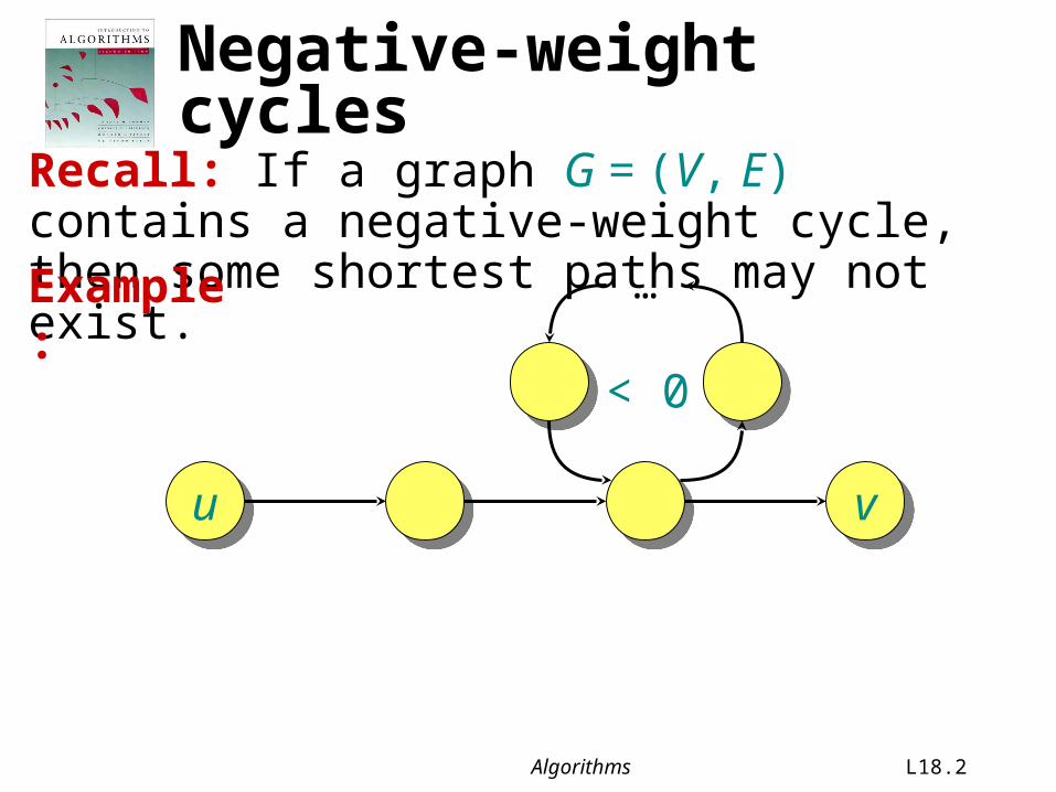
Negative-weight cyclesRecall: If a graph G = (V, E) contains a negative-weight cycle, then some shortest paths may not exist.Example:
u v
…
< 0
Algorithms L18.3
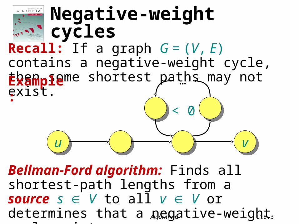
Negative-weight cyclesRecall: If a graph G = (V, E) contains a negative-weight cycle, then some shortest paths may not exist.Example:
u v
…
< 0
Bellman-Ford algorithm: Finds all shortest-path lengths from a source s V to all v V or determines that a negative-weight cycle exists.
Algorithms L18.4
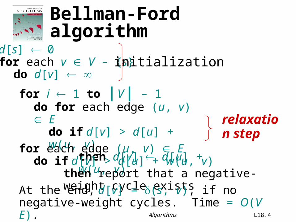
Bellman-Ford algorithmd[s] 0for each v V – {s}
do d[v]
for i 1 to | V | – 1do for each edge (u, v) E
do if d[v] > d[u] + w(u, v)then d[v] d[u] + w(u, v)
for each edge (u, v) Edo if d[v] > d[u] + w(u, v)
then report that a negative-weight cycle exists
initialization
At the end, d[v] = (s, v), if no negative-weight cycles. Time = O(V E).
relaxation step
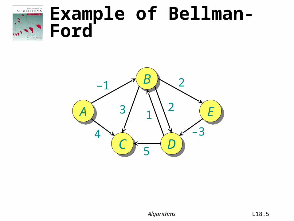
Algorithms L18.5
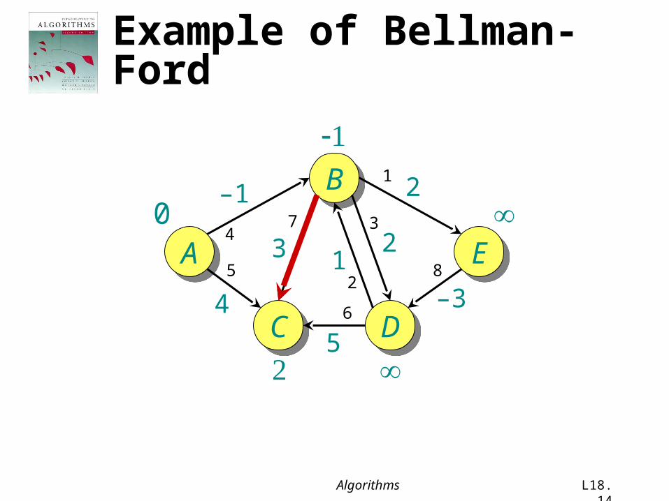
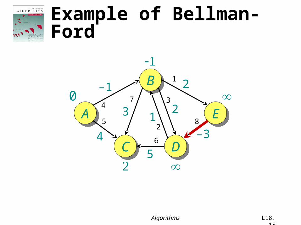
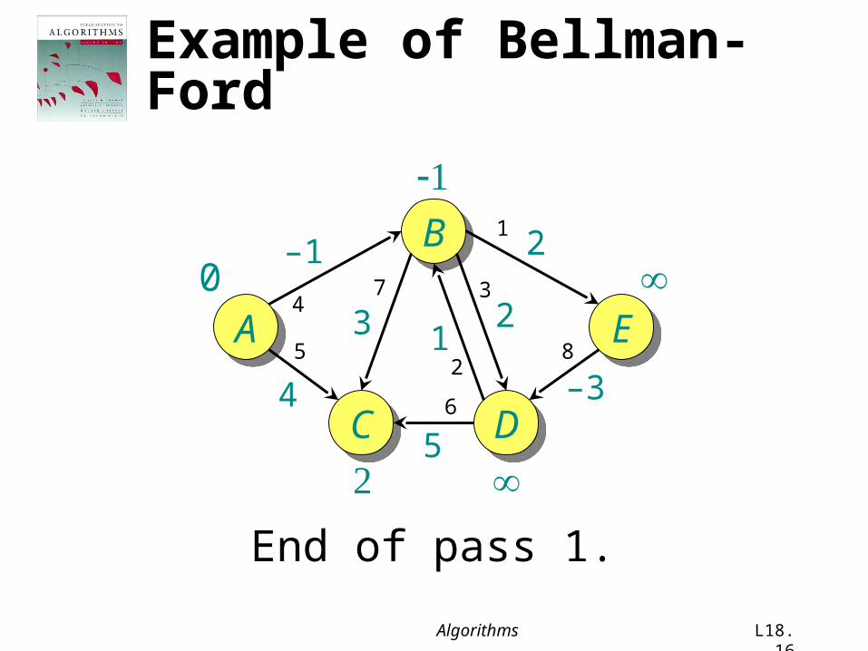
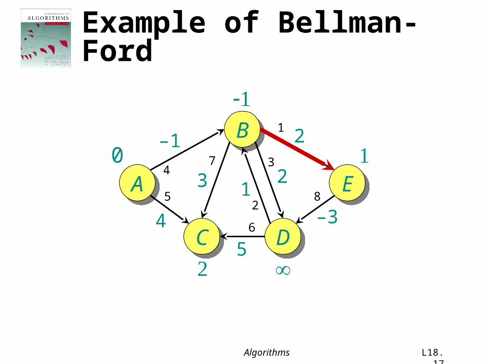
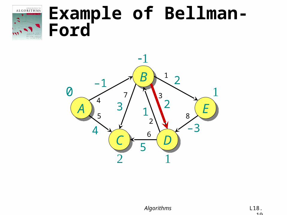
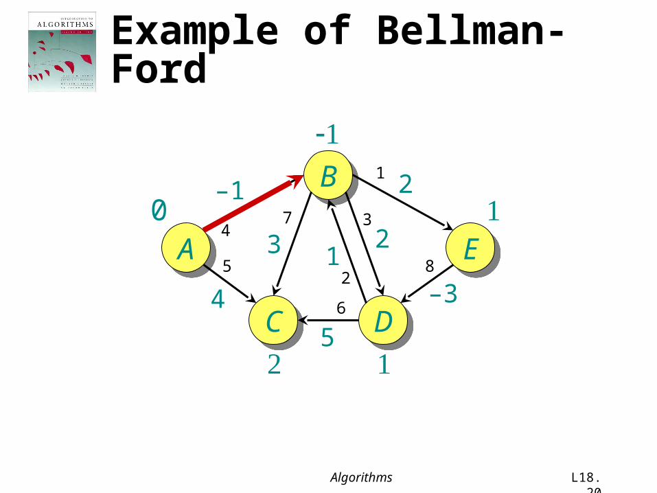
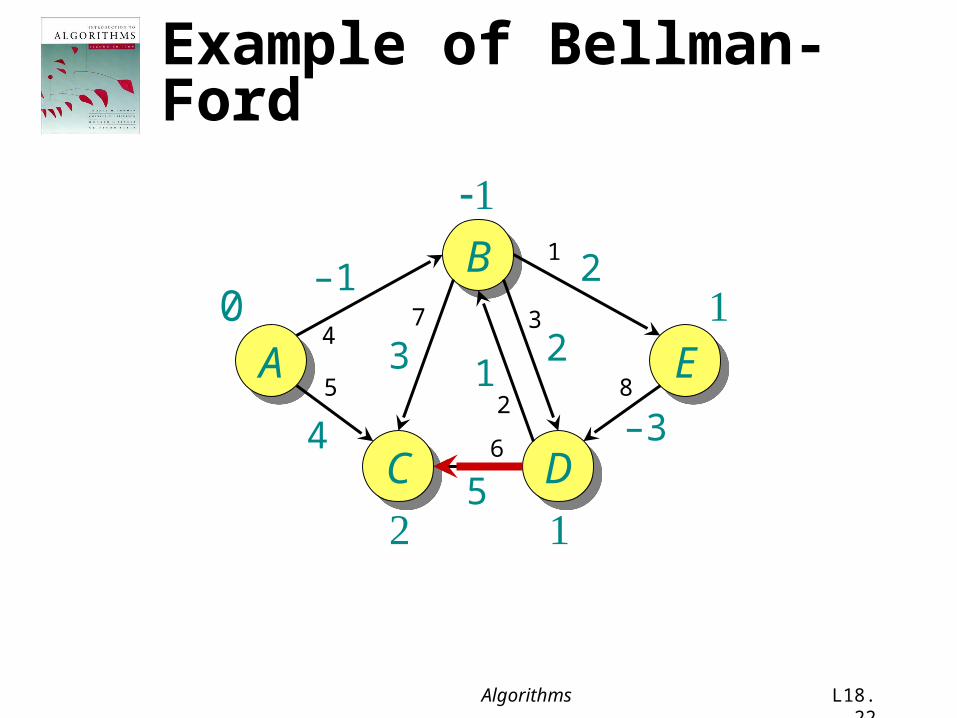
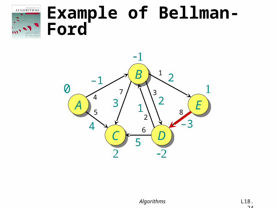
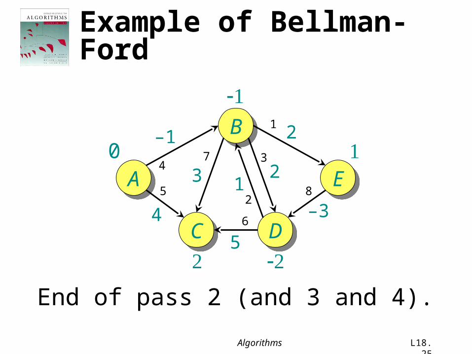
Example of Bellman-Ford
A
B
E
C D
–1
4
12
–3
2
5
3
Algorithms L18.6
Example of Bellman-Ford
A
B
E
C D
–1
4
12
–3
2
5
3
0
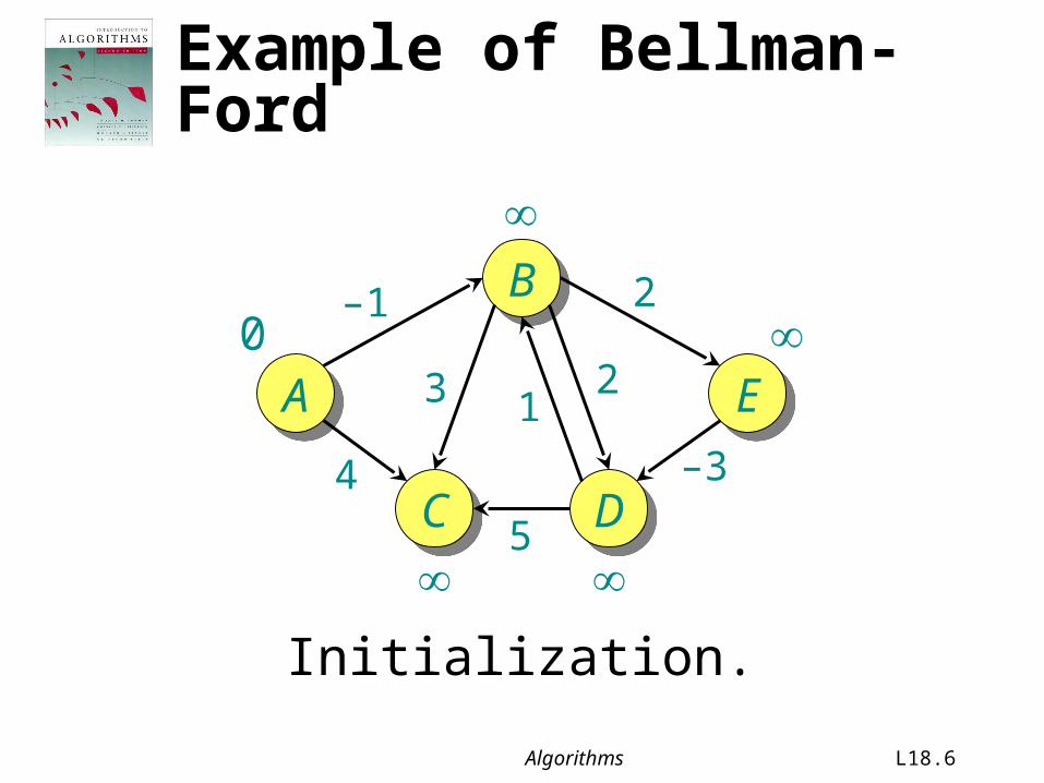
Initialization.
Algorithms L18.7
Example of Bellman-Ford
A
B
E
C D
–1
4
12
–3
2
5
3
0
1
2
34
5
7
8
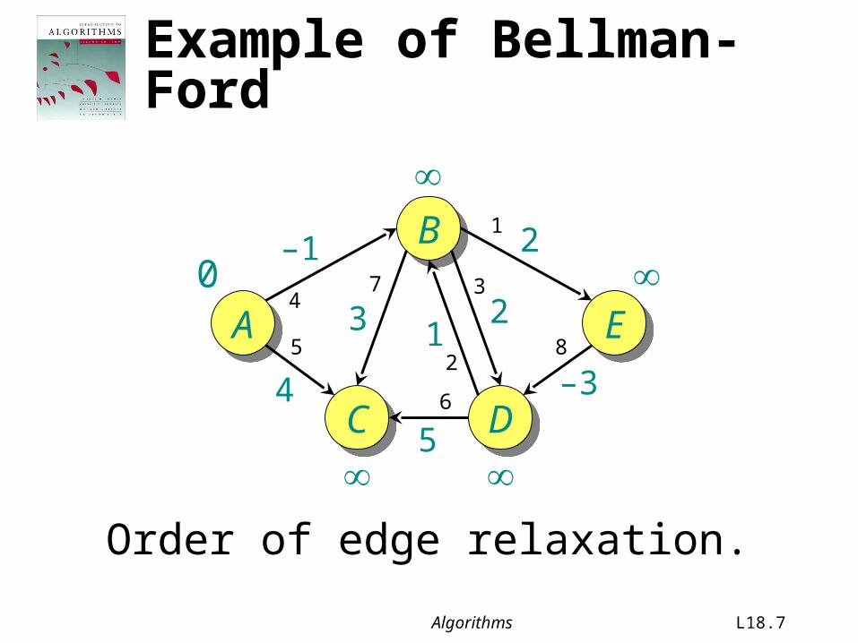
Order of edge relaxation.
6
Algorithms L18.8
Example of Bellman-Ford
A
B
E
C D
–1
4
12
–3
2
5
3
0
1
2
34
5
7
8
6
Algorithms L18.9
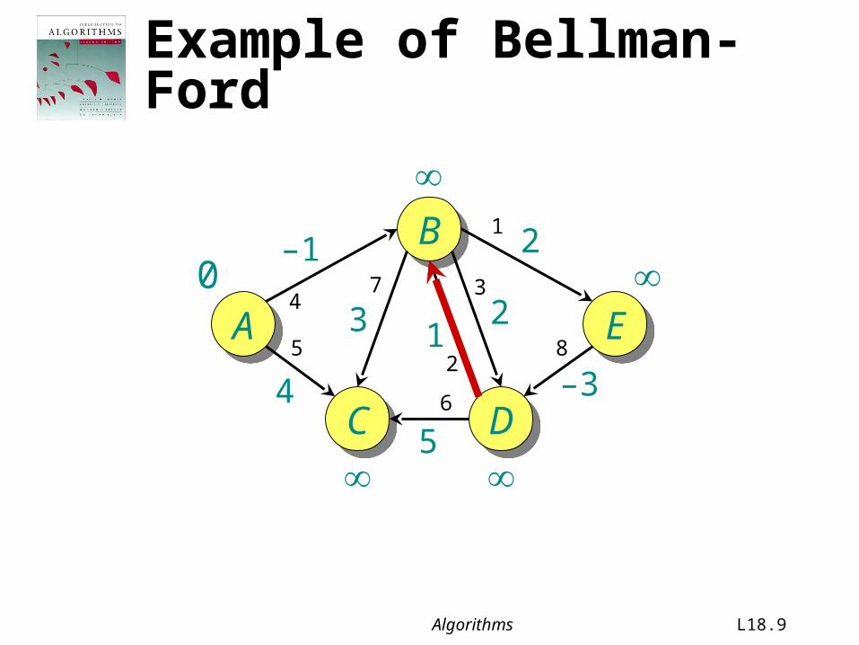
Example of Bellman-Ford
A
B
E
C D
–1
4
12
–3
2
5
3
0
1
2
34
5
7
8
6

Algorithms L18.10
Example of Bellman-Ford
A
B
E
C D
–1
4
12
–3
2
5
3
0
1
2
34
5
7
8
6
Algorithms L18.11
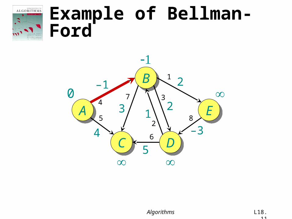
Example of Bellman-Ford
A
B
E
C D
–1
4
12
–3
2
5
30
1
2
34
5
7
8
6
Algorithms L18.12
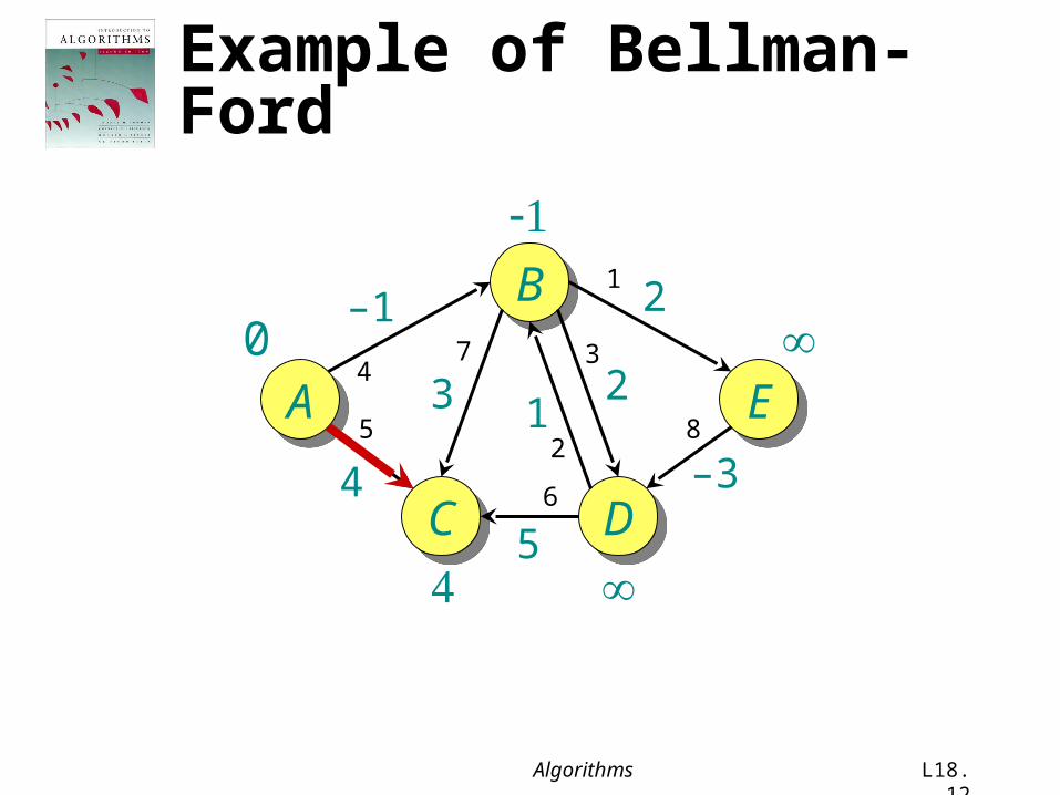
Example of Bellman-Ford
A
B
E
C D
–1
4
12
–3
2
5
30
1
2
34
5
7
8
6
Algorithms L18.13
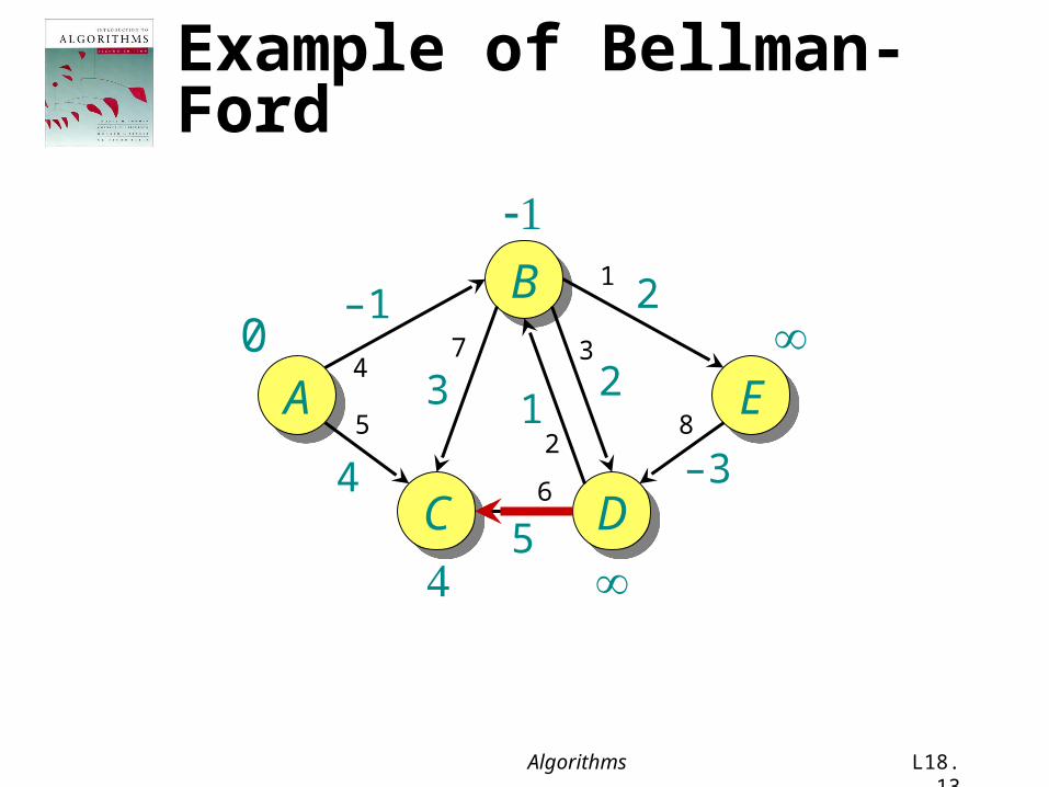
Example of Bellman-Ford
A
B
E
C D
–1
4
12
–3
2
5
30
1
2
34
5
7
8
6
Algorithms L18.14
Example of Bellman-Ford
A
B
E
C D
–1
4
12
–3
2
5
30
1
2
34
5
7
8
6
Algorithms L18.15
Example of Bellman-Ford
A
B
E
C D
–1
4
12
–3
2
5
30
1
2
34
5
7
8
6
Algorithms L18.16
Example of Bellman-Ford
A
B
E
C D
–1
4
12
–3
2
5
30
1
2
34
5
7
8
End of pass 1.
6
Algorithms L18.17
Example of Bellman-Ford
A
B
E
C D
–1
4
12
–3
2
5
30
1
2
34
5
7
8
6

Algorithms L18.18
Example of Bellman-Ford
A
B
E
C D
–1
4
12
–3
2
5
30
1
2
34
5
7
8
6
Algorithms L18.19
Example of Bellman-Ford
A
B
E
C D
–1
4
12
–3
2
5
30
1
2
34
5
7
8
6
Algorithms L18.20
Example of Bellman-Ford
A
B
E
C D
–1
4
12
–3
2
5
30
1
2
34
5
7
8
6

Algorithms L18.21
Example of Bellman-Ford
A
B
E
C D
–1
4
12
–3
2
5
30
1
2
34
5
7
8
6
Algorithms L18.22
Example of Bellman-Ford
A
B
E
C D
–1
4
12
–3
2
5
30
1
2
34
5
7
8
6

Algorithms L18.23
Example of Bellman-Ford
A
B
E
C D
–1
4
12
–3
2
5
30
1
2
34
5
7
8
6
Algorithms L18.24
Example of Bellman-Ford
A
B
E
C D
–1
4
12
–3
2
5
30
1
2
34
5
7
8
6
Algorithms L18.25
Example of Bellman-Ford
A
B
E
C D
–1
4
12
–3
2
5
30
1
2
34
5
7
8
6
End of pass 2 (and 3 and 4).
Algorithms L18.26
CorrectnessTheorem. If G = (V, E) contains no negative-weight cycles, then after the Bellman-Ford algorithm executes, d[v] = (s, v) for all v V.
Algorithms L18.27
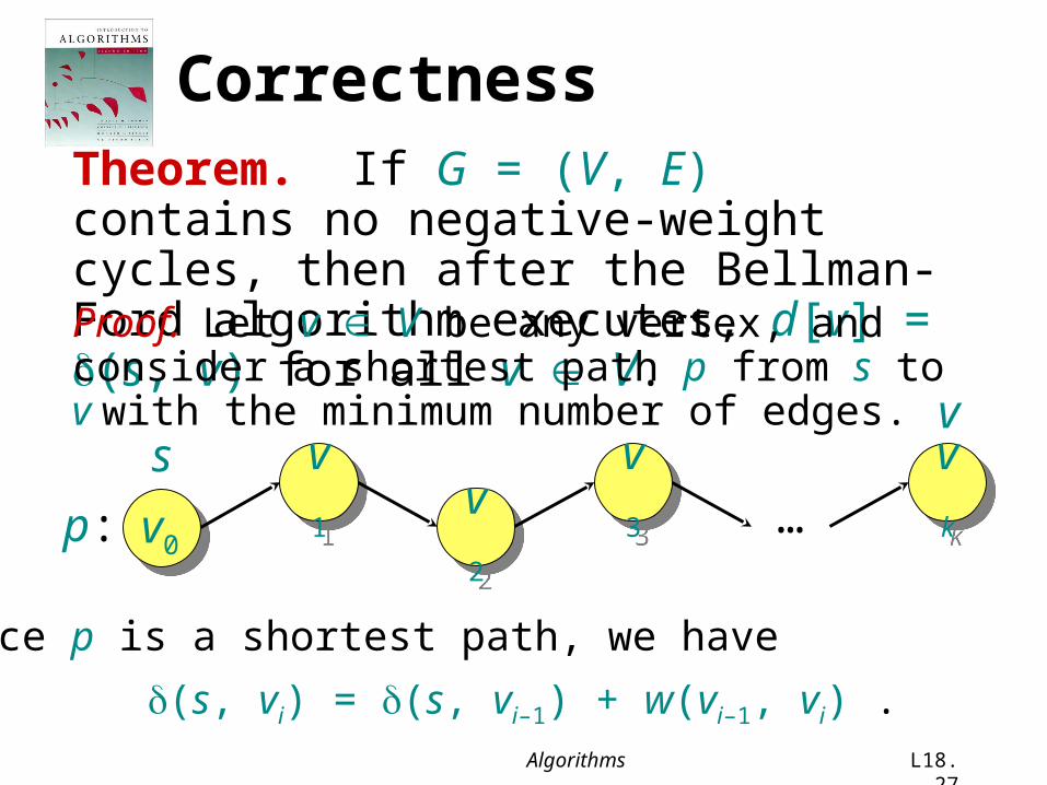
CorrectnessTheorem. If G = (V, E) contains no negative-weight cycles, then after the Bellman-Ford algorithm executes, d[v] = (s, v) for all v V. Proof. Let v V be any vertex, and consider a shortest path p from s to v with the minimum number of edges.
v1v2
v3 vkv0
…s
v
p:
Since p is a shortest path, we have(s, vi) = (s, vi–1) + w(vi–1, vi) .
Algorithms L18.28
Correctness (continued)
v1v2
v3 vkv0
…s
v
p:
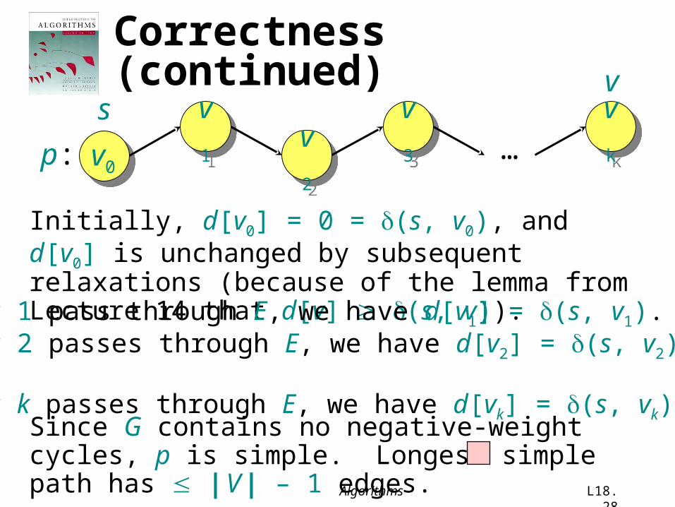
Initially, d[v0] = 0 = (s, v0), and d[v0] is unchanged by subsequent relaxations (because of the lemma from Lecture 14 that d[v] (s, v)).• After 1 pass through E, we have d[v1] = (s, v1).• After 2 passes through E, we have d[v2] = (s, v2).
• After k passes through E, we have d[vk] = (s, vk).Since G contains no negative-weight cycles, p is simple. Longest simple path has | V | – 1 edges.
Algorithms L18.29
Detection of negative-weight cycles
Corollary. If a value d[v] fails to converge after | V | – 1 passes, there exists a negative-weight cycle in G reachable from s.
Algorithms L18.30
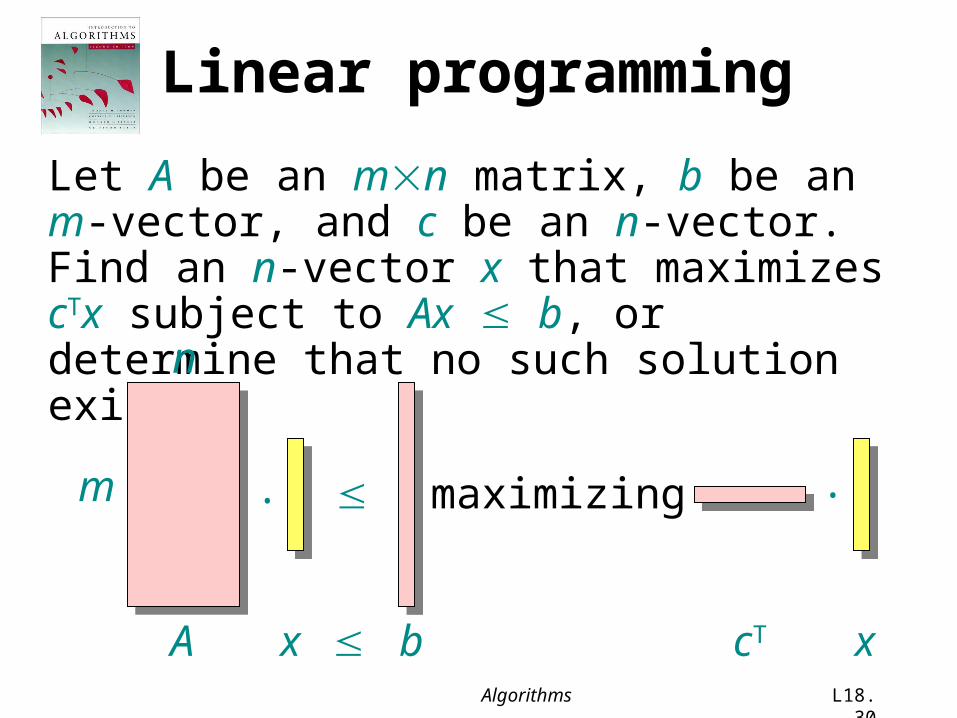
Linear programming
Let A be an mn matrix, b be an m-vector, and c be an n-vector. Find an n-vector x that maximizes cTx subject to Ax b, or determine that no such solution exists.
. .maximizingm
n
A x b cT x
Algorithms L18.31
Linear-programming algorithms
Algorithms for the general problem• Simplex methods — practical, but worst-case
exponential time.• Interior-point methods — polynomial time and
competes with simplex.
Algorithms L18.32
Linear-programming algorithms
Algorithms for the general problem• Simplex methods — practical, but worst-case
exponential time.• Interior-point methods — polynomial time and
competes with simplex.
Feasibility problem: No optimization criterion. Just find x such that Ax b.• In general, just as hard as ordinary LP.
Algorithms L18.33
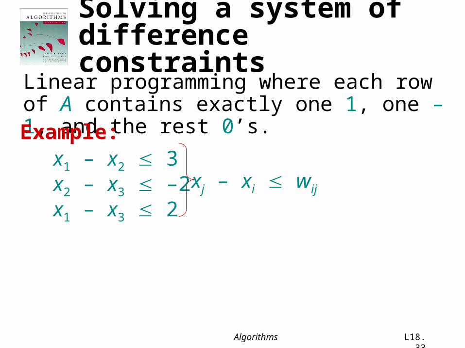
Solving a system of difference constraints
Linear programming where each row of A contains exactly one 1, one –1, and the rest 0’s. Example:
x1 – x2 3x2 – x3 –2x1 – x3 2
xj – xi wij
Algorithms L18.34
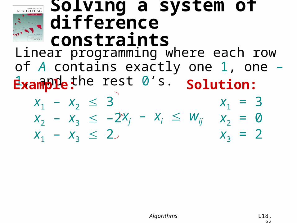
Solving a system of difference constraints
Linear programming where each row of A contains exactly one 1, one –1, and the rest 0’s. Example:
x1 – x2 3x2 – x3 –2x1 – x3 2
xj – xi wij
Solution:x1 = 3x2 = 0x3 = 2
Algorithms L18.35
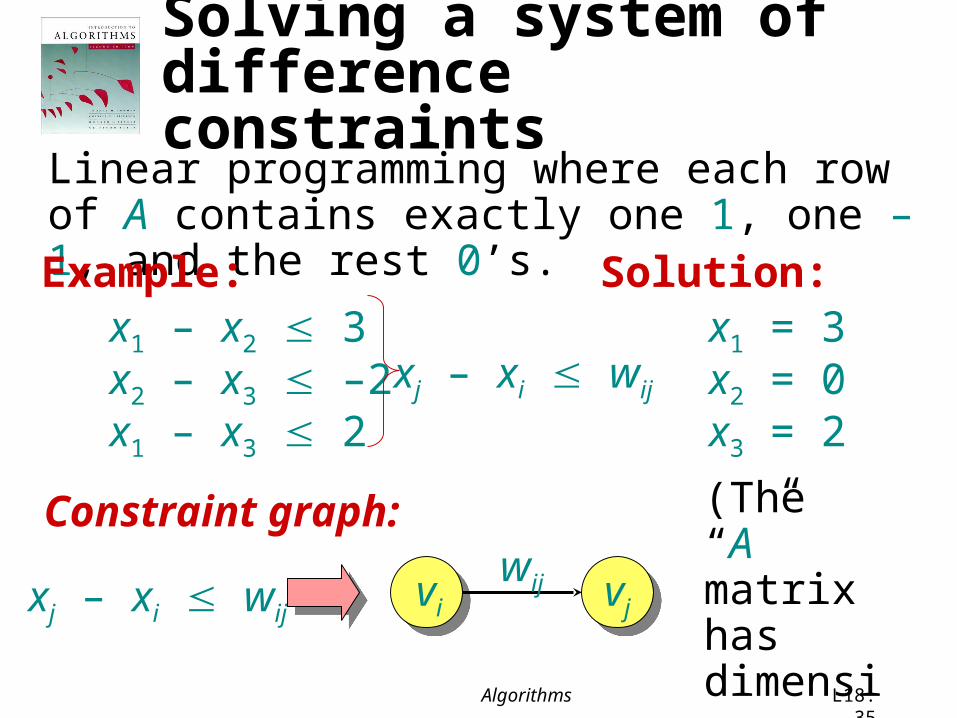
Solving a system of difference constraints
Linear programming where each row of A contains exactly one 1, one –1, and the rest 0’s. Example:
x1 – x2 3x2 – x3 –2x1 – x3 2
xj – xi wij
Solution:x1 = 3x2 = 0x3 = 2
Constraint graph:
vjvixj – xi wij
wij
(The “A” matrix has dimensions|E | |V |.)
Algorithms L18.36
Unsatisfiable constraintsTheorem. If the constraint graph contains a negative-weight cycle, then the system of differences is unsatisfiable.
Algorithms L18.37
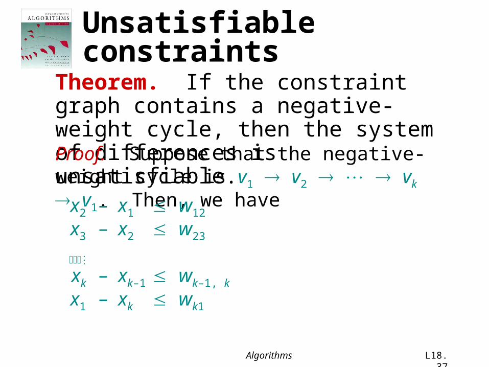
Unsatisfiable constraintsTheorem. If the constraint graph contains a negative-weight cycle, then the system of differences is unsatisfiable.Proof. Suppose that the negative-weight cycle is v1 v2 vk v1. Then, we have
x2 – x1 w12
x3 – x2 w23
xk – xk–1 wk–1, k
x1 – xk wk1
Algorithms L18.38
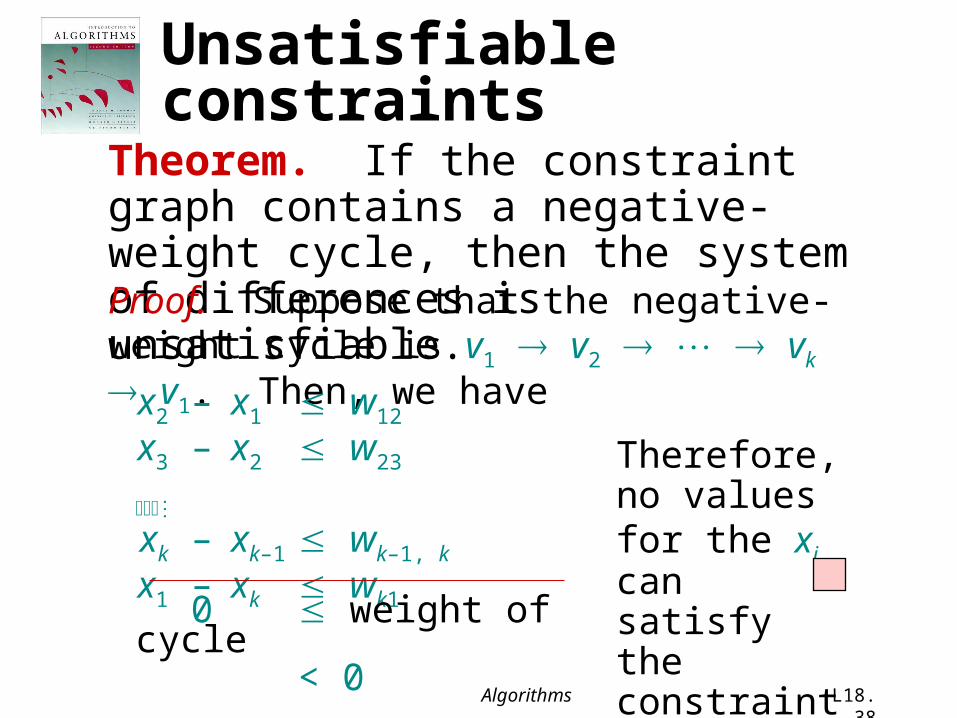
Unsatisfiable constraintsTheorem. If the constraint graph contains a negative-weight cycle, then the system of differences is unsatisfiable.Proof. Suppose that the negative-weight cycle is v1 v2 vk v1. Then, we have
x2 – x1 w12
x3 – x2 w23
xk – xk–1 wk–1, k
x1 – xk wk1
Therefore, no values for the xi can satisfy the constraints.
0 weight of cycle< 0
Algorithms L18.39
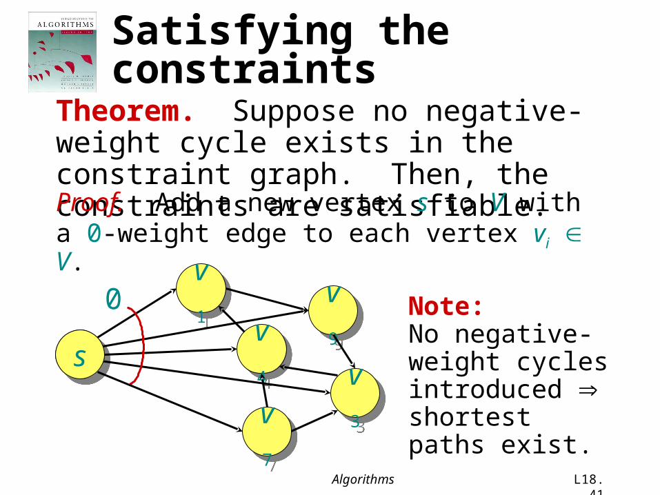
Satisfying the constraintsTheorem. Suppose no negative-weight cycle exists in the constraint graph. Then, the constraints are satisfiable.
Algorithms L18.40
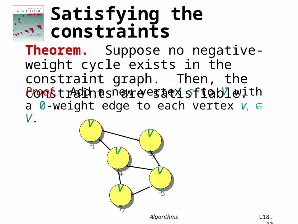
Satisfying the constraintsTheorem. Suppose no negative-weight cycle exists in the constraint graph. Then, the constraints are satisfiable.Proof. Add a new vertex s to V with a 0-weight edge to each vertex vi V.
v1
v4
v7
v9
v3
Algorithms L18.41
Satisfying the constraintsTheorem. Suppose no negative-weight cycle exists in the constraint graph. Then, the constraints are satisfiable.Proof. Add a new vertex s to V with a 0-weight edge to each vertex vi V.
v1
v4
v7
v9
v3
s
0 Note:No negative-weight cycles introduced shortest paths exist.

Algorithms L18.42
The triangle inequality gives us (s,vj) (s, vi) + wij. Since xi = (s, vi) and xj = (s, vj), the constraint xj – xi wij is satisfied.
Proof (continued)Claim: The assignment xi = (s, vi) solves the constraints.
s
vj
vi(s, vi)
(s, vj) wij
Consider any constraint xj – xi wij, and consider the shortest paths from s to vj and vi:

Algorithms L18.43
Bellman-Ford and linear programming
Corollary. The Bellman-Ford algorithm can solve a system of m difference constraints on n variables in O(m n) time. Single-source shortest paths is a simple LP problem.In fact, Bellman-Ford maximizes x1 + x2 + + xn subject to the constraints xj – xi wij and xi 0 (exercise).Bellman-Ford also minimizes maxi{xi} – mini{xi} (exercise).

Algorithms L18.44
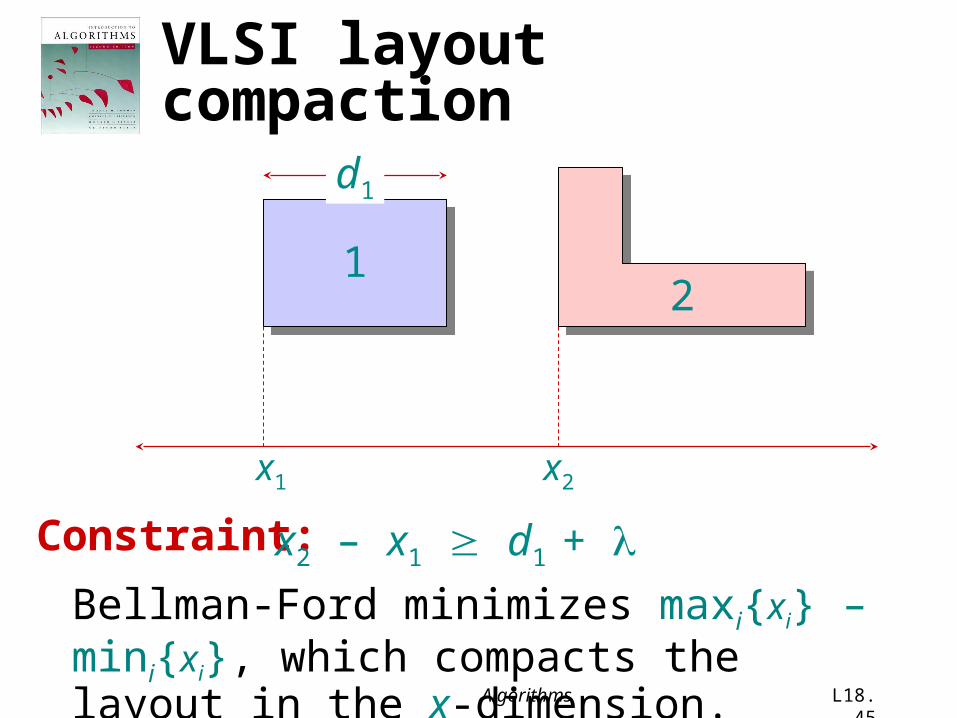
Application to VLSI layout compaction
Integrated-circuit features:
Problem: Compact (in one dimension) the space between the features of a VLSI layout without bringing any features too close together.
minimum separation
Algorithms L18.45
VLSI layout compaction
1
x1 x2
2
d1
Constraint: x2 – x1 d1 + Bellman-Ford minimizes maxi{xi} – mini{xi}, which compacts the layout in the x-dimension.