12 all pairs shortest paths

CS2010 – Data Structures and Algorithms II

Lecture 12 – Finding Your Wayfrom Any Point to Another Point (Part III)

[email protected]

OutlineOutline

• What are we going to learn in this lecture?– Quick Review: The Single‐Source Shortest Paths Problem

– Introducing: The All‐Pairs Shortest Paths Problem• With some motivating examples

– Floyd Warshall’s Dynamic Programming algorithm• The short code first

Th th DP f l ti (l )• Then the DP formulation (long one)

– Some Interesting Variants

The SSSP problem is aboutThe SSSP problem is about…

1. Finding the shortest path between a pair of vertices in the graph

2. Finding the shortest paths between any pair of vertices

3. Finding the shortest paths between one

0 00

pvertex to the other vertices in the graph

1 2 3

g p

0 of 120

What is the best SSSP algorithm on (+ or ‐) weighted general graph but without negative weight cycle?

1. DFS

2. BFS

3. Original Dijkstra’s

4 Modified Dijkstra’s4. Modified Dijkstra s

5. Bellman Ford’s

0 0 000

1 2 3 4 50 of 120

Let’s move on the next topic

ALL‐PAIRS SHORTEST PATHSLet s move on the next topic

What is your knowledge levelb t APSP ?about APSP now?

(each clicker can select up to 3 times)1. I have not heard about this

APSP problem or its solution beforesolution before

2. I know this problem and its four liner Floyd Warshall’sfour liner Floyd Warshall ssolution

3. I used it for PS4 :O

4. I used it for PS7 :O

5. I know how Floyd

0 0 000

5. I know how Floyd Warshall’s algorithm works, not just how to code that

1 2 3 4 50 of 120

four lines…

Motivating Problem 1gDiameter of a Graph

• The diameter of a graph is defined as the greatestshortest path distance between any pair of vertices

• For example, the diameter of this graph is 2– Paths with length equal to diameter are:

21

• 1‐0‐3 (or the reverse path)


0

2

3




4

0 3• 2‐3‐4 (or the reverse path)

4

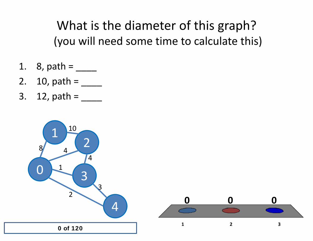
What is the diameter of this graph?(you will need some time to calculate this)

1. 8, path = ____

2. 10, path = ____

3. 12, path = ____

21

8 4

10

0 3

8 44

1

0 004

32

3

1 2 3

40 of 120

Motivating Problem 2gAnalyzing the average number of clicks to browse WWW

• In year 2000, only 19 clicks are necessary to move from any page on the WWW to any other page :O– That is, if the pages on the web are viewed as vertices in a graph, then the average path length between arbitrary

i f ti i th h i 19pairs of vertices in the graph is 19

– For example, the average path length between arbitrary pair of vertices in this graph below is:pair of vertices in this graph below is:

• 01 = 1; 02 = 1

• 10 = 2; 12 = 1 0 10 ;

• 20 = 1; 21 = 2• Average = (1+1+2+1+1+2) / 6 = 8 / 6 = 1.333

22

What is the average path length of this graph?(you will need some time to calculate this)

1. 22/10 = 2.200

2. 22/12 = 1.8332. 22/12 1.833

3. 23/12 = 1.917

0 1

0 0023

1 2 30 of 120

Motivating Problem 3gFinding the best meeting point

• Given a weighted graph that model a city and the travelling time between various places in that city– Find the best meeting point for two persons (there are lots of such queries), one is currently in A and the other is in B

– For example, the best meeting point between two persons currently in A = 0 and B = 3 is at vertex 2

B j t d 1 it f ti t lk f 32 d th it f A• B just need 1 unit of time to walk from 32 and then wait for A

• A needs 12 units of time to walk from 02

• After 12 units of time, they meet AAfter units of time, they meet

0 110

27 25

A

23418

B

What is the best meeting point for C and D?(you will need some time to calculate this)

1. Vertex 0, ___ units of time




10 D


0 110

27 25

D

0 0 000

23418

C

1 2 3 4 50 of 120

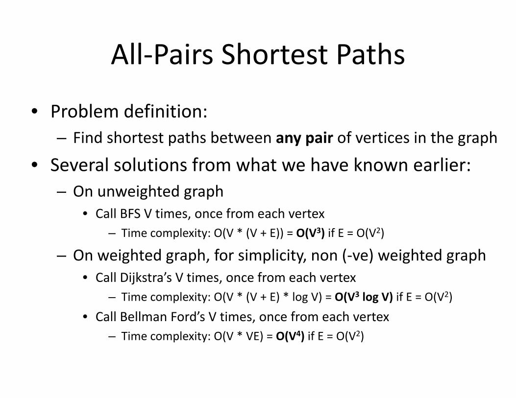
All Pairs Shortest PathsAll‐Pairs Shortest Paths

• Problem definition:– Find shortest paths between any pair of vertices in the graph

• Several solutions from what we have known earlier:– On unweighted graphg g p

• Call BFS V times, once from each vertex– Time complexity: O(V * (V + E)) = O(V3) if E = O(V2)

– On weighted graph, for simplicity, non (‐ve) weighted graph• Call Dijkstra’s V times, once from each vertex

Time complexity: O(V * (V + E) * log V) = O(V3 log V) if E = O(V2)– Time complexity: O(V * (V + E) * log V) = O(V3 log V) if E = O(V2)

• Call Bellman Ford’s V times, once from each vertex– Time complexity: O(V * VE) = O(V4) if E = O(V2)

Floyd Warshall’s Sneak PreviewFloyd Warshall s – Sneak Preview

W Adj M i• We use an Adjacency Matrix: D[|V|][|V|]– Originally D[i][j] contains the weight of edge(i, j) O(1)Af Fl d W h ll’ i i h i h f h(i j)– After Floyd Warshall’s stop, it contains the weight of path(i, j)

– It is usually a nice algorithm for the pre‐processing part

for (int k = 0; k < V; k++) // remember, k firstfor (int i = 0; i < V; i++) // before ifor (int j = 0; j < V; j++) // then jfor (int j = 0; j < V; j++) // then jD[i][j] = Math.min(D[i][j], D[i][k] + D[k][j]);

O(V3) i h th t d l !• O(V3) since we have three nested loops!– Apparently, if we only given a short amount of time, we can only solve the APSP problem for small graph as none of theonly solve the APSP problem for small graph, as none of the APSP solution shown here runs better than O(V3)…

Preprocessing + (Lots of) QueriesPreprocessing + (Lots of) Queries

• This is another problem solving technique

• Preprocess the data once (can be a costly operation)

• But then future queries can be (much) fasterby working on the processed databy working on the processed data

• Example with APSP problem:Once we have pre processed the APSP information with– Once we have pre‐processed the APSP information with O(V3) Floyd Warshall’s algorithm…

– Future queries that asks “what is the shortest path weightFuture queries that asks what is the shortest path weight between vertex i and j” can now be answered in O(1)…

Floyd Warshall’s Basic Idea (1)Floyd Warshall s – Basic Idea (1)

• Assume that the vertices are labeled as [0 .. V ‐ 1].

• Now let sp(i, j, k) denotes the shortest path between vertex i and t j ith th t i ti th t th ti th h t t thvertex j with the restriction that the vertices on the shortest path

(excluding i and j) can only consist of vertices from [0 .. k]– How Robert Floyd and Stephen Warshall managed to arrive at thisHow Robert Floyd and Stephen Warshall managed to arrive at this

formulation is beyond this lecture…

• Initially k = ‐1 (or to say, we only use direct edges only)– Then, iteratively add k by one until k = V ‐ 1

kkj

i


12 4

Suppose we want to know the shortest path between vertex 3

0 3

3

1

1 shortest path between vertex 3 and 4, using any intermediate vertices from k = [0 .. 4], i.e.

1 533

sp(3, 4, 4)

( ) ?

2 41

sp(3, 4, 4) = ?


i = 3 j = 4 k = ‐11

2 4

k 1 0 1 2 3 4

The current content of Adjacency Matrix D at k = ‐1

i = 3, j = 4, k = 1Direct Edges Only

0 3

3

1

1

k = ‐1 0 1 2 3 4

0 0 2 1 3

1 0 4

1 533

1 0 4

2 1 0 1

3 1 3 0 52 4

1

(3 4 1) 5( ) 3 ( ) 1

3 1 3 0 5

4 0

sp(3, 4, ‐1) = 5sp(3, 2, ‐1) = 3 sp(2, 4, ‐1) = 1

We will monitor these two values


i = 3 j = 4 k = 01

2 4Vertex 0 allowed

k 0 0 1 2 3 4

The current content of Adjacency Matrix D at k = 0

i = 3, j = 4, k = 0

0 3

3

1

1

k = 0 0 1 2 3 4

0 0 2 1 3

1 0 4

1 53

31 0 4

2 1 0 1

3 1 3 2 0 42 4

1

( ) 4( ) 2 ( ) 1

3 1 3 2 0 4

4 0

sp(3, 4, 0) = 4sp(3, 2, 0) = 2 sp(2, 4, 0) = 1


i = 3 j = 4 k = 11

2 4

k 1 0 1 2 3 4


i = 3, j = 4, k = 1Vertex 0‐1 allowed

0 3

3

1

1

k = 1 0 1 2 3 4

0 0 2 1 6 3

1 0 4

1 533

1 0 4

2 1 0 5 1

3 1 3 2 0 42 4

1

(3 4 1) 4( ) 2 ( ) 1

3 1 3 2 0 4

4 0

sp(3, 4, 1) = 4sp(3, 2, 1) = 2 sp(2, 4, 1) = 1


i = 3 j = 4 k = 21

2 4

k 2 0 1 2 3 4



0 3

3

1

1

k = 2 0 1 2 3 4

0 0 2 1 6 2

1 0 4

1 53

31 0 4

2 1 0 5 1

3 1 3 2 0 32 4

1

( ) 3( ) 2 ( ) 1

3 1 3 2 0 3

4 0

sp(3, 4, 2) = 3sp(3, 2, 2) = 2 sp(2, 4, 2) = 1


i = 3 j = 4 k = 31

2 4

k 3 0 1 2 3 4



0 3

3

1

1

k = 3 0 1 2 3 4

0 0 2 1 6 2

1 5 0 6 4 7

1 53

31 5 0 6 4 7

2 6 1 0 5 1

3 1 3 2 0 32 4

1

( ) 3( ) 2 ( ) 1

3 1 3 2 0 3

4 0

sp(3, 4, 2) = 3sp(3, 2, 2) = 2 sp(2, 4, 2) = 1


i = 3 j = 4 k = 41

2 4

k 4 0 1 2 3 4



0 3

3

1

1

k = 4 0 1 2 3 4

0 0 2 1 6 2

1 5 0 6 4 7

1 53

31 5 0 6 4 7

2 6 1 0 5 1

3 1 3 2 0 32 4

1

( ) 3( ) 2 ( ) 1

3 1 3 2 0 3

4 0

sp(3, 4, 2) = 3sp(3, 2, 2) = 2 sp(2, 4, 2) = 1

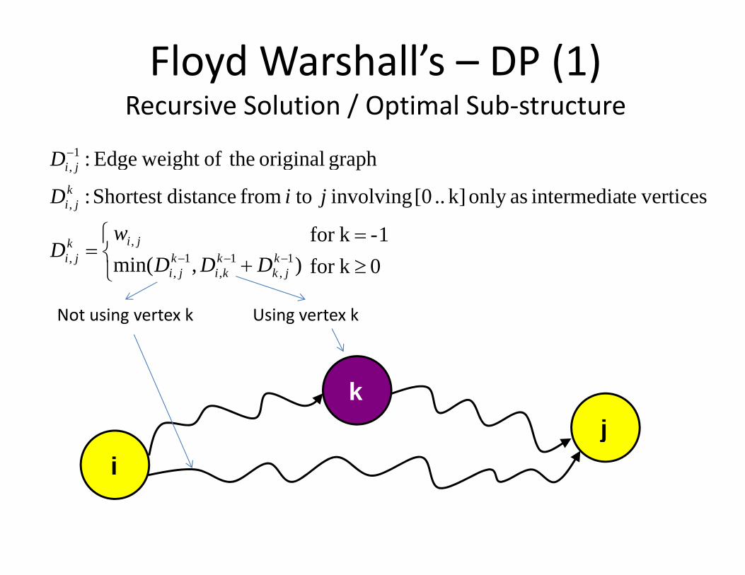
Floyd Warshall’s – DP (1)y ( )Recursive Solution / Optimal Sub‐structure

1

verticesteintermedia asonly k] .. [0 involving to from distanceShortest :

graphoriginal theof weight Edge:

,

1,

kji

ji

jiD

D

0 k for 1- k for

),min( 1,

1,

1,

,,

k

jkkki

kji

jikji DDD

wD

Not using vertex k Using vertex k

kj

ij

Floyd Warshall’s – DP (2)y ( )Overlapping Sub problems

• Avoiding re‐computation: To fill out an entry in the table k,we make use of entries in table k – 1, row by row, left to right

The topological order is obtained via 3 nested loops: k i j– The topological order is obtained via 3 nested loops: k i j

jk jjkk = 1 0 1 2 3 4

0 0 2 1 6 3

k = 2 0 1 2 3 4

0 0 2 1 6 2

j

k

0 0 2 1 6 3

1 0 4

2 1 0 5 1

0 0 2 1 6 2

1 0 4

2 1 0 5 1

ik 2 1 0 5 1

3 1 3 2 0 4

4 0

2 1 0 5 1

3 1 3 2 0 3

4 0

i

k=1 k=2

Floyd Warshall’s – DP (3)y ( )The Near Final Code

// th " f i dl " i O(V^3) l it// the "memory unfriendly" version, O(V^3) space complexityint[][][] D3 = new int[V+1][V][V]; // 3D matrixfor (k = 0; k <= V; k++) // initialization phasefor (i = 0; i < V; i++) { for (i 0; i V; i ) { Arrays.fill(D3[k][i], 1000000000); // cannot use nCopiesD3[k][i][i] = 0;

}

for (i = 0; i < E; i++) { // direct edgesu = sc.nextInt(); v = sc.nextInt(); w = sc.nextInt();D3[0][ ][ ] // di t d i ht d dD3[0][u][v] = w; // directed weighted edge

}

// main loop, O(V^3): this three nested loops are the "topological order"// p, ( ) p p gfor (k = 0; k < V; k++) // be careful, put k firstfor (i = 0; i < V; i++) // before ifor (j = 0; j < V; j++) // and then jD3[k+1][i][j] = Math.min(D3[k][i][j], // note, I shift index k by +1

D3[k][i][k] + D3[k][k][j]);

Floyd Warshall’s – DP (4)y ( )The Final Code, drop dimension ‘k’

i [][] i [ ][ ] // 2 dj iint[][] D = new int[V][V]; // 2D adjacency matrixfor (i = 0; i < V; i++) { // initialization phaseArrays.fill(D[i], 1000000000); // cannot use nCopiesD[i][i] = 0;

}for (i = 0; i < E; i++) { // direct edgesfor (i = 0; i < E; i++) { // direct edgesu = sc.nextInt(); v = sc.nextInt(); w = sc.nextInt();D[u][v] = w; // directed weighted edge

}// main loop, O(V^3): the "topological order"for (k = 0; k < V; k++) // be careful, put k firsto ( 0; ; ) // be ca e u , put stfor (i = 0; i < V; i++) // before ifor (j = 0; j < V; j++) // and then jD[i][j] M th i (D[i][j] D[i][k] D[k][j])D[i][j] = Math.min(D[i][j], D[i][k] + D[k][j]);

Floyd Warshall’s AlgorithmFloyd Warshall s Algorithm…

1. Code looks easy,but I still do not understand the DP formulationformulation

2. 50‐50

3. I understand both the code and the DP

0 00

the code and the DP formulation

1 2 30 of 120

5 minutes break, and then…

VARIANTS OF FLOYD WARSHALL’S5 minutes break, and then…

Variant 1 Print the Actual SP (1)Variant 1 – Print the Actual SP (1)

• We have learned to use array/Vector p (predecessor/ parent) to record the BFS/DFS/SP Spanning Tree– But now, we are dealing with all‐pairs of paths :O

• Solution: Use predecessor matrix p– let p be a 2D predecessor matrix, where p[i][j] is the last vertex before j on a shortest path from i to j, i.e. i ‐> ... ‐> p[i][j] ‐> j

– Initially, p[i][j] = i for all pairs of i and j

– If D[i][k] + D[k][j] < D[i][j], then D[i][j] = D[i][k] + D[k][j] and p[i][j] = p[k][j] this will be the last vertex before j in th h t t ththe shortest path

Variant 1 Print the Actual SP (2)Variant 1 – Print the Actual SP (2)D 0 1 2 3 4• The two matrices, D and p

– Shortest path from 3 ~ 4

D 0 1 2 3 4

0 0 2 1 6 3

1 5 0 6 4 7– 3024

1 5 0 6 4 7

2 6 1 0 5 1

3 1 3 2 0 31

2 4

3 1 3 2 0 3

4 0

0 3

3

1

1

p 0 1 2 3 4

0 0 0 0 1 2

1 53

3 1 3 1 0 1 2

2 3 2 2 1 2

3 3 0 0 3 22 41

3 3 0 0 3 2

4 4 4 4 4 4

Variant 2 Transitive Closure (1)Variant 2 – Transitive Closure (1)

• Stephen Warshall actually invented this algorithm for solving the transitive closure problem– Given a graph, determine if vertex i is connected to vertex jeither directly (via an edge) or indirectly (via a path)

• Solution: Modify the matrix D to contain only 0/1– In the main loop of Warshall’s algorithm:

// Initially: D[i][i] = 0// D[i][j] = 1 if edge(i j) exist; 0 otherwise// D[i][j] = 1 if edge(i, j) exist; 0 otherwise// the three nested loops as per normal

D[i][j] = D[i][j] | (D[i][k] & D[k][j]); // faster

Variant 2 Transitive Closure (2)Variant 2 – Transitive Closure (2)D,init 0 1 2 3 4• The matrix D,

before and after

D,init 0 1 2 3 4

0 0 1 1 0 1

1 0 0 0 1 0

2 0 1 0 0 1

3 1 0 1 0 11

2 4 4 0 0 0 0 0

0 3

3

1

1

D,final 0 1 2 3 4

0 1 1 1 1 1

1 1 1 1 1 11 5

33 1 1 1 1 1 1

2 1 1 1 1 1

3 1 1 1 1 12 4

1

3 1 1 1 1 1

4 0 0 0 0 0

Variant 3 Minimax/Maximin (1)Variant 3 – Minimax/Maximin (1)

• The minimax problem is a problem of finding the minimum of maximum edge weight along all possible paths from vertex i to vertex j (maximin is the reverse)– For a single path from i to j, we pick the maximum edgeweight along this path

– Then, for all possible paths from i to j, we pick the one with th i i d i htthe minimum max‐edge‐weight

• Solution: Again, a modification of Floyd Warshall’s// Initially: D[i][i] = 0// D[i][j] = weight of edge(i, j) exist; INF otherwise// the three nested loops as per normalp p

D[i][j] = Math.min(D[i][j], Math.max(D[i][k], D[k][j]));

Variant 3 Minimax/Maximin (2)Variant 3 – Minimax/Maximin (2)D,init 0 1 2 3 4• The minimax from 1 to 4

is 4, via edge (1, 3)

D,init 0 1 2 3 4

0 0 2 1 3

1 0 4 – 13024 2 1 0 1

3 1 3 0 51

2 4 4 0

0 3

3

1

1

D,final 0 1 2 3 4

0 0 1 1 4 1

1 4 0 4 4 41 5

33 1 4 0 4 4 4

2 4 1 0 4 1

3 1 1 1 0 12 4

1

3 1 1 1 0 1

4 0

Variant 4 Safest Paths (1)Variant 4 – Safest Paths (1)

• Given a directed graph where the edge weights represent the survival probabilities of passing through that edge, your task is to compute the safest path between two vertices– i.e. the path that maximizes the product of probabilitiesalong the path

• Solution: again, modification of Floyd Warshall’s// Initially, D[i][i] = 1.0// [i][j] i h (i j) 0 0 h i// D[i][j] = weight(i, j), 0.0 otherwise// the three nested loops as per normal

D[i][j] = Math.max(D[i][j], D[i][k] * D[k][j]);[ ][j] ( [ ][j], [ ][ ] [ ][j]);

Variant 4 Safest Paths (2)Variant 4 – Safest Paths (2)D,init 0 1 2 3 4• The safest path from 1 to 4

is 0.20, via this path

D,init 0 1 2 3 4

0 1.00 0.20 0.10 0.00 0.30

1 0.00 1.00 0.00 0.40 0.00– 134 2 0.00 0.10 1.00 0.00 0.10

3 0.10 0.00 0.30 1.00 0.501

0.2 0.4 4 0.00 0.00 0.00 0.00 1.00

0 3

0 3

0.1

0.1

D,final 0 1 2 3 4

0 1.00 0.20 0.10 0.08 0.30

1 0 04 1 00 0 12 0 40 0 200.1 0.5

0.30.3 1 0.04 1.00 0.12 0.40 0.20

2 0.00 0.10 1.00 0.04 0.10

3 0 10 0 03 0 30 1 00 0 502 4

0.1

3 0.10 0.03 0.30 1.00 0.50

4 0.00 0.00 0.00 0.00 1.00

Java ImplementationsJava Implementations

• Let’s see: FloydWarshallDemo.java

• Let’s see how easy to change the basic form ofFloyd Warshall’s algorithm to its variants

• Note: That Java file is not written in OOP fashion…Note: That Java file is not written in OOP fashion…– Please re‐factor it if you need to use it for other projects!

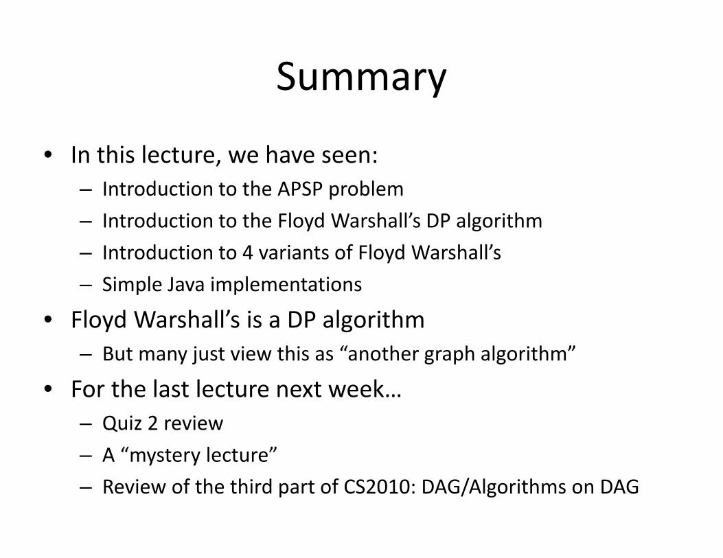
SummarySummary

• In this lecture, we have seen:– Introduction to the APSP problem

– Introduction to the Floyd Warshall’s DP algorithm

– Introduction to 4 variants of Floyd Warshall’s

Si l J i l t ti– Simple Java implementations

• Floyd Warshall’s is a DP algorithmB j i hi “ h h l i h ”– But many just view this as “another graph algorithm”

• For the last lecture next week…– Quiz 2 review

– A “mystery lecture”

R i f th thi d t f CS2010 DAG/Al ith DAG– Review of the third part of CS2010: DAG/Algorithms on DAG

12 all pairs shortest paths

Documents