10.25.2012 - craig mcintosh
DESCRIPTION
Slum Infrastructure Upgrading and Budget Spillovers: The Case of Mexico's Habitat ProgramTRANSCRIPT

Slum Infrastructure Upgrading & Budgeting Spillovers: The Case of Mexico’s Hábitat Program
IFPRI, Washington DC, Oct. 25, 2012.
Tito Alegria, El COLEF Craig McIntosh, UCSD
Gerardo Ordoñez, El COLEF Rene Zenteno, El COLEF

Policy Experiments at the Micro and Macro level
Explosion of development research on micro-interventions: • Cash transfers (Skoufias & Parker 2001, Fiszbein et al. 2009) • Health: deworming (Miguel & Kremer 2003), bednets (Dupas 2009,
Tarozzi et al. 2011) Research-driven agenda will under-invest in macro-level interventions that are hard to evaluate? • We know that infrastructure is critical for the welfare of the urban poor,
but how to quantify these effects? Most extant studies on infrastructure are observational: • staggered rollout (Dercon et al. 2006, Galiani et al. 2008, Galiani &
Shargrodsky 2010) • matching (Chase 2002, Newman et al. 2002) • instrumental variables (Paxson & Schady 2002, Duflo & Pande 2007).
2

Need to push good research design towards macro-level policies
This paper part of a very new literature providing experiments in infrastructure (Newman et al. 1994):
• Gonzales-Navarro & Quintana-Domeque 2011 examine a street-paving experiment in one town: Acayucan (Veracruz), Mexico
• Kremer et al. 2011 randomize placement of water infrastructure across 186 springs in Kenya
This study is unique in that it: 1. Is huge in absolute scale ($65 million in investment moved through the
experiment.) 2. Covers most of urban Mexico (20 states, 60 municipalities) 3. Accompanied by detailed household & block-level data collection
(9,702 household surveys in a two-period panel) 4. Is an evaluation ‘at scale’ of a major program administered by the federal
government 5. Features a ‘Randomized Saturation’ design to understand the interplay
between infrastructure investment at the federal and local levels.
3

What is Programa Hábitat? • Hábitat, designed by SEDESOL, through the Care Programme Unit of Urban
Poverty (UPAPU), aims to "contribute to overcoming poverty and improving the quality of life of people in marginalized urban areas, strengthening and improving the organization and social participation and the urban environment of those settlements" (Rules of Operation, Hábitat 2009).
• Hábitat invests only in neighborhoods that are:
– ‘marginalized’ neighborhoods in cities w > 15,000 residents. – without active conflicts over land tenure, . Home ownership rates in these
neighborhoods very high (84%) and most own houses outright (74% of total sample). This turns out to be important!
• Unique dimension of Habitat intervention is focus on community
development, not just infrastructure. Social capital outcomes are a central concern in this evaluation for SEDESOL & the IDB.
4

Where did the Hábitat experiment take place?
5
Control Tratamiento Total Baja California 6 14 20 Campeche 3 1 4 Chiapas 2 1 3 Chihuahua 6 5 11 Coahuila 3 3 6 Distrito Federal 16 20 36 Guanajuato 7 13 20 Guerrero 9 7 16 Jalisco 14 10 24 México 46 40 86 Michoacán 6 13 19 Morelos 4 3 7 Nuevo León 4 3 7 Puebla 24 15 39 Quintana Roo 12 1 13 Sinaloa 6 7 13 Sonora 6 1 7 Tamaulipas 8 12 20 Veracruz 9 5 14 Yucatán 3 2 5 Total 194 176 370
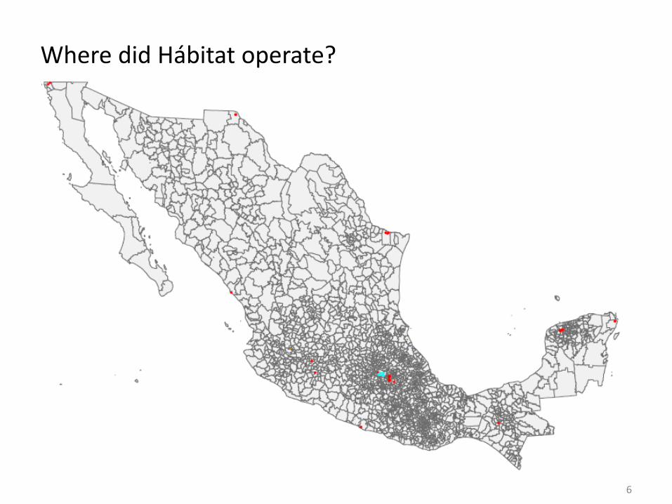
Where did Hábitat operate?
6
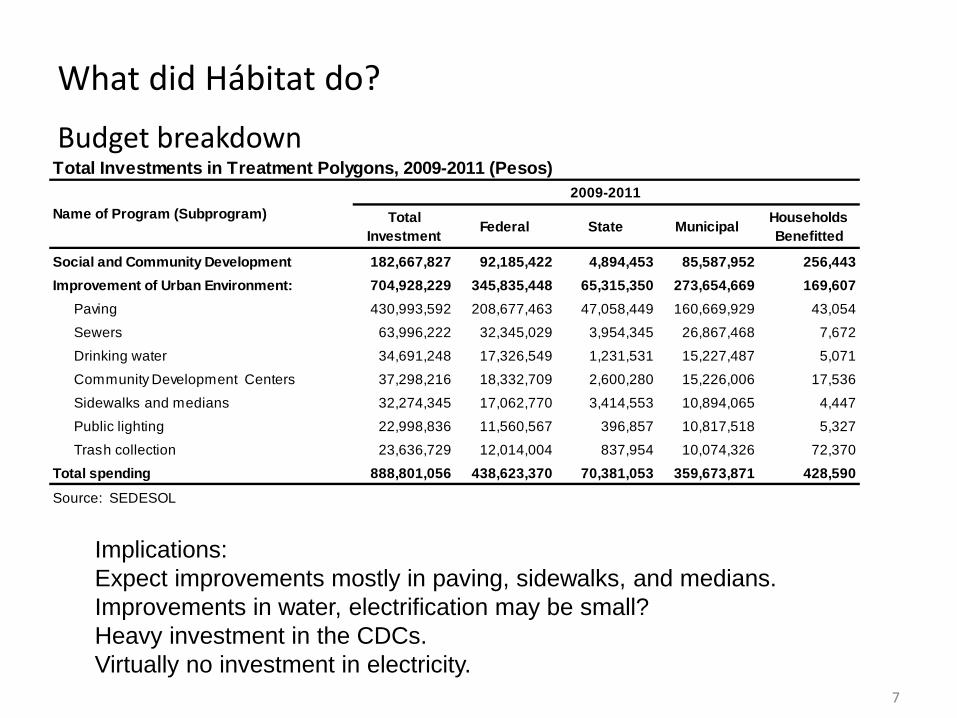
What did Hábitat do? Budget breakdown
7
Implications: Expect improvements mostly in paving, sidewalks, and medians. Improvements in water, electrification may be small? Heavy investment in the CDCs. Virtually no investment in electricity.
Total Investments in Treatment Polygons, 2009-2011 (Pesos)
Total Investment Federal State Municipal Households
Benefitted
Social and Community Development 182,667,827 92,185,422 4,894,453 85,587,952 256,443Improvement of Urban Environment: 704,928,229 345,835,448 65,315,350 273,654,669 169,607
Paving 430,993,592 208,677,463 47,058,449 160,669,929 43,054
Sewers 63,996,222 32,345,029 3,954,345 26,867,468 7,672
Drinking water 34,691,248 17,326,549 1,231,531 15,227,487 5,071
Community Development Centers 37,298,216 18,332,709 2,600,280 15,226,006 17,536
Sidewalks and medians 32,274,345 17,062,770 3,414,553 10,894,065 4,447
Public lighting 22,998,836 11,560,567 396,857 10,817,518 5,327
Trash collection 23,636,729 12,014,004 837,954 10,074,326 72,370
Total spending 888,801,056 438,623,370 70,381,053 359,673,871 428,590
Source: SEDESOL
Name of Program (Subprogram)2009-2011

Two core research design challenges in this study:
1. Federal and municipal governments are both responsible for building infrastructure. – Well-informed local agent (municipal government) will re-optimize
around the research design? – Local governments also required to match federal spending. – Spillovers & implications for causal inference even with an RCT?
2. Unit of randomization is the ‘polygon’ (slum or colonia), unit of intervention is smaller (street paved, community center built), and unit of analysis is smaller still (household). – How to analyze Treatment on Treated? – Need to collect large number of household surveys to have
households close to interventions, even though ‘design effect’ suggests that this won’t add much power to the ITT (intracluster correlations of infrastructure variables are as high as .55).
8

The multi-level budgeting game
Consider the problem of a national-level and local-level politician allocating spending and , respectively, to locality i.
• Make the extreme assumption that voters have no ability to attribute spending to the correct entity, and politicians thus face re-election probabilities and , with and .
• The local-level politician takes as given and maximizes subject to a budget constraint, where 𝜎𝑖 is the locality-level vote share. FOC:
9
iS is
( )i i iP S s+ ( )i i ip S s+
, 0i iP p′ ′ > , 0i iP p′′ ′′ <
iS
( )i i ii
p S s+∑
i jp p i j′ ′= ∀ ≠

The rules of matched federal spending:
Then, the national-level politician enters into an experiment that exogenously increases for a randomly selected subset of treatment localities for which , also requires that local government matches spending .
Former effect makes municipalities want to push funding from treated to control locations, but matching requirement forces them to spend in the treatment group.
Now: s.t. So, what will happen in equilibrium and what is the effect on
causal inference in this RCT? Three cases; analogy to ‘infra-marginality’ in the literature on
food aid (Moffit 1989, Gentili 2007).
10
iS
i ik mK=1iT =
( )max i
i i i i is ip S K s k+ + +∑ ( )i i
is k B+ ≤∑

Impacts on municipal spending: three groups.
1. Infra-marginal: Municipal governments were spending more on treatment locations prior to experiment than the match amount plus the residual that they want to leave in after redistributing the federal infrastructure spending optimally. No difference between treatment and control in equilibrium, so even if . Complete crowdout, maximal spillovers, no treatment effects.
11
( )*0i i i is k K Kστ> + −
( )( ) ( )( )* *| 1 | 0i i i i i i i iITT E f S K s k T E f S s T≡ + + + = − + =( ) 0df K
dK ≠
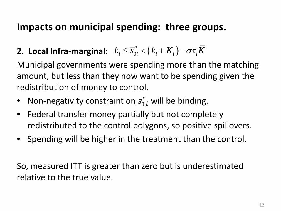
Impacts on municipal spending: three groups.
2. Local Infra-marginal: Municipal governments were spending more than the matching amount, but less than they now want to be spending given the redistribution of money to control. • Non-negativity constraint on 𝑠1𝑖∗ will be binding. • Federal transfer money partially but not completely
redistributed to the control polygons, so positive spillovers. • Spending will be higher in the treatment than the control. So, measured ITT is greater than zero but is underestimated relative to the true value.
12
( )*0i i i i ik s k K Kστ≤ < + −
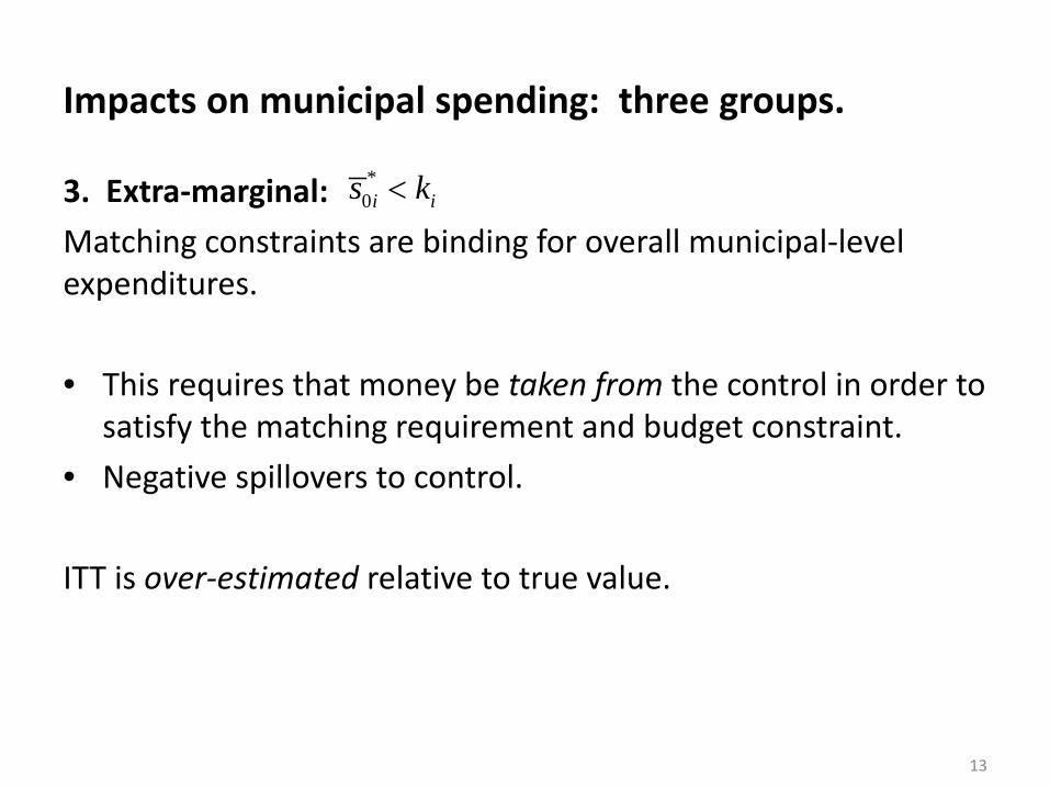
Impacts on municipal spending: three groups.
3. Extra-marginal: Matching constraints are binding for overall municipal-level expenditures. • This requires that money be taken from the control in order to
satisfy the matching requirement and budget constraint. • Negative spillovers to control. ITT is over-estimated relative to true value.
13
*0i is k<

Usefulness of the Randomized Saturation design:
• The experiment operates within a large number (60) of local-level governments, each of which provides over an average of 5.7 Hábitat-defined polygons (colonias).
• Two-level research design: 1. First assign each municipality a ‘saturation’ (drawn from a uniform
distribution between .1 and .9) that is the fraction of polygons to be treated.
2. Then, conditional on this municipal-level saturation, assign treatment randomly at the polygon level.
• This provides experimental variation in spillover effects on both the treatment and the control (Crepon et al., 2011, Baird et al. 2012).
14
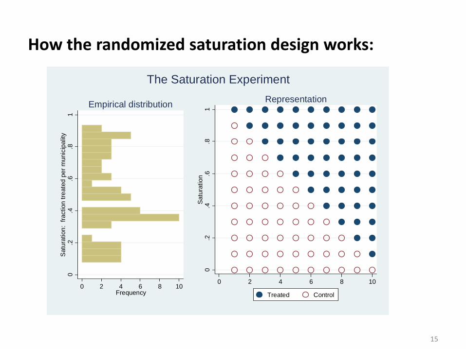
How the randomized saturation design works:
15
0
.2.4
.6.8
1S
atur
atio
n: f
ract
ion
treat
ed p
er m
unic
ipal
ity
0 2 4 6 8 10Frequency
Empirical distribution
0.2
.4.6
.81
Sat
urat
ion
0 2 4 6 8 10
Treated Control
Representation
The Saturation Experiment
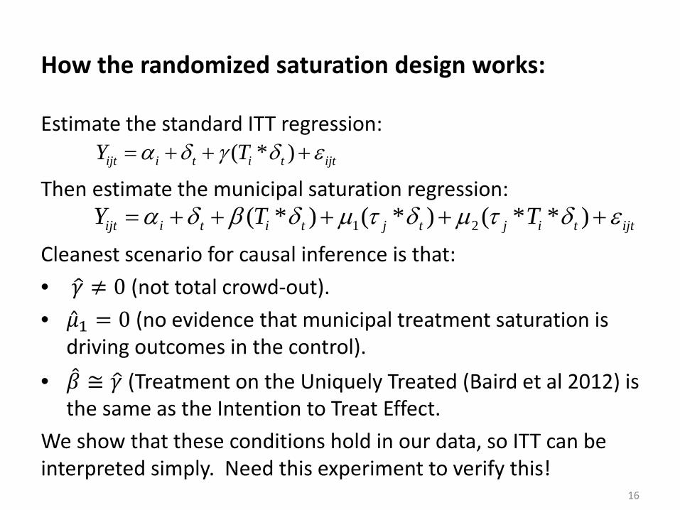
How the randomized saturation design works:
16
Estimate the standard ITT regression: Then estimate the municipal saturation regression: Cleanest scenario for causal inference is that: • 𝛾� ≠ 0 (not total crowd-out). • �̂�1 = 0 (no evidence that municipal treatment saturation is
driving outcomes in the control). • �̂� ≅ 𝛾� (Treatment on the Uniquely Treated (Baird et al 2012) is
the same as the Intention to Treat Effect. We show that these conditions hold in our data, so ITT can be interpreted simply. Need this experiment to verify this!
( * )ijt i t i t ijtY Tα δ γ δ ε= + + +
1 2( * ) ( * ) ( * * )ijt i t i t j t j i t ijtY T Tα δ β δ µ τ δ µ τ δ ε= + + + + +
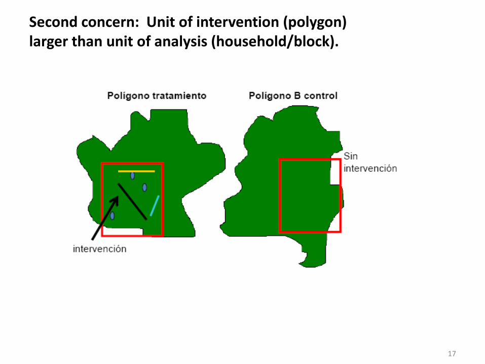
Second concern: Unit of intervention (polygon) larger than unit of analysis (household/block).
17

18
Why we survey so many blocks:
The rationale of including a large number of blocks is the desire to push the study down to the block level, instead of the polygon. Why? Arguments against this are:
• The randomization was not done at block level, so you have to use non-experimental techniques to do so.
• It creates little extra power at the polygon level due to clustering, and is expensive.
The problem is that the main infrastructure variables will not be dramatically altered by treatment at the level of the polygon. SEDESOL wantsto make statements about issues such as
“Hábitat affects social capital and real estate values by x%”. Can we credibly identify those results based on average access to electricity to
96% to 98%? Probably not. Therefore we retain the ability to conduct the study both according to which polygons get intervention (randomized), and according to which blocks actually receive intervention (not directly randomized).
19
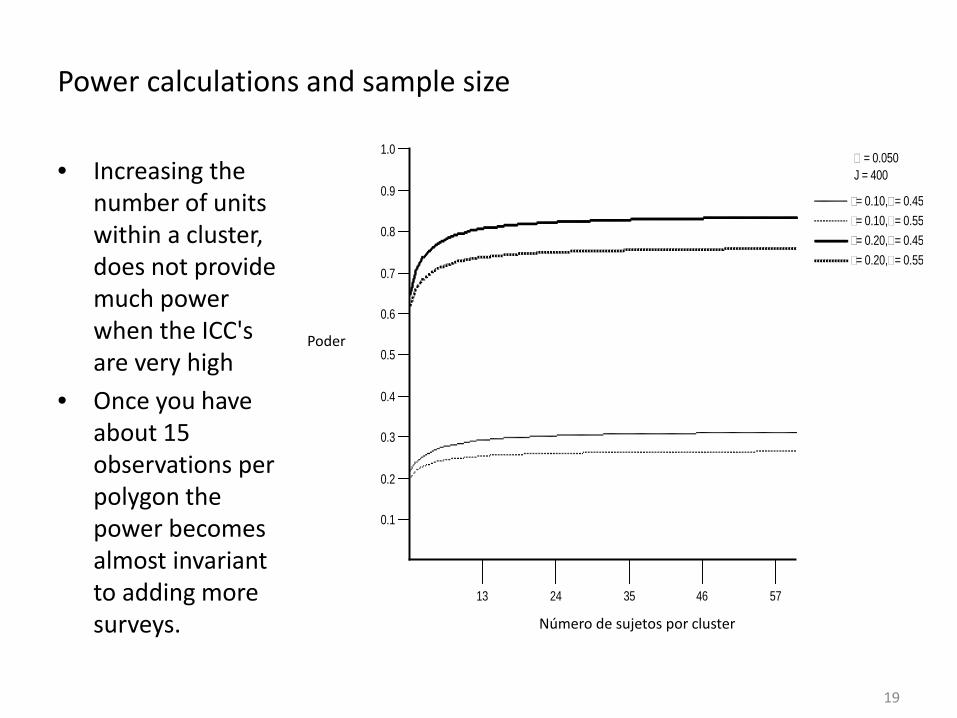
Power calculations and sample size
• Increasing the number of units within a cluster, does not provide much power when the ICC's are very high
• Once you have about 15 observations per polygon the power becomes almost invariant to adding more surveys.
Number of subjects per cluster
Power
13 24 35 46 57
0.1
0.2
0.3
0.4
0.5
0.6
0.7
0.8
0.9
1.0 = 0.050 J = 400
= 0.10,= 0.45= 0.10,= 0.55= 0.20,= 0.45= 0.20,= 0.55
Poder
Número de sujetos por cluster
20
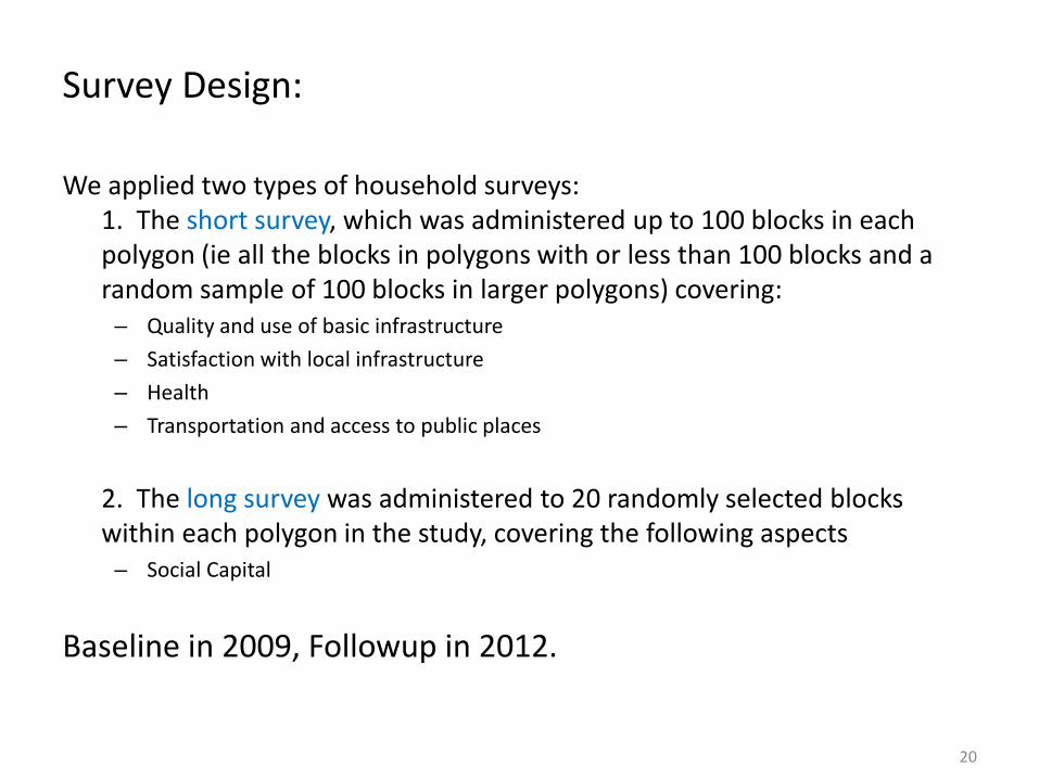
Survey Design:
We applied two types of household surveys: 1. The short survey, which was administered up to 100 blocks in each polygon (ie all the blocks in polygons with or less than 100 blocks and a random sample of 100 blocks in larger polygons) covering:
– Quality and use of basic infrastructure – Satisfaction with local infrastructure – Health – Transportation and access to public places
2. The long survey was administered to 20 randomly selected blocks within each polygon in the study, covering the following aspects
– Social Capital
Baseline in 2009, Followup in 2012.

21
Sample Selection:
• SEDESOL provided a sample of 19.427 blocks in 516 polygons with information from the 2005 Conteo; these sites were considered to be good candidates for expansion, in municipalities where they were confident that the program could work. Imposed some restrictions on the sample: 1. Not having cities with fewer than 4 polygons (in order to limit the number of distinct places in which they have to operate) 2. Not having municipalities with a single polygon in them (because the design included a randomization of the saturation at the level of. the municipalities). 3. SEDESOL could not work in 19 sites because they lacked confidence that they could control the intervention given prior relationships with local governments.
In the end we had 370 polygons in 68 municipalities and 33 cities. These contained 14.276 distinct blocks of which 11,387 ended up in the baseline household sample.
22
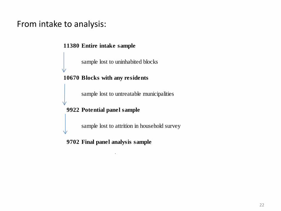
From intake to analysis:
11380 Entire intake sample
sample lost to uninhabited blocks
10670 Blocks with any residents
sample lost to untreatable municipalities
9922 Potential panel sample
sample lost to attrition in household survey
9702 Final panel analysis sample

23
Attrition:
Attrition looks fine at both municipality and block level. However, treated polygons have lower attrition at house level and much lower attrition at household level. Treatment reduces migration/churn? Core TEs are robust to looking at only stayers, but this is an issue. Question: Is this a block, a house, or a household study?
Baseline values of: (1) (2) (3) (4) (5) (6) (7) (8)Treatment -0.014 -0.00996 -0.00412 0.000965 -0.0363 -0.0297 -0.0874** -0.0737**
(0.048) (0.049) (0.005) (0.001) (0.030) (0.028) (0.042) (0.037)Index of Basic Services -0.00000749 -0.0000254 0.000614 0.000984
(0.001) (0.000) (0.000) (0.001)Satisfaction with Social Infrastructure 0.00166 -0.000922* -0.0029 0.00786
(0.008) (0.000) (0.005) (0.006)Observation Weight 0.0000488 -1.22e-05*** 0.000260* 0.000479**
(0.000) (0.000) (0.000) (0.000)
Average fraction attrited in control group:
# of Obs: 10,670 10,436 9,922 9,745 9,702 9,702 9,702 9,702
Attrition at Household level (baseline sampled household
replaced with alternate at followup)
0.176 0.388
Attrition Between Rounds 1 and 2:
Attrition at municipal level (municipality selected to be
part of study but removed by Habitat)
Attrition at block level (block sampled at baseline and in
study municipalities, but panel dependant variable not
observed)
0.095 0.016
Attrition at House level (baseline sampled house
replaced with alternate at followup)

24
Balance:
Study well-balanced overall. Use of randomized saturation design means that it looks very clean with municipal fixed-effects, less so without.
Balance Tests.
Average in Control Group
Treatment/ Control
Differential
Standard Error of Difference
# Households at Baseline
Piped Water 0.926 -0.0163 (0.016) 9,702Sewerage Service 0.829 -0.011 (0.027) 9,702Electric Lighting 0.989 -0.00884* (0.005) 9,702Use Water to Bathe 0.287 0.00801 (0.028) 8,649Flush Toilet 0.613 -0.0325 (0.023) 9,563Diarrea in Past 12 Months 0.178 -0.0169 (0.016) 9,702Street Lighting Always Works 0.555 -0.0255 (0.021) 9,702Street is Paved 0.664 0.0172 (0.025) 9,702Index of Basic Services 91.492 -1.204 (1.303) 9,702Index of Basic Infrastructure 68.512 1.097 (2.057) 9,702Availability of Services + Infrastructure 78.361 0.111 (1.506) 9,702Satisfaction with Physical Environment 2.844 -0.106 (0.084) 9,702Satisfaction with Social Environment 83.308 -2.320* (1.215) 9,702Knowledge of Public Programs 39.358 -1.322 (0.965) 9,702Regressions include fixed effects at the municipality level, and are weighted to be representative of all residents in the study neighborhoods. Standard Errors in parentheses are clustered at the polygon level to account for the design effect. Stars indicate significance at * 90%, ** 95%, and *** 99%.

25
Results: Infrastructure.
Piped WaterSewerage
ServiceElectric Lighting
Street Lights Medians Sidewalks Paved RoadsTrash
Collection
Index of Basic
Infrastructure
Satisfaction with Physical Infrastructure
Intention to Treat 0.00115 0.0203 0.00239 0.0607* 0.0617*** 0.0481** 0.0314** 0.00583 0.135*** 0.776*(0.016) (0.017) (0.005) (0.036) (0.021) (0.022) (0.014) (0.009) (0.048) (0.391)
Dummy for R2 0.0113* 0.0236** 0.00609* -0.00587 0.028 0.0428*** 0.0669*** 0.00701** 0.149*** -0.118(0.006) (0.012) (0.003) (0.033) (0.019) (0.015) (0.013) (0.003) (0.049) (0.379)
Baseline control mean: 0.926 0.829 0.989 0.555 0.588 0.589 0.664 0.971 2.740 8.825
Observations 684 684 684 682 684 684 684 684 684 684R-squared 0.013 0.053 0.029 0.021 0.092 0.11 0.209 0.018 0.161 0.027Number of polygons 342 342 342 342 342 342 342 342 342 342Polygon-level analysis with polygon fixed effects and standard errors clustered at the municipal level. Regressions weighted by polygon populations to make them representative of all inhabitants of study areas. Standard Errors in Parentheses, Stars indicate significance at * 90%, ** 95%, and *** 99%.
No impacts on water, sewerage, or electricity despite substantial overall improvements between 2009 and 2012. Very substantial impacts on street lights, paving, sidewalks, medians, an index of basic infrastructure, and reported satisfaction with physical infrastructure.

26
Robustness: Infrastructure:
Estimation Strategy:
Piped WaterSewerage
ServiceElectric Lighting
Street Lights Medians Sidewalks Paved RoadsTrash
Collection
Index of Basic
Infrastructure
Satisfaction with Physical Infrastructure
Round 2 Difference -0.0239 0.00395 0.00257 0.000774 0.0824*** 0.0747*** 0.0717*** -0.0127 0.224*** 0.285(0.015) (0.025) (0.002) (0.024) (0.026) (0.026) (0.020) (0.011) (0.071) (0.256)
Simple Diff-in-Diff 0.00185 0.0203 0.00244 0.0566* 0.0597*** 0.0478** 0.0317 0.0059 0.133** 0.754*(0.018) (0.019) (0.005) (0.034) (0.022) (0.021) (0.021) (0.010) (0.059) (0.387)
DiD w/ Municipality FE 0.00115 0.0217 0.00241 0.0548 0.0593*** 0.0467** 0.0299 0.00597 0.130** 0.776**(0.018) (0.019) (0.005) (0.034) (0.022) (0.022) (0.021) (0.010) (0.061) (0.384)
DiD w/ Block-level FE 0.00112 0.0205 0.00239 0.0570* 0.0619*** 0.0476** 0.0309 0.00596 0.135** 0.861**(0.018) (0.019) (0.005) (0.033) (0.023) (0.022) (0.021) (0.010) (0.061) (0.388)
Each cell denotes an impact estimated from a separate regression. Standard Errors in Parentheses, Stars indicate significance at * 90%, ** 95%, and *** 99%.
Dependent Variable:
To check robustness of main results, re-run at the household level using four additional specifications. As should be the case in a clean RCT, impacts are very robust to any estimation strategy, particularly all of those that are estimated in changes.
27
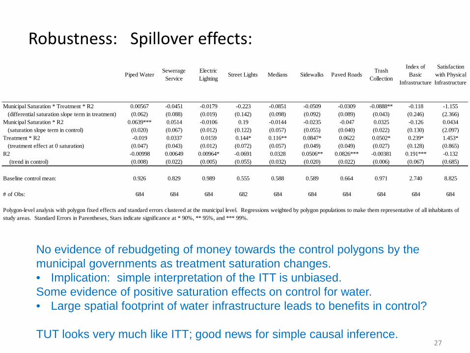
Robustness: Spillover effects:
No evidence of rebudgeting of money towards the control polygons by the municipal governments as treatment saturation changes. • Implication: simple interpretation of the ITT is unbiased. Some evidence of positive saturation effects on control for water. • Large spatial footprint of water infrastructure leads to benefits in control? TUT looks very much like ITT; good news for simple causal inference.
Piped WaterSewerage
ServiceElectric Lighting
Street Lights Medians Sidewalks Paved RoadsTrash
Collection
Index of Basic
Infrastructure
Satisfaction with Physical Infrastructure
Municipal Saturation * Treatment * R2 0.00567 -0.0451 -0.0179 -0.223 -0.0851 -0.0509 -0.0309 -0.0888** -0.118 -1.155 (differential saturation slope term in treatment) (0.062) (0.088) (0.019) (0.142) (0.098) (0.092) (0.089) (0.043) (0.246) (2.366)Municipal Saturation * R2 0.0639*** 0.0514 -0.0106 0.19 -0.0144 -0.0235 -0.047 0.0325 -0.126 0.0434 (saturation slope term in control) (0.020) (0.067) (0.012) (0.122) (0.057) (0.055) (0.040) (0.022) (0.130) (2.097)Treatment * R2 -0.019 0.0337 0.0159 0.144* 0.116** 0.0847* 0.0622 0.0502* 0.239* 1.453* (treatment effect at 0 saturation) (0.047) (0.043) (0.012) (0.072) (0.057) (0.049) (0.049) (0.027) (0.128) (0.865)R2 -0.00998 0.00649 0.00964* -0.0691 0.0328 0.0506** 0.0826*** -0.00381 0.191*** -0.132 (trend in control) (0.008) (0.022) (0.005) (0.055) (0.032) (0.020) (0.022) (0.006) (0.067) (0.685)
Baseline control mean: 0.926 0.829 0.989 0.555 0.588 0.589 0.664 0.971 2.740 8.825
# of Obs: 684 684 684 682 684 684 684 684 684 684
Polygon-level analysis with polygon fixed effects and standard errors clustered at the municipal level. Regressions weighted by polygon populations to make them representative of all inhabitants of study areas. Standard Errors in Parentheses, Stars indicate significance at * 90%, ** 95%, and *** 99%.

28
Results: Community Infrastructure.
Despite substantial expenditures on CDCs (27 treatment communities had investment in them) no reported overall increase in existence or use. Increases in access to libraries. No improvement in health outcomes. No improvement in travel times Almost-significant improvement in satisfaction with social environment.
Community Development Center Exists
Community Development Center Used
Park ExistsLibrary Exists
Sports facilities
Exist
Taken local Trainings/ courses
Household Member ill in past 3 months
Household Member
Tested past 3 months
Index of Travel Time to Facilities
Satisfaction with Social
Environment
treat_r2 -0.00206 -0.00481 0.0476 0.0442** 0.0223 0.0148 0.062 -0.227 -0.00549 0.357(0.038) (0.015) (0.050) (0.020) (0.044) (0.021) (0.038) (0.144) (0.033) (0.259)
r2 0.042 0.0227 0.0386 0.0148 0.0389 0.00254 -0.0901** 0.182 -0.0369 -0.702***(0.032) (0.014) (0.036) (0.017) (0.034) (0.013) (0.036) (0.125) (0.029) (0.239)
Baseline control mean: 0.168 0.053 0.319 0.149 0.434 0.121 0.371 1.245 -0.002 7.642
Observations 684 684 684 684 684 684 684 684 684 684R-squared 0.026 0.027 0.054 0.039 0.029 0.005 0.059 0.02 0.022 0.109Number of polygons 342 342 342 342 342 342 342 342 342 342Polygon-level analysis with polygon fixed effects and standard errors clustered at the municipal level. Regressions weighted by polygon populations to make them representative of all inhabitants of study areas. Standard Errors in Parentheses, Stars indicate significance at * 90%, ** 95%, and *** 99%.
29
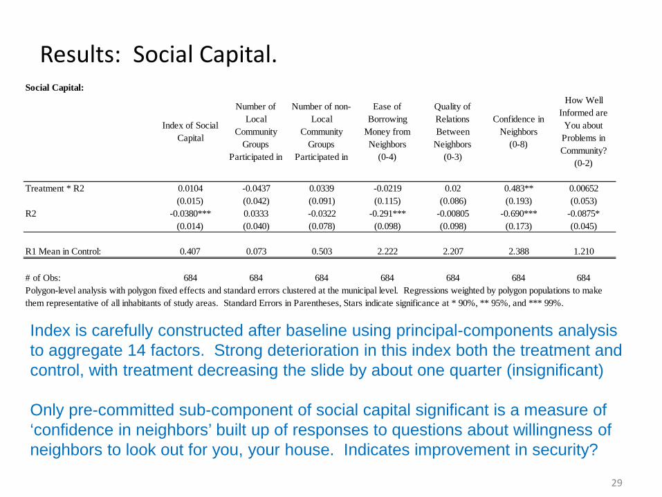
Results: Social Capital.
Index is carefully constructed after baseline using principal-components analysis to aggregate 14 factors. Strong deterioration in this index both the treatment and control, with treatment decreasing the slide by about one quarter (insignificant) Only pre-committed sub-component of social capital significant is a measure of ‘confidence in neighbors’ built up of responses to questions about willingness of neighbors to look out for you, your house. Indicates improvement in security?
Social Capital:
Index of Social Capital
Number of Local
Community Groups
Participated in
Number of non-Local
Community Groups
Participated in
Ease of Borrowing
Money from Neighbors
(0-4)
Quality of Relations Between
Neighbors (0-3)
Confidence in Neighbors
(0-8)
How Well Informed are
You about Problems in Community?
(0-2)
Treatment * R2 0.0104 -0.0437 0.0339 -0.0219 0.02 0.483** 0.00652 (0.015) (0.042) (0.091) (0.115) (0.086) (0.193) (0.053)R2 -0.0380*** 0.0333 -0.0322 -0.291*** -0.00805 -0.690*** -0.0875* (0.014) (0.040) (0.078) (0.098) (0.098) (0.173) (0.045)
R1 Mean in Control: 0.407 0.073 0.503 2.222 2.207 2.388 1.210
# of Obs: 684 684 684 684 684 684 684Polygon-level analysis with polygon fixed effects and standard errors clustered at the municipal level. Regressions weighted by polygon populations to make them representative of all inhabitants of study areas. Standard Errors in Parentheses, Stars indicate significance at * 90%, ** 95%, and *** 99%.

30
Results: Crime.
All point estimates negative, substantial drop in the probability of being assaulted; strong enough to overcome the horrible trend in the control. Results need to be interpreted against a background of rapidly-deteriorating security in the country 2009-2012.
Crime:
Any Household Member Victim of Crime in past
12 mos?
Any Household Member
Assaulted in Street in past 12
mos?
Number of Activities
Abandoned Due to Insecurity
(0-8)
Number of Issues over which Intra-Community
Conflict (0-12)
Treatment * R2 -0.0484 -0.152** -0.249 -0.0373 (0.044) (0.067) (0.345) (0.297)R2 0.0483 0.125** 0.536* -0.0876 (0.031) (0.055) (0.312) (0.254)
R2 Mean in Control: 0.106 0.096 2.682 1.332
# of Obs: 684 684 684 684Polygon-level analysis with polygon fixed effects and standard errors clustered at the municipal level. Regressions weighted by polygon populations to make them representative of all inhabitants of study areas. Standard Errors in Parentheses, Stars indicate significance at * 90%, ** 95%, and *** 99%.

31
Results: Youth behavior.
These results were not a part of the baseline pre-analysis plan, but show a range of interesting effects. Since both CDCs and Social and Community Development spending are heavily focused at improving educational outlets for youth, these are encouraging. People haven’t heard of CDCs but report their kids getting precisely the services provided there.
Youth Problems:
Number of Problems Faced
by Youth in Community (0-9)
Youth Lack Cultural/Artistic
Facilities?
Gang Activity is a Problem for
Youth?
Alcohol/Drugs are a Problem
for Youth?
Youth Get Together to Play Sports/Music?
Youth Get Together to
Fight Between Groups?
Youth Get Together to
Beg?
Treatment * R2 -0.382* -0.0877** -0.0978* -0.0558** 0.166*** -0.119** -0.0984* (0.201) (0.037) (0.052) (0.025) (0.057) (0.051) (0.057)Treat 0.172 0.0402* 0.0382 0.0268 -0.0650* 0.0529 0.0312 (0.127) (0.024) (0.031) (0.018) (0.037) (0.037) (0.037)R2 0.0462 0.0484 0.00765 0.0387** -0.157*** 0.0992*** 0.0262 (0.152) (0.032) (0.046) (0.018) (0.046) (0.035) (0.050)
R1 Mean in Control: 6.491 0.801 0.719 0.788 0.482 0.495 0.318
# of Obs: 11,075 11,132 11,124 11,135 5,040 5,038 5,036Household-level analysis with municipal fixed effects and standard errors clustered at the polygon level. Regressions weighted by block-level populations to make them representative of all inhabitants of study areas. Standard Errors in Parentheses, Stars indicate significance at * 90%, ** 95%, and *** 99%.

32
Does public investment crowd in private investment?
Wide range of private investment indicators show improvement. This includes indicators such as use of flush toilets and (inferior) septic systems that are related to broader investments, but also things like concrete flooring that appear to have no direct connection. Rents are going up: Sign of improvement in property prices?
Private Investment, analysis at Polygon level.
Brick WallsConcrete
FloorsSeparate Kitchen
Separate Bathroom
Flush ToiletSeptic
SystemPiped Water Home Owner
Private Bank Mortgage
Monthly Rent (for renters
only)
treat_r2 0.00337 0.0229** 0.0112 0.00416 0.0707** -0.0273** 0.0146 0.0208 0.00962 218.8*(0.008) (0.009) (0.016) (0.014) (0.031) (0.013) (0.023) (0.022) (0.006) (127.200)
r2 0.00763 0.00743 0.0307** 0.0184** -0.0475* 0.00162 0.0628*** 0.00557 -0.0134** -8.751(0.006) (0.005) (0.012) (0.008) (0.025) (0.012) (0.015) (0.009) (0.005) (94.150)
Baseline control mean: 0.942 0.965 0.876 0.930 0.608 0.113 0.703 0.844 0.019 1159.8
Observations 684 684 684 684 684 684 684 684 683 530R-squared 0.012 0.065 0.089 0.033 0.037 0.014 0.105 0.019 0.034 0.047Number of polygons 342 342 342 342 342 342 342 342 342 299Polygon-level analysis with polygon fixed effects and standard errors clustered at the municipal level. Regressions weighted by polygon populations to make them representative of all inhabitants of study areas. Standard Errors in Parentheses, Stars indicate significance at * 90%, ** 95%, and *** 99%.

33
Impacts on real estate values:
Sharp improvements in property prices analyzed in a variety of different ways. Distribution of prices in treatment first-order stochastic dominates distribution in the control.
Simple DID
Weighting by number of
viviendas per observation
Including municipality
Fixed Effects
Clustering Standard
Errors at the Polygon level
Treatment effect 62.22*** 69.78** 70.79** 70.79** (15.320) (32.990) (31.100) (35.650)Constant -2.537 42.69** -232.9*** -232.9***
(10.050) (20.340) (40.480) (54.710)
Observations 437 437 437 437R-squared 0.037 0.033 0.371 0.371
Analysis at the Polygon level:
Simple DID
Weighting by number of
viviendas per observation
Including municipality
Fixed Effects
Treatment effect 72.06** 69.78* 70.79* (28.070) (37.980) (42.090)Constant 16.1 42.69** -232.9***
(18.660) (21.580) (64.590)
Observations 138 138 138R-squared 0.046 0.037 0.418
Dependent Variable: Changes in real estate price per square meter, real 2012 pesos.
0.2
.4.6
.81
-200 0 200 400 600 800Price change 2009-2012
Treatment Polygons Control Polygons
Polygon-level averages
Real 2012 peso increases per square meterCDFs of Property Price Changes, by Treatment

34
Discussion of real estate price impacts:
Weaknesses: 1. Although this sample is the universe of unbuilt lots for sale in all study
polygons at baseline, sample is only 437 lots, located in only 138 polygons (40% of the original sample).
2. The sub-sample with sales not representative of the study; lots with sales have worse physical capital and better social capital.
Strengths: 1. The experiment is very well-balanced within this sample. 2. We have professional property valuations provided by INDAABIN. 3. INDAABIN valuators were blinded to the research design. 4. Use of unbuilt lots avoids confounding with the improvements in the
quality of the housing stock. Upshot: every peso invested in a polygon led to two pesos in the total value of real estate in the polygon. Evidence of under-supply of infrastructure.
35
How to estimate impacts on voting behavior?
Mexico’s Federal Electoral Institute (IFE) provides most disaggregated data at the precinct level (143,437 precints and 66,826 secciones in the country).
Take shapefile of seccion boundaries, overlay this onto the maps of the Hábitat polygons.
Calculate the share of each polygon that is in each seccion, use these shares as weights to collapse up voting totals and then compare the vote shares for the incumbent
Electoral outcomes exist for races at the presidential (national), senatorial (state), and deputy (regional) level.
Hypotheses: 1. With attribution to national spending, program should have increased vote
share for incumbent PAN party in presidential election. We test this. 2. With attribution to local spending, program should have increased the re-
election probability of the incumbent party at the municipal level. We are still working on this.

36
Political Impacts: Attribution
Heard of Habitat
Heard of non-Habitat
programs
Benefited from Habitat
Benefitted from non-Habitat programs
Treatment * R2 0.0765*** 0.244 -0.000558 -0.00892 (0.027) (0.497) (0.004) (0.071)Treat -0.0267 -0.281 0.000881 -0.0567 (0.017) (0.316) (0.002) (0.053)R2 -0.0994*** -1.641*** 0.00309 -0.0281 (0.022) (0.452) (0.003) (0.052)
R2 Mean in Control: 0.115 7.602 0.008 0.753
# of Obs: 19,417 19,417 19,417 14,394
Standard Errors in Parentheses, Stars indicate significance at * 90%, ** 95%, and *** 99%.
People have heard of Hábitat more in treatment polygons, but are no more likely to think they have benefitted from the program!

37
Political Impacts: Voting in the 2012 elections.
No evidence of benefit experienced by PAN in presidential election. Consistent with complete lack of ability of respondents to attribute improvements correctly to Hábitat.
Voting outcomes
Share voting for PAN
Share voting for PRI
Share voting for PAN
Share voting for PRI
Share voting for PAN
Share voting for PRI
Treatment Effect 0.00135 0.000976 -0.00106 0.000322 -0.0016 0.00344(0.005) (0.005) (0.005) (0.005) (0.005) (0.006)
Mean in Control group 0.217 0.280 0.229 0.294 0.228 0.294
Observations 341 341 341 341 341 341R-squared 0.876 0.82 0.886 0.832 0.878 0.832
Presidential (National) Election
Senatorial (State) Election
Diputado (Municipal) Election

38
How to perform analysis at block-level?
We have information at the block level, but randomization was conducted at the polygon level. Then the polygon level can be thought of as an analysis of "intent to treat (ITT) and try to understand the impact on real blocks treated as the effect of treatment on the treated (TOT). It is necessary to find non-experimental methods for the analysis despite the randomization at polygon level. One option is to perform propensity score matching block level Estimate. Predict. Pick blocks in control polygons that are most like those in intervention polygons that actually receive Hábitat investment, and compare them.
While the comparison is not directly experimental, we have a perfectly comparable control group from which to pick counterfactuals.
More interesting, policy-relevant quantity than the ITT of this type of hybrid program. Also, since TOT effects presumably stronger, may be more powerful way to look at social capital impacts.
0Pr( 1) 1ib ib ib iX u Tτ β β= = + + ∀ =0
ˆ ˆˆPr( 1) 0ib ib iX Tτ β β= = + ∀ =

39
Moving towards the ToT:
(1) (2) (3)
OLS OLSOLS w/ FE for
deciles of propensity score
ITT -1.103 (1.593)ToT of Road Paved -4.398*** -4.527*** (1.695) (1.718)
# of Obs: 5,508 3,489 3,460
Time to Reach Closest Market, in Minutes.
Regressions include fixed effects at the municipality level, and are weighted to be representative of all residents in the study neighborhoods. Standard Errors in parentheses are clustered at the polygon level to account for the design effect. Stars indicate significance at * 90%, ** 95%, and *** 99%.
01
23
4
0 .2 .4 .6 .8x
All Treatment All ControlActually Treated
Propensity to have Road Paved by HabitatDensities of Propensity score, by group
Leaves the territory of experimental identification. Requires ‘selection on observables’ assumption, but randomized control means you have the entire counterfactual distribution: common support for sure. So far effective propensity score has been difficult to build; working on pushing the ‘buffers’ around the location of infrastructure to be smaller. Should provide more pin-point form of the ToT.
40
Conclusions. Analysis of largest randomized experiment in Mexico since Progresa. • Substantial impacts on the infrastructure to which most of the money went. • Little observable impact of spending on water, sewer, electricity. • Mixed results on social capital; participation doesn’t improve but treated
neighborhoods appear more secure, provide more youth services. • Large effects on private investment, value of privately held real estate. • Absolutely no evidence of correct attribution, let alone political benefits of
program. – Contrary to Gonzales-Navarro & Quintana-Domeque (2011), who find increased support for
local politicians from road building in Veracruz. • Why no impacts on health? Indoor plumbing and concrete floors both
improve. – Cattaneo et al. (2009) show getting rid of dirt floors decreases diarrhea in Mexico, but Klasen et
al. (2012) show that increasing piped water in Yemen led to increase. • Is estimate of $2 in value for every $1 in spending reasonable?
– Estimates in US range from $.65 (Pereira and Flores de Frutos 1999) to $1.50 (Cellini et al. 2010), Mexico more constrained, so this may not be a crazy number.
Overall takeaway: public spending creates substantial private value, large improvements in localized infrastructure, more mixed improvements for social and human capital.