10.1 pore pressures, landslides, - hwbhydrogeologistswithoutborders.org/wordpress/wp... · 10.1...

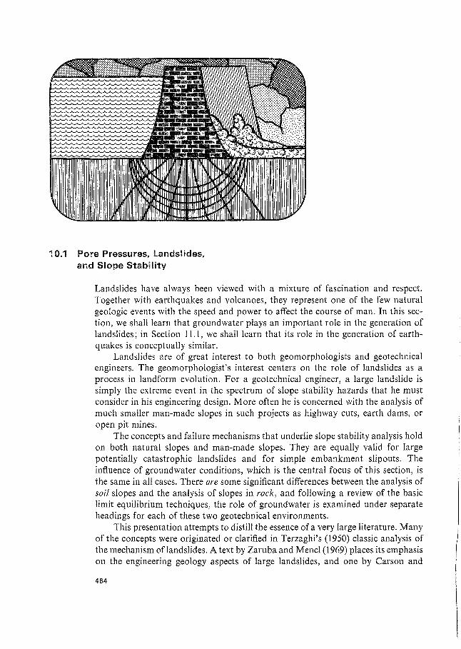
10.1 Pore Pressures, landslides, and Slope Stability

Landslides have always been viewed with a mixture of fascination and respect. Together with earthquakes and volcanoes, they represent one of the few natural geologic events with the speed and power to affect the course of man. In this section, we shall learn that groundwater plays an important role in the generation of landslides; in Section 11.1, we shall learn that its role in the generation of earthquakes is conceptually similar.

Landslides are of great interest to both geomorphologists and geotechnical engineers. The geomorphologisf s interest centers on the role of landslides as a process in landform evolution. For a geotechnical engineer, a large landslide is simply the extreme event in the spectrum of slope stability hazards that he must consider in his engineering design. More often he is concerned with the analysis of much smaller man-made slopes in such projects as highway cuts, earth dams, or open pit mines.

The concepts and failure mechanisms that underlie slope stability analysis hold on both natural slopes and man-made slopes. They are equally valid for large potentially catastrophic landslides and for simple embankment slipouts. The influence of groundwater conditions, which is the central focus of this section, is the same in all cases. There are some significant differences between the analysis of soil slopes and the analysis of slopes in rock, and following a review of the basic limit equilibrium techniques, the role of groundwater is examined under separate headings for each of these two geotechnical environments.

This presentation attempts to distill the essence of a very large literature. Many of the concepts were originated or clarified in Terzaghi's (1950) classic analysis of the mechanism of landslides. A text by Zaruba and Mencl (1969) places its emphasis on the engineering geology aspects of large landslides, and one by Carson and

464

465 Groundwater and Geotechnical Problems / Ch. 10

Kirkby (1972) reviews the geomorphological implications. Eckel (1958), Coates (1977), and Schuster and Krizek (in press) provide a comprehensive review of slope-stability engineering, and a recent text by Hoek and Bray (1974) emphasizes rock slope engineering. Standard soil mechanics texts such as Terzaghi and Peck (1967) treat the subject in some detail. Throughout the literature there is generous recognition of the importance of fluid pressures, but this recognition is not always coupled with an up-to-date understanding of the probable patterns of steady-state and transient subsurface flow in slopes.

We will begin with an examination of the mechanisms of subsurface movement on planar surfaces.

Mohr-Coulomb Failure Theory

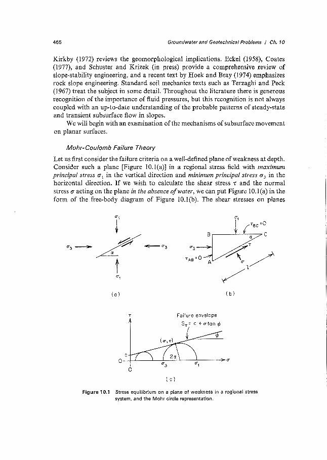
Let us first consider the failure criteria on a well-defined plane of weakness at depth. Consider such a plane [Figure 10.l(a)] in a regional stress field with maximum principal stress u 1 in the vertical direction and minimum principal stress u 3 in the horizontal direction. If we wish to calculate the shear stress 7: and the normal stress u acting on the plane in the absence of water, we can put Figure 10.I(a) in the form of the free-body diagram of Figure 10. l (b ). The shear stresses on planes

0"1

i r 'sc =O

/--~, B

0"3~ 0"3__,....

t 0"1

(al ( b)

T Failure envelope

S,= c + o-ton <f:i

0

( c)

Figure 10.1 Stress equilibrium on a plane of weakness in a regional stress system, and the Mohr circle representation.

c

466 Groundwater and Geotechnica/ Problems / Ch. 10

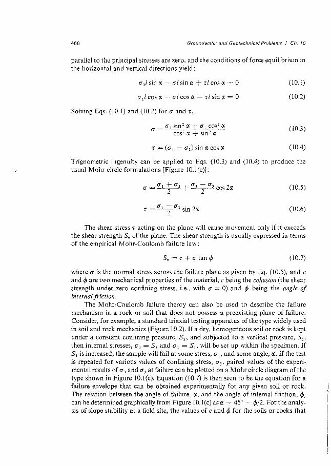
parallel to the principal stresses are zero, and the conditions of force equilibrium in the horizontal and vertical directions yield:

a) sin a - al sin a+ rl cos a= 0

a 1 l cos a -- al cos a - r/ sin a = 0

Solving Eqs. (10.1) and (10.2) for a and r,

a = a 3 sin 2 a + a 1 cos 2 a cos2 a+ sin 2 a

(10.l)

(10.2)

(10.3)

(10.4)

Trignometric ingenuity can be applied to Eqs. (10.3) and (10.4) to produce the usual Mohr circle formulations [Figure 10. l (c)]:

(10.5)

(10.6)

The shear stress r acting on the plane will cause movement only if it exceeds the shear strength Sr of the plane. The shear strength is usually expressed in terms of the empirical Mohr-Coulomb failure law:

S-r = c + a tan ¢ (10.7)

where a is the normal stress across the failure plane as given by Eq. (10.5), and c and¢ are two mechanical properties of the material, c being the cohesion (the shear strength under zero confining stress, i.e., with a = 0) and ¢ being the angle of internal friction.

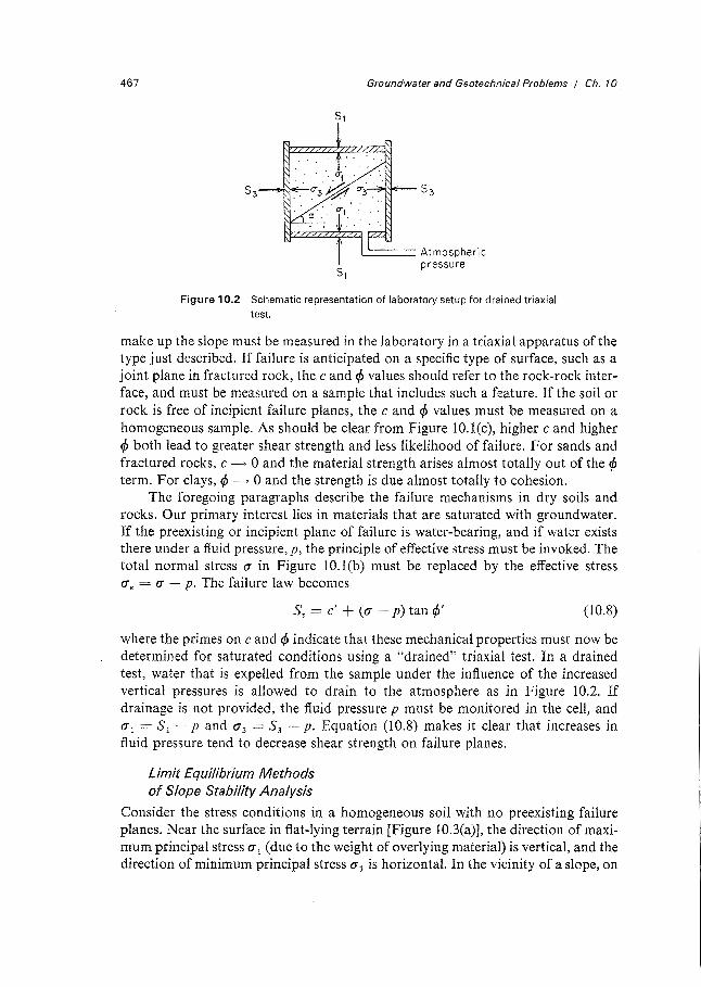
The Mohr-Coulomb failure theory can also be used to describe the failure mechanism in a rock or soil that does not possess a preexisting plane of failure. Consider, for example, a standard triaxial testing apparatus of the type widely used in soil and rock mechanics (Figure 10.2). If a dry, homogeneous soil or rock is kept under a constant confining pressure, S3 , and subjected to a vertical pressure, S 1,

then internal stresses, a 3 = S 3 and a 1 = S 1 , will be set up within the specimen. If S 1 is increased, the sample will fail at some stress, a 1 , and some angle, a. If the test is repeated for various values of confining stress, a 3 , paired values of the experimental results of a 3 and a 1 at failure can be plotted on a Mohr circle diagram of the type shown in Figure 10.l(c). Equation (10.7) is then seen to be the equation for a failure envelope that can be obtained experimentally for any given soil or rock. The relation between the angle of failure, a, and the angle of internal friction, ¢, can be determined graphically from Figure 10.l(c) as a= 45° - <f>/2. For the analysis of slope stability at a field site, the values of c and¢ for the soils or rocks that


.___ ___ Atmospheric pressure

Figure 10.2 Schematic representation of laboratory setup for drained triaxial test.

make up the slope must be measured in the laboratory in a triaxial apparatus of the type just described. If failure is anticipated on a specific type of surface, such as a joint plane in fractured rock, the c and <f.> values should refer to the rock-rock interface, and must be measured on a sample that includes such a feature. If the soil or rock is free of incipient failure planes, the c and <f.> values must be measured on a homogeneous sample. As should be clear from Figure 10.l(c), higher c and higher <f.> both lead to greater shear strength and less likelihood of failure. For sands and fractured rocks, c --" 0 and the material strength arises almost totally out of the <f.>

term. For clays, <f.> --" 0 and the strength is due almost totally to cohesion. The foregoing paragraphs describe the failure mechanisms in dry soils and

rocks. Our primary interest lies in materials that are saturated with groundwater. If the preexisting or incipient plane of failure is water-bearing, and if water exists there under a fluid pressure, p, the principle of effective stress must be invoked. The total normal stress a in Figure 10.l(b) must be replaced by the effective stress ae = a - p. The failure law becomes

ST = c' + (a - p) tan <f.>' (10.8)

where the primes on c and <f.> indicate that these mechanical properties must now be determined for saturated conditions using a "drained" triaxial test. In a drained test, water that is expelled from the sample under the influence of the increased vertical pressures is allowed to drain to the atmosphere as in Figure 10.2. If drainage is not provided, the fluid pressure p must be monitored in the cell, and a 1 = S 1 - p and a3 = S 3 - p. Equation (10.8) makes it clear that increases in fluid pressure tend to decrease shear strength on failure planes.

limit Equilibrium Methods of Slope Stability Analysis

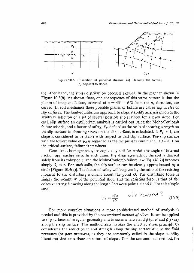
Consider the stress conditions in a homogeneous soil with no preexisting failure planes. Near the surface in flat-lying terrain [Figure 10.3(a)], the direction of maximum principal stress a 1 (due to the weight of overlying material) is vertical, and the direction of minimum principal stress a 3 is horizontal. In the vicinity of a slope, on


{a) ( b)

Figure 10.3 Orientation of principal stresses. (a) Beneath flat terrain; (b) adjacent to slopes.

the other hand, the stress distribution becomes skewed, in the manner shown in Figure 10.3(b). As shown there, one consequence of this stress pattern is that the planes of incipient failure, oriented at a = 45° - <f>/2 from the u 3 direction, are curved. In soil mechanics these possible planes of failure are called slip circles or slip surfaces. The limit-equilibrium approach to slope stability analysis involves the arbitrary selection of a set of several possible slip surfaces for a given slope. For each slip surface an equilibrium analysis is carried out using the Mohr-Coulomb failure criteria, and a factor of safety, F8 , defined as the ratio of shearing strength on the slip surface to shearing stress on the slip surface, is calculated. If Fs > 1, the slope is considered to be stable with respect to that slip surface. The slip surface with the lowest value of Fs is regarded as the incipient failure plane. If Fs < I on the critical surface, failure is imminent.

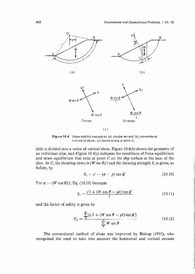
Consider a homogeneous, isotropic clay soil for which the angle of internal friction approaches zero. In such cases, the shear strength of the soil is derived solely from its cohesion c, and the Mohr-Coulomb failure law [Eq. (10.7)] becomes simply Sr: = c. For such soils, the slip surface can be closely approximated by a circle [Figure 10.4(a)]. The factor of safety will be given by the ratio of the resisting moment to the disturbing moment about the point 0. The disturbing force is simply the weight W of the potential slide, and the resisting force is that of the cohesive strength c acting along the length l between points A and B. For this simple case,

Wd Fs=clr

(10.9)

For more complex situations a more sophisticated method of analysis is needed and this is provided by the conventional method of slices. It can be applied to slip surfaces of irregular geometry and to cases where c and <f> (or c' and </>') vary along the slip surface. This method also invokes the effective stress principle by considering the reduction in soil strength along the slip surface due to the fluid pressures (or pore pressures, as they are commonly called in the slope stability literature) that exist there on saturated slopes. For the conventional method, the


(a)

W cosB

Forces

( c)

( b)

W cosB 1

Stresses

Figure 10.4 Slope stability analysis by (a) circular arc and (b) conventional method of slices; (c) forces acting at point C.

slide is divided into a series of vertical slices. Figure 10.4(b) shows the geometry of an individual slice, and Figure 10.4(c) indicates the conditions of force equilibrium and stress equilibrium that exist at point C on the slip surface at the base of the slice. At C, the shearing stress is ( W sin ())/I and the shearing strength S"' is given, as before, by

Sr = c' + (a - p) tan ¢'

For a= (W cos())/!, Eq. (IO.IO) becomes

S = c'l + (W cos() - pl) tan¢' -c l

and the factor of safety is given by

B

~ [c'l + (W cos() - pl) tan¢'] Fs = A B

~ Wsin () A

(IO.IO)

(10.11)

(10.12)

The conventional method of slices was improved by Bishop (1955), who recognized the need to take into account the horizontal and vertical stresses


produced along the slice boundaries due to the interactions between one slice and another. The resulting equation for Fs is somewhat more complicated than Eq. (10.12), but it is of the same form. [Carson and Kirkby (1972) present a simple derivation.] Bishop and Morgenstern (1960) produced sets of charts and graphs that simplify the application of the Bishop method of slices. Morgenstern and Price (1965) generalized the Bishop approach even further, and their technique for irregular slopes and general slip surfaces in nonhomogeneous media has been widely computerized. Computer packages for the routine analysis of complex slope stability problems are now in wide use.

To apply the limit equilibrium method to a given slope, whether by computer or by hand, the basic approach is to measure c' and ¢' for the slope material, calculate W, l, 8, and p for the various slices, and calculate Fs for the various slip surfaces under analysis.

Of all the required data, probably the most sensitive is the pore pressure p along the potential sliding planes. If economics permit, it may be possible to install piezometers in the slope at the depth of the anticipated failure plane. The measured hydraulic heads, h, can then be converted to pore pressures by means of the usual relationship:

p = pg(h - z) (10.13)

where z is the elevation of the piezometer intake . .In many cases, however, field instrumentation is not feasible, and it behooves us to reexamine the hydrogeology of slopes in light of the needs of slope stability analysis.

Effect of Groundwater Conditions on Slope Stability in Soils

The hydraulic heads (and pore pressures) on a slope reflect the steady-state or transient groundwater flow system that exists there. From the considerations of Chapter 6, it should be clear that if reasonable estimates can be made of the watertable configuration and of the distribution of soil types, it should be possible to predict the pore pressure distributions along potential slip surfaces by means of flow-net construction or with the aid of analytical, numerical, or analog simulation.

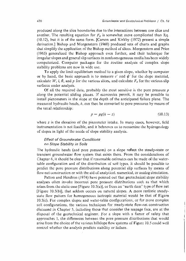
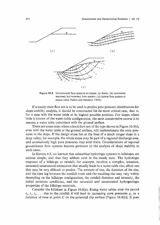
Patton and Hendron (1974) have pointed out that geotechnical slope stability analyses often invoke incorrect pore pressure distributions such as that which arises from the static case [Figure 10.5(a)], or from an "earth dam" type of flow net [Figure 10.5(b )], that seldom occurs on natural slopes. A more realistic steadystate flow pattern for homogeneous isotropic material would be that of Figure 10.5(c). For complex slopes and water-table configurations, or for more complex soil configurations, the various techniques for steady-state flow-net construction discussed in Chapter 5, including those that consider the seepage face, are at the disposal of the geotechnical engineer. For a slope with a factor of safety that approaches 1, the differences between the pore pressure distributions that would arise from the choice of the various hillslope flow systems of Figure 10.5 could well control whether the analysis predicts stability or failure.


(a) ( b)

( c)

Figure 10.5 Groundwater flow systems on slopes. (a) Static; (b) commonly assumed, but incorrect, flow system; (c) typical flow system in slopes (after Patton and Hendron, 1974).

If a steady-state flow net is to be used to predict pore pressure distributions for slope-stability analysis, it should be constructed for the most critical case, that is, for a case with the water table at its highest possible position. For slopes where little is known of the water-table configuration, the most conservative course is to assume a water table coincident with the ground surface.

There are some cases where a local flow net of the type shown in Figure 10.5(c), even with the water table at the ground surface, will underestimate the pore pressures in the slope. If the design slope lies at the base of a much longer slope in a deep valley, for example, the whole slope may be part of a regional discharge area, and anomalously high pore pressures may exist there. Considerations of regional groundwater flow systems become pertinent to the analysis of slope stability in such cases.

In Section 6.5, we learned that subsurface hydrologic systems in hillslopes are seldom simple, and that they seldom exist in the steady state. The hydrologic response of a hillslope to rainfall, for example, involves a complex, transient, saturated-unsaturated interaction that usually leads to a water-table rise, albeit one that may be very difficult to predict. The amount of rise, the duration of the rise, and the time lag between the rainfall event and the resulting rise may vary widely depending on the hillslope configuration, the rainfall duration and intensity, the initial moisture conditions, and the saturated and unsaturated hydrogeologic properties of the hillslope materials.

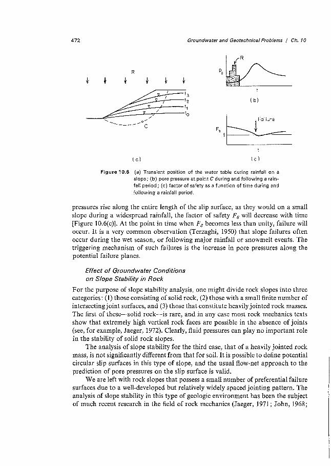
Consider the hillslope in Figure 10.6(a). Rising water tables over the period t 0 , t 1, t 2 , • • • due to the rainfall R will lead to increasing pore pressures pc as a function of time at point C on the potential slip surface [Figure 10.6(b)]. If pore

472 Groundwater and Geotechnica/ Problems I Ch. 10

R

( b)

(a) ( c)

Figure 10.6 (a) Transient position of the water table during rainfall on a slope; (b) pore pressure at point C during and following a rainfall period; (c) factor of safety as a function of time during and following a rainfall period.

pressures rise along the entire length of the slip surface, as they would on a small slope during a widespread rainfall, the factor of safety F8 will decrease with time [Figure 10.6(c)]. At the point in time when F8 becomes less than unity, failure will occur. It is a very common observation (Terzaghi, 1950) that slope failures often occur during the wet season, or following major rainfall or snowmelt events. The triggering mechanism of such failures is the increase in pore pressures along the potential failure planes.

Effect of Groundwater Conditions on Slope Stability in Rock

For the purpose of slope stability analysis, one might divide rock slopes into three categories: (1) those consisting of solid rock, (2) those with a small finite number of intersecting joint surfaces, and (3) those that constitute heavily jointed rock masses. The first of these-solid rock-is rare, and in any case most rock mechanics texts show that extremely high vertical rock faces are possible in the absence of joints (see, for example, Jaeger, 1972). Clearly, fluid pressures can play no important role in the stability of solid rock slopes.

The analysis of slope stability for the third case, that of a heavily jointed rock mass, is not significantly different from that for soil. It is possible to define potential circular slip surfaces in this type of slope, and the usual flow-net approach to the prediction of pore pressures on the slip surface is valid.

We are left with rock slopes that possess a small number of preferential failure surfaces due to a well-developed but relatively widely spaced jointing pattern. The analysis of slope stability in this type of geologic environment has been the subject of much recent research in the field of rock mechanics (Jaeger, 1971; John, 1968;


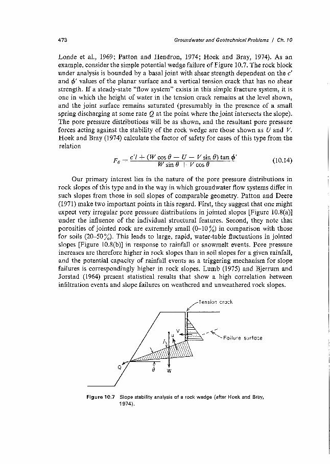
Londe et al., 1969; Patton and Hendron, 1974; Hoek and Bray, 1974). As an example, consider the simple potential wedge failure of Figure 10.7. The rock block under analysis is bounded by a basal joint with shear strength dependent on the c' and <P' values of the planar surface and a vertical tension crack that has no shear strength. If a steady-state "flow system" exists in this simple fracture system, it is one in which the height of water in the tension crack remains at the level shown, and the joint surface remains saturated (presumably in the presence of a small spring discharging at some rate Q at the point where the joint intersects the slope). The pore pressure distributions will be as shown, and the resultant pore pressure forces acting against the stability of the rock wedge are those shown as U and V. Hoek and Bray (1974) calculate the factor of safety for cases of this type from the relation

F = c' l + ( W cos 0 - U - V sin 0) tan <P' s w sin 0 + v cos e (10.14)

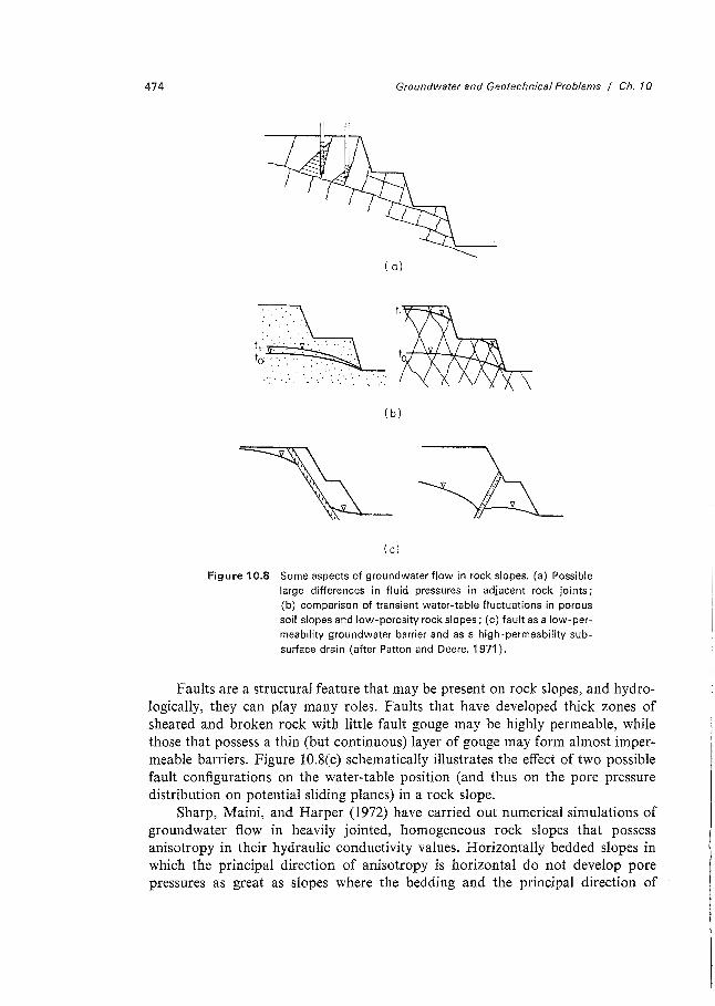
Our primary interest lies in the nature of the pore pressure distributions in rock slopes of this type and in the way in which groundwater flow systems differ in such slopes from those in soil slopes of comparable geometry. Patton and Deere (1971) make two important points in this regard. First, they suggest that one might expect very irregular pore pressure distributions in jointed slopes [Figure 10.8(a)] under the influence of the individual structural features. Second, they note that porosities of jointed rock are extremely small (0-10%) in comparison with those for soils (20-50 %). This leads to large, rapid, water-table fluctuations in jointed slopes [Figure 10.8(b )] in response to rainfall or snowmelt events. Pore pressure increases are therefore higher in rock slopes than in soil slopes for a given rainfall, and the potential capacity of rainfall events as a triggering mechanism for slope failures is correspondingly higher in rock slopes. Lumb (1975) and Bjerrum and Jorstad (1964) present statistical results that show a high correlation between infiltration events and slope failures on weathered and unweathered rock slopes.

/Tension crock

,...----.

8 w

figure 10.7 Slope stability analysis of a rock wedge (after Hoek and Bray, 1974).

474 Groundwater and Geotechnica! Problems I Ch. 10

(a)

( b)

( c)

Figure 10.8 Some aspects of groundwater flow in rock slopes. (a) Possible large differences in fluid pressures in adjacent rock joints; (b) comparison of transient water-table fluctuations in porous soil slopes and low-porosity rock slopes; {c) fault as a low-per

meability groundwater barrier and as a high-permeability sub

surface drain (after Patton and Deere, 1971 ).

Faults are a structural feature that may be present on rock slopes, and hydrologically, they can play many roles. Faults that have developed thick zones of sheared and broken rock with little fault gouge may be highly permeable, while those that possess a thin (but continuous) layer of gouge may form almost impermeable barriers. Figure 10.8(c) schematically illustrates the effect of two possible fault configurations on the water-table position (and thus on the pore pressure distribution on potential sliding planes) in a rock slope.

Sharp, Maini, and Harper (1972) have carried out numerical simulations of groundwater flow in heavily jointed, homogeneous rock slopes that possess anisotropy in their hydraulic conductivity values. Horizontally bedded slopes in which the principal direction of anisotropy is horizontal do not develop pore pressures as great as slopes where the bedding and the principal direction of


anisotropy dip parallel to the slope face. The very large divergence in the hydraulic head distribution that they show between the two cases illustrates the importance of a detailed understanding of the hydrogeological regime on a slope for the purposes of stability analysis.

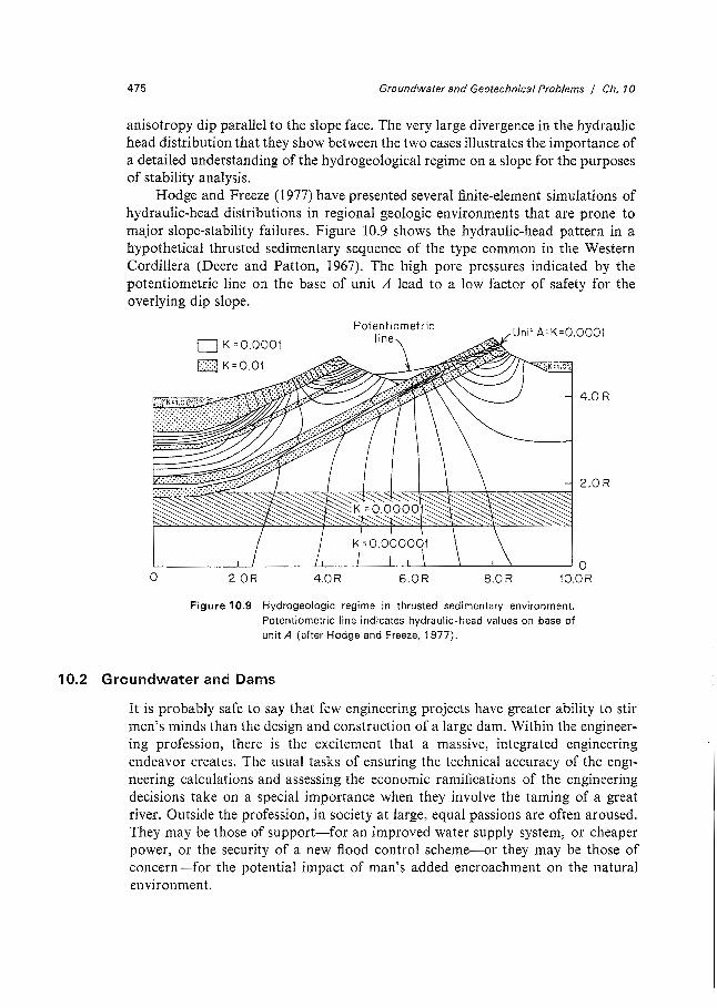
Hodge and Freeze (1977) have presented several finite-element simulations of hydraulic-head distributions in regional geologic environments that are prone to major slope-stability failures. Figure 10.9 shows the hydraulic-head pattern in a hypothetical thrusted sedimentary sequence of the type common in the Western Cordillera (Deere and Patton, 1967). The high pore pressures indicated by the potentiometric line on the base of unit A lead to a low factor of safety for the overlying dip slope.

D K=0.0001

D K=0.01

Unit A: K=0.0001

4.0 R

2.0R

'--~~~~_..__,_~~~-'-'-~--'-~----'-~~~~~~~~~~~ 0 0 2.0R 4.0R 6.0R 8.0R 10.0R

Figure 10.9 Hydrogeologic regime in thrusted sedimentary environment. Potentiometric line indicates hydraulic-head values on base of unit A (after Hodge and Freeze, 1977).

10.2 Groundwater and Dams

It is probably safe to say that few engineering projects have greater ability to stir men's minds than the design and construction of a large dam. Within the engineering profession, there is the excitement that a massive, integrated engineering endeavor creates. The usual tasks of ensuring the technical accuracy of the engineering calculations and assessing the economic ramifications of the engineering decisions take on a special importance when they involve the taming of a great river. Outside the profession, in society at large, equal passions are often aroused. They may be those of support-for an improved water supply system, or cheaper power, or the security of a new flood control scheme-or they may be those of concern-for the potential impact of man's added encroachment on the natural environment.


The engineering concerns are usually centered on the damsite, and in the first part of this section we will look at the role of groundwater in the engineering aspects of dam design. The environmental concerns are more often associated with the reservoir, and in the later part of the section we will examine the environmental interactions that take place between an artificially impounded reservoir and the regional hydrogeologic regime.

Types of Dams and Dam Failures

No two dams are exactly alike. Individual dams differ in their dimensions, design, and purpose. They differ in the nature of the site they occupy and in the size of the reservoir they impound. One obvious initial classification would separate large multipurpose dams, few in number but great in impact, from the much larger number of smaller structures such as tailings dams, coffer dams, floodwalls, and overflow weirs. In this presentation the role of groundwater is examined in the context of the larger dams, but the principles are equally applicable to the smaller structures.

Krynine and Judd (1957) classify large dams into four categories: gravity dams, slab and buttress dams, arch dams, and earth and rockfill dams. The first' three represent impermeable concrete structures that do not permit the percolation of water through them or the buildup of pore pressures within them. These three are differentiated on the basis of their geometry and by the mechanisms through which they transfer the water loads to their foundations. A gravity dam has an axis that extends across a valley from one abutment to the other in a straight line, or very nearly so. Its structural cross section is massive, usually trapezoidal, but approaching a triangle in some cases. A slab-and-buttress dam has a cross section that is considerably thinner than a full gravity dam, but one that is buttressed by a set of vertical walls aligned at right angles to the dam axis. An arch dam has a curved axis, its convex face upstream. In the most spectacular cases, its section may be little more than a reinforced concrete wall, often less than 20 ft thick. In a gravity dam, the water load is transmitted to the foundations through the dam itself; in a buttress dam the load is transmitted through the buttresses; and in an arch dam the load is transmitted to the rock abutments by the thrusting action of the arch. All three types of concrete dam must be founded on rock, and the role of subsurface water is thus limited to the groundwater flow and pore pressure development that can occur in the abutment rocks and in the rock foundations.

In the first half of this century, most of the earth's large dams were contructed as concrete dams on rock foundations. However, in recent years, as the better damsites have become exhausted and the economic trade-off between the costs of concrete construction and the cost of earthmoving has changed, there has been a sweeping move toward earth and rockfill dams. These dams derive their stability from a massive cross section and as a result they can be built at almost any site, on either rock or soil foundations. From a hydro logic point of view, the primary property that differentiates earth dams from concrete dams is that they are perme-


able to some degree. They allow a limited flow of water through their cross section and they permit the development of pore pressures within their mass.

There are essentially five events that can lead to a catastrophic dam failure: (I) overtopping of the dam by a flood wave due to insufficient spillway capacity, (2) movement within the rock foundations or abutments on planes of geological weakness, (3) the development of large uplift pressures on the base of the dam, ( 4) piping at the dam toe, and (5) slope failures on the upstream or downstream face of the dam. The first three of these failure mechanisms can occur in both concrete and earth dams; the last two are limited to earth and rockfill dams.

There is also a sixth mode of failure-excessive leakage from the reservoirthat is seldom catastrophic but which represents just as serious a breakdown in design as any of the first five. Of course, leakage always takes place to some degree through the foundation rocks beneath a dam, and in earth dams, there is always some loss through the dam itself. These losses are usually carefully analyzed during the design of a dam. Losses that are unexpected more often take place through the abutment rocks or from the reservoir at some point distant from the dam. There are even a few case histories (Krynine and Judd, 1957) that report leakage so excessive that the dams were effectively unable to hold water. Engineers need methods of prediction for the rates of leakage, great or small, because leakage values are an important part of the hydrologic balance on which cost-benefit analyses of dams are based.

The presence of groundwater is a typical feature at damsites. Of the six modes of failure we have listed, groundwater plays an important role in five of themgeological failure, uplift failure, piping failure, slope failure, and leakage failure. Under the next few headings we will examine the various failure mechanisms in more detail, and we will look at some of the design features that are incorporated in dams to provide safeguards against failure. For the first section, which deals with concrete dams on rock foundations, Jaeger (1972), Krynine and Judd (1957), and Legget (1962) provide useful reference texts. For the discussions that deal with earth and rockfill dams, the specialty texts of Sherard et al. (1963) and Cedergren (1967) are invaluable. A recent book by Wahlstrom (1974) on damsite exploration techniques contains much material of hydrogeologic interest.

Seepage Under Concrete Dams

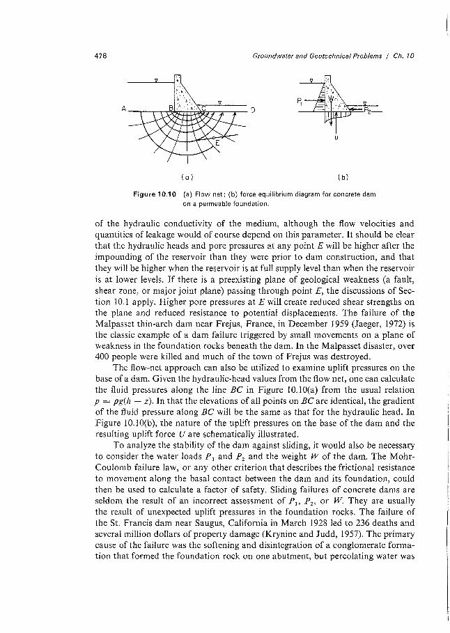
In order to examine the failure mechanisms on geological planes of weakness, consider the cross section of Figure 10.IO(a) through an impermeable, concrete, gravity dam and its underlying rock foundation. If the elevation of the reservoir level on the upstream side of the dam is h 1 and the elevation of the tailwater pond on the downstream side of the dam is h2 , a steady-state flow net can be constructed in the infinite half-space on the basis of the boundary conditions h = h1 on AB, h = h2 on CD, and BC impermeable. The flow net shown in Figure 10.lO(a) is for a homogeneous, isotropic medium. The hydraulic heads, pressure heads, and fluid pressures (or pore pressures) that exist at any point in the system are independent

478 Groundwater and Geotechnical Problems I Ch. 10

u

( 0) ( b)

Figure 10.10 (a) Flow net; (b) force equilibrium diagram for concrete dam on a permeable foundation.

of the hydraulic conductivity of the medium, although the flow velocities and quantities of leakage would of course depend on this parameter. It should be clear that the hydraulic heads and pore pressures at any point E will be higher after the impounding of the reservoir than they were prior to dam construction, and that they will be higher when the reservoir is at fu11 supply level than when the reservoir is at lower levels. If there is a preexisting plane of geological weakness (a fault, shear zone, or major joint plane) passing through point E, the discussions of Section 10.1 apply. Higher pore pressures at E will create reduced shear strengths on the plane and reduced resistance to potential displacements. The failure of the Malpasset thin-arch dam near Frejus, France, in December 1959 (Jaeger, 1972) is the classic example of a dam failure triggered by small movements on a plane of weakness in the foundation rocks beneath the dam. In the Malpasset disaster, over 400 people were killed and much of the town of Frejus was destroyed.

The flow-net approach can also be utilized to examine uplift pressures on the base of a dam. Given the hydraulic-head values from the flow net, one can calculate the fluid pressures along the line BC in Figure 10. lO(a) from the usual relation p = pg(h - z). In that the elevations of all points on BC are identical, the gradient of the fluid pressure along BC will be the same as that for the hydraulic head. In Figure I 0.1 O(b ), the nature of the uplift pressures on the base of the dam and the resulting uplift force U are schematically illustrated.

To analyze the stability of the dam against sliding, it would also be necessary to consider the water loads P 1 and P2 and the weight W of the dam. The MohrCoulomb failure law, or any other criterion that describes the frictional resistance to movement along the basal contact between the dam and its foundation, could then be used to calculate a factor of safety. Sliding failures of concrete dams are seldom the result of an incorrect assessment of P 1, P2 , or W. They are usually the result of unexpected uplift pressures in the foundation rocks. The failure of the St. Francis dam near Saugus, California in March 1928 led to 236 deaths and several million dollars of property damage (Krynine and Judd, 1957). The primary cause of the failure was the softening and disintegration of a conglomerate formation that formed the foundation rock on one abutment, but percolating water was


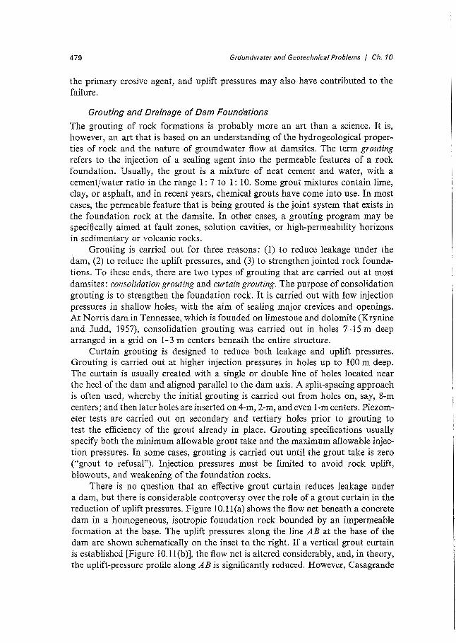
the primary erosive agent, and uplift pressures may also have contributed to the failure.

Grouting and Drainage of Dam Foundations

The grouting of rock formations is probably more an art than a science. It is, however, an art that is based on an understanding of the hydrogeological properties of rock and the nature of groundwater flow at damsites. The term grouting refers to the injection of a sealing agent into the permeable features of a rock foundation. Usually, the grout is a mixture of neat cement and water, with a cement/water ratio in the range 1 : 7 to 1 : 10. Some grout mixtures contain lime, clay, or asphalt, and in recent years, chemical grouts have come into use. In most cases, the permeable feature that is being grouted is the joint system that exists in the foundation rock at the damsite. In other cases, a grouting program may be specifically aimed at fault zones, solution cavities, or high-permeability horizons in sedimentary or volcanic rocks.

Grouting is carried out for three reasons: (1) to reduce leakage under the dam, (2) to reduce the uplift pressures, and (3) to strengthen jointed rock foundations. To these ends, there are two types of grouting that are carried out at most damsites: consolidation grouting and curtain grouting. The purpose of consolidation grouting is to strengthen the foundation rock. It is carried out with low injection pressures in shallow holes, with the aim of sealing major crevices and openings. At Norris dam in Tennessee, which is founded on limestone and dolomite (Krynine and Judd, 1957), consolidation grouting was carried out in holes 7-15 m deep arranged in a grid on 1-3 m centers beneath the entire structure.

Curtain grouting is designed to reduce both leakage and uplift pressures. Grouting is carried out at higher injection pressures in holes up to 100 m deep. The curtain is usually created with a single or double line of holes located near the heel of the dam and aligned parallel to the dam axis. A split-spacing approach is often used, whereby the initial grouting is carried out from holes on, say, 8-m centers; and then later holes are inserted on 4-m, 2-m, and even 1-m centers. Piezometer tests are carried out on secondary and tertiary holes prior to grouting to test the efficiency of the grout already in place. Grouting specifications usually specify both the minimum allowable grout take and the maximum allowable injection pressures. In some cases, grouting is carried out until the grout take is zero ("grout to refusal"). Injection pressures must be limited to avoid rock uplift, blowouts, and weakening of the foundation rocks.

There is no question that an effective grout curtain reduces leakage under a dam, but there is considerable controversy over the role of a grout curtain in the reduction of uplift pressures. Figure 10.l l(a) shows the flow net beneath a concrete dam in a homogeneous, isotropic foundation rock bounded by an impermeable formation at the base. The uplift pressures along the line AB at the base of the dam are shown schematically on the inset to the right. If a vertical grout curtain is established [Figure 10.1 l(b)], the flow net is altered considerably, and, in theory, the uplift-pressure profile along AB is significantly reduced. However, Casagrande


(a)

A B

( b) L ( c)

( d)

( e)

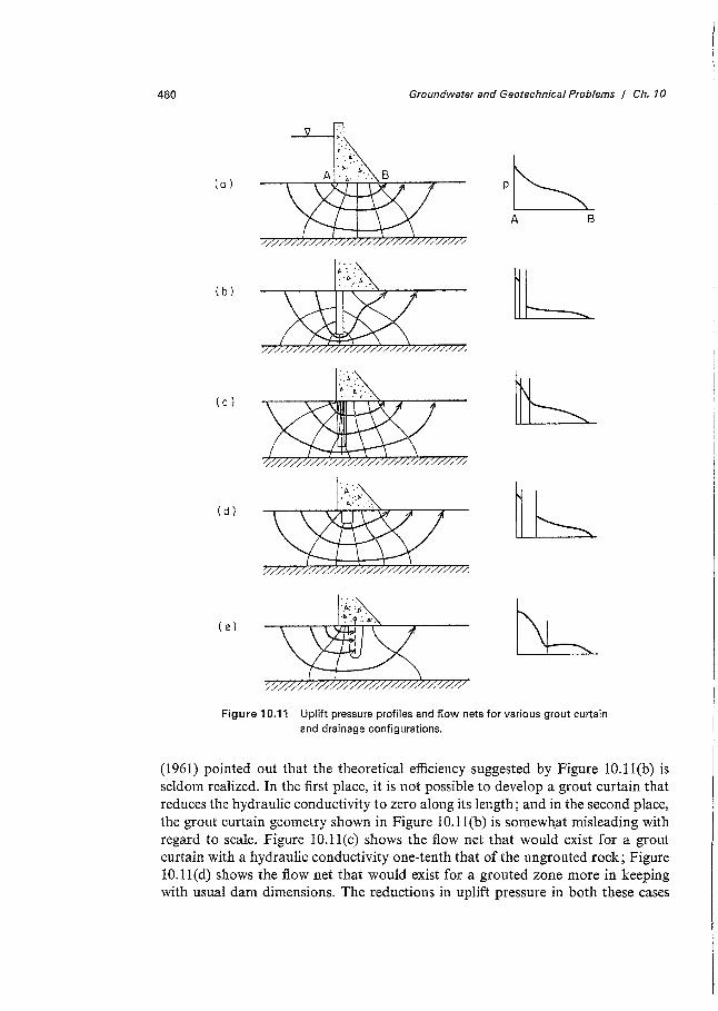
Figure 10.11 Uplift pressure profiles and flow nets for various grout curtain and drainage configurations.

( 1961) pointed out that the theoretical efficiency suggested by Figure 10.11 (b) is seldom realized. In the first place, it is not possible to develop a grout curtain that reduces the hydraulic conductivity to zero along its length; and in the second place, the grout curtain geometry shown in Figure 10.ll(b) is somewhat misleading with regard to scale. Figure 10.ll(c) shows the flow net that would exist for a grout curtain with a hydraulic conductivity one-tenth that of the ungrouted rock; Figure 10.ll(d) shows the flow net that would exist for a grouted zone more in keeping with usual dam dimensions. The reductions in uplift pressure in both these cases


is significantly less than that shown in Figure 10.11 (b ). Casagrande notes that uplift pressures are actually more effectively reduced by drainage [Figure 10.l l(e)]. However, the presence of a drain induces even greater leakage from the reservoir than would occur under natural conditions. It is common practice now to use an integrated design with a grout curtain to reduce leakage and drainage behind the curtain to reduce uplift pressures.

The Grand Rapids hydroelectric project in Manitoba provides a grouting case history second to none (Grice, 1968; Rettie and Patterson, 1963). The project involved 25 km of earth dikes, enclosing a reservoir greater than 5000 km2 in area, in a region underlain by highly fractured dolomites. A grout curtain up to 70 m in depth was emplaced from holes on less than 2-m centers over the entire length of the dikes. Grice (1968) notes that the grout curtain reduced leakage through the grouted formation by 83 %, but it induced greater flows through the underlying ungrouted rock. He estimates that the grouting program reduced net leakage from the reservoir by 63 %.

Steady-State Seepage Through Earth Dams

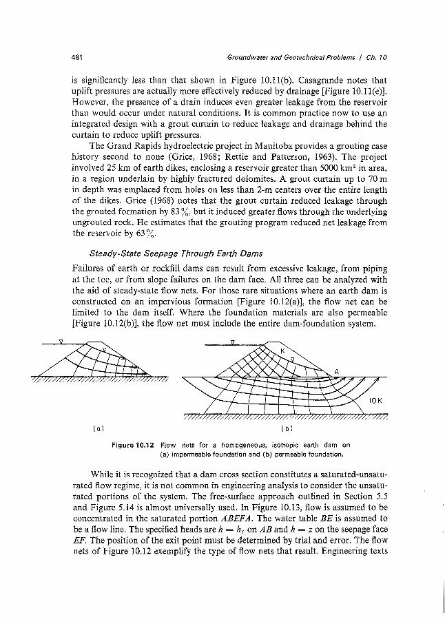
Failures of earth or rockfill dams can result from excessive leakage, from piping at the toe, or from slope failures on the dam face. All three can be analyzed with the aid of steady-state flow nets. For those rare situations where an earth dam is constructed on an impervious formation [Figure 10.12(a)], the flow net can be limited to the dam itself. Where the foundation materials are also permeable [Figure 10.12(b )J, the flow net must include the entire dam-foundation system.

(a) ( b)

Figure 10.12 Flow nets for a homogeneous, isotropic earth dam on (a) impermeable foundation and (b) permeable foundation.

While it is recognized that a dam cross section constitutes a saturated-unsaturated flow regime, it is not common in engineering analysis to consider the unsaturated portions of the system. The free-surface approach outlined in Section 5.5 and Figure 5.14 is almost universally used. In Figure 10.13, flow is assumed to be concentrated in the saturated portion ABEFA. The water table BE is assumed to be a flow line. The specified heads are h = h 1 on AB and h = z on the seepage face EF. The position of the exit point must be determined by trial and error. The flow nets of Figure 10.12 exemplify the type of flow nets that result. Engineering texts


Figure 10.13 Boundary-value problem for saturated-unsaturated flow system in earth dam.

on groundwater seepage such as Harr (1962) or Cedergren (1967) provide many examples of flow nets for earth dams.

Let us now consider the question of piping. The mechanism of piping can be explained in terms of the forces that exist on an individual soil grain in a porous medium during flow. The flow of water past the soil grain occurs in response to an energy gradient. (Recall from Section 2.2 that the hydraulic potential was defined in terms of the energy per unit mass of flowing fluid.) A measure of this gradient is provided by the difference in hydraulic head .D.h between the front and back faces of the grain. The force that acts on the grain due to the differential head is known as the seepage force. It is exerted in the direction of flow and can be calculated (Cedergren, 1967) from the expression

F= pg MA (10.15)

where A is the cross-sectional area of the grain and pis the mass density of water. If we multiply Eq. (10.15) by .D.z/.D.z and let A refer to a cross-sectional area that encompasses many grains, we have an expression for the seepage force during vertical flow through a unit volume of porous media with V = A .D.z = I. Putting the resulting expression in differential form yields

ah F =pg az (10.16)

The seepage force is therefore directly proportional to the hydraulic gradient ah/az. In areas of downward-percolating groundwater, the seepage forces act in the same direction as the gravity forces, but in areas of upward-flowing water, they oppose the gravity forces. If the upward-directed seepage force at any discharge point in a flow system [say, at point A in Figure 10.12(b)] exceeds the downwarddirected gravity force, piping will occur. Soil grains will be carried away by the discharging seepage and the dam will be undermined.

The downward-directed gravity force is due to the buoyant weight of the saturated porous medium. A soil with a dry density Ps = 2.0 g/cm3 has a buoyant density (pb = Ps - p) that is almost exactly equal to the density of water, p = 1.0 g/cm3 • For this very representative Ps value, the seepage force will exceed the gravity force for all hydraulic gradients greater than 1.0. One simple test for piping


is therefore to examine the flow net for a proposed dam design and calculate the hydraulic gradients at all discharge points. If there are exit gradients that approach 1.0, an improved design is required.

The ultimate failure mode in cases of piping is usually a slope failure on the downstream face. Slope failures can also occur there if the pore pressures created near the face by the internal flow system are too great. The limit equilibrium methods of slope stability analysis, introduced in the previous section, are just as applicable to earth dams as they are to natural slopes.

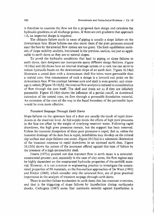
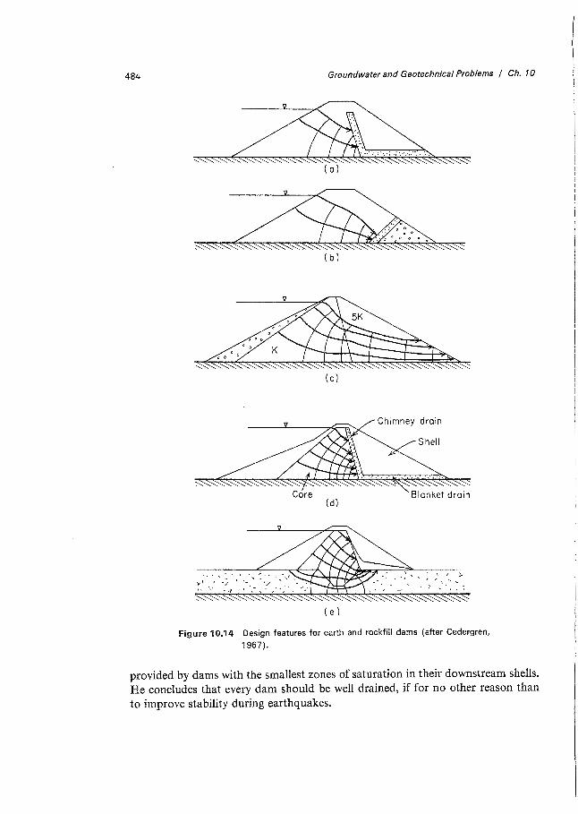
To avoid the hydraulic conditions that lead to piping or slope failures in earth dams, dam designers can incorporate many different design features. Figure 10.14(a) and (b) shows how an internal drainage system or a rock toe can serve to reduce hydraulic heads on the downstream slope of an earth dam. Figure 10.14(c) illustrates a zoned dam with a downstream shell five times more permeable than a central core. One consequence of such a design is a lowered exit point on the downstream face. If the contrast between core and shell is even greater, and drainage is added, [Figure 10. I 4( d)], the internal flow analysis is reduced to consideration of flow through the core itself. The shell and drain act as if they are infinitely permeable. Figure I 0.14( e) shows the influence of a partial cutoff, or downward extension of the central core, on flow through a permeable foundation material. An extension of the core all the way to the basal boundary of the permeable layer would be even more effective.

Transient Seepage Through Earth Dams

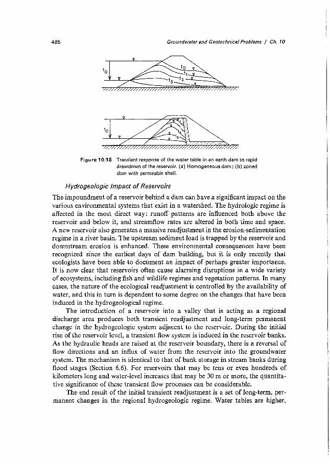
Slope failures on the upstream face of a dam are usually the result of rapid drawdowns in the reservoir level. At full supply levels the effects of high pore pressures in the face are offset by the weight of overlying reservoir water. Following rapid drawdown, the high pore pressures remain, but the support has been removed. Unless the transient dissipation of these pore pressures is rapid, that is, unless the transient drainage of the dam face is rapid, instabilities may develop on the critic3;1 slip surface and slope failures can occur. Figure 10.15(a) is a schematic illustration of the transient response to rapid drawdown in an unzoned earth dam. Figure 10.15(b) shows the nature of the insurance offered against this type of failure by the presence of a high-permeability shell.

Freeze (197la) pointed out that transient flow in earth dams is a saturatedunsaturated process; and, especially in the case of clay cores, the flow regime may be highly dependent on the unsaturated hydraulic properties of the earthfill material. However, it is not common in engineering practice to investigate the unsaturated properties of fill materi~ls, so the free-surface approaches of De Wiest (1962) and Dicker (1969), which consider only the saturated flow, are of great practical importance in the analysis of transient seepage through earth dams.

There is another failure mechanism in earth dams that has transient overtones, and that is the triggering of slope failures by liquefaction during earthquake shocks. Cedergren (1967) notes that maximum security against liquefaction is


.: 0 0 • • ~ 0

~ •• (} Q " 0 " ~~ ~

, • 0

. , 0

( b)

~ 5K

o o a .:i K

~ ~ (c)

( e)

Figure 10.14 Design features for earth and rockfill dams (after Cedergren,

1967).

provided by dams with the smallest zones of saturation in their downstream shells. He concludes that every dam should be well drained, if for no other reason than to improve stability during earthquakes.


:! v.

Figure 10.15 Transient response of the water table in an earth dam to rapid drawdown of the reservoir. (a) Homogeneous dam; (b) zoned dam with permeable shell.

Hydrogeologic Impact of Reservoirs

The impoundment of a reservoir behind a dam can have a significant impact on the various environmental systems that exist in a watershed. The hydrologic regime is affected in the most direct way: runoff patterns are influenced both above the reservoir and below it, and streamflow rates are altered in both time and space. A new reservoir also generates a massive readjustment in the erosion-sedimentation regime in a river basin. The upstream sediment load is trapped by the reservoir and downstream erosion is enhanced. These environmental consequences have been recognized since the earliest days of dam building, but it is only recently that ecologists have been able to document an impact of perhaps greater importance. It is now clear that reservoirs often cause alarming disruptions in a wide variety of ecosystems, including fish and wildlife regimes and vegetation patterns. In many cases, the nature of the ecological readjustment is controlled by the availability of water, and this in turn is dependent to some degree on the changes that have been induced in the hydrogeological regime.

The introduction of a reservoir into a valley that is acting as a regional discharge area produces both transient readjustment and long-term permanent change in the hydrogeologic system adjacent to the reservoir. During the initial rise of the reservoir level, a transient flow system is induced in the reservoir banks. As the hydraulic heads are raised at the reservoir boundary, there is a reversal of flow directions and an influx of water from the reservoir into the groundwater system. The mechanism is identical to that of bank storage in stream banks during flood stages (Section 6.6). For reservoirs that may be tens or even hundreds of kilometers long and water-level increases that may be 30 m or more, the quantitative significance of these transient flow processes can be considerable.

The end result of the initial transient readjustment is a set of long-term, permanent changes in the regional hydrogeologic regime. Water tables are higher,


hydraulic heads are increased in aquifers, and the rates of discharge from the subsurface flow system into the valley are reduced. If water-table elevations prior to impoundment were low, a regional water-table rise can be beneficial in that improved moisture conditions in near-surface soils may aid agricultural production. On the other hand, if water-table levels were already close to the surface, the influence may be harmful. Soils may become waterlogged, and there is the possibility of soil salinization through increased evaporation. In deeper aquifers, increased hydraulic heads will reduce pumping lifts and in rare situations can cause wells to flow that previously had static levels below the ground surface.

The preliminary analyses that lead to a reservoir design should include predictions of hydrogeologic impact. The predictive methods of simulation currently in use have largely been adapted from the methods of analysis of bank storage. The initial transient response of the water table can be modeled with a saturated model based on the Dupuit-Forchheimer assumptions (Hornberger et al., 1970) or with a more complex saturated-unsaturated analysis (Verma and Brutsaert, 1970). Transient increases in hydraulic head in a hydraulically connected confined aquifer can be predicted with the subsurface portion of Pinder and Sauer's (1971) coupled model of streamflow-aquifer interaction. All these methods require knowledge of the time rate of fluctuation of reservoir stage and the saturated and/ or unsaturated hydrogeologic properties of the geologic formations in the vicinity of the reservoir. Similar methods can be used to predict hydrogeologic response to operating fluctuations in reservoir level. This application has much in common with the assessment of transient flow through earth dams, as discussed earlier in this section.

Once a reservoir has attained its operating level, seasonal and operational fluctuations in water level are usually relatively small in comparison with the initial rise, and transient effects become less important. Prediction of long-term, permanent changes in the hydrogeologic regime can be carried out with a steady-state model, in which the head on the reservoir boundary is taken as the full supply level of the reservoir. Simulations can be performed on vertical two-dimensional cross sections aligned at right angles to the reservoir axis, or in two-dimensional horizontal cross sections through specific aquifers. Solutions are usually obtained numerically with the aid of a computer (Remson et al., 1965) or with analog models of the type described in Section 5.2 (van Everdingen, 1968a).

If the presence of a reservoir influences the hydrogeologic environment, so does the hydrogeologic environment influence a reservoir. In the eyes of a dam designer, the question of interaction is framed in the latter sense. In addition to the primary question of hydrologic supply and the secondary question of sedimentation in the reservoir, dam designers must consider three potential geotechnical problems in connection with reservoir design: (1) leakage from the reservoir at points other than the dam itself, (2) slope stability of the reservoir banks, and (3) earthquake generation. Each of these phenomena is influenced by groundwater conditions, either directly or through pore pressure effects.

Leakage from reservoirs at points distant from the dam is not uncommon.


It was a recurring problem in several of the dams constructed in limestone terrain by the Tennessee Valley Authority during the first half of this century.

The slope stability of reservoir banks, particularly under conditions of fluctuating water levels, is an important aspect of dam design. This has been especially true since the spectacular failure of the Vaiont reservoir in Italy in 1963. At that site a massive slide into the reservoir involving 200-300 million m 3 of material created a wave 250 m high that overtopped the dam and delivered 300 million m 3

of water into the downstream valley. Jaeger (1972) reports that almost 2500 lives were lost in the disaster.

The impoundment of a reservoir also changes the stress conditions at depth. The water load of the reservoir increases the total stresses, and this effect, together with the increase in fluid pressures brought about by hydrogeologic readjustment, influences effective stresses at depth. Carder (1970) documents a large number of case histories where reservoir impoundment has led to seismic activity.

10.3 Groundwater Inflows Into Tunnels

There is probably no engineering project that requires a more compatible marriage between geology and engineering than the construction of a tunnel. Consideration of the local and regional lithology, stratigraphy, and geologic structure influence not only the choice of routes but also the methods of excavation and support. A recent text by Wahlstrom (1973) outlines the history and development of tunneling and emphasizes the role of geology in tunnel planning. Krynine and Judd (1957) and Legget (1962) provide informative but less-detailed discussions of tunneling within the context of an overall treatment of engineering geology.

The tunneling literature contains references to many case histories in a wide variety of geologic environments, but while lithology, stratigraphy, and structure vary from case to case, there is one feature that is remarkably common. In case after case, the primary geotechnical problem encountered during tunnel construction involved the inflow of groundwater. Some of the most disastrous experiences in tunneling have been the result of interception of large flows of water from highly fractured, water-saturated rocks. Tunnelers the world over know that in planning for a tunnel it is essential to make every attempt to identify the nature of the groundwater conditions that are likely to be encountered.

If groundwater inflows are predicted in advance, it is usually possible to design suitable drainage systems. Where tunnels can be driven upgrade, the tunnel itself provides a primary drainage facility. Where tunnels must be driven downgrade or from internal headings serviced by a shaft, more complex drainage facilities involving pumps and piping systems are required. In either case, the requirements of design make it an important task to correctly predict the amounts and rates of water inflow that are likely to appear in the tunnel. In some cases it has proven possible to reduce groundwater inflows after the fact by grouting, but this approach is seldom of value when very large, unexpected inflows occur.


In this section we will first examine the role that a tunnel plays within the regional hydrogeologic system. In later subsections we will describe two famous case histories, and we will review some methods of predictive analysis.

A Tunnel as a Steady-State or Transient Drain

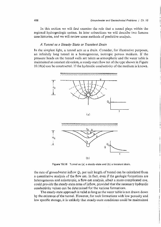
In the simplest light, a tunnel acts as a drain. Consider, for illustrative purposes, an infinitely long tunnel in a homogeneous, isotropic porous medium. If the pressure heads on the tunnel walls are taken as atmospheric and the water table is maintained at constant elevation, a steady-state flow net of the type shown in Figure 10.16(a) can be constructed. If the hydraulic conductivity of the medium is known,

'//II /1717///// 171711111111111117111/7/17////1///11/

T Ho

1

(a)

7//1 ///////II //1//l/111 //1 /////I/// /7/1////1111///l

( b)

Figure 10.16 Tunnel as (a) a steady-state and (b) a transient drain.

the rate of groundwater inflow Q0 per unit length of tunnel can be calculated from a quantitative analysis of the flow net. In fact, even if the geologic formations are heterogeneous and anisotropic, a flow-net analysis, albeit a more complicated one, could provide the steady-state rates of inflow, provided that the necessary hydraulic conductivity values can be determined for the various formations.

The steady-state approach is valid as long as the water table is not drawn down by the existence of the tunnel. However, for rock formations with low porosity and low specific storage, it is unlikely that steady-state conditions could be maintained


for long in the presence of a tunnel. It is more likely [Figure 1O.l6(b )] that a transient flow system will develop with declining water tables above the tunnel. In that case the initial steady-state inflow rate Q 0 per unit length of tunnel will decrease as a function of time.

If geologic conditions were always simple and an infinitely long tunnel could be instantaneously driven, the calculation of tunnel inflows would be a simple matter. Unfortunately, the geology along a tunnel line is seldom as homogeneous as the use of the two-dimensional cross sections of Figure 10.16 would imply. There is usually an alternating sequence of more-permeable and less-permeable formations, and the inflows along a tunnel line are seldom constant through space, let alone time. Very often it is extreme inflows from one small, unexpected, highpermeability zone that leads to the greatest difficulties. Unconsolidated sand and gravel deposits and permeable sedimentary strata such as sandstone or limestone can lead to water problems. More often, it is very localized secondary features such as solution cavities, and fracture zones associated with faults or other structural features, that lead to the largest inflows at the face.

In short, then, tunnelers must be ready to cope with two main types of groundwater inflow: (I) regional inflows along the tunnel line, and (2) catastrophic inflows at the face. The first type can usually be analyzed with a steady-state flow-net analysis. Flows are relatively small and decrease slowly with time. It is usually possible to design for them with tunnel drainage systems. Flows of the second type are very difficult to predict. They may be very large but decrease rapidly with time. It is difficult to design economic drainage systems for them, and they create an especially dangerous hazard if the tunnel is being driven downhill or from a closed heading. Inflows greater than 1000 t /s have been recorded at tunnel headings in several tunnels during their construction (Goodman et al., 1965).

Hydrogeo!ogic Hazards of Tunneling

Large groundwater inflows into tunnels are sometimes associated with high temperatures and noxious gases. The first usually occurs in deep tunnels under the influence of the thermal gradient, or in areas of recent volcanic or seismic activity. Explosive gases such as methane are known to occur in coals and shales, and the coal-mining industry long ago learned to respect their power. In tunneling, however, it is usually difficult to anticipate their occurrence.

At the Tecolate Tunnel (Trefzger, 1966), all the main hazards of tunneling occurred together to create what has become the classic case history in the field. The Tecolate Tunnel was driven through the Santa Ynez mountains 19 km northwest of Santa Barbara, California, during the period 1950-1955. It is 10.3 km long and 2.1 min diameter. It is an aqueduct that carries water from a supply reservoir to the Santa Barbara metropolitan district. The tunnel penetrates a sequence of poorly consolidated shales, siltstones, sandstones, and conglomerates, and crosses one major fault and several minor ones. Major groundwater inflows were encountered with the temperature of the inflows ranging between 11 and 41°C at the face. The largest inflows at the face reached 580 t /s at temperatures up to 40°C. One


inflow at 180 t/s held up construction for 16 months and resisted all grouting attempts. All flows came from intensely fractured siltstones and sandstones. The temperatures are thought to have been caused by residual heat from geologically recent faulting. To cope with the almost unbearable conditions in the tunnel, workmen traveled to and from the heading in mine cars immersed up to their necks in cold water.

The San Jacinto tunnel near Banning, California (Thompson, 1966), is one component of the Colorado River Aqueduct, which delivers water from the Colorado watershed to the Los Angeles area. Preconstruction geologic studies led to the conclusion that the predominant rock type would be massive granite. Although some suggestion of faulting was noted, no one visualized the tremendous volumes of water that were later found to be associated with these structural features.

The tunnel was driven from two headings serviced by a central shaft. With the tunnel advanced only· about 50 m from the shaft, a heavy flow of water, estimated at 480 t/s, surged into the heading accompanied by over 760 m 3 of rock debris. The limited sections of tunnel east and west of the shaft were soon flooded and water ultimately filled the 250 m shaft to within 45 m of the surface.

The source of the water was a fractured fault zone with a particularly malicious configuration. The fault zone was bounded on the footwall side by a thin layer of impermeable clay gouge. The water-bearing zone occurred in the heavily fractured hanging wall. The initial tunnel heading intercepted the fault from the footwall side with the resultant catastrophic inflow. Subsequent mapping located 21 faults along the tunnel line, each with the same internal "stratigraphy" as the original fault. Subsequent tunneling experience showed that the headings that approached the fault zones from the hanging-wall side still encountered large inflows of groundwater, but by intercepting smaller flows sooner, and by spreading the total flow over a larger area and over a longer time, catastrophic inflows were avoided.

Predictive Analysis of Groundwater Inflows Into Tunnels

If tunnelers are to be expected to cope safely and efficiently with large groundwater inflows, hydrogeologists and geotechnical engineers are going to have to develop more reliable methods of predictive analysis. The only theoretical analyses that we could find in the literature for the prediction of groundwater inflows into tunnels are those of Goodman et al. (1965). They represent an excellent initial attack on the problem but are far from the final work. They show that for the case of a tunnel of radius r acting as a steady-state drain [Figure 10.16(a)] in a homogeneous, isotropic media with hydraulic conductivity K, the rate of groundwater inflow Q0

per unit length of tunnel is given by

_ 2nKH0 Qo - 2.3 log (2H0/r)

(10.17)

Their analysis for the transient case [Figure 10.16(b)] shows the rate cumulative of inflow Q ( t) per unit length of tunnel at any time t after the breakdown of steady flow to


be given by

Q(t) = (8f KH~Syf) 112

(10.18)

where K is the hydraulic conductivity of the medium, SY is the specific yield, and C is an arbitrary constant. The development of Eq. (10.18), however, is based on a very restrictive set of assumptions. It assumes that the water table is parabolic in shape and that the Dupuit-Forchheimer horizontal flow assumptions hold. In addition, Eq. (10.18) is only valid for flow conditions that arise after the water-table decline has reached the tunnel, that is, after t3 in Figure 10.16(b). On the basis of Dupuit-Forchheimer theory, the constant C in Eq. (10.18) should be 0.5, but Goodman et al. (1965), on the basis of laboratory modeling studies, found that a more suitable value approached 0.75. Equation (10.18) may be suitable for orderof-magnitude design-inflow estimates, but it should be used with a healthy dose of skepticism.

For more complex hydrogeologic environments that cannot be represented by the idealized configurations of Figure 10.16, numerical mathematical models can be prepared for each specific case. Goodman et al. (1965) provide a transient analysis for the prediction of inflows at the face from a vertical water-bearing zone. Wittke et al. (1972) describe the application of a finite-element model to a tunnel line in jointed rock. Their analysis is based on the discontinuous approach to flow in fractured rock (Section 2.12) rather than the continuous approach followed by Goodman et al. (1965).

We have, in this section, considered only those groundwater problems that arise during construction of a tunnel. If the tunnel is to carry water, and if that water is to be under pressure, there are design considerations that are influenced by the interactions between tunnel flow and groundwater flow during operation. If the tunnel is to be unlined, an analysis must be made of the water losses that will occur to the regional flow system under the influence of the high hydraulic heads that will be induced in the rocks at the tunnel boundary. If the tunnel is to be lined, its design must take into account the pressures that will be exerted on the outside of the lining by the groundwater system when the tunnel is empty.

For these purposes, steady-state and transient flow nets can once again be used to advantage. For a more detailed treatment of the design aspects, the reader is referred to texts on engineering geology or rock mechanics, such as those by Krynine and Judd (1957) or Jaeger (1972).

10.4 Groundwater Inflows Into Excavations

Any engineering excavation that must be taken below the water table will encounter groundwater inflow. The rates of inflow will depend on the size and depth of the excavation and on the hydrogeological properties of the soils or rocks being excavated. At sites where the soil or rock formations have low hydraulic conductivities,


only small inflows will occur, and these can usually be handled easily by pumpage from a sump or collector trench. In such cases a sophisticated hydrogeological analysis is seldom required. In other cases, particularly in silts and sands, dewatering of excavations can become a significant aspect of engineering construction and design.

Drainage systems also serve other purposes, apart from the lowering of water tables and the interception of seepage. They reduce uplift pressures and uplift gradients on the bottom of an excavation, thus providing protection against bottom heave and piping. A dewatered excavation also leads to reduced pore pressures on its slopes so that slope stability is improved. In the design of open pit mines, this is a factor of some importance; if decreased pore pressures can lead to an increase in the design pit-slope of even 1°, the savings created by reduced excavation can be many millions of dollars.

Drainage and Dewatering of Excavations

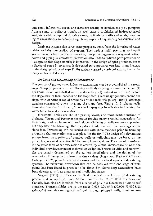
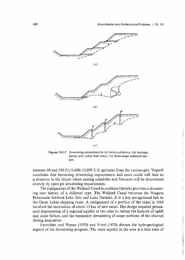
The control of groundwater inflow to excavations can be accomplished in several ways. Sharp (in press) lists the following methods as being in current wide use: (1) horizontal drainholes drilled into the slope face; (2) vertical wells drilled behind the slope crest or from benches on the slope face; (3) drainage galleries behind the slope, with or without radial drainholes drilled from the gallery; and ( 4) drainage trenches constructed down or along the slope face. Figure 10.17 schematically illustrates how the first three of these techniques can be effective in lowering the water table around an excavation.

Horizontal drains are the cheapest, quickest, and most flexible method of drainage. Piteau and Peckover (in press) provide many practical suggestions for their design and emplacement in rock slopes. Galleries or wells are more expensive, but they have the advantage that they do not inferfere with the workings on the slope face. Dewatering can be carried out with these methods prior to breaking ground so that excavation can take place "in the dry." The design of a dewatering system based on a pattern of pumped wells or wellpoints must be based on the principles presented in Section 8.3 for multiple well systems. The cone of drawdown in the water table at the excavation is created by mutual interference between the individual drawdown cones of each well or wellpoint. Transmissivities and storativities are usually determined on the earliest installations and the design of the remainder of the system is based on these values. Briggs and Fiedler (1966) and Cedergren (1975) provide detailed discussions of the practical aspects of dewatering systems. The maximum drawdown that can be achieved with one stage of wellpoints has been found in practice to be about 5 m. Some deep excavations have been dewatered with as many as eight wellpoint stages.

V ogwill ( 197 6) provides an excellent practical case history of dewatering problems at an open pit mine. At Pine Point in the North West Territories of Canada, lead-zinc ore is mined from a series of pits in a Devonian dolomite reef complex. Transmissivities are in the range 0.005-0.01 m2/s (30,000-70,000 U.S. gal/day/ft) and dewatering, carried out through pumped wells, must remove

493

(a)

Groundwater and Geotechnica/ Problems / Ch. 10

-/

\~----~---~ (b)

( c)

Figure 10.17 Dewatering excavations by (a) horizontal drains; (b) drainage gallery with radial drain holes; (c) three-stage wellpoint system.

between 60 and 950 t/s (1,000-15,000 U.S. gal/min) from the various pits. Vogwill concludes that increasing dewatering requirements and costs could well lead to a situation in the future where mining schedules and forecasts will be determined entirely by open pit dewatering requirements.

The realignment of the Welland Canal in southern Ontario provides a dewatering case history of a different type. The Welland Canal traverses the Niagara Penninsula between Lake Erie and Lake Ontario. It is a key navigational link in the Great Lakes shipping route. A realignment of a portion of the canal in 1968 involved the excavation of about 13 km of new canal. The design required permanent depressuring of a regional aquifer at two sites to reduce the hazards of uplift and slope failure, and the temporary dewatering of some portions of the channel during excavation.

Farvolden and Nunan (1970) and Frind (1970) discuss the hydrogeological aspects of the dewatering program. The main aquifer in the area is a thin zone of


fractured dolomite found on the bedrock surface immediately below 20-30 m of low-permeability, unconsolidated glacial and lacustrine deposics. Extensive drilling and sampling was carried out along the axis of the new channel, and piezometers were installed at various locations in both the surficial deposits and the bedrock. Pumping tests run in the dolomite aquifer to determine aquifer coefficients, showed that transmissivities varied widely, but values as high as 0.015 m2/s (90,000 IGPD/ ft) were not uncommon. These high transmissivities had both positive and negative implications for the project. On the positive side, they made it possible to dewater the entire construction site from just four pumping centers. On the negative side, they led to extensive areal propagation of the drawdown cones in an aquifer that is widely exploited by private, municipal, and industrial wells. A numerical aquifer simulation was carried out for predictive purposes, and one of its primary goals was the determination of responsibility for drawdowns in areas of mutual interference. Results of the simulation showed that pumping rates of about 100 f, /s would provide the necessary 10 m drawdown along the realignment route. The simulation also showed that an elliptical cone of drawdown would affect water levels as far as 12 km from the canal.

Predictive Analysis of Groundwater Inflows Into Excavations

The development of quantitative methods of analysis for the prediction of groundwater inflow into excavations has lagged behind the development of such methods for many other problems in applied groundwater hydrology. The only analytical methods known to the authors are adaptations of methods designed for the prediction of inflow hydrographs to surface reservoirs from large unconfined aquifers. Brutsaert and his coworkers have analyzed the problem first presented in Figure 5.14 using each of the approaches schematically illustrated there. Verma and Brutsaert (1970) solved the complete saturated-unsaturated system with a numerical method. Verma and Brutsaert (1971) solved the problem numerically as a twodimensional, saturated, free-surface problem; and analytically as a one-dimensional, saturated problem simplified by use of the Dupuit assumptions. The predictive methodology of Figure 10.18 is based on an earlier study (Ibrahim and Brutsaert, 1965) carried out with a laboratory model. The results were later confirmed by the mathematical models of Verma and Brutsaert (1970, 1971).

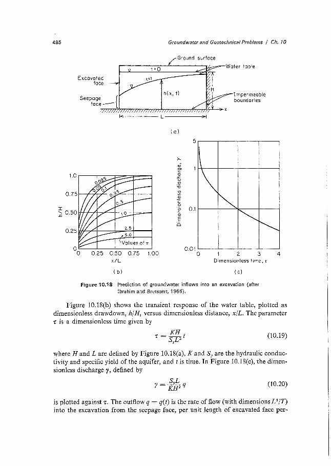
Figure 10.18(a) shows the geometry of the two-dimensional vertical cross section under analysis. It has relevance to the prediction of groundwater inflows into excavations only if the following assumptions and limitations are noted: (1) the excavated face is vertical; (2) the excavation is em placed instantaneously; (3) the boundary conditions and initial conditions on the hydrogeological system are as shown on Figure 10.18(a); (4) the geological stratum is homogeneous and isotropic; and (5) the excavation is long and lineal iri shape, rather than circular, so that the two-dimensional cartesian symmetry is applicable. While these assumptions may appear restrictive, results may nevertheless be of use in estimating the probable transient response of more complex systems.

495

I

Groundwater and Geotechnical Problems I Ch. 10

(al

>-...

al 2' 0

..c: u <fl

:.0 <fl <fl Q)

c: 0 ·v;

5

Impermeable boundaries

' 0.50 ........... _........._ ____ ,__ 0.1 c: Q) ..c: E

0

0.01 .__ _ ___._ __ _..___ __ _._ _ ___, 0.25 0.50 0.75 1.00

x/L

(bl

0 2 3 Dimensionless time, r

( C)

Figure 10.18 Prediction of groundwater inflows into an excavation (after Ibrahim and Brutsaert, 1965).

4

Figure 1O.l8(b) shows the transient response of the water table, plotted as dimensionless drawdown, hf H, versus dimensionless distance, x/L. The parameter -c is a dimensionless time given by

KH 'C = s L2 t (10.19)

y

where Hand Lare defined by Figure 10.18(a), Kand Sy are the hydraulic conductivity and specific yield of the aquifer, and tis time. In Figure 10.18(c), the dimensionless discharge y, defined by

(10.20)

is plotted against -c. The outflow q = q( t) is the rate of flow (with dimensions L3 /T) into the excavation from the seepage face, per unit length of excavated face per-


pendicular to the plane of the diagram in Figure 10.IS(a). To apply the method to a specific case, one must know K, Sy, H, and L. 7: is calculated from Eq. (10.19) and h(x, t) is determined from Figure 10.18(b). The y(T) values determined from Figure 10.18(c) can be converted to q(t) values through Eq. (10.20). The formulas and graphs can be used with any set of consistent units.

It is possible to carry out similar analyses for circular pits, and for cases where the external boundary is a constant-head boundary, with h(L, t) = Hfor all t > 0, rather than an impermeable boundary.

Suggested Readings

CASAGRANDE, A. 1961. Control of seepage through foundations and abutments of dams. Geotechnique, 11, pp. 161-181.

GOODMAN, R. E., D. G. MOYE, A. VAN SCHALKWYK, and I. JAVANDEL. 1965. Ground water inflows during tunnel driving. Eng. Geo!., pp. 39-56.

JAEGER, J.C. 1971. Friction of rocks and stability of rock slopes. Geotechnique, 21, pp. 97-134.

TERZAGHI, K. 1950. Mechanism of landslides. Berkey Volume: Application of Geology to Engineering Practice. Geological Society America, New York, pp. 83-123.

10.1 pore pressures, landslides, - hwbhydrogeologistswithoutborders.org/wordpress/wp... · 10.1...

Documents