1 np-complete problems polynomial time vs exponential time –polynomial o(n k ), –where n is the...
TRANSCRIPT
1
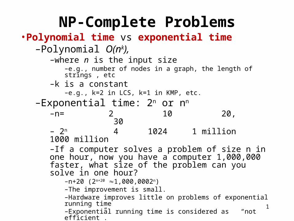
NP-Complete Problems•Polynomial time vs exponential time
–Polynomial O(nk), –where n is the input size
–e.g., number of nodes in a graph, the length of strings , etc –k is a constant
–e.g., k=2 in LCS, k=1 in KMP, etc.
–Exponential time: 2n or nn
–n= 2 10 20, 30 – 2n 4 1024 1 million 1000 million–If a computer solves a problem of size n in one hour, now you have a computer 1,000,000 faster, what size of the problem can you solve in one hour?
–n+20 (2n+20 1,000,0002n)–The improvement is small.–Hardware improves little on problems of exponential running time–Exponential running time is considered as “not efficient”.
2
Story
• All algorithms we have studied so far are polynomial time algorithms (unless specified).• Facts: people have not yet found any polynomial time algorithms for some famous problems, (e.g., Hamilton Circuit, longest simple path, Steiner trees).• Question: Do there exist polynomial time algorithms for those famous problems?• Answer: No body knows.
3
Story•Research topic: Prove that polynomial time algorithms do not exist for those famous problems, e.g., Hamilton circuit problem.
•Turing award
•Vinay Deolalikar attempted 2010, but failed.
•An article on The New Yorker http://www.newyorker.com/online/blogs/elements/2013/05/a-most-profound-math-problem.html
•To answer the question, people define two classes•P class
•NP class.
•To answer if PNP, a rich area, NP-completeness theory is developed.
4
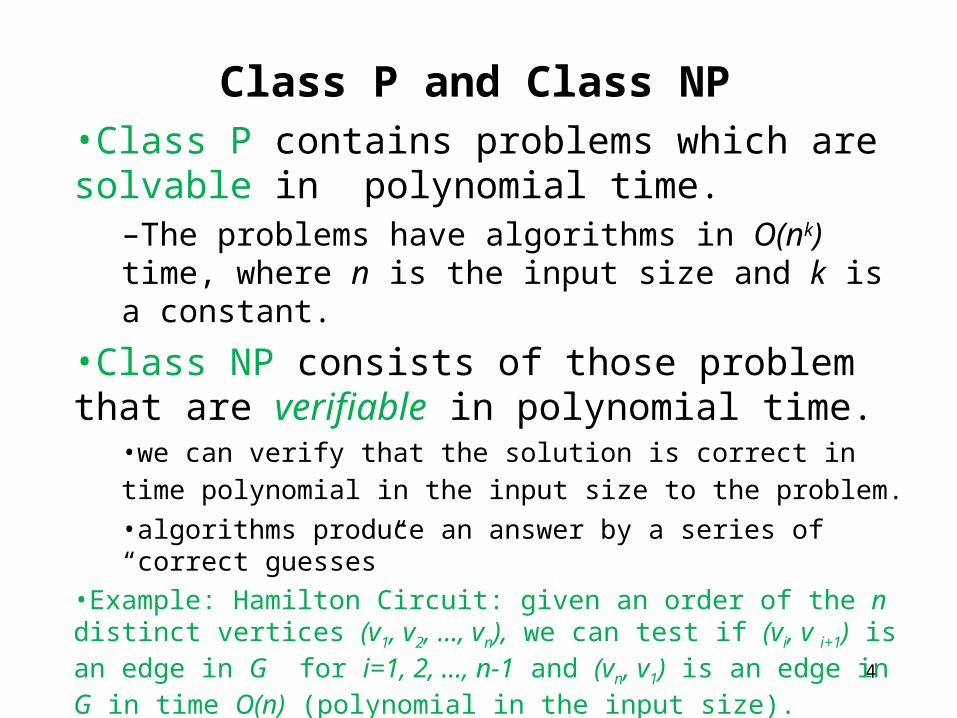
Class P and Class NP•Class P contains problems which are solvable in polynomial time.
–The problems have algorithms in O(nk) time, where n is the input size and k is a constant.
•Class NP consists of those problem that are verifiable in polynomial time.
•we can verify that the solution is correct in time polynomial in the input
size to the problem. •algorithms produce an answer by a series of “correct guesses”
•Example: Hamilton Circuit: given an order of the n distinct vertices (v1, v2, …, vn), we can test if (vi, v i+1) is an edge in G for i=1, 2, …, n-1 and (vn, v1) is an edge in G in time O(n) (polynomial in the input size).
5
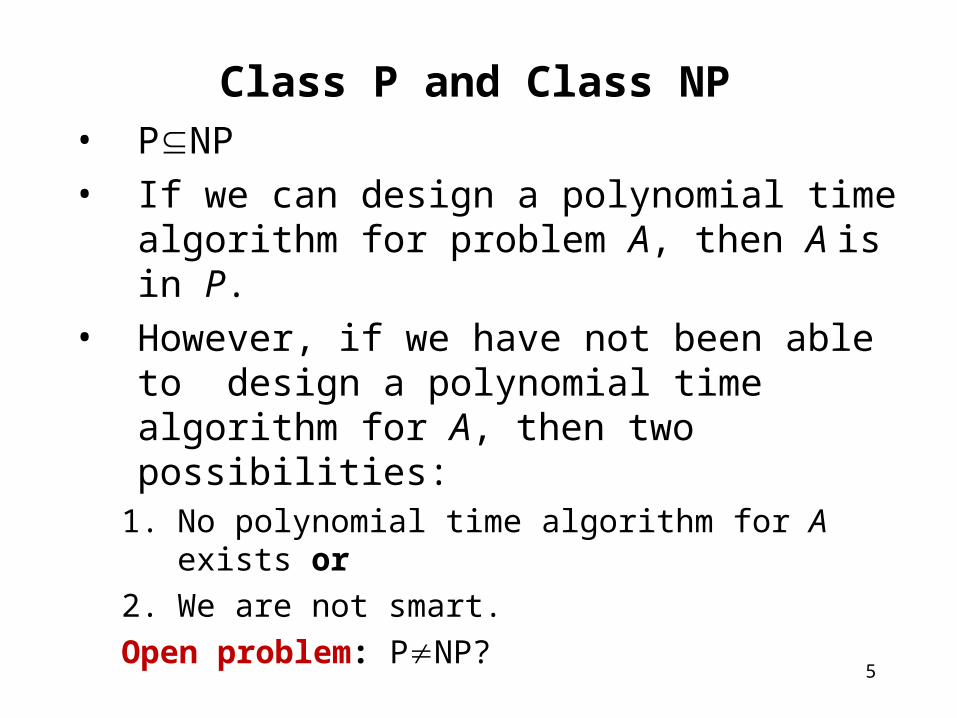
Class P and Class NP• PNP• If we can design a polynomial time algorithm for
problem A, then A is in P.• However, if we have not been able to design a
polynomial time algorithm for A, then two possibilities:
1. No polynomial time algorithm for A exists or
2. We are not smart.
Open problem: PNP?
6
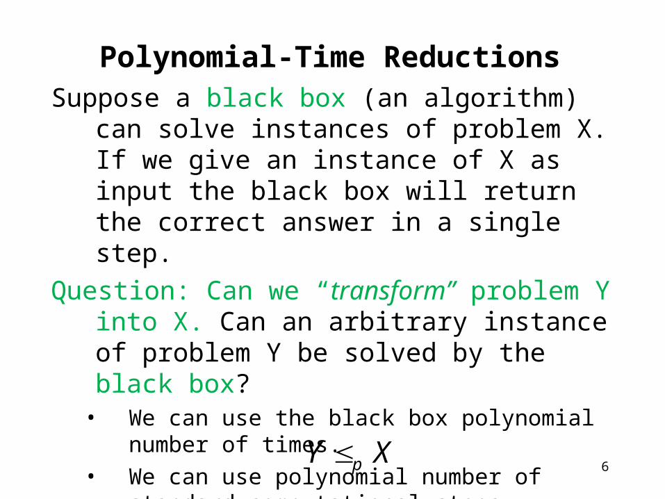
Polynomial-Time ReductionsSuppose a black box (an algorithm) can solve instances
of problem X. If we give an instance of X as input the black box will return the correct answer in a single step.
Question: Can we “transform” problem Y into X. Can an arbitrary instance of problem Y be solved by the black box?• We can use the black box polynomial number of times.
• We can use polynomial number of standard computational steps
• If yes, then Y is polynomial-time reducible to X.
XY p
7
NP-Complete• A problem X is NP-complete if
• it is in NP, and
•any problem Y in NP has a polynomial time reduction to X.
•it is the hardest problem in NP.
•If ONE NP-complete problem can be solved in polynomial time, then any problem in class NP can be solved in polynomial time.
•The first NPC problem is Satisfiability problem –Proved by Cook in 1971 and obtains the Turing Award for this work
8
Boolean formula• A boolean formula f(x1, x2, …xn), where xi are boolean variables (either 0 or 1), contains boolean variables and boolean operations AND, OR and NOT . • Clause: variables and their negations are connected with OR operation, e.g., (x1 OR NOTx2 OR x5)
• Conjunctive normal form of boolean formula:
contains m clauses connected with AND operation.
Example:
(x1 OR NOT x2) AND (x1 OR NOT x3 OR x6) AND (x2 OR x6) AND (NOT x3 OR x5).
–Here we have four clauses.
9
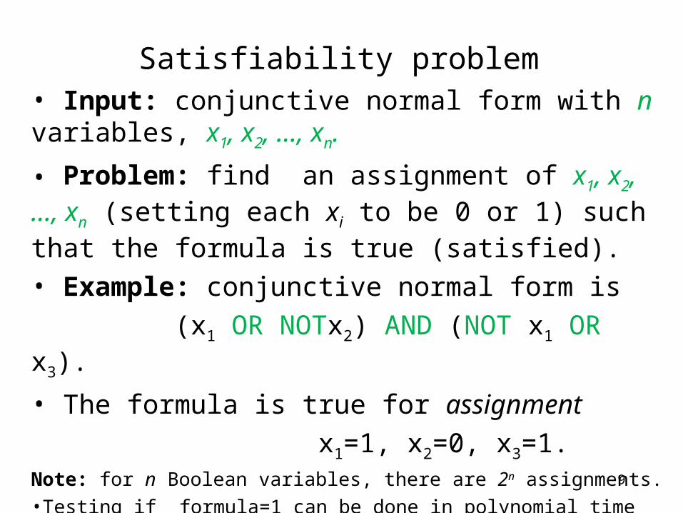
Satisfiability problem• Input: conjunctive normal form with n variables, x1, x2, …, xn.
• Problem: find an assignment of x1, x2, …, xn (setting each xi to be 0 or 1) such that the formula is true (satisfied).
• Example: conjunctive normal form is
(x1 OR NOTx2) AND (NOT x1 OR x3).
• The formula is true for assignment
x1=1, x2=0, x3=1. Note: for n Boolean variables, there are 2n assignments.
•Testing if formula=1 can be done in polynomial time for any given assignment.
•Given an assignment that satisfies formula=1 is hard.
10
The First NP-complete Problem• Theorem: Satisfiability problem is NP-complete.
–It is the first NP-complete problem.–Stephen. A. Cook in 1971 http://en.wikipedia.org/wiki/Stephen_Cook
–Won Turing prize for his work.
• Significance:–If Satisfiability problem is in P, then ALL problems in class NP are in P.
–To solve PNP, you should work on NPC problems such as satisfiability problem.
–We can use the first NPC problem, Satisfiability problem, to show other NP-complete problems.
11
How to show that a problem is NPC?•To show that problem A is NP-complete, we can
–First, find a NP-complete problem B.–Then, show that
–IF problem A is P, then B is in P.–that is, to give a polynomial time reduction from B to A.
Remarks: Since a NPC problem, problem B, is the hardest in class NP, problem A is also the hardest
12
Hamilton circuit and Longest Simple Path • Hamilton circuit : a circuit uses every vertex
of the graph exactly once except for the last vertex, which duplicates the first vertex.
– It was shown to be NP-complete. • Longest Simple Path:
– Input: V={v1, v2, ..., vn} be a set of nodes in a graph G and d(vi, vj) the distance between vi and vj,,
– Output: a longest simple path from u to v .
• Theorem 2: The longest simple path problem is NP-complete.
13
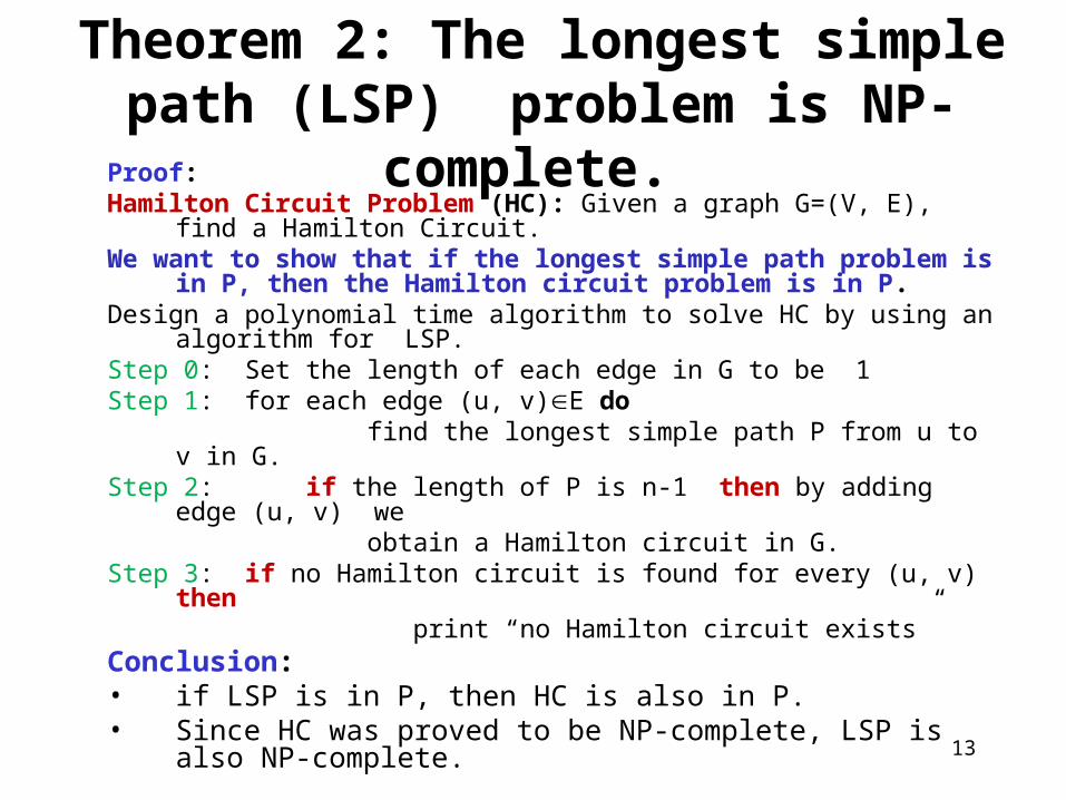
Theorem 2: The longest simple path (LSP) problem is NP-complete.
Proof: Hamilton Circuit Problem (HC): Given a graph G=(V, E), find a Hamilton
Circuit.We want to show that if the longest simple path problem is in P, then the
Hamilton circuit problem is in P. Design a polynomial time algorithm to solve HC by using an algorithm for LSP. Step 0: Set the length of each edge in G to be 1Step 1: for each edge (u, v)E do find the longest simple path P from u to v in G.Step 2: if the length of P is n-1 then by adding edge (u, v) we obtain a Hamilton circuit in G.Step 3: if no Hamilton circuit is found for every (u, v) then print “no Hamilton circuit exists”Conclusion: • if LSP is in P, then HC is also in P.• Since HC was proved to be NP-complete, LSP is also NP-complete.
14
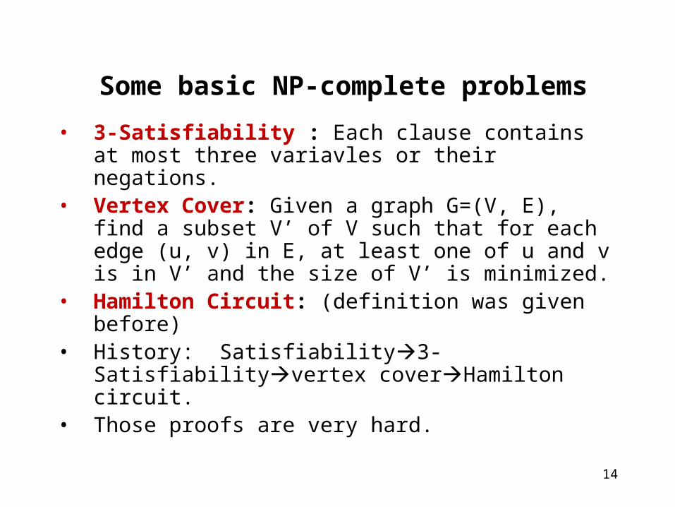
Some basic NP-complete problems
• 3-Satisfiability : Each clause contains at most three variavles or their negations.
• Vertex Cover: Given a graph G=(V, E), find a subset V’ of V such that for each edge (u, v) in E, at least one of u and v is in V’ and the size of V’ is minimized.
• Hamilton Circuit: (definition was given before)
• History: Satisfiability3-Satisfiabilityvertex coverHamilton circuit.
• Those proofs are very hard.
15
Approximation Algorithms •Concepts
•Knapsack
•Steiner Minimum Tree
•TSP
•Vertex Cover
16
Concepts of Approximation Algorithms
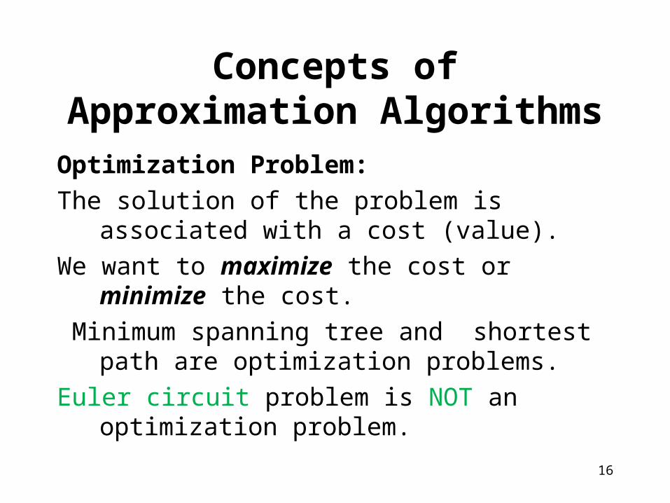
Optimization Problem:
The solution of the problem is associated with a cost (value).
We want to maximize the cost or minimize the cost.
Minimum spanning tree and shortest path are optimization problems.
Euler circuit problem is NOT an optimization problem.
17
Approximation Algorithm
An algorithm A is an approximation algorithm
• if given any instance I, it finds a candidate solution s(I)
How good an approximation algorithm is?
We use performance ratio to measure the quality of an approximation algorithm.
18
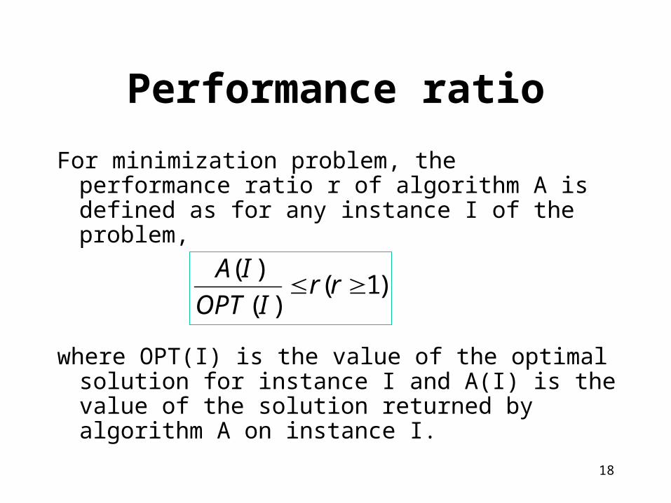
Performance ratio
For minimization problem, the performance ratio r of algorithm A is defined as for any instance I of the problem,
where OPT(I) is the value of the optimal solution for instance I and A(I) is the value of the solution returned by algorithm A on instance I.
)1()(
)( rr
IOPT
IA
19
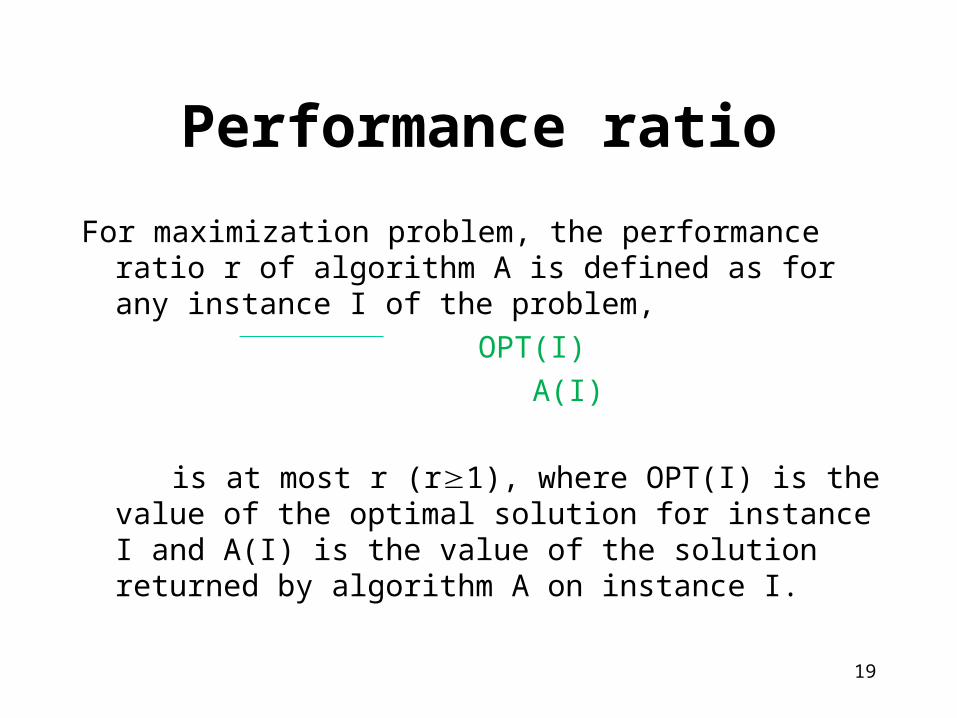
Performance ratio
For maximization problem, the performance ratio r of algorithm A is defined as for any instance I of the problem,
OPT(I)
A(I)
is at most r (r1), where OPT(I) is the value of the optimal solution for instance I and A(I) is the value of the solution returned by algorithm A on instance I.
20
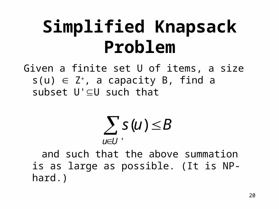
Simplified Knapsack Problem
Given a finite set U of items, a size s(u) Z+, a capacity B, find a subset U'U such that
and such that the above summation is as large as possible. (It is NP-hard.)
'
)(Uu
Bus
21
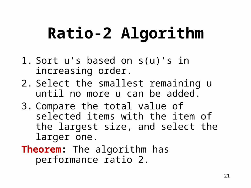
Ratio-2 Algorithm
1. Sort u's based on s(u)'s in increasing order.2. Select the smallest remaining u until no
more u can be added.3. Compare the total value of selected items
with the item of the largest size, and select the larger one.
Theorem: The algorithm has performance ratio 2.
22
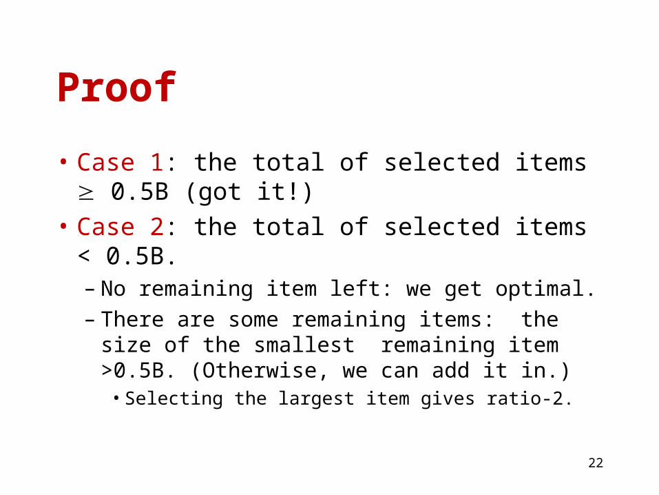
Proof
• Case 1: the total of selected items 0.5B (got it!)
• Case 2: the total of selected items < 0.5B.– No remaining item left: we get optimal.– There are some remaining items: the size of the
smallest remaining item >0.5B. (Otherwise, we can add it in.)
• Selecting the largest item gives ratio-2.
23
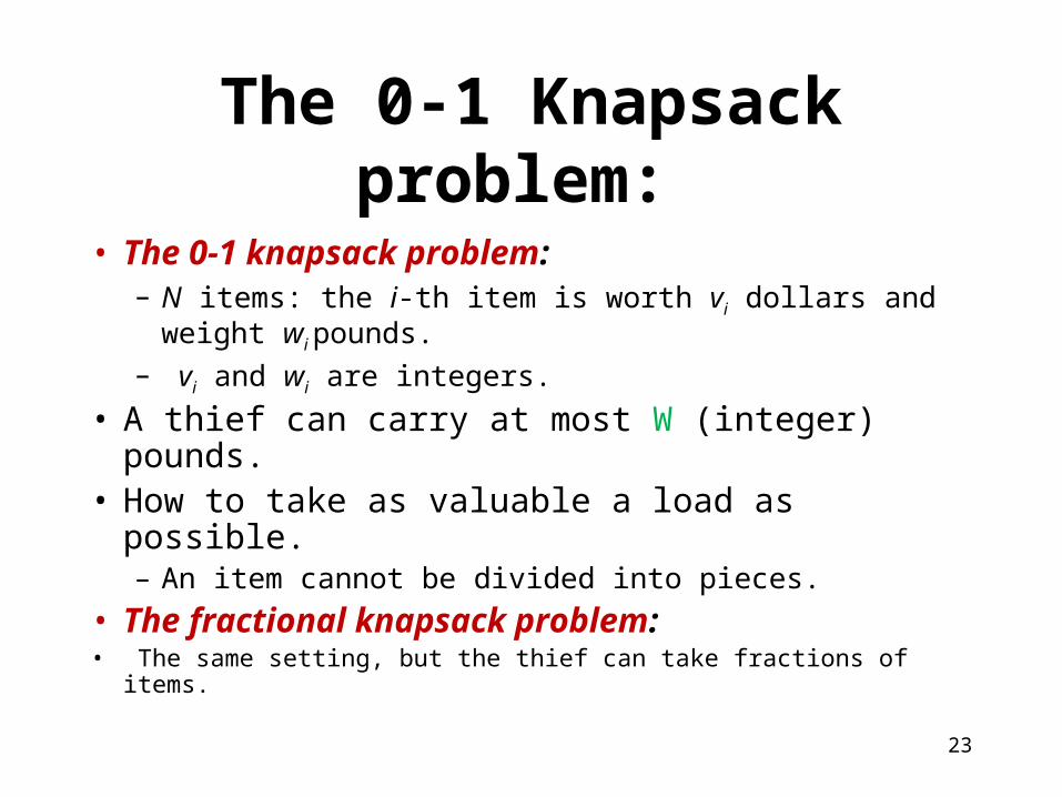
The 0-1 Knapsack problem:
• The 0-1 knapsack problem:– N items: the i-th item is worth vi dollars and weight wi
pounds.– vi and wi are integers.
• A thief can carry at most W (integer) pounds.• How to take as valuable a load as possible.
– An item cannot be divided into pieces.
• The fractional knapsack problem:• The same setting, but the thief can take fractions of items.
24
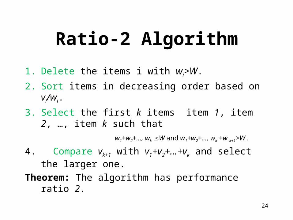
Ratio-2 Algorithm
1. Delete the items i with wi>W.
2. Sort items in decreasing order based on vi/wi.
3. Select the first k items item 1, item 2, …, item k such that
w1+w2+…, wk W and w1+w2+…, wk +w k+1>W.
4. Compare vk+1 with v1+v2+…+vk and select the larger one.
Theorem: The algorithm has performance ratio 2.
25
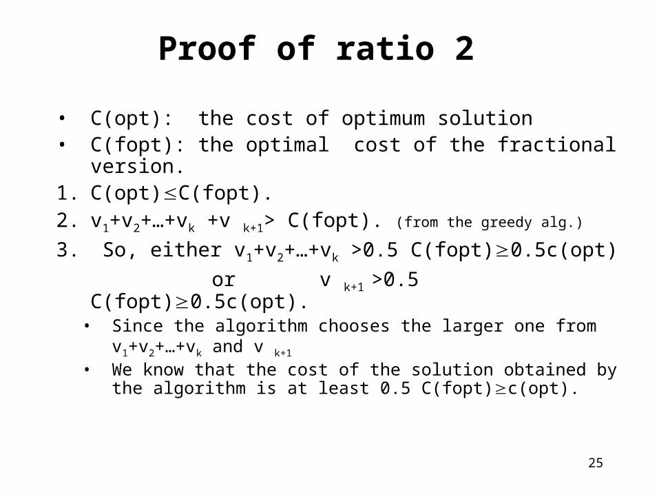
Proof of ratio 2
• C(opt): the cost of optimum solution• C(fopt): the optimal cost of the fractional version.1. C(opt)C(fopt). 2. v1+v2+…+vk +v k+1> C(fopt). (from the greedy alg.)
3. So, either v1+v2+…+vk >0.5 C(fopt)0.5c(opt)
or v k+1 >0.5 C(fopt)0.5c(opt).• Since the algorithm chooses the larger one from v1+v2+
…+vk and v k+1
• We know that the cost of the solution obtained by the algorithm is at least 0.5 C(fopt)c(opt).
26
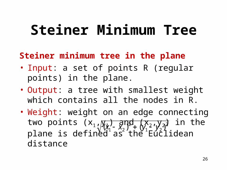
Steiner Minimum Tree
Steiner minimum tree in the plane• Input: a set of points R (regular points) in the plane.• Output: a tree with smallest weight which contains
all the nodes in R.• Weight: weight on an edge connecting two points
(x1,y1) and (x2,y2) in the plane is defined as the Euclidean distance 2
212
21 )()( yyxx
27
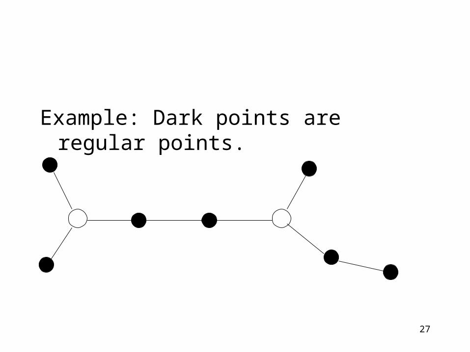
Example: Dark points are regular points.
28
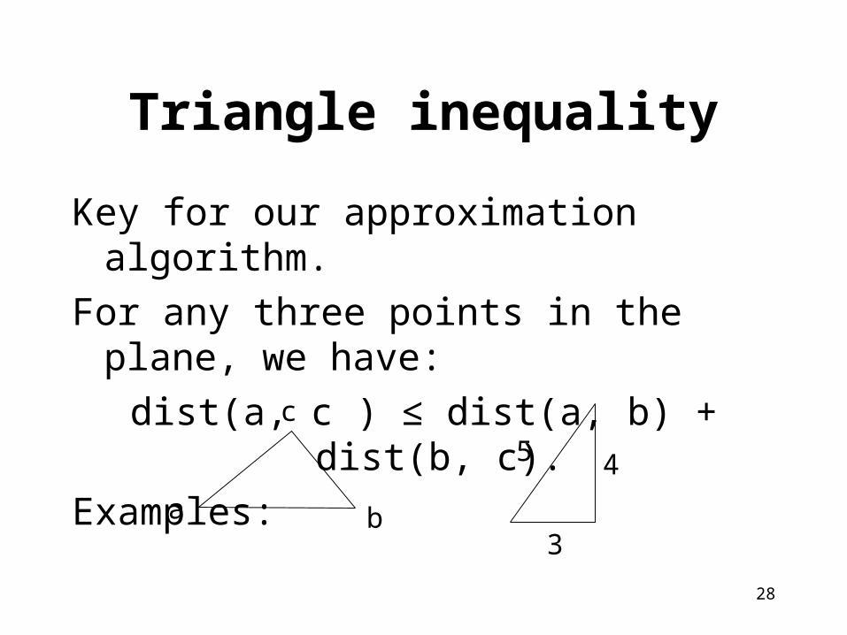
Triangle inequality
Key for our approximation algorithm.
For any three points in the plane, we have:
dist(a, c ) ≤ dist(a, b) + dist(b, c).
Examples:
a b
c
3
45
29
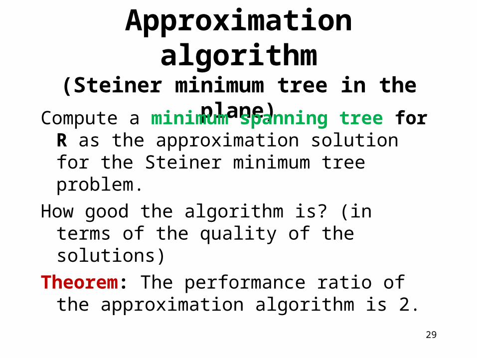
Approximation algorithm(Steiner minimum tree in the plane)
Compute a minimum spanning tree for R as the approximation solution for the Steiner minimum tree problem.
How good the algorithm is? (in terms of the quality of the solutions)
Theorem: The performance ratio of the approximation algorithm is 2.
30
We want to show that for any instance (input) I, A(I)/OPT(I) ≤ r (r≥1)
• A(I) is the cost of the solution obtained from our spanning tree algorithm, and
• OPT(I) is the cost of an optimal solution.
Proof
31
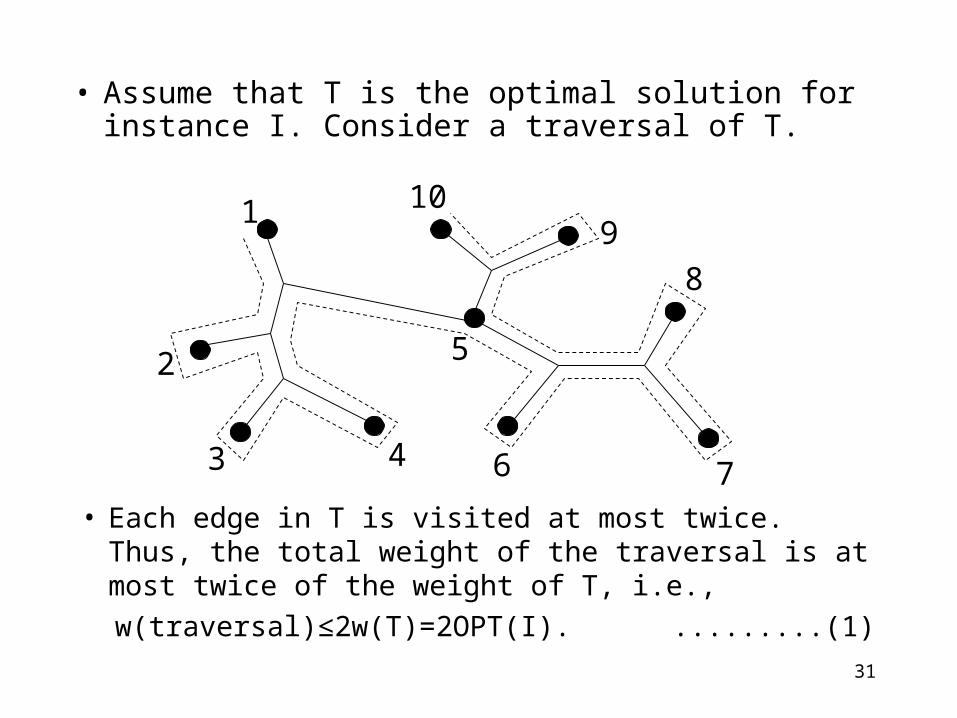
• Assume that T is the optimal solution for instance I. Consider a traversal of T.
1
2
3 4
5
6 7
8
910
• Each edge in T is visited at most twice. Thus, the total weight of the traversal is at most twice of the weight of T, i.e.,
w(traversal)≤2w(T)=2OPT(I). .........(1)
32
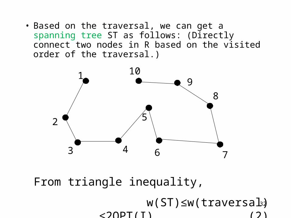
• Based on the traversal, we can get a spanning tree ST as follows: (Directly connect two nodes in R based on the visited order of the traversal.)
7
1
2
3 4
5
6
8
910
From triangle inequality,
w(ST)≤w(traversal) ≤2OPT(I). ..........(2)
33
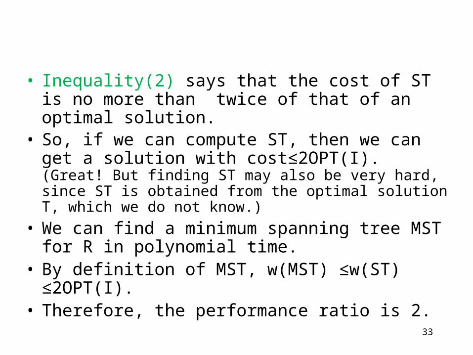
• Inequality(2) says that the cost of ST is no more than twice of that of an optimal solution.
• So, if we can compute ST, then we can get a solution with cost≤2OPT(I).(Great! But finding ST may also be very hard, since ST is obtained from the optimal solution T, which we do not know.)
• We can find a minimum spanning tree MST for R in polynomial time.
• By definition of MST, w(MST) ≤w(ST) ≤2OPT(I).• Therefore, the performance ratio is 2.
34
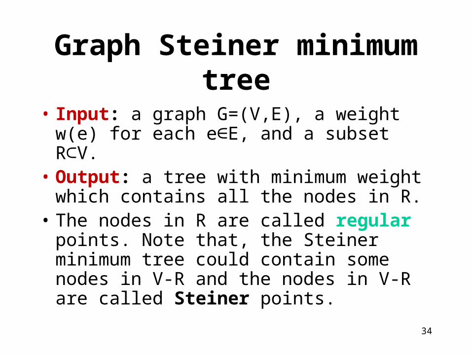
Graph Steiner minimum tree
• Input: a graph G=(V,E), a weight w(e) for each e E, and a subset R∈ V.⊂
• Output: a tree with minimum weight which contains all the nodes in R.
• The nodes in R are called regular points. Note that, the Steiner minimum tree could contain some nodes in V-R and the nodes in V-R are called Steiner points.
35
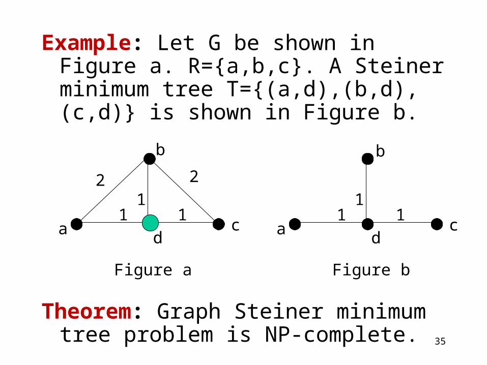
Example: Let G be shown in Figure a. R={a,b,c}. A Steiner minimum tree T={(a,d),(b,d),(c,d)} is shown in Figure b.
Theorem: Graph Steiner minimum tree problem is NP-complete.
b
ad
c1 1
12 2
Figure a
ad
c1 1
1
Figure b
b
36
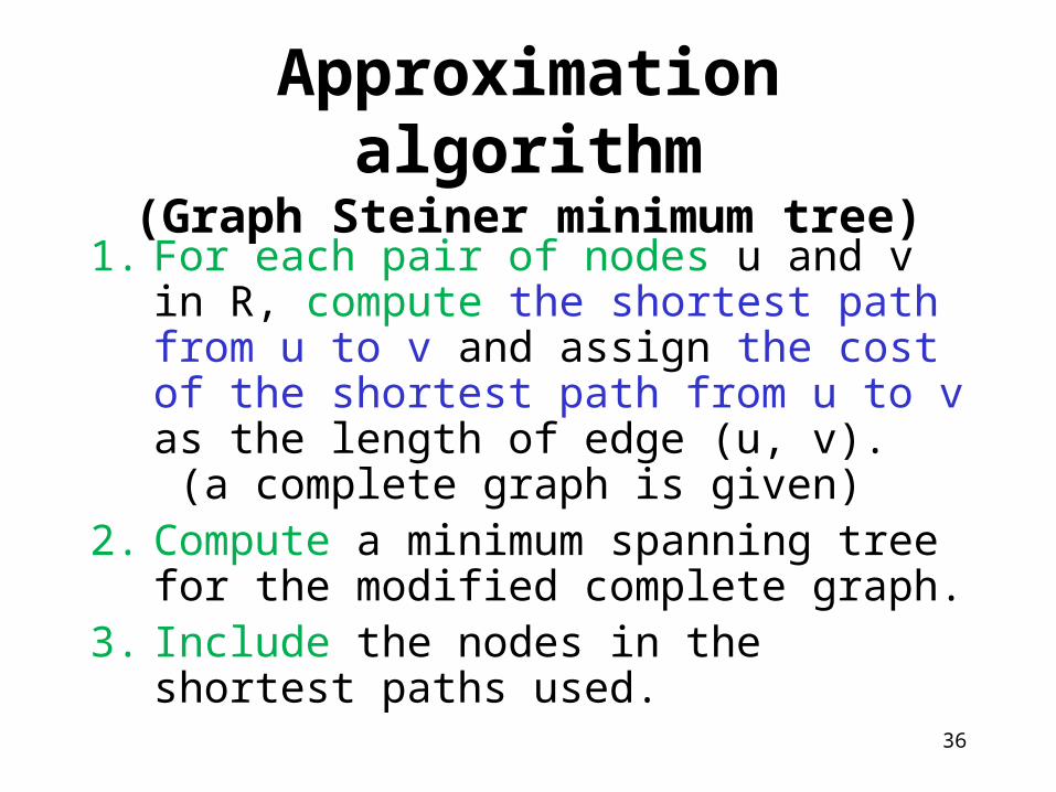
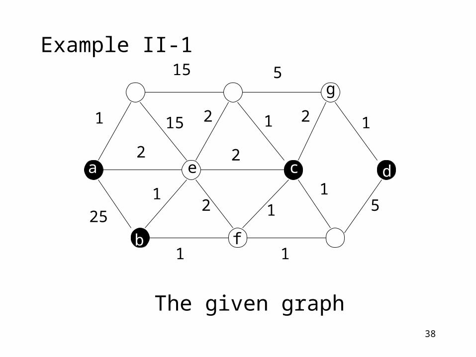
Approximation algorithm(Graph Steiner minimum tree)
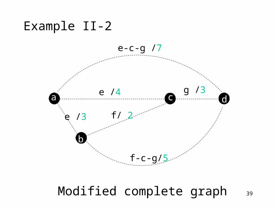
1. For each pair of nodes u and v in R, compute the shortest path from u to v and assign the cost of the shortest path from u to v as the length of edge (u, v). (a complete graph is given)
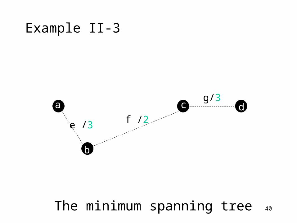
2. Compute a minimum spanning tree for the modified complete graph.
3. Include the nodes in the shortest paths used.
37
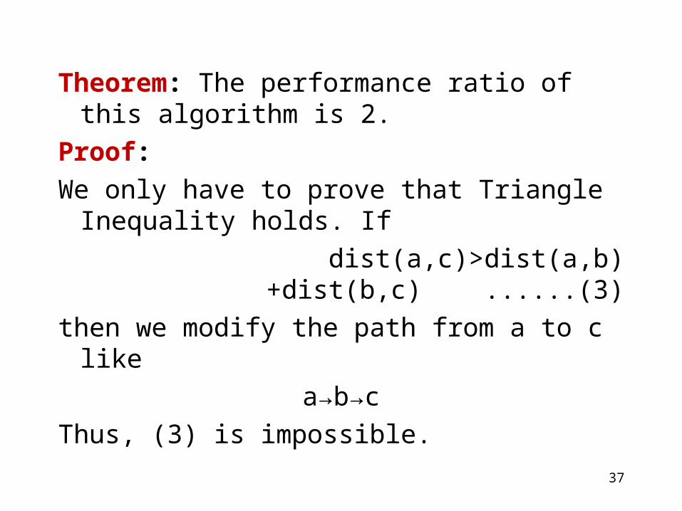
Theorem: The performance ratio of this algorithm is 2.
Proof:
We only have to prove that Triangle Inequality holds. If
dist(a,c)>dist(a,b)+dist(b,c) ......(3)
then we modify the path from a to c like
a→b→c
Thus, (3) is impossible.
38
Example II-1
1
25
15 5
1
5
11
15
2
12
2
2 1 2
11
The given graph
a
b
e c
f
g
d
39
Example II-2
Modified complete graph
a
b
c d
e /3
e /4
f/ 2
g /3
f-c-g/5
e-c-g /7
40
Example II-3
The minimum spanning tree
a
b
c d
e /3 f /2
g/3
41
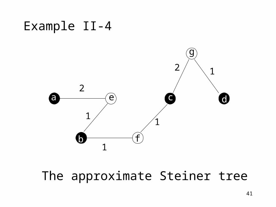
Example II-4
1
1
2
2
1
The approximate Steiner tree
a
b
e c
f
g
d
1
42
Approximation Algorithm for TSP with triangle inequality
• Given n points in a plane, find a tour to visit each city exactly once.
• Assumption: the triangle inequality holds. – that is, d (a, c) ≤ d (a, b) + d (b, c).
• This condition is reasonable, for example, whenever the cities are points in the plane and the distance between two points is the Euclidean distance.
• Theorem: TSP with triangle inequality is also NP-hard.
43
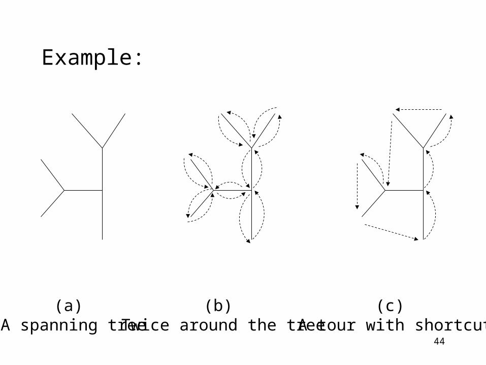
Ratio 2 Algorithm
Algorithm A:1. Compute a minimum spanning tree
algorithm (Figure a)2. Visit all the cities by traversing twice
around the tree. This visits some cities more than once. (Figure b)
3. Shortcut the tour by going directly to the next unvisited city. (Figure c)
44
Example:
(a) A spanning tree
(b) Twice around the tree
(c) A tour with shortcut
45
Proof of Ratio 2
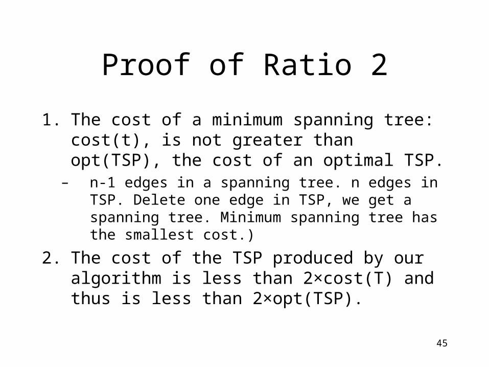
1. The cost of a minimum spanning tree: cost(t), is not greater than opt(TSP), the cost of an optimal TSP.
– n-1 edges in a spanning tree. n edges in TSP. Delete one edge in TSP, we get a spanning tree. Minimum spanning tree has the smallest cost.)
2. The cost of the TSP produced by our algorithm is less than 2×cost(T) and thus is less than 2×opt(TSP).
46
Center Selection Problem
Problem: Given a set of points V in the plane (or some other metric space), find k points c1, c2, .., ck such that for each v in V,
min { i=1, 2, …, k} d(v, ci) d
and d is minimized.
47
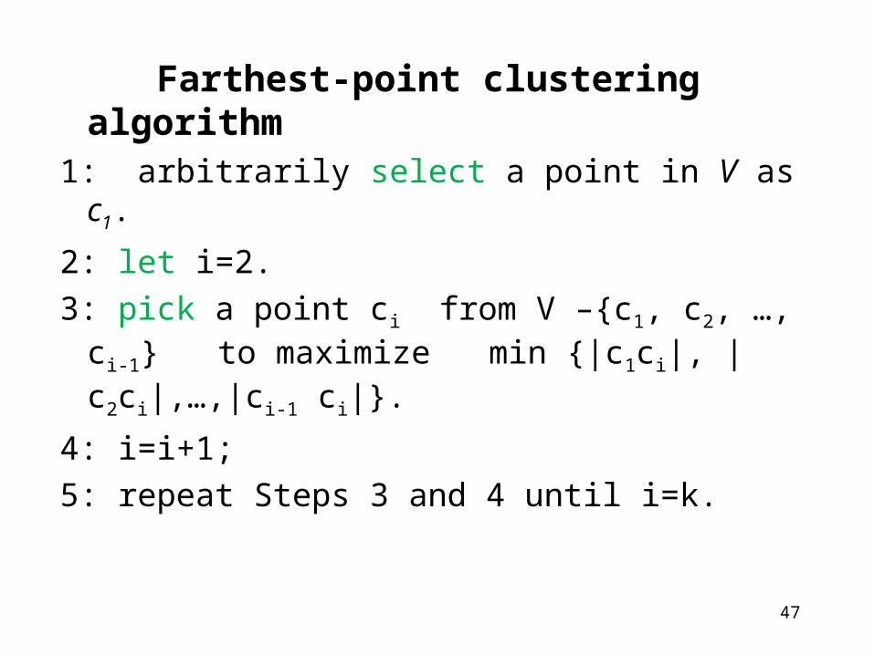
Farthest-point clustering algorithm1: arbitrarily select a point in V as c1.
2: let i=2.
3: pick a point ci from V –{c1, c2, …, ci-1} to maximize min {|c1ci|, |c2ci|,…,|ci-1 ci|}.
4: i=i+1;
5: repeat Steps 3 and 4 until i=k.
48
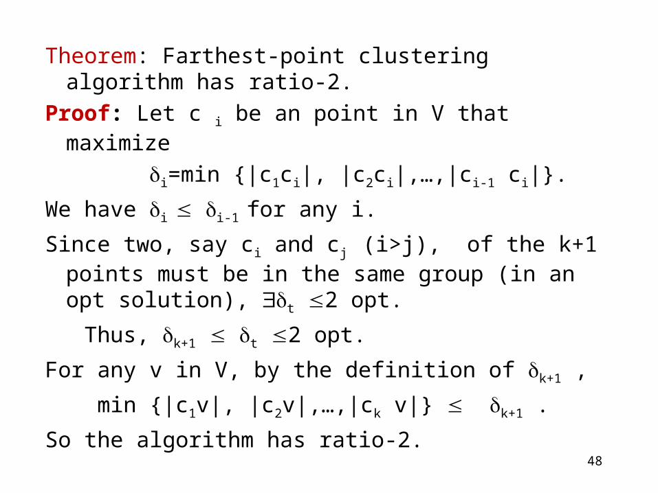
Theorem: Farthest-point clustering algorithm has ratio-2.
Proof: Let c i be an point in V that maximize
i=min {|c1ci|, |c2ci|,…,|ci-1 ci|}.
We have i i-1 for any i.
Since two, say ci and cj (i>j), of the k+1 points must be in the same group (in an opt solution), t 2 opt.
Thus, k+1 t 2 opt.
For any v in V, by the definition of k+1 ,
min {|c1v|, |c2v|,…,|ck v|} k+1 .
So the algorithm has ratio-2.
49
Vertex Cover Problem
• Given a graph G=(V, E), find V'⊆V with minimum number of vertices such that for each edge (u, v)∈E at least one of u and v is in V’.
• V' is called vertex cover.• The problem is NP-hard.• A ratio-2 algorithm exists for vertex cover
problem.