1

MODULE 12

RANDOM VIBRATION

2

Random vibrations are non-periodic. Knowledge of the past history of random vibration is

adequate to predict the probability of occurrence of acceleration, velocity and displacement

magnitudes, but it is not sufficient to predict the precise magnitude at a specific instant.

For most structural vibrations the excitation such as force or base acceleration alternates evenly

about zero. Consequently, mean values characterizing the excitation as well as responses to that

excitation such as displacement or stress are equal to zero.

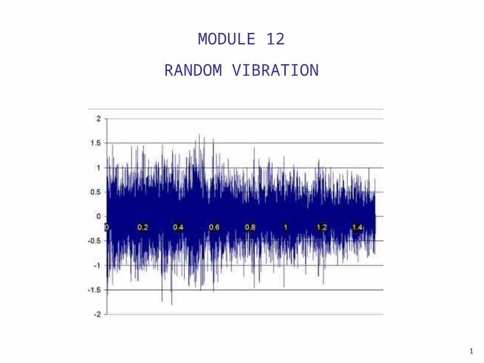
For this reason, results of random vibrations analysis are given in the form of Root Mean Square

(RMS) values. To explain the concept of RMS value, refer to graph on the next slide which shows

acceleration time history (acceleration as a function of time) of random vibration expressed in

gravitational acceleration [G].

RANDOM VIBRATION

3

Time [s]

Acceleration [G]

An example of acceleration time history data collected during 1.5s

Considering the sampling rate of 5000 samples per second, this time history curve

contains 7500 data. The overall mean value of acceleration time history GRMS2 is 0.27G2.

The overall root square of overall GRMS2 = 0.27G2 is GRMS = 0.52G

Random vibration is composed of a continuous spectrum of frequencies. The huge

amount of time history data makes it impractical to run a dynamic time analysis.

RANDOM VIBRATION

4

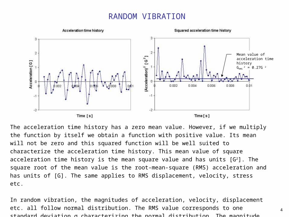
The acceleration time history has a zero mean value. However, if we multiply the function by itself we

obtain a function with positive value. Its mean will not be zero and this squared function will be well

suited to characterize the acceleration time history. This mean value of square acceleration time history

is the mean square value and has units [G2]. The square root of the mean value is the root-mean-

square (RMS) acceleration and has units of [G]. The same applies to RMS displacement, velocity,

stress etc.

In random vibration, the magnitudes of acceleration, velocity, displacement etc. all follow normal

distribution. The RMS value corresponds to one standard deviation σ characterizing the normal

distribution. The magnitude of acceleration, as characterized by the given acceleration time history, has

68% probability of remaining below 0.52G. Consequently, it has 32% probability of being less than

-0.52G or more than 0.52G.

Mean value of acceleration time historyGRMS

2 = 0.27G 2

RANDOM VIBRATION

5

Let’s assume that the acceleration time history in the previous slide is a stationary random process

where probability numbers characterizing do not change with time. This acceleration time history can

be used to calculate the Acceleration Power Spectral Density (PSD)* curve.

The overall GRMS2 of acceleration of random vibration is 0.27G2. However, random vibrations are

composed of a large number of frequencies. Let’s say we wish to investigate GRMS2 individually for a

number of frequencies in the range from 0 to 2000Hz. Therefore, we divide the 0-2000Hz range into

20 bins, each 100Hz wide and calculate GRMS2 characterizing each bin by filtering out all frequencies

falling outside of the bin (next slide),

* Variation of any property with respect to frequency is called “spectrum”.

ACCELERATION POWER SPECTRAL DENSITY

6

GRMS2 = 0.16

GRMS2 = 0.30

GRMS2 = 0.19

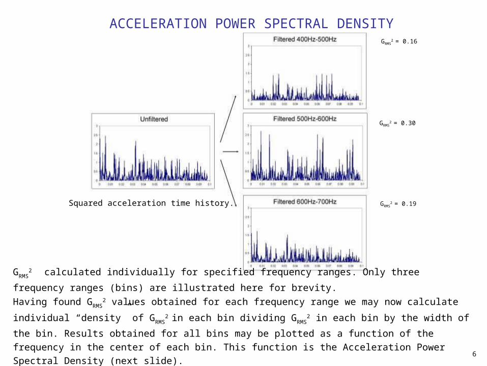
GRMS2 calculated individually for specified frequency ranges. Only three frequency ranges (bins) are

illustrated here for brevity.

Having found GRMS2 values obtained for each frequency range we may now calculate individual “density” of

GRMS2 in each bin dividing GRMS

2 in each bin by the width of the bin. Results obtained for all bins may be

plotted as a function of the frequency in the center of each bin. This function is the Acceleration Power

Spectral Density (next slide).

Squared acceleration time history.

ACCELERATION POWER SPECTRAL DENSITY

7

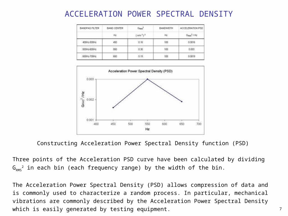
Constructing Acceleration Power Spectral Density function (PSD)

Three points of the Acceleration PSD curve have been calculated by dividing GRMS2 in each bin (each

frequency range) by the width of the bin.

The Acceleration Power Spectral Density (PSD) allows compression of data and is commonly used to

characterize a random process. In particular, mechanical vibrations are commonly described by the

Acceleration Power Spectral Density which is easily generated by testing equipment.

ACCELERATION POWER SPECTRAL DENSITY

8

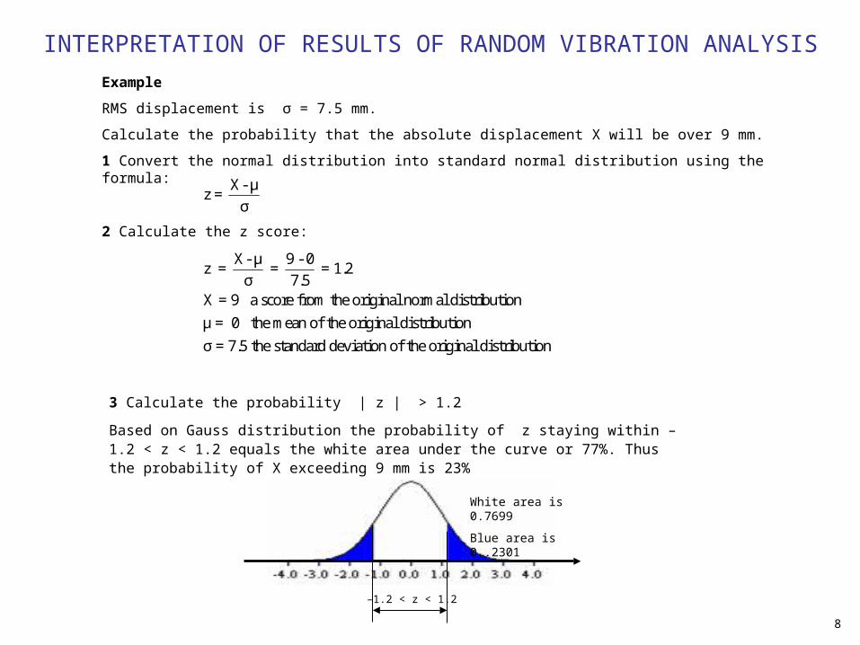
X- μ 9 - 0z = = = 1.2

σ 7.5X = 9 a score from the original normal distribution

μ = 0 the mean of the original distribution

σ = 7.5 the standard deviation of the original distribution

X- μz =

σ

2 Calculate the z score:

3 Calculate the probability | z | > 1.2

Based on Gauss distribution the probability of z staying within –1.2 < z < 1.2 equals the white area under the curve or 77%. Thus the probability of X exceeding 9 mm is 23%

Example

RMS displacement is σ = 7.5 mm.

Calculate the probability that the absolute displacement X will be over 9 mm.

1 Convert the normal distribution into standard normal distribution using the formula:

–1.2 < z < 1.2

White area is 0.7699

Blue area is 0..2301

INTERPRETATION OF RESULTS OF RANDOM VIBRATION ANALYSIS

9

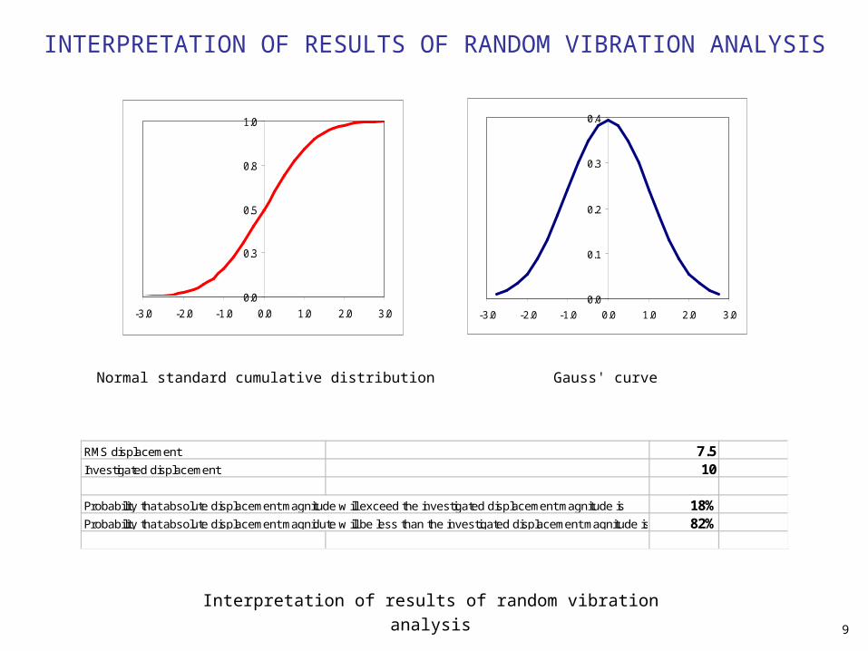
RMS displacement 7.5Investigated displacement 10

Probability that absolute displacement magnitude w ill exceed the investigated displacement magnitude is 18%Probability that absolute displacement magnidute w ill be less than the investigated displacement magnitude is 82%

0.0

0.3

0.5

0.8

1.0

-3.0 -2.0 -1.0 0.0 1.0 2.0 3.00.0

0.1

0.2

0.3

0.4

-3.0 -2.0 -1.0 0.0 1.0 2.0 3.0

Normal standard cumulative distribution Gauss' curve

Interpretation of results of random vibration analysis

INTERPRETATION OF RESULTS OF RANDOM VIBRATION ANALYSIS

10

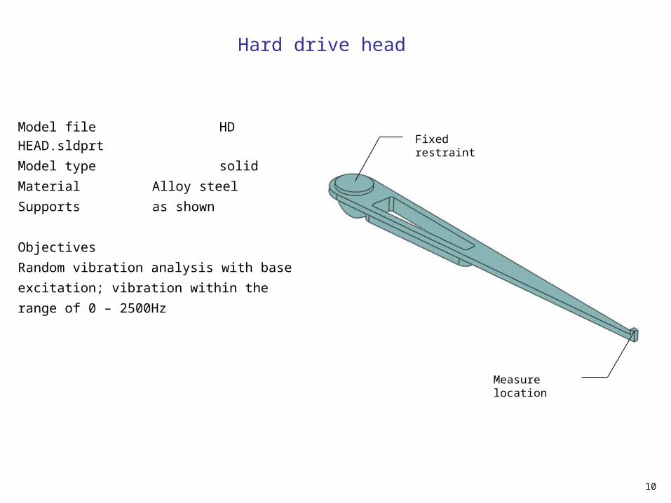
Hard drive head

Fixed restraintModel file HD HEAD.sldprt

Model type solid

Material Alloy steel

Supports as shown

Objectives

Random vibration analysis with base excitation;

vibration within the range of 0 – 2500Hz

Measure location

11

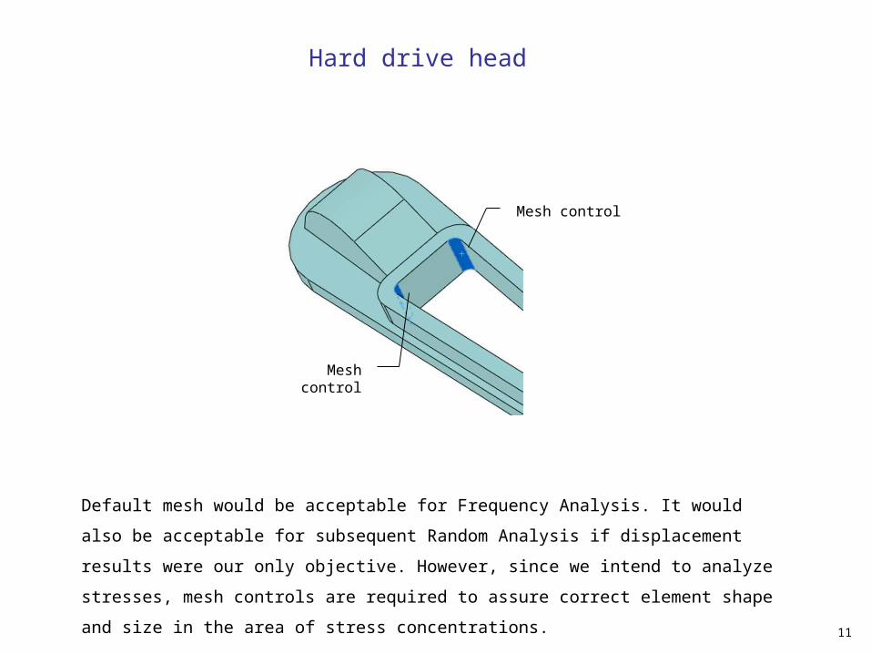
Mesh control

Meshcontrol

Default mesh would be acceptable for Frequency Analysis. It would also be acceptable for

subsequent Random Analysis if displacement results were our only objective. However, since

we intend to analyze stresses, mesh controls are required to assure correct element shape

and size in the area of stress concentrations.

Hard drive head

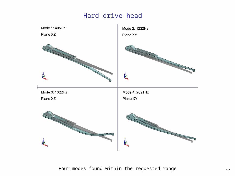
12Four modes found within the requested range

Hard drive head

13

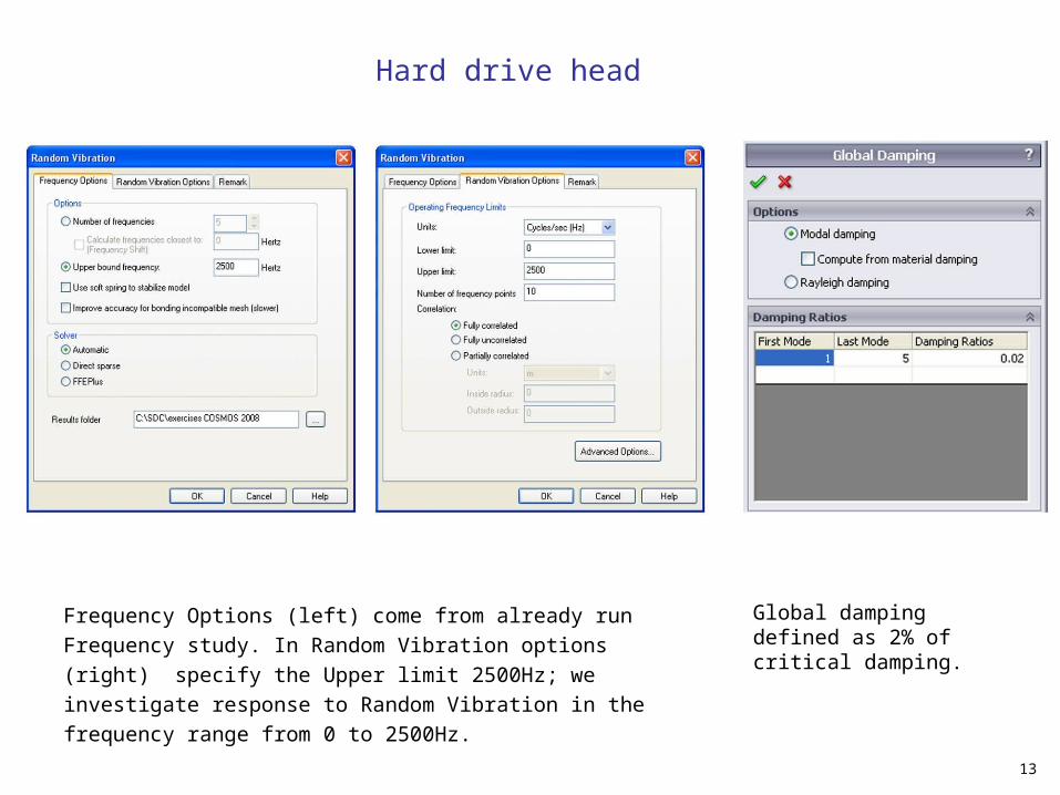
Global damping defined as 2% of critical damping.

Frequency Options (left) come from already run Frequency study. In

Random Vibration options (right) specify the Upper limit 2500Hz; we

investigate response to Random Vibration in the frequency range

from 0 to 2500Hz.

Hard drive head

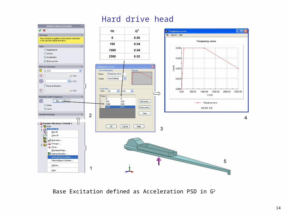
14

Base Excitation defined as Acceleration PSD in G2

Hard drive head

15

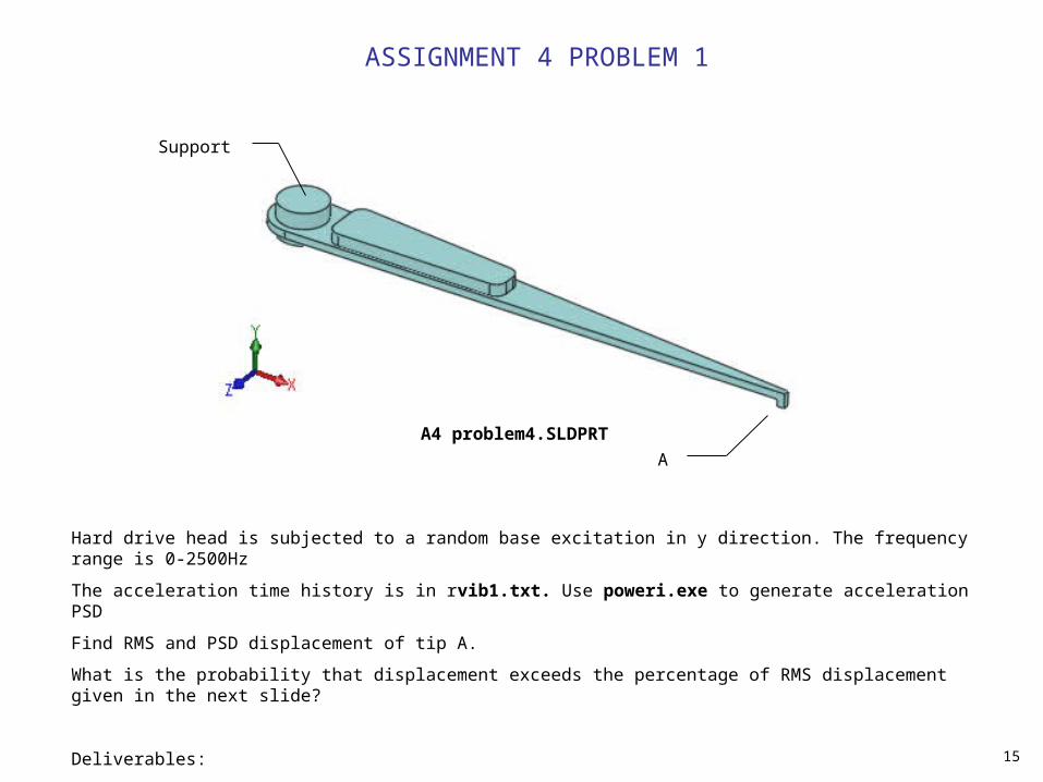
ASSIGNMENT 4 PROBLEM 1

Support

A

Hard drive head is subjected to a random base excitation in y direction. The frequency range is 0-2500Hz

The acceleration time history is in rvib1.txt. Use poweri.exe to generate acceleration PSD

Find RMS and PSD displacement of tip A.

What is the probability that displacement exceeds the percentage of RMS displacement given in the next slide?

Deliverables:

SW model with response plot and study ready to run.

A4 problem4.SLDPRT