1

Mining surprising patterns usingtemporal description length

Soumen Chakrabarti (IIT Bombay)Sunita Sarawagi (IIT Bombay)Byron Dom (IBM Almaden)

2

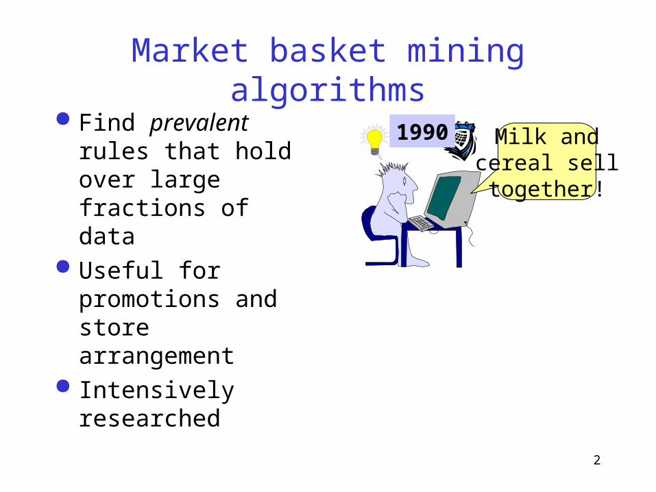
Market basket mining algorithms

Find prevalent rules that hold over large fractions of data

Useful for promotions and store arrangement

Intensively researched

1990 Milk andcereal selltogether!

3

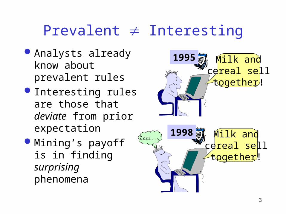
Prevalent Interesting

Analysts already know about prevalent rules

Interesting rules are those that deviate from prior expectation

Mining’s payoff is in finding surprising phenomena

1995

1998

Milk andcereal selltogether!

Zzzz... Milk andcereal selltogether!

4

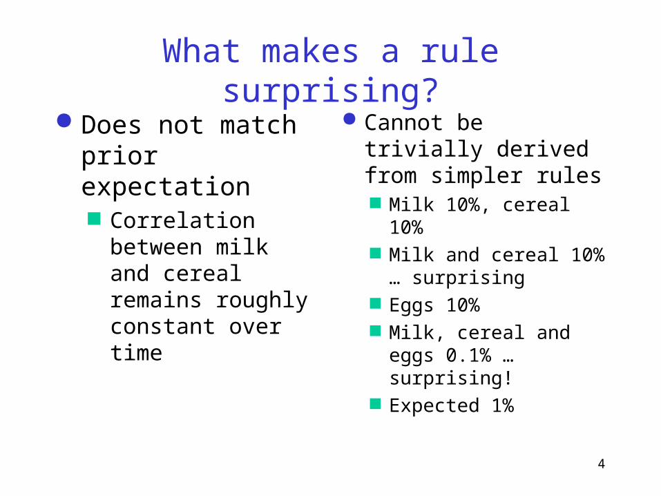
What makes a rule surprising?

Does not match prior expectation Correlation between

milk and cereal remains roughly constant over time

Cannot be trivially derived from simpler rules Milk 10%, cereal 10% Milk and cereal 10%

… surprising Eggs 10% Milk, cereal and eggs

0.1% … surprising! Expected 1%

5

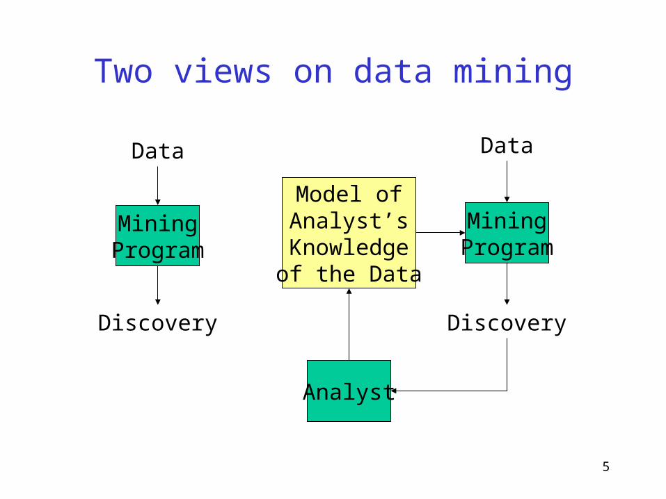
Two views on data mining

MiningProgram

Data

Discovery

MiningProgram

Data

Model ofAnalyst’s

Knowledgeof the Data

Discovery

Analyst

6

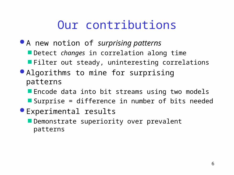
Our contributions

A new notion of surprising patterns Detect changes in correlation along time Filter out steady, uninteresting correlations

Algorithms to mine for surprising patterns Encode data into bit streams using two models Surprise = difference in number of bits needed

Experimental results Demonstrate superiority over prevalent patterns

7

A simpler problem: one item

Milk-buying habits modeled by biased coin Customer tosses this coin to decide whether

to buy milk Head or “1” denotes “basket contains milk” Coin bias is Pr[milk]

Analyst wants to study Pr[milk] along time Single coin with fixed bias is not interesting Changes in bias are interesting

8

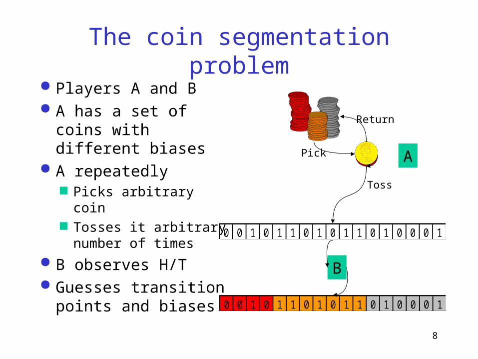
The coin segmentation problem

Players A and B A has a set of coins

with different biases A repeatedly

Picks arbitrary coin Tosses it arbitrary

number of times

B observes H/T Guesses transition

points and biases

Pick

Toss

Return

A

B

0 0 1 0 1 1 0 1 0 1 1 0 1 0 0 0 1

0 0 1 0 1 1 0 1 0 1 1 0 1 0 0 0 1

9

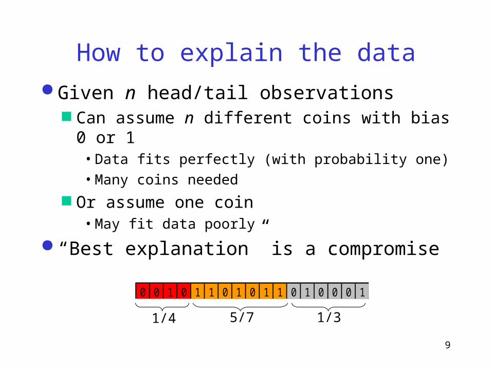
How to explain the data

Given n head/tail observations Can assume n different coins with bias 0 or 1

• Data fits perfectly (with probability one)

• Many coins needed

Or assume one coin• May fit data poorly

“Best explanation” is a compromise

0 0 1 0 1 1 0 1 0 1 1 0 1 0 0 0 1

1/4 5/7 1/3

10

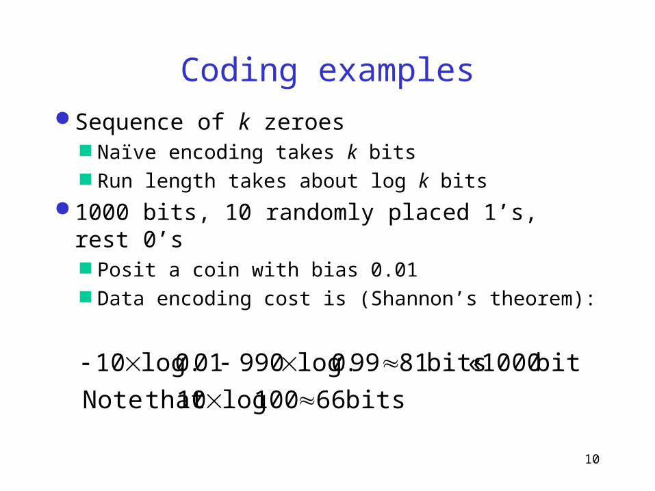
Coding examples

Sequence of k zeroes Naïve encoding takes k bits Run length takes about log k bits

1000 bits, 10 randomly placed 1’s, rest 0’s Posit a coin with bias 0.01 Data encoding cost is (Shannon’s theorem):

bits 66100log10 that Note

bits 1000 « bits 8199.0log99001.0log10

11

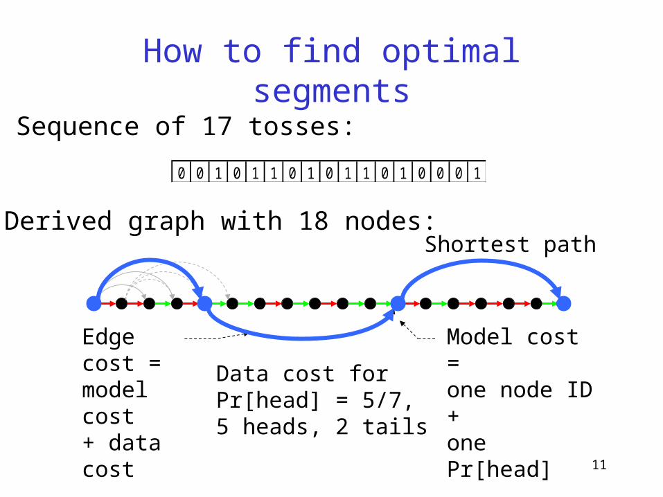
How to find optimal segments

0 0 1 0 1 1 0 1 0 1 1 0 1 0 0 0 1

Sequence of 17 tosses:

Derived graph with 18 nodes:

Edge cost = model cost+ data cost

Model cost =one node ID +one Pr[head]

Data cost forPr[head] = 5/7,5 heads, 2 tails

Shortest path

12

Approximate shortest path

Suppose there are T tosses Make T1– chunks each with T nodes

(tune ) Find shortest paths within chunks Some nodes are chosen in each chunk Solve a shortest path with all chosen nodes

13

Two or more items

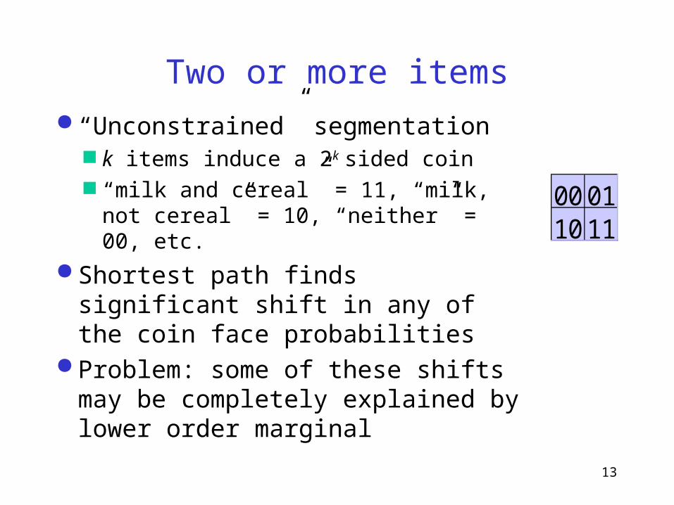
“Unconstrained” segmentation k items induce a 2k sided coin “milk and cereal” = 11, “milk, not

cereal” = 10, “neither” = 00, etc.

Shortest path finds significant shift in any of the coin face probabilities

Problem: some of these shifts may be completely explained by lower order marginal

00 0110 11

14

Example

Theta=2

0

0.1

0.2

0.3

0.4

0 2 4 6 8 10

TimeS

uppo

rtMilk Cereal Both

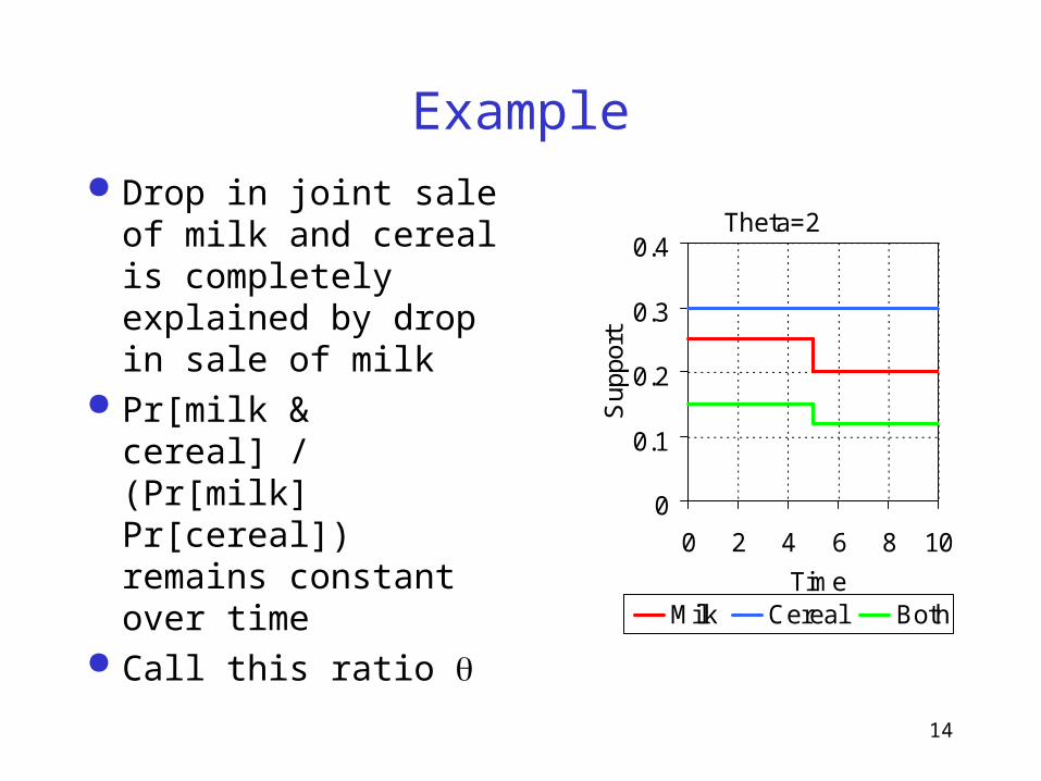
Drop in joint sale of milk and cereal is completely explained by drop in sale of milk

Pr[milk & cereal] / (Pr[milk] Pr[cereal]) remains constant over time

Call this ratio

15

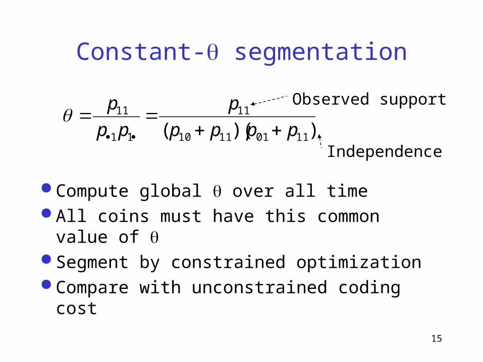
Constant- segmentation

Compute global over all time All coins must have this common value of Segment by constrained optimization Compare with unconstrained coding cost

))(( 11011110

11

11

11

pppp

p

pp

p

Observed support

Independence

16

Is all this really needed?

Simpler alternative Aggregate data into suitable time windows Compute support, correlation, , etc. in each

window Use variance threshold to choose itemsets

Pitfalls Choices: windows, thresholds May miss fine detail Over-sensitive to outliers

17

… but no simpler

Smoothing leads to an estimated trend that isdescriptive rather than analytic or explanatory.Because it is not based on an explicit probabilisticmodel, the method cannot be treated rigorouslyin terms of mathematical statistics.

The Statistical Analysis of Time SeriesT. W. Anderson

18

Experiments

2.8 million baskets over 7 years, 1987-93 15800 items, average 2.62 items per basket Two algorithms

Complete MDL approach MDL segmentation + statistical tests (MStat)

Anecdotes MDL effective at penalizing obvious itemsets

19

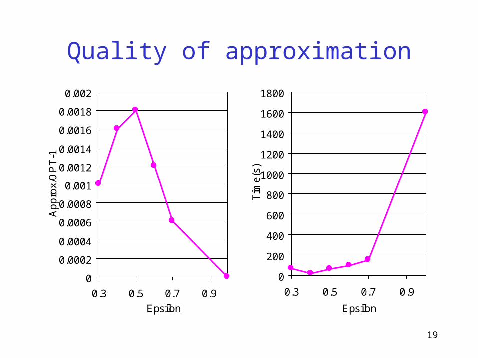
Quality of approximation

0

200

400

600

800

1000

1200

1400

1600

1800

0.3 0.5 0.7 0.9

Epsilon

Tim

e(s

)

0

0.0002

0.0004

0.0006

0.0008

0.001

0.0012

0.0014

0.0016

0.0018

0.002

0.3 0.5 0.7 0.9

Epsilon

Ap

pro

x/O

PT

-1

20

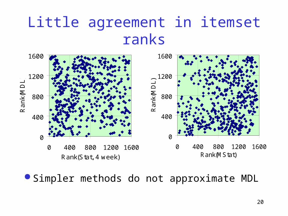
Little agreement in itemset ranks

0

400

800

1200

1600

0 400 800 1200 1600

Rank(Stat, 4 week)

Ra

nk(

MD

L)

0

400

800

1200

1600

0 400 800 1200 1600Rank(MStat)

Ra

nk(

MD

L)

Simpler methods do not approximate MDL

21

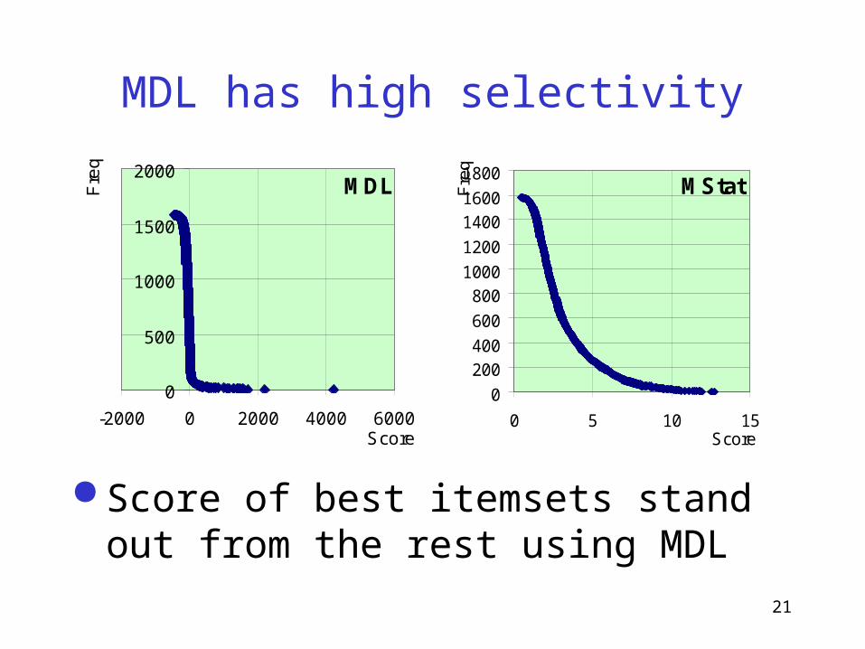
MDL has high selectivity

MDL

0

500

1000

1500

2000

-2000 0 2000 4000 6000Score

Fre

q

MStat

0

200400

600

8001000

1200

14001600

1800

0 5 10 15Score

Fre

q

Score of best itemsets stand out from the rest using MDL

22

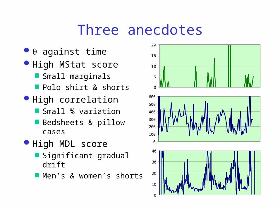
Three anecdotes

0

5

10

15

20

0

10

20

30

40

0

100

200

300

400

500

600

against time High MStat score

Small marginals Polo shirt & shorts

High correlation Small % variation Bedsheets & pillow cases

High MDL score Significant gradual drift Men’s & women’s shorts

23

Conclusion

New notion of surprising patterns based on Joint support expected from marginals Variation of joint support along time

Robust MDL formulation Efficient algorithms

Near-optimal segmentation using shortest path Pruning criteria

Successful application to real data