1

Lecture2

MGMT 650Linear Programming Applications

Chapter 4

2

Possible Outcomes of a LPPossible Outcomes of a LP(Section 2.6)(Section 2.6)

A LP is either Infeasible – there exists no solution which satisfies

all constraints and optimizes the objective function or, Unbounded – increase/decrease objective

function as much as you like without violating any constraint

or, Has an Optimal Solution Optimal values of decision variables Optimal objective function value

3

Infeasible LP – An ExampleInfeasible LP – An Example minimize

4x11+7x12+7x13+x14+12x21+3x22+8x23+8x24+8x31+10x32+16x33+5x34

Subject to x11+x12+x13+x14=100 x21+x22+x23+x24=200 x31+x32+x33+x34=150

x11+x21+x31=80 x12+x22+x32=90 x13+x23+x33=120 x14+x24+x34=170

xij>=0, i=1,2,3; j=1,2,3,4

Total demand exceeds total supply

4

Unbounded LP – An ExampleUnbounded LP – An Example

maximize 2x1 + x2

subject to

-x1 + x2 1

x1 - 2x2 2

x1 , x2 0x2 can be increased indefinitely without violating any constraint

=> Objective function value can be increased indefinitely

5

Multiple Optima – An ExampleMultiple Optima – An Example

maximize x1 + 0.5 x2

subject to

2x1 + x2 4

x1 + 2x2 3

x1 , x2 0

• x1= 2, x2=0, objective function = 2

• x1= 5/3, x2=2/3, objective function = 2

6

Marketing Application: Media SelectionMarketing Application: Media Selection

Advertising budget for first month = $30000 At least 10 TV commercials must be used At least 50000 customers must be reached Spend no more than $18000 on TV adverts Determine optimal media selection plan

Advertising Media # of potential customers reached

Cost ($) per advertisement

Max times available per month

Exposure Quality Units

Day TV 1000 1500 15 65

Evening TV 2000 3000 10 90

Daily newspaper 1500 400 25 40

Sunday newspaper 2500 1000 4 60

Radio 300 100 30 20

7

Media Selection FormulationMedia Selection Formulation Step 1: Define decision variables

DTV = # of day time TV adverts ETV = # of evening TV adverts DN = # of daily newspaper adverts SN = # of Sunday newspaper adverts R = # of radio adverts

Step 2: Write the objective in terms of the decision variables Maximize 65DTV+90ETV+40DN+60SN+20R

Step 3: Write the constraints in terms of the decision variables

DTV <= 15

ETV <= 10

DN <= 25

SN <= 4

R <= 30

1500DTV + 3000ETV + 400DN + 1000SN + 100R <= 30000

DTV + ETV >= 10

1500DTV + 3000ETV <= 18000

1000DTV + 2000ETV + 1500DN + 2500SN + 300R >= 50000

BudgetBudget

Customers Customers reachedreached

TV TV ConstraintConstraint

ss

Availability of Availability of MediaMedia

DTV, ETV, DN, SN, R >= 0DTV, ETV, DN, SN, R >= 0

Variable Value

DTV 10

ETV 0

DN 25

SN 2

R 30

Exposure = 2370 units

8

Production-Inventory ModelProduction-Inventory Model Nike produces footballs and must decide how many footballs to

produce each month over the next 6 months

Starting inventory = 5000 Production capacity each month = 30000 footballs Storage capacity = 10000 footballs Inventory holding cost of a month = 5% of production cost of that

month Determine production schedule that minimizes production and

holding cost Assume for simplicity

Production occurs continuously Demand occurs at month end

Month 1 Month 2 Month 3 Month 4 Month 5 Month 6

Demand 10000 15000 30000 35000 25000 10000

Unit cost ($) 12.50 12.55 12.70 12.80 12.85 12.95

9

Production-Inventory Model Production-Inventory Model FormulationFormulation

Step 1: define decision variables Pj = production quantity in month j Ij = end-of-month inventory in month j

Step 2: formulate objective function is terms of decision variables Sum of production cost + inventory holding cost

Step 3: formulate objective function is terms of decision variables Ij-1 + Pj = Dj + Ij

Pj < = 30000 Ij <= 10000 Pj, Ij >=0

10

Production-Inventory Formulation in LINDOProduction-Inventory Formulation in LINDO min 12.50p1+12.55p2+12.70p3+12.80p4+12.85p5+12.95p6+0.625i1+0.6275i2+0.635i3+0.64i4+0.6425i5+0.6475i6

st p1-i1=5000 Production-inventory constraint for month 1

p2+i1-i2=15000 Production-inventory constraint for month 2

p3+i2-i3=30000 Production-inventory constraint for month 3

p4+i3-i4=35000 Production-inventory constraint for month 4

p5+i4-i5=25000 Production-inventory constraint for month 5

p6+i5-i6=10000 Production-inventory constraint for month 6

p1<=30000 p2<=30000 p3<=30000 Production capacity constraints p4<=30000 p5<=30000 p6<=30000

i1<=10000 i2<=10000 i3<=10000 Inventory storage constraints i4<=10000 i5<=10000 i6<=10000

Month 1

Month 2

Month 3

Month 4

Month 5

Month 6

Demand 10000 15000 30000 35000 25000 10000

Production 5000 20000 30000 30000 25000 10000

Inventory 0 5000 5000 0 0 0

Cost = 1,535,562.00

11

Blending Problem – Self-studyBlending Problem – Self-study Ferdinand Feed Company receives four raw grains from

which it blends its dry pet food. The pet food advertises that each 8-ounce packet meets

the minimum daily requirements for vitamin C, protein and iron.

The cost of each raw grain as well as the vitamin C, protein, and iron units per pound of each grain are as follows:

Ferdinand is interested in producing the 8-ounce mixture

at minimum cost while meeting the minimum daily requirements of 6 units of vitamin C, 5 units of protein, and 5 units of iron.

Vitamin C Protein IronGrain Units/lb Units/lb Units/lb Cost/lb

1 9 12 0 0.752 16 10 14 0.93 8 10 15 0.84 10 8 7 0.7

12

Blending Problem FormulationBlending Problem Formulation

Define the decision variables

xj = the pounds of grain j (j = 1,2,3,4)

used in the 8-ounce mixture Define the objective function in terms of decision

variables

Minimize the total cost for an 8-ounce mixture:

MIN .75x1 + .90x2 + .80x3 + .70x4

13

Blending Problem - ConstraintsBlending Problem - Constraints Define the constraints

Total weight of the mix is 8-ounces (.5 pounds):

(1) x1 + x2 + x3 + x4 = .5Total amount of Vitamin C in the mix is at least 6 units:

(2) 9x1 + 16x2 + 8x3 + 10x4 >= 6Total amount of protein in the mix is at least 5 units:

(3) 12x1 + 10x2 + 10x3 + 8x4 >= 5Total amount of iron in the mix is at least 5 units:

(4) 14x2 + 15x3 + 7x4 >= 5

Nonnegativity of variables: xj > 0 for all j

14

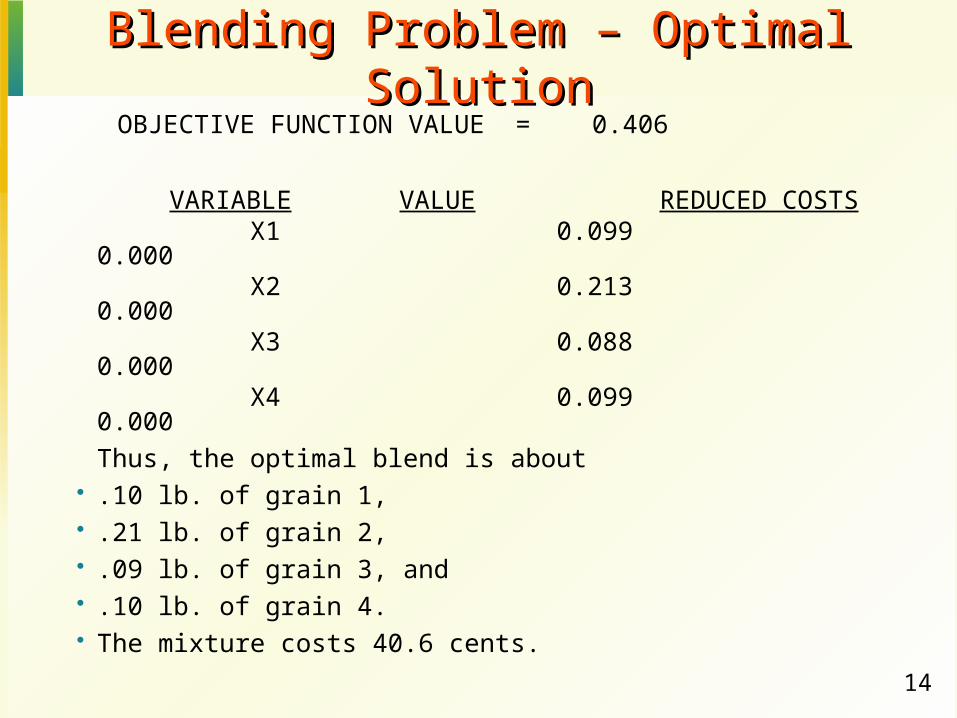
OBJECTIVE FUNCTION VALUE = 0.406

VARIABLE VALUE REDUCED COSTS X1 0.099 0.000 X2 0.213 0.000 X3 0.088 0.000 X4 0.099 0.000

Thus, the optimal blend is about .10 lb. of grain 1, .21 lb. of grain 2, .09 lb. of grain 3, and .10 lb. of grain 4. The mixture costs 40.6 cents.

Blending Problem – Optimal SolutionBlending Problem – Optimal Solution

15

Transportation Problem – Chapter 7Transportation Problem – Chapter 7 Objective:

determination of a transportation plan of a single commodity from a number of sources to a number of destinations, such that total cost of transportation is minimized

Sources may be plants, destinations may be warehouses Question:

how many units to transport from source i to destination j such that supply and demand constraints are met, and total transportation cost is minimized

16

A Transportation TableA Transportation Table

Warehouse

4 7 7 1100

12 3 8 8200

8 10 16 5150

450

45080 90 120 160

1 2 3 4

1

2

3

Factory Factory 1can supply 100units per period

Demand

Warehouse B’s demand is 90 units per period Total demand

per period

Total supplycapacity perperiod

17

LP Formulation of Transportation ProblemLP Formulation of Transportation Problem

minimize 4x11+7x12+7x13+x14+12x21+3x22+8x23+8x24+8x31+10x32+16x33+5x34

Subject to x11+x12+x13+x14=100 x21+x22+x23+x24=200 x31+x32+x33+x34=150 x11+x21+x31=80 x12+x22+x32=90 x13+x23+x33=120 x14+x24+x34=160 xij>=0, i=1,2,3; j=1,2,3,4

Supply constraint for factories

Demand constraint of warehouses

Minimize total cost of transportation

18

Solution in Management ScientistSolution in Management Scientist

Total transportation cost = 4(80) + 7(0) + 7(10)+ 1(10) + 12(0) + 3(90) + 8(110) + 8(0) + 8(0) +10(0) + 16(0) +5 (150) = $2300

19

Assignment Problem – Chapter 7Assignment Problem – Chapter 7 Special case of transportation problem

When # of rows = # of columns in the transportation tableau

All supply and demands =1 Objective: Assign n jobs/workers to n machines

such that the total cost of assignment is minimized Plenty of practical applications

Job shops Hospitals Airlines, etc.

20

Cost Table for Assignment ProblemCost Table for Assignment Problem

1 2 3 4

1 $1 $4 $6 $3

2 $9 $7 $10 $9

3 $4 $5 $11 $7

4 $8 $7 $8 $5

Pilot (i)

Aircraft (j)

All assignment costs in thousands of $

21

Formulation of Assignment ProblemFormulation of Assignment Problem minimize x11+4x12+6x13+3x14 + 9x21+7x22+10x23+9x24 +

4x31+5x32+11x33+7x34 + 8x41+7x42+8x43+5x44

subject to x11+x12+x13+x14=1 x21+x22+x23+x24=1 x31+x32+x33+x34=1 x41+x42+x43+x44=1

x11+x21+x31+x41=1 x12+x22+x32+x42=1 x13+x23+x33+x43=1 x14+x24+x34+x44=1

xij = 1, if pilot i is assigned to aircraft j, i=1,2,3,4; j=1,2,3,4 0 otherwise

Pilot Assigned to aircraft #

Cost (`000 $)

1 1 1

2 3 10

3 2 5

4 4 5Optimal Solution:

x11=1; x23=1; x32=1; x44=1; rest=0

Cost of assignment = 1+10+5+5=$21 (`000)

22

Transshipment problems are transportation problems in which a shipment may move through intermediate nodes (transshipment nodes) before reaching a particular destination node.

Transshipment Problem – Chapter 7Transshipment Problem – Chapter 7

22 22

3333

4444

5555

6666

77 77

11 11cc1313

cc1414

cc2323

cc2424

cc2525

cc1515

ss11

cc3636

cc3737

cc4646

cc4747

cc5656

cc5757

dd11

dd22

Intermediate NodesIntermediate NodesSourcesSources DestinationsDestinations

ss22

DemanDemandd

SupplSupplyy

Network Representation

23

Example: Goodyear TiresExample: Goodyear Tires The Detroit (1) and Akron (2) facilities of

Goodyear supply three customers at Memphis, Pittsburgh, and Newark.

Distribution is done through warehouses located at Charlotte (3) and Atlanta (4).

Current weekly demands by the customers are 50, 60 and 40 units for Memphis (5), Pittsburgh (6), and Newark (7) respectively.

Both facilities at Detroit and Akron can supply at most 75 units per week.

24

Transportation Costs Network Representation

ARNOLD

WASHBURN

ZROX

HEWES

7575

7575

5050

6060

4040

55

88

77

44

1155

88

33

4444

DetroitDetroit

AkronAkron

PittsburghPittsburgh

MemphisMemphis

CharlotteCharlotte

AtlantaAtlanta

NewarkNewark

25

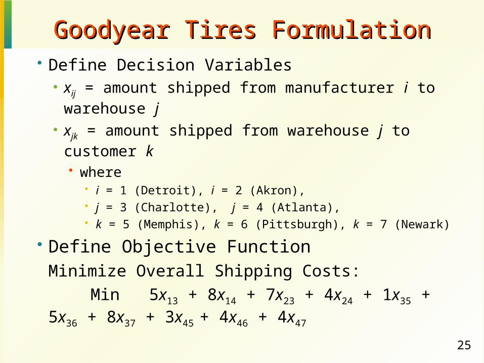
Goodyear Tires FormulationGoodyear Tires Formulation Define Decision Variables

xij = amount shipped from manufacturer i to warehouse j

xjk = amount shipped from warehouse j to customer k where

i = 1 (Detroit), i = 2 (Akron), j = 3 (Charlotte), j = 4 (Atlanta), k = 5 (Memphis), k = 6 (Pittsburgh), k = 7 (Newark)

Define Objective Function Minimize Overall Shipping Costs:

Min 5x13 + 8x14 + 7x23 + 4x24 + 1x35 + 5x36 + 8x37 + 3x45

+ 4x46 + 4x47

26

Goodyear Tires FormulationGoodyear Tires Formulation

Define Constraints

Amount Out of Detroit: x13 + x14 < 75

Amount Out of Akron: x23 + x24 < 75

Amount Through Charlotte: x13 + x23 - x35 - x36 - x37 = 0

Amount Through Atlanta: x14 + x24 - x45 - x46 - x47 = 0

Amount Into Memphis: x35 + x45 = 50

Amount Into Pittsburgh: x36 + x46 = 60

Amount Into Newark: x37 + x47 = 40

Non-negativity of variables: xij , xjk > 0, for all i, j and k.

27

Goodyear Tires SolutionsGoodyear Tires Solutions

Objective Function Value = Objective Function Value = 1150.0001150.000

VariableVariable ValueValue Reduced Reduced CostsCosts

X13 75.000 X13 75.000 0.0000.000

X14 0.000 X14 0.000 2.0002.000

X23 0.000 X23 0.000 4.0004.000

X24 75.000 X24 75.000 0.0000.000

X35 50.000 X35 50.000 0.0000.000

X36 25.000 X36 25.000 0.0000.000

X37 0.000 X37 0.000 3.0003.000

X45 0.000 X45 0.000 3.0003.000

X46 35.000 X46 35.000 0.0000.000

X47 40.000 X47 40.000 0.0000.000

28

Goodyear Tires SolutionsGoodyear Tires Solutions

ARNOLD

WASHBURN

ZROX

HEWES

7575

7575

5050

6060

4040

55

88

77

44

1155

88

33 44

44

DetroitDetroit

AkronAkron

PittsburghPittsburgh

MemphisMemphis

CharlotteCharlotte

AtlantaAtlanta

NewarkNewark

7575

7575

5050

2525

3535

4040