1 curved thin flange un equal i beams - rice · pdf file1 curved thin flange ... to utilize a...

of 23. Copyright J.E. Akin. All rights reserved.

1 Curved Thin Flange Unequal I Beams

Draft 2, 3/12/08

1.1 Introduction

Curved beams with the symmetrical shape of an “I” with unequal flange widths are very common in mechanical engineering. In addition to the “I” shape they can include the “T” shape, the inverted “T” shape, the “U” shape, the inverted “U” shape, the rectangle, and the hollow rectangle. Here the general curved beam formulation of Oden [1] is utilized with special simplifications for the restricted symmetric shapes cited above. The loadings are bending moments (Mz and My), an axial load Ns, and transverse shear loads (Vy and Vz). The TK Solver implementation reports the circumferential stresses at the inner and outer fibers, and the radial stress and transverse shear stress at the neutral axis. An extension to recover the Von Mises effective stress will be added soon.

In addition, the user can specify a specific (r, z) or (y, z) position for recovering the stress components. By filling a list of r‐coordinates plots of the stresses and geometric features can be plotted vs. radial position. Some plots will show the straight beam stresses for comparison purposes. Multiple rules for the same quantity are often used to be consistent with the different definitions used in various references. Many authors like to relate the stresses to the (pure bending) eccentricity, e. However, the eccentricity is often numerically ill‐conditioned because it can be the difference in two large numbers. Low accuracy in computing the eccentricity can cause large errors in the stress estimates.

For wide, relatively thin flanges anti‐clastic bending of those flanges reduces their effective widths and the member’s load bearing capacity. An optional “Bleich” correction is computed for the user’s consideration. Its effect will be demonstrated below. For thin webs in “T” or “U” sections you must also check for local buckling, but that relation is not included in the present model.

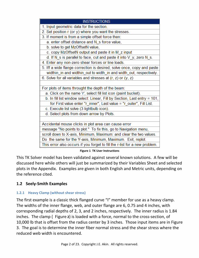
Usually you want to supply only the minimum amount of data that will uniquely define the curved beam problem. For example, in a rectangular section if you supply the width and the depth (or alternately the inner and outer radii) you do not need to calculate the area. If you did supply the area you may not have given enough digits to satisfy the TK accuracy requirements, so you may want to make the computed area a “Guess” entry. The general instructions for dealing with a curved beam model are given in Figure 1.


Figure 1 TK User Instructions

This TK Solver model has been validated against several known solutions. A few will be discussed here while others will just be summarized by their Variables Sheet and selected plots in the Appendix. Examples are given in both English and Metric units, depending on the reference cited.

1.2 Seely‐Smith Examples

1.2.1 Heavy Clamp (without shear stress)

The first example is a classic thick flanged curve “I” member for use as a heavy clamp. The widths of the inner flange, web, and outer flange are 6, 0.75 and 4 inches, with corresponding radial depths of 2, 3, and 2 inches, respectively. The inner radius is 1.84 inches. The clamp ( Figure 2) is loaded with a force, normal to the cross‐section, of 10,000 lb that is offset from the radius center by 3 inches. Those input items are in Figure 3. The goal is to determine the inner fiber normal stress and the shear stress where the reduced web width is encountered.


Figure 2 C‐clamp

Figure 3 C‐clamp geometry input and output


Note that other geometric features like the area (A), second moment terms (Jy and Jz), and centroidal radius (R) did not have to be input. Likewise, the optional input non‐dimensional measure (Z) of the inertia term Jz was computed. The point of interest (r, z) was set at (3.85, 0) to be just inside the beginning of the thin web. That input was checked against the computed radius to the web (r_web). The loading information on the section is presented in the upper part of Figure 4.

Figure 4 C‐clamp loadings and stresses

To avoid likely math errors, the most likely applied moment, due to the offset force (MzOffsetN) was calculated on the first direct solve and then copied as the input moment (M_z) before really computing the stresses. Here, high radial stresses were expected in the web. Its peak value of about 5,260 psi does exceed the inner radius normal stress of


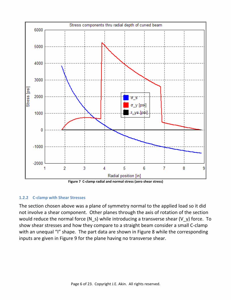
about 3,860 psi. Additional data on the neutral axis and the comparison to a straight beam are given in Figure 5. The curved and straight beam axial stress comparison results are shown in Figure 6. Increased radial stresses in the web are clearly seen in Figure 7.

Figure 5 C‐clamp neutral axis location

Figure 6 C‐clamp axial stress comparisons


Figure 7 C‐clamp radial and normal stress (zero shear stress)

1.2.2 C‐clamp with Shear Stresses

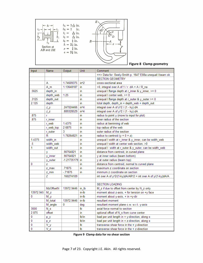
The section chosen above was a plane of symmetry normal to the applied load so it did not involve a shear component. Other planes through the axis of rotation of the section would reduce the normal force (N_s) while introducing a transverse shear (V_y) force. To show shear stresses and how they compare to a straight beam consider a small C‐clamp with an unequal “I” shape. The part data are shown in Figure 8 while the corresponding inputs are given in Figure 9 for the plane having no transverse shear.


Figure 8 Clamp geometry

Figure 9 Clamp data for no shear section


Selected stress outputs are listed in Figure 10 while the combined stresses (with no shear) are seen graphed in Figure 11.

Figure 10 Clamp stresses in no shear section


Figure 11 Stress graphs in no shear region

1.2.3 Shear plane results

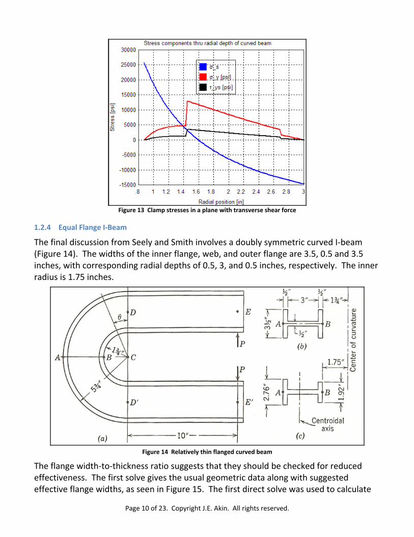
On the plane at 45 degrees from the horizontal the load reduces to equal normal and shear components. The lever arm for the bending moment is also slightly reduced. Changing those loads gives shear and normal stress results that are compared to a straight beam in Figure 12, and shown combined in Figure 13. The shear stress is much lower than the radial stress in this example.

Figure 12 Clamp section with transverse shear stress


Figure 13 Clamp stresses in a plane with transverse shear force

1.2.4 Equal Flange I‐Beam

The final discussion from Seely and Smith involves a doubly symmetric curved I‐beam (Figure 14). The widths of the inner flange, web, and outer flange are 3.5, 0.5 and 3.5 inches, with corresponding radial depths of 0.5, 3, and 0.5 inches, respectively. The inner radius is 1.75 inches.

Figure 14 Relatively thin flanged curved beam

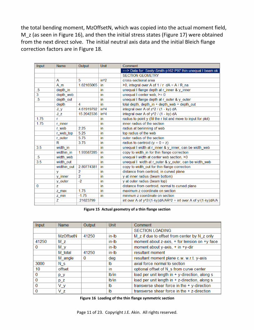
The flange width‐to‐thickness ratio suggests that they should be checked for reduced effectiveness. The first solve gives the usual geometric data along with suggested effective flange widths, as seen in Figure 15. The first direct solve was used to calculate


the total bending moment, MzOffsetN, which was copied into the actual moment field, M_z (as seen in Figure 16), and then the initial stress states (Figure 17) were obtained from the next direct solve. The initial neutral axis data and the initial Bleich flange correction factors are in Figure 18.

Figure 15 Actual geometry of a thin flange section

Figure 16 Loading of the thin flange symmetric section


Figure 17 First stress estimate on the actual section

Figure 18 Neutral axis results and suggested thin flange corrections

The Bleich correction factors are based on a thin shell analogy and agree well with experimental results showing increased stresses (around the web) resulting from less effective flanges. In the past,the correction factors were applied only once. That is, the reduced section geometry was used to find all new section properties and then a single corrected set of stress results were obtained. Since the complicated correction factors


are automated here, you can continue the corrections until the flange size change is less that some reasonable value, such as 10% of the flange width.

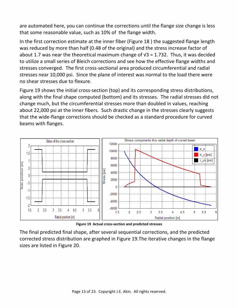
In the first correction estimate at the inner fiber (Figure 18 ) the suggested flange length was reduced by more than half (0.48 of the original) and the stress increase factor of about 1.7 was near the theoretical maximum change of √3 = 1.732. Thus, it was decided to utilize a small series of Bleich corrections and see how the effective flange widths and stresses converged. The first cross‐sectional area produced circumferential and radial stresses near 10,000 psi. Since the plane of interest was normal to the load there were no shear stresses due to flexure.

Figure 19 shows the initial cross‐section (top) and its corresponding stress distributions, along with the final shape computed (bottom) and its stresses. The radial stresses did not change much, but the circumferential stresses more than doubled in values, reaching about 22,000 psi at the inner fibers. Such drastic change in the stresses clearly suggests that the wide‐flange corrections should be checked as a standard procedure for curved beams with flanges.

Figure 19 Actual cross‐section and predicted stresses

The final predicted final shape, after several sequential corrections, and the predicted corrected stress distribution are graphed in Figure 19.The iterative changes in the flange sizes are listed in Figure 20.


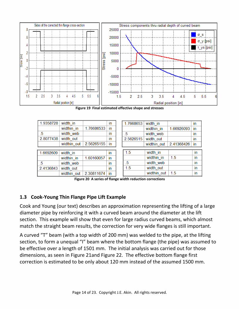
Figure 19 Final estimated effective shape and stresses

Figure 20 A series of flange width reduction corrections

1.3 Cook‐Young Thin Flange Pipe Lift Example

Cook and Young (our text) describes an approximation representing the lifting of a large diameter pipe by reinforcing it with a curved beam around the diameter at the lift section. This example will show that even for large radius curved beams, which almost match the straight beam results, the correction for very wide flanges is still important.

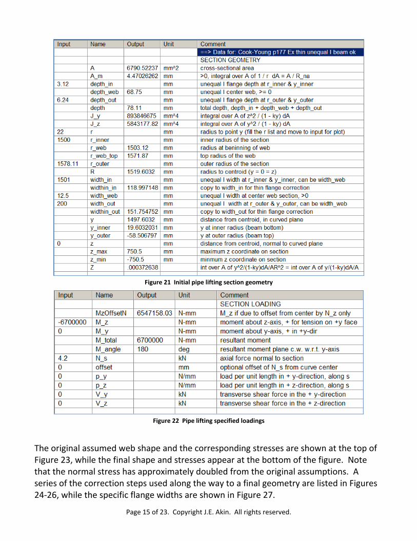
A curved “T” beam (with a top width of 200 mm) was welded to the pipe, at the lifting section, to form a unequal “I” beam where the bottom flange (the pipe) was assumed to be effective over a length of 1501 mm. The initial analysis was carried out for those dimensions, as seen in Figure 21and Figure 22. The effective bottom flange first correction is estimated to be only about 120 mm instead of the assumed 1500 mm.


Figure 21 Initial pipe lifting section geometry

Figure 22 Pipe lifting specified loadings

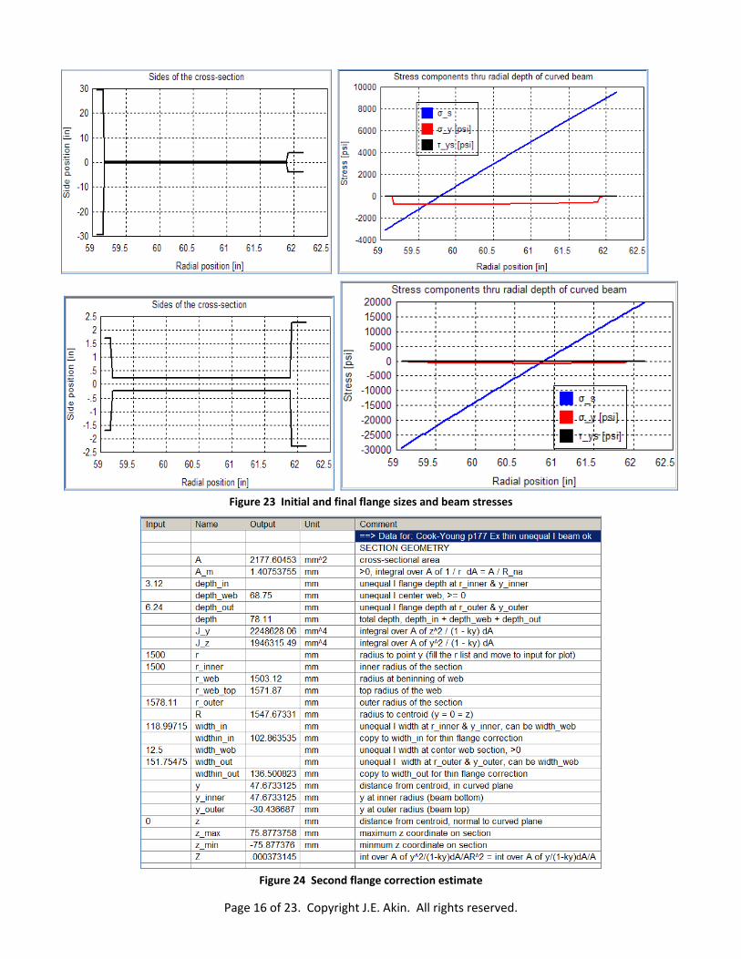
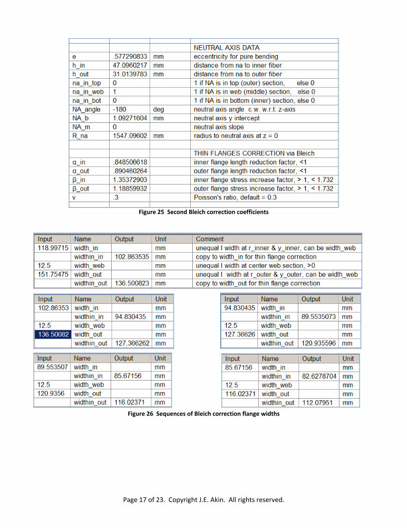
The original assumed web shape and the corresponding stresses are shown at the top of Figure 23, while the final shape and stresses appear at the bottom of the figure. Note that the normal stress has approximately doubled from the original assumptions. A series of the correction steps used along the way to a final geometry are listed in Figures 24‐26, while the specific flange widths are shown in Figure 27.


Figure 23 Initial and final flange sizes and beam stresses

Figure 24 Second flange correction estimate


Figure 25 Second Bleich correction coefficients

Figure 26 Sequences of Bleich correction flange widths


1.4 References [1‐5] 1. Cook, R.D. and W.C. Young, Advanced Mechanics of Materials. 1999: Prentice Hall. 2. Oden, J.T. and E.A. Ripperger, Mechanics of Elastic Structures. 2‐nd ed. 1981:

McGraw‐Hill. 3. Seely, F.B. and J.O. Smith, Advanced Mechanics of Materials. 2‐nd ed. 1952: John

Wiley. 4. Timoshenko, S., Strength of Materials, Part 2. 1954: Van Nostrand. 5. UTS, TK Solver User Guide. 2006, Universal Technical Systems Inc.

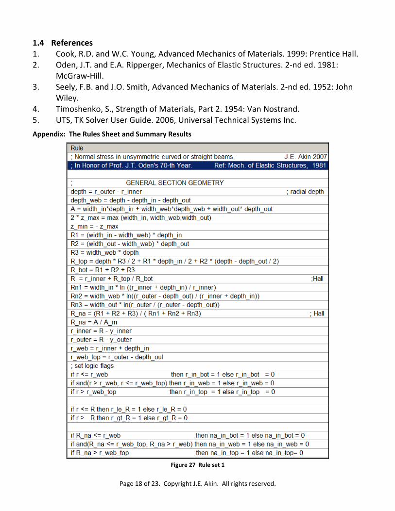
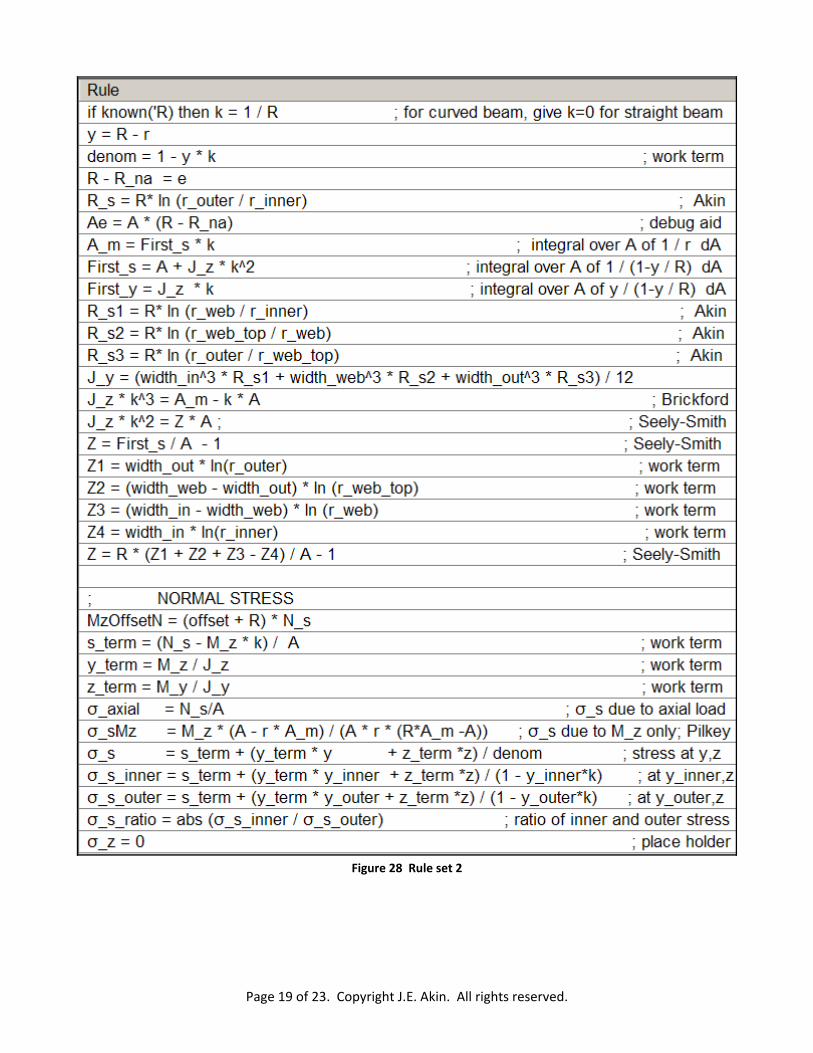
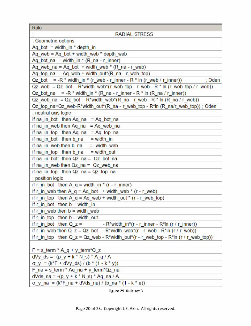
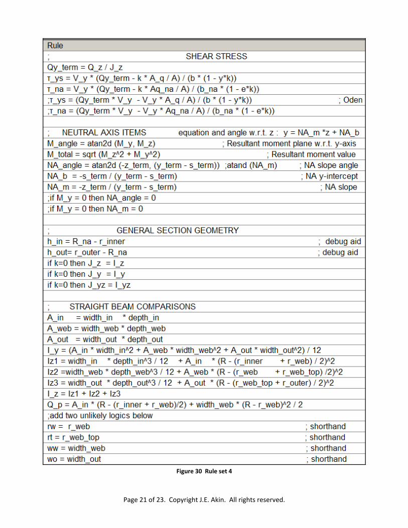
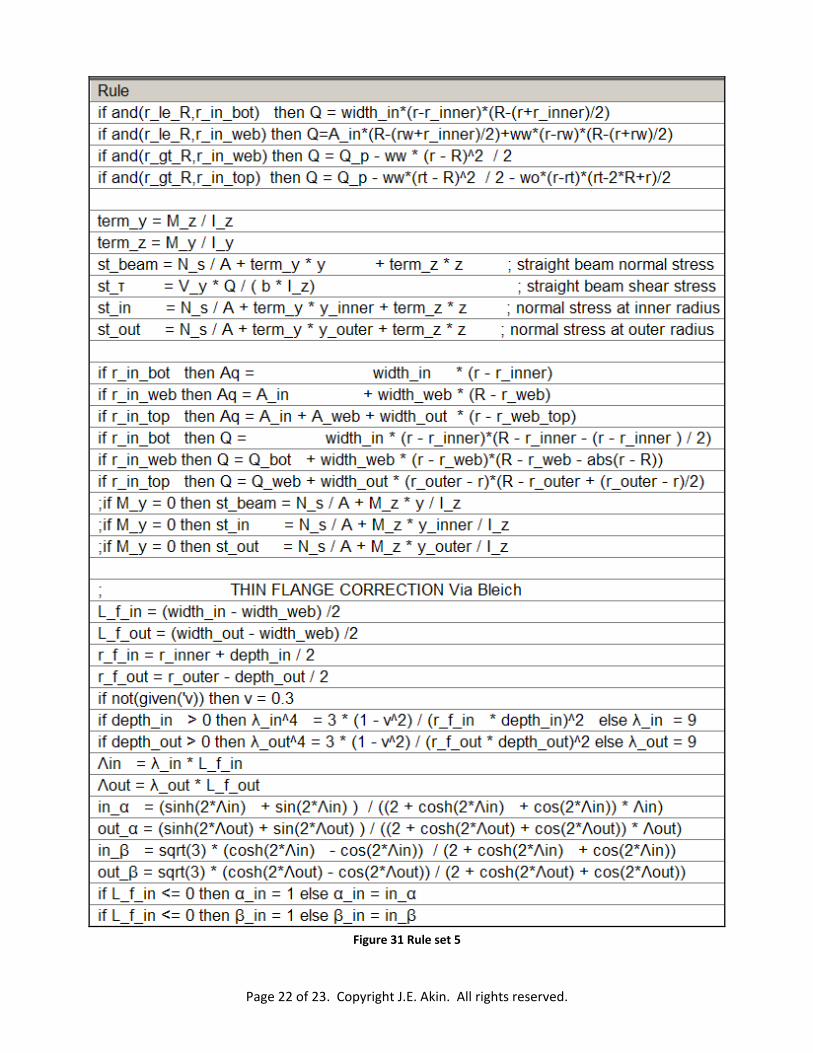
Appendix: The Rules Sheet and Summary Results

Figure 27 Rule set 1

1 curved thin flange un equal i beams - rice · pdf file1 curved thin flange ... to utilize a...

Documents