1

Chapter 9

NUMERICAL SOLUTION OF PARTIAL DIFFERENTIAL EQUATIONS

2

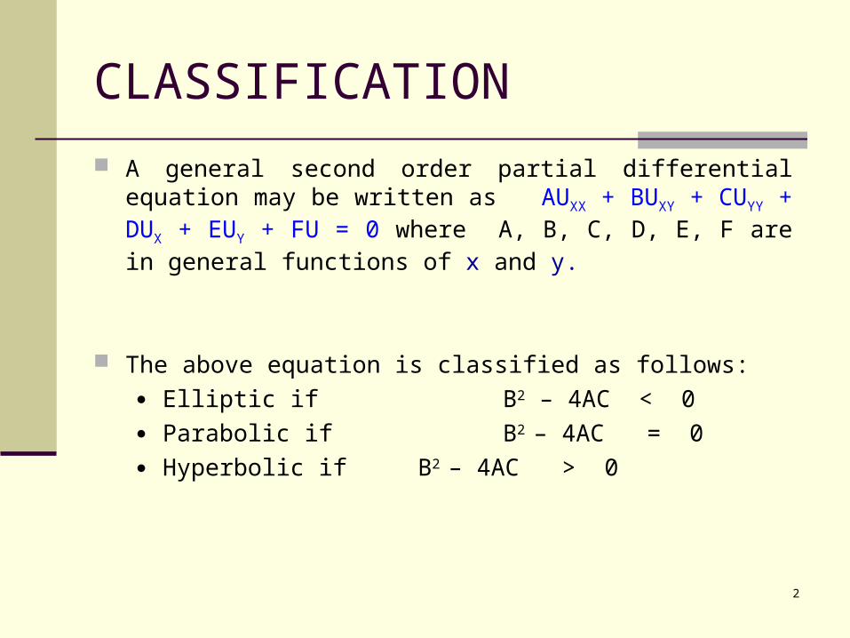
CLASSIFICATION

A general second order partial differential equation may be written as AUXX + BUXY + CUYY + DUX + EUY + FU = 0 where A, B, C, D, E, F are in general functions of x and y.

The above equation is classified as follows:● Elliptic if B2 – 4AC < 0● Parabolic if B2 – 4AC = 0● Hyperbolic if B2 – 4AC > 0

3

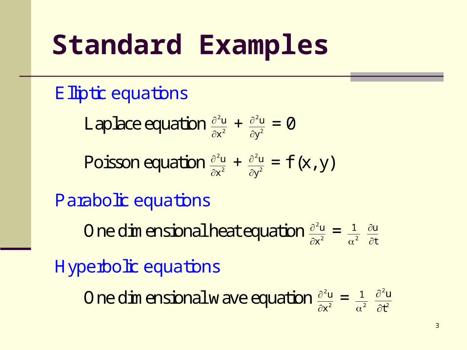
Standard Examples

Elliptic equations

Laplace equation 2

2

x

u

+

2

2

y

u

= 0

Poisson equation 2

2

x

u

+

2

2

y

u

= f (x, y)

Parabolic equations

One dimensional heat equation 2

2

x

u

=

2

1

t

u

Hyperbolic equations

One dimensional wave equation 2

2

x

u

=

2

1

2

2

t

u

4

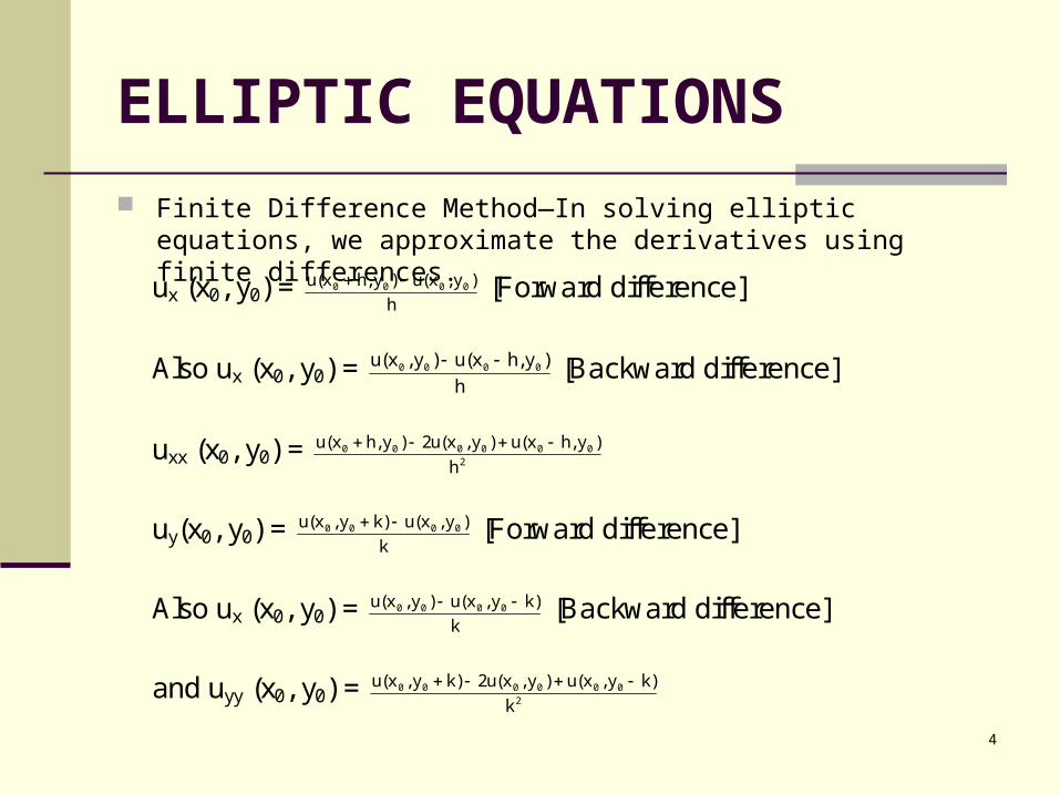
ELLIPTIC EQUATIONS

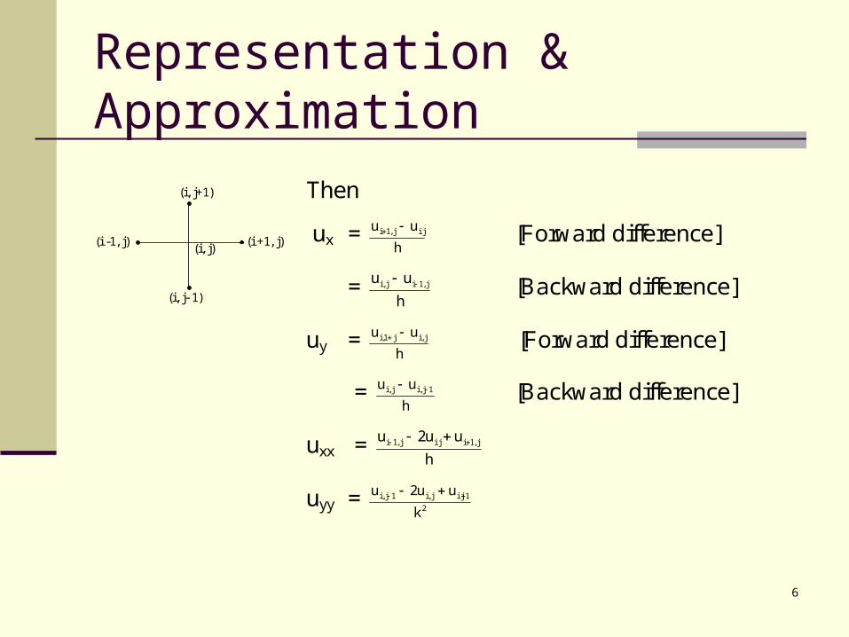
Finite Difference Method—In solving elliptic equations, we approximate the derivatives using finite differences.

ux (x0, y0) = h

)y,x(u)y,hx(u 0000 [Forward difference]

Also ux (x0, y0) = h

)y,hx(u)y,x(u 0000 [Backward difference]

uxx (x0, y0) = 2

000000

h

)y,hx(u)y,x(u2)y,hx(u

uy(x0, y0) = k

)y,x(u)ky,x(u 0000 [Forward difference]

Also ux (x0, y0) = k

)ky,x(u)y,x(u 0000 [Backward difference]

and uyy (x0, y0) = 2

000000

k

)ky,x(u)y,x(u2)ky,x(u

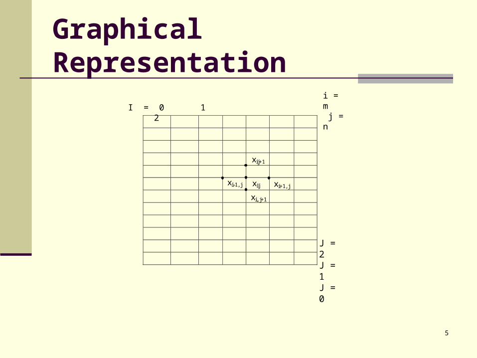
5

Graphical Representation

xij+1

xi+1, j xij xi-1, j

xi, j+1

I = 0 1 2i = m j = n

J = 2J = 1J = 0

6

Representation & Approximation

(i, j+1)

(i +1, j) (i -1, j)

(i, j- 1)

(i, j)

Then

ux = h

uu ijj,1i [Forward difference]

= h

uu j,1ij,i [Backward difference]

uy = h

uu j,ij1,i [Forward difference]

= h

uu 1j,ij,i [Backward difference]

uxx = h

uu2u j,1iijj,1i

uyy = 2

1ijj,i1j,i

k

uu2u

7

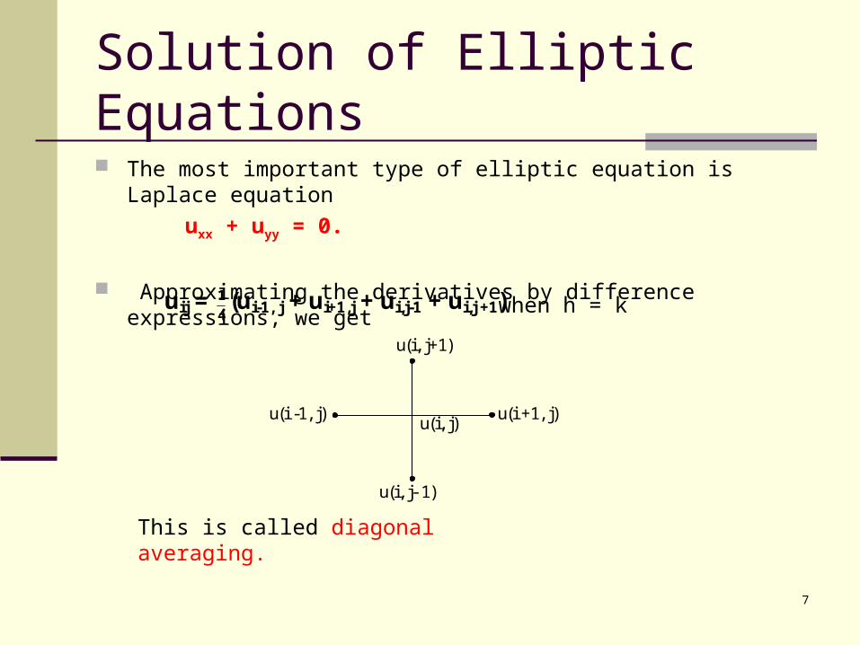
Solution of Elliptic Equations

The most important type of elliptic equation is Laplace equation

uxx + uyy = 0.

Approximating the derivatives by difference expressions, we get

uij = 4

1 (ui-1, j + ui+1,j + ui,j-1 + ui,j +1) when h = k

u(i, j+1)

u(i +1, j) u(i -1, j)

u(i, j- 1)

u(i, j)

This is called diagonal averaging.

8

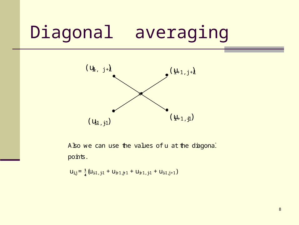
Diagonal averaging

Also we can use the values of u at the diagonal

points.

ui,j = 4

1 (ui-1, j-1 + ui+1,j+1 + ui+1, j-1 + ui-1,j +1)

(ui-1, j+1) (ui+1,j+1)

(ui-1,j-1) (ui+1,j-1)

9

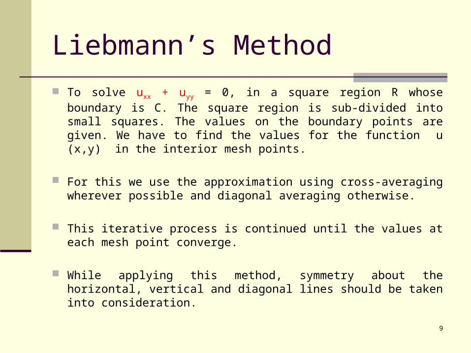
Liebmann’s Method

To solve uxx + uyy = 0, in a square region R whose boundary is C. The square region is sub-divided into small squares. The values on the boundary points are given. We have to find the values for the function u (x,y) in the interior mesh points.

For this we use the approximation using cross-averaging wherever possible and diagonal averaging otherwise.

This iterative process is continued until the values at each mesh point converge.

While applying this method, symmetry about the horizontal, vertical and diagonal lines should be taken into consideration.

10

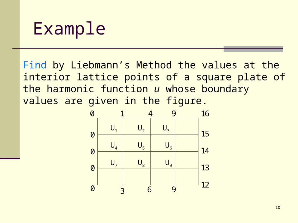
Example

0

0 12

1 4 9 16

15

14

13

3 6 9

0

0

0

Find by Liebmann’s Method the values at the interior lattice points of a square plate of the harmonic function u whose boundary values are given in the figure.

U1 U2 U3

U4 U5 U6

U7 U8 U9

11

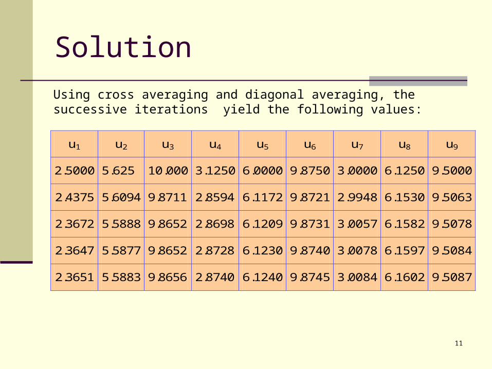
Solution

u1 u2 u3 u4 u5 u6 u7 u8 u9

2.5000 5.625 10.000 3.1250 6.0000 9.8750 3.0000 6.1250 9.5000

2.4375 5.6094 9.8711 2.8594 6.1172 9.8721 2.9948 6.1530 9.5063

2.3672 5.5888 9.8652 2.8698 6.1209 9.8731 3.0057 6.1582 9.5078

2.3647 5.5877 9.8652 2.8728 6.1230 9.8740 3.0078 6.1597 9.5084

2.3651 5.5883 9.8656 2.8740 6.1240 9.8745 3.0084 6.1602 9.5087

Using cross averaging and diagonal averaging, the successive iterations yield the following values:

12

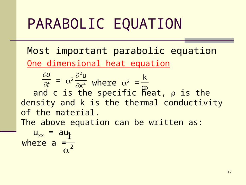
PARABOLIC EQUATION

Most important parabolic equationOne dimensional heat equation

t

u

= 2 2

2

x

u

where 2 = c

k

and c is the specific heat, is the density and k is the thermal conductivity of the material.The above equation can be written as:

uxx = aut

2

1

where a =

13

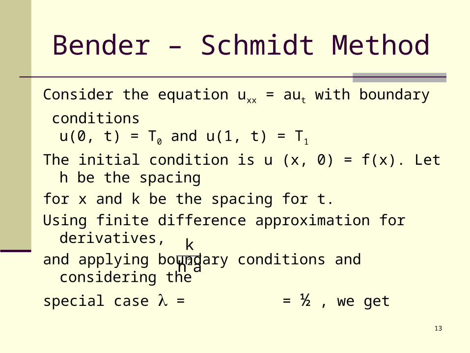
Bender – Schmidt Method

Consider the equation uxx = aut with boundary

conditions u(0, t) = T0 and u(1, t) = T1

The initial condition is u (x, 0) = f(x). Let h be the spacing

for x and k be the spacing for t.

Using finite difference approximation for derivatives,

and applying boundary conditions and considering the

special case = = ½ , we getah

k2

14

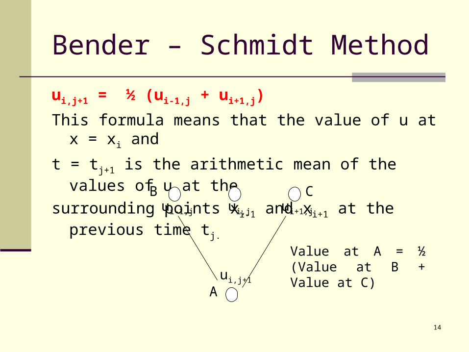
ui,j+1 = ½ (ui-1,j + ui+1,j)

This formula means that the value of u at x = xi and

t = tj+1 is the arithmetic mean of the values of u at the

surrounding points xi-1 and xi+1 at the previous time tj.

ui,j+1

A

ui+1,jui,jui-1,j

B C

Value at A = ½ (Value at B + Value at C)

Bender – Schmidt Method

15

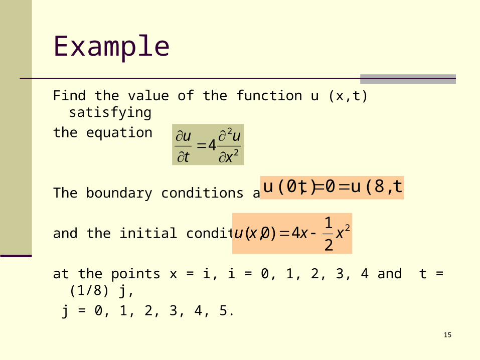
Example

Find the value of the function u (x,t) satisfying

the equation

The boundary conditions are

and the initial condition is

at the points x = i, i = 0, 1, 2, 3, 4 and t = (1/8) j,

j = 0, 1, 2, 3, 4, 5.

2

2

4x

u

t

u

2

2

14)0,( xxxu

t)(8,u 0 t)(0,u

16

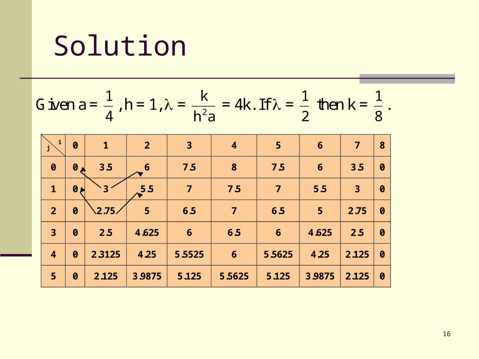
Solution

j i 0 1 2 3 4 5 6 7 8

0 0 3.5 6 7.5 8 7.5 6 3.5 0

1 0 3 5.5 7 7.5 7 5.5 3 0

2 0 2.75 5 6.5 7 6.5 5 2.75 0

3 0 2.5 4.625 6 6.5 6 4.625 2.5 0

4 0 2.3125 4.25 5.5525 6 5.5625 4.25 2.125 0

5 0 2.125 3.9875 5.125 5.5625 5.125 3.9875 2.125 0

Given a = 4

1, h = 1, =

ah

k2

= 4k. If = 2

1 then k =

8

1.

17

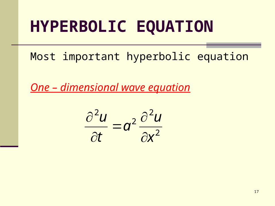
HYPERBOLIC EQUATION

Most important hyperbolic equation

One – dimensional wave equation

2

22

2

x

ua

t

u

18

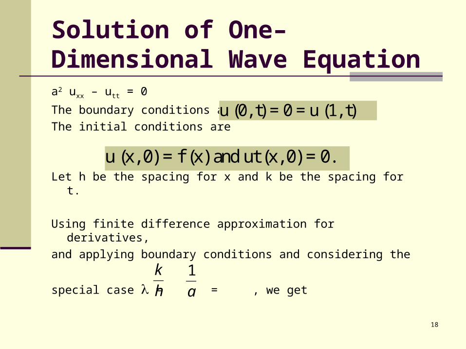
Solution of One–Dimensional Wave Equationa2 uxx – utt = 0

The boundary conditions are

The initial conditions are

Let h be the spacing for x and k be the spacing for t.

Using finite difference approximation for derivatives,

and applying boundary conditions and considering the

special case = = , we get

u (0, t) = 0 = u (1, t)

u (x, 0) = f (x) and ut (x, 0) = 0.

h

k

a

1

19

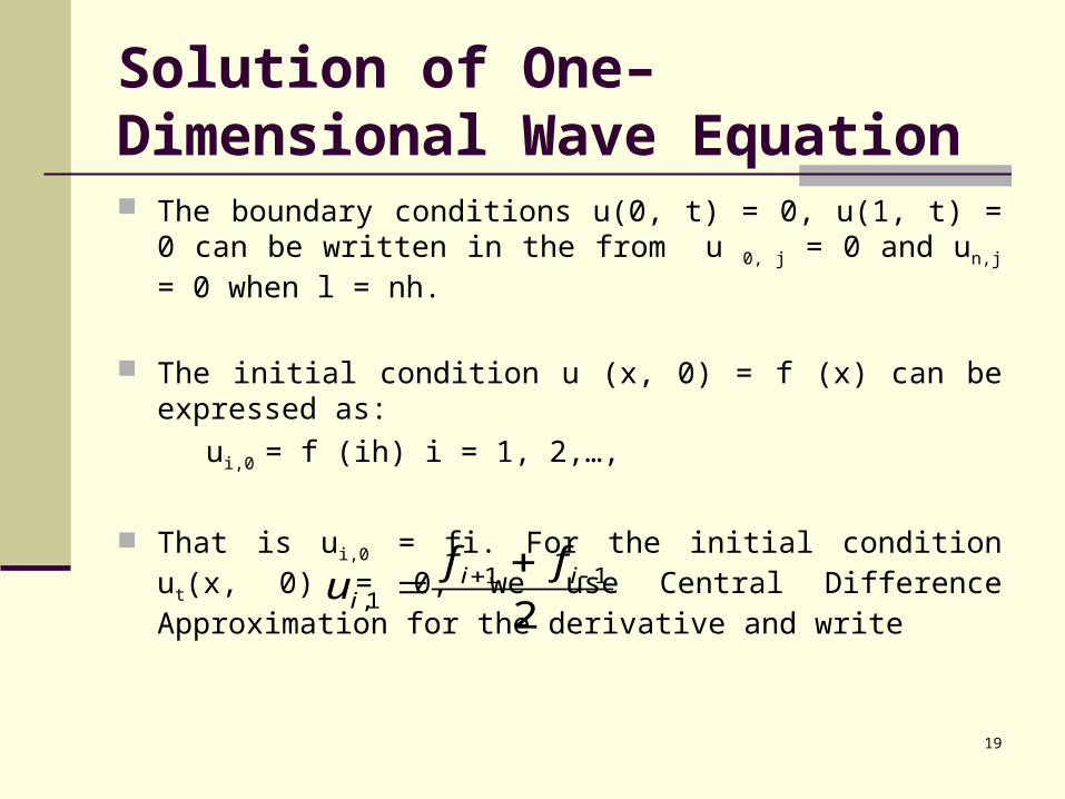
Solution of One–Dimensional Wave Equation The boundary conditions u(0, t) = 0, u(1, t) = 0 can be written in

the from u 0, j = 0 and un,j = 0 when l = nh.

The initial condition u (x, 0) = f (x) can be expressed as:

ui,0 = f (ih) i = 1, 2,…,

That is ui,0 = fi. For the initial condition ut(x, 0) = 0, we use Central Difference Approximation for the derivative and write

211

1,

iii

ffu

20

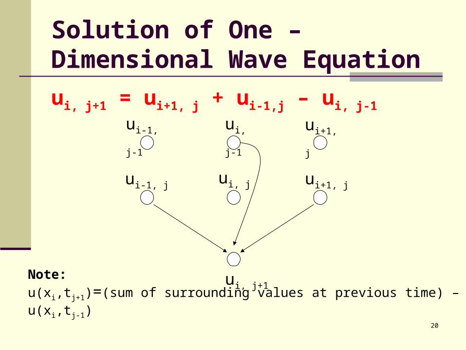
ui, j+1 = ui+1, j + ui-1,j – ui, j-1

ui-1, j-1 ui, j-1 ui+1, j

ui-1, j ui, j ui+1, j

ui, j+1Note:

u(xi,tj+1)=(sum of surrounding values at previous time) – u(xi,tj-1)

Solution of One – Dimensional Wave Equation

21

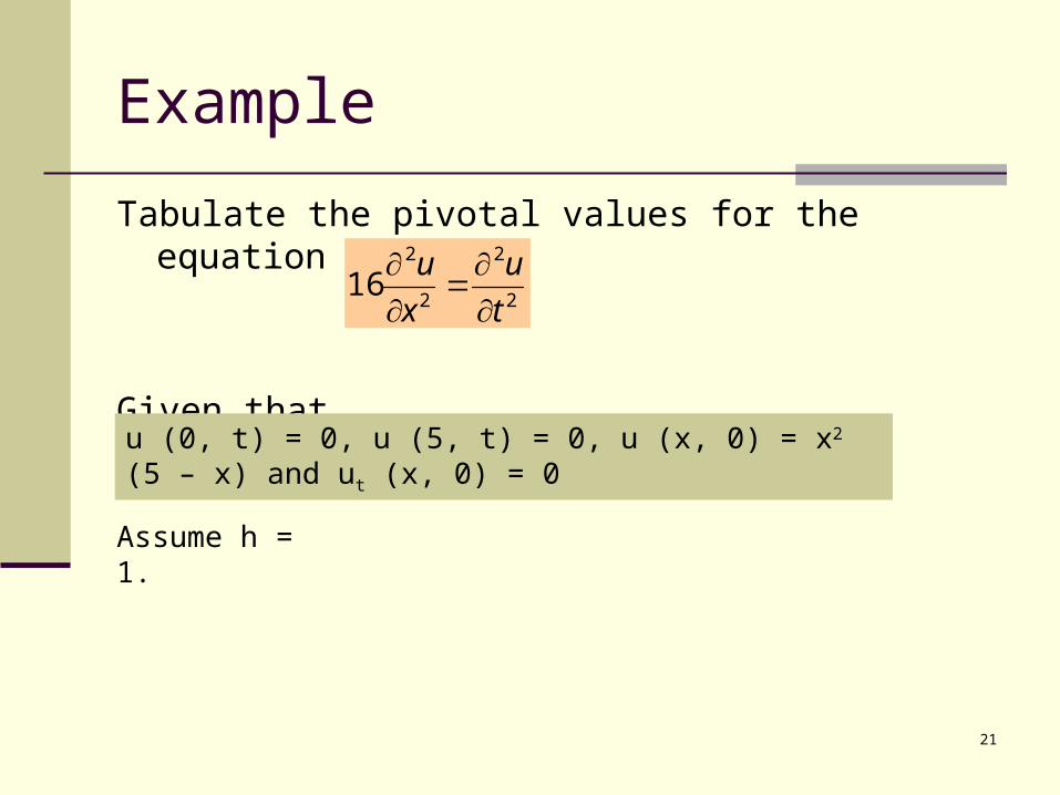
Example

Tabulate the pivotal values for the equation

Given that

2

2

2

2

16t

u

x

u

u (0, t) = 0, u (5, t) = 0, u (x, 0) = x2 (5 – x) and ut (x, 0) = 0

Assume h = 1.

22

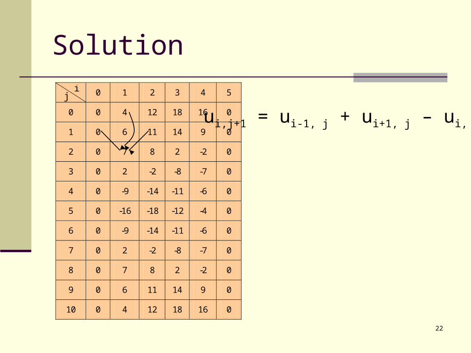
Solution

0 1 2 3 4 5

0 0 4 12 18 16 0

1 0 6 11 14 9 0

2 0 7 8 2 -2 0

3 0 2 -2 -8 -7 0

4 0 -9 -14 -11 -6 0

5 0 -16 -18 -12 -4 0

6 0 -9 -14 -11 -6 0

7 0 2 -2 -8 -7 0

8 0 7 8 2 -2 0

9 0 6 11 14 9 0

10 0 4 12 18 16 0

i j

ui,j+1 = ui-1, j + ui+1, j – ui, j-1

23

The End……

Wish you all the best…