Filtered Kernel Density Estimation

David J. Marchette1, Carey E. Priebe2, George W. Rogers1, Jeffrey L. Solka1

1Naval Surface Warfare Center, Dahlgren Div, B10Dahlgren, Virginia 22448

2Department of Mathematical SciencesThe Johns Hopkins UniversityBaltimore, Maryland 21218

Summary

A modification of the kernel estimator for density estimation is proposed which

allows the incorporation of local information about the smoothness of the density.

The estimator uses a small set of bandwidths rather than a single global one as in

the standard kernel estimator. It uses a set of filtering functions which determine

the extent of influence of the individual bandwidths. Various versions of the idea

are discussed. The estimator is shown to be consistent and is illustrated by compar-

ison to the single bandwidth kernel estimator for the case in which the filter func-

tions are derived from finite mixture models.

Keywords: Kernel Estimator, Multiple Bandwidths, Mixture Models, Density Esti-

mation.

1. INTRODUCTION

The kernel density estimator has been studied widely since its introduction in

Rosenblatt 1956 and Parzen 1962. Given i.i.d. data x1,...,xn drawn from the

unknown densityα, the standard kernel estimator (SKE) is the single bandwidth

estimator:

. (1)

See the recent books by Silverman 1986, Scott 1992 and Wand and Jones 1995 and

the bibliographies contained therein, for a good introduction to kernel estimators.

Much work has been done on selecting the optimal bandwidth h under different

assumptions onα or different optimality criteria.

Alternatively, variable bandwidth kernel estimators are of the form

, (2)

or variations on this theme. Breiman et. al. 1977, and Abramson, 1982 are early

papers in this field, while Terrel and Scott 1992 give a good discussion of the

issues of this approach. These estimators require a choice of many bandwidths,

and several approaches have been investigated. The obvious problem which may

arise in these variable bandwidth estimators is that it is not always clear how to

best incorporatea priori information about the local smoothness of the density into

these estimators. Furthermore, these estimators usually break down in the tails

where the data is sparse, and hence it is difficult to get good estimates of appropri-

ate local bandwidths.

We propose a modification to the standard kernel estimator (1), first introduced

α̂ x( ) 1nh------ K

x xi–

h------------

i 1=

n

∑=

α̂ x( ) 1n--- 1

hi----K

x xi–

hi------------

i 1=

n

∑=

in Rogers, Priebe, and Solka 1993, which uses a small number of bandwidths

instead of either extreme exemplified by equations (1) and (2).

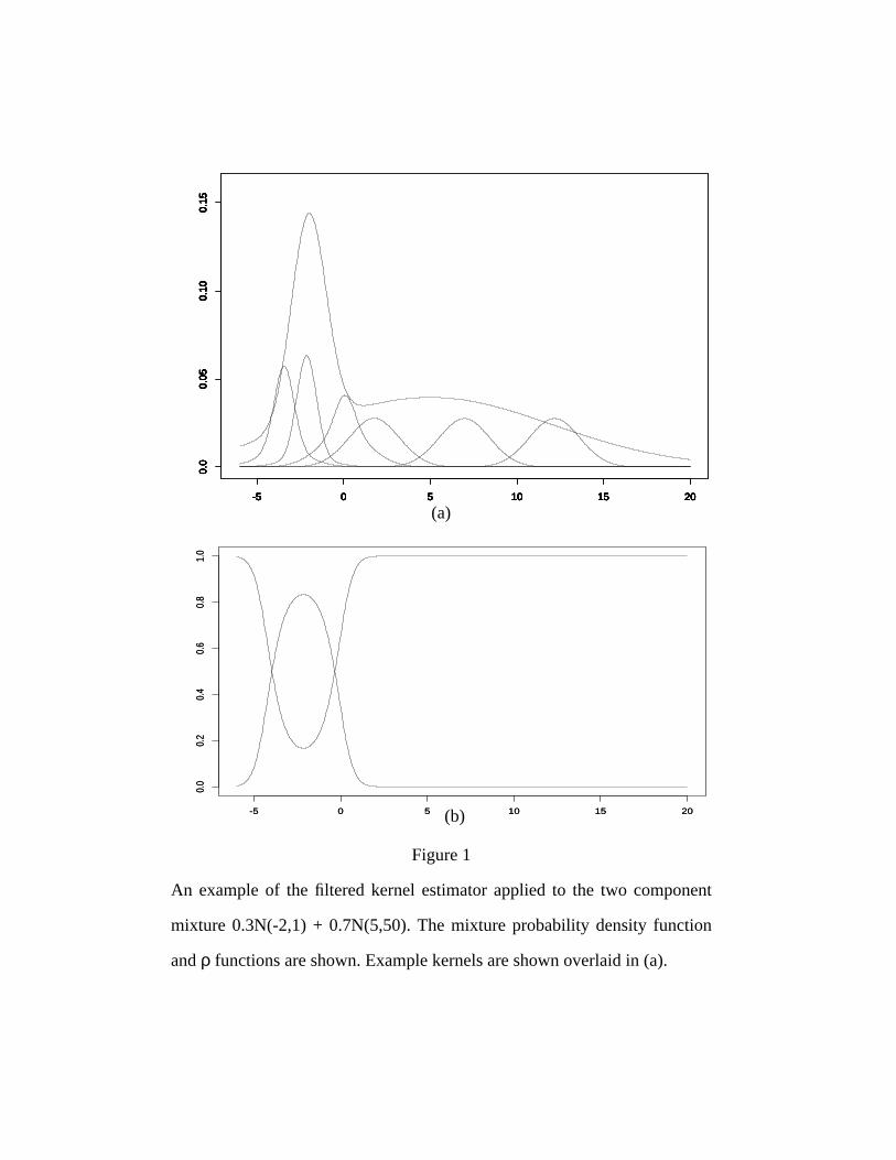
Figure 1(a) is an example of the kind of density this approach is meant to

address. The two modes of this density obviously require different bandwidths. A

single bandwidth kernel estimator must make a trade off between undersmoothing

one mode or oversmoothing the other.

Thus, we wish to have a small number of bandwidths where each bandwidth is

associated with a region of the support of the density. To this end we use a set of

functions which “filter” the data. Basically, the filter will define the extent to which

each local bandwidth is to be used for any particular data point. We can then con-

struct a kernel estimator which is a combination of the kernel estimators con-

structed using each bandwidth, with the data filtered by the filtering functions. To

be specific, consider a set of functions where 0≤ρj(x)≤1 and

(3)

for all x. Theρ functions can be interpreted as probabilities and are used to incor-

porate prior information concerning local smoothness. We will refer to theρ func-

tions as filtering functions. Associate to each filtering functionρj a bandwidth hj

such that

(4)

as n->∞. The filtered kernel estimator (FKE) for the filter is

ρj{ }j 1=

m

ρjj 1=

m

∑ x( ) 1=

0 hj<

hj 0→

nhj ∞→

ρj{ }j 1=

m

. (5)

The filtered kernel estimator was first formulated in terms of a mixture model:

given a finite mixture

(6)

the filtering functions defined by the mixture are:

. (7)

The idea is to estimate the density as a finite mixture of the form (6) and use a

bandwidth for each component which is in some sense optimal for that component

under the overall mixture model and thus vary the bandwidth according to the indi-

vidual variances of the filtering mixture. In practice, one would fit a mixture to the

data which one felt was a good representative of the local variance of the underly-

ing distribution, then use the mixture to construct bandwidths and a filtered kernel

estimator. This approach works well even when the data is not distributed as a

finite mixture, provided that the mixture captures enough of the local variance

characteristics of the data.

Figure 1(b) shows the filter functions associated with the density in Figure

1(a). For illustration, we have used the true mixture to construct the filter func-

tions. The effective kernels (the inner sum in (5)) associated with some points are

shown overlaid in Figure 1(a). The bandwidths used in this example are 0.32 and

2.1, which are appropriate for n=1000. Note that different regions have different

α̂ x( ) 1n---

ρj xi( )hj

----------------Kx xi–

hj------------

j 1=

m

∑i 1=

n

∑=

f x( ) πjfj x( )j 1=

m

∑=

ρj x( )πjfj x( )

f x( )------------------=

associated bandwidths, and that regions of overlapping filters have effective ker-

nels which are mixtures of the individual kernels. This can be seen in the third

component from the left, which has larger than normal tails.

The filtered kernel estimator does not require a finite mixture for the construc-

tion of the filtering functions, as will be seen below. Essentially any functions sat-

isfying the conditions above can be used. The purpose of the filtering functions is

to allow the user to specify the regions in which different bandwidths will operate.

We will use mixtures of normals throughout this paper for the construction of

the filtering functions for two reasons: we have some experience in finite mixture

estimation, and it is a convenient arena in which to do some comparisons with the

standard kernel estimator. There are a number of methods for choosing the number

of components to be used, either subjectively or using automated methods such as

in Priebe 1994, Solka et al 1995 or Rogers et al 1995. In this paper, we will either

assume knowledge of the true mixture (for comparison with the standard kernel

estimator) or use subjective methods.

This idea of filtering the data is similar to that used in Wand, Marron and

Rupert 1991, where the data is transformed to a known density (for example a nor-

mal) and the kernel estimator is performed there. One can think of the filters as

pulling out the data from each component and then performing a kernel estimator

on each component’s data. The advantage the filtered kernel estimator has over the

transformation approach (in our opinion) is that the relatively small number of

bandwidths give easy control over the local smoothness of the estimator, some-

thing which must be built into the transformation in the Wand, Marron and Rupert

estimator.

Note that the variable kernel estimator is a version of filtered kernel estimator:

let m=n and {Ai} be a disjoint partition of the support of the density such that Ai

intersects the data in {xi} and let

(8)

Then it is easy to see that (5) reduces to (2). The philosophy of the filtered kernel

estimator, however, is to use fewer bandwidths, and to use the information from

the estimating mixture ora priori information to choose these bandwidths.

To better illustrate this philosophy, we make the following modification of the

filtered kernel estimator (5) into an estimator with only a single bandwidth: let

, (9)

where theσj are the standard deviations of the components of (6). Thus we are let-

ting hj = hσj for a single bandwidth h. In effect what (9) does is place kernels with

different variances at different points, the variances of the kernels being tied to the

filtering mixture, and their contribution to the estimator also determined by the fil-

tering mixture. While this is slightly less general than (5) it seems to work quite

well in practice and the asymptotically optimal h can be computed in closed form,

as will be seen below.

Recent work by Hjort and Glad 1995 has considered using a parametric density

as a start on the nonparametric estimator. Given a parametric estimate the

authors define a new nonparametric estimator

. (10)

ρj xi( ) χAjxi( )=

α̂ x( ) 1n---

ρj xi( )hσj

----------------Kx xi–

hσj------------

j 1=

m

∑i 1=

n

∑=

f x θ̂,( )

f̂ x( ) 1nh------ f x θ̂,( )

f xi θ̂, -------------------K

xi x–

h------------

i 1=

n

∑=

If we assume the parametric estimator is a mixture of the form (6), we can rewrite

this as

. (11)

This is very close to the filtered kernel estimator, and it is clear that one can incor-

porate multiple bandwidths into this estimator in the same way. As the authors

point out, this works well even if the parametric estimator is quite crude, which

also holds for the filtered kernel estimator.

Although we are concerned here with univariate densities, the filtered kernel

estimator has an interesting extension to multivariate densities. Assume that the

kernel is a normal density and that the mixture (6) is a mixture of multivariate nor-

mals. For each local bandwidth hj, we associate both the posterior probabilities

from the mixture (the filtering function) and the covariance of the jth component

Σj. Thus we can take into account local structure as represented by the mixture

approximation to the density. Thus, we have the estimator:

(12)

or, in the case of (11) above,

. (13)

Clearly, this can be extended to more general kernels. This allows the use of ellip-

tical kernels which are better shaped to the local density, with different kernel

shapes in different regions of the support.

f̂ x( ) 1nh------

πjfj x( )f xi( )

------------------Kxi x–

h------------

j 1=

m

∑i 1=

n

∑=

α̂ x( ) 1n--- ρj xi( ) ϕ x xi hj

2Σj, ,

j 1=

m

∑i 1=

n

∑=

α̂ x( ) 1n--- ρj xi( ) ϕ x xi h

2Σj, ,

j 1=

m

∑i 1=

n

∑=

2. ASYMPTOTICS

Assume the conditions on the hj’s in eqn (4). Assume further that K(t) is

bounded, and a pth order kernel, that is,

(14)

Theorem 1: Under the above conditions, and assuming the existence of pth deriva-

tive of αρj, and that this derivative is in L1, the filtered kernel estimator is

L2 consistent.

pf: Recall that the mean integrated squared error (MISE) can be written as

. (15)

So the asymptotic bias is

(16)

and so the first term in (15) is

. (17)

K t( ) td∫ 1 tK t( )t 0→lim 0= =

K t( ) td∫ ∞ K2

t( ) td∫ ∞<<

trK t( ) td∫ 0 t

rK t( ) td∫ 1±==

α̂ x( )

MISE α̂( ) bias2 α̂( ) Var α̂( )+∫=

1p!----- hj

p

xp

p

dd α x( ) ρj x( )( )

j 1=

m

∑

hjphk

p

p!( ) 2--------------

k 1=

m

∑ xp

p

dd α x( ) ρj x( )( )

xp

p

dd α x( ) ρk x( )( ) xd∫

j 1=

m

∑

Letting

, (18)

we have for the second term of (15)

. (19)

Finally,

. (20)

Combining equations (17) and (19) we have

. (21)

Thus, AMISE→ 0. Note that since the standard kernel estimator is a special (triv-

ial) case of the filtered kernel estimator, this can always be made less than or equal

to the AMISE for the SKE, and with appropriate choice of the filters and band-

widths can (in many cases) improve on the performance of the SKE.

If the kernel K is the standard normal we can compute g() and obtain

. (22)

g hj hk,( ) Kthj----

Kt

hk-----

td∫=

1n---

g hj hk,( )hjhk

---------------------- ρj y( ) ρk y( ) α y( ) yd∫k 1=

m

∑j 1=

m

∑

g hj hk,( ) min hj hk,( ) sup K t( )( )≤

AMISE

hjphk

p

p!( ) 2--------------

k 1=

m

∑ xp

p

dd α x( ) ρj x( )( )

xp

p

dd α x( ) ρk x( )( ) xd∫

j 1=

m

∑ +

1n---

g hj hk,( )hjhk

---------------------- ρj y( ) ρk y( ) α y( ) yd∫k 1=

m

∑j 1=

m

∑

=

g hj hk,( ) 1

2π----------

hjhk

hj2 hk

2+----------------------=

In keeping with the ideas discussed in the introduction, we assume in this sec-

tion thatα is a mixture of normals, and that the filtering functions are generated by

the same mixture. Equation (21) then becomes

(23)

where

, (24)

. (25)

In practice we first approximate the unknown density as a mixture, then mini-

mize (23) (numerically) to calculate the bandwidths under the assumption that the

filtering density is the true density. Thus we use the optimal values for hj under the

assumption that the filtering mixture is correct. This is analogous to using a refer-

ence density such as a normal to compute the bandwidth for the standard kernel

estimator.

If instead of (5) we use (9), we have just a single bandwidth to choose, and,

again assuming thatα = f, we have:

, (26)

which is quite similar to the formula for the standard kernel estimator, and in fact

reduces to it when all the variances are equal. This can be seen by noting that

AMISE14--- Ajkh

j2hk

2

k 1=

m

∑j 1=

m

∑ 1

n 2π--------------

Bjk

hj2 hk

2+----------------------

k 1=

m

∑j 1=

m

∑+=

Ajk πjπk fj'' x( ) fk'' x( ) xd∫=

Bjk πjπk

fj x( ) fk x( )α y( )

--------------------------- xd∫=

hopt

Bjk

σj2 σk

2+

----------------------k 1=

m

∑j 1=

m

∑

2π n Ajkσj2σk

2

k 1=

m

∑j 1=

m

∑----------------------------------------------------------

1

5---

=

and

.

3. EXAMPLES

We compare the AMISE of the FKE with the standard kernel estimator with h

chosen optimally. When simulations are performed, the bandwidths are chosen by

numerically minimizing (23) or by using (26). Following Wand, Marron, and

Ruppert 1991, we compute the efficiency of the estimator as AMISEFKE/

AMISESKE so small values of the efficiency correspond to better estimates with

the FKE. For both the SKE and the FKE the true mixture is used to compute the

optimal bandwidth(s). Thus, the filtering mixture for these examples is also taken

to be the true mixture. This allows us to compare the two estimators in a “best

case” scenario.

For the examples on data which is not from a normal mixture, the filtering

mixture used is computed from a 2 component mixture via the EM algorithm. In

both cases the number of components is chosen by noting that the data is clearly

not distributed normally and that a 2 component mixture appears to be a

reasonable (conservative) fit to the data.

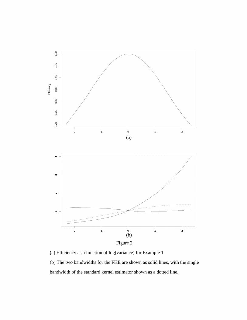
Example 1: Let , with 0.1≤ ν ≤ 10.

Figure 2(a) shows the efficiency as a function of the log of the variance. Note

that for ν ≠ 1, the FKE improves on the SKE, as one would expect. The band-

Bjkk 1=

m

∑j 1=

m

∑ 1=

Ajkk 1=

m

∑j 1=

m

∑ α''( ) 2∫=

α x( ) 12---N 0 1,( ) 1

2---N 0 v,( )+=

widths are shown in Figure 2(b), indicating that the FKE can use more appropriate

bandwidths for these densities.

This is essentially the case that the FKE was designed to address. We have a

density which is a mixture of two normals with unequal variances. As the variance

of the second term is moved away from the variance of the first term, the standard

kernel’s single bandwidth becomes less and less appropriate for the resulting den-

sity. The filtered kernel estimator allows us to take the two variances into account

in our estimator, thus improving the estimate when the variances are significantly

different.

Example 2: Marron and Wand Densities.

Marron and Wand 1992 list 15 normal mixture densities showing some of the

wide range of variations that are obtainable with simple mixtures. Table 1 shows

the efficiency of the FKE for these densities. The SKE bandwidth is chosen to be

optimal (asymptotically) under the mixture assumption. Note that the performance

of the FKE depends on the amount of local variability of the mixture, as would be

expected. The first efficiency column uses the bandwidths chosen by minimizing

the AMISEFKE numerically, while the second column shows the efficiency making

use of the variances of the components as in (9) and (26). Once again, in those

instances where the use of multiple bandwidths is appropriate, the FKE shows

improvement over the SKE. Note that it seems to make very little difference which

method is used to choose the bandwidths for the FKE.

The above examples dealt with the theoretical properties of the FKE, where the

filter is assumed to be equal to the underlying density. In practice this is not possi-

ble, and in fact if the underlying density is known any attempts at estimation are

obviously unnecessary. In the next examples we consider the case where the

underlying density is not known. In these cases we first fit a mixture to the data to

obtain a reasonable filter. Then we compute the hj under the assumption that the

filter is equal to the density. In practice, as will be seen below, this provides a good

estimator provided the filtering mixture captures most of the underlying variability

of the data.

Example 3: Wiener index of hydrocarbons.

In chemical graph theory, one wants to characterize compounds by invariants

calculated from the graphical representation of their molecular structure. The pur-

pose is to use these invariants to infer properties (boiling point, mutagenicity, etc.)

of new compounds. In this example we consider one such invariant, the Wiener

index. Information on how this is calculated, and some discussion of the problem

in general can be found in Basak et al 1995.

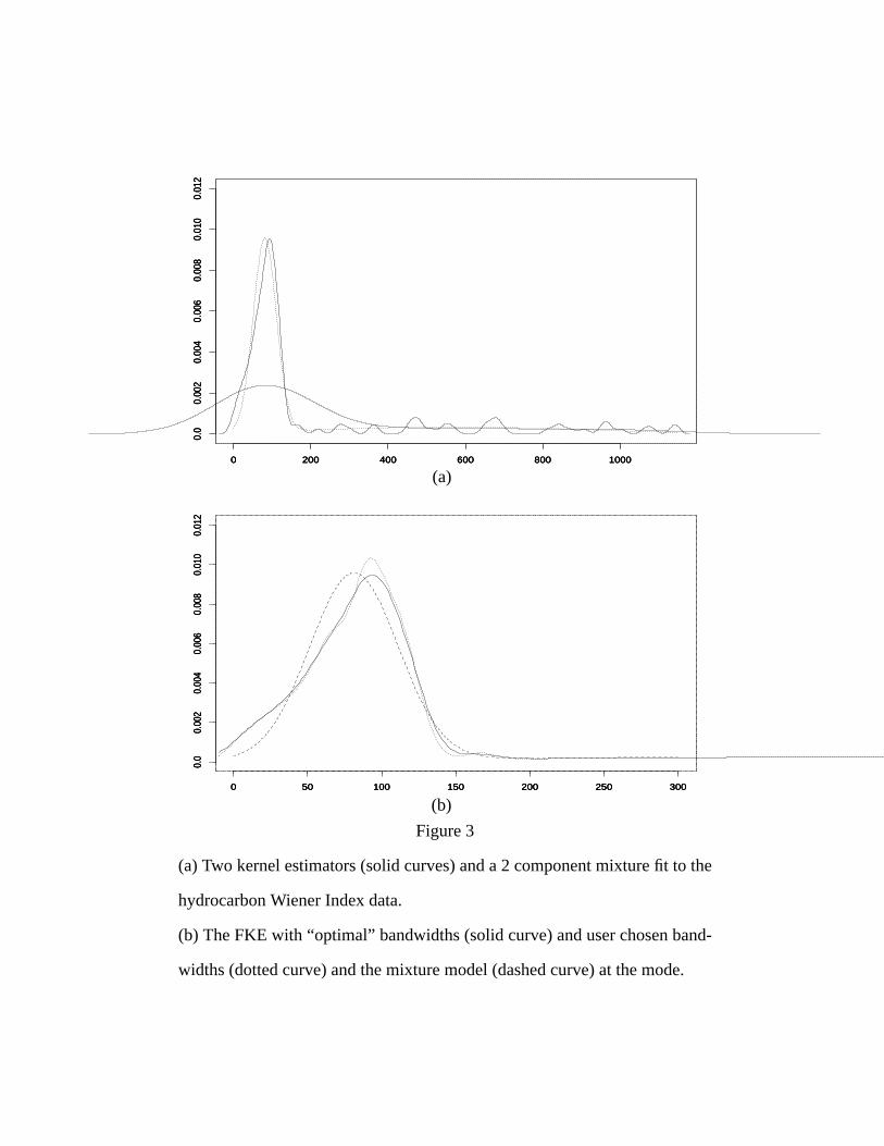
We have considered the Wiener index of 140 hydrocarbons, and have plotted

two kernel estimators (solid lines) and a two component mixture fit to the data in

Figure 3(a). Note that the data appears to be pretty well fit by the mixture model,

however the mode (consisting of approximately 70% of the data) appears to be

biased slightly to the left. Using this mixture model as our filter, we fit a filtered

kernel estimator (bandwidths 12.5 and 140.9, from (26)) to the data, and this is

presented in Figure 3(b) as the solid curve (we have focused on the main mode in

this figure). The mixture model is represented as the dashed line. Note that the ker-

nel estimator does appear to demonstrate a non-normal structure at the mode. Out-

side this range, the kernel estimator and the mixture agree pretty well, although the

kernel estimator is slightly flatter then the mixture model. It is hard with so little

data to decide between the two models on this long tail, and so we will concern

ourselves with the mode in this example.

In order to illustrate the flexibility of the FKE we have used a smaller first

bandwidth, in this case a bandwidth of 9 and plotted the result as the dotted line.

Note that the effect of this reduced bandwidth is restricted to the region below 200.

Thus, the user can adjust the smoothness of the estimator within regions indicated

by the parametric approximation, without having a large effect on other regions of

the density. It seems that the default bandwidths have done a pretty good job on

this density. We would not argue that the smaller bandwidth is more appropriate in

this case, but merely include it to illustrate the flexibility of the FKE.

Note that in spite of the figure, we are really interested in an estimate of the

density throughout its range. Thus, one cannot simply truncate the data and esti-

mate the density of the truncated data. The FKE gives us a function which is an

estimate of the density, not just a sequence of plots which require the mental

smoothing of some regions, which is what a standard kernel estimator is forced to

do in many cases.

Example 4: Lognormal.

100 data points were drawn from a lognormal and a two component mixture

was fit to the data using the EM method (see, e.g., Titterington, Smith, and Makov

1985). The bandwidths for the filtered kernel estimator were chosen assuming the

filter to be equal to the true density. Thus we first construct the mixture estimate

and then use the bandwidths that would be optimal for that mixture density, in

much the same way that one might use a normal or some other density as a refer-

ence estimate for the standard kernel estimator.

Figure 4(a) shows the density estimates for the standard kernel estimator and

the FKE. The bandwidths for the FKE were h1 = 0.4 and h2 = 2.2. The bandwidth

for the standard kernel estimator was chosen by hand to get a reasonable fit to the

true density. The plot shown uses a value of 0.3 for the bandwidth of the standard

kernel. Note that the FKE smooths the tail without over smoothing the mode. As in

the Hydrocarbon data example we can decrease the first bandwidth to move the

FKE closer to the SKE at the mode without effecting the smoothness of the tail, if

this were desirable.

Figure 4(b) compares the density estimates of the FKE and the filtering mix-

ture. The FKE is a better fit than the filtering mixture. It could be argued that this is

in part due to the choice of filtering mixture, and that a mixture of 3 or 4 terms

could do much better. This is true, provided the number of terms did not get too

large (recall this data set contains only 100 points). However, the point is that the

FKE has the ability to overcome the shortcomings of the filtering mixture, and

hence acts as a hedge against misspecification of the mixture. In fact, it is possible

to use the results of the FKE as feedback to the filtering mixture to increase the

number of terms (see Rogers et al 1995 for some preliminary work in this area).

4. DISCUSSION

The filtered kernel estimator is superior in performance to the standard kernel

estimator, provided appropriate filter functions and bandwidths can be chosen. In

section 2 it was shown that any reasonable filter functions will give asymptotic

performance no worse than the standard single bandwidth kernel estimator. This is

no surprise, since the single bandwidth kernel estimator is a special case of the fil-

tered kernel.

It would seem at first that the added trouble of selecting filtering functions and

bandwidths would make the estimator difficult to use in practice. However the idea

of using a finite mixture fit to the data to construct the filters is one which appears

to work well in a variety of situations, even those for which the data is not drawn

from a finite mixture. The ability to take local structure into account is a powerful

one which will allow much better estimates in those situations where there is rea-

son to believe the local structure is justified. Experience has shown that good

results are obtained even with a very crude estimate from the mixture model.

We suggest that in using this approach one should start with a very conserva-

tive estimate of the number of components. This will tend to give good results, and

will not have the problems associated with overfitting the mixture model. In an

exploratory data analysis mode one could then increase the number of components

of the mixture model if the FKE seemed to indicate this was appropriate.

It should be noted that bad filters can produce bad FKE’s. This is not unreason-

able, however it does mean that care must be used in the choice of the filtering

mixture. Just as the standard kernel estimator produces errors when the bandwidth

is taken to be too large or too small, mixtures which have terms which are not sup-

ported by the data will produce local errors in the FKE estimate. This local charac-

ter of the estimator gives some protection, since the effect of the error is reduced

outside the region in which the corresponding filter function dominates. This is in

contrast to the single kernel estimator where the choice of the bandwidth has a glo-

bal effect.

The possibility of using the filtered kernel estimator to aid in choosing a mix-

ture estimate of the density, as mentioned above, is quite interesting. Work on

automated procedures to do this is ongoing, and preliminary results are reported in

Rogers et al 1995.

As was noted in the introduction, we do not view the filtered kernel estimator

as a version of a variable bandwidth kernel estimator of the kind in (2). However,

the basic philosophy of using the components of a mixture to determine the band-

widths could be adopted for variable kernel estimators. Consider instead of having

a single bandwidth hj for each component, having multiple bandwidths hij = hj/

sqrt(fj(xi)). Note that we still only have m bandwidths, the hj, to choose, the rest

coming immediately from the filter and the data. It is not obvious that this is an

improvement over the traditional variable bandwidth estimators, using the filtering

mixture as the pilot estimate for example, except that it retains the ability to easily

change the estimate locally without effecting other regions. In the case of the fil-

tered kernel estimator this is done by changing just one of the hj’s, as was demon-

strated in the hydrocarbon data example. One can do this with the standard version

of the variable kernel estimator in principle, but with quite a bit more work.

We have used mixtures to construct the filtering functions, and have shown that

this works well in practice. It would be interesting to see if one could craft the fil-

tering functions by hand, perhaps with a graphical interface to draw the functions.

This might be a useful tool for data analysis. It is not obvious that the best filters

are obtained from mixtures, even in the case that the density is a mixture, and more

work is needed in this area.

Finally, we have focused on the univariate case in this work, but other exten-

sions are possible. The multivariate version of the FKE has much promise, and

will be addressed in the future. The ability to effectively tune the kernels to the

local structure of the data will be a powerful and useful tool for multivariate den-

sity estimation. It is believed that this ability to define the structure locally will be

of use in exploratory data analysis and in discriminant analysis.

Acknowledgments

The authors would like to thank Dr. Subhash Basak for providing the hydrocar-

bon data, and Dr. Ed Wegman for comments and encouragement. We would also

like to thank the anonymous reviewers for their suggestions. This work was done

in part through Independent Research funding at the Naval Surface Warfare Cen-

ter, Dahlgren Division.

REFERENCES

Abramson, I.S. (1982), “On Bandwidth Variation in Kernel Estimates--A Square

Root Law”,The Annals of Statistics, 10, 1217-1223.

Basak, Subhash C., Grunwald, Gregory D., and Niemi, Gerald J., 1995, “Use of

graph theoretical and geometrical molecular descriptors in structure-activity

relationships”, to appear in3-D Molecular Structure and Chemical Graph The-

ory, A. T. Balaban, Ed., New York: Plenum Press.

Breiman, L., Meisel, W, and Purcell, E. (1977), “Variable Kernel Estimates of

Multivariate Densities”,Technometrics, 19,135-144.

Hjort, N.L. and Glad, I.K., (1995) “Nonparametric density estimation with a para-

metric start”,The Annals of Statistics, 23, 882-904.

Marron, J.S. and Wand, M.P. (1992), “Exact Mean Integrated Squared Error,” The

Annals of Statistics, 20, 712-736.

Parzen, E. (1962), “On Estimation of a Probability Density Function and Mode,”

Ann. Math. Statist., 33, 1065-1076.

Priebe, C.E., (1994), “Adaptive Mixtures”,Journal of the American Statical Asso-

ciation, 89, 796-806.

Rogers, G.W., Marchette, D.J., and Priebe, C.E., (1995), “A Procedure for Model

Complexity Selection in Semiparametric Mixture Model Density Estimation”,

to appear in the Proceedings of the 10th International Conference on Math. and

Computer Modelling.

Rogers, G.W., Priebe, C.E., and Solka, J.L. (1993), “Filtered Kernel Probabilistic

Neural Network,”SPIE Vol. 1962 Adaptive and Learning Systems II, 242-252.

Rosenblatt, M. (1956), “Remarks on some Nonparametric Estimates of a Density

Function,”Ann. Math. Statist., 27, 832-835.

Scott, D.W. (1992),Multivariate Density Estimation, New York: John Wiley.

Silverman, B.W. (1986),Density Estimation for Statistics and Data Analysis, New

York: Chapman and Hall.

Solka, J.L., Wegman, E.J., Priebe, C.E., Poston, W.L. and Rogers, C.W., (1995) “A

method to determine the structure of an unknown mixture using the Akaike

information criterion and the bootstrap”, unpublished manuscript.

Tapia, R.A. and Thompson, J.R. (1978),Nonparametric Probability Density Esti-

mation, Baltimore: The Johns Hopkins University Press.

Terrell, G.R. and D.W. Scott (1992), “Variable Kernel Density Estimation”,The

Annals of Statistics, 20, 1236-1265.

Titterington, D.M., Smith, A.F.M., and Makov, U.E. (1985),Statistical Analysis of

Finite Mixture Distributions, New York: John Wiley.

Wand, M.P., and Jones, M.C., 1995,Kernel Smoothing, London, Chapman &Hall.

Wand, M.P., Marron, J.S., and Ruppert, D. (1991), “Transformation in Density

Estimation,”Journal of the American Statical Association, 86, 343-361.

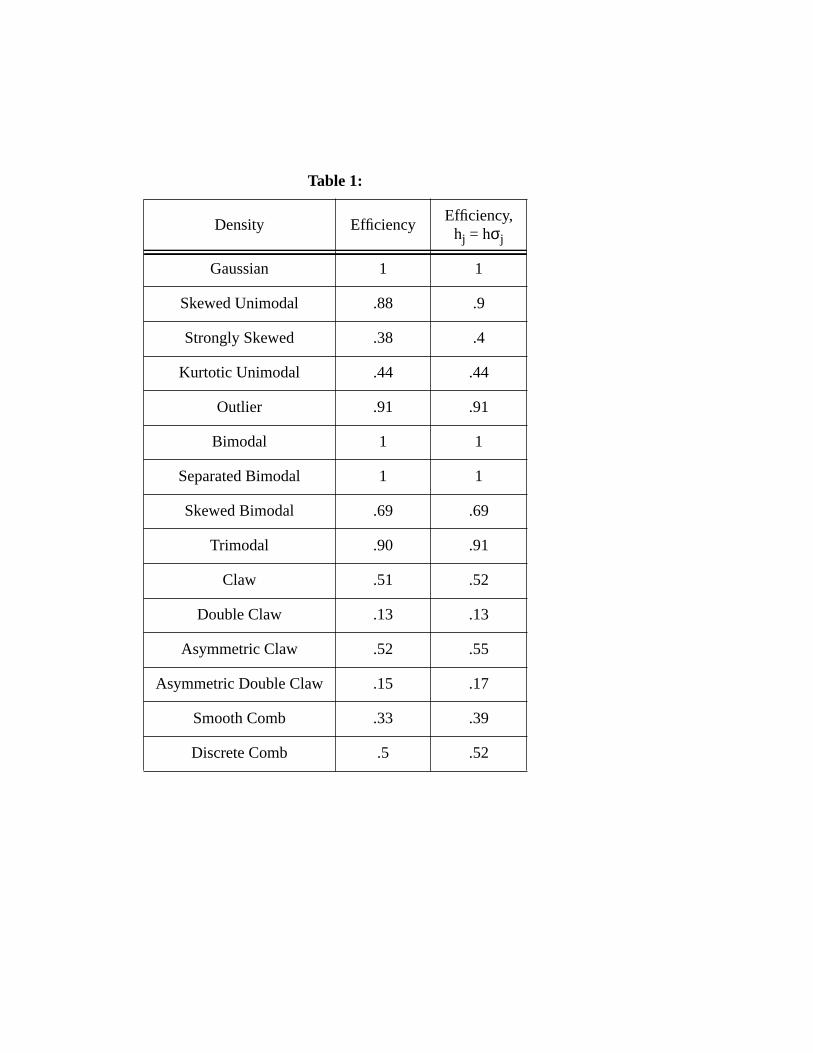
Table 1:

Density EfficiencyEfficiency,

hj = hσj

Gaussian 1 1

Skewed Unimodal .88 .9

Strongly Skewed .38 .4

Kurtotic Unimodal .44 .44

Outlier .91 .91

Bimodal 1 1

Separated Bimodal 1 1

Skewed Bimodal .69 .69

Trimodal .90 .91

Claw .51 .52

Double Claw .13 .13

Asymmetric Claw .52 .55

Asymmetric Double Claw .15 .17

Smooth Comb .33 .39

Discrete Comb .5 .52

-5 0 5 10 15 20

0.0

0.2

0.4

0.6

0.8

1.0

-5 0 5 10 15 20

0.0

0.2

0.4

0.6

0.8

1.0

Figure 1

An example of the filtered kernel estimator applied to the two component

mixture 0.3N(-2,1) + 0.7N(5,50). The mixture probability density function

andρ functions are shown. Example kernels are shown overlaid in (a).

-5 0 5 10 15 20

0.0

0.05

0.10

0.15

-5 0 5 10 15 20

0.0

0.05

0.10

0.15

-5 0 5 10 15 20

0.0

0.05

0.10

0.15

-5 0 5 10 15 20

0.0

0.05

0.10

0.15

-5 0 5 10 15 20

0.0

0.05

0.10

0.15

-5 0 5 10 15 20

0.0

0.05

0.10

0.15

-5 0 5 10 15 20

0.0

0.05

0.10

0.15

(a)

(b)

-2 -1 0 1 2

12

34

-2 -1 0 1 2

12

34

-2 -1 0 1 2

12

34

Effi

cien

cy

-2 -1 0 1 2

0.70

0.75

0.80

0.85

0.90

0.95

1.00

(a)

(b)

Figure 2

(a) Efficiency as a function of log(variance) for Example 1.

(b) The two bandwidths for the FKE are shown as solid lines, with the single

bandwidth of the standard kernel estimator shown as a dotted line.

0 50 100 150 200 250 300

0.0

0.00

20.

004

0.00

60.

008

0.01

00.

012

0 50 100 150 200 250 300

0.0

0.00

20.

004

0.00

60.

008

0.01

00.

012

0 50 100 150 200 250 300

0.0

0.00

20.

004

0.00

60.

008

0.01

00.

012

0 200 400 600 800 1000

0.0

0.00

20.

004

0.00

60.

008

0.01

00.

012

0 200 400 600 800 1000

0.0

0.00

20.

004

0.00

60.

008

0.01

00.

012

0 200 400 600 800 1000

0.0

0.00

20.

004

0.00

60.

008

0.01

00.

012

Figure 3

(a) Two kernel estimators (solid curves) and a 2 component mixture fit to the

hydrocarbon Wiener Index data.

(b) The FKE with “optimal” bandwidths (solid curve) and user chosen band-

widths (dotted curve) and the mixture model (dashed curve) at the mode.

(a)

(b)

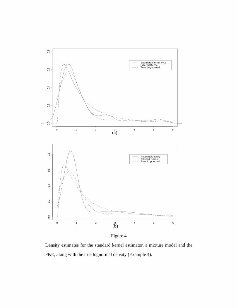
Figure 4

Density estimates for the standard kernel estimator, a mixture model and the

FKE, along with the true lognormal density (Example 4).

Lognormal Data

Den

sity

Est

imat

e

0 1 2 3 4 5 6

0.0

0.2

0.4

0.6

0.8

Standard Kernel h=.3Filtered KernelTrue Lognormal

Lognormal Data

Den

sity

Est

imat

e

0 1 2 3 4 5 6

0.0

0.2

0.4

0.6

0.8

Filtering MixtureFiltered KernelTrue Lognormal

(a)

(b)