1

Automatic Request Categorization in Internet Services

Abhishek B. Sharma (USC)Collaborators:

Ranjita Bhagwan (MSR, India)Monojit Choudhury (MSR, India)

Leana Golubchik (USC)Ramesh Govindan (USC)

Geoffrey M. Voelker (UCSD)

2

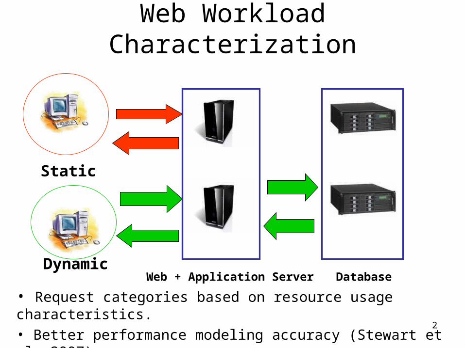
Web Workload Characterization

Static

DynamicWeb + Application Server Database

• Request categories based on resource usage characteristics.

• Better performance modeling accuracy (Stewart et al. 2007).

3

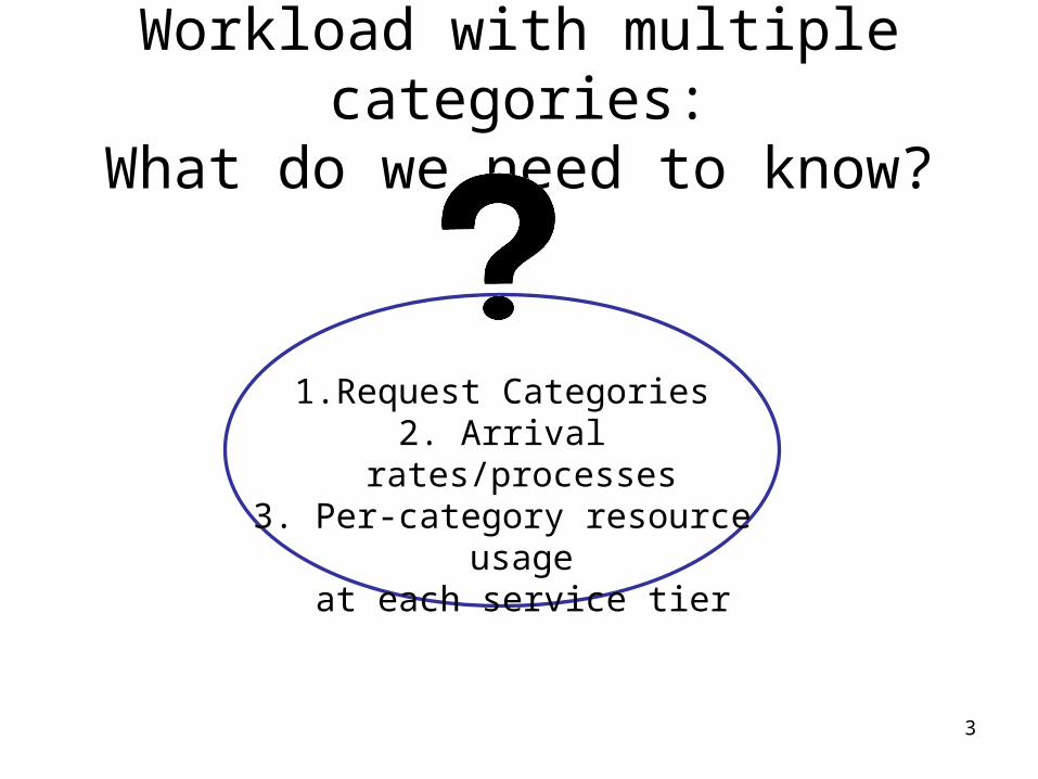
Workload with multiple categories:What do we need to know?

1. Request Categories2. Arrival rates/processes

3. Per-category resource usage at each service tier

4

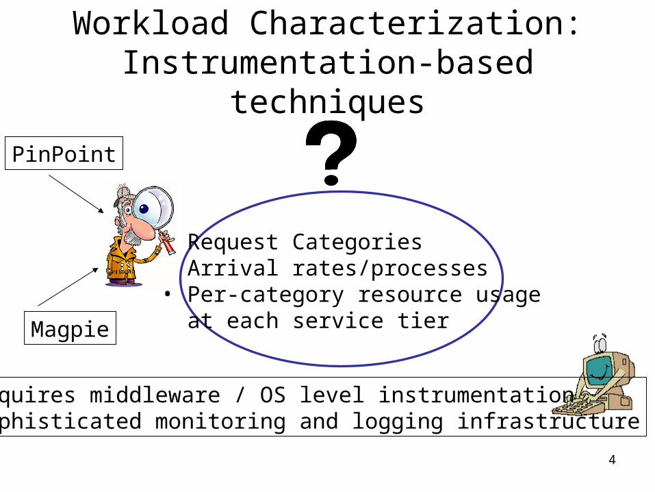
Workload Characterization:Instrumentation-based techniques

• Request Categories• Arrival rates/processes• Per-category resource usage at each service tier

PinPoint

Magpie

• Requires middleware / OS level instrumentation • Sophisticated monitoring and logging infrastructure

5

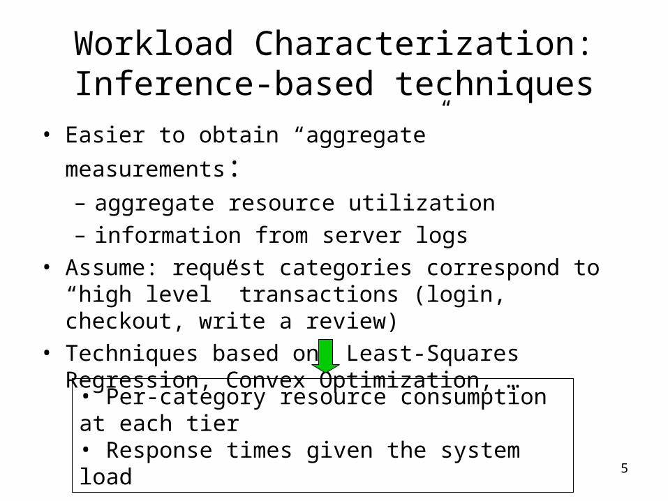
Workload Characterization:Inference-based techniques

• Easier to obtain “aggregate” measurements: – aggregate resource utilization– information from server logs

• Assume: request categories correspond to “high level” transactions (login, checkout, write a review)

• Techniques based on: Least-Squares Regression, Convex Optimization, …

• Per-category resource consumption at each tier• Response times given the system load

6

“Hot” Question ?

• Is there an inference technique that does not assume knowledge of the request categories?

• If yes, then– do not need invasive instrumentation– can infer the request categories and the workload

mix.– can infer the service times (resource consumptions)

for each request category

7

Our Approach

• Two key elements.• A linear model for aggregate resource

consumption.

• Use Blind Source Separation methods to infer

the request categories and their resource consumption characteristics.

8

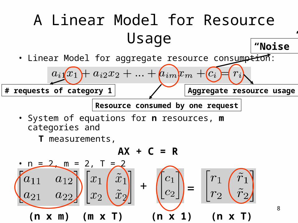
A Linear Model for Resource Usage

• Linear Model for aggregate resource consumption:

• System of equations for n resources, m categories and T measurements,

AX + C = R• n = 2, m = 2, T = 2

Aggregate resource usage# requests of category 1

Resource consumed by one request

+ =

(n x m) (m x T) (n x 1) (n x T)

“Noise”

9

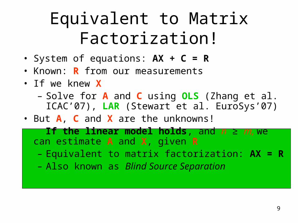
• System of equations: AX + C = R• Known: R from our measurements• If we knew X

– Solve for A and C using OLS (Zhang et al. ICAC’07), LAR (Stewart et al. EuroSys’07)

• But A, C and X are the unknowns! If the linear model holds, and n ≥ m, we can estimate A

and X, given R– Equivalent to matrix factorization: AX = R– Also known as Blind Source Separation

Equivalent to Matrix Factorization!

10

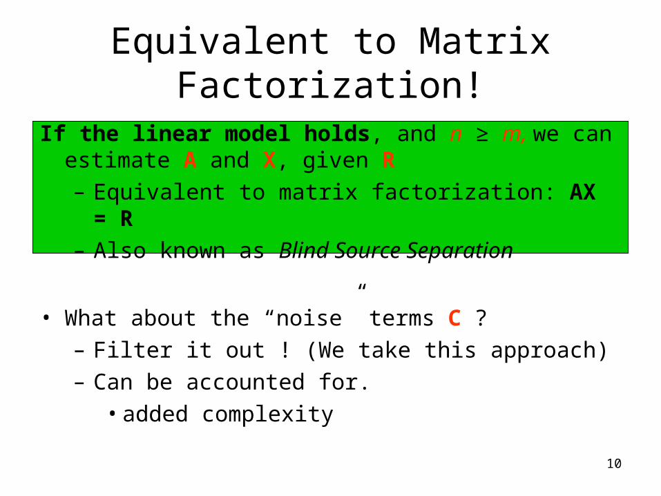
Equivalent to Matrix Factorization!

If the linear model holds, and n ≥ m, we can estimate A and X, given R– Equivalent to matrix factorization: AX = R– Also known as Blind Source Separation

• What about the “noise” terms C ?– Filter it out ! (We take this approach)– Can be accounted for.

• added complexity

11

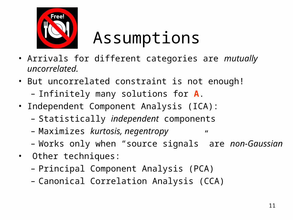
Assumptions

• Arrivals for different categories are mutually uncorrelated.• But uncorrelated constraint is not enough!

– Infinitely many solutions for A.• Independent Component Analysis (ICA):

– Statistically independent components – Maximizes kurtosis, negentropy – Works only when “source signals” are non-Gaussian

• Other techniques:– Principal Component Analysis (PCA)– Canonical Correlation Analysis (CCA)

12

Methodology

• We use ICA.– FastICA package (Thank you, Hyvarinen !)

• PCA used to pre-process R.• Evaluation: E-commerce workload

– An online store: “Browsing” and “Shopping” sessions– Tools: Microsoft PetShop 4.0 – Visual Studio Test Suite (for Client Emulation)

• Testbed:– Microsoft IIS 6.0 (web server)– Microsoft SQL Server 2005 (database)

13

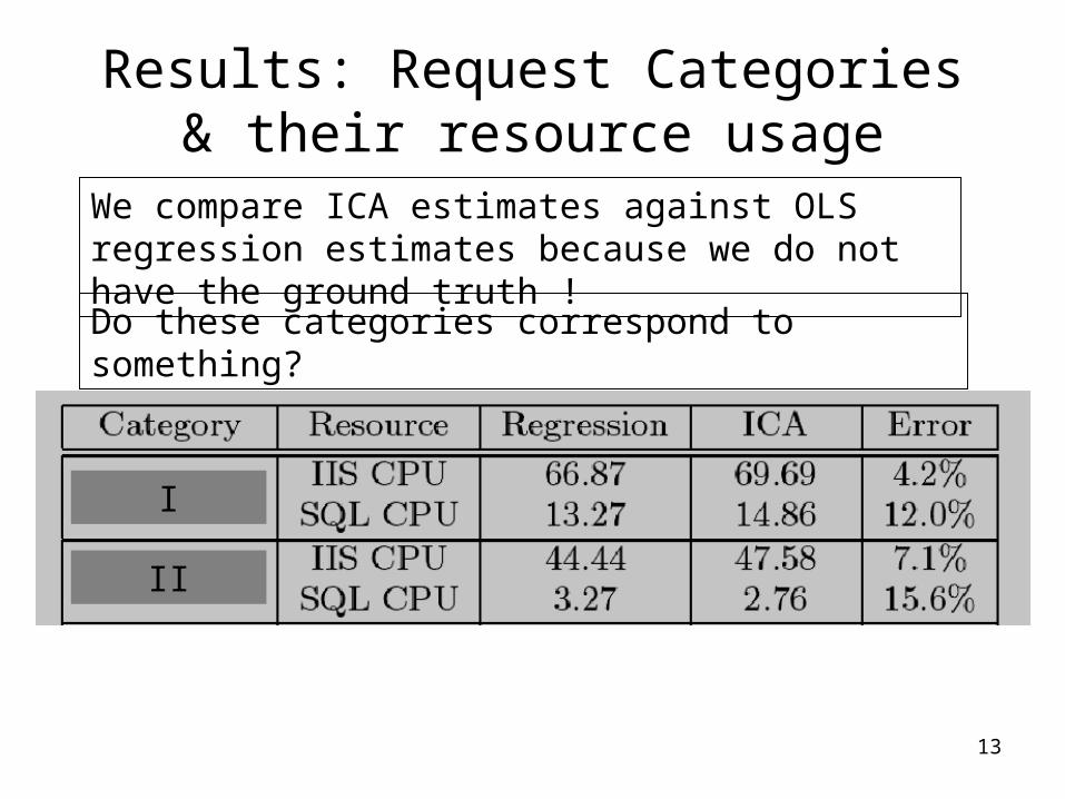
Results: Request Categories& their resource usage

We compare ICA estimates against OLS regression estimates because we do not have the ground truth !

I

II

Do these categories correspond to something?

14

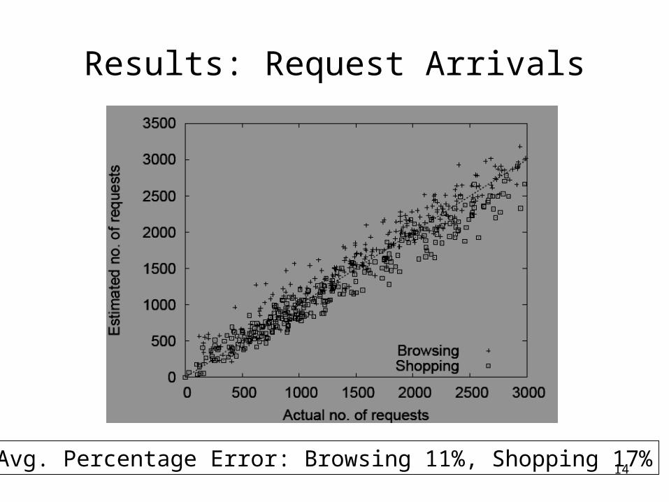
Results: Request Arrivals

Avg. Percentage Error: Browsing 11%, Shopping 17%

15

Is the Linear Model valid?

• At best, approximate fit

• Conjecture: Not valid when– Heavily load

• Does not capture?– Interaction effects across requests.– Autocorrelation in resource consumption.– More severe in heavily loaded system

• Stewart et al. (Eurosys’07), • Mi et al. (Performance’07)

16

What about the ICA assumptions?

1. ICA assumes non-Gaussianity and Independence.

2. All BSS methods assumes mutually uncorrelated “sources”

non-Gaussianity: – Per-second aggregate arrivals are non-Gaussian – Sampling interval should not be too large (~ 10 min)

Independence/mutually uncorrelated:– May not always hold.– In practice, FastICA finds as independent

components as possible.

17

Future Work1. Determining m, the number of categories ?2. Effect of noise

– FastICA is known to be robust against noise. – “Noisy” ICA

3. Which request belongs to which category?– Goldszmidt et al. (EC’01)

4. How do results from CCA compare against ICA?– “Autocorrelated” constraint might be less restrictive

than “independence” constraint in the real world.5. Evaluation using benchmarks—TPC-W, RuBiS, real

system traces.6. Use queueing network models to tie our workload

characterization work with end user quality of service.

18

Thank you