^ the roscoe manual - apps.dtic.mil · cd n ^ the roscoe manual 01 volume be - systems models c...
TRANSCRIPT

CD N
^ THE ROSCOE MANUAL
01 Volume BE - Systems Models C
Oeneral Research Corporation
^ P.O. Box 3587
Santa Barbara. California 93106
October 1975
^
DNA 3964F-4
Final Report for Period 1 March 1074—30 September 1975
^ CONTRACT No. DNA 001-74-C-0182
APPROVED FOR PURLIC RELEASE; DISTRIBUTION UNLIMITED.
k THIS WORK SPONSORED BY THE DEFENSE NUCLEAR AGENCY UNDER RDT&E RMSS CODES B322074464 S99QAXHC06428 H2590D AND B322075464 S99QAXHC06432 H2590D.
Prepared for
Director
DEFENSE NUCLEAR A6ENCY
Washington. D. C. 20305

Destroy this report when It is no longer needed. Do not return to sender.
0N,

UNCLASSIFIED FICATlON Or THIS PACE (*h*n Dm» Bnltfd)
m
REPORT DOCUMENTATION PAGE I, OOVT »CCES:
f ritiiiin
JHE jOSCOE 2JANUAL. "Volume IV, -^-Systems Model« /
H. S./ostrowsky^ / P. J.Aedaond I [l^\ J. R.^Garbarlno^ ^ R. E.Aein / ( /O J
*cn*omiiiR INIIATION NAME AND AOONKSt
General Research Corporation P. 0. Box 3587 Santa Barbara, California 93105
n. CONTNOLLIHO orncc NAME AND AOONCSS
Director Defense Nuclear Agency Washington, D.C. 20305
I«. MONITOHINC AOCNCV NAME ' ' • Aoo«EsSrtÄBPfiiw^SSitSiifT"^:7r
CR-l-520, Volume I CONTBACT O« GRANT NUMBtRfx
DN/yj^i -74-0^182 /
10 PROGRAM ELEMENT PROJECT, TASK ARE* • WORK UNIT NUMBERS
NWED Subtask S99QAXHC064-28-32
216 IS SECURITY CLASS fo( ihn r«por/;
UNCLASSIFIED
ISa. DECL ASSlFICATlON DOWNGRADING SCHEDULE
I«. DISTRIBUTION STATEMENT fol Ala Mapwt;
Approved for public release; distribution unlimited.
»r«c< wtlwwt I« Blot* 20, H <fl/faranl Ifoai Rtpjfl)
ci-d-sw-yoi' \%. SUPPLEMENTARY NOTES
This work sponsored by the Defense Nuclear Agency under RDT&E RMSS Codes B322074464 S99QAXHC06428 H2590D and B322075464 S99QAXHC06432 H2S90D.
K. KEY WORDS fConflnua an rayar«» attfa II nacaaaarr and Htntlty by block number I
Nuclear Effects Badar Optical Sensors Computer Program
Simulation Ballistic Missile Defense
20. ABSTRACT (Continum an ravaraa alrfa /I nacaaaary and Idmllly by block number)
The RGSCGE computer code is designed specifically to be the "laboratory standard" for evaluating nuclear effects on radar systems. The program provides a means for (1) evaluating radar acquisition, discrimination, and tracking performance in a nuclear environment, (2) measuring various pro- pagation error sources, and (3) computing specific phenomenological data.
(Continued)
DO I JAN 71 1473 EDITION Of I NOV •> IS ODSOLETE UNCLASSIFIED SECURITY CLASSIFICATION OF THIS PAGE (When Dml. a Entered) f

■n»
UNCLASSIFIED tccuniTv CLMtiricATioM or THIS PAOKr"*«» o*
20. ABSTRACT (Continued)
The R0SC0E users manual Is divided Into four volumes:
Volume I: Volume II: Volume III: Volume IV:
Program Description Sample Cases Program Structure Systems Models
Volume I provides the user with a brief overview of the code, a description of the Input and output, and some sample Input decks. Volume II contains Illustrative examples showing the use of the code In various modes. Volume III presents structural details of the code (such as the subroutine structure and dataset structure) for the programmer-user. Volume IV describes the systems content of the code.
•
MCBSINUr
lilt Vft'tt St' NC m Sect!« Q
MtHOMKI u «KIlFtUTIM «C
IT ittniUTiN/miuiiiiTi ma
TB m\L m/w 9u
A UNCIASSIFIED
SECURITY CLASSIFICATION OF THIS PAGErtfh.n D«l* F.nltttdj

CONTENTS
SECTION PAGE
1 INTRODUCTION 9
2 MISCELLANEOUS MODELS 11
2.1 Attack Generator and Object Motion U
2.2 Object Observables 14
2.2.1 Ballistic Coefficient 14
2.2.2 Tumbling 16
2.2.3 Radar Cross Section 18
2.3 Sensor Platforms 20
2.4 Track Filter 20
3 RADAR EVENT LOGIC 27
3.1 Search/Detection/Verification Events 27
3.1.1 Assumptions 27
3.1.2 Procedures 29
3.1.3 Flow Charts 31
3.2 Track Initiation Event 35
3.2.1 Assumptions 35
3.2.2 Procedure 37
3.2.3 Details 40
3.2.4 Flow Charts 46
3.3 Track Event 46
3.3.1 Assumptions 46
3.3.2 Procedure 52
3.3.3 Definitions 54
3.3.4 Inputs 55
3.3.5 Outputs 56
3.3.6 Logical Outline of the Flow Charts 57

CONTENTS (Cont.)
SECTION
3.4 Discrimination Event
3.4.1 Astumptions
3.4.2 Procedure
3.4.3 Fine-Frequency Length Model
3.4.4 Wide-Bandwidth Length Model
3.4.5 Flow Diagrams
RADAR SIGNAL PROCESSING
4.1 Overall Structure
4.2 Possible Targets List
H.2.1 Subroutine POSSV
4.2.2 Subroutine POSLIST
4.2.3 List POSLST
4.3 Environmental Effects
4.3.1 Subroutine RAD1S
4.3.2 Subroutine REF1S
4.3.3 Subroutine DISPERS
4.4 Revised Target List
4.4.1 Subroutine REFLST1
4.4.2 Subroutine GOA
4.4.3 Subroutine REFLSTN
4.4.4 Subroutine MULTOAR
4.4.5 LISTA and LISTS
4.5 Target Position and Signal-to-Noise-Plus-Clutter Ratio
4.5.1 Subroutine TARGS1
4.5.2 Subroutine TARGM1S
4.5.3 Subroutine TARGMSV
4.5.4 Subroutine TARGMTS
PAGE
61
61
62
63
65
66
69
69
74
74
76
76
78
78
82
88
90
90
92
93
95
95
98
98
100
100
100

CONTENTS (Cont.)
SECTION
4.6 Subroutines Called by Target-Position Subroutines
4.6.1 Subroutine MN0PLS1
4.6.2 Subroutine MNOPLS
4.6.3 Subroutine MNOPLSM
4.6.4 Subroutine SPLTGAT
4.6.5 Subroutine MLTSPLT
4.6.6 Subroutine SVPEAKS
4.6.7 Subroutine SLNINT
4.6.8 Subroutine SLNINTM
4.6.9 Function AMBGN(X)
4.6.10 Function QINV(8)
4.7 Thresholding and Radar Measurement Errors
4.7.1 Subroutine MEASERR
4.7.2 Subroutine XTHRSHS
PROPAGATION
5.1 Absorption
5.1.1 Assumptions
5.1.2 Procedure
5.1.3 Flow Charts
5.1.4 Inputs and Outputs
5.2 Fireball Noise
5.2.1 Assumptions
5.2.2 Procedure
5.2.3 Flow Chart
5.2.4 Inputs and Outputs
5.3 Refraction
5.3.1 Gross Refraction
5.3.2 Refraction Due to Strlatlons
5.3.3 Procedure
5.3.4 Flow Chart
5.3.5 Inputs and Outputs
PAGE
104
104
106
106
106
110
110
113
113
116
116
119
119
122
124
124
124
125
126
127
130
131
132
133
136
137
13?
138
139
139
142

SECTION
APPENDIX A
APPENDIX B
APPENDIX C
APPENDIX D
APPENDIX E
APPENDIX F
APPENDIX G
CONTENTS (Cont.)
5.A Clutter
5.4.1 Assumptions
5.4.2 Procedure
5.4.3 Flow Charts
5.4.4 Inputs and Outputs
5.5 Low-Altitude Multipath
5.5.1 Assumptions
5.5.2 Discussion
5.5.3 Inputs and Outputs
REFERENCES
COORDINATE SYSTEMS IN ROSCOE
DISPERSION AND THE RADAR AMBIGUITY FUNCTION
MONOPULSE
THE SPLIT-GATE RANGE TRACKER
THE SPREAD TARGET CLOUD IN THE RADAR BEAM
STOCHASTIC REFRACTION MODEL
DEFINITIONS OF SYMBOLS
PAGE
1^3
1U3
Ihk
1U6
1U9
IU9
1U9
151
155
157
159
165
171
177
181
189
205
•
J

«MMMMK ':
ILLUSTRATIONS
FIGURE NO. PAGE
2.1 Program ATKGEN 13
2.2 Function BETAGT 15
2.3 Subroutine TUMBLR 17
2.4 Function RCSMODL 19
2.5 Subroutine FILTER 22
3.1 Vertical Slice Through Search Sector with Range-Height 28
Transition
3.2 Search Initialization Flow Chart 33
3.3 Search Flow Chart 34
3.4 Verification Flow Chart 36
3.5 Track Initiation (Til Pulses) Flow Chart *7
3.6 Track Initiation (TI2 Pulses) Flow Chart 48
3.7 Track Flow Chart 58
3.8 Discrimination Flow Chart 6*
3.9 Fine-Frequency Length Discrimination Flow Chart ^7
3.10 Wlde-Baudwldth Length Discrimination Flow Chart 68
4.1 Radar Signal Processing Subroutine Hierarchy 70
4.2 Subroutine RADMODS 72
4.3 Subroutine POSSV 75
4.4 Subroutine POSLIST 77
4.5 Subroutine RAD1S 79
4.6 Subroutine REF1S 83
4.7 Subroutine DISPERS 89

ILLUSTRATIONS (Cont.)
I FIGURE NO.
4.8 Subroutine REFLST1
4.9 Subroutine GOA
4.10 Subroutine REFLSTN
4.11 Subroutine MULTOAR
4.12 Subroutine TARGS1
4.13 Subroutine TARGM1S
4.14 Subroutine TARGHSV
4.15 Subroutine TARGMTS
4.16 Subroutine MN0PLS1
4.17 Subroutine MNOPLS
4.18 Subroutine MNOPLSM
4.19 Subroutine SPLTGAT
4.20 Subroutine MLTSPLT
4.21 Subroutine SVPEAKS
4.22 Subroutine SLNINT
4.23 Subroutine SLNINTM
4.24 Function AMBGN
4.25 Function QINV
4.26 Subroutine MEASERR
4.27 Subroutine XTHRSHS
5.1 Subroutine ABSORB
5.2 Subroutine FBABS
5.3 Subroutine DELABS
PAGE
91
93
94
96
99
101
102
103
105
107
108
109
111
112
114
115
117
118
120
123
127
128
129

ILLUSTRATIONS (Cont.)
FIGURE NO.
5.4 Fireball Noise Integration Procedure
5.5 Subroutine NOISE
5.6 Ray Trace Procedure
5.7 Subroutine REFRCT
5.8 Subroutine FBCLTR
5.9 Subroutine CLUTRFB
5.10 Specular Reflection Point
5.11 Subroutine MLTPATH
5.12 Subroutine BOUNCE
5.13 Bounce Path Geometry
PAGE
132
134
140
141
147
148
151
152
153
154
■ J

1 L INTRODUCTION
This volume describes the systems content of the ROSCOE code. The
systems model, as defined here, consists of these major blocks: attack
generation, object observables, sensor platforms, track filter, radar
event logic, radar signal processing, and radar propagation.
The objective in building the systems model was to provide a very
generalized set of routines which could be used by a variety of users for
a variety of applications, kv a result, the user can select from among a
number of options to simulate a particular engagement. For example, any
number of different object types, radar types, and weapon types can be
specified in a single run. In addition, launch and impact points can be
mixed to generate complex attacks, A Section 2 of this volume briefly describes the ROSCOE models of at-
tte^k generation and object motion, object radar observables, sensor plat-
forms, and radar track filter. References are given for fuller descriptions.
Section 3 describes the radar logic in terms of the radar "events":
search/detect/verify, track initiation, track, and discrimination. Assump-
tions are explicitly identified; procedures are described in detail; and
annotated flow charts are presented.
Section 4 describes the ROSCOE models of the signal processing that
is applied to each radar pulse (radar look event). These models account
for the effects of the environment (by calling the propagation routines.
Sec. 5) and of radar characteristics such as monopulse processing, range
gating, and signal design (ambiguity function).
Section 5 describes the radar propagation models. These models link
the systems part of ROSCOE with the environment p'rt by calculating the
effects on radar signals of absorption, fireball noise, refraction, clutter,
and multipath.

Appendixes supply the background for some of the signal processing
algorithms.
10

MISCELLANEOUS MODELS
:
2.1 ATTACK GENERATOR AND OBJECT MOTION
The attack generator for ROSCOE Is taken from General Research Cor-
poration's BAG 14 code. It consists of the following set of programs:
ATKGEN
LAUNCH
PHIMP
Attack generation program
Creates objects and object position arrays
Creates burst arrays at Impact
The programs use the following subroutines to generate the object trajec-
tories ard find specific points on them:
0RB2
0RB1
ORB?
BLLSTIC
DR0RB2
GENORB
ADVANCE
KUTTA
PREDLOC
WHERE
Determines the elements of a Keplerlan orbit
joining two points
Determines the orbital elements corresponding
to a given state
Determines the state vector of a point on a
Keplerlan orbit
Generates an endo-atmospherlc trajectory with
slowdown
De-orbit routine which modifies an orbit to
meet a specified Impact point
Corrects an orbit to meet a specified impact time
Advances the state and covariance of an object
to the current time
Trajectory integration routine
Returns a predicted object location
Finds object state at a specified time
* 2 These routines are part of the General Research Corporation TRAID system.
11
Figure 2.1 Is a flow diagram of the main program In this module
(ATKGEN). The Input consists of a set of launch points (dataset LP) and
a set of target points (dataset TG) specified by the user. These datasets
may have repeated entries and may be In quite arbitrary order. The attack
generator takes each target point In order. Associated with the target
point as an Input Is the number of reentry objects which the target point
Is to receive. This number of objects Is assigned to the target point
one at a time by a sequential pass through the list of launch points. If
the end of the list Is reached before all the target points are satisfied,
the program cycles back to the front of the list of launch points and con-
tinues. Thus, In a simple attack with a single launch point, one entry
on the list Is sufficient. It should be noted parenthetically that object
type Is peculiar to launch point; thus to mix RVs and decoys requires
mixing launch points on the launch point list.
The timing of the attack and the type of trajectory are specified
with the target point (dataset TG). These data Include the desired arrival
time for the first booster, the desired time separation between objects,
the slgma of arrival time errors, and the CEP of position errors. An
alternative form of timing specification allows the user to specify a
fixed time interval Inside which the reentry objects assigned to a
particular target point arrive in random order.
2 The trajectory is specified as in TRAID and is calculated with drag
on a round, rotating earth. For each reentry object, the attack generator
generates a launch event at the time at which the Keplerian position of
the orbit leaves the launch point. The storage for each object will be
set aside when the launch event Is processed—all that is saved during
the attack generation is the computed orbital elements, which are appended
to the launch event.
The launch event creates an object and names it. (The object
LP-5 7 is the seventh launch from the launch point called LP-5.) Object
and object position arrays are created. Orbital element and reentry
12 1

( ST0P > INTERVAL
ATTACK
i
UN IF MM ATTACK
GET FIRST TARGET POINT AND LAUNCH POINT
CREATE LAUNCH EVENT DATASET
CREATE POINTERS TO LAUNCH POINT AND TARGET POINT DATA- SETS
COMPUTE RANDOM CROSS RANGE AND OOHNMNGE IMPACT ERRORS AND TIME AT IMPACT
DETERMINE CURRENT INDEX FOR BOOSTER TYPE AND BETA DATASETS
CALL GENORB (GENERATES TRAJECTORY)
INSERT EVENT IN EVENT LIST ORDERED BY TIME
UNLOCK LAUNCH EVENT DATASET H0
Figure 2.1. Program ATKGEN
13

position state vectors are constructed, as Is a summary output array for
that object. Future events associated with the object are constructed
and placed on the event list. These are
• The impact event (Program PHIMP)
• A potential acquisition event (Program RADAR) for each
radar in the defense system
The impact event is created at the same time the object is created
and occurs at the moment that the object trajectory passes through its
designated target point. In particular, this means that if an airburst
(or a precursor) is desired, the target point should be specified at a
non-zero altitude.
2.2 OBJECT OBSERVABLES
This section describes the following object observables models:
1. Ballistic coefficient
2. Tumbling dynamics
3. Radar cross section
3 The models are taken from General Research Corporation's SETS model.
In the following sections, flow diagrams are shown for each routine
with explanatory notes to define the variables and describe the computations.
2.2.1 Ballistic Coefficient
The ballistic coefficient (beta) is found by calling Function BETAGT
(Fig. 2.2) with the object state and a dataset pointer (DSP) to the bal-
listic coefficient model type desired. There are three model types: type 1
uses a constant value of beta for all altitudes; type 2 uses an N-point
altitude-beta table, resulting in a piecewise-linear relation between beta
and altitude; and type 3 relates the beta history of an object to the
dynamics of a theoretical conical vehicle of constant mass and shape.
Ik

BETA » CONSTANT
C RETURN j
r BETA • MINB (MINIK'JM BETA)
DO TABLE INTERPOLATION FOR BETA AT THIS ALTITUDE
-~f RETURN J
COMPUTE MACH NO.: M = M
COMPUTE cw
COMPUTE c.
.3125 ♦\M^ 1 sin e
0.0625 + YM^lsin ec
c 1
?
OTHERWISE
COMPUTE cw
Cx.Zs1n 6C 1. + / 0.3125 + 1.
( Ö.0625 ♦ r 118 sin 6
118 sin e c !.♦& 44444 \ <M-0-
$1n29, /
5)
COMPUTE NOMINAL BETA:
BETA • ^
SELECT RANDOM NUMBER R FROM G (0. SIG B)
• BETA • BETA ♦ R
Tgcr f RETURN J
Figure 2.2. Function BETAGT
15

In type 2, the altitude-beta pairs are given In order of decreasing
altitude. For object altitudes above the first In the list, the beta
value for the highest altitude Is used. For object altitudes below the
last In the list, the last beta value Is used.
In type 3, the quantities shown In Fig. 2.2 are defined as follows:
m ■ mass of vehicle, lb
2 A ■ aerodynamic reference area, ft
c B axial drag coefficient
6 - theoretical cone angle, deg
M » nach number
c = local speed of sound, m/s
v ■ current vehicle velocity, m/a
At altitudes above 150 km, type 3 uses an Input minimum beta, with no
further computation required.
The ballistic coefficient computed by model type 3 may be randomized
by adding a number drawn from a Gaussian distribution G(0, SIGB) with
zero mean and an input standard deviation SIGB.
2.2.2 Tumbling
The tumbling model (Subroutine TUMBLR, Fig. 2.3) is called with the
object state vector and a DSP word denoting the model type, and returns
a vector (AVEC) describing the motion of the object about its point mass
trajectory.
There are three tumbling models available. They all assume that
the object is a solid of revolution with one axis of rotational symmetry
(body axis). It is assumed that the cone swept out by the tumbling body
axis differs negligibly from a plane (tumble plane). Type I keeps the
object oriented along its current velocity vector; therefore, no data is
16

c RETURN > AVEC
AVEC
a - TRÄTE • (T-TINIT)
h = E
u * u
sin o 0 sin «f,
cos » 0 cos e.
AVEC » F ♦ u IF* ül
SELECT 3 RANDOM VECTOR COMPONENTS FROM: U (0,1)
AVEC •T7T
i
TURN ^ RETURN
NORMALIZED RESULTANT 3 VECTOR • TAXIS
SELECT TWO RANDOM VECTOR COMPONENTS FROM: U (0.1)
v D * ^z"- fAXIS
I'«-1 rAxisi
v R2*
TAXIS
1 TAXIS
tan"1 !M w AVEC ■k
+ iro + uol
f RETURN J
Figure 2.3. Subroutine TUMBLE
17

required for this model. Type 2 orients the body along its initial reentry
velocity vector (computed at 100 km, or at the object's current altitude
if the initial call occurs below 100 km). Type 3 is a stochastic model
which allows an object to tumble at a given rate until its body axis sta-
bilizes along the velocity vector at a given (input) stabilization altitude.
The initial body orientation and tumble plane are derived as follows:
1. Three random components are chosen from a uniform random
distribution.
2. A three-vector formed by normalizing these, components
defines a tumble axis (TAXIS).
3. A tumble plane normal to this axis is formed and a random
vector in the plane chosen by selecting two more random
numbers from the uniform distribution. This latter vector
is called the body axis (AVEO.
4. After initialization, the body axis is updated by using
the input tumble rate and the definition of the tumble
plane (ho,uo).
2.2.3 Radar Cross Section
Four models are available for modeling an object's RCS (Function
RCSMODL, Fig. 2.4). Type 1 assumes the RCS is constant and requires no
other input data. The other three models compute RCS as a function of
the aspect angle (defined as the angle between the radar line-of-sight
and the current orientation of the body axis as given by the tumbling
model).
In the type 2 model, the RCS is found by interpolation of an RCS
vs aspect angle table. Type 3 is intended for tank-like objects (cylinders),
while type 4 is for RVs and decoys.
18
—

mmm
/REQUEST: ^OBJECT DATASEy
c
RCS ■ CONSTANT
RETURN 3
CALL TUMBLE SUBROUTINE FOR BAXIS
1 COMPUTE ASPECT i ANGLE:
rRR = rRV ' rRAD
1 rRR-BAXIS j
♦ - cos IrRRI*I6AX-nT
DO TABLE INTERPOLATION FOR RCS AT THIS ;
DO TABLE INTERPOLATION FOR o AND 3 . (AVERAGE
RCS VALUES) WHICH CORRES- POND TO 4 AND n Vi ASPECT ANGLES
°lw'*» Ico»*| . a|sin »J sin2 (kL cos *)
T k cos t
* Or JEND T 'SIDE + 2 (oEND0SIDE |cos (kL cos <i|-2ka jsln
1/2 )
♦ I)
c RETURN
RCS [ 3n ' Vl u
[1 ♦ B cos Uwt)]
•♦) 1 + A cos (2 kL cos ;)
)
Figure 2.4. Function RCSMODL
19

In Fig. 2.4, the variables used In type 3 are defined as follows:
a - radius of tank, m
L - length of tank, m
i ■ aspect angle, deg
k - 2IT/\
A - wavelength, m
and the variables used In type 4 are defined as follows:
w « spin rate, rad/s
a - number of RCS peaks per revolution
A,B ■ constants for vehicle In question, as used In the
equation shown In Fig. 2.4
2.3 SENSOR PLATFORMS
Three sensor platform models are currently available In ROSCOE: fixed,
orbital, and circular-orbit. They are specified by placing the proper
dataset (PI, P2, or P3, respectively) in the input deck. The platform
(radar) location is found by calling subroutine PLTFRM with a pointer to
the dataset containing the platform position information. The routine
returns the position through the calling sequence.
The "fixed" platform is simply described by a position vector. The
"orbital" platform is described by a TRAID ten-vector giving its orbital
elements. The "circular-orbit" platform is described by a simplified set
of orbital elements defining a circular orbit.
2.4 TRACK FILTER
The GRC BAG 14 tracking filter has been suitably modified for use
in ROSCOE. It is a fully coupled seven-state Kaiman filter with an option
for exponential memory decay.
20

■MM
The filter module Is made up of five subroutines:
FILTER Initializes covarlance and updates filter
predictions (Fig. 2.5)
CHOLSKI
JACOBIAN
XFORM
KALMAN
Inverts an N ' N matrix
Sets up Jacoblan matrix for filter routine
Inverts Gamma matrix to Covarlance and vice versa
Kaiman filter
The formulation of the tracking filter, expressed In radar face
coordinates, Is as follows. If we define the three-dimensional vector
x by
x.. ■ r sin a
x2 ■ r sin B
x- ■ r(l - sin a - sin 0)
where r, a, 6 are range and radar angular coordinates, respectively,
then the seven-dimensional state vector estimated by '-he filter Is given by
X - (x,xA,X)
where A Is the time between pulses for a given track file and X Is
the natural logarithm of the ballistic coefficient. The equations of
motion giving the time history -if X are assumed to be
-PgW -X .
xx - GMR , +üJ*X + UX (mxR)
J e
(2.1) R ■ x + R
X - w(t)
21

ACCESS DATASETS: |
1 IF FIRST TIME THROUGH: MIDDLE ■ 1 KFLAG = 0
RETURN INDEX TO FILTER PARAMETER DATASET (TF)
RUNNING ENTRY POINT FOR NEW MEASUREMENTS
RETURN INDEX OF TRACK FILTER DATASET (TK)
ADVANCE STATE AND COVARIANCE TO TIME OF THIS EVENT
CÄLrÄDVANCE- ~
_ i SET PREDICTED MEASUREMENTS
I MIDDLE • 2
C RETURN j
INITIALIZE FILTER IN THIS SECTION
CREATE TRACK FILTER DATASET (TK) OF NUMBER TK » 57 WORDS
RETURN DSP WORD FOR TRACK FILTER DATASET
INITIALIZE COVARIANCE
UNLOCK DATASETS
DO J = 1, M OELMES (J) - YMSAV (J) - YMES (J)
c RETURN
COMPUTE JACOBIAN
MIDDLE ' 3 WORK " 0
MIDDLE • 1 CALL BORDER CALL MATDIAG CALL KALMAN
KFLAG - 1 CALL NLOKDS
(NFILTER) CALL NLOKDS
(NDATA)
(^ RETURN J
Figure 2.5. Subroutine FILTER
22

where R ■ vector from earth's center to radar e
oj ■ earth's angular rotation vector
u ■ stationary, uncorrelated random variable with mean
zero and standard deviation o v
G ■ universal gravitational constant
o ■ atmospheric density
M " mass of earth
This formulation differs from the standard three-degree-of-freedom equation
for reentry motion In that no lift Is considered, and the centripetal acceleration term Is taken as a constant.
The ROSCOE tracking filter Is basically an extended Kaiman filter
and, as such, gives a running estimate of the error covarlance matrix C
associated with X . The filter can be separated Into three distinct
operations—Initiation, prediction, and correction—of which only the
last two are repetitive. To distinguish the estimates of the state vector
and covarlance matrix resulting from the prediction and correction steps,
they are given the subscript p or c , respectively.
The filter can be Initiated either through the track initiation logic
or through handover from another radar. In both cases, it is assumed
that the first six components of X are given at the time of the first
tracking pulse, along with some estimate of variance and covarlance between
them. The initial estimate of X is currently £n(100 lb/ft2) - 4.605 ,
and the initial variance is equal to 4. The covariances between X and
the remaining components are Initiated as zero.
Having an estimate of X and C at some time t , the filter must
be able to predict the best estimate of these quantities at some future
time, usually to determine the radar gating and beam pointing for the next
23

pulse. The prediction step Is always carried out over one cycle time -►
A . The subvectors of X are predicted by the equations
xp(t+A) - xc(t) + xc(t)A + AL(t)L2/2
• • •• xp(t+A) - xc(t) +xc(t)A > (2.2)
Xp(t+A) - Ac(t)
where x Is evaluated from Eq. 2.1. For the first prediction, the
initial values are used In Eq. 2.2. The covarlance matrix Is predicted
through the use of an approximate transition matrix <Kt+A,t) • The usual
approximation starts with the equations of motion written In the form
X - l(X)
Then the equations are linearized about some nominal value of the state
vector
• • • -,;£ 6X - (X - X ) = — (X )6X - F[X (t)]6X nonr ■+ nom l nomv '
->■ -»■
where X Is usually taken to be the best estimate X . The linearized nom ' c equations then furnish a transition matrix through the matrix formula (to
first order in A):
t+A
(Kt+A,t) - exp J F(t') dt' = I + F(t)A
In the ROSCOE tracking filter, the further approximation Is made in F
that
■+ ■>
9x 9x M o -♦• -►
9x 9x
.
■
2k

so that only the partlals with respect to X contribute to the last four
rows of $ . Once $ is evaluated, C Is predicted through the formula
Cp(t+A) - (Kt A,t)Cc(t)*1(t+A,t) +Q (2.3)
where Q Is a matrix whose only non-zero element Is In the last row and 2 * column and Is equal to a . v
When a measurement Is made, It Is Incorporated Into the estimate
through the correction step. For numerical reasons, a pseudo-observation
vector Y ■ (x,y,r) Is computed from the measured values of r, sin a,
and sin 0 . The single-pulse variance estimates for r, sin a, and
sin ß are computed from the measured slgnal-to-nolse ratio and the pulse
type. If the matrix i^ Is defined as
"sin ot r 0
sin ß 0 r
1 0 0.
then the estimated error covarlance matrix for Y Is computed through the
formula
R - V slna
0
0
0
rsinß_
The 3x7 matrix M Is defined by
M aY^X)
U 8x J
* 2 Currently a Is taken as 0.01A for altitudes les» than 250 kft and v
zero otherwise. The Q matrix keeps the filter memory finite within the atmosphere.
25

Then the correction formulas are given by
Xc(t) - Xp(t) - W[Y(t) - Mxp(t)]
C (t) - C (t) - WMC (t) c p p
W - C MT[MC MT + R]"1 c c
If for some reason no measurement Is available, the filter sets X » X c p and C * C In preparation for the next prediction step.
The use of the Q matrix In Eq. 2 3 keeps the filter memory finite
within the atmosphere and Is employed only below 250 kft altitude. Another
useful technique for decreasing memory length In tracking filters Is
through the multiplication of the covarlance matrix by a "fading factor"
c' - rc r'
where r Is a diagonal matrix having non-zero elements greater than or
equal to one. In the ROSCOE filter, a variation of this approach Is used
wherein the fading factor is applied only to the diagonal elements of
the covarlance matrix. The elements along the diagonal of r are given
by (l,l,l,Y,Y»Yfl) where y " e and T Is a constant which can be
varied with altitude.
26

3 RADAR EVENT LOGIC
The ROSCOE radar model may be divided Into two subsets: radar event
logic and radar signal processing.
The radar event logic Is responsible for setting up and simulating
the search, verification, track initiation, track, and discrimination
events. Each event must contain the logic for selecting the appropriate
signals, transmitting them to the appropriate points, calling for the
correct data processing of any return, deciding (based on the latest
return) what further events are necessary, and finally setting up future
calls for these events at the appropriate time.
This type of event logic is essentially independent of how the radar
signal processing is simulated. The latter therefore constitutes an
independent segment of the radar model, and will be discussed separately
in Sec. 4.
The event logic Is described in the subsections which follow. Each
subsection describes the assumptions which underlie the logic, the process
which Is being modeled, and any limitations of the model. Flow charts
are presented and discussed.
3.1 SEARCH/DETECTION/VERIFICATION EVENTS
3.1.1 Assumptions
During these events, the system is assumed to operate without
monopulse. The target angular position is assumed to be that of the
commanded axis of the receive beam. Many real or proposed radar systems
operate without monopulse in the search mode, so this is a realistic
model.
Bulk filtering, which is a part of the search/verify procedure in
many real radar systems, is not modeled in ROSCOE.
27

It Is assumed that the "real target" Is known and distinguished
from other targets. In particular, when multlpath Is present, only one
of the target Images Is detected by this procedure; the method by which
this target is to be selected Is described later In this discussion. When
real multiple targets are present In the beam(s), the association and
filtering necessary to distinguish the correct new target are not modeled,
but are assumed to be done perfectly. Extraneous targets, whether real
or Images, appear principally In the form of "noise" affecting the return
from the "real" target.
The search sector Is a sector (between specified azimuths) of a
volume of revolution whose vertical cross section has the shape shown in
Fig. 3.1, defined by maximum and minimum ranges, altitudes, and elevation
angles. Note that these quantities cannot all be independently specified;
to prevent a gap at the range/altitude transition, it is required that
MAXIMUM SEARCH ALTITUDE
MAXIMUM SEARCH RANGE
TANGENT RANGE. R
Figure 3.1. Vertical Slice Through Search Sector with Range-Height Transition
28

max. alt. m max. range min. alt. mln. range
The range/altitude transition occurs at an elevation angle
_, . -1 max. alt. E0 - sin 2 max. range
If this angle exceeds the maximum elevation, or if maximum altitude
^maximum range, there is no flat portion of the search sector. Such a
search sector might be used by an area-defense radar; compare, for example,
the radars in the two scenarios specified in the appendixes of Vol. 1
(Search Mode Parameters Dataset). An airborne or orbiting radar might
have a negative minimum elevation angle for search. It should go without
saying that the angular extent of the search sector for any radar face
should lie within the field-of-view specified for that face. In the
program, it is implicitly assumed that this is the case.
If the target appears within the search sectors of more than one
radar face, detection is first attempted by that face for which the target
has the smallest off-boresight angle at the time it crosses the outer
boundary of the search sector.
The time of flight of radar signals is not modeled.
3.1.2 Procedures
The user may elect to make the first try at detection as soon as
the target crosses the outer boundary of the search sector, thus ignoring
the random orientation of the search frame relative to the target position.
Alternatively, he may select the option of modeling this "frame randomiza-
tion" by making the first try at detection at some randomly-selected
instant during the first search frame period after the target crosses
the outer boundary.
29

If the first try at detection falls, succeeding tries are made at
intervals of the search frame time, T , after the first try, until
either a successful detection is made or the target crosses the inner
boundary of the search sector. In the latter case, detection fails to
occur.
The search frame time, T , cannot be chosen completely at random.
It must be short enough, compared with the target velocity and the range
window (AR), so that the radar gets at least two chances at any target
before it crosses the inner boundary. Since the first chance might
(because of frame randomization) occur as much as T after the target
crosses the outer boundary, this means approximately that
2T < AR/V 8 t
where V is the target velocity at the time it crosses the outer bound-
ary. This inequality is not exact and is, in fact, rather conservative;
in many cases, considerably larger values of T would be quite satisfactory. s
When successful detection is accomplished, a verification pulse is
ordered to be transmitted at time T after the successful detection v pulse. The verification pulse uses the same beams and waveform as the
search pulse, but the beam axis is along the commanded position of the
bec-ra axis for the successful search pulse. If the verification return is
above the search-return threshold, verification is assumed to be accom-
plished and track initiation is begun. If the verification is unsuccessful,
search continues at intervals of T after the previous "successful" S
detection.
If the search process were being explicitly modeled, with its raster
scan, it would usually be the case that the target appears somewhere off
the axes of the transmit and receive beams. This is another form of frame
randomization, and It is modeled in ROSCOE by offsetting the axes of the
30

search-mode transmit and receive beams with respect to the target position.
The amount and direction of offset are randomly generated in such a way
Chat the target will be somewhere within the 3 dB beamwidths of these
beams, allowing for refraction.
Refraction. The term "allowing for refraction" is interpreted in
the following ways under the stated conditions:
1. When only one ray path exists. The ray path from the true
target position to the radar is computed. The true azimuth
and elevation at the radar are used for the apparent values
A' and E' ; the apparent range, R' , Is computed with
allowance for both the added length of the curved ray path
and the decreased value of c In plasma.
2. Multiple paths through a single fireball or stria. When
multiple paths are present, one of them will always be the
analytic continuation of the single ray-path occurring at
large distances from the plasma. This ray-path is the
one to use for both outgoing and incoming signals; its
azimuth and elevation at the radar give A' and E' , and
the apparent range along it gives R' ; this Is called the
"apparent position of the true target."
3. Multiple paths through a striated region. In ROSCOE, a
"fuzz-ball" approximation is used (see Sec. 4.3 for further
details), with R*, A', E* being essentially the center of
the apparent target image distribution which is the
"fuzz-ball."
3.1.3 Flow Charts
Definitions. The flow charts refer to several sets of object posi-
tion coordinates. In general, R, A, E refer to range, azimuth, and
elevation with respect to the radar, and R, u, v refer to "sine-space"
coordinates, where u and v are the sines of two orthogonal angles
31

measured from the radar boresight (see Appendix A). These coordinates
are subscripted or primed to Indicate the following:
R' .A1,£' or R*.u'.v' Apparent target coordinates allowing for
refraction but not Including radar measure-
ment errors
R ,u ,v Measured coordinates from search return s' s' s
R ,u ,v Measured coordinates from verification return v v v
(u ,v )T Sine-space coordinates of transmit beam axis
(u ,v )„ Sine-space coordinates of receive beam axis o o R r
Other symbols used In the flow charts are:
6 Angle between llne-of-slght to target and boresight
acU(x,y) Random number chosen from uniform distribution between
x and y
Ii Itlallzatlon (Fig. 3.2). The initialization procedure Is not an
event, but takes place before any actual events have occurred. Its
purpose Is to set up the first search event for each target. An Implicit
assumption Is that search and verification are being performed by the
radar, rather than by some other kind of sensor.
In the Initialization procedure, the time for the first attempt at
detection, t , is computed in vacuum, without reference to refractive
effects. This of course will not give the strictly "correct" time, but
it permits the search events to be time-ordered in advance without calling
upon nuclear-effects and propagation subroutines. The time error Involved
is not likely ever to be significant In the context of program applica-
tions, and the approximation makes it possible to maintain a completely
event-based structure.
Search (Fig. 3.3). The search event Is first set up by the ini-
tialization procedure, and Itself sets up the appropriate succeeding event.
32

f (Pill« J
[iMMAiin AU
f m TI«II j
PROJiCI /Adjü STATE VtCTOS ',0 OüTTR BOUNDAIl» Of S^AtCM SfCIO«. COWJIi t , R, A, [.
0 sn ifAct • o
.
10» ON RADAR FACIS f?
CQHPUTF OfF- BORESIGHT MRU
IFACC • FACE NUHBIR. COMPUTE OFF-SORES IGHT ANGLE, «
SET t • t ■ T 0 0 i
COMPUTE », A, ( OF TARGET AT TIME t
SELECT RANDO' NUHBE«: icU [0.1]
0 0 s
NO OCTECTION FOR THIS TAPGFT
SET UP SEARCH (VIM FOR THIS TAPGfT AT
mmuimi
f RETURN \— END TARGET KiOP,
Figure 3.2. Search Initialization Flow Chart
33
f ENU» J
PROJECT T»»&tT STAU VECTUK 10 TIME t.
CdWUTl S TMGIT *T IKE
[■ Of
«UWING FOR REfkACIION
USING PACE NO. IfACE, COMCUTE SINE-SPACE COOKDINATES, (u'.»'), Of APPARENT TARGET
SELECT RANÜOH NUHBERS: l, bdK-T. 1) COMPUTE AXIS OF TRANSHIT BEAM: u • u ♦ •'«,
v. • v ♦ b'n,
SELECT RANDOM NUMBERS: I, b«U (0, i). COMPUTE i • «■,«, ; ■ 2-b. COMPUTE A»IS OF TRANSMIT BEAM: u ■ u • . cot :
0 v a v + . S'" t
SELECT RANDOM NUMBERS: a, ü c ■•), 1). COMPUTE . • a », » • 2>b. COMPUTE AUS OF RECEIVE BEAM: i • u ♦ . cos «
o v ■ y * i coi t
TRANSMIT ANO RECEIVE BEAMS HAVE SAME SIZE, SHAPE, ANO AXIS; USE "u , V )T FOR BOTH
EILIPTKAL
CALL SUB "RADMOOS'' TO COMPUTE APPARENT POSITION, (R , u', v' ), AND OUTPUT S/N RATIO OP SEARCH RETURN
SELECT RANDOM NUMBERS a, b.c U (.1. 1). COMPUTE AXIS OF RECEIVE BEAM: u ' u * a^j
v = v ♦ bi».
•
DETECTION ACCOMPLISHED AT TIME t5 ■ t .
SET UP VERIFICATION EVENT FOR THIS TARGET AND RADAR FACE AT TIME t ■ t. ♦ T
SET UP SEARCH EVENT FOR THIS TARGET AND RADAR PACE AT TIME t „■ t« T
Figure 3.3. Search Flow Chart
3U

Verification (Flg. 3.4). The verification event is set up by a
successful search event.
3.2 TRACK INITIATION EVENT
3.2.1 Assumptions
Only one radar—the same one that was used for search—is used for
track initiation.
Because of the event structure, any number or targets may pass (one
at a time) through the track initiation procedure.
The track initiation procedure uses its own pre-designated waveform
and beamshape, which may (but need not) be the same as those for the
search event. For track initiation, the beam size, shape, and axis are
the same for both transmit and receive beams. The waveform is usually
chirped.
Monopulse is used in the track initiation procedure.
A general rule, applicable to this as well as all other radar
events, is that each separate transmitted radar signal is a separat» event.
(A "signal" may, of course, consist of more than one pulse, provided that
they are sent as a unit under a single command—e.g., pulse pairs or
pulse bursts.) This event structure may appear to be less efficient than
lumping together several transmissions which are a logical unit (such as
the search and succeeding verification pulse, or the various track ini-
tiation pulses to be described below), but it avoids a possible problem
arising from such lumped events. This problem would occur when an event
related to a different target or radar should be scheduled for a time
in the midst of the lumped period occupied by, for example, the five
possible track initiation pulses. This would distort the proper time-
ordering of events so necessary to the smooth operation of ROSCOE.
35

C ENTER J
PROJECT TARGET STATE VECTOR TO TIME t
CALL SUB "RADMODS" TO COMPUTE APPARENT POSITION. (R", u', v'). AND OUTPUT S/N RATIO OF VERIFICATION RETURN
VERIFICATION ALCOMPLISHED AT TIME tv
CALL SUB "MEASERR" TO COMPUTE MEASURED RADAR COORDINATES, (Rv. uv, vv).
OF VERIFICATION RETURN
R - Rc
COMPUTE ft.. = A i
AND f^ - - I f« ft d c o v
SET UP SEARCH EVENT FOR THIS TARGET AND TADAR- FACE AT TIME t = t - o v
COMPUTE
R = R + V V
0 17 ■ B ird •fd)
YES/THERE PULSE^^ "^^.COMPRESSION s?
JNO
SET UP TRACK INITIATION Til EVENT FOR THIS TARGET AND RADAR FACE AT TIME t, = tv + Tt.
WITH 1=1
f RETURN J
Figure 3.4. Verification Flow Chart
36

Another general rule Is that each event Is coincident in time with
the instant of transmission of the relevant radar signal. The time-of-
flight of the signal between the radar and the target is ignored.
3.2.2 Procedure
The first track initiation pulse is transmitted T seconds after
the successful verification pulse, where T is the period between track
pulses (an Input quantity). Succeeding track initiation pulses will be
transmitted at Intervals of T , whether the first one was successful
or net.
Two good track initiation returns are needed to start track. If
the first track initiation pulse is not successful, a second attempt is
made Tt seconds later. These two pulses are referred to as Til pulses.
If neither of them is successful, the program reverts to the search process
in the regular schedule.
If there is a successful Til return, another track Initiation pulse
is sent to the appropriate place (see below); this pulse is referred to
as a TI2 pulse, although it Is exactly the same in waveform and beamshape
as the Til pulses. If a successful return Is not obtained from the first
TI2 pulse, a second is sent after T ; If that is not successful, a third
attempt is made after the same interval. At this point, failure to obtain
a successful return causes the program to revert to the search procedure
in the regular schedule. If there is a successful TI2 return, a track
event Is scheduled T seconds later.
Thus, under the best circumstances one Til pulse and one TI2 pulse
are transmitted, whereupon the track process can begin. Under the worst
circumstances, two Til pulses and three TI2 pulses could be transmitted
before admitting defeat and reverting to the search procedure.
37

In a real system, the radar would continue to detect the object with
search pulses as long as It remained within the search sector, even after
track had commenced. Such detections would be compared with existing
track files, and Ignored when an association had been established. In
ROSCOE, It Is assumed that such an association process Is always perfectly
rerformed, and no additional search events are scheduled for an object
once track Initiation has been completed. In other words, possible errors
In association leading to multiple track files on a single object are not
modeled.
On the other hand. If two track Initiation returns are not success-
fully completed, ROSCOE reverts to the search process.
The first Til pulse Is transmitted In the direction of the com-
manded axis of the verification pulse, since (In the absence of monopulse
for the verification procedure) that Is the best estimate of the target's
angular coordinates.
The receiver range gate for this pulse has width W, (an Input
quantity) and Is centered on the estimated ringe
».-^fvK whe^ 3 R B measured ranze from the verification return v
R - measured range from the preceding successful
search return
T " time Interval between the search and verify pulses
T - Mme Interval between the verify pulse and the
first Til pulse
38

MMH
The second Til pulse. If needed, has Its range gate centered at the
estimated range
■ R - R + 2 l-^—z—-JT e v ^ Tv y t
The gate width remains the same.
The first TI2 pulse is transmitted in the direction indicated by
the monopulse return of the successful Til pulse. The receive gate again
has width W. , and is centered at the estimated range
%-^(^>t
where R, ■ measured range from the successful Til pulse
R - measured range from the last successful search pulse
t. ■ transmission time of the successful Til pulse
t " transmission time of the last successful search pulse s
If needed, the second and third TI2 pulses have range gates centered
at
'•" "i+ fR) ^ respectively, where n - 2 or 3 as required.
",L\ computing the return from track initiation and track pulses, all
appllc .ble object, radar, environmental, and propagation effects are taken
Into account. These include refraction, multipath, focusing or defocusing.
39

absorption, dispersion, noise, and clutter. The "signal-Co-nnlse" ratio,
S/N, referred to In several places In the flow r.harts, should more properly
be called the "slgnal-to-nolse-plus-clutter" ratio, S/(N + C) ,, since
clutter Is included; see Sec. 4.5.
Initializing the Tracking Filter. The tracking filter is initialized
after a successful TI2 pulse. The state of the target as handed over to
the filter is in the Geocentric Rectangular Cartesian (G.R.C.) coordinate
system (see Appendix A). It consists of the following elements:
t. * time for which the target state was determined
(transmission time of the successful TI2 pulse)
-+• T = measured position vector of the target at time t»,
with components (T.,,T2,T_)
T = calculated rate-of-change of target position at
time t-, with components (T-.T ,T )
a , a- * estimates of the measurement errors in position and
velocity of the target at time t.
It must be emphasized here that the values of a are decidedly not
supposed to be the actual radar measurement errors computed by ROSCOE
for the TI2 pulse, but rather are estimates which a system would make
on the basis of available information. The computation of these esti-
mates is discussed in Sec. 3.2.3.
Setting Up Discrimination Events. Once the tracking filter has
been initialized and a track file has been opened on the target, It is
possible to set up future discrimination events (see Sec. 3.4).
3.2.3 Details
3.2.3.1 Interactions with the Tracking Filter Subroutine
The tracking filter subroutine, FILTER, has a number of variant
calling sequences depending on its application at the calling time. The
UO

subroutine Is assumed to know what the value of the calling time Is; In
the present case, it is t? . The calling sequence for the initialization
call is
(PV, SIGMAT, DUMMY, DUMMY, DSPWRD, DUMMY)
The dataset pointer DSPWRD is set to zero, indicating that this is
the initial call to the tracking filter for this target.
The Cartesian vector PV is a six-dimensional vector containing the
position and velocity of the target at time t« , as measured and cal-
culated from the two TI pulses and transformed into G.R.C. coordinates;
i.e., the vector (T. »T-.Tj.Tj^T-tT,).
The covariance matrix SIGMAT is a 6x6 matrix which contains the
initial estimate, in G.R.C. coordinates, of the errors in PV. For reasons
that will be discussed in Sec. 3.2.3.2, only a rough estimate of the
diagonal elements of this matrix can be made; the off-diagonal elements
are not known at all and are set equal to zero. The components of SIGMAT
are:
SIGMAT(I,J) - 0 for I ^ J
SIGMATd.l) - SIGMAT(2,2) - SIGMAT(3,3) - a*
SIGMAT(4,A) - SIGMAT(5,5) - SIGMAT(6,6) - ä^
The track initiation procedure also initializes two parameters that
are maintained in the track event: TLAST, which indicates the time of
the last successful track return for this radar/target combination,
and ILT, which indicates the number of successive unsuccessful track
pulses for this radar/target combination. This information is needed
Ul

In case of lost track on the target, when It is desired to keep a record
of how long It has been since the target was last seen. Both parameters
are Initialized at zero by the track Initiation procedure.
After the Initial call to subroutine FILTER, the data needed for
the track file to be established for this target has been prepai^d, and
their location is indicated by the returned value of the DSP word DSPWRD.
Finally, a first track event is set up for this radar/target com-
bination at time
t3 - t2 + Tt
The symbol "t-" will be used consistently to represent the time of a
track event.
3.2,3.2 System Estimates of Measurement Errors
The radar modeling in ROSCOE of course introduces measurement
errors, both bias and random, in each of the radar coordinates. In cal-
culating the values of these errors and applying them to the "apparent"
coordinates to yield the "measured" coordinates, the ROSCOE model is playing
the part of Nature, whose errors are completely known to herself but can
only be imperfectly estimated by the radar system. This modeling of
Nature's errors is a part of the radar measurements simulation, and will
be fully discussed in Sec. 4.7.
But ROSCOE needs another kind of measurement error model also: this
is the model which the radar system would employ in estimating, given
Imperfect Information, what the measurement errors might be for any
particular return. Here ROSCOE plays the part not of Nature but of the
radar engineer. He has certain formulas, developed according to various
theoretical models, for estimating the probable error inherent in a given
measurement. Such estimated errors are used by the track filter to decide
U2

how to weight each new measurement In comparison with the old ones. They
are also needed for properly Initializing the track filter. This section
discusses a simple model which is used in ROSCOE for making these error
estimates.
The track filter requires estimates of the measurement errors in
each of the primary coordinates: R, u, v . Range or angular rates are
not directly used in this filter, so their errors need not be estimated.
Furthermore, since the filter uses them in the same coordinate system
In which they are measured, there is no need to transform the error
estimates into another coordinate system.
For track initiation, however, things are not so simple. Not only
the position but also the velocity of the target is needed to start off
the tracking filter, and these must be expressed in the G.R.C. coordinate
system (see Appendix A). The corresponding error estimates must therefore
also be calculated and transformed into that frame. Procedures for doing
this are described below.
Position Error Estimates. Three types of errors are usually dis-
tinguished in each measured coordinate: a bias error, a jitter error
component which is Independent of signal-to-noise ratio, and a jitter
error component which is signal-to-nolse dependent. The bias error is
represented in the "Nature's model" part of ROSCOE, but cannot be esti-
mated by the system (if it could, being constant, it would be removed).
The jitter error in each radar coordinate is modeled as being Gaussian
distributed with zero mean and a standard deviation, a , of the general
form
-2 -2 J ~2 a " ai + a2
where 5- is a constant and cL ■
k3

Here K Is a constant, dependent on the beamshape or waveform parameters,
which is given in all standard texts on radar theory.
Although there are a number of good theoretical formulas for the
constant K , there are no general theoretical models for the constant
o. , because this is supposed to be dependent on specific mechanical and A
electronic limitations in the radar itself. However, it has been observed
that in many existing or planned radars the ratio K/cL falls within
relatively narrow limits (possibly because the designers all use the best
current state-of-the-art). By using a mean value for this ratio, Y
(which is different for linear and angular coordinates), a. can be
estimated given K . The resulting formula for a accordingly takes
the form
°2-2fr + i*f
The constant K is usually quoted in terms of the altazimuth coordinate
system, i.e., in range and angle. The angular error, however, then
depends on the off-boresight angle and the consequent effective beam
broadening as well as beamshape distortion. These effects do not arise
in the sine-space (R, u, v) coordinate system, which is one of the main
reasons why R0SC0E uses it. In R, u, v coordinates, the following values
of K are used:
KR-IB
K - öw. u 1
Kv - 6w2
where c » speed of light in vacuum
B - effective signal bandwidth
kk

SWj ■ln(6ei/2)
69 ■ one-way 3-dB beamwldths of receive beam in the
u and v directions
Velocity Error Estimates. The velocities R, u, v are determined
for track Initiation purposes by taking differences of the measurements
made with the Til and TI2 pulses, as previously discussed.
The error In computing the rate-of-change of a measured coordinate
from a series of n Independent measurements of that coordinate has been
estimated by Manasse. Although his derivation Is not strictly applicable
to the present case where n ■ 2 , ROSCOE uses a modified form of his -1/2
result and allows for the smallness of n by dropping the factor n
from his equation. The result Is
2/3 -
where p Is the coordinate Involved (R, u, or v as the case may be),
T Is the time Interval between the two measuring pulses, and a Is the
estimated error In measurement of p . Accordingly, ROSCOE uses
2/3 - aft = T^- 0R
2/3 - 0» = -— a u T u
2/3~- 0« ■ —— a
T v
where T , as before. Is the Interval between track Initiation pulses.
^

Transformation to G.R.C. Coordinates. It is not in general possible
to make a meaningful transformation of error sigmas from one coordinate
system to another when the coordinate transformation is nonlinear. The
actual error ellipsoid remains the same, of course, so in effect the
error sigmas in the transformed coordinates can have any values between
the smallest and the largest linear radar measurement errors. The obvious
simple and safe course is to make the most conservative estimate, which
is to assume that the error sigmas in G.R.C. coordinates (W,, W., V.)
are all the same and equal to the largest linear measurement sigma (and
similarly for the velocities). This leads to the following expressions:
\ " 5w2 " 5w3
s ""K^u'^v]
Thus only the diagonal elements of the 6x6 error covariance matrix can
be estimated, and those only roughly. The off-diagonal elements are not
even guessed at, but are set equal to zero.
3.2.4 Flow Charts
Flow charts for the Til and TI2 events are given in Figs. 3.5 and
3.6.
3.3 TRACK EVENT
3.3.1 Assumptions
3.3.1.1 Logical Flow
ROSCOE generally Implements a simplified, straight-line logical
flow from one procedure to the next. Only one radar face does Search/
Detection/Verification; if the radar has more than one face, the S/D/V
initialization routlue selects for each target the radar face which
ke

( tNTER J INTER
I SET R Rv * :»v Tt
Rm1n ' % " r
"iMX
SET UP T.I. RADAR BEAM IN DIRECTION OF (i^, »j),,
OF VERIFY PULSE
PROJECT TARGET STATE VECTOR TO TIME t,.
CALL SUB "RADMOOS" TO COMPUTE APPARENT POSITION, (R'. u', v'). AND OUTPUT S/N RATIO OF Til RETURN
CALL SUB "HEASERR" TO COMPUTE MEASURED RADAR COORDINATES, (R,, u , v,)
OF Til RETURN
Til PULSE SUCCESSFUL. R« - R
COMPUTE », " J . i* 1 1
SET UP TRACK INITIATION TI2 EVENT FO* THIS TARGET AND RADAR FACE AT TIME
»2 WITH I • 1
»i ♦ v
f RETURN J
* ISET UP TRACK INITIATION 1 Til EVENT FOR THIS TARGET AND RADAR FACE AT TIME |
WV ! WITH I ■ 2 j
NO Til RETURN. SET UP SEARCH EVENT FOR THIS TARGET AND RADAR FACE AT TINE
»0 ' S + T.
< RETURN 3
Figure 3.5. Track Initiation (Til Pulses) Flow Chart
U7

f ENTER J
C RETURN J
T SET UP TRACK INITIATION | TI2 EVENT FOR THIS TARGET AND RADAR FACE AT TIME !
»2" »2* Tf 1 WIT» I ■ ♦ 1 1
iNO
NO TI2 RETURN. SET } UP SEARCH EVENT FOR THIS TARGET AND RADAR FACE AT 1 TIME t0 = ts * Ts |
( RETURN J
SET R, ■ «, * '*, Tt
Hi
min
"IMK
R.-r
it « c fo "l
SET UP T.I. RADAR BEAM IN DIRECTION OF (u,. v,)
PROJECT TARGET STATE VECTOR TO TIME t2
CALL SUB "RADMODS" TO COMPUTE APPARENT POSITION, (R'. u', v'). AND OUTPUT S/N RATIO OF TI2 RETURN
CALL SUB "MEA5ERR" TO COMPUTE MEASURED RADAR COORDINATES, (Rp, u2, v2)
OF TI2 RETURN
TI2 PULSE SUCCESSFUL. TRANSFORM TARGET STATE VECTOR AT TIME tj TO
CARTESIAN COORDINATES. COMPUTE ESTIMATED RADAR MEASUREMENT ERRORS IN CARTESIAN COORDINATES: \ -u X' 1
SET DSPURD • 0. SET TLAST • 0 AND ILT ■ 0 FOR THIS TARGET AND ALL RADARS
SET UP MEASUREMENT VECTOR PV AND COVARIANCE MATRIX SIGNAT
CALL SUB "FILTER" TO INITIALIZE TRACKING FILTER
PLACE INITIAL ESTIMATED TARGET STATE AND FILTER DATA IN TRACK FILE FOR THIS TARGET
SET UP TRACK EVENT FOR THIS TARGET AND RADAR AT TIME
'3 'I ♦ "t
CREATE FIRST DISCRIMINATION EVENT FOR THIS TARGET AND RADAR AT TIME t, • t, ♦ tn
t C RETURN J
Figure 3.6. Track Initiation (TI2 Pulses) Flow Chart
U8
•
would detect It first. The user can also control which radar face does
the Initial detection by specifying that only one of them can search.
The logic next assumes that the same radar that did the Initial
detection also performs the track Initiation on the detected target.
This is a realistic assumption, provided that one is only concerned with
targets for which no track file has been established until detected by
a radar. Ultimately, however, ROSCOE will have to consider situations in
which initial detection and track initiation were performed by optical
sensors before any radar detection could take place. The radar logic
would then have to bypass the radar search, verification, and track ini-
tiation routines and start right in with tracking on this target whose
track file has already been established. This would constitute a "multiple-
origin," or non-straight-line logical flow. The system here described
does not yet handle such a situation.
3.3.1.2 The Tracking Filter
Tracking filters, in general, can suffer from stability problems;
filters which work well in a normal environment can become unstable in a
nuclear-disturbed environment. In such situations, certain filter param-
eters may have to be "tuned" in order to get a filter to perform reason-
ably well. Or one can turn off the filter (i.e., refuse to accept further
data) for a certain period after a nuclear burst in the vicinity of the
line-of-sight. Or one can allow the filter time constant and/or data
weighting factors to be continuously adjustable parameters in response
to some observable which (it is hoped) is correlated with the degree of
environmental degradation being encountered. Ultimately, one may attempt
to design special tracking filters for use in refractive environments—
for example, filters which include refraction error parameters among their
fitted variables.
All of these schemes, and others, have been under active considera-
tion In the community. Some users may wish to use ROSCOE as a vehicle to
^9

test out the effectiveness of their own filters. If so, the modular
arrangement of ROSCOE will permit them simply to substitute their filter
for the standard ROSCOE filter with a minimum of difficulty. But It must
be clearly understood that the standard ROSCOE filter Is not Intended to
be general enough to permit all these contemplated adjustments. The
ROSCOE filter is a more-or-less standard Kaiman filter, with only such
adjustable parameters as are described below.
Only the requirements on, and the external features of, the track
filter are given in this subsection; the internal operational details of
the filter were discussed in Sec. 2.4.
Filter InpuCs. ROSCOE's filter is a Kaiman filter operating with
seven target state variables: position, velocity, and ballistic coeffi-
cient. The input data may be two-dimensional measurements (e.g., angles-
only from an optical sensor), three-dimensional measurements (e.g., R, u,
v from a radar), four-dimensional measurements (e.g., R, u, v, and R), or
whatever is available. Any convenient measurement coordinate system can
be used; its nature must be known to the sensor but need not be known to
the filter. It is necessary, however, that the sensor module know how to
transform a predicted target position given in G.R.C. coordinates into
the measurement system. The present discussion assumes that all radar
measurements are made in radar face coordinates (R, u, v).
In the filter, the input measurer- nts are weighted in accordance
with their estimated error sigmas, which must also be input to the filter.
Section 3.2.3.2 explains how to calculate o , 5 , and a . K U V
The time at which the measurement was made must also be an input.
Filter Outputs. The filter outputs needed by the track event
routines are:
• The estimated target state vector at the time of the
measurement, in G.R.C. coordinates.
50

■
• The filter's current estimates of the errors In these
coordinates, derived from the filter's Internal covarlance
matrix.
Filter Memory Decay. It Is convenient, though not absolutely
necessary, that the filter has an exponential memory decay. Without
such iecay, older data may be given too much weight in comparison with
new data, leading to unnecessarily prolonged propagation of bias or
start-up errors, errors resulting from temporary refractive effects, or
errors due to Imperfectly known atmospheric models and ballistic coeffi-
cients. On the other hand, if the decay time is too short the target
may be lost during prolonged periods of missing returns (such as those
due to blackout) or refractive errors. Thus the filter decay constant
t (If present) is one of the more sensitive parameters in terms of which
the filter can be "tuned" to function best under given conditions.
The following two-stage scheme is used for defining the filter
time constant: the user inputs an altitude, H
of the decay constant, T. and x« . The filter uses
decay time constant: the user inputs an altitude, H , and two values
T1 T " <
when H > H p - T
T« when H < H i 2 P T
where H is the target altitude as determined from the filter output
(not from raw measured data).
Note that the user can set H » 0 and T. ■• <» (i.e., some very
large number) if he wishes to use no filter decay. Similarly, setting
H « 0 permits the user to specify only a single decay constant for the
entire track. It might also be pointed out that the above decay constant
definition scheme Is for the filter itself and hence applies uniformly
to all radars in the system.
51

Other AcUustments. The standard ROSCOE filter weights Input data
In accordance with the estimated measurement error slgmas, but does not
apply any sort of special weighting based on measured or assumed environ-
mental conditions.
Rv'SCOE does not have any provision for "turning off" th^. filter In
response to nuclear bursts: neither an "exclusion time" nor an "exclusion
volume" nor any other such process Is employed.
3.3.2 Procedure
3.3.2.1 Multiple Radars
In a real system, several radars may detect the same target during
search. Each one will start a separate track file on It, but presumably
the system logic will at some point make the appropriate associations
and coalesce them all Into a single track file. Thereafter all radar
d-ita on this target would go Into the same tracking filter file, regardless
of which radar took the measurements.
Environmental effects could certainly have an adverse effect on
this association process, probably resulting In the prolonged maintenance
of multiple track files on a single target. But although this Is Indeed
an Interesting problem and one related to nuclear effects. Its solution
lies in the realm of system logic and Is outside the purview of ROSCOE.
Accordingly, ROSCOE Ignores the track association problem and maintains
a separate track file for each radar/object pair.
Other radars (If present) may join In the track process, all main-
taining separate track files. The track event logic Is structured In such
a way that any radar may be making the present measurement, according to
a previously-set-up track event which told It where and when to transmit
Its signal. The logic also schedules the next track event for this radar/
target combination.
52
■

3.3.2.2 Track Cut-Off Range
Some radars have a minimum range Inside of which they cannot track
a target. This option Is Included In the model: the user specifies
R . for each radar. Then, as soon as the range of a target (as
obtained from the tracking filter projection) Is less than R , no
further track events are scheduled for that radar on that target.
3.3.2.3 Tracking Range Gates
A real radar system listens for a return only during some specified
time Interval spanning the estimated time for the track pulse return.
This Interval is called the range gate, and is usually expressed In range
units rather than time units. It needs to have sufficient width to achieve
a high probability of receiving the target return, yet be small enough to
eliminate many extraneous echoes and minimize the amount of time the radar
has to spend in listening. To facilitate this, the width of the range
gate is usually given as a function of the estimated range variance as
obtained from the tracking filter.
Before the filter has been started (i.e., during track initiation),
the range gate width is a specified input value, W. . Thereafter, the
range gate is defined as follows. The user inputs parameters k.. and
k for each radar. On the basis of all previous track pulses, an esti-
mated (Cartesian) state vector for the target has been computed by the
tracking filter, along with an estimate of the covariance matrix of the
state parameters. These are projected ahead to the time t for the
current track event, and the predicted range R and range variance 2 P
Oo are calculated for t . Then the track return is listened for in ^p o
the range window
W U Rp--| < R < R
P+-|
where
W2 - k1+ k2aR P
53

If the measured range, after allowing for refraction and noise errors, does
not fall within this window, the return Is recorded as "not received."
3.3.2.4 Lost Targets
In a real radar system, It may happen that a number of consecutive
track pulses fall to produce a return—a "lost track." If all radars that
were tracking the target lost track on It, then the system Is said to have
"lost target." In this event, a real radar system will Initiate some
special course of action (such as a limited search scan about the predicted
position) In an attempt to recover the target. Such system logic Is not a
proper concern for ROSCOE, and such specific responses are not modeled.
In ROSCOE, the following procedure Is used. If no successful track
returns have been received on a given target for a time period AT (an
Input parameter), the target Is assumed to be "lost" and a new search pulse
Is scheduled. These will continue until either the target Is reacqulred
or It ceases to exist (Impacts or detonates).
The method described above gives the user a step-by-step picture of
what the nuclear environment Is doing to his target tracking attempts.
3.3.3 Definitions
(R,u,v) represent true vacuum coordinates of the target relative to
the radar face, with no propagation effects or radar measurement errors
included. They are computed by transforming the true target state vector
from G.R.C. to radar face coordinates.
(R^u'.v1) represent the apparent target coordinates relative to the
radar face, allowing for all propagation effects but not including radar
measurement errors. They are computed by applying appropriate propagation
Interactions to (R,u,v) and then calculating what the radar "thinks" it
sees, taking into account the beamshape and the commanded position of the
beam axis.
5U

(R ,u ,v ) represent the measured target coordinates relative to m m in _——_—_ the radar face. Including all radar measurement errors. They are computed
from (R'ju'.v*) by taking Into account the current value of the slgnal-
to-nolse-plus-clutter ratio.
(R ,u ,v ) represent the predicted target coordinates relative to
the radar face, calculated from the estimated target state vector from
the track file, updated to time t- . The calculation Includes no pro-
pagation effects or radar measurement errors; it is made by transforming
the updated estimated state vector from G.R.C. to radar face coordinates.
(R,u,v) represent the "expected" target coordinates relative to
the radar face, for use by the track filter. After the filter has absorbed
the current measurements (R ,u ,v ) It returns a Cartesian state vector m m m CARTEZ giving Its estimate of where the target should now be; (R,u,v) are
calculated directly from this vector with no propagation effects or radar
measurement errors Included, as above. This follows the procedure laid
down for using the track filter; the coordinates (R,u,v) are fed back
Into the filter to be compared with (R ,u ,v ) In order to compute the m m m
next Iteration of the filter variables. This may have to be done several
times before the filter Is satisfied with the result. For further details,
see below, and also Sec. 2.4.
3.3.4 Inputs
The following data are required, either as Inputs or In datasets,
for the track event procedure:
The radar Identification (IR) and location
The radar face number (IFACE)
The target Identification (IT)
The transmission time of this track pulse (t.)
Dataset pointers to
• The true trajectory, ballistic coefficient, and
radar cross section parameters of the target
55
.

• The track filter estimates of the target trajectory
and ballistic coefficient parameters
• The current track filter data
• The radar waveform and beamshape parameters for
this radar
• The boreslght vectors for all faces of this radar,
and their flelds-of-vlew
The track detection threshold (K-)
The minimum tracking range for this radar (R... )
Parameters for computing the range gate width (k ,k.)
The current values of the parameters TLAST(IR,IT) and
ILT(IR,IT) for this radar/target combination
Decay-time parameters (T-.T-.H ) for the track filter
The time period between successive track pulses on a given
target (Tt)
The lost-target parameter for this system (AT.-)
Flags to indicate
• That this target has been "killed"
• That this radar cannot see this target with any
of its faces
3.3.5 Outputs
Possible outputs of this track event procedure are:
• An updated track file on this target and the scheduling of
the next track event for this radar/target combination
• The scheduling of the next track event for this radar/
target combination without updating the track file on
this target
• Indication that this radar has lost track on this target
56
;
^

3.3.6 Logical Outline of the Flow Charts
3.3.6.1 Basic Procedure (Fig. 3.7)
The basic flow through this event, assuming a successful track
return, is found in Boxes 1 through 24.
If the target has been "killed" between the time this event was
scheduled and the time the track pulse was to be transmitted, the proce-
dure is aborted, no pulse is sent, and no new track event for this target
and radar is set up (Box 1).
If the predicted target cannot be seen within the fields-of-view
of any of the radar's faces, no pulse is sent at this time (Boxes 25
through 30), and the procedure goes into the "no return" mode (Boxes 32
through 38; see below).
If the predicted target range is less than the minimum tracking
range (if any) for this radar, no pulse is sent and no future pulses are
scheduled; a "dropped track" flag is set (Box 31).
If a pulse is transmitted but no successful return is received,
either because the return did not exceed the track threshold (Box 11) or
because the measured return (including refraction and errors) fell outside
the field-of-view (Box 13) or because the measured range fell outside the
receive range gate (Box 1A), the procedure goes into the "no return" mode
(Boxes 32 through 38; see below).
The interaction between this event and the track filter subroutine
is represented in Boxes 16 through 23. This procedure is described more
fully below.
When no return is received, for one reason or another, the logical
flow branches to the column headed by the symbol (^ (Boxes 32 through
57

PROJECT tSIlWTEO T/WMT STATE ViCTW AND COVMUNC! HATdl« TO TtKE t,
COMPUTE PREOICTED RADAR FACE COORDINATES (u^, vp;
EO« THIS TARGET AND FACE
COMPUTE PREOICTED RADAR FACE COORDINATES, |R ■ u. »„),
P P P TARGET ALTITUDE, M , AND
OOPPLER SHIFT, Td . . ? ^ »
FOR THIS TARGET AND RAÜAB FACE.
31 TARGET IS UITHIN TRACK CUT-OfF RANGE FO« THIS RADAR. NO MORE TRACK ON IT UITH THIS RADAR
COMPUTE PREDICTED RANGE ERROR, „p,
FROM ESTIMATED COVAR1ANCE HATRI»
SET RANGE GATE «IDTH:
"z " kl * k2 'RP
TRANSMIT TRACK PULSE NITH BEAM AXIS AT
V V PROJECT TRUE TARGET STATE VECTOR TO TIME t,
10
CALL SUB "RADMJDS" TO COMPUTE APPARENT POSITION. (R', u', v'), AND OUTPUT S/H RATIO OF TRACK RETURN
[TND FACE LOOP m
30 THIS RADAR CAN NOT TRANSMIT TRACK PULSE TO THIS TARGET. SET FLAG.
CALL SUB "MEASERR" TO COMPUTE MEASURED RADAR COORDINATES, (R , u , v 1, OF SEARCH
RETURN. COMPUTE ESTIMATED MEASURE- MENT ERROR SIGMAS:
TRACK PULSE SUCCESSFUL SET TLAST ■ t.
AND III ■ 0 FOR THIS TARGET AND RAM«
—0
Figure 3.7. Track Flow Chart
58

SET M • 3.
IN «ECTOR mi. MOSf tSTIWTEO SIGKAS
THIS RADAR DROPS TRACK ON THIS TARGET. SET FLAG
Figure 3.7 (Cont.)
59

38). This is the "no-return" mode. It decides whether to define a
"lost target" state, then continues to attempt track as previously
described.
3.3.6.2 Interactions with the Tracking Filter
Data Set Pointer DSPWRD.. DSPWRD, set In Box 16, Is the DSP word
for the track file Into which the current measurement Is to be Incorporated.
It must not be zero, since the FILTER routine will assume this to be an
Initialization call If zero.
Integer M (Box 16). The Integer M is the dimensionality of the
measurement vector; it is always 3 for radar measurements in the present
ROSCOE.
Vector YMES (Box 16). Vector YMES is the three-vector giving the
current radar measurement in radar face coordinates (R ,u ,v ). m m m
Vector SIGMA (Box 16). Vector SIGMA is the three-vector giving
the estimated radar measurement errors (5 ,5 ,5 ) associated with the R U V
current measurement. These are computed (in Box 12) in radar face
coordinates and stored in SIGMA.
f
First Call to Subroutine FILTER (Box 20). After setting up the
input variables as described above, and setting the value of T , sub-
routine FILTER is called. It returns an "expected state vector" CARTEZ
and an Integer KFLAG, which are used as described below.
Integer KFLAG (Box 22a). The Integer KFLAG indicates when the
FILTER subroutine is finished absorbing the current measurement. As
long as it is returned by the subroutine with the value zero, a new
iteration of the "expected" state vector (CARTEZ) is being returned to
be converted into radar face coordinates and fed back into FILTER. When
the filter is satisfied with the current iteration it feeds back
■
60

MMMH
KFLAG - 1 , whereupon Che current estimated state vector Is ready to
be put into the track file (Box 23). Several Iterations may be required.
Vector CARTEZ (Box 21). Vector CARTEZ, a standard 10-dlinenslonal
state vector In G.R.C. coordinates, Is returned by subroutine FILTER.
It represents the current Iteration's estimate of the target state vector,
which must be compared with the current radar measurement In order to
perform the next Iteration. Since the FILTER subroutine does not know
the position of the radar, this vector must be converted by the radar
module into a form matching that of the measurements. This Is done by
letting
W(I) - CARTEZ(I +1), I - 1,2,3
be the expected target position vector In G.R.C. coordinates, and con-
verting to radar face coordinates. The resulting radar face coordinates
(R,ü,v) are stored in vector YMES, and subroutine FILTER Is called again
(Box 22).
3.4 DISCRIMINATION EVENT
3.4.1 Assumptions
1. Only one radar—the same one that was used for search and
track initiation—is used for discrimination.
2. The initial discrimination event is created by the track
initiation event and thus follows it in the time ordered
processing of events.
3. Subsequent discrimination events are created in Subroutine
DISCRIM (see flow diagrams) at time intervals t over a
period T-- (input quantities).
4. The discrimination process will proceed Independently of
the other radar events once it has been initialized.
61

5. Here, as In the other radar events, the transmission time
of the signal Is Ignored; the transmission and reception
of the signal occur at the event time.
3.4.2 Procedure
Two types of discriminants are available for simulation In ROSCOE:
Fine-Frequency Length and Wide-Bandwidth Length.
The Fine-Frequency Length discriminant Involves making measurements
of the target's body length by using a special waveform. For reasons
which will not be discussed here, this measurement cannot be made If the
target Is below a specified altitude. While the actual limiting altitude
depends somewhat on the nature of the target, which cannot be assumed
to be known. It Is possible to define an altitude H „ above which the
measurement can be made for all targets. This quantity Is an Input to
the program.
The DISCRIM routine first checks whether the user has specified the
use of this discriminant. If so, the target state vector Is projected
ahead to the current time for this event and the target altitude, H ,
Is computed. Then, if H > H „ , the Fine-Frequency Length discrimination
is performed. If K £ H » this measurement cannot be made.
Subroutine DISCRIM then checks whether the user has specified the
use of the Wide-Bandwidth Length measurement (independent of whether a
Fine-Frequency Length measurement has been made). This discriminant also
requires a special waveform, and cannot be performed if the target is too
far away. Once again, although the limiting range depends somewhat on
the target and radar characteristics, a value of R^. can be defined in
the input such that a measurement can be made whenever the target's slant
range Is less than R„ . If the user has specified this discriminant,
the target range at the current time is computed and compared with IL~. .
If R < R^- , the Wide-Bandwidth Length calculation is made and a summary
output dataset created and put on the output list.
62

Finally, the total elapsed discrimination time (T ) is computed and
checked against the input time limit (TID). If the elapsed time has not
exceeded the limit, a new discrimination event is created at a time
interval tD in the future. If the limit has been reached, no new
discrimination events will be set up.
Figure 3.8 is a flow diagram of the discrimination event. The
following subsections describe the specific models used to Implement the
Fine-Frequency Length and Wide-Bandwidth Length discriminants.
3.4.3 Fine-Frequency Length Model
If we imagine a simple "dumbbell" target with point scatterers of
cross section af and a at the front and rear, then the total radar
cross section is given by
o, + a + 1\Iü,a cosl Llcos el) f r Vfr ^c1 7 a fc net
where L is the length of the body, 6 is the look angle, f is
the radar frequency, and c is the speed of light.
If the cross section is measured at four frequencies, f , f , f ,
f4 , such that f2 - ^ + Af, f3 - ^ + 2Af, and f4 - ^ + 3Af , then
one can calculate the quantity
a. - a K - 4 1 Sln H c 'J
pTTAfL' "^ a3 ' a2 sin
which reduces to
2r2TrAf |L COS 8j K - 3 - 4 sin' ipTT/*
63

PROJECT TARGET STATE VECTOR TO CURRENT TIME. COMPUTE TARGET HEIGHT, H
FINE FREQUENCY LENGTH DISCRIMINATION CANNOT BE PERFORMED ON THIS TARGET
SET UP SUMMA*» OUTPUT AND PUT ON LIST
1
WIOE-BANDWIDTH 'LENGTH DISCRIMINATION >
DESIRED
i YES COMPUTE TARGET RANGE, R, AT CURRENT TIKI
CREATE NEXT DISCRIMINATION EVENT AT, T = CLOCK ♦ Tr
NO COMPUTE TOTAL DISCRIMINATION TIME.
rT = TT + TD 1
RETURN 3
WEL DISCRIMINATION CANNOT BE PERFORMED ON THIS TARGET
SET UP WBL DISCRIMINATION
CALL WBLD
SET UP SUMMARY OUTPUT AND PUT ON LIST
Figure 3.8. Discrimination Flow Chart
6U

mumm *
This can be solved for the body length, L :
il/2
2wAf|cü8 6] sin IM
3.A.A Wide-Bandwidth Length Model
If a body is illuminated by a short pulse, the amplitude of the
reflected signal, f(t), can provide a measure of the length. Specifi-
cally, twice the standard deviation of f(t) , i.e..
I H 2(t2 - £2)1/2
!\
/t2f(t) dt /A*(t)dt\
/f(t) dt \Yf(t) dt j
is called the pulse stretching in this method, and the length xs approxi-
mated as cT/2.
As an example consider a target with front and rear point scatterers
of cross sections o and a , separated by a distance L . If the
inherent spread of the radar pulse is such that the return from a perfect
point scatterer is
f(t) « e ■tW
then the above approximation will give a "length"
L x 2(a-o )
f r 1/A
o, + /o f r
1 + LJ—LL(C|) A/afar
1/2
65

The true length L is modified by two factors, the first an error
caused by the fact that the two scatterera have different cross sections
and the second caused by the non-zero variance of the radar pulse.
If the radar waveform has no inherent spread (i.e., the variance 2
a ■ 0) , the square root term goes away, but the estimated L is still
slightly in error by a factor
2<Vr)1/4
66
f r
I I If the two scatterers are equal, this factor is unity and there is
no error. If they are unequal 't differs from 1, but only very weakly.
If one scatterer has a cross section 10 dB larger than the other the
error is only 15%; indeed, if one cross section is 30 times the other
(15 dB difference), the error is only about 28%. It is doubtful whether
cross sections with that great a dB difference could be measured anyway.
i
Because of the finite bandwidth of the radar signal the variance ,
is not zero, but as long as the inherent width of the pulse (ca) is much
less than the target spread (L) , the term in the square root is negligible.
If plasma dispersion increases the variance so that ca is on the same
order as L (or greater), the measured length "L" depends on the length
of the pulse rather than the target characteristics; if ac >> L , then
"L" - ca . In this case, a short decoy would appear to be as long as
an RV.
3.4.5 Flow Diagrans ,
The discrimination models described above have been coued into two
subi. ntines, FFLD and WBLD. Flow diagrams for these routines are given
in Figs. 3.9 and 3.10.
. ■ ■

( ENTERj
PROJECT TRUE TARGET VECTOR TO CURRENT TIME, i
GET LINE-OF-SIGHT AND ANGLE BETWEEN LINE-OF-SIGHT AND VELOCITY VECTOR. XI
CALCULATE ATTENUATION, r
CALL ABSORB
DIVIDE BANDWIDTH INTO FREQUENCY INTERVALS, -.
i = 1
W FLOAT (I)*A
I COMPUTE RCS (o^ AT
FREQUENCY f1
CALL RCSMODL
GENERATE RANDOM VARIABLE, #,,
UNIFORMLY DISTRIBUTED OVER 0, 2«
GENERATE RANDOM VARIABLE, on1,
UNIFORMLY DISTRIBUTED WITH MEAN (S/N)
< i = i + 1
)
NO
c
,Ri = Y*01*0n1
RETURNJ
CREATE DISCRIMINATION OUTPUT DATASET PUT ON SYSTEMS OUTPUT LIST
+2 /Y*i^*ofli* cos *i
■/I 3-KI "Tl
i - c sin'1 (Z) L " 2TIA COS (XI)
Figure 3.9. Fine-Frequency Length Discrimination Flow Chart
67

f ENTER J
PROJECT TRUE TARGET VECTOR TO CURRENT TIME, t
GET LINE-0F-SI6HT AND ANGLE BETWEEN LINE-OF-SIGHT AND VELOCITY VECTOR. XI
NOTE:
A2 = o.
L = ACTUAL LENGTH o
i
CALCULATE ATTENUATION. ,
CALL ABSORB
I COMPUTE RCS (■) AND CONSTANTS (A. B)
CALL RCSMODL
~ I CALCULATE INTEGRATED ELECTRON DENSITY, X ne
CALL REFRCT
I FACA = Y * (S/N) * A2
FACB = r * (S/N) " B^
I GET FREQUENCY (f), BANDWIDTH (Bn) FROM RADAR DATASETS
COMPUTE ESTIMATED LENGTH (Lc) :
Lco = c/2Bn
N, ■ 4.2f2
3.18 x 10b
Lc " |Lco *{iTr]
\ - cornm wmxmm
l - L* Ar L Lo ^T+T
L - G(L. oL)
1 + (A-f B)Z/Lc\
■T"
ITYP = 1 (DOUBLE HUMP IN SIGNAL RETURN)
1/2
^RETURNj
CREATE DISCRIMINATION OUTPUT DATASET PUT ON SYSTEMS OUTPUT LIST
L = LC S0 - 6/(S/N)
NO ITYP = 2 (SINGLE HUMP IN SIGNAL RETURN)
Figure 3.10. Wide-Bandwidth Length Discrimination Flow Chart
68

4 RADAR SIGNAL PROCESSING
4.1 OVERALL STRUCTURE
The signal processing applied to each radar pulse (radar look event)
Is simulated by a group of subroutines called by a controlling subroutine,
RADMODS. The order in which these subroutines are called Is designed to
minimize the required computation by calculating the simplest effects first.
For example, a target that cannot be detected because of absorption is de-
leted from the list for further processing, so that neither the other
environmental effects nor the effects of radar characteristics need be cal-
culated for that target.
Figure 4.1 shows the hierarchy of subroutines called by RADMODS. The
processing begins when RADMODS is called by one of the radar event sub-
routines (Sec. 3) to calculate the apparent position and signal-to-noise
ratio for a particular target. RADMODS calls subroutines to carry out
these calculations in four steps:
1. Targets that might interfere with the desired target are
listed, taking into account the possible effects of refrac-
tion.
2. The effects of absorption, noise, refraction, dispersion,
and Faraday rotation are computed for each target on the
list.
3. A revised target list is prepared, taking into account the
foregoing environmental effects as well as any false targets
due to reflection from fireballs.
4. For each target on the revised list, the apparent position
R', u', v' and the signa^l-to-noise-plus-clutter ratio Z0
are calculated, taking into account the radar monopulse pro-
cessing and range gating and the effects of clutter. As
explained earlier, the apparent position R*, u', v* does
not include radar measurement errors.
69

RAOMODS
POS SV
POSLIST
RADIS
REF1S
REFLST1
REFLSTN
TARGS1
TARGM1S
TARGMSV
TARGMTS
£
ABSORB
NOISE
REFRCT
DISPERS
GOA
MLTPATH
MULTOAR
MNOPLS1
SPLTGAT
FBCLTR
SPLTGAT
SVPEAKS
MNOPLS
FBCLTR
SLNINT
FBCLTR
SLNINTM
MLTSPLT
FBCLTR
MNOPLSM
SLNINTM
I XTHRSHS
I ♦
MEASERR
LIST POSSIBLE TARGETS
COMPUTE ENVIRONMENTAL EFFECTS
LIST TARGETS WITH ENVIRONMENTAL EFFECTS INCLUDED
JZ JZ
AMBGN
QINV
AMBGN
QINV
AMBGN
AMBGN
H AMBGN AMBGN
QINV
AMBGN
COMPUTE "APPARENT" TARGET COORDINATES AND s/(ri+c)
COMPARE S/(N+C) WITH THRESHOLD
ADD RADAR ; MEASUREMENT
ERRORS
Figure 4.1. Radar Signal Processing Subroutine Hierarchy
70

RADMODS then returns to the calling event with the values R', u',
v', and Z0 . Two further subroutines are called by the event rather than
by RADMODS: XTHRSHS compares Z0 with the threshold signal-to-noise-plus-
clutter ratio specified for that event type, and MEASERR adds radar measure-
ment errors (bias and random) to R', u', v* to give the measured target
position R , u , v . r m' m m
Figure A.2 is a flow chart of subroutine RADMODS, showing the sequence
in which it calls the other subroutines. The first decision block in Fig.
4.2 chooses subroutine POSSV or subroutine POSLIST to construct the list of
possi. de targets, POSLST, depending on whether the event type is search/
verify (no range gating) or track initiate/track (with range gating). In
the latter case, it may happen that there is no target (not even the desired
one) that might be in the range gate; in that case, the length of POSLST is
zero (NLST - 0), and RADMODS sets the "no detection" flag (IFDET - 0) and
returns.
Subroutines RAD1S and REF1S are next called to compute the environ-
mental effects; in each case, if none of the targets on the list can be
detected, a flag IFAIL is set to a value other than zero and the "no detec-
tion" return is made.
The revised target list is prepared in two different ways (LISTA or
LISTS), depending on whether there is a single (direct or refracted) path
from radar to target (N » 1) or many. In the former case, unless the re-
vised list is empty (MLST - 0), the subroutines to compute R', u', v',
and Z0 are called, the choice of subroutine depending on whether there
is more than one target on the revised list. In the latter case, the mul-
tiple refraction is assumed to produce "spread target clouds" of images,
which are treated statistically in computing R', u', v', and Z0 .
Inputs: an indicator of the calling event type
Outputs: IFDET, (R', u', v'), Z0 *
Because many of the signal processing subroutines have numerous inputs and outputs, they are listed in symbolic form only. See Appendix G for defi- nitions of symbols used here and in flow charts.
71
!
.

SET ISV • 1. CALL SUB "POSSV" TO LIST POSSIBLE TARGETS IN POSLST.
*
SET ISV • Q. CALL SUB "POSLIST" TO LIST POSSIBLE TARGETS IN POSLST.
CALL SUB "RAD1S" TO START SIMPLIFIED RADAR RETURN CALCULATION
SET IfDET
SET IFDET
CALL SUB "REF1S" TO START SIMPLIFIED REFRACTION CALCULATION
-^f RETURN Jm '
IFAIL
CALL SUB "REFLSTI" TO PREPARE LIST OF APPLICABLE SINGLE REFRACTED TARGET IMAGES. (LISTA)
CALL SUB "REFLSTN" TO PREPARE LIST OF APPLICABLE MULTIPLE REFRACTED TARGET IMAGES. (LISTB)
CALL SUB "TARGMSV" TO COMPUTE POSITION AND S.N.R. OF APPARENT TARGET
CALL SUB "TARGMTS" TO COMPUTE POSITION AND S.N.R. OF APPARENT TARGETS
CALL SUB "TARGS1" TO COMPUTE POSITION (R', u'. v') AND S.N.R. OF APPARENT TARGET
CALL SUB "TARGM1S" TO COMPUTE POSITION AND S.N.R. OF APPARENT TARGETS
DELETE LISTS POSLST AND LlSTT
I DELETE LISTS POSLST AND LlSTT
I mf RETURN j— I
Figure 4.2. Subroutine RADMODS
72

Before going on to describe the processing steps In detail, a few
comments ought to be made concerning features that are not simulated (some
of which have been mentioned earlier).
• Only a single radar beamshape Is used: circular with a
constant or tapered sidelobe level. No beam stacking is
modeled: transmit and receive beams have Identical para-
meters and axis locations.
• No monopulse Is used In search and verification events.
The angular position output by these procedures Is that
of the center of the radar beam. The range output Is that
of the highest peak within the resolution cell centered on
the target of Interest.
• For all events, pulse-compression (chirped) signals may be
used. A single model of the matched filter output (ambiguity
function) Is provided for pulse-compression signals: this
model Is an approximation falling between the shapes for
Hamming-weighted and Hannlng-welghted waveforms, and has a
constant range sidelobe level.
• Dispersive distortion of the ambiguity function is taken
into account, but the model used is strictly correct only
for t nchirped waveforms. For pulse-compression signals,
the nodel used is based on a heuristic approach.
• A single range marking system is provided for events other
than search and verification: the split-gate range tracker.
• It is assumed that when refraction is present, only two cases
exist: either there is a single ray path between the radar
and the target, or there are very many direct paths (striated
debris case) producing a "spread target cloud" of many Images.
The former case Is treated determlnistlcally, the latter case
stochastically. No Intermediate case (e.g., three direct
paths) is provided In the present version of ROSCOE.
73

• The method of dealing with monopulse and range-tracking In
the "spread target" case Is a simple random phase approxi-
mation, which Is considered adequate for most practical
cases.
• False alarms are not modeled.
4.2 POSSIBLE-TARGETS LIST
4.2.1 Subroutine POSSV (Fig. 4.3)
This subroutine performs two tasks needed to Initiate the signal pro-
cessing for search and verification events. It Is used only with those
events, since it makes certain assumptions which are only correct for them:
that there is one particular (specified) target of concern to the event at
this time, that the event is not interested in detecting any other targets
except those which might cause direct interference with the given target,
and that no range gate is defined or used by this event.
Subroutine POSSV first finds the current parameters and true state
vector of the given target, and determines its doppler shift, fj . It
then finds the value of 7d , the center frequency of the doppler "bin" in
which the return from this target will be found; here it Is assumed that
for search/verify functions the receiver has an evenly spaced bank of doppler
filters so that all targets can be detected even though no a priori informa-
tion on their velocity is available; these doppler bins will be sufficiently
narrow and numerous that any reasonable target velocity will cause the target
to appear in one of the bins with no more than 1 dB of doppler mismatch loss.
The subroutine then goes on to prepare a list of all the real targets
which might be of concern to the present event and beam position: the list
[called POSLSTl developed by this subroutine contains only the given target
of interest plus any other targets which might later turn out to be within
the radar beam and in the same resolution cell. The region of interest is
conservatively defined with the possibility of later refractive effects in
7^

f ENTER 3 NLST
i fiV 1 ?d'
• I -
V2
Afd/2
0
♦ OROJECT TRUE STATE 1 VECTOR OF SPECIFIED j TARGET TO TIME t. | COMPUTE R. u, v, o, fd
♦ Yl ■ Ifd -7dl
-Td - ^1
COMPUTE
C ■ [(u.Uo)2 ♦ (v-v0)2]1/2
X « o/R4
I PLACE TARGET DATA IN LIST POSLST
LOOP ON ALL OTHER _ TARGETS (a) IT
"~3 PROJECT TRUE STATE VECTOR TIME t. COMPUTE R .
TARGET i TO
V V i V fda
COMPUTE , - ,,, 4 • [(ua-u)Z ♦ (va-vr]l/Z
5
f RETURN J
ARRANGE LIST POSLST IN ORDER OF INCREASING R
I END TARGET LOOP n] NLST • NLST ♦ 1. X ' 0a/Rl PLACE TARGET DATA IN LIST POSLST
COMPUTE I
c • [(Vu0)£ ♦ (y,.»0)'] r
2nl/2
Figure 4.3. Subroutine POSSV
75

mind, by Including all targets within A^ half-beamwidths of the desired
target. Currently A - 4 .
Inputs: t, (u .v ), 6w, OR , NT , B o o o o n
Outputs: ?., NLST, POSLST
4.2.2 Subroutine POSLIST (Fig. 4.4)
This subroutine prepares a list of those real targets which might be
of concern to the present event, beam position, and range gate. It is called
by the events (track Initiation and track) which specify a range gate center
and gate width in addition to the beam position. The list (also called
POSLST) developed by this subroutine contains all real targets which might
later turn out to lie within the radar beam and within one range resolution
distance on either side of the range gate limits. This region may or may
not contain the target of particular concern to the present event at the
given Instant. The region is conservatively defined with the possibility
of later refractive effects in mind, by using the constant k^ defined for
POSSV and a range constant K^ (currently 3000 m).
Inputs:
Outputs: NLST, POSLST
t, (R ,u ,vn), W, 6w, 6R NT COO 00
4.2.3 List POSLST
This list is created (before refraction calculations) in either POSSV
or POSLIST, depending on the calling event. The list contains NLST entries
(if NLST - 0 there is no list), each of which is a dataset pointer (DSP)
to a dataset containing the following parameters for one target:
IT serial number of this target in the list (1 <_ IT <^ NLST)
NT corresponding target identification
R,u,v current true coordinates of the target
a current target cross section
f , current target doppler shift
76

r ENTER J
NLST • 0
1 LOOP ON ALL TARGETS H"
* PROJECT TRUE TARSET STATE VECTOR TO TIME t. COMPUTE R, u. v, 3, fd
1 COMPUTE u fiR ' R " RC ' ?
COMPUTE , , ,,, t ■ [(u-Uo)Z ♦ (y-v0)2]1/2
SET NLST • NLST ♦ 1. COMPUTE X • 0/R4. PLACE TARGET DATA IN LIST POSLST
I i
END TARGET LOOP
ARRANGE LIST POSLST IN ORDER OF INCREASING R.
RETURN
Figure 4.4. Subroutine POSLIST
77

£ current true angle off the beam axis for this target in
sine-space:
52 H (u - u )2 + (v - v )2 o o
4 X range-weighted cross section, o/R
IFIT flag to indicate whether this is (IFIT - 1) or is not
(IFIT ■ 0) the target of primary interest to this event
A.3 ENVIRONMENTAL EFFECTS
4.3.1 Subroutine RAD1S (Fig. 4.5)
This subroutine begins the job of calculating the radar return.
Selecting an appropriate target from among those in POSLST. it conserva-
tively estimates the maximum amount of absorption along the path to this
point, and the maximum amount of noise in the beam position, which could
exist and still allow a threshold crossing to be possible. The actual ab-
sorption and noise are then computed by calling the propagation subroutines
ABSORB and NOISE (see Sec. 5). If these exceed the estimated maxima, the
computation is aborted with a message to indicate the reason for no return.
If the absorption and noise are less than these limits, their values are
recorded and certain parameters of the radar equation are calculated and
output.
The "conservative estimate" of maximum allowable noise and absorption
is accomplished by multiplying the target cross section by a factor a .
This factor is a predesignated constant; the value a » 10 is presently
specified in a data statement in subroutine RAD1S. This allows for focus-
ing and other enhancement effects.
This subroutine operates in terms of a form of the radar equation
which calculates the pre-detection signal-to-noise-plus-clutter ratio,
Z. , in terms of four input radar parameters and several factors computed
In this subroutine and others:
78
.

IFAIL » I
f RETURN J
IFAIL ■ 2
USE PARAMETERS CORRESPONDING TO THE ONE* TARGET IN LIST POSLST
USE PARAMETERS CORRE- SPONDING TO THE TARGET WITH IF1T"1 IN LIST POSLST
USE PARAMETERS CORRE- SPONDING TO THE TARGET WITH THE LARGEST VALUE OF X IN POSLST
E cos o ■ (1-Jo-Vo),/Z
"-, " "L (cos o)
COMPUTE 2-WAY ABSORPTION, L2, ALONG PATH TO (upV,),
TERMINATE THE CALCULATION AT R, OR IF EVER L2 > L^
TmiTn (LOT-')
COMPUTE EFFECTIVE OUT- SIDE NOISE TEMPERATURE. T,. IN THIS RECEIVE BEAM
POSITION. TERMINATE CALCULATION IF EVER T > T
x m
IFAIL ■ 3
IFAIL • 1
r RETURN J
RETURN J
»• 4 [i ♦ rx]
[ RETURN J
IFAIL • 4
E ( RETURN J
Figure 4.5. Subroutine RAD1S
79

where
4 (co82e)FTFRa
Zi " (s/N)Ti(R0/R) L [1 + (T /f) + (C/N )]
o x n n
(S/N)_ - pre-detection signal-to-nolse threshold
* 2 R - range at which aim target will just exceed o this threshold under nominal conditions**
R ■ current range to target
9 - off-boresight angle of beam axis
FT ■ relative gain factor due to target's position
off-axis of transmit beam
FD ■ relative gain factor due to target's position
off-axis of receive beam (may differ from F^
because transmit and receive paths to the target
need not be the same)
o ■ target cross section
T = nominal system noise temperature
N ■ nominal system noise power (kB T ) n * r n n
B ■ noise bandwidth for the transmitted signal n (B ■ 1/pulse length)
L = total outside loss factor, including absorption
(L2), dispersive loss (Lp), and Faraday rotation
loss (Lp), if applicable
T ■ total effective outside noise temperature
C ■ total effective clutter power
Factors marked by an astsrisk are it put radar parameters.
Target on the beam axis at radar boresight, and no outside losses, noise, or clutter.
80

For some applications, It Is convenient to exhibit directly the de-
composition of Z^ Into the ratio of a signal power, S , to a nolse-plus-
clutter power, X_ :
S - S (cos e)FTFRa
LR4
o
where
XT - Nil + (T /T ) + (C/N )] in x n n
S^ - (S/N).. RX o Ti o n
Is computed In advance for each radar waveform.
IFAIL is an Index to Indicate whether a threshold crossing may be
possible, and if not, why not.
Value of IFAIL
0
1
2
3
4
5
Meaning
Possible
Impossible- -range too great
Impossible—too much absorption
Impossible—too much outside noise
Impossible—absorption plus noise
Impossible—dispersive and Faraday rotation losses
Impossible—no targets in LISTA (Sec. 4.4.1)
Inputs: NLST, POSLST, (u ,v ) , 6w, R , R , S , T , N , a ——— o o o c o n n
Outputs: IFAIL, (l^.u-.v.), ITO, cos 6, Sp 1%, Y, L^, Lj
<v
81

4.3.2 Subroutine REF1S (Fig. 4.6)
This subroutine calculates further propagation effects: refraction,
dispersion, and Faraday rotation.
To begin with, the user may define a limiting altitude, H^£p , below
which no refractive effects are to be computed. The Idea Is that for ray
paths lying entirely below HREF , significant refraction will always be
accompanied by overwhelming absorption, so It would be a waste of time to
calculate the refraction. Note that both the target and the radar must lie
below Hjyjj. In order for this condition to be applicable. The user may,
of course, select HREJ - 0 , In which case this test becomes Irrelevant.
Refraction. It Is assumed In ROSCOE that the number of propagation
paths between the radar and the target (Np) is either one or much greater
than one. The latter case occurs only when there Is an Intervening striated
region. When N >> 1 , the number of apparent target Images is given by 2 P
N . P
Subroutine REF1S computes only one set of refraction parameters:
those affecting the previously-defined target whose coordinates are (R. ,
u. ,v1). These same parameters are then issumed to apply unchanged to all
targets within the region of interest. In other words, the range and angular
extent of the region is assumed to be small enough so that the same refrac-
tion affects all targets within it. This does not necessarily mean that all
these targets suffer the same refractive displacements, since there may be
uncertainties associated with each bias component.
Subroutine REFRCT (Sec. 5.3) is called to compute the refraction para-
meters. It first determines whether there is a striated region between the
radar and the target point (R^u^v^. If so, it estimates the number of
propagation paths, N . If not, it sets Np - 1 . In either case, it
computes the Integrated electron density.
82
■ ■■ ■ :

COMPUTE ALTITUDE, H. OF TARGET WITH COOR- DINATES (R1,u1.y1)
SET Np- 1
AR « AA •
JiR ■aaA
'E' 1010
V 0
LD' Lf-
AE JaE
CALL SUB "REFRCT" TO COMPUTE SIMPLIFIED REFRACTION ERRORS, NUMBER OF PROPAGATION PATHS, Np, AND INTEGRATED ELECTRON
DENSITY, IE. TO TARGET AT
(*v V v,)
COMPUTE DISPERSION PARAMETER: , ,, A = F A I ' AD rPc MDn 'E
CALL SUB "DISPERS" TO COMPUTE SIMPLIFIED DISPERSIVE LOSS, L0
DETERMINE THE MEAN ANGLE, W, BETWEEN THE RADAR LINE- 0F-SI6HT AND THE GEOMAGNETIC FIELD IN THE REGION OF GREATEST N. ALONG PATH
COMPUTE THE FARADAY ROTATION ANGLE,
uf * 104 IE cos W/f2
AND LOSS,
L, sec sic
Y ' L0 LF Y
IFAIL = 5
COMPUTE DEGRADED RANGE RESOLUTION WIDTH:
% ' LD 6Ro
COMPUTE DEGRADED RANGE RESOLUTION WIDTH:
«"l ' LD 6R1
si 'rr 1 L0LF
f RETURN \
Figure 4.6. Subroutine REF1S
83

/■ da e
along the direct path between the radar and this target. This value of
Ig (conventionally given In units of electrons/cm2) is assumed in this
version to apply to all targets In the region of Interest.
When Np ■ 1 , the properties of the refraction are given by six
parameters:
AR, AA. AE, oAR, a&A, oAE
The first three parameters give the refractive bias errors which must be
added to the true target coordinates (R,A,E) to give the apparent target
coordinates (R'.A*,E'). The last three parameters give the uncertainties
(if any) of these bias errors, in terms of their standard deviations. The
use of these parameters Is described in Sec. 4.4.1, Subroutine REFLST1.
When Np > 1 (striated-debris refraction), there are many false
target Images scattered over a three-dimensional region of space. In this
case, subroutine REFRCT provides statistical information on the spatial
distribution of these Images, and on their effective cross-section distri-
bution.
2 The spatial distribution of the set of N target images Is assumed
to have the form of a probability ellipsoid. The dimensions and orienta-
tion of this ellipsoid are approximately determined from the phenomenology.
For the target whose true position is (R^,u^,v^), the centrold of this
ellipsoid is located at (R^ + AR, u^ + Au, v^ + Av); the values of AR,Au,Av
are among the outputs of REFRCT. The 3x3 covariance matrix defining the
error ellipsoid in Cartesian space is projected onto the radar llne-of-sight
to produce the range-error standard deviation o&R . The matrix is also
projected onto the sine-space plane, using a linearized approximation based
8U

on the assumption that the dimensions of the ellipsoid are absolutely small;
the result Is an error ellipse In sine-space, defined by Its semlmajor axis
(01), its semlmlnor axis (o*), and the angle (p) between the major axis and
the u-axls of the sine-space coordinate system (to eliminate possible am-
biguities, the model selects 0 <_ y < IT).
The effective cross sections of the target Images will be affected by
focusing and defocuslng, so that they differ from the true cross section of
the real target and In fact will have a distribution of values. The sub-
routine provides the mean (o) and standard deviation (o ) of this cross-
section distribution under the assumption that it is Gaussian.
Thus, for N > 1 , the output of subroutine REFRCT is the following
set of parameters:
AR, Au, Av, oÄR, Oj^, a2, y, o, aa
In using these parameters, ROSCOE makes the following simplifying
assumptions:
1. The errors in R,u,v are uncorrelated
2. The standard deviations are all sufficiently small that
linearization is permissible and sine-space coordinates
can be treated addltively.
3. The random phase approximation can be employed when com-
bining the signal returns from this set of false target
Images.
Dispersion. This is treated by a method derived from an analysis
which is described In Appendix B.
The dispersion parameter, AD , for a signal of bandwidth B , is
defined to be
85

S - AyB
where
2 Y
1
CO)
and where
u - Zirf
1 /^2 r 2 2 T3/2
u?T ■ 3.182 x 10⁹N rad/s N e
In most practical cases, y can be approximated In terms of the In-
tegrated electron density, I_ , by the formula
Y2 ■ 4.28 x 10~4 IE/f3
where f Is the radar frequency In Hz. Therefore, we write
-2 3 1/2 Ap • 8.28 x 10 * (IE/f ) B
This formula was actually derived only for rectangular unmodulated pulses,
where B = B ■ 1/T . For these we can write n
where F-3/2
n A a 0.0828 B f
For chirped pulses, the effective bandwidth Is
B * F B pc n
where F Is the pulse-compression ratio. Therefore, for such signals
86

we use for the dispersion parameter the form
v pcDn E
The parameter A. Is precomputed for each waveform and stored In the ap-
propriate dataset.
In terms of this dispersion parameter, the dispersive mismatch loss
(LQ) at the peak of the output of the receiver filter is given by a com-
plicated expression Involving Fresnel Integrals and trigonometric functions.
Since this is only approximately valid, however, especially in the case of
chirped signals, subroutine DISPERS (Sec. 4.3.3) computes an approximation
to LD by using a plecewlse c. rve fit to a plot of the complicated expres-
sion mentioned above.
Faraday Rotation. If the radar uses a linearly polarized signal,
Faraday rotation has to be taken into account. Because of this rotation,
some of the return signal may arrive in the crossed polarisation and hence
not contribute to the received power; this results in the "Faraday rotation
loss," LF .
These two losses, LD and Lp , are combined with the other known
losses and noise factors (excluding clutter, which will be calculated later)
and compared with a conservatively estimated value of the return signal
power (as in RAD1S) to see if a threshold crossing is still possible. If
not, the subroutine terminates the computation and returns with an appro-
priate diagnostic index.
Finally, the degraded range resolution widths, 6R' and (if chirped
signals are used) 6R. , are estimated. The estimate is made by assuming
that the ambiguity function in the range dimension is triangular (as it is
for an unchirped signal in the absence of dispersion), with its peak ampli-
tude lowered by /LI and its width correspondingly widened so as to satisfy
87

the principle of energy conservation before and after dispersion. By this
method, the degraded range resolution turns out to be simply LQ times the
nominal resolution width. This is a good approximation for an unmodulated •
rectangular pulse, for which comparisons have been made with the exact cal-
culation. ROSCOE also uses the same technique for a chirped pulse, though
no estimates of the goodness of the approximation have been made for this •
case.
The nominal range-resolution width for an unchirped rectangular pulse
is
6R - CT/2 o
This is also the half-extent of the region in which the range sidelobes are
important for a chirped pulse.
The nominal range-resolution width for a chirped pulse is
6R. - 26R /F 1 o pc
The numerical factor takes roughly into account the spreading which results •
from the weighting usually applied to reduce the magnitude of the range
sidelobes.
Inputs: (R1.u1.V1). H^, H^, P^.f, A^, 6Ro, 5^. |
polarization indicator, S., L , Y, IFAIL i om
Outputs: Np, IE, LD, LF, Qj, S^ 6R^, 6R[. IFAIL
or -.i (AR, AA, AE, o._, o.., a._: if N - 1 Refraction ) * ' ' AR' AA* AE p Parameters |&R> ^ &v> g^ a^ g^ ^^ ^ ^ « » > i
4.3.3 Subroutine DISPERS (Fig. 4.7)
This subroutine computes the loss factor, LD , due to dispersive *
effects along the llne-of-sight between the radar and the target. This
88

mmmmmmmm
( ENTER V 3
\YES^
-^YES^
^\YES
i
5
«^An < 0.6 LD = 1.0 ♦ 0.424 AD
JNO
t
<SL < 0.8 L0 - 1.254 + 0.745 (AD-0.6) ^s^ ? ^
JNO
S*n < 1.1 LD=1.40 Sw D ^^ ? ^
H
JNO
^^ ? ^
X = AD - 1.5 - L0 - 1.994 + 2.055 X + 0.974 X2
TNO
LD « 0.0+0.616 Aj)1/2 L .r RETURN 0 Figure 4.7. Subroutine DISPERS
L
89

mmmmm •.-
loss factor represents the power loss at the peak of the ambiguity function,
and Is computed by a fit to a simplified model which, while strictly correct
only for unchlrped waveforms. Is approximately applicable to chirped wave-
forms. The Input to this subroutine Is a dispersion parameter. A» , which
depends on the radar and signal parameters and on the Integrated electron
density along the llne-of-sight. See Appendix B for the derivation of this
parameter.
Input: AQ
Output: L
4.4 REVISED TARGET LIST
4.4.1 Subroutine REFLST1 (Fig. 4.8)
This subroutine is called to prepare a list of targets which will
affect the radar return In those cases whe.?. there is only a single refracted
(or direct) ray path between the radar and each real target (N- - 1). This
list, called LISTA, is constructed by applying the refractive parameters
derived in subroutine REF1S to the targets in list POSLST, and making use
of the known properties of the radar waveform, beam parameters, and receiver
range gate (if any) to determine which of the target images will contribute
to the return for the particular radar event and target presently under con-
sideration.
As shown in Fig. 4.8, the procedure for adding the refractive para-
meters is to select random numbers from Gaussian distributions with the
means (AR, AA, AE) and standard deviations (o.R, o , o , which nay be
zero) calculated by REFRCT, and add them to the previously computed target
coordinates. Note that conversion from sine-space coordinates (R,u,v) to
angular-space coordinates (R,A,E) is required because angles do not add in
sine space.
The apparent range of a target is also affected, when a chirp waveform
is used, by range-doppler coupling (see Appendix B). This is accounted for
by the term a(f - f ) in the range expressions of Fig. 4.8.
90

o ■ 6
SELECT RANDOM NOs. DR-GUR. B^)
DA'-G(iA, o.A)
DEcG(iE. ^t)
I Ri ■ R, • DR ♦ ■'VV «' • A, ♦ DA
v ■I,*«
CONVERT: (Rj.A'.E')
TO (R;,M',V')
CALL SJB "GOA" TO COMPUTE V AND F. FOR (u'.«') '
X ■ •F^/(R■)4
PLACE TARGET DATA IN LIST LIST»
CALL SUB "OOA" TO COMPUTE ■.' AND f. FOR (u',»') '
J LOOP ON ALL TARGETS I IN POSLST [7
«^'S/V EVENfSS<^FIT ■ 1"
SELECT RANDOM NOs. D«-G(iR. JtR)
DAcG(4A. .^1
I CONVERT (R.u.v) TO (R.A.E)
♦ I
CONVERT (R'.A'.f) TO (»',u',»')
MLST • MLST » 1
PLACE TARGET DATA IN LIST LI5TA
END lARCET LOOP ID- CALL SUE "W.TPATH" TO COMPUTE FALSE TARGET IMAGES DUE TO LOW- ALTITUDE FIREBALL RE- FLECTIONS, AND ADD THEM TO "LISTA"
REARRANGE LISTA IN ORDER OF INCREASING VALUE OF R'
SET IGRP (IT) • 1 FOR ALL TARGETS IN LISTA
SET NGRPS • I J • 1 MGRP (1) ■ MLST
IGRP (17) ■ NGRPS MGRP (NGRPS) ■ J "*"
I END TARGET LOOP ry
I RETURN J
Figure A.8. Subroutine REFLbll
91

The resulting refracted target coordinates are tested to see whether
they are within a range resolution distance (6R ) of the desired target
(or of the range gate If one Is used) and within the 25-dB one-way radar
beamwidth (Fi > 0.003). (The off-axis gain parameter F^ Is computed by
subroutine GOA, Sec. 4.4.2.) Targets within these limits are placed on
LISTA. Note that, when a range gate Is used, the desired target Itself
may not be on the list.
To this list are then added all significant "false target" Images
caused by signal reflection from low-altitude fireballs; the properties of
these multlpath Images are computed In subroutine MLTPATH (Sec. 5). Once
these "false" Images have been Inserted Into LISTA. all distinction between
"real" and "false" targets Is thenceforth disregarded as being Irrelevant;
all Images are treated the same way In the succeeding subroutines. A final
step In subroutine REFLST1 Indexes all target Images In LISTA Into subgroups
which are mutually unresolvable by the current radar waveform; this grouping
Is not used In the present ROSCOE signal processing model, but may be needed *
In later versions.
Inputs: NLST, POSLST, F , W, R . ITO, (Rj.u-.v.),
{AR, AA, AE, aAR, oAA, aAE}, «^ M^, B
Outputs: MLST, NGRPS, MGRP, LISTA
4.4.2 Subroutine GOA (Fig. 4.9)
This subroutine computes the one-way gain factor, F^ , for a target
that may be located off the axis of the radar beam. The factor Is norma-
lized to unity on the axis. Only a circular malnlobe with constant or tapered
sidelobes is provided for. The calculation is done in sine-space coordinates.
For example, it is not inconceivable that some user may wish to examine his simulated radar returns with a precision which demands doing actual phasor sums on each group of unresolved Images.
92

c ENTER
♦ J C • [(u- i0)
2.{v. '.W X ■ Pr
Figure A.9. Subroutine GOA
Besides F^ , this subroutine provides the value of £ , the target's angle
off the beam axis In sine space.
Inputs: (u,v), (u ,v ), p, S , D O O 8 S
Outputs: F., 5
4.4.3 Subroutine REFLSTN (Fig. 4.10)
This subroutine Is called to prepare a list of targets which will
affect the radar return In those cases when there are many refracted ray
paths between the radar and each real target (N- > 1). As mentioned
earlier, the radar model assumes that this case Involves a "spread target
cloud" of many Images, produced by an Intervening striated debris region,
and these Images are defined and treated statistically. The list, called
LISTB. Is constructed by applying the statistical refractive parameters
derived in subroutine REF1S to the targets in list POSLST, and making use
of known properties of the radar waveform, beam parameters, and receiver
range gate (if any) to determine which of the target image clouds will
93

»'■ww'wx—-:-^
(^ ENTER J
HLST • 0
CALL SUB "MULTOAir TO COMPUTEJtfPARENT TENTER. (R, u. v). AND t AND F,
FOR TARGET AT (R,.u,,»,)
R' • S u' ■ u y' • 7
R • R'
SELECT.RANDOH NO.: B.C 6(ö,oo)
» ' N'p I«,!
X • oF^(R')4
PLACE TARGET DATA IN LIST LI STB
SELECT _RANDOM NO. o c G(ä,o )
"P '"a1
X • oF*/(R')*
W • | ♦ 2.32 e ftR
LOOP ON ALL TARGETS _. IN POSLST |T
CALL SUB "MULTOAR" TO COMPUTE APPARENT CENTER, (R,u.v), AND f, AND F,
FOR TARGET AT (R,u,»)
MLST • MLST ♦ 1. PLACE TARGET DATA IN LIST LISTS
END TARGET LOOP
REARRANGE LIST LISTB IN ORDER OF INCVERTNG VALUE OF R'
RETURN
*
Figure A.10. Subroutine REFLSTN
9h

■^ i UWI,JPUJIJPMI
contribute to the return for the particular radar event and target presently
under consideration. Because there are so many.target Images that they must
be dealt with statistically In this case, It Is assumed that a few additional
images produced by low-altitude fireball multlpath would be of negligible
importance, so these are not Included in the calculation in this subroutine.
"Close-target" groupings are also not included. The effective parameters of
the image clouds as viewed by the radar are computed in subroutine MULTOAR
(Sec. 4.4.4).
B
Inputs: NLST, POSLST. W, R , (R ,u ,v ), N , 6R , o
Outputs: MLST, LISTS
AR' a' aa
4.4.4 Subroutine MULTOAR (Fig. 4.11)
This subroutine performs a similar function for a "spread target
cloud" to that which subroutine GOA performs for a single target point.
It combines the statistical parameters of the image cloud with the beam
position and waveform parameters to compute the effective position of the
weighted center of the cloud (R,u,v) with respect to the beam, and then
calculates the target's apparent off-axis angle (in sine-space), C » and
the effective one-way relative gain factor, F- .
Inputs: (R,u,v), AR, Au, Av, c^, a_, y, f,, F PC
(uo,vo), p.
6R , B, f,, S o d' s
Outputs: (R,ü,v), I, F.
4.4.5 LISTA and LISTS
These are the lists of target points which contribute to the received
signal. LISTA applies in the "single direct path" case (N - 1), and LISTS
in the "striation" case (N > 1). False target images due to low-altitude
fireball reflections are included in LISTA (but not in LISTS) in the same
way as "real" targets. Either list contains MLST entries (if MLST - 0
there is no list), each of which is a DSP to a dataset containing the fol-
lowing parameters for one apparent target (or target cloud).
95

fENTER j
INITIALIZE:
f • I ♦ »I T • 0.7152 p | »! ■ fjj, | c • cos CI ' ^l | ,2 - C2o2 | * ' sin " W 8Ul ' !J S AU ' a
4 ' "t | a, • .,»1 |
I 82 ' »Z*1 I J «¥•■¥♦«- V
X • pt » »1/» *"■ • «U,7B, 6U{ • »«(«U,) ♦ $(«¥,
* ■ * ♦ T '%•%'
Ü ■ U- ♦ 0(4(7') - $(«»')
v ■ v ♦ »(iü') ♦ c(«y') F • S,
A • 0.5 ([^(«ü')]2^^^')]2)
F, • •-*/(»,B2)1/2
NO
JTYES
<^x > oizX
CONSTANT \. m
SIOCLOBE > i MODEL ^/^
Ivrs
f • I X2
■ r
1 " 1 F-Ss F ■ S$(./x)2
fYES
F • (^)2
♦ F, • F^F
Figure 4.11. Subroutine MULTOAR

A.4.5.1 LISTA
IT
NT
.
a
fd
I
x
IFIT
IGRP
4.4.5.2 LISTS
IT
NT
t ..i »I R'.u'.v
serial tvimber of this target In the list (1 <^ IT <^ MLST)
corresponding target Identification (may be the same
for several "targets" If some of them are reflected
Images of the same real target)
current apparent coordinates of the target
current effective target cross section
current target doppler shift
current apparent angle off the beam axis for this
target In sine space: ?' - [(u* - u )2 + (v' - v )2] o o
1/2
one-way relative gain off-axis for this apparent target
2 4 cross-section parameter for this target, oF./(R')
flag to Indicate whether this Is (IFIT - 1) or Is not
(IFIT ■ 0) the target of primary Interest to this event
Index number which Is the same for all targets belong-
ing to a given close-target group
serial number of this "target" In ^he list (1 <_ IT <_ MLST)
Identification of the real target of which this cloud
Is the refracted Image
current apparent coordinates of the effective center
of this cloud (R* - R.u* - u.v' - v)
effective cross-section of this entire cloud as calcu-
lated using the random phase approximation
current effective doppler shift of the effective
center of this cloud
97

C* current angle off the beam axis In sine-space for the
effective center of this cloud (C' = O
F. effective one-way relative gain off-axis for this cloud
2 4 X cross-section parameter for this cloud, oF../(R')
IFIT flag to Indicate whether this cloud is (IFIT - 1) or
Is not fIFIT - 0) the Image of the target of primary
Interest to this event
4.5 TARGET POSITION AND SIGNAL-TO-NOISE-PLUS-CLUTTER RATIO
The final portion of the radar signal processing calculations con-
trolled by subroutine RADMODS Is to calculate the "appa! .nt" target coor-
dinates (R'.u'.v1) and output signal-to-noise-plus-clutter ratio (Z0),
using the list of interfering targets and their properties (LISTA or LISTS)
that has resulted from the previous steps.
One of four subroutines is used, depending on the situation:
TARGS1 N - 1, only one target on LISTA
TARGM1S N - 1, more than one target on LISTA
TARGMSV N > 1, no range gating
TARGMTS N > 1, range gated signals
These subroutines in turn call other subroutines (Sec. 4.6) to cal-
culate the effects of monopulse, range gating, and targets in the range
sidelobes, and the propagation routine (Sec. 5.4) that computes clutter.
4.5.1 Subroutine TARGS1 (Fig. 4.12)
This subroutine is called to compute the apparent position (R'.u'.v')
and output slgnal-to-noise-plus-clutter ratio (Z0) for the case when there
Is single refraction (N ■ 1) and only one real target is found to be in
LISTA. Although this case is basically simple, monopulse and split-gate
simulations (MNOPLS1, SPLTGAT) must be called into play when appropriate,
and the clutter must be computed (FBCLTR, Sec. 5.4).
98

S • S, X{1)
P • 2.0 M 2n
c o1 d d
-YES
SET: u, • u'd) v, • vd)
FROM LISTA
CALL SUB "MN0PLS1" TO COMPUTE APPARENT SINE- SPACE COORDINATES, (u", v'), Q* A SINGLE TARGET AT (u1. V,)
SET: R' ■ R (1) FROM LI STA AND
u' - % v' ■ vo
LDOP= 1-0 NO
i
L - I51" Y|"P LDOP ' Y '
S « S/L UUK
CALL SUB "SPLTGAT" TO COMPUTE INDICATED RANGE, R', AND AMPLITUDE FACTOR. FM, OF OUTPUT SIGNAL
S - 5, (FM)'
CALL SUB "FBCLTR" TO COMPUTE FIREBALL AND DUST CLOUD CLUTTER. C, FOR THIS WAVEFORM AND BEAM POSITION
xT = xT + C
Z. . s/xT
zi +1 4-V
zo ■ lr\
f RETURN J
Figure 4.12. Subroutine TARGS1
99

Inputs: MLST, LI STA, (u ,v ), R , F , f,, S., XT r ' ' o o ' o pc' d' 1* T
Outputs: (R'.u'.v'), Z
A.5.2 Subroutine TARGM1S (Fig. 4.13)
This subroutine is called to compute R', u', v', and Z0 for the
case when there Is single refraction (Np - 1) but more than one target Is
found to be in LISTA. Direct interference between targets in the same
resolution cell, as well as equivalent noise due to targets in the range
sidelobes, where applicable (subroutine SLNINT), is taken into account.
Inputs: MLST, LI STA, (u «V ). S,. F , X_ r ' o' o 1 pc T
Outputs: (R'^'.v'), Z
4.5.3 Subroutine TARGMSV (Fig. 4.14)
This subroutine is called to compute R', u', v', and Z0 for the
case of refraction through a striated region (N- > 1); it Is applicable
only to search and verification events (no range gating), since it makes
the same assumptions as were mentioned in Sec. 4.2.1 in connection with
subroutine POSSV. A simplified statistical model of the "spread target
cloud" is used to compute the apparent target range R* ; since monopulse
is not used, the system estimate of the target's angular position is just
that of the beam axis. A special subroutine (SLNINTM) is used to compute
equivalent noise from spread targets in the range sidelobes (applied only
to those cases where pulse compression is used In search and verification
events) with a statistical model.
Inputs: ^VV» FpC' 6Ro' 6Ri' 0AR» MLST, LISTB' IT0' Si» XT
Outputs: (R'.u'.v1), Z
4.5.4 Subroutine TARGMTS (Fig. 4.15)
This subroutine is called to compute R', u*, v', and Z0 for the
case of striated refraction (Np > 1) when the event type is one that de-
fines a range gate position and width (track initiation, track). As
100
u = u CALL SUB "MNOPLS" TO COMPUTE APPARENT SINE- SPACE COORDINATES, (u', v'). OF TARGET
CALL SUB "SVPEAKS" TO COMPUTE INDICATED RANGE. R', AND AMPLITUDE FACTOR, RM, OF OUTPUT SIGNAL
CALL SUB "SPLTGAT" TO COMPUTE INDICATED RANGE, R', AND AMPLITUDE FACTOR, FM, OF OUTPUT SIGNAL
■
S =.S1 (FM)'
I CALL SUB "FBCLTR" TO COMPUTE FIREBALL AND DUST CLOUD CLUTTER. C, FOR THIS WAVEFORM AND BEAM POSITION
I NO
V xT + c
• s/xT
♦ Lx'
z1 + 1
♦ Zo ' Z1/Lx
♦ ^ RETURN ^
CALL SUB "SLNINT" TO COMPUTE EQUIVALENT NOISE INCREMENT. AXT.
DUE TO RANGE-SIDELOBE TARGET INTERFERENCE
xT = xT + AXT
Figure 4.13. Subroutine TARGM1S
101

5 i
5
R' - R'(l) X ■ X(1) FROM LISTB
S ■ S 1 i
LOOP ON ALL TARGETS IN LUIS (IT) [T
CALL SUB "SLNINTM" TO COMPUTE EQUIVALENT NOISE INCREMENT, ■XT>
DUE TO RANGE SIDELOBE INTERFERENCE
I XT • XT ♦ AXT
Y ■ «„-[R-R Y - X (IT)
(IT)]/bl
•Y2
♦ | F • F -
♦ END TARGET LOOP (fj
CALL SUB "FBCLTR" TO COMPUTE FIREBALL AND
■^ OUST CLOUD CLUTTER, C, FOR THIS WAVEFORM AND BEAM POSITION
xT • xT + C Z, • s/xT
I V1
Z0 ' VLX
r RETURN J
.
Figure 4.14. Subroutine TARGMSV •
102
■

( lHm )
CALL SUB "MLTSPLT" TO COMPUTE INDICATED RANGE, R', AND AMPLITUDE FACTOR, FM, OF OUTPUT SIGNAL
CALL SUB "FBCLTR" TO COMPUTE FIREBALL AND DUST CLOUD CLUTTER, C, FOR THIS WAVEFORM AND BEAM POSITION
D CALL SUB "MNOPLSM" TO COMPUTE APPARENT SINE- SPACE COORDINATES, {u'. v"), OF TARGET
CALL SUB "SLNINTM" TO COMPUTE EQUIVALENT NOISE INCREMENT, AXT, DUE TO
RANGE SIDELOBE TARGET INTERFERENCE
i S^FM)^
• XT + AXT + C
■ S/XT
1+Z.
VLX
^RETURN J
Figure 4.15. Subroutine TARGMTS
103

above, a simplified statistical model of the interaction between the "spread
target cloud" and the radar is used. Monopulse and split-gate range marking
are simulated In this way, and range-sidelobe interference is modeled by an
equivalent noise increment.
Inputs: S^, XT
Outputs: (R*.u*.v'), Z o
A.6 SUBROUTINES CALLED BY TARGET-POSITION SUBROUTINES
As Fig. 4.1 and the preceding flow charts showed, the "TARG" sub-
routines call a number of other subroutines to help compute the apparent
target position and signal-to-noise-plus-clutter ratio. These may be
grouped as follows:
• Monopulse angle output: MN0PLS1, MNOPLS, MNOPLSM
• Split-gate range output: SPLTGAT, MLTSPLT
• Range output for ungated signals: SVPEAKS
• "Noise" due to targets in range sldelobes: SLNINT, SLNINTM
Functions AMBGN and QINV are in turn called by some of these subroutines.
The following sections describe these subroutines and functions in the
order Just given. Subroutine FBCLTR, which computes the clutter contribu-
tion to Z , is described with the propagation routines, in Sec. 5.4.
4.6.1 Subroutine MN0PLS1 (Fig. A.16)
This subroutine computes the apparent sine-space coordinates output
by the monopulse system when only a single target is present in LISTA. If
the target point lies within the antenna pattern mainlobe, the monopulse
indication is identical with the target's angular position. However, if
the target point lies outside the mainlobe, the monopulse system would
indicate a false position within the mainlobe, and this subroutine computes
this apparent indicated position.
Inputs: (upV^, p, (uo.vo)
Outputs: (u', v')
10k

( Eü) SET u' •
v' •
i
COMPUTE A P K - u0)
COMPUTE X > sin A Y ■ cos A
COMPUTE 6 » ATAN2 (X.Y)
COMPUTE
0 p
COMPUTE X - sin B Y - cos B
COMPUTE 6 - ATAN2 (X,Y)
i
COMPUTE
^ ' vO + ^
RETURN )
fRETURN J
Figure 4.16. Subroutine MNOPLS1
105

A.6.2 Subroutine MNOPLS (Fig. 4.17)
This subroutine simulates the operation of the radar monopulse when
there Is more than one target In LI STA. It computes the ln-phase and
quadrature components of the sum and difference channel signals contributed
by each target, adds them, and calculates the apparent sine-space coordinates
of the Indicated "target." (Appendix C gives details.) Only one beam shape
Is provided for: a circular beam with tapered sidelobe level.
Inputs: MLST, LISTA, R', 6R', 6w, (u ,v ), p, f
Outputs: (u'.v')
4,6,3 Subroutine MNOPLSM (Fig. 4.18)
This subroutine performs the same function In the case of refraction
through a striated region (Np > 1) as is performed by subroutine MNOPLS for
the single-refraction case (Np = 1). Using a simplified statistical model
of the "spread target cloud," it simulates the operation of the radar mono-
pulse on all the target clouds in LISTS. Because of the statistical nature
of the target model, the sum and difference channel signals are calculated
by using a random phase approximation for the individual contribv^xuiis of
the target elements (see Appendix C). The outputs arc the apparent sine-
space coordinates of the Indicated "target." As with MNOPLS, only one beam
shape is provided for: circular with tapered sidelobes.
Inpucs:
Outputs: (u'.v')
MLST, LISTS, R^, 6R|, 6w, aAR, p, (u^)
4.6.4 Subroutine SPLTGAT (Fig. 4.19)
This subroutine simulates the operation of a split-gate range tracker
on the set of individual target Images in LISTA. Since split-gate range
tracking is used only In those events which also employ a pulse-compression
waveform, the subroutine assumes that the signal processing is matched to
the known form of the received signal return from a single target unaffected
by propagation errors. However, if there are several target Images in LISTA,
their contributions to the received video signal output are all computed.
106

c ENTER r J "l •R6- sRi R2
I ■ 0 ■«i
♦ LOOP ON ALL TARGETS IN L1STA (IT) M
X. ■ «{IT)
SELECT RANDOM NUMBERS: 1, bClJ(0,l)
COMPUTE RANDOM MONOPULSE INDICATION: c ■ 2.2 1 iH • • 2>b
o
C RETURN J
INITIALIZE:
\ • V'00
3 • 4./c I ■ p/2 Ju • Jw • 0 SuR • Sul > 0 SvR « Svl • 0
I DuR
| DuR
i
Dul
Dvl
LOOP ON ALL TARGETS IN LISTA (IT)
!. • R' - R'(IT)
•If^dTj^'itT)
A« [X(IT)],/2
AC • A cos * AS = A sin ♦ SuR • SuR ♦ AC Sul • Sul - AS DuR • DuR - AS*0
U)
END TARGET LOOP JE
2[DuR*SuI-0uI*SuR]
(SuR)2*( -(Dul)2 (SuR)2*(SuI)2-(DuR)Z
e • ATAN2 {lyl^
* e/P
Y, • 2[OvR*SvI-D¥l*S»R]
Y, ■ (SyR)2+(SvI)Z-(DyR)2
2 -(OvI)2 e • ATAN2 (Y].Y2)
v' • ».♦ 9/P 0
SELECT * cU (-1.1) b • 2.2 i Sw v' • v ♦ b
o
I ^ RETURN \»-
A • [X(IT))'/2 ^ (O | '
AC • A cot * AS • A tin *
Figure 4.17. Subroutine MNOFLS
107

f ENTER J
R, • R^ - 4Rj - 2.32
I - 0
♦ LOOP OH ALL TARGETS IN LISTB (IT) n
NO r* « R'lIT) < R2 \ ^ ■^
\ VV/ JYES
I • I ♦ 1
|N0
l— «.• «(IT) ybs
YES/ X{IT).0> \
JNO TARGET LOOP U\ * ,..
SELECT RANDOM NOs. «. bCU (0,1)
COMPUTE RANDOM MONOPULSE INDICATION: p • 2.2 a «w « ' 2<>b u' • U- ♦ p cos ♦
v' • y- ♦ p $1n i
r RETURN J
INITIALIZE: X, • X /1O0
L m ( ■ P/2 Ju • Jv - 0 Su = Sv - 0 Du * Ov ' 0
b. [um^n
LOOP ON ALL TARGETS IN LISTB (IT) JT
tanlii[u'(IT)-u0]l
Qv • tarKaCVlITj-Vg]/
lu • 0
fYES
lu • 1 Ju • Ju ♦ 1 t a i*k •R,(IT)]/b
A ■
B * *N U) I X{IT)*AZ i
Su ■ Su
♦ B*('u 1 Du • Du
Jv • Jv ♦ 1 Sv • Sv ♦ B , Dv • Dv ♦ B*Q'
Si
END TARGET LOOP JE
Y, • 2(Du*Su)1/2
Y2 • Su - Du
e - ATAN2 (Y1,Y2)
u' ■ u ♦ 6/p
SELECT t cU (-1.1) d ■ 2.2 < iw
YES
Y, - 2 (Dv»Sv)
Y2 • S» - Dv
6 ■ ATAN2 (Y, .Y2)
v' • v ♦ e/p
SELECT a cU (-1,1) d • 2.2 a 6w v' • »„ ♦ d o
I C RETURN J**
c ■ [Ri-R'(IT)]/b
A> xN (U
B ■ X(IT)»A2
Figure 4.18. Subroutine MNOPLSM
108

f tun» j
i ■ o I 9
m _LiJ
b • 4.0
YES ''«(IT)
\. ?
N • 1* ■R • m H • 4«/3
I • -1
♦ ■
A ■
'>(fo4fd(iT)]"'(lT) 1 «-»'(IT) i
[»(IT)]"2 ,N «) j F« ■ Fj ♦ A co« ♦
FI ■ F, . A stn » j
H
G1 ■ F
Gl b •
■ Gl ♦ 6.0 -
bF b
Gl G2 b
• Gl « • F
■ 4.0
F
t2 b • (.0 •
bF b
t ■ H (G2-G1) T ■ M (G2tGl)
FN ■ l.OJB T/4R,
S ■ 1.51*3 i/T
I R' ' "c * '"T"' """"^
f MTUHH j
Figure 4.19. Subroutine SFLTGAT
109
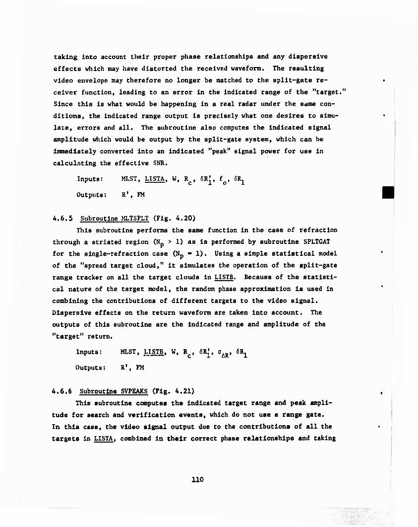
taking Into account their proper phase relationships and any dispersive
effects which may have distorted the received waveform. The resulting
video envelope may therefore no longer be matched to the split-gate re-
ceiver function, leading to an error In the Indicated range of the "target."
Since this Is what would be happening In a real radar under the same con-
ditions, the Indicated range output Is precisely what one desires to simu-
late, errors and all. The subroutine also computes the Indicated signal
amplitude which would be output by the split-gate system, which can be
Immediately converted into an indicated "peak" signal power for use in
calculating the effective SNR.
Inputs: MLST, LI STA. W, R , 6R' fo, 6^
Outputs: R', FM
4.6.5 Subroutine MLTSPLT (Fig. 4.20)
This subroutine performs the same function in the case of refraction
through a striated region (N. > 1) as is performed by subroutine SPLTGAT
for the single-refraction case (Np - 1). Using a simple statistical model
of the "spread target cloud," it simulates the operation of the split-gate
range tracker on all the target clouds in LISTS. Because of the statisti-
cal nature of the target model, the random phase approximation is used in
combining the contributions of different targets to the video signal.
Dispersive effects on the return waveform are taken into account. The
outputs of this subroutine are the indicated range and amplitude of the
"target" return.
Inputs: MLST, LISTS, W, R , 6R', o&R, OR,
Outputs: R', FM
4.6.6 Subroutine SVPEAKS (Fig. 4.21)
This subroutine computes the indicated target range and peak ampli-
tude for search and verification events, which do not use a range gate.
In this case, the video signal output due to the contributions of all the
targets in LISTA, combined in their correct phase relationships and taking
110

I
f mn» J
1 1 • n 1 - 0
\ ■h <*\* 2.32 -'4R
«1 •\ -\ 1 ■ • • «, i c L
LOOP ON «.L TARGETS ,—. 11 ma 11T) 11
1 • 1 ♦ 1 iR,2,l/2 :;:«—»•t'-w«.o<*)«r«-_ <> • 4.0
LOOP 0»! »LL TARGETS (
I •. • [R-R'mn/b 1
f • r ♦ xdT)^2
» END TARGET LOOPry
♦ | F.(F/b)"2 |
Gl ■ f
Gl d ■
• Gl ♦ 6.0 -
dF d
Gl G2 d
. Gl i ■ F
• 4.0
F
G2 d •
• G2 * 6.0 -
dF d
H ■ »,R/3 I • - 1 R.RC.J.4R
1 ■ « ♦'
V HTlL ITU • IT 1
«I yioo
N ■ 40 M • 2 N 4R u/n
■ ' H (G2-GI) T ■ H (G2»GI) FM . 1.028 T/4R,
S • 1.5163 t/T
"' ■ Rc ♦ (--) (1INV<S1
^RETURN J
FM • 10 •60
C RETURN J
Figure 4.20. Subroutine MLTSPLT
I
111
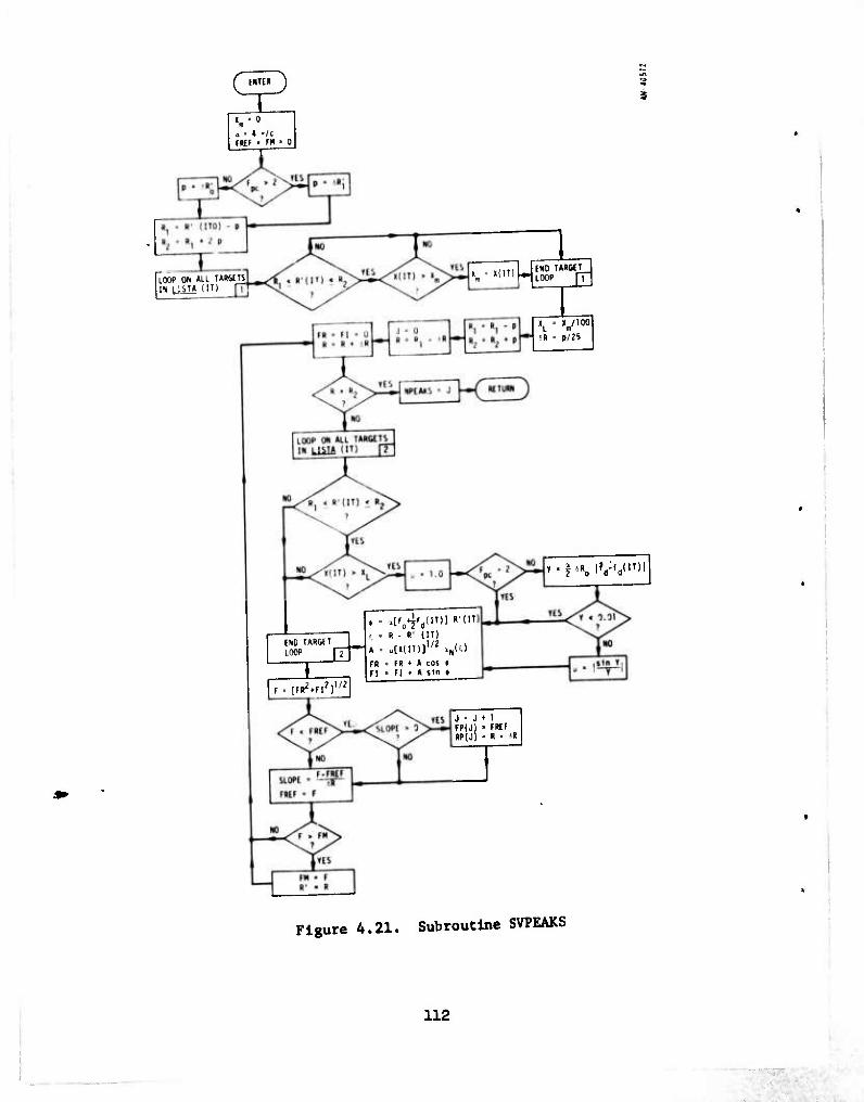
r mm 3 ".•0
a • ♦ «/C • 0
9 S
LOOP OH ALL UR&US IN ysu (It)
"i ' '("'l» [NO TARMT, LOOP m
tl ■ P/2S
END TARGtl LOOP IT
I ,. [^♦ri»]"1
-. . R - K' (IT)
» ■ -[«(H))"2 ,N('.)
FR - FR • A COS • fl . Fl » A sin ♦
y.|fRol?d:<d(lT)|
J ■ J ♦ 1 FP(J) ■ FREF RP(J) = R - >R
Figure 4.21. Subroutine SVPEAKS
112

Into account any dispersive distortions of the received waveform. Is com-
puted and sampled at Intervals within one range resolution distance on
either side of of the primary target of current Interest. The position
and amplitude of the highest peak thus discovered are the outputs.
The subroutine also computes the positions and amplitudes of all
other video signal peaks within the indicated region; these outputs are
not used In the current version of ROSCOE but may be required by more
sophisticated versions to follow.
Inputs: IILST, LI STA. 1T0, 6R', 6R , F , f , f. r 1* o pc o* d
Outputs: R', FII
4.6.7 Subroutine SLNINT (Fig. 4.22)
This subroutine computes the equivalent noise increment, AXj , which
represents the effects of all Individual target Images In the range side-
lobes. Such targets are considered to contribute too little to be worth
Including them in the calculation of the video signal; Instead, they are
each assumed to add to the noise a term proportional to their peak ampli-
tude factor, modified by the signal's current mean sldelobe-to-malnlobe
ratio (taking dispersive effects, if any. Into account). It Is only used,
of course, for signals which have range sldelobes.
Inputs: R', ML:5T, LI STA. LD, SSL, 8., R , W, 6R^, 6R^
Outputs: AX
4.6.8 Subroutine SLNINTM (Fig. 4.23)
This subroutine performs the sal* function in the case of refraction
through a striated region (N- > 1) as is performed by subroutine SLNINT for
the single-refraction case (N ■ 1). Using a simple statistical model of
the "spread target cloud," it computes the equivalent noise Increment,
AXT , which represents the effects of all those clouds or parts of clouds
which lie in the range sldelobes. It Is only used, of course, for signals
which have range sldelobes.
113

AXT • 0
0 = LDSSLS1
5
R1 = AMAX1 {Rc -
R2 = Rc - ? - '5Ri R3 = Rc + ? + 6R1
7 - %, RQ ' fiRö}
R4 = AMIN1 (Rc + J + ^Q. RQ ♦ «RQI
LOOP ON ALL TARGETS IN LISTA (IT)
RI = R; 6R; R2 = R; - 6R'
R, ■ R' + 6R: 3 0 I
R. = R' + 6R^ 4 o 0
&XT = AXT + aX(IT)
END TARGET LOOP
C RETURN J
Figure 4.22. Subroutine SLNINT
Ilk

ENTER
•
AXT » 0
b ■ [U12(^)2]1/2 S/V EVENT
NO
YES
^ = AMAX1 (Rc - f - «RQ' RÖ'' 'S1
^c -? - 6R: - 2.32 t.R R3 ^c
+2 + ^i +2-32^R
R4 - AMIN1 {Rc + ^ + 4R^, R^ ♦ 4R^}
LOOP ON ALL TARGETS IN LISTB (IT)
Rl = Ro ' 6Rö R2 = R; - 6R| - 2.32 oAR
R3=R;+6Ri +2-32aAR
R4 = R; + 6R;
AXT « AXT + aX(IT)
END TARGET LOOP
f RETURN J
Figure 4.23. Subroutine SLNINTM
115
-

Inputs: R^, MLST, LISTS. 1^, S^, S1, oAR, 6R^, ÖRj, W, Rc
Outputs: AX
4.6.9 Function AMBGN(X) (Fig. 4.24)
This function computes the normalized ambiguity function, XJJW *
for a given waveform, as a function of range, X , from the center of the
function. Dispersive effects are included, and it is normalized so that
AM(0) 2 1 . Two different kinds of waveforms are defined: a simple rec-
tangular pulse without frequency modulation (FpC ■ 1), and a pulse-
compression signal (FpC >> 1} whose characteristics fall roughly between
those of Hamming- and Hannlng-weighted waveforms. It should also be noted
that the ambiguity function is computed only as a function of range: In
affect, it Is assumed that $ (the doppler frequency difference) ■ 0;
wherever doppler mismatch effects are required they are calculated separately.
7 ,e reason for this Is that function AMBGN attempts to take into account
the waveform distortions caused by dispersion along the propagation path(s).
Although this can be done for the range coordinate, an exact formulation
for the dispersive effects on the doppler coordinate has yet to be derived |
an approximation, which separates the two dimensions of xN » J-8 currently
used.
Inputs; X, F , «R;, 6Rj, A^ LD, S^
Outputs: xN
4.6.10 Function QINVU) (Fig. 4.25)
This function is used by the split-gate range tracking subroutines,
SPLTGAT and MLTSPLT, to locate the apparent target point with respect to
the center of the range gate. This function is specifically matched to the
weighted waveform (FpC >> 1) mentioned above, and would give the correct
range of the target point if there were only a single target in the resolu-
tion cell and if there were no dispersive distortion of the signal. In the
presence of either or both of these "anomalies," an Incorrect position is
computed for the target, which is Just what a real split-gate range tracker
would do under the same circumstances. See Appendix C for details.
116

0/S6f-NV
r\
v_y
c o
CM
2
U7

f ENTER J
X = ABS(S) Y = SIGN (l.O.S)
X Z 0 0
0.0999 0.1000 0.1993 0.2000 0.2975 0.3000 0.3940 0.4000 0.4884 0.5000 0.5801 0.6000 0.6686 0.7000 0.7536 0.8000 0.8347 0.9000 0.9115 1.0000 0.9837 1,1000 1.0512 1.2000 1.1138 1.3000 1.1714 1.4000 1.2239 1.5000
X Z
1.2714 1.6000 1.3138 1.7000 1.3514 1.8000 1.3843 1.9000 1.4127 2.0000 1.4368 2.1000 1.4569 2.2000 1.4733 2.3000 1.4865 2.4000 1.4966 2.5000 1.5042 2.6000 1.5095 2.7000 1.5130 2.8000 1.5151 2.9000 1.5160 3.0000 1.5162 3.1000 1.5163 3.1416
QINV - Y*Z
r RETURN J
QINV « YTT -m/ RETURN J
FIND Z(X) BY INTERPOLATION OR OTHERWISE IN THE FOLLOWING TABLE:
Figure 4.25. Function QINV
US

1
Inputs: s
Outputs: QINV
4.7 THRESHOLDING AND RADAR MEASUREMENT ERRORS
As explained earlier, the output of subroutine RADMODS is the "apparent"
target coordinates (R'.u'.v'), which include the effects of the environment
on the radar's measurements but do not include the inherent errors of the
radar itself. These are added by another subroutine, MEASERR, called not by
RADMODS but by the event subroutine that called RADMODS.
A final subroutine, XTHRSHS (also called by the event subroutine),
compares the RADMODS output Z0 with a threshold signal-to-noise-plus-
clutter ratio.
4.7.1 Subroutine MEASERR (Fig. 4.26)
This subroutine Just adds radar measurement and bias errors tj the
apparent target coordinates which are output by subroutine RADMODS. The
calculation involves selecting random samples from appropriate zero-mean
distributions having variances given by a standard radar formula, and adding
fixed biases as required.
Since the angular coordinates are not measured in search and verifica-
tion events, but are merely set equal to the commanded receive beam axis
coordinates (u0,v0), subroutine MEASERR does not compute any measurement
errors for these coordinates for these events. Then we have Just
u = u1 and v = v' m m
The bias errors, 6R. , äu. , 5v. , remain constant for each radar
throughout a given computer run. They may be input directly by the user.
An alternative procedure is to input the standard deviations of their dis-
tributions for each radar type; then at the beginning of each run the values
of (5R. , äu. , 6v. to be used for each radar during that run may be drawn
119

iui|Nimmium.4iHi-. "■ÜIWll'MP'PL'P.w "^ ^ ■ ■
ENTER 3 L2 B2"1
A2 t LD BR R z0J
1/2
SELECT RANDOM NO.
6RrC G(0, aR)
SELECT RANDOM NOs. 6urcG(0, ou)
6vrc6(0, ov)
RJJJ = R' + «Rjj + 6Rr
—m*C RETURN J
>
«n,3 R' + 6Rb + 5Rr
! um
= u' + 6Ub + 6ur vm = v' + 6Vb
+ 6U 1
C RETURN j
Figure 4.26. Subroutine MEASERR
120

as random samples from the appropriate zero-mean Gaussian distributions.
In either case, the values of these bias errors for each radar are stored
In appropriate datasets for use In subroutine MEASERR.
The random measurement errors, 6R , 6u , 6v , are sampled each r r r
time from zero-mean Gaussian distributions with standard deviations a R*
'lances o
these distributions are found from a formula of standard type:
a , a which are computed within subroutine MEASERR. The variances of
q q Zo
«V,fl^Q "„•" where "q" stands for R, u, or v , respectively. Here Z0 Is the out-
put signal-to-noise-plus-clutter ratio from RADMODS. The six constants
{A ,B } are input by the user for each radar type; their values are
usually known as a result of routine error analyses of a given radar type.
The factor pq In the above equation Is related to the spread in
effective range resolution due to dispersion. It obviously does not apply
to angular measurements; hence, p m p = 1 . For range measurements, it
may be shown that p = L , where L Is the dispersive loss factor cal-
culated in subroutine REF1S for the current radar waveform under present
conditions.
The outputs of this subroutine are (R ,u ,v ). Note that in Sec. 3, m m m
these outputs were denoted In different ways for different event types:
• Search: R
• Verification: (R^Uy.v^
• Track Initiation: (R.^.v.) and (R-.u-.v.) as appropriate
• Track: (R ,u ,v ) m m m
121

Inputs: Zo, LD, (R'.u'.v1), {AR,Au,Av,BR,Bu,Bv}, {öR^öu^.öv^
Outputs: (R »u .v„) m m m
A.7.2 Subroutine XTHRSHS (Fig. 4.27)
This subroutine determines, In a very simplified manner, whether the
output slgnal-to-nolse-plus-clutter ratio (Z0) computed by subroutine
RADMODS does or does not cross a predefined detection threshold. The de-
termination Is made simply by computing the output value equivalent to the
Input threshold (S/N) which Is one of the parameters associated with the
basic waveform/event dataset, and then comparing Z0 with this value. The
output, XTH , is a Hollerith-valued constant, either NO or YES.
Inputs: IFDET, Zo, (S/N)Ti
Outputs: XTH
122

XTH ' 2HN0 1
RETURN 3 <
COMPUTE OUTPUT THRESHOLD:
XTH - 3HYES
C RETURN J
Figure 4.27. Subroutine XTHRSHS
123
«■k

PROPAGATION
The following propagation models have been Included in ROSCOE:
1. Absorption
2. Fireball Noise
3. Refraction
4. Clutter
5. Low-Altitude Fireball Multipath
•
5.1 ABSORPTION
Absorptions due to fireballs, betas, delayed gammas and neutrons,
and prompt X-rays and neutrons are computed when subroutine ABSORB is
called in the program. This routine in turn calls a series of subroutines
which perform the individual absorption calculations. The calculations
are terminated if at any time the Integrated absorption (DBSUM) exceeds
a specified threshold (DBMAX).
5.1.1 Assumptions
The attenuation calculation consists of a numerical integration of
the non-deviative incremental absorption equation
-. 7.3 x 10"8N (v + v .) 9A e em ei
8r f2 + (0.775v + v ,)2
em ei
dB/cm
where N * electron density, cm -3
f * radar frequency, MHz
average electron-neut
frequencies divided by 2-n « 10" .
v ,v . > average electron-neutral and electron-ion collision em ei ,
The non-deviative assumption, although not strictly valid, is made to
reduce computation time. It permits one to decouple the absorption and
12U
-

WWnwww
refraction calculations so that a relatively fast absorption computation
can be made along the path of interest.
The error Introduced by this assumption Is expected to be small
except under severe refractive conditions; under these conditions, the
system Is probably seriously degraded by refractive errors to the extent
that a precision absorption calculation Is unwarranted.
5.1.2 Procedure
Subroutine ABSURB computes absorption between two points due to all
significant radiation sources. This subroutine calls FBABS to compute
fireball and dust absorption, and DELABS to compute absorption due to all
other sources.
Fireball absorption is computed by simply integrating the Incremental
absorption as the radar line-of-sight Intersects each fireball region. A
more complex integration procedure is used in DELABS. The scheme follows
these steps:
1. An array of mandatory points on the path of interest is found
where absorption may be significant (e.g., for fireball ab-
sorption the point of closest approach to the fireball center
is used).
2. The mandatory points are ordered in range from the radar—
shortest range first.
3. The integration is started at the first mandatory point and
proceeds down in range until one of the following occurs:
(a) range - 0; (b) incremental absorption falls below some
minimum threshold; (c) incremental absorption Is less than
5% of the total Integrated absorption.
4. The integration is then continued u£ in range from the first
mandatory point until either the maximum range Is reached
(e.g., the range to the target) or 3(b) or 3(c) is satisfied.
125

5. For subsequent mandatory points that have not been Included
in the above integration, the same procedure is followed,
except that when integrating down the path the minimum or
limiting range is the last integrated point rather than 0.
In the integration procedure, a variable integration step size is
used depending on the magnitude of the current and last computed values
of Incremental absorption. The increment in slant range DELING is given
by:
DELING - AMINKAMAXl(DELING' * DBING1/DBING,DSMIN) ,DSMAX)
where DSMIN - .5 * DSNOM
DSMAX - 2 * DSNOM
DSNOM - AMINKAMAXl (DSNOM1, .1 x IQ5), 5 x 10⁵)
DSNOM' ■ An internally set value (e.g., .05 * target altitude
for fireball absorption)
DBING1 - Incremental absorption for last calculation (taken
as zero initially)
DBINC m Gurrent calculated incremental absorption
DELING' - DSNOM for first integration step
5.1.3 Flow Gharts
Flow charts for the absorption subroutines are presented in Figs. 5.1
to 5.3.
There are a number of flags and variables used in the code to in-
dicate integration direction and integration limits. Some of these are:
SI m slant range to the ^th mandatory point
126
fxmtutm»mm*m . I

( INPUT DBMAX SET DBSUM = 0 ̂ >
GET PROPAGATION INPUTS DATASET TO GET ELEVATION, uv. SMAX, MP
Figure 5.1. Subroutine ABSORB
S2 = maximum slant range already integrated (=0, initially)
k - integration direction (denoted DIRECTN in code) - +1, up
path; -1, down path
L m flag to indicate current integration step is starting at
point of closest approach (denoted ATP01NT in code) « 1,
if a mandatory point; 0, otherwise
kl - flag to indicate integration has reached lower integration
limit (S2) (denoted ATSMIN in code) - 0, if at S2; 1,
otherwise
5.1.4 Inputs and Outputs
Subroutine ABSORB is called by subroutine RAD1S of the radar
signal processing module. RAD1S feeds ABSORB the radar position,
current calculation time, radar frequency, and maximum one-way absorption
127

[ ÜMPUTI RANGI 10 FB (SA), tXTFNI Ot fB ALONG LOS :PL1
x: COMPUTl STEP SIZE (CSNOM) mo NUMBER nr STEPS (NSTCPS)
TNO
COMPUTE INCREMENTAL ABSORPTION (DBPKM)
CALL ABS1NC
7 COMPUTE TOTAL ABSORPTION
DBSUM DBSUM ♦ DBPKM x DSNOM
COMPUTE TOTAl ABSORPTION
DBSUM - DBSUM + DUST ABS.
NO ' DBSUM OBMAX
f RETURN )
Figure 5.2. Subroutine FBABS
128

ijwaiiiii.iii»iiwiiliii
Wit \_ U' WHIMII*' ; r ^ POilll »'«SC
r "l I !«< . ■ • ,
.- I- , ■aiiitLiii
fin JP IH'I'.«'!.' v w j im1 sun «iw, ',>-"H JSW«. fiWX, w
; ««.I • H' PI in
t
«1 •'.
I-
r i
!
^ I
CO«!«' !t" ■ I« [ail* I t I H 10 IMI- I»' >l I—(DtllUt J:«««
I I.OÜOOIM'1. 1- 1 [Q.ll Si Uj
! MSOtPIlO«
i [oil«')
.«L1J..C,S?>»^>. Kill« 0€i.l>K . r „ — i
>i . q -■ I«' f _ 1
Uli Mi 1 U*iüP ■ »b^ ■
WIN.
J «i tu«« |»~ 1M„
<r »« «i ■ u
r—
Y- <5 • I • >1—_J(»l«.l ■ otl».
T_x_ . J _ _DeilKI_. Ml« _ ,
im.i »si ^iiinGUiu»
OIWCTIIM I» • -ti
Figure 5.3. Subroutine DELABS
129

of Interest (equal to the total dB required to reduce the slgnal-to-noise
ratio to a value Just below the detection threshold). ABSORB returns the
total one-way Integrated absorption over the curtent path of Interest.
The Inputs and outputs of the absorption routines are summarized as
follows:
ABSORB Inputs: DBMAX Maximum one-way absorption of
interest, dB
TIME Current time, seconds
FREQ Radar frequency, MHz
R(3) Radar position, cm
ABSORB Output! DBSUM Total integrated absorption, dB
FBABS and DELABS Inputs: DBMAX
R(3)
UV(3)
SMAX
ELEV
MP
TIME
FREQ
Maximum absorption of interest, dB
Radar position, cm
Unit vector along radar line-of-
sight
Maximum range of interest, cm
Current radar beam elevation, deg
Pointer to mandatory-points dataset
Time, seconds
Radar frequency, MHz
FBABS and DELABS Output: DBSUM Total integrated absorption, dB
5.2 FIREBALL NOISE
All fireballs in the main beam of the radar antenna are assumed to
be potential noise sources in ROSCOE. Subroutine NOISE computes the
effective noise temperature along the radar line-of-sight from each
fireball satisfying this condition.
130

The noise temperature calculation performed In ROSCOE attempts to
account for non-uniform temperature and emlsslvlty distributions through
the fireball edge by numerically integrating through this region. The
form of the expression for the noise temperature contribution from a
particular fireball is
-0'UM Tef - 10 * T ff x GAINO,*)
where
"0-1ABBS Teff " |T X e '" 10 " dii ■ß
GAIN(9,4>) 'JJii ain * d* de
and A^R ■ cumulative absorption from outer edge of fireball to
radar (or next fireball If there Is more than one), dB
T ■ temperature at point of Interest along path I , 0K
e ■ emlsslvlty at point of Interest
)BINC -0-1AD! - 1 - 10
A_R_ ■ cumulative absorption from outer tfdge of fireball to
point of Interest inside fireball, dB
V _ „_ ■ incremental absorption for point of interest, dB
5.2.1 Assumptions
The following assumptions are made in the NOISE model:
1. The radar beamwldth is narrow and the main contributors to
the noise temperature are fireballs in the main beam.
131

2. Integration over the main beam pattern is used to find the
effective contribution to the noise for each fireball, but
the noise is propagated along a path coincident with the
antenna pointing direction. This simplifies the noise
absorption calculation since only a single path has to be
considered for all fireballs.
3. A numerical integration is performed through the fireball
edge to account for non-uniform temperature and emissivlty
distributions as discussed above.
5.2.2 Procedure
The noise calculation follows these steps (see Fig. 5.4):
1. An array of mandatory points Is found where noise temperature
may be significant.
.
RADAR
Figure 5.4. Fireball Noise Integration Procedure
132

2. The points are range ordered—shortest range fiom the radar
first.
3. The calculation is started at the first point and proceedf
down In range until the temperature-emissivity product drops
below i07a of the svstem temperature. At each step along the
path, the temperature-emissivity product and Incremental
absorption are stored—step (c).
4. After reaching this point, the calculation reverses direction
and begins Integrating out In range over the fireball until
the starting point is readied (halfway over the fireball
Intersection path)—step (d).
5. The absorption is tiien computed from the fireball edge (SPT)
to the radar ''or to the next fireball down In range (S2)) —
step (e).
6. The procedure then returns to Mandatory Point No. 1, and
continues integrating out over the fireball until the upper
edge is reached (i.e., temperature-emissivity again falls
below 10r' of the system temperature). This [>ulnt is S2
for the next sequence of calculations—step [t),
7. The procedure Is repeated, beginning at the next mandatory
point. This is continued until either all mandatory points
are covered or the cumulative absorption along the path is
larger than 30 dB.
5.2.3 Flow Chart
A flow chart of subroutine NOISE is given in Fig. 5.5. A definition
of some of the flags and variables used in the routine follows:
SI ■ slant range to the point of closest approach to the _ith
fireball (see Fig. 5.A).
133

INITIALIZE INTEGRATED PARAMETERS
S - 0.. S2 ' 0.. I • 1
SET UP INTEGRATION STEP SUES (DSNOM. DSMIN, DSMAX) AND RANGE TO It* POINT (SI)
CONVERT Ith POINT TO EARTH CENTERED COORDINATES
COMPUTE INCREMENTAL ABSORPTION (DB1NC)
OBINC • DBPKM * DELINC
J . J + !
S - SI, J ■ C L • 1. DELINC - OS'iuM K • -1, 0B1NC1 • J IF (LEQ.') S2 • 0
(TO NEXT PAGE)
I.lgure 5.5. Subroutine NOISE
13k

PWU 11 WW.IM^WJ; " I»'!- P** "jl '.'ff IJPf ..W^ ■
I
CALCULATE TENP-EmSSIVITV (TENS (J)) ADO ACCUMULATED ABSORPTION (DBSUM)
STARTING WITH LAST POINT (J) START IHTEGRATING UP PATH ACROSS FIREBALL
IF (N.GT.O) M - 0
SET UP PARAMETER FOR ABSORPTION CALCULATION
FIND POINT 1 AND POINT 2 AT EDGE OF FIREBALLS
CALL DELABS COMPUTE TEF AND ABBS
1
Figure 5.5 (Cont.)
135

S2. ■ range to the upper edge of the (1-1 )th fireball already
Integrated over (see Fig. 5.4).
K - flag indicating the integration direction (denoted DIRECTN
in code) - +1, if integrating up the path; -1, if integrat-
ing down.
Kl - flag indicating that the lower integration limit (S2) has
been reached (denoted ATSMIN in code) - 0, if at S2; 1,
otherwise.
L > flag indicating that the integration step is currently at
a mandatory point (denoted ATPOINT in code) - 1, if at
mandatory point; 0, otherwise.
J m number of integration steps when integrating over fireball.
M ■ counter to loop over J integration steps.
5.2.4 Inputs and Outputs
The NOISE routine is called by subroutine RAD1S of the radar signal
processing module. The inputs and outputs of the NOISE routine are
defined as follows:
Inputs:
Output:
TSYS
TIME
R(3)
FREQ
TEF
System temperature, 0K
Current time
Radar position, cm
Radar frequency, MHz
Effective noise temperature, 0K
136

"" ' - >»' ....H—»-- - —,,- »<Jll , ■.■.»«■IIIIJUI .-^ uiW. gpi... qnvimrj
'
5.3 REFRACTION
Roscoe makes the basic assumption that the number of possible
propagation paths to the target In the malnbeam Is either one (correspond-
ing to the smoothly varying electron density gradient region), or much
greater than one (when strlatlons are present). These two cases are
discussed separately.
5.3.1 Gross Refraction
In this case, a ray trace is performed, starting at an altitude of
60 km along the radar beam-pointing direction and ending at a point that
may be displaced from the target but is at the same range from the radar.
The incremental range and angular bias errors at each step are given by:
3R as
1.59 x 10³N
7 ^T I Zir x 10° J 1 2. loT f2 + (vem+vei)2
36. -1.59 x lO'TN , 1 _ el
3S
(2lTXl06)2[f2+^m+Vei)2'
137

ii" ■. WAWWH. c . i..p^.,^.,,..^^-^ , ,„,. .,w.|l t., w.„,^J,„rr,.,^^ tmmil
--»wrars
where
U ■ real part of the Index of refraction
- 1 - 3.18 x IO'N
\2v x io6) ff |2n 106)'|f2+ (vem + vel)2
1/2
N » electron density, cm -3
VN - electron density gradient In the 1th direction.
-3. cm /cm
f - radar frequency, MHz
average electron-neut
frequencies divided by 2v x 10^
v ,v ■ average electron-neutral and electron-Ion collision em el
It Is assumed that the total angular error obtained from this procedure
Is not large, so that If the beam Is rotated just this amount, the *
refracted beam will hit the target.
5.3.2 Refraction due to Strlatlons
For refractive effects due to Ionized strlatlons (the latter case
mentioned above), the assumption Is made that the electron density does
not lead to excessive departures of a ray In the beam from Its nominal
smooth trajectory. With this assumption, It Is possible to develop a
theory which describes. In statistical terms, the effects of the
electron density fluctuations.
A refinement of this procedure would be to Iterate on the beam pointing direction until the refracted beam does hit the target.
138

iyHPmB»»IJ I Lppj,!»».!!^!!»! I I.Mtt^a*'!11- I, .1II,<J"1»-".»J'»"JH, njunp^ii^jini m iii.iiyMillllJIIIII.im I ,ll !■ LI ii» ■ - ■■ ■- '"
The theory presented here, termed the "thin screen approximation,"
differs from previous models ' In that It systematically develops the
"dogleg" range error and phase terms. Because of these differences, a
rather complete description of the model Is given In Appendix F.
5.3.3 Procedure
Both computations described above are calculated within subroutine
REFRCT In ROSCOE. The procedure follows these steps (see Fig. 5.6):
1. The radar beam Is assumed to be straight to an altitude of
60 km.
2. At this point, an Incremental range step size (DSINC) Is
selected and the deflection of the ray over this range
segment is computed.
3. In addition, random erro.'s due to strlatlons over this
range segment are computed and projected to the target
range (SMAX).
4. The procedure continues in this way until the range from
the radar to the point on the refracted ray (PT.) is equal
to the target range.
5. When this condition is satisfied, the program outputs bias
and random errors in range, azimuth* and elevation at the
final point, the integrated electron density over the path,
and the angle between the line-of-slght and the magnetic
field at the point of maximum electron density along the
path.
5.3.4 Flow Chart
A flow chart of subroutine REFRCT is presented in Fig. 5.7. This
routine requires information from several phenomenology routines and
calls other propagation models as shown. A description of some of these
subroutines follows.
139

■
TARGET
PT (J)
H = 60 km
Ml U-l
FUZZ BALL DUE TO STRIATIONS (RNGFUZ. AZFUZ, ELFUZ)
SMAX = SLANT RANGE TO TARGET
RNGBIAS = TOTAL RANGE BIAS ERROR DUE TO SMOOTHLY VARYING REFRACTION
PT(J) = COORDINATE OF END POINT OF REFRACTED RAY PATH AT RANGE OF TARGET
RNGFUZ, ELFUZ, AZFUZ ' RMS UNCERTAINTY IN END POINT
DSINC1 = INCREMENTAL RANGE STEP
' AMAX1 (0.5 * DSNOM, AMIN1 (2. * DSNOM, 0.05/DEFL * DSNOM))
DSNOM " AMIN1 (50., RANGE CORRESPONDING TO 10 km ALTITUDE STEP)
DEFL - AMAX1 (INCREMENTAL DEFLECTION IN AZIMUTH DIRECTION, INCREMENTAL
DEFLECTION IN ELEVATION DIRECTION)
Figure 5.6. Ray Trace Procedure
lUO

G
CUIVEKT CURRENT POINT TO tAIITH CENTERED COdlDIMTE
crwuif PDOWT ENCKlf DEPOSITION (ED) «T POINT
ULL FIELD (PT. F) C«U UNITV (F, FUVUND)
COHPUTE FUZZ BALL «HOUND BIASED POINT •T TADCET RANGE (AZfUZ, ELfUZ, RNGFUZ)
f RETUKN J
FIND RANGE TO «IT ^OINTiS) AND RANGE FROM THIS POINT TO TA«G£T (SPT)
FIND UNIT VICTOR (V?) PERPENDICULAR TO CURRENT LINE-OF- SIGHI
GET ELECTRON DENSITY GRADIENTS IN ELEVATION AND «2IHUTH
USE GRADIENTS TO COMPUTE SNOCTH BIAS REFRACTION
COMPUTE INCREMtNT'.L STEP SIZE (DINC) FOR STRIATION CALCULATION
CONFUTE RNS POSITION UNCERTAINTIES DUE TU REFRACTION
CALL TTRCTUT —
rALL FUZINC
CONPUTE RANUOM ERRORS IN RANGE, ELEVATION AND AZIMUTH
FIND NUT INTEGRATION POINT IN RAV TRACE USING BIAS ERRORS
Figure 5.7. Subroutine REFRCT
1J+1
Phenomenology Subroutines
ELDENS Provides electron density and temperature at a
point due to all sources
GRADNE Computes electron density gradient at point P
in a specified direction V
STRCTUR Computes structure of a striated region
BFIELD Returns direction of B-field at a point
Other Propagation-Related Routines
COLLF Calculates electron-neutral and electron-ion
collision frequencies
BIAS Computes smooth bias refractive errors
FUZING Computes RMS position uncertainties due to
refraction in striated medium over the path
length
5.3.5 Inputs and Outputs
Subroutine REFRCT is called by subroutine REF1S of the radar
signal processing module. The inputs and outputs of REFRCT are:
Inputs: TIME Engagement time, s
SMAX Slant range to target, cm
R(3) Radar position, cm
FREQ Radar frequency, MHz
Outputs: NP Number of possible paths to target
XNE Integrated electron density
REFRAC(l-3) Bias errors in R,A,E coordinates
REFBAC(4-6) Random errors in R,A,E coordinates
REFRAC(7) Angle between LOS and B-field at
point of maximum electron density
142

SIGBAR Amplitude gain factor for each
return
XMU Angle between major axis of uncertainty
ellipse and the u-axis in sine space
The refraction errors are used to compute the apparent target position
that the radar "sees." The integrated electron density is used in the esti-
mation of the pulse dispersion, and the angle between the LOS and B-field
at the point of maximum electron density is used to determine the Faraday
rotation angle, if appropriate.
5.4 CLUTTER
Radar backscatter or clutter can occur from a variety of regions
following a nuclear burst; in general, whenever the beam traverses a
region in which the dielectric constant varies. Clutter sources such as
dust, fireballs, and field-aligned regions are treated in ROSCOE.
■ • 5.4.1 Assumptions
The following assumptions have been made for the clutter model:
** 1. The absorption of the clutter return from the region surface
is computed along the path between the region's center and
the radar. This allows a single path absorption integration
to be used for each clutter source.
2. The solid angle subtended by the clutter source is divided
into 25 projected area segments for incremental clutter
calculations. This makes the clutter integration independent
of the geometry of the region.
* Faraday rotation is considered when a linearly polarized radar antenna is specified in the input.
** This absorption calculation includes the absorption through the gammas surrounding the fireball, if appropriate.
Ik3

3. The total clutter return Integrated over the beam pattern
is multiplied by a factor which represents the fraction of
the clutter source in the compressed and uncompressed
range cells; that is, a detailed integration is not per-
formed over the range cell.
5.4.2 Procedure
The total clutter power reaching the radar from all clutter sources
is computed in subroutine FBCLTR. This routine determines if a clutter
source is in the compressed or uncompressed range cell and, if it is,
computes the fraction of the cell covered. The clutter power is then
integrated over the antenna beam pattern in subroutine CLINT and
returned to FBCLTR. Finally, the one-way absorption is computed from
the source to the radar and the clutter power is degraded by this factor
times the fraction of the range cell subtended by the source.
The clutter integration in CLINT follows thede steps:
1. Define the integration step size (incremental area) to be
small compared to the extent of the source. (A maximum of
25 steps is allowed.)
2. Direct a vector from the radar to the center of each of
these area segments.
3. Compute the clutter power per unit area along the defined
vector intersecting the source. Degrade the clutter power
by the antenna angular gain.
A. Sweep in azimuth and elevation. Integrating over the portions
of the source which contribute significantly to the total
clutter.
An individual calculation is skipped when (1) the vector does not
intersect the geometric region defining the source, or (2) the individual
segment contribution is a small fraction of the cumulative clutter power
Ikk

(this Is necessary for fireballs with diffuse edges). The Integration
Is terminated when all 25 steps have been considered.
The Incremental clutter Is computed In subroutine CLUTINC, which
Is called by CLINT. It In turn calls routines to get the surface
reflection coefficient and applies a doppler loss to the Incremental
clutter power which Is computed by comparing the doppler shift of the
clutter source with the doppler shift of the target. The doppler loss
Is computed from the following equation:
FDOP - ABS[(sln X)/X]3*4
where
X - j-ABS(FDT - FDC) n
B - noise bandwidth. Hz n *
FD_ - expected doppler shift for the target based on past
tracking measurements, Hz
FD. - doppler shift of the clutter source
2f R --2-£, Hz
c '
f - radar frequency, Hz
c - speed of light, cm/s
R ■ velocity of the clutter source toward the radar, cm/s
Thus, the equation for the Incremental clutter power per unit area
(AC/AA) Is
77 - S x FDOP x ALBEDO AA
1U5

where S ■ signal for this computation
ALBEDO ■ surface reflection coefficient
The total clutter power for this source is then given by:
AX x 10
DBSUM 10 /r GAIN dA
where GAIN ■ antenna gain in the direction corresponding to the
_lth area segment
AX - fraction of range cell subtended by the source
DBSUM - total abiorption from the source to the radar
5.4.3 Flow Charts
Figures 5.8 and 5.9 are flow charts for subroutines FBCLTR and
CLINT. Some of the other subroutines and functions called by these
routines are listed below.
ABSORB
CLUTINC
EXTENT
GOA
SLDANGL
Computes the absorption from the fireball
surface to the radar (see Sec. 5.1)
Computes the Incremental clutter power per
unit area for the ith source
Computes the range to the surface of the
clutter source and the extent of the source
Computes the angular gain for an input vec-
tor direction off-beam center (see Sec. 4.4.2)
Computes the solid angle subtended by the
clutter source
11+6

I ( REQUEST N V OATASETS )
_ZIZ_ INITIALIZE SCTRC -0.0
I DEFINE RANGE CELLS
c RETURN
LOOP OVER ALL POTENTIAL_SOURCES, _ DEPfNE RANGE TO SOUficT AND THICKNESS
X3 • FRACTIONAL EFFECT OF SOURCE ON OUTPUT (X3 < 1)
X3 - 1 - FRACTIONAL EFFECT OF SOURCE ON OUTPUT
CALCULATE CLUTTER POWER AT REGION SURFACE
CALL CLUTRrB
DEGRADE C BY ABSORPTION TO fb SURFACE.
JJULTIPLYJYJtf CALL ABSORB
VES
3
RETURN ")
Figure 5.8. Subroutine FBCLTR
147
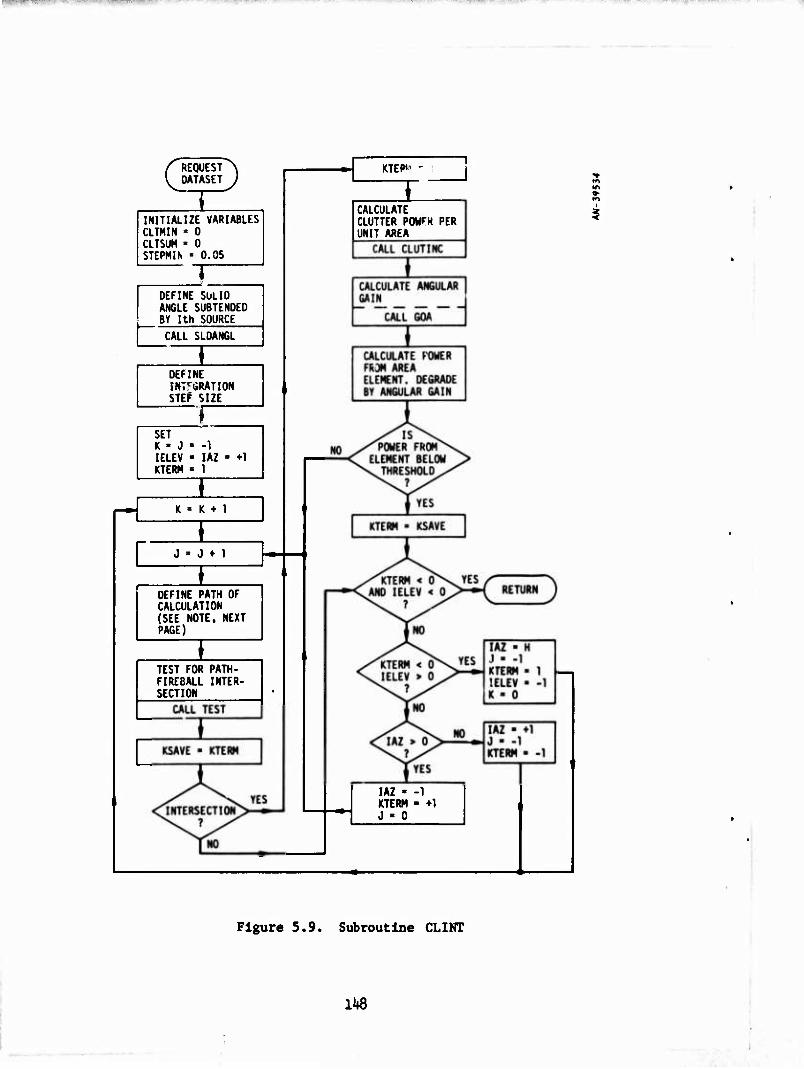
j, P»I .«II u.11 HI J i .K ' ■Mini i,Pin., mm&G*i'QV*w — . .
/"REQUEST^ l DATASET J
INITIALIZE VARIABLES CLTMIN • 0 CLTSUM • 0 STEPMIN • 0.05
1 DEFINE SOLID ANGLE SUBTENDED BY Ith SOURCE CALL SLDANGL
DEFINE JNTfGRATION STEP SIZE
1
K ■ K ♦ 1
L j • j ♦ i
ZU DEFINE PATH OF CALCULATION (SEE NOTE, NEXT PAGE)
TEST FOR PATH- FIREBALL INTER- SECTION
SET K ■ J • -1 IELEV - IAZ • *} I KTERM ■ 1
KTE IK-
CALCULATE CLUTTER POMFR PER UNIT AREA
in
to
i
IAZ - -1 KTERM - ♦! J • 0
Figure 5.9. Subroutine CLINT
lk8

■■■ ....»I».»1 "- ■--^■..t.w.^.. HKiii.. i^BH.ii .■...».^ ..»■■-■WIW .' i.'WU'-V.'^WjUWWi, '■■-
5.4.4 Inputs and Oatputs
The Inputs and outputs to the three main routines which make up
the clutter module (FBCLTR, CLINT, CLUTINC) are listed in Table 5.1.
5.5 LOW-ALTITUDE MULTIPATH
The low-altitude multipath model consists of four subroutines.
The main routine (MLTPATH) is called by subroutine REFLST1 (see Sec. 4.4.1).
It determines if there are any additional target images caused by low-
altitude fireball multipath which might interfere with the primary target
signal. The other routines perform the following supporting computations:
BOUNCE—Computes the apparent target image position and signal
amplitude for the three additional returns that can occur for
each signal
AMPREF—Computes the amplitude reflection coefficient at the
designated specular reflection point on the fireball surface
SPCULAR—Computes the specular reflection point on the fireball
surface
5.5.1 Assumptions
The following assumptions have been made in the MLTPATH model:
1. Only fireballs below 60 km altitude are considered as
possible reflecting surfaces.
2. Multiple reflections are ignored; that Is, only a single
reflection between any object/fireball pair is considered
(but all pairs are considered).
3. Differences in attenuation along the reflected path as
compared to the direct path are ignored in computing the
received signal.
In addition, some simplifying assumptions are made in AMPREF
and SPCULAR:
lk9
aiiiMn MOa

P...1- II^II !--■ ipi, .,„ m .ix.,....!...- - ».■Wi.|i»J>W.J., .-
TABLE 5.1
INPUT/OUTPUT DATA FOR CLUTTER ROUTINES
FBCLTR Inputs (from calling sequence):
FBCLTR Inputs (from datasets):
FBCLTR Output:
CLINT Inputs:
CLINT Output:
CLUTINC Inputs!
CLUTINC Output!
RTARG Range to target, cm
XT Total noise power, erg/s
T Time of calculation, s
FREQ Radar frequency, MHz
R Earth-centered coordinates of radar, cm
BVEC Boresight vector of radar
DELRU Uncompressed pulse range resolution, cm
DELRC Compressed pulse range resolution, cm
FDBAR Expected doppler shift, MHz
SLRED Range sidelobe reduction factor
SNMIN Signal-to-noise threshold
FBLIS List of clutter sources
SCTRC Total clutter power reaching receiver,
erg/s
DSPFB Pointer to clutter source of interest
FPC Pulse compression ratio
BN Noise bandwidth
R Radar coordinates, cm
BVEC Boresight vector
CLTR Clutter power output (at surface of
region), erg/s
DSPFB Pointer to clutter source of interest
V Vector from radar to source point of
present calculation
R Earth-centered coordinates of radar, cm
FPC Pulse compression ratio
BN Noise bandwidth
FREQ Radar frequency, MHz
CLTINC Incremental clutter from ith source,
erg/s
150

, i 1,1 .UPBHU.I.iillJ,
1. The amplitude reflection coefficient Is computed, using the
REFC0 routine, by Inputting the proper angle of Incidence
of the radar beam.
2, The fireball Is spherical and the reflection point lies on
the surface at the point of closest approach to the direct
llne-of-slght (see Fig. 5.10).
5.5.2 Discussion
Flow charts are presented for subroutines MLTPATH and BOUNCE In
Figs. 5.11 and 5.12. The MLTPATH routine accesses the radar signal
processing dataset to get the list of primary targets that have been
acquired. It also accesses the propagation Inputs dataset to get the
mandatory points list, which are the points of closest approach of the
fireballs to the current llne-of-slght. The routine then loops on each
object/point pair for those mandatory points where the associated fire-
ball is below 60 km and calls subroutine BOUNCE.
I S 5
TARGET
Figure 5.10. Specular Reflection Point
151
i,-i,»»,winT»nmro -i■ ^■"■I'wy.wwiw"'
ACCESS RADAR SIGNAL PROCESSING DATASET (NRSP)
LOOP ON ALL TARGETS IN "LISTA" (LIST RS (NRSP)) IN REVERSE ORDER
ACCESS PROPAGATION INPUTS OATASET (NPI)
LOOP ON ALL MANDATORY POINTS (MPLIS MP (NPI))
COMPUTE FIREBALL ALTITUDE FOR THIS MANDATORY POINT. ALTFB = XMAX (FBPOS) - RBODY
CALL BOUNCE (GET RUV COORDINATE OF APPARENT IMAGES AND AMPLITUDE OF RETURN "A")
CREATE A TARGET IMAGE DATASET FOR i • 1. 3 PATHS
CALL GOA (GET SIGNAL DIGRAD DUE TO TARGET OFF-AXIS-"F2")
COMPUTE TOTAL SIGNAL DEGRAD
xi = o * FX
UNLOCK RS. DATASETS
COMPUTE OFF-AXIS FACTOR Fc FOR EACH PATH:
F2 = F1*F2*A
F3 = (F2*A)"2
WHERE: Fl » DIRECT PATH FACTOR
' PI -*{ RETURN J
PUT THIS (1th) TARGET IMAGE ON "LISTA" IN INCREASING ORDER OF RANGE
Figure 5.11. Subroutine MLTPATH
152

• "WIM P. Hl
CALL SPCULAR (COMPUTES SPECULAR REFLECTION POINT)
2 i
COMPUTE: TH1. Rl. R2, DELRANG TH1 - ANGLE BETWEEN DIRECT
AND DOGLEG PATHS RANGE = Rl + R2 = RANGE TO
TARGET ALONG DIRECT PATH
DELRANG ■ ADDITIONAL RANGE ALONG DOGLEG
COMPUTE: RUVX FOR EACH PATH RUVX (1,1 RUVX (1.2) RUVX (1,3 RUVX (2,1
RUVX (2,2) RUVX (2, 3)
RANGE + DELRANG/2 RANGE + DELRANG/2 RANGE + DELRANG UV COORDINATE ALONG DIRECT PATH UV COORDINATE ALONG DOGLEG
CALL AMPREF (COMPUTES AMPLITUDE REFLECTION COEFFICIENT)
COMPUTE:
A (2 A (3]
AMPLITUDE REFLECTION COEFFICIENT FOR EACH PATH
• AMP (DOGLEG-DIRECT) • AMP (DIRECT-DOGLEG • AMP**2 (DOGLEG-DOGLEG;
E r RETURN J
Figure 5.12. Subroutine BOUNCE
153

miimnf HI i
BOUNCE constructs the geometry shown in Fig. 5.13 for the object/
fireball pair of interest. It first calls subroutine SPCULAR to find
the specular reflection point (P0INT1 in the figure) and then computes
the angle, 6 , for the dogleg path and the incremental Increase in
range, DELRANG, along this path. There are three possible returns which
the radar may receive in addition to the direct or primary return. They
are:
1. Transmit along the dogleg path, receive along the direct
path
2. Transmit along the direct path, receive along the dogleg
path
3. Transmit along the dogleg, receive along the dogleg
In tha first case, the radar will "see" a target image at a range equal
to the actual range plus DELRANG in the same direction as the real target.
In the second and third cases, it will "see" the image In the dogleg
TARGET
S
I
3
Figure 5.13. Bounce Path Geometry
15U

P- i^Wi^PPPK . ■ -^ -^ ■ ■"" '» J ' ■ ■ ""' " ""^""T^TWWTW^llp»-- - - - - -u^^l^WJIJu...»:.
direction at ranges equal to the range plus DELRANG and the range plus
twice DELRANG, respectively. This information is returned to MLTPATH
along with the amplitude of each signal relative to the direct-path
signal.
In MLTPATH, this information is used to calculate the reduction
in signal power. The signal power for these images is reduced because
of reflection (signal amplitude) and because the target image is off
the main beam axis in either transmit or receive for the first two cases
and in both directions for the third case. The resulting signal degra-
dation factor X. (see Fig. 5.11) for each case is compared to a similar
expression for the actual target (direct path). If the ratio of these
numbers is greater than -10 dB, the target image dataset associated with
this reflected path is added to the target list and may ultimately affect
the radar measurement for this look.
5.5.3 Inputs and Outputs
The MLTPATH subroutine is called in REFLST1 with the radar position
and boresight vector in the calling sequence. In addition, the radar
signal processing and propagation inputs datasets are accessed, as
mentioned above. The output of MLTPATH is the creation of new target
image datasets which are placed on the target image list LISTA.
Inputs and outputs for the other subroutines are carried through
the calling sequences. Definitions for these variables follow:
BOUNCE Inputs: R(3)
UVB(3)
T(3)
DSPMP
BOUNCE Outputs: A(3)
Radar position, earth centered
Boresight vector
Assumed target position, earth centered
Pointer to mandatory point dataset of
interest
Relative amplitude of return signal for
1th path
155

''i-WJy.-'<!.f mtWIj-M;,1. ^W-E^TT-»^—■■.?Jii.y,i!»»y.^f,.P ■- ,iSWHi^i- .-nimBU -
RUVX(3,3)
AMPREF Inputs: DSPMP
R(3)
POINTIO)
AMPREF Output: AMP
SPCULAR Inputs: R(3)
T(3)
DSPMP
SECULAR Output; POINT(3)
RUV coordinates of apparent target
image for ith path
Pointer to mandatory point dataset of
Interest
Radar position, earth centered
Earth-centered coordinates of specular
reflection point of fireball surface
Amplitude reflection coefficient (rela-
tive to 1.0 for total reflection)
Radar position, earth centered
Assumed target position, earth centered
Pointer to mandatory point dataset of
Interest
Earth-centered coordinates of specular
reflection point of fireball surface .
156

w mm .»ff mi w ■ m.* i- '*' . ■ .*,* *,mim* w^" " -v.-- m 1111.^11,^1, m w --
WWWWIP«.I*IJ"WI ^^^lW^wl|JlP■r^■ll■lMWW)www^l^wWll^WW^■W^^WI^»*•■^^^^-
REFERENCES
1. L. R. Ford, Jr. and T. 0. Sullivan, An Overview of BAG XIV. A Slmu- tion for Hardsite Defense. General Research Corporation IMR-1484, March 1971.
2. T. Plambeck, The Compleat TRAIDsman. General Research Corporation IM-711/2, September 1969.
3. D. F. Palmer, et al., SETS 1 Software Design Specifications. General Research Corporation CR-4-245, July 1972.
4. R. Manasse, Summary of Maximum Theoretical Accuracy of Radar Measure- ments , Mitre Technical Series, 2(SR-11), 1 April 1960.
5. J. Ise, R. Rein and D. Sachs, Refraction in a Nuclear Environment, General Research Corporation CR-1-126, DASA 2552, July 1970.
6. R. J. Jordano, RANG Update Preliminary Report; Fireball Striation/ Scintillation Models, General Electric Company GE73TMP-30, January 1973.
157
!
(■HHHMMMHMWHMMaMMi

^""W'UBWNWBww*«»*---'■., „>,..•, inmmmmmmmmmmmmtmmmmmmm*^Mi'Kn*nimmmmmmmtmmmmmmmmmmmmmrmpmmm>'*M**tK&f&^^
APPENDIX A
COORDINATE SYSTEMS IN ROSCOE
Three basic coordinate systems are used in the radar modeling for
ROSCOE, but for two of these the components are sometimes quoted in rec-
tangular form and sometimes in spherical form, so in essence there are
five sets of coordinates:
1. Radar Face Coordinates
Rectangular: p^p-.p-
Spherical (sine-space): R,u,v
2. Radar Site Coordinates
Rectangular (topocenuric): rj.tj.r.
Spherical (alt-azimuth): R,A,E
3. Geocentric Rectangular Cartesian Coordinates: R.^R-.R.
three components, in each coordinate system, represent the line-of-sight
SI vector, R , from the radar to the (apparent) target.
The following vector notation is used in this appendix. If V
represents any vector, then
V represents the magnitude of the vector (|v|)
V represents the equivalent unit vector (V/v)
V represents the ith component of the vector In a given coor-
dinate system (1 - 1,2,3)
A.l RADAR FACE COORDINATES
A.1.1 Rectangular
This Is a right-handed orthogonal rectangular Cartesian coordinate
system associated with a radar face. Two of its basis vectors lie in the
159
• ■■;»"■ '•■ '•■" ' i i-fl.'WBWiW-M11.'I ' ^-■^.«»»«^■,J«»JU-„'-»ii'^i'!-"';.''■.,.J..inij.»r.-~' imn»»«-«. - "
plane of the radar face, and the third Is normal to the face In the bore-
sight (i.e., outward) direction. As long as the radar face Is not locally
horizontal, the basis vectors, C , n , C » are defined as follows:
; points in the boresight direction
f, is locally horizontal and in the direction determined
by n x c i where n is the local unit earth normal
at the radar
n is defined by 5 x 4
If the face is horizontal, this definition becomes meaningless. In
this case we make a convenient arbitrary definition:
£ Is locally horizontal and points north
n is locally horizontal and points west
C = n
In this system, the components of the radar pointing vector R are
Pi - R • S
Pj - R • n
P3 = ^ • C
A.1.2 Spherical
This subsystem is often called "sine-space." The components of the
radar pointing vector R are
R - |^| A A
u - Pj^/R = R • C
v = p2/R = R • n
160

■W^^WW^PWP.PWÄ.WIJ.- »I ■' iuwmn((iMin...»ui -•■
*mmmmimn'i*mmmmmim.*-~'mmmmmmmmmm iliwjinmli imßmmmmm-'^imnttmMKI&rtm
Another quantity of Interest in this system is 6 , the off-boresight angls,
which is given by
9 - cos" (p-/R) = sin \u + v
A.2 RADAR SITE COORDINATES
A.2.1 Rectangular
This is a right-handed orthogonal rectangular Cartesian coordinate
system associated with a radar site. Because a site on the surface of the
earth is called a "topos,1 this is sometimes called the topocentric system
for short (of course this does not imply that the system is restricted to
radars located on the earth's surface). Two of its basis vectors lie in
the local horizontal plane, and the third points toward the zenith. These A <» A
basis vectors, x,y,z , are defined as follows:
x is locally horizontal and points east
<> y is locally horizontal and points north
A z is locally vertical and points up (z = n)
A
In this system, the components of the radar pointing vector R are
r. - R • x
r2 - t • y
r3 - t • z
A.2.2 Spherical
This subsystem is often called angular-space or the alt-azimuth
system.
The components of the radar pointing vector R are
161
R |t| 3 (rj + r* + r*)"2
A - tan" (fj/rj)
E - 8in~1(r3/R)
A.3 GEOCENTRIC RECTANGULAR CARTESIAN COORDINATES
Tnis Is a right-handed orthogonal rectangular coordinate system with
origin at the center of a spherical earth; the coordinate system rotates
with the earth. It has sometimes been referred to simply as "the Cartesian
system," but that term Is clearly ambiguous; here it is called the G.R.C. ** -> "v
system. Its basis vectors, X,Y,Z , are defined as follows:
X lies in the equatorial plane and points toward the
Greenwich meridian
Z lies along the earth's rotational axis and points
toward the geographic North Pole
Y - Z x X
In this system, the components of the radar pointing vector R are
K. ■ t • X
R2 - ^ • Y
R3 - IS • Z
However, these are not the components that are usually desired or meant
when one refers to "the GRC coordinates" of a point. What are really de-
sired here are the components of the radius vector from the center of the
earth to the (apparent) target point. Let W represent this vector. Then
« - * + £
where T is the "topos vector": the radius vector from the center of the
162

iim)üPiwm.;pil"l] "^w11»wi.'-'j11
Ml .1
earth to the radar site location. Thus, finally, the desired representa-
tion of the target point In the G.R.C. system consists of the components
Vl - W • X = T1 + Rj^
W2 - ^ • Y = T2 + R2
W, W • Z i T3 + R3
where T1»T2»T3 are the G.R.C. components of T
163

mmmmmmmmmmmmm$mrmmmmmmmmmmmmmmmm»m*mmmmmnmmmmmimmmimimmmmimm*r*i im i .1. ii,iiwii>wniL»j>."»ww"g'w
■;
APPENDIX B
DISPERSION AND THE RADAR AMblGUITY FUNCTlOi:
B.l UNCHIRPED RECTANGULAR PULSES
In Sec. 4.3.2, a sketch was given of the derivation of the dispersion
parameter, A- , for a simple rectangular narrowband pulse of bandwidth B ,
and with the implicit assumption that the radar frequency f is always much
greater than the plasma frequency everywhere along the propagation path.
This derivation, and the results to be discussed below, are based on some
previously-performed but as yet unpublished work by one of the authors.
It Is well known that when a radar signal passes through a dispersive
medium and then returns to be passed through a receiver filter matched to
the originally-transmitted waveform, two major effects are observed;
1. The peak signal-to-noise ratio at the output of the filter
is reduced by a factor L , the dispersive mismatch loss.
2. Both the received signal and the ambiguity function which
is the envelope of the filter output are distorted with
respect to the undispersed case, the distortion causing a
stretching of the function in the range direction with a
consequent loss of resolution.
Both of these effects are modeled in ROSCOE.
For an unchirped rectangular pulse in the absence of dispersion, the
matched-filter output is triangular in the range dimension. When disper-
sion Is present, the shape of this cut through the ambiguity function
changes, becoming longer, lower, and more rounded. An expression for this
output function has been derived. For A^ << 1 , it remains very similar
to the undistorted triangular function, only having its peak amplitude
* H. S. Ostrowsky, Dispersive Effects on Radar Signal ProcessinR (unpublished).
165
m Winrn iii"W»ir
BRKcnmo Mtm BLAHUNDT IZIMID

r^^^vnm^m* " .|««,"-!"' JM'- 'ju ' - --■'■•■." •T.T' ■-
reduced and Its width correspondingly expanded so as to satisfy energy
conservation. As A- Increases, the output function becomes approximately
Gaussian:
x(R) ■ —— exp
%
Ab2(R - R )2
o 2 2
o Lj6R
where RQ IS the range at the peak of the return and 6R Is the nominal
range resolution for the pulse.
By requiring that energy be conserved despite the presence of disper-
sion, and equating the areas under the distorted and undistorted output
functions, the parameter b^ is found to be given approximately by
b2 ■ 0.884 .
If the dispersion-distorted range resulifm width, 6R' , is defined
by finding where lx(R)/x(* )| - 1/2 , it turns out that 6R^ is well ap-
proximated by
6R^ ■ LD6Ro
There only remains to find the dispersive loss factor, L^ , ic terms
of which the ambiguity function (in range) and the range-resolution width
are expressed. This quantity is given as a function of A- by a compli-
cated expression involving Fresnel integrals and trigonometric functions.
For reasonably small values of A- this function was well approximated by
a plecewise polynomial fit. For larger values of A^ the function can be
expanded into a simple "asymptotic" form. These expressions are used in
subroutine DISPERS to compute L (A_) . •
166

H!^ppw"-4 ' ■ ■" «W r*****'-
' "- "r>--*r"i
B.2 CHIRPED PULSES
Many different kinds of chirped signals are used by radar designers.
Simple chirped rectangulnir pulses have such high range sldelobes that they
are hardly ever used In practical radar systems. Instead, some form of
weighting Is employed to reduce these sldelobe levels (at the expense of
slightly broadening the peak of the output ambiguity function In range).
Rather than complicate the radar model by Inserting a selection of possible
weighted waveforms. It was decided to make a single reasonable choice to
represent the "typical" chirped pulse, defined by Its ambiguity function
in the range direction.
It was found that a waveform lying between the Hamming and the Henning
weightings (two popular types) could be approximated by a mainlobe of the
form
T P
x(x) - slndrX/öRj^)
TTX/öR,
out to Its first null (at |x| - ÖR^, and
x(X) - constant
for |x| > öRj^ . Here,
X = R - R
OR. = 26R /F 1 o pc
The constant range sldelobe level is Input by the user, and the best ap-
proximation to the Hamming and Henning waveforms was achieved when P » 1.7
This is the ambiguity function (in the range dimension) which is
used in the radar model to represent a chirped signal wherever required,
167

^^^Bf^^m^******^^^* * ' JBJW*".'1^^ f. um".' - , ..«i-xiMJWPirnapi^|iiiii i ■>- ■■'■Tw.-'r-" r mwtvmiuitwpv! mim^mm™ •••^-^
for example in computing the results of dispersion, Interfering targets,
split-gate range tracking, etc. When dispersion Is present, fiR^ Is re-
placed by £R| - L-jöR, In analogy with the results for the unchlrped
rectangular pulse. The spreading of the range malnlobe Is thus taken Into
account, and the assumption Is made that the dispersive loss continues to
be given by ^-(0 . However, here the parameter A- Is Increased by
the factor F (the pulse compression ratio) compared to Its value for
the unchlrped pulse, to take Into account the fact that the effective
bandwidth Is now B = F B . Since the ambiguity function Is normalized
to unity at X ■ 0 , the sldelobe level Is increased by a factor of ^iT
to compensate for the actual dispersive loss at the peak; the effective
sldelobe level Is thus Increased by dispersion.
This approach to computing dispersive effects for chirped waveforms
Is largely heuristic, since the correct expressions have not yet been
evaluated In this case. The results appear to be physically reasonable.
B.3 THE DOPPLER DIMENSION
It should be noted that the ambiguity functions discussed above are
all In the range dimension only. The cross-range, or doppler, coordinate
Is taken Into account by another heuristic procedure which seems to be
reasonable for an unchlrped rectangular waveform and which, for chirped
waveforms. Is based on a substitution which gives correct results In the
known case of a simple, frequency-modulated rectangular pulse.
For unchlrped pulses, there Is of course no range-doppler coupling
to produce apparent range errors, but there will be a doppler mismatch loss
whenever the doppler frequency (fj) of the target differs from the frequency
(f.) for which the doppler filter Is set. This mismatch loss Is given by
i ~ I sin Xi Dop ' X '
168
i
■
where
X = te-iKjI.- f.| c o1 d d1
I Notice that dispersive broadening of the resolution length does not affect
the doppler mismatch loss.
For chirped pulses, the doppler mismatch loss Is given by a similar
expression except that the exponent -2 Is replaced by -2p , where p = 1.7
for the approximate "universal chirped waveform" defined above. Actually,
however, it is not i.«cessary to compute the mismatch loss explicitly for
the chirped waveform, since this is automatically taken care of when the
apparent range to the target, R' , is calculated with the inclusion of the
effect of range-doppler coupling. In the absence of dispersion this is
given simply by
£R OR, R' a "• - -t^ «d - £d>
When dispersion is present (LD > 1), this expression becomes
R» - R' a
6R 6R,
S -r^ (?d - 'd>
which is justified by a heuristic argument. Notice that by using LQ ■ 1
for the non-dispersive situation, both cases can be represented by the same
equation, which may be put Into the simpler but equivalent form
£R
»:-*'- -r <?d - «d>
169
mmmmmmmmmmmmmimmmmmmmmmmmimmmmmmmmmmmimmm*vm"ivmw.i3. iiNiiwriiiiiiipiiwpiWWWIilWSWilliiil
APPENDIX C
MONOPULSE
The radar monopulse (anglt cracking) system Is modeled In ROSCOE by
three subroutines, each one pertaining to a different situation.
Since the monopulse subroutines operate prior to the introduction of
the radar measurement errors in the code logic, the monopulse output for a
single point target lying within the antenna-pattern mainlobe is the target's
correct angular position. This is the output produced by subroutine MN0PLS1
(Sec. 4.6.1). However, a monopulse system has the property that a single
point target lying outside the mainlobe is incorrectly assigned to some
position within that lobe; this false indication is also appropriately
computed by MN0PLS1.
When there are several point targets close enough to Interfere, but
only a single path between the radar and each target (Np - 1), subroutine
MNOPLS is called to compute the monopulse angle indication. This subroutine
was qualitatively described in Sec. 4.6.2; details will be given below.
t
When refraction through a striated region is encountered (Np > I),
subroutine MNOPLSM is called to compute the angle indication. This sub-
routine was described qualitatively in Sec. 4.6.3; details will be given
below.
C.l GENERAL DEFINITIONS AND PROCEDURES
Assume a circular mainlobe centered on the Instantaneous beam axis
(u0,v0). The 3-dB one-way beamwidth, on boreslght, is the input quantity
66 . Because the beam size and shape change in angular coordinates as the
beam departs from boreslght, sine-space coordinates are preferred. The
it That is, correct except for possible errors due to refraction.
171

[f-IWp»i(Wlj-Hi,>r
half-beamwidth In sine-space is defined to be
6w - 8in(6e/2)
In the model, the angular sldelobes of the radar bean are represented by an
amplitude, S8 , the one-way power level relative to the beam axis at bore-
sight (input by the user), which either remains ccnstant or is tapered, depending on the model type.
For a given (point) target with sine-space coordinates (u,v), the
angle off the beam axis in sine-space Is given by
2 2 1/2
£ - [(u - uo)Z + (v - vo)Z]
The shape of the one-way mainlobe of the sum beam is represented by
the relative gain factor, F(0 , defined to be unity on the beam axis.
In the present circular-beam model, the mainlobe is represented by a
I (sin x)/x] function with the argument adjusted so that the 3-dB point
comes at thp right place. Within most of the mainlobe this is a good ap-
proximation to a wide variety of real antenna patterns. Thus the mainlobe
relative gain function is
KO - i5^]2 . for I«! 1*/*
where P = 1.392/öw .
C.2 POINT TARGETS
Let R' be the indicated range of the target currently being tracked o and let 6Ri be Che effective half-width of the range resolution cell.
MNOPLS considers only targets with ranges Rl that lie within interfering
range of R' , i.e., such that |R! - R'I < fiR,1 • O 1 0 X
Taking into account doppler mismatch and the waveform ambiguity func-
tion, the signal amplitude in the sum channel at R' due to target 1 at
172

T^P^yr-rr -— *TjmA. v-,^ , -
R! is proportional to
(RJ)2 0i ^K ' RP
where XM is the (normalized) waveform ambiguity function and a is the
effective cross section of target i .
The signal phase in the sum channel at R' due to target i at R'
is, apart from an additive constant
4^ [fo + (l/2)fd(i)]R^
provided that the target lies within the angular mainlobe. For targets in
the sidelobes, an extra term of value r should be added whenever the target
lies in a "negative" sidelobe. However, the model ignores this extra phase
factor on the grounds that such targets are almost always greatly dominated
by those in the mainlobe.
The total sum-channel signal voltage (amplitude and phase) at R'
can be expressed In complex notation as
i
Aie -J*i
In the difference channels, it can be shown that for a typical kind
of monopulse circuitry, the amplitude due to the ith target is related to
that in the sum channel by an expression
Ai(d) - -jA1(s) tan 2 (u1 - uo)
for the u-plane difference, with a similar expression for the v-plane.
Thus the u-plane dil
can be expressed as
Thus the u-plane difference voltage at R' due to all contributing targets
173

iim&'***^i**r ~ " .»awf*?1*11"" '■ ■
Vdu ■ -JD A, tan I ^-0^*1
and similarly in the v-plane.
The real and imaginary parts of the expressions are the quadrature
components of the signals. For the u-plane, these are
SR " Z Ai C08 *i i
si E -EAi8in*i i
DR " -EAi tan 2 (ui " Uo) 8in *i
Dj S "S Ai tan 2 ^ui " uo^ C08 ^i 1
It can be shown that the Indicated u-coordlnate of the "target" in the
beam is given by
i , Q(u) u' ■ u + ^ ' o P
where
Ö(u) arc tan 2^DRSI - D
IS
RJ I 2 2 2 2 i
SR+SI-DR-Dl)
A similar expression applies to v' , the indicated v-coordlnate.
174
i
i

'MW '— " • • --"^»r»r"iiiiipi.nji ■
„^, „.,„. . , -■ . . • m*. .\
If there are, in fact, no targets in the beam, the circuitry will
act on noise alone to produce a false angular position estimate located
somewhere at random within the mainlobe. Subroutine MNOPLS does this when
LISTA contains no targets.
If there Is only a single point target In LISTA which can contribute
to the monopulse determination, the above expressions become so much sim-
plified that a special subroutine, MN0PLS1, was written to deal with this
case. If this target point lies within the malnlobe of the beam, then the
Indicated position Is Just the true position of the target. I.e., u* = u
and v' 5 v . However, If this target point lies outside the malnlobe,
the system will produce a false (but determinate, provided that the noise
Is sufficiently low) angular position indication. This Is appropriately
treated in subroutine MN0PLS1.
C.3 SPREAD TARGET CLOUDS
For spread target clouds (Np > 1), the monopulse model Is contained
In subroutine MNOPLSM. Its basic operations are the same as those used In
subroutine MNOPLS for point targets, except for obvious required modifica-
tions. For example. If any significant portion of a target cloud (not just
its center) lies within the range resolution cell, that portion will con-
tribute to the combined interference signal which is processed by the mono-
pulse system. The amplitudes of each "target" signal are computed in a
manner similar to that used for point targets, except that the target cloud
particle density distribution must be convolved with the waveform amblgui.y
function to compute the amplitude contribution.
Furthermore, because of the statistical nature of the "targets," the
random phase approximatlor. is used in place of adding the in-phase and
quadrature components. This changes the final equations somewhat, but in
an obvious manner. The relevant equations are:
175

■>*p*«sw«»gMs«*ji!i!i •mm
1 • -^J^I^^-Rp/b]
where 1.. Is the effective off-axis position for the given cloud (as com-
puted by subroutine MULTOAR) and b is a correction factor related to the
convolution of cloud statistics with the ambiguity function (see Appendix E),
The phase i> is now Irrelevant. MNOPLSM forms the power sums
S =
i
and
Du . 2 K\ tan2 | (ui - uo)
with a similar expression for D
Then it turns out that
where
Uo+ p
6(u) = arc tan 2VDU-S )
,S-Du |
and a similar expression for v1 .
As before, appropriate actions are taken for targets which are too
small or too far out of the mainlobes to contribute anything but essen-
tially random noise.
176

"flPWW^
APPENDIX D
THE SPLIT-GATE RANGE TFACKER
A simple split-gate range tracker is used In ROSCOE, matched to the
single approximate pulse-compression waveform. It Is, of course, applicable
only to those events for which a range gate Is defined. There are two sub-
routines which embody the split-gate tracker: subroutine SPLTGAT for use
when N- - 1 , and subroutine MLTSPLT for use when Np > 1 . These were
described in a brief qualitative way in Sees. A.6.4 and 4.6.5. Further
details will be given below.
The basic principle of the split-gate range tracker Is to integrate
the video signal which is the output of the matched receiver filter over
two range regions which together cover the total gate width. If W is the
range-gate width, Rc Its center range, and F(R) the video output en-
velope as a function of range, then in effect the system forms the integrals
R c
/. F(R) dR
and
R -H Rc 2
R +^ c + 2
'- I F(R) dR
R c
Then the sum and difference:
and
T = I+ + l"
e H I+-I-
are taken. In the form used in the ROSCOE model, the error signal, A ,
177
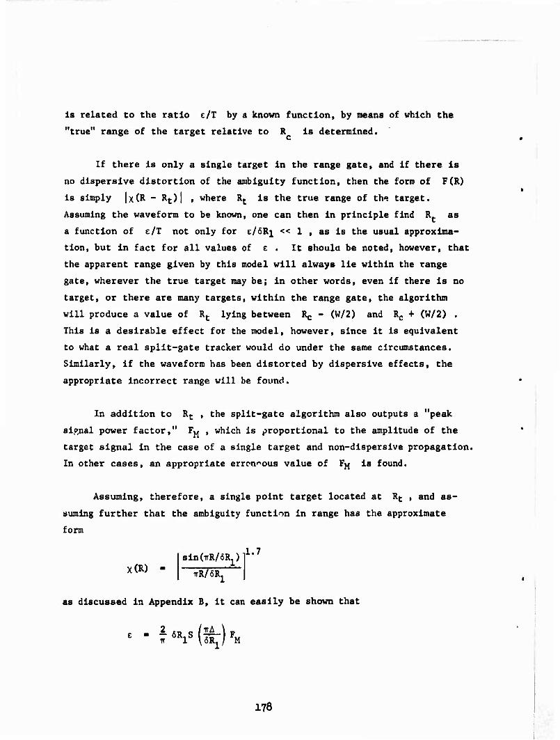
Is related to the ratio c/T by a known function, by means of which the
"true" range of the target relative to R is determined.
If there is only a single target in the range gate, and if there is
no dispersive distortion of the ambiguity function, then the form of F(R)
is simply |x(R - Rt)| > where Rt is the true range of the target.
Assuming the waveform to be known, one can then in principle find Rt as
a function of e/T not only for e/öR^ << 1 , as is the usual approxima-
tion, but In fact for all values of e . It should be noted, however, that
the apparent range given by this model will always lie within the range
gate, wherever the true target may be; in other words, even if there is no
target, or there are many targets, within the range gate, the algorithm
will produce a value of Rt lying between Rj. - (W/2) and Rc + (W/2) .
This is a desirable effect for the model, however, since it is equivalent
to what a real split-gate tracker would do under the same circumstances.
Similarly, if the waveform has been distorted by dispersive effects, the
appropriate incorrect range will be found.
In addition to Rt , the split-gate algorithm also outputs a "peak
signal power factor," Fj^ , which is proportional to the amplitude of the
target signal in the case of a single target and non-dispersive propagation.
In other cases, an appropriate erroneous value of F^j is found.
Assuming, therefore, a single point target located at Rt , and as-
suming further that the ambiguity function in range has the approximate
form
xOO - sinOrR/fiRjT1^
irR/öR.
as discussed in Appendix B, it can easily be shown that
178

imffm*! ■ "H'.iJ.«i||lB!f w-wnw-^
and
T - f 6R1SC:)rM
where x - 7
Since the function S(x) can be tabulated numerically, its inverse,
x = QvS) can also be tabulated. Then if we define
s = S(iT)e/T
the error signal, A , can be found at once using
SRi
whence the target ra-*.ge is given by
The inverse function Q(s) is computed by function QINV (Sec. 4.6.10); it
should be noted that
8ign(A) - slgn(e)
and that if |i| > SOO then |A| = 6^ . The peak power factor, FM ,
is given by
FM " T/[76Ris(lf)J
179

.w 1*1-1 miv - '
The algorithm used In subroutine SPLTGAT for the cases where there
Is only a single ray path between the radar and each real target (N ■ 1)
begins by adding the ln-phase and quadrature components of the returns from
each Interfering target at each point within the range-gate, weighted ac-
cording to the appropriate value of x at tbe given point. Integrating to
find I and I , and then proceeding as described above.
The algorithm used in subroutine MLTSPLT for the case of refraction
through a striated region (N > 1) uses the statistical properties of the
"spread target cloud" as found by subroutine REFRCT to approximate the
video signal envelope which Is Input to the range-tracker. Because of the
statistical nature of this model, ln-phase and quadrature components are
not computed for each target Image; Instead, the random-phase approximation
Is used In comb'nlng the contributions of different Images to the video
signal. See a. the discussion in Appendix E.
•
180

•
APPENDIX E
THE SPREAD TARGET CLOUD 15 THE RADAR BEAM
When the ray path between a target and the radar Intersects a striated
debris region, numerous multiple paths are generated (N > 1), giving rise
to the so-called "spread target cloud" of Images. In ROSCOE, these Images
are described statistically, with the parameters
AR, Au, Av, o&R, c^, o,, y, a, o^
as defined in Appendix G and discussed in Appendix B. For a point target
whose true radar coordinates are (R,u,v), the center of its apparent "cloud"
distribution is at
6R' R1 - R + AR + Ipc -^ (fd - fd)
U. ■ u + Au
v, ■ v + Av
where I_c ■ 1 if the radar Is operating in a pulse-compression mode, and
I - 0 if not. pc
This appendix describes the mathematical modeling of the interaction
between a spread target cloud so defined and a radar beam.
E.l INTERACTION WITH THE RADAR ANGULAR BEAM
In sine-space, the cloud can be represented by an error elLlpse
centered at (u1,v1) with semi-major axis of length a^ and semi-minor
axis of length a2 (these define the one-sigma error ellipse). Its
orientation is defined by stating the angle, y , between the major axis
of the ellipse and the u-axls of the sine-space coordinate system (to
eliminate possible ambiguities, we select 0 <_ y < TT).
181

iw'Simw«««'«"..^''"—-—"^-
The mainlobe of a circular radar bean centered at (u ,v ) can be o o
described by Its one-way relative gain factor
PC '(o . (^)a
as described In Appendix C, Sec. C.l. Here we need only recall that P
is a known constant and
C2 H (u - u )2 + (v - v )2 o o
In order to describe the relation of the cloud error ellipse to the
radar beam pattern, it is convenient to use a rotated set of sine-space
coordinate axes, (u'.v'), which have been rotated about (u ,v ) through
the angle y , so that u1 is parallel to the major axis of the ellipse
and v* Is parallel to the minor axis. Then the new and old coordinates
of any point are related by:
u'-u ■ +(u-u) cos u + (v - v ) sin y o o o
v'-v ■ -(u-u) sin y + (v - v ) cos y 0 0 o
Using this rotated coordinate system, the effective one-way relative
power received from the cloud can be approximated by
00
F(0 /2TÜ
exp ITO,
(u' - u')2
2a? ^Tc exp
ira.
(v' - v')2
2a, du'dv'
provided that a. and a- are sufficiently small that the integrand has
negligible value outside regions where sin x s x .
This integral can be solved by using the exponential approximation
to the function F(0 ; i.e.,
182

|Pppwpyf;!»»BWia;apii|ip,MB|i!iMii, i ^B^^p-»'^^fl»^,^^.-'^J^'^"^• ^^fcmr^T-r-
sin x m e-Ax'
where the constant A can be chosen to force agreement at any particular
point. If the agreement Is to occur at the half-power point, then the
constant is A * 0.1788 . Making use of the fact that
C2 H (u' - u )2 + (v« - v )2 O 0
the double Integral takes the approximate form
Fi ■ 2^r2ffexf\- »»V - V2 + ^ - "o'2^
(u' - uj)2 (v' - vp2 i^«« du'dv
D
This Integral can be solved exactly. The result is
Fl "
where
(Kj + 1) (K2 + 1) -1/2
F(Ö expj- ± 01
uo)2 + ^1 (v' - vo)
2
02 II
K: AAP2a2
KlUo + "i 2
K^ + 1
Vo + Vi K2 + 1
183

-.i.mfiuiwiu i, II,,.,!.,,,,,,,.. -
and
I2 = (G« - urt)2 + (v« - v )2
O 0
The point (u',v') [which can be directly transformed Into the un-
prlmed coordinate system as (u,v)] represents the effective center of the
received power from the target cloud as mediated by the antenna beam pat-
tern. In the same way, £ represents the angle off beam axis (In sine-
space) of the effective center of the spread target cloud, and F^ Is the
effective one-way relative gain factor of the cloud. In this way, we
essentially have reduced the cloud to a fictitious point. The quantities
(R,u,v), |, and F, are computed in subroutine MULTOAR (here R = R.).
E.2 INTERACTION WITH THE AMBIGUITY FUNCTION IN RANGE 2
We have postulated that there are N- target images in the cloud,
with a Gaussian range distribution centered at r ■ R' and having standard
deviation a (which in the present subsection will be renamed a for
notational simplicity). It is assumed that a « R' , and of course 2 r
N_ » 1 . The number distribution of the target Images in the cloud is
NP N(r) - —^ exp
2 r 2
(r - R')2
r
It is further assumed that the mean cross section of the individual
target images in the cloud is a , with standard deviation o . The
total cross section of the entire cloud, if observed as a whole at great 2-
distance, is a_ - N-a .
As before, let XM(' " 'l) be the waveform ambiguity function
(normalised to unity at r - r±) giving the output amplitude at r due
to a unit target at r^ . Thus the amplitude distribution at a point r
due to the target images located around point r. is given by
18U
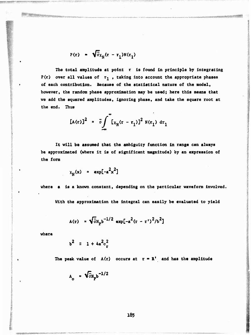
"■HBS^W^ ■
P(r) - V^XN(r - r1)N(r1)
The total amplitude at point r Is found In principle by Integrating
P(r) over all values of r^ , taking Into account the appropriate phases
of each contribution. Because of the statistical nature of the model»
however, the random phase approximation may be used; here this means that
we add the squared amplitudes, ignoring phase, and take the square root at
the end. Thus
[AC
00
•)]2 ■ oj [xN(r - r^]2 NO^) d^
It will be assumed that the ambiguity function In range can always
be approximated (where It Is of significant magnitude) by an expression of
the form
2 2 XN(x)
s exp[-a x ]
where a is a known constant, depending on the particular waveform involved.
With the approximation the Integral can easily be evaluated to yield
A(r) - V^Npb"1/2 exp[-a2(r - r'^/b2]
where
.2 _ ,.22 b I 1 + 4a o
« The peak value of A(r) occurs at r • R1 and has the amplitude
O r
185

'wm"j^finiiin»)«J"J ^ p
This may be Interpreted to mean that the effective range of the cloud
center is at
R = R'
and the effective cross section of the target cloud as mediated by the
ambiguity function of the signal waveform is
oE ■ Np ö/b a -aT/b
Notice that the effective cross section of the target cloud as seen by a
reasonable radar waveform is always less than its ideal total cross section.
For the two kinds of waveforms used in ROSCOE, the value of the para-
meter b will now be calculated.
Simple unchlrped rectangular pulse. The ambiguity function (in range)
for this waveform is shown in Appendix B to be approximated by
XN(x) - expt- 0.884 (2x/ÖR;)2]
whence it is seen that
b2 . i +
Z
»•M (jir) Chirped pulse. The range ambiguity function for the single chirped-
pulse approximation used in ROSCOE was defined in Appendix B to be
% '
sin(irx/6Rp ' i 7
irx/6R|
Making use of the exponential approxiation to the —-— function, the
value of b^' can be computed to be
186
.

pjWi.iH^fflliilW11 ' —^5 ■„mi ij.iimuji^Biiii.^^
b2 • 1 + 12 AkJ E.3 MULTIPLE CLOUDS IN RANGE AND ANGLE
If there Is more than one spread target cloud In the radar range gate, <
and their combined Interference function must be found (as for example in
subroutine MLTSPLT, SLNINTM, and MNOPLSM), the following extension of the
above theory is used.
Suppose there are n overlapping target cloud distributions, all
having the same value of N and or but each ahvlng its own value of
R! and a. . When combining these distributions with respect to the same
radar waveform, we may use the random phase approximation as above, but 2-
modifled so that each individual value of N a. is replaced by the appro-
priately weighted value
-4 Here the.factor (R') takes into account the different ranges of the
2 cloud centers, and (F ) is the relative gain factor (two-way, this time)
to account for the different positions of the clouds with respect to the
antenna beam pattern. Replacing the factor Np\ a in the equation for
A(r) by ^T" , and noting that the exponential exp[-a2(r - r') /b^] in
that equation is merely an approximation to the ambiguity function
XN[(r - R* )/b] , the combined amplitude at point r is given by
A(r) >-11 h k (^ 1-1 L
2^2
187

*•
APPENDIX F
STOCHASTIC REFRACTION MODEL
F.l THIN SCREEN APPROXIMATION
In simulations of radar propagation through a disturbed environ-
ment It Is desirable to be able to determine the statistical descriptors
of the beam as It passes through a medium whose properties vary with
position. The medium will generally have a smoothly varying background
electron density plus an additional fluctuating density which varies much
more rapidly with position. If the fluctuating part of the electron
density does not lead to excessive departures of a ray In the beam from
Its nominal smooth trajectory, It Is possible to develop a theory which
describes, In statistical terms, the effeftts of the electron density
fluctuations.
*
The thin screen approximation provides a description of the
propagation of electromagnetic radiation through an Ionized region of
space, provided the following three conditions are iftet:
1. Ray Optics. The electron density gradients must be suffi-
ciently small that the fractional change in electron density
over distances comparable to a wavelength is small. In
addition, the attenuation over distances comparable to a
wavelength must be small.
2. Straight-Line Approximation. The ray deflections must be
sufficiently small that electron densities and density gra-
dients along the true ray path may be estimated by consider-
ing a nominal straight-line ray path.
189
r«tt« »m BUiMOT nuaB
Jf

3. Small Electron Densities. The electron densities must be
sufficiently small to permit a series expansion in powers
of the electron density.
The name "thin screen approximation" is a slight misnomer
since the basic assumptions may remain valid even though the path length
through the disturbed region Is fairly long. However, for a given angu-
lar deflection there Is s limiting path length beyond which the straight-
line approximation breaks down.
We consider a region with a magnetic field in the z-dlrectlon
and an electron density n (x,y) which Is Independent of z . In the ct
absence of the electrons, a wave packet of radiation moven In a straight
line with the speed of light, and we choose our coordinate system so that
the nominal ray lies In the x , z-plane, making an angle Y with the
z-axls.
The electric field then has the form
E - E exp(iki|) sin y + Ikz cos Y - lut)
- E0 exp(l* - lut)
where 41 Is a function only of x and y , satisfying the equation
(V*)' - 1 - -l-o. ncr sin Y
according to the ray optics approximation. Here n Is the critical
electron density at the frequency f , and k - 2ir/X . This equation
determines the electric field at an arbitrary point In space If the
value of i|i Is known on the plane x - x If the electron densities
are sufficiently small, \|» may be expanded In powers of o so that
190
■

W^WWWWWW""
* " ^o + *1 + ^2 + "*
On the surface x - x , i|)(x ,y) • x + ^(x ,y) , where ^ is assumed to
be a first-order quantity. We therefore take ij; (x,y) ■ x , and this des-
cribes the nominal straight-line path.
The the first-order corrections to i|» are determined by
ro rl e
so that
3«j
äx" i
-20e
and
^(x.y) - i|»(xo,y) - 2 J v^ *y} dxl
Similarly, the second-order terms give
3^ 2_i..(7V».. !(,»).,!
where
e - Nu 37
is the angle that the projection of the ray path onto the x,y-plane makes
with the x-axis (to first order). Thus
191
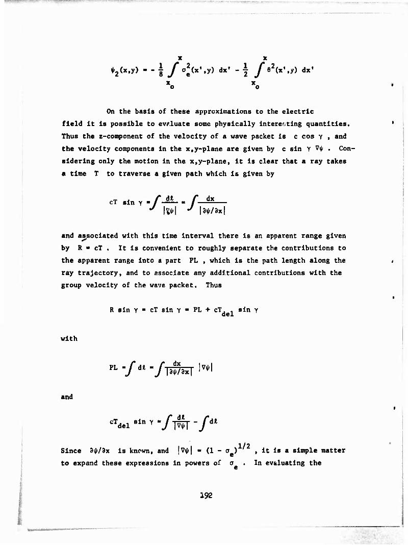
.Il^l». jui ir.-"-.-,-,-,--™^,JsWW,.Wj,„v.,, - - ^^^^rrrrrr^rr*,-*,.-
♦2(x,y) m-\ /0l^,y) a*' -j f*2(*',y) dx' o o
On the basis of these approximations to the electric
field It Is possible to evaluate some physically Interesting quantities.
Thus the z-component of the velocity of a wave packet Is c cos y , and
the velocity components In the x,y-plane are given by c sin Y '♦ • Con-
sidering only the motion In the x,y-plane. It Is clear that a ray takes
a time T to traverse a given path which Is given by
cT sin Y - / ■ /
and associated with this time Interval there Is an apparent range given
by R = cT . It Is convenient to roughly separate the contributions to
the apparent range Into a part PL , which is the path length along the
ray trajectory, and to associate any additional contributions with the
group velocity of the wave packet. Thus
R sin Y ■ cT sin Y ■ PL + cT 1 sin Y
with
dx n-/il ■ fwm'"*' and
'fwcf1 cTdel 8ln Y - / T^TT - / d*
1/2 Since 3iJ»/3x is known, and \Vty\ - (1 - o ) , it is a simple matter
to expand these expressions in powers of o . In evaluating the
192

expressions obtained, It must be remembered that y varies with x along
a ray trajectory so that
dx Wax
The results of such an expansion are
PL " « - xo + rdl
where the "dogleg" range error Is given by
rdl | J eV.y«) dx«
and
cTdel 8ln Y "i / «V«'»^ dx, +1 / ^^'»y^ dx,
so that the apparent range for a ray going from x to x Is
R - x - x + r.,, + cT, b sin Y dl del
In applications, the second-order contribution to T. . Is
gtr.crally negligible compared to the first-order term, and nay be Ignored.
However, because of geometric factors, the dogleg term r... can be ap-
preciable, and should be retained.
193

The phase of a ray moving through the medium changes so that
6* - k sin Y '«I» + k cos y **
- k sin Y |^| <U + k cos2 Y 5T
since In the x,y-plane 6r - V^££/|Vi|;| . It Is then easily seen that the
phase change In moving from x to x Is given by
A* - kR - 2kcTdel sin2 Y
In deriving the last equation, an approximation has hern made In that some
liberties were taken with the second-order contrlbutlonü to T, ,. del
F.2 STOCHASTIC REFRACTION MODEL
(U) In the last section an approximate expression for the electric
field was obtained In terms of the electron density distribution. In
practice the electron density function is often not known in detail but
must be described in statistical terms. We therefore consider a model in
which the electron density fluctuations are due to field aligned stria-
tions so that
(x - xk) + (y - yk)
where the location of the strlation axes (xk.y,), the peak electron den-
sity of the strlation v n and the strlation size a. are not known
precisely. Instead we assume (x. »Yj) are randomly distributed in the x,y-
plane with a two-dimensional density function p(x) , that v. and a.
<vV2> are also randomly distributed, and that the average moments
are known as functions of x . It is then desired to calculate the expected
value of various physically interesting quantities; this is done in the
following subsections.
19^
,

F.2.1 Integrated Electron Density
The quantity
/n (x'.y) dx' -Z-
r cr
Is linearly related to the absorption due to electron-neutral collisions
and is also useful In that several other quantities are readily calcu-
lated once d is known. When a ray passes the kth striation there is a
contribution to d(x,y) given by*
CO
dk(y) - vk exP[-(y - yk)2/aj] / exp(-x2/aj;) dx
1/2 i , ,2 [-(y - y,)2/^]
and
d(x,y) f vCx') dx' + ^ dj
where the sum over J extends over all strlations in the region
x < x. < x and -» < y < •. o J J
The average contribution of those strlations in the Interval
from x1 to x' + dx can be obtained by replacing the sum over j by
an integral over the possible positions of the striation centers so that
(U) The use of the limits -•> to +«> for the x-integration is justi- fied by the assumption that a. is small compared to other scale sizes of the problem.
195

2 djCy)^ - PU") dx • //.(.^V^'V
where the expectation value under the integral sign is an average
over the distribution in v and a . Thus
» x
D(x) - ^d(x.y)^ - J v(x') dx' + ir y pCx'^va2^ dx'
o o
F.2.2 Fluctuations in Integrated Electron Density
Consider
2
dU.y) - f vCx«) dx'j - 2 V50 S dj(y> / i i
As before the average value of this quantity may be obtained by replacing
the sums by Integrals. However, the terms with 1 B J must be considered
separately since they also give rise to a finite contribution. Thus
Sd^y) 2 djCy) "I" J P(x,)Wa2> dx'
2, 2 + / dx' Pfr')//' v2a2ire'2y /a dy
196

where the second term on the right-hand side comes from the
terms with i - j . Thus the fluctuations in d(x,y) are given by
»*(x) -( [d(x, y) - D(x) > 2 J/2 r / PU'XVV >d>t4
F.2.3 Emergence Angle
Each striation scatters the ray through an angle
9 . V172» - rt)
\ sin Y 2 exp|" (y - yk)2/\
so that the ray makes an angle with the x-dlrection given by
e(x) - Z^ e
which is easily seen to have zero expectation value. The square of this
angle has expectation value
OQ(X) -(e2(x)V(iCS £?.;.:>-<?<* and replacing the sum by an integral gives the result
.jw /
de_ dx r dx*
197

with
£-li)"'T±r.'"<■■■) .2 /^3/2 1 /,\ *
I 2 sin Y
F.2.A Miss Distance
A ray will suffer a displacement In the y-dlrectlon given by
Äy(x) - E (x- \)*l
which has zero mean. The expected value of Its square Is readily found
and
aAy(x> " \hx)l Z" / (X " X,)2 ^ dx, x o
F.2.5 Range Error
A ray in propagating from the kth to the k + 1th striatlon
makes an angle 6. with the x-axls given by
"k - E o- j-i ]
and the distance It must travel exceeds the nominal distance x.+. - x^
by an amount (1/2) (x... - »O^t • Thu8 in traversing «-.he medium there
la a "dogleg" range error given by
rdl " I £ (xk+l " V6
196

I
which has expectation value
»di - T / •?<»•> *■• - i / <« * «'> 3^ <*' X X o o
The total range error consists of this tern plus a time delay term
R - ~— R.. + cT. . e sin Y dl del
where
cT • , W— D del 2 sin3 Y
F.2.6 Range Fluctuations
Consider first
'dl ■ ? 2 CV» - V8» Z «Vl " "n"
It Is easily seen that the terms with m ■> n give a vanishing contrlbu- 2 tlon to the expectation value of r.. so that It Is sufficient to con-
sider n. > m and multiply by 2. For n > m ,
eV }'< n m.
n n m m
E Z E L •I'M«: i-1 j-1 k-1 t'l
4 wfa+ 2[0fa\z + 2«(x ) m
199

mmmmm
where the first tern cones fron 1 - J, k - I , and the next tern cones
from 1 - k, j - t , and 1 - t, j - k contributions, and i - J - k - 1
gives rise to
♦c-i(z: (.;,)-^),/,^r-/.<..^.>fc.
SO
o2dlM - /* (X - K>)||o|(x,)| + *(x')| dx'
The cross correlation between the dogleg and line delay terns is gi-'en by
ctdelrdi; - cTdelRdl
k 2
4
1
Bin Y E
k (Vi -v
J-l V*?
3 '2G) 3/2
(
1 X
/ Xo
(x - XOPU' 16 .in8 Y
and
2 12 2
e 4 sin Y e
200

F.2.7 Beam DefocuBsing
Consider two rays which initially make angles with the x-axis
which differ by AO . After propagating through the medium, two such
rays will be separated by a distance
«y(x) - xAeo + £(x - \) ^ Ö^V
The sum over k has zero expectation so that it is necessary to consider
(6y) • (Note that tyOO and de"/3y trt statistically independent.)
If we let S(x) -(P^l > then
,3/2
<W"> S(x) - x2 +|(y) —ij— y (x - x^^Cx'^vV^SCx') dx'
Yx o
However, because of the presence of S on the right-hand side the final
result for S involves an expansion containing all powers of the peak
electron density. Since in the underlying theory all powers of the peak
electron density higher than the second have been ignored, these higher
prder suns in S are not reliable. Therefore, in applications it is 2
prudent to replace S by its "Born approximation" S(x) - x when it
occurs under the integral sign.
The gain G due to focussing is then
G(x) - [x2/S(x)l1/2
It must be emphasized at this point that the gain (always less
than unity) given by this equation is absociated with a single ray path
connecting the radar to the target. In general, there may be many such
201

one-way Images and the total energy on the target contains a factor N.G ,
If the radar beamwldth is sufficiently large, it can be argued that N G
is on the average equal to 1. The energy in the beam sweeps through any
region of space on the average N. times at the range considered. If it
is assumed the electric fields associated with different rays are inco-
herent, then the energies associated with different rays add and energy
conservation demands that N.G ■ 1 . The angular separation between rays
at the radar associated with successive images can also be estimated.
As before, denote the miss distance by Ay . During an angular interval
such that jg > 0 a ray will pass through an interval of angle such that
Ay starts at a negative minimum, hits the target, and then rises to a
local maximum. If the root mean squared angle traversed in going from a
minimum to a maximum is A6. then
Ae1 - 2 üU£L
m) 1/2
>&
- 2 VG
Thus if the antenna beamwldth is Y then the number of images is
JJL 2oA G Ay
and the energy incident on the target is multiplied by a factor
(Yx)/(2ojy).
The treatment developed above has some advantages over previous
formulations. In the past, expressions for the dogleg range error, its
scintillation, and the focussing gain have been obtained by heuristic
202

arguments. The formulas for this paper have been derived more systematically
and to the extent that the underlying thin screen assumptions are valid they
are correct. If there are several targets In a radar beam It Is possible,
using the present formulation, to Integrate up to the first target and then
simply continue on to the next target. In the older formulations It was
necessary to redo the entire calculation for each new target.
203

APPENDIX G
DEFINITIONS OF SYMBOLS
Underlined terms are lists in the sense explained In Vol. 1. An
asterisk (*) denotes an Input parameter. A double asterisk (**) denotes
a precomputed quantity derived from Input parameters stored in some dataset.
**
Dispersion constant ujed in subroutine REF1S, -3/2
n o A^ - 0.0828 B £
A^ Dispersion parameter defined In REF1S
l A-,A ,A Constants relating to the standard deviations of the K U V
radar measurement errors; these give the signal-to-
noise-independent term in the respective expressions
A Multiplying factor used In POSSV, POSLIST to Include
possible interfering targets within a specified angle
of the desired target
B Effective signal bandwidth
B Noise bandwidth, B ■ 1/(pulse duration)
BR,B ,B Constants relating to the standard deviations of the
radar measurement errors; these are used to find the
signal-to-noise-dependent term in the respective ex-
pressions
C Total received clutter power from fireballs and dust
clouds
205

Slope of the angle sldelobe taper (not currently
used)
M, Symbols used interchangeably for the radar transmitted
center frequency
F.F, Symbols used Interchangeably for the one-way relative
gain due to off-axis position of the target in the radar
beam
pc
L
Pulse compression ratio for the given waveform
Expected doppler shift, to whi-h the receiver filter
is matched
Ad
FM.FMAX
Actual doppler shift for a given target
Symbols used interchangeably for the amplitude factor
from which the output signal power can be computed
ILg- Altitude below which it is assumed that no refraction
takes place (used in REF1S)
IL^ Current altitude of the radar (used in REF1S)
2 1- Integrated electron density (electrons/cm ) along the
path to the target (computed in REFRCT)
IFAIL Integer index of success or failure of threshold cros-
sing (see RAD1S, etc.)
IFDET Integer index output by RADMODS; IFDET - 0 indicates
that no detection has occurred
206

ITO Serial number In POSLST of the target of Interest
(computed In RAD1S)
L Dispersive loss factor (computed In DISPERS)
LF Faraday rotation loss factor (computed In REF1S)
L- Two-way path absorption to the target point (computed
In ABSORB)
oro A maximum absorption parameter (computed In RAD1S)
LISTA.LISTS Lists of: Interfering targets (see Sec. 4.4.5)
i
MLST Number of targets In LISTA or LISTB (computed In REFLST1
or REFLSTN)
MGRP List of targets In mutually unresolvable groups (com-
puted In REFLST1)
NLST Number of targets In list POSLST
NGRPS Number of close-target groups In LISTA (see REFLST1)
I **N Nominal system noise power. N - kB T
' ' • n n n
Number of direct propagation paths between radar and
target (computed In REFRCT)
i NT Identification number of the target of current Interest
(used in POSLIST and POSSV)
** Beamwidth factor (see GOA, etc.), p - 1.392/äw
207

POSLST Possible-targets list; see Sec. 4.2.3
* 2 R Range at which aim target will Just exceed threshold
R Range to the center of the receive range gate
R Range to a given target point
R. Range to the particular target point defined in RAD1S
R Range to the apparent center of the "spread target
cloud" in the striated case (see MULTOAR)
R* Apparent target range (an ultimate output)
R' Apparent target range when used as an input to the
monopulse routines MNOPLS and MNOPLSM
RMAX Range to the highest output peak in SVPEAKS
o
**
So - (S/N>TiRoNn
S Revised parameter used in computing received signal
power; after REF1S it has the value
s, - s C082 1 1 o L2LDLF
20B
i
R Additive range used in POSLIST to include possible
interfering targets within 3000 feet of the range
gate
** S Parameter used in computing received signal power,
■'•

It S One-way angular sidelobe (power) level, relative to
p
s unity on the beam axis at boreslght (the near-ln value
I for tapered sidelobe model)
S Constant range sidelobe (power) level, relative to oh
( unity at the peak of the undlspersed ambiguity function,
for chirped pulses (used in AMBGN)
(S/N) . Pre-detectlon signal-to-noise threshold for the given
r
I
'Ti event and waveform
Parameter used in split-gate range tracking (see
SPLTGAT, MLTSPLT, and QINV)
Time of the current event
* T Effective receiver temperature
T System reference temperature, T - 290oK
T Nominal system noise temperature, T - T + T
T Total effective outside noise temperature
(u,v) Sine-space coordinates of a given target point
(u ,v ) Sine-space coordinates of the current radar-beam axis o o
(u,^j) Sine-space coordinates of the particular target point
defined in RAD1S
(u,v) Sine-space coordinates of the apparent center of the
"spread target cloud" In the striated case (see MULTOAR)
209

(u'.v*) Apparent target sine-space coordinates (an ultimate
output)
V Current value of the width of the receive gate
■ X Total noise plus clutter power
Y Trial signal-to-noise ratio which is compared with
L to see if a threshold crossing is possible, in om RAD1S and REF1S
Z Signal-to-noise-plus-clutter ratio at the output of
the receiver filter (an ultimate output)
a Safety factor used in RAD1S (see Sec. 4.3.1)
AR Refractive range bias error (see Appendix B) t
(AA.AE) Refractive angular bias errors when N ■ 1 (see
Appendix B) ")
(Au.Av) Refractive sine-space bias errors to center of "spread
target cloud" when N > 1 (see Appendix B)
AX- Equivalent noise increment due to range sidelobe target
interference
** 6R Nominal range-resolution width for unchlrped pulse,
o 6R ■ CT/2 t
o *
* 6R. Radar bias error in the range coordinate
210
.

*
** 6R- Nominal range-resolution width for a chirped pulse,
6R. = 2ÖR /F 1 o pc
OR',OR' Dispersion-distorted range resolution widths,
6R; = LD6Ro and ÖRj - L^
6u, ,6v. Radar bias errors in the u,v coordinates
6w One-way, 3-dB half-beamwldth in sine-space,
6w - sin(66/2)
66 One-way, 3-dB angular beamwidth at boreslght
6 Angle off boreslght of radar beam axis (computed in
RAD1S), cos 6 - (l - u2 - v2)1/2
y Slope-angle in sine-space of the "spread target error
ellipse," relative to the u-axls (see Appendix B)
C Angle off beam axis in sine-space for a given target,
5 - [u - uo) + (v - vo) ]
I Angle off beam axis in sine-space of the apparent
center of the "spread target cloud" in the striated
case (see MULTOAR)
a Standard deviation of the refractive range bias error
(aAAtOAE) Standard deviations of the refractive angular bias
errors when N ■ 1 (see Appendix B)
(a. ,o2) Semi-major and semi-minor axes, respectively, of the
sine-space error ellipse in the "spread target" case
(see Appendix B)
211

Mean cross section of the Individual targets In the
"spread target cloud" for the striated case
a Standard deviation of the distribution (about o) of
the Individual "spread target" cross sections
XN Waveform ambiguity function normalised to unity at Iti
peak (see AMBGN). For chirped pulses, its argument
already contains an adjustment due to range-doppler
coupling (see REFLST1 and MULTOAR)
ftp Faraday rotation angle (where applicable; see REF1S)
T Pulse duration
212
i
)

ÜMnamwa
DISTRIBUTION LIST
DEPAHTMENT OF DEFENSE DEPARTMENT OF THE ARMY (Continued)
Director Command Control Technical Center
A TIN: C312, Italph Mason
Director Defense Advanced Rsch ProJ Agency
ATTN: Strategic Tech Office
Defense Communication Engineer Center ATTN: Code IM 10, James W. McLean
Director Defence Communications Agency
ATTN: Code 480
Defense Documentation Center 12 cy ATTN; TC
Director Defense Nuclear Agency
ATTN: DD8T ATTN: STSI, Archives ATTN: RAAE
ScyATTN: STTL, Toch library
Commander Field Command, DNA
ATTN: FCPR
Commander Harry Diamond Laboratories
ATTN: ORXDO-NP. Franc!» N. WimeniU ATTN: DRXDO-TI. library
Commander TRA8ANA 2cyA1TN: R. E. Dekinder, Jr.
Director U. 8. Army Ballistic Research Labs
ATTN: MarkD. Krr-el ATTN: Lawrence J. .»uckett
Commander, U.S. Army Foreign .Science I Tech Ctr
ATTN: P. A. Crowley ATTN: R. Jones
Commander U.S. Army Missile Command
ATTN: DRSMI-XS, Chief Scientist
Commander U.S. Army Nuclear Agency
ATTN: W. J. Berberet, ATCA-NAW
DEPARTMENT OF THE NAVY
Director Interservice Nuclear Weapons School
ATTN: Document Control
Director Joint Strat Tgt Planning Staff. JCS
ATTN: JPST, Capt D. GoeU
Chief Uvermore Division, FC, DNA Lawrence Uvermore Laboratory
ATTN: FCPRL
OJCS/J.3 ATTN: J-3 WWMCCS, Mr. Toma
DEPARTMENT OF THE ARMY
Commander/Director Atmosph» 'Ic Sciences Laboratory U.S. Army Electronics Command
ATTN: DRSEL-BL-SY, F. E. NUes
Director BMD Advanced Tech Ctr Huntavllle Office
ATTN: CRDABH-O, W. Davies ATTN: ATC-T, Melvin T. Capp»
Program Manager BMD Program Office
ATTN: John Shea ATTN: Plans Division ATTN: DACS-BMS, Julian Davidson
Chief of Naval Operations Navy Department
ATTN: Alexander Brandt ATTN: Ronald E. Pitkin
Commander Naval Electronics Laboratory Center 3 oyATTN: Code 2200, Verne E. Hildebrand
Director Naval Research Laboratory
ATTN: Code 7701, Jack D. Brown ATTN: Code 2027, Tech Library ATTN: Code 7700, Timothy P. Cotfey ATTN: Code 7760, 8. Ossakow
Commander Navel Surface Weapons Center
ATTN: Code WA501, Navy Nuc Prgms Off ATTN: Code WX21, Tech Library
Director Strategic Systems Project Office Navy Department
ATTN: NSP-2722, Marcus Meaerole
DEPARTMENT OF THE AIR FORCE
AF Geophysics Laboratory, AFSC ATTN: OPR, James C. Ulwlck ATTN: OPR. Alva T. Stair ATTN: OPR, Harold Gardiner
213

DEPARTMENT OF THE Al« FOHCE (Continued)
AF Weapons Laboratory, AFSC ATTN: UYT Peter W Lunn ATTN: CA, Arthur H. Uuenther ATTN: SUL ATTN; SAS. John M. Kamm ATTN: DYT Capt Mark A. Fry
AFTAC ATTN: TF, Maj Wiley ATTN: TN
HQ USAF/RD ATTN: RDQ
DEPARTMENT OF DEFENSE CONTRACTORS (Continued)
Commander Rome Air Development Center, AFSC
ATTN: EMTLD Doc Library ATTN: V. Coyne
SAMSO/MN ATTN: MNX
SAMSO/SZ ATTN: SZJ, Maj Lawrence Doan
Commander In Chief Strategic Air Command
ATTN: XPFS, Maj Brian G. Stephan
ENERGY RESEARCH t DEVELOPMENT ADMINISTRATION
University of California Lawrence Livermore Laboratory
ATTN: Ralph S. Hager, L-31 ATTN: Donald R. Dunn, L-156
Los Alamos Scientific Laboratory ATTN: Doc Con for John Zinn ATTN: Doc Con for Eric Jones
Sandia Laboratories ATTN: Doc Con for J. C. Eckhardt, Org 1250 ATTN: Doc Con for 3141, Sandia Rpt Coll ATTN: Doc Con for W. D. Brown ATTN: Doc Con for Charles Williams
OTHER GOVERNMENT AGENCIES
Department of Commerce Office of Telecommunications Institute for Telecom Science
ATTN: William F. Utlaut
DEPARTMENT OF DEFENSE CONTRACTORS
Aerospace Corporation ATTN: Norman D. Stockwell
Brown Engineering Company, Inc. ATTN: Joel D. Blgley
Calspan Corporation ATTN: Romeo A. Deliberls
ESL, Inc. ATTN ATTN ATTN
R. K. Stevens James Marshall V. L. Mower
General Electric Company TEMPO-Center for Advanced Studies
ATTN: Tim Stephens ATTN: WarrenS. Knapp ATTN: DASIAC
General Research Corporation ATTN: John Ise, Jr. ATTN: John Boys ATTN: JoeGabaring
Johns Hopkins University Applied Physics Laboratory
ATTN: Document Librarian
Lockheed Missiles t Space Co., Inc. ATTN: D. R. Churchill
M.I.T. Lincoln Laboratory ATTN: Lib A-082 for David M. Towle
Martin Marietta Aerospace Orlando Division
ATTN: Roy W. Heffner
Mission Research Corporation ATTN: Dave Sowie ATTN: W. F. Crevier ATTN: Paul Fisher ATTN: Roy Hendrick ATTN: Russell Christian
Physical Dynamics, Inc. ATTN: Joseph B. Workman
Science Applications, Inc. ATTN ATTN ATTN
D. Sachs Raymond C. Lee Curtis A. Smith
Science ^Pflications, Inc. HuntsvHe Di tfsion
ATTN: Nuel R. Byrn ATWts Dale Divis
Stanford at * jarch Institute ATI?!: Jacqueline Owen ATTN: Walter G. Chesnut
Visldyne, Inc. ATTN- J. W. Carpenter ATTN: Henry J. Smith ATTN: Chuck H. Humphrey
I
ZLk