© pearson education, 2005 basics of macroeconomics and the aggregate supply and aggregate demand...
Post on 20-Dec-2015
214 views
TRANSCRIPT

© Pearson Education, 2005
Basics of Macroeconomics and the Aggregate Supply and Aggregate Demand Model.
Topic 9

© Pearson Education, 2005
Objectives
After studying this topic, you will able toDescribe the origins of macroeconomics and the problems with which it deals
Describe the trends and fluctuations in economic growth
Describe the trends and fluctuations in unemployment
Describe the trends and fluctuations in inflation
Describe the trends and fluctuations in government and international deficits
Identify the macroeconomic policy challenges and describe the tools available for meeting them
Define GDP and use the circular flow model to explain why GDP equals aggregate expenditure and aggregate income
Explain two ways of measuring GDP
Explain how we measure economic growth, real GDP and the GDP deflator
Explain how real GDP is used as an indicator of economic welfare and describe its limitations
Explain what determines aggregate supply
Explain what determines aggregate demand
Explain macroeconomic equilibrium and the effects of changes in aggregate supply and aggregate demand on economic growth, inflation and the business cycle
Explain UK economic growth, inflation and business cycles by using the AS-AD model.
Explain the main schools of thought in macroeconomics today

© Pearson Education, 2005
Economic Growth in the United KingdomThis figure shows real GDP in the United Kingdom from 1963 to 2003.
The figure highlights:
• Fluctuations of real GDP• Smoother growth of potential GDP• During the 1970s and early 1980s, real GDP growth slowed—a productivity growth slowdown.
Economic Growth
© Pearson Education, 2005
Every business cycle has two phases:
1. A recession is a period during which real GDP decreases for at least two successive quarters.
2. An expansion is a period during which real GDP increases.
and two turning points:
1. A peak
2. A trough
Economic Growth

© Pearson Education, 2005
This figure shows the most recent UK cycle.
Economic Growth

© Pearson Education, 2005
Economic Growth
This figure shows the UK cycles over the past 150 years.
© Pearson Education, 2005
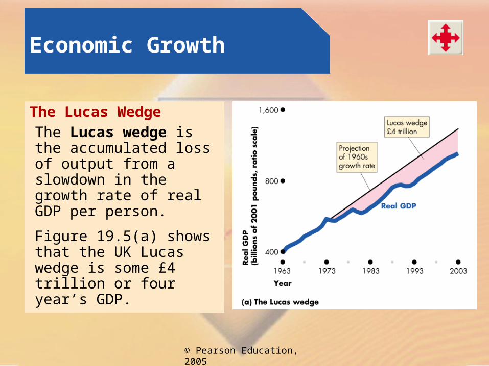
The Lucas WedgeThe Lucas wedge is the accumulated loss of output from a slowdown in the growth rate of real GDP per person.
Figure 19.5(a) shows that the UK Lucas wedge is some £4 trillion or four year’s GDP.
Economic Growth

© Pearson Education, 2005
The Okun GapThe Okun gap is the gap between potential GDP and actual real GDP and is another name for the output gap.
Figure 19.5(b) shows that the Okun gaps since 1973 are £98 billion or about 5 week’s real GDP.
Economic Growth
© Pearson Education, 2005
Unemployment
Unemployment is a state in which a person does not have a job but is available for work, willing to work, and has made some effort to find work within the previous four weeks.
The workforce is the total number of people who are employed and unemployed.
The unemployment rate is the percentage of the people in the workforce who are unemployed.
A discouraged worker is a person who available for work, willing to work, but who has given up the effort to find work.
Jobs and Unemployment
© Pearson Education, 2005
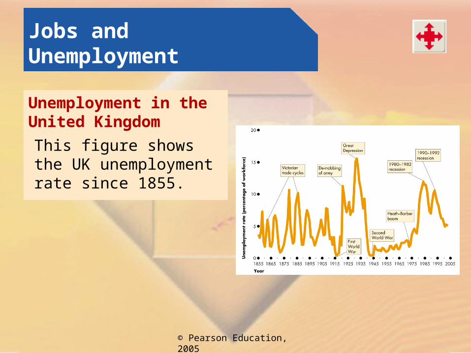
Unemployment in the United Kingdom
This figure shows the UK unemployment rate since 1855.
Jobs and Unemployment

© Pearson Education, 2005
Inflation is a process of rising prices.
We measure the inflation rate as the percentage change in the average level of prices or price level.
The Retail Prices Index—the RPI—is a common measure of the price level.
Inflation
© Pearson Education, 2005
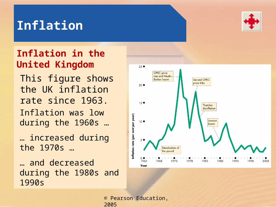
Inflation in the United Kingdom
This figure shows the UK inflation rate since 1963.
Inflation
Inflation was low during the 1960s …
… increased during the 1970s …
… and decreased during the 1980s and 1990s
© Pearson Education, 2005
Government Budget Surplus and Deficit
If a government collects more in taxes than it spends, it has a government budget surplus.
If a government spends more than it collects in taxes, it has a government budget deficit.
Surpluses and Deficits

© Pearson Education, 2005
This figure shows the changing surplus and deficit of the UK government since 1973.
The government budget has had persistent deficits and only rarely been in surplus during these years.
Surpluses and Deficits
© Pearson Education, 2005
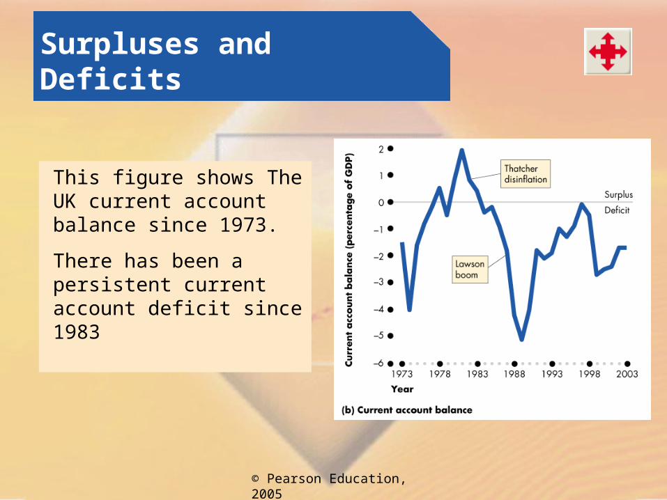
This figure shows The UK current account balance since 1973.
There has been a persistent current account deficit since 1983
Surpluses and Deficits

© Pearson Education, 2005
Five widely agreed policy challenges for macroeconomics are to:
1. Boost economic growth
2. Stabilize the business cycle
3. Lower unemployment
4. Keep inflation low
5. Reduce government and international deficits
Macroeconomic Policy Challenges and Tools

© Pearson Education, 2005
Gross Domestic Product
GDP Defined
GDP or gross domestic product, is the market value of all final goods and services produced in a country in a given time period.
© Pearson Education, 2005
Gross Domestic Product
This definition has four parts:
Market Value
GDP is a market value goods and services are valued at their market prices.
Final Goods and Services
GDP is the value of the final goods and services produced. A final good (or service) is an item bought by its final user during a specified time period.
Produced Within a Country
GDP measures production within a country domestic production.
In a Given Time Period
GDP measures production during a specific time period Excluding intermediate goods and services avoids double counting normally a year or a quarter of a year.
© Pearson Education, 2005
Gross Domestic Product
GDP and the Circular Flow of Expenditure and Income
GDP measures the value of production, which also equals total expenditure on final goods and total income.
The equality of income and output shows the link between productivity and living standards.
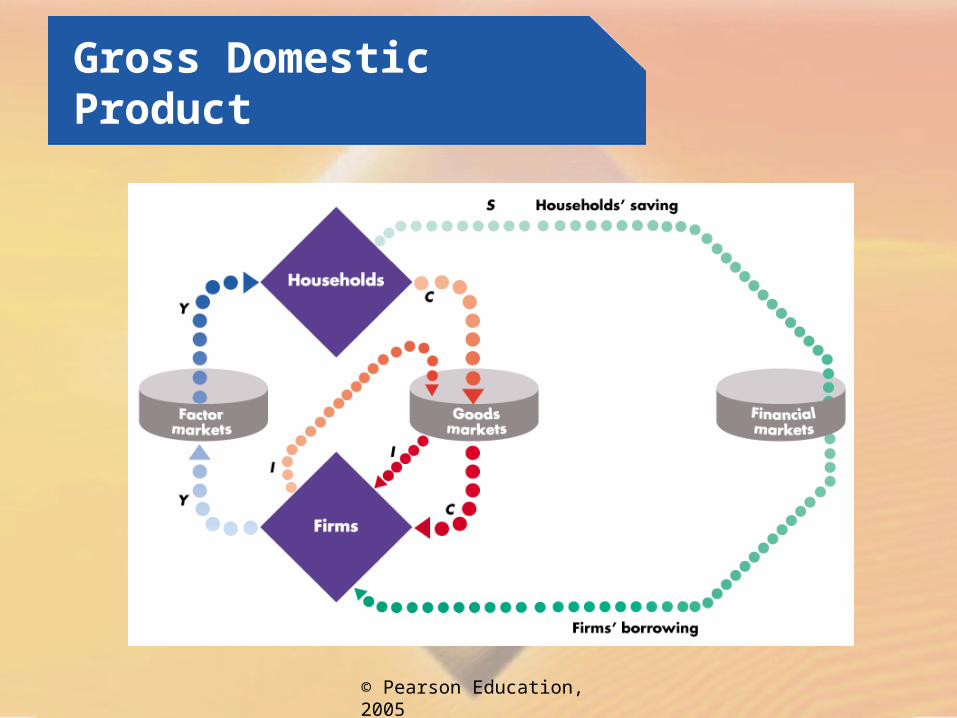
Figure 20.1 illustrates the circular flow of expenditure and income.
© Pearson Education, 2005
Gross Domestic Product
© Pearson Education, 2005
Gross Domestic Product
© Pearson Education, 2005
Gross Domestic Product

© Pearson Education, 2005
Gross Domestic Product
GDP Equals Expenditure Equals Income
The circular flow demonstrates how GDP can be measured in two ways: by total expenditure or by total income.
Total expenditure on final goods and services equals the value of final goods and services, which is GDP.
Aggregate income earned from production of final goods, Y, equals the total amount paid for the use of resources: wages, interest, rent and profit.
Total expenditure = C + I + G + (X – M)=Y (Income).

© Pearson Education, 2005
Gross Domestic Product
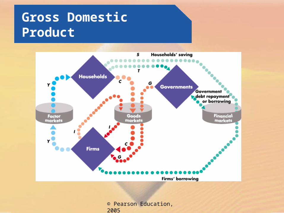
Financial FlowsFinancial markets finance deficits and investment.
Household saving, S, is the income minus net taxes and consumption expenditure.
Y = C + S + T
(A) Saving flows from households to the financial markets
[S].
(B) If government expenditures exceed net taxes, the deficit [G – T] is borrowed from the financial markets (if T exceeds G, the government surplus flows to the financial markets).
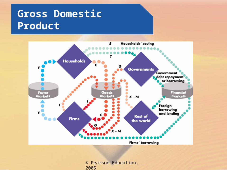
(C) If imports exceed exports, the deficit with the rest of the world [M – X] is borrowing from the rest of the world.

© Pearson Education, 2005
Gross Domestic Product
How Investment Is FinancedWe can see these three sources of investment finance by starting with the fact that aggregate expenditure equals aggregate income.
Y = C + S + T = C + I + G + (X – M).
Then rearrange to obtain
I = S + (T – G) + (M – X)
Private saving S plus government saving (T – G) is called national saving.

© Pearson Education, 2005
Gross Domestic Product
Gross and Net Domestic Product“Gross” means before accounting for the depreciation of capital. The opposite of gross is net.
To understand this distinction, we need to distinguish between flows and stocks.
Flows and Stocks in Macroeconomics
A flow is a quantity per unit of time; a stock is the quantity that exists at a point in time.
e.g. Wealth, the value of all the things that people own, is a stock. Saving is the flow that changes the stock of wealth.

© Pearson Education, 2005
Gross Domestic Product
Capital and Investment
Capital, the plant, equipment, and inventories of raw and semi-finished materials that are used to produce other goods and services is a stock. Investment is the flow that changes the stock of capital.
Depreciation is the decrease in the stock of capital that results from wear and tear and obsolescence.
Gross investment is the total amount spent on purchases of new capital and on replacing depreciated capital.
Net investment is the change in the stock of capital (= Gross investment Depreciation).

© Pearson Education, 2005
Gross Domestic Product
This figure illustrates the relationships among the stock of capital, gross investment, depreciation and net investment.

© Pearson Education, 2005
Measuring UK GDP
The Office for National Statistics uses the concepts that you met in the circular flow to measure GDP and its components, which are published in the United Kingdom National Accounts.
Two approaches to measuring GDP are:
The expenditure approach The income approach

© Pearson Education, 2005
Measuring UK GDP
The Expenditure Approach
The expenditure approach measures GDP as the sum of consumption expenditure, investment, government expenditures on goods and services and net exports.
The Income Approach
The income approach measures GDP by summing the incomes that firms pay households for the factors of production they hire.
© Pearson Education, 2005
Measuring UK GDP
The Income ApproachIn the United Kingdom National Accounts, incomes are divided into three categories
1. Compensation of employees2. Gross operating surplus3. Mixed incomes
The sum of these three income components is gross domestic income at factor cost.
GDP is gross domestic product at market prices.
Market prices and factor cost would be the same except for indirect taxes and subsidies.
To get from factor cost to market prices, we add indirect taxes and subtract subsidies.

© Pearson Education, 2005
Real GDP is the value of final goods and services produced in a given year when valued at constant prices.
The first step in calculating real GDP is to calculate nominal GDP.
Nominal GDP
Nominal GDP is the value of goods and services produced during a given year valued at the prices that prevailed in that same year.
Measuring Economic Growth

© Pearson Education, 2005
The table provides data for 2002 and 2003.
(A) 2002, nominal GDP is:
Expenditure on balls £100
Expenditure on bats £100
Nominal GDP £200
(B) 2003, nominal GDP is:
Expenditure on balls £80
Expenditure on bats £495
Nominal GDP £575
Item Quantity Price
2002
Balls 100 £1.00
Bats 20 £5.00
2003
Balls 160 £0.50
Bats 22 £22.50
Measuring Economic Growth

© Pearson Education, 2005
Nominal GDP was £200 in 2002 and £575 in 2003, so nominal GDP increased by £375.
The percentage increase in nominal GDP was (£375/£200) 100 = 187.5 per cent.
How much of this 187.5 per cent increase is an increase in production and how much is just the effect of higher prices?
The answer is found by valuing the 2003 quantities at 2002 prices.
Measuring Economic Growth

© Pearson Education, 2005
Current-year Production at Previous-year Prices
Expenditure on balls in 2003 valued at 2002 prices is £160.
Expenditure on bats in 2003 valued at 2002 prices is $110.
Value of 2003 quantities at 2002 prices is £270.
Item Quantity Price
2002
Balls 100 £1.00
Bats 20 £5.00
2003
Balls 160 £0.50
Bats 22 £22.50
Measuring Economic Growth
© Pearson Education, 2005
With prices constant, GDP was £200 in 2002 and £270 in 2003.
So production increased by £70 a 35 per cent increase. (£70/£200) 100 = 35 per cent.
Production in 2003 valued at 2003 prices was £575 compared with £270 when valued at 2002 prices.
So the increase from £270 to £575 was due to higher prices in 2003.
Measuring Economic Growth
© Pearson Education, 2005
We’ve separated the £375 change in GDP into an economic growth component of £70 and an inflation component of £305.
Chain Linking
We have compared production in two adjacent years, but to make comparisons across a number of years we link each year to a base year.
The resulting measure of real GDP is called a chained volume measure.
Measuring Economic Growth
© Pearson Education, 2005
To see how chain linking works, let’s take the base year as 2001.
Table 20.5 on the next slide shows the data:
The blue numbers are nominal GDP in 2001, 2002 and 2003.
The black numbers are real GDP valued at prices in the previous year.
We’re going to fill in the (?) cells.
Measuring Economic Growth

© Pearson Education, 2005
Measuring Economic Growth
GDP in
Valued in prices ofReal GDP
in 2001 prices2001 2002 2003
2001 £50 ?
2002 £100 £200 ?
2003 £270 £575 ?

© Pearson Education, 2005
Measuring Economic Growth
Because 2001 is the base year, real GDP in 2001 equals nominal GDP in 2001, which is £50.
Production in 2002 valued at 2001 is real GDP of £100.
What is production in 2003 valued at 2001 prices?
It is the value of 2003 production in 2002 prices chain linked back to 2001 prices.
To link 2003 back to 2001, we apply the growth rate we calculated for 2003 (35 per cent) to real GDP in 2002.
© Pearson Education, 2005
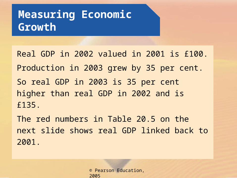
Real GDP in 2002 valued in 2001 is £100.
Production in 2003 grew by 35 per cent.
So real GDP in 2003 is 35 per cent higher than
real GDP in 2002 and is £135.
The red numbers in Table 20.5 on the next
slide shows real GDP linked back to 2001.
Measuring Economic Growth

© Pearson Education, 2005
Measuring Economic Growth
GDP in
Valued in prices inReal GDP
in 2001 prices2001 2002 2003
2001 £50 £50
2002 £100 £200 £100
2003 £270 £575 £135
© Pearson Education, 2005
Calculating the Price Level
The average level of prices is called the price level.
One measure of the price level is the GDP deflator, which is an average of current-year prices expressed as a percentage of the base-year prices.
Measuring Economic Growth
© Pearson Education, 2005
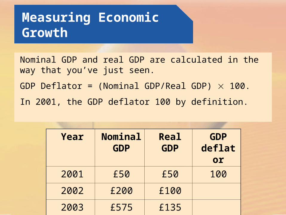
Nominal GDP and real GDP are calculated in the way that you’ve just seen.
GDP Deflator = (Nominal GDP/Real GDP) 100.
In 2001, the GDP deflator 100 by definition.
Year Nominal GDP
Real GDP
GDP deflator
2001 £50 £50 100
2002 £200 £100
2003 £575 £135
Measuring Economic Growth

© Pearson Education, 2005
In 2002, the GDP deflator is (£200/£100) 100 = 200.
In 2003, the GDP deflator is (£575/£135) 100 = 425.9.
Measuring Economic Growth
Year Nominal GDP
Real GDP
GDP deflator
2001 £50 £50 100
2002 £200 £100 200
2003 £575 £135 425.9

© Pearson Education, 2005
Deflating the GDP BalloonNominal GDP increases because production real GDP increases.
Measuring Economic Growth

© Pearson Education, 2005
Nominal GDP also increases because prices rise.
Measuring Economic Growth

© Pearson Education, 2005
We use the GDP deflator to let the air out of the nominal GDP balloon and reveal real GDP.
Measuring Economic Growth

© Pearson Education, 2005
Uses and Limitations of Real GDP
We use real GDP for three main purposes:
Economic welfare comparisons: Economic welfare is a comprehensive measure of the general state of well-being. International welfare comparisons: Real GDP is used to compare economic welfare in one country with that in another. Forecasts for stabilization policy: Real GDP is used to measure fluctuations in economic activity.

© Pearson Education, 2005
Catching the Wave
If you want a good economic ride, you must catch a wave.
But economic waves are hard to read.
What makes the economy ebb and flow in waves around its long-term growth trend?
Why do some wave rise high and then crash, and sometimes rise and roll on a long high?
How do waves in the global economy spread around the world?

© Pearson Education, 2005
Aggregate Supply
Aggregate Supply FundamentalsThe aggregate quantity of goods and services supplied depends on three factors:
1. The quantity of labour (L )2. The quantity of capital (K )3. The state of technology (T )
The aggregate production function shows how quantity of real GDP supplied, Y, depends on labour, capital and technology. The aggregate production function is written as the equation:
Y = F(L, K, T ).
© Pearson Education, 2005
Aggregate Supply
The labour market can be in any of three states:
1. Full employment
2. Above full employment
3. Below full employmentThe wage rate that makes the quantity of labour demanded equal to the quantity supplied is the equilibrium wage rate and the labour market is at full employment.
At full employment, real GDP is potential GDP and the unemployment rate is called the natural rate of unemployment.
© Pearson Education, 2005
Aggregate Supply
Long-run Aggregate Supply
The macroeconomic long run is a time frame that is sufficiently long for all adjustments to be made so that real GDP equals potential GDP and full employment prevails.
The long-run aggregate supply curve (LAS) is the relationship between the quantity of real GDP supplied and the price level when real GDP equals potential GDP.

© Pearson Education, 2005
This figure shows an LAS curve with potential GDP of £1,000 billion.
The LAS curve is vertical because potential GDP is independent of the price level.
Along the LAS curve all prices and wage rates vary by the same percentage so that relative prices and the real wage rate remain constant.
Aggregate Supply

© Pearson Education, 2005
Aggregate Supply
Short-run Aggregate SupplyThe macroeconomic short run is a period during which real GDP has fallen below or risen above potential GDP.
At the same time, the unemployment rate has risen above or fallen below the natural rate of unemployment.
The short-run aggregate supply curve (SAS) is the relationship between the quantity of real GDP supplied and the price level in the short run when the money wage rate, the prices of other factors of production and potential GDP remain constant.

© Pearson Education, 2005
Aggregate Supply
This figure shows a short-run aggregate supply curve.
Along the SAS curve, a rise in the price level with no change in the money wage rate and other factor prices increases the quantity of real GDP supplied the SAS curve is upward sloping.

© Pearson Education, 2005
Aggregate Supply
Movements along the LAS and SAS Curves
This figure summarizes what you’ve just learned about the LAS and SAS curves.

© Pearson Education, 2005
Aggregate Supply
Changes in Aggregate Supply
Aggregate supply changes if any influence on production plans other than the price level change.
Changes in Potential GDP (LAS) for three reasons: 1. Change in the full-employment quantity of labour; 2. Change in the quantity of capital; 3. Advance in technology.
Changes in SAS: Changes in the Money Wage rate and Other Resource Prices. A change in the money wage rate changes short-run aggregate supply and shifts the SAS curve. But a change in the money wage rate has no effect on long-run aggregate supply. The LAS curve does not shift.

© Pearson Education, 2005
Aggregate Supply
This figure shows how these factors shift the LAS curve and have the same effect on the SAS curve.
When potential GDP increases, both the LAS and SAS curves shift rightward.

© Pearson Education, 2005
Aggregate Supply
This figure shows the effect of a rise in the money wage rate on aggregate supply.
Short-run aggregate supply decreases and the SAS curve shifts leftward.
Long-run aggregate supply does not change and the LAS curve does not shift.

© Pearson Education, 2005
Aggregate Demand
The quantity of real GDP demanded, Y, is the total amount of final goods and services produced in the domestic economy that people, businesses, governments and foreigners plan to buy. This quantity is the sum of consumption expenditures, C, investment, I, government expenditures, G, and net exports, X – M. That is:
Y = C + I + G + X – M.
Buying plans depend on many factors and some of the main ones are: 1. The price level; 2. Expectations; 3. Fiscal policy and monetary policy; 4. The world economy
© Pearson Education, 2005
Aggregate Demand
The Aggregate Demand Curve
Aggregate demand is the relationship between the quantity of real GDP demanded and the price level.
The aggregate demand curve (AD) plots the quantity of real GDP demanded against the price level.
© Pearson Education, 2005
Aggregate Demand
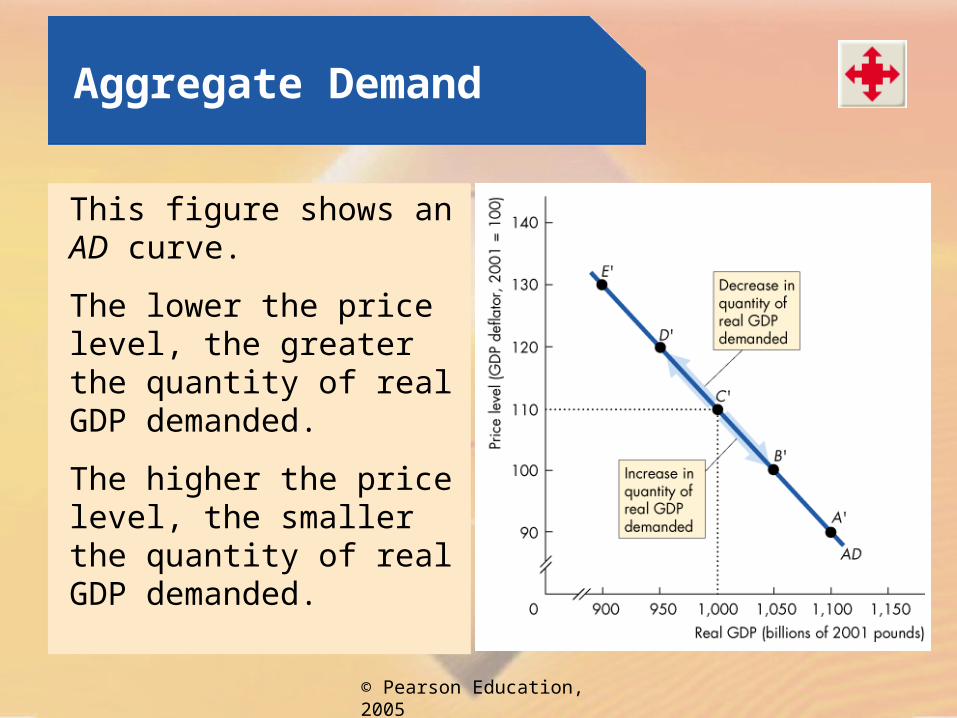
This figure shows an AD curve.
The lower the price level, the greater the quantity of real GDP demanded.
The higher the price level, the smaller the quantity of real GDP demanded.

© Pearson Education, 2005
Aggregate Demand
The AD curve slopes downward for two reasons:
Wealth effect
Substitution effects

© Pearson Education, 2005
Aggregate Demand
Changes in Aggregate Demand
A change in any influence on buying plans other than the price level changes aggregate demand.
The main influences on aggregate demand are:
Expectations Fiscal policy and monetary policy The world economy

© Pearson Education, 2005
Aggregate Demand
This figure illustrates changes in aggregate demand.
When aggregate demand increases, the AD curve shifts rightward…
… and when aggregate demand decreases, the AD curve shifts leftward.

© Pearson Education, 2005
Macroeconomic Equilibrium
Short-run Macroeconomic Equilibrium
Short-run macroeconomic equilibrium occurs when the quantity of real GDP demanded equals the quantity of real GDP supplied at the point of intersection of the AD curve and the SAS curve.

© Pearson Education, 2005
Macroeconomic Equilibrium
This figure illustrates a short-run macroeconomic equilibrium.
If real GDP is above equilibrium GDP, firms decrease production and lower prices…
… and if real GDP is below increase production and raise prices.

© Pearson Education, 2005
Macroeconomic Equilibrium
Long-run Macroeconomic Equilibrium
Long-run macroeconomic equilibrium occurs when real GDP equals potential GDP when the economy is on its LAS curve.
© Pearson Education, 2005
Macroeconomic Equilibrium
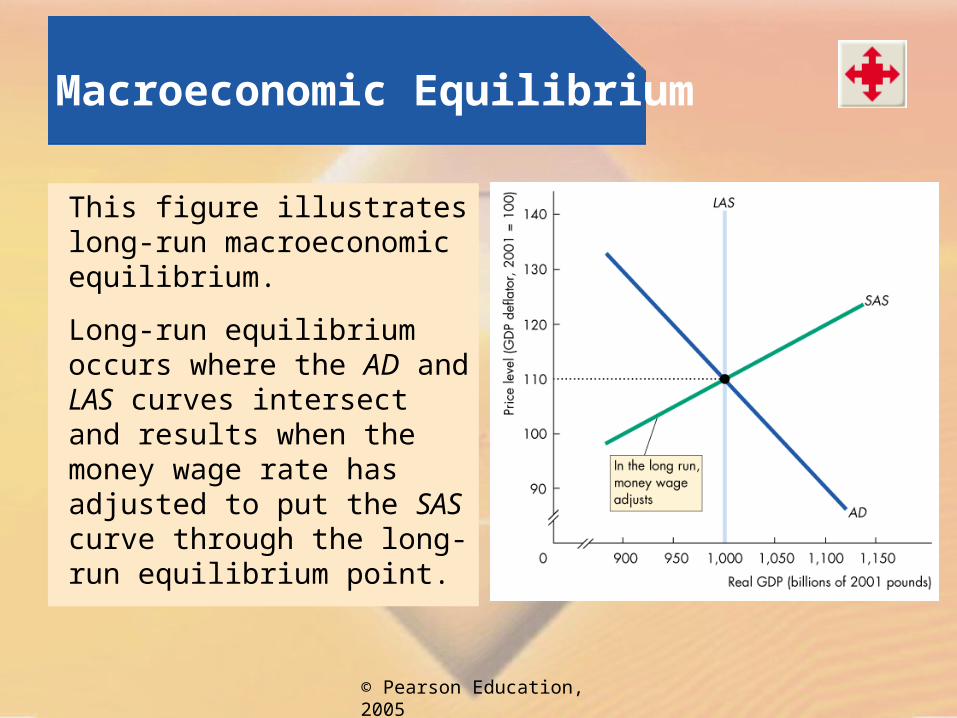
This figure illustrates long-run macroeconomic equilibrium.
Long-run equilibrium occurs where the AD and LAS curves intersect and results when the money wage rate has adjusted to put the SAS curve through the long-run equilibrium point.
© Pearson Education, 2005
Macroeconomic Equilibrium
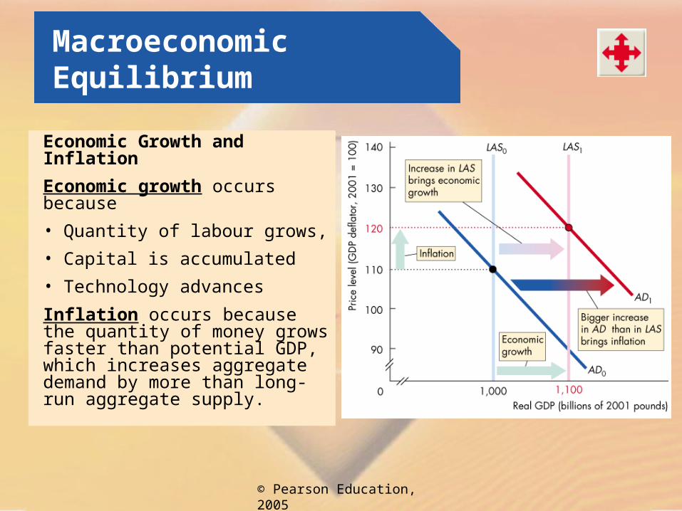
Economic Growth and Inflation
Economic growth occurs because
• Quantity of labour grows,
• Capital is accumulated
• Technology advances
Inflation occurs because the quantity of money grows faster than potential GDP, which increases aggregate demand by more than long-run aggregate supply.

© Pearson Education, 2005
Macroeconomic Equilibrium
The Business Cycle
The business cycle occurs because aggregate demand and the short-run aggregate supply fluctuate but the money wage rate does not change rapidly enough to keep real GDP at potential GDP.

© Pearson Education, 2005
Macroeconomic Equilibrium
A below full-employment equilibrium is an equilibrium in which potential GDP exceeds real GDP.
These figures illustrate below full-employment equilibrium.
The amount by which potential GDP exceeds real GDP is called a recessionary gap.

© Pearson Education, 2005
Macroeconomic Equilibrium
A long-run equilibrium is an equilibrium in which potential GDP equals real GDP.
These figures illustrate long-run equilibrium.

© Pearson Education, 2005
Macroeconomic Equilibrium
An above full-employment equilibrium is an equilibrium in which real GDP exceeds potential GDP.
These figures illustrate above full-employment equilibrium.
The amount by which real GDP exceeds potential GDP is called an inflationary gap.
© Pearson Education, 2005
Macroeconomic Equilibrium
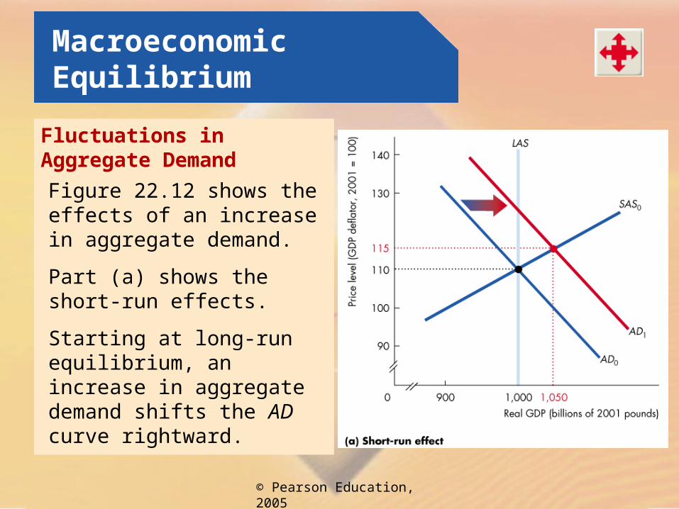
Fluctuations in Aggregate Demand
Figure 22.12 shows the effects of an increase in aggregate demand.
Part (a) shows the short-run effects.
Starting at long-run equilibrium, an increase in aggregate demand shifts the AD curve rightward.

© Pearson Education, 2005
Macroeconomic Equilibrium
Fluctuations in Aggregate DemandStarting at long-run equilibrium, an increase in aggregate demand shifts the AD curve rightward.
Firms increase production and raise prices a movement along the SAS curve.
In the short run, the economy is at above full-employment equilibrium.
© Pearson Education, 2005
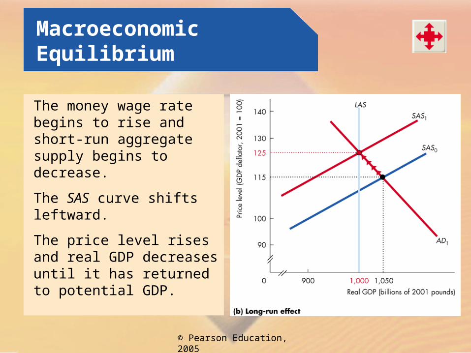
Macroeconomic Equilibrium
The money wage rate begins to rise and short-run aggregate supply begins to decrease.
The SAS curve shifts leftward.
The price level rises and real GDP decreases until it has returned to potential GDP.

© Pearson Education, 2005
Macroeconomic Equilibrium
Fluctuations in Aggregate SupplyThis figure shows the effects of a decrease in aggregate supply.
Starting at long-run equilibrium, a rise in the price of oil decreases short-run aggregate supply and the SAS curve shifts leftward.
Real GDP decreases and the price level rises.
The combination of recession and inflation is called stagflation.

© Pearson Education, 2005
Economic Growth, Inflation and Cycles in the UK Economy
From1963 to 2003:
Real GDP grew from £395 billion to £1,035 billion.
The price level rose from 8 to 106.
Business cycle expansions alternated with recessions.
© Pearson Education, 2005
Economic Growth, Inflation and Cycles in the UK Economy
Economic Growth
Real GDP growth was rapid during the 1960s and 1990s and slower during the 1970s and 1980s.
Inflation
Inflation was the most rapid during the 1970s.
Business Cycles
Recessions occurred during the mid-1970s, 1980–1982 and 1990–1992 (& 2008?)

© Pearson Education, 2005
Macroeconomic Schools of Thought
Macroeconomists divide into three broad schools of thought. We examine their views:
The Keynesian viewThe Classical viewThe Monetarist view