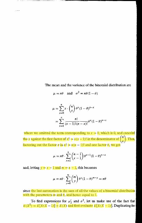
The mean and the variance of the binomial distribution are

J.L = nO and 0-2 = nO(l - 0)

n ,

L n. ------tf" (1 - O)n-x

- (x - l)!(n x)! x=l

where we omitted the term corresponding to x = 0, which is 0, and canceled

the x against the first factor of x! = x(x -1)! in the denominator of (:). Then,

factoring out the factor n in n! = n(n 1)! and one factor 0, we get

J.L = nO· t (: _ i) Ox-I (1 - ot-X

x=l

and, letting y = x - 1 and m = n -1, this becomes

since the last summation is the sum of all the values of a binomial distribution with the parameters m and 0, and hence equal to 1.

To find expressions for J.L~ and 0-2 , let us make use of the fact that

E(X2) = E[X(X 1)] + E(X) and first evaluate E[X(X -1)]. Duplicating for

and the book by H. G .. Itrejrere~nC(~s at the end of

four decimal places for use this table when e is

5.5. For instance, to Also, there ar~ several when n is large; one of

6.6. of the binomial

distribution are

is 0, and canceled

I'V"'-Ul~"V' of (;). Then,

e, we get

ne

a binomial distribution

use of the fact that - 1)]. Duplicating for

all practical purposes the steps used before, we thus get n

E[X(X -1)] = LX(x x=o

n ,

L n. x _----:---:--_----:ex (1 - e)n-= (x - 2)!(n x)! x=2

= n(n 1)e2 . t (; = D ex- 2(1 - e)n-x x=2

and, letting y = x 2 and m = n - 2, this becomes

Therefore,

and, finally,

E[X(X -1)] n(n -1)e2. t (~) eY(1- e)m-y

y=o

= n(n 1)e2

tL; = E[X (X - 1)] + E(X) n(n - 1)e2 + ne

(12 tL; tL2

= n(n 1)e2 + ne - n2e2

= ne(1- e) o An alternative proof of this theorem, requiring much less algebraic detail, is suggested in Exercise 5.6.

E(x) = ∑ x p(x) = ∑ x f(x) = ∑ x (1/N)

p(x=1) = π p(x=0) = 1 – π for n = 1 x f(x) x f(x) 0 1- π 0 1 π π

∑ 1 π = m’1 m’r = E(Xr) = π for r = 1, 2,3,4… m’1= E(X) = π m’2= E(X2) = π m2= E(X - π)2 = E(x2) – π2 = π - π2 = π (1 – π) = π q m3= π q (1 – 2π) m3 = E (x – π ) 3 = E(x3 - 3 x2 π + 3 x π 2 - π 3) = m’3 - 3 m’1 m’2 + 3 m’1

3 - m’13

= m’3 - 3 m’1 m’2 + 2 m’13

= π - 3 π 2 + 2 π 3

= π (1 – π) (1 – 2 π) = π q (1 – 2π) m4 = 3 (nπ q)2 + n π q (1-6 π q) (7.19)

)robability is given by

or numerically,

So i t would seem that your chances of getting an A by random trial are not very likely. How about settling for a C or better? If a C or better is to get a score of at least 7, we can calculate that probability too. But before you rush off to do that, wait a moment to think. Adding up all the probabilities from 7 to 20 is a pain; so instead why not add up the probabilities from 0 to 6 and subtract from l ? The an- swer is

S o by "guessing" you have a 94% chance of getting a C or better! You have only a 6% chance of failing the course. Now you know why professional testers, such as the Educational Testing Service in Princeton, deduct penalties for wrong answers-to pe- nalize guessing.

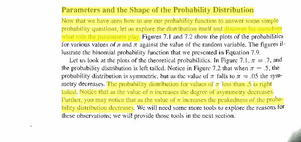
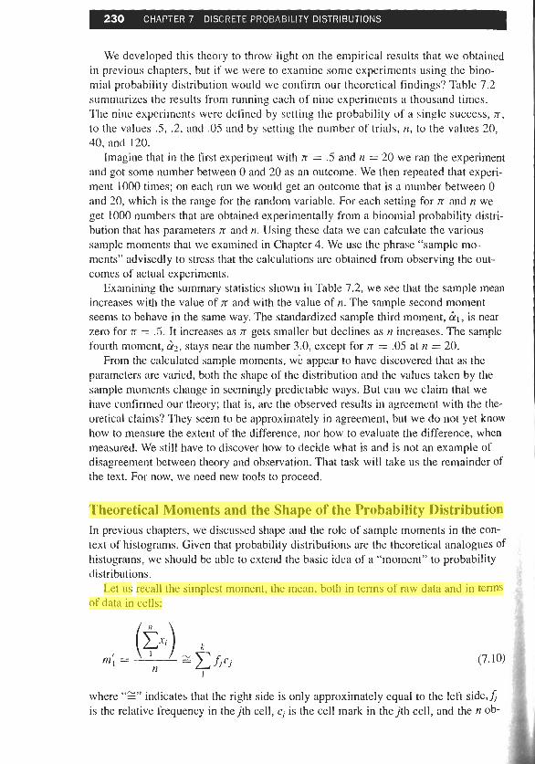
Now that we have seen how to use our probability function to answer some simple probability questions, let us explore the distribution itself and discover for ourselves what role the parameters play. Figures 7.1 and 7.2 show the plots of the probabilities for various values of n and rr against the value of the random variable. The figures il- lustrate the binomial probability function that we presented in Equation 7.9.

Let us look at the plots of the theoretical probabilities. In Figure 7.1, IT = .7, and the probability distribution is left tailed. Notice in Figure 7.2 that when rr = .5, the probability distribution is symmetric, but as the value of rr falls to n = .05 the sym- metry decreases. The probability distribution for values of rr less than .5 is right tailed. Notice that as the value of n increases the degree of asymmetry decreases. Further, you may notice that as the value of n increases the peakedness of the proba- bility distribution decreases. We will need some more tools to explore the reasons for these observations; we will provide those tools in the next section.

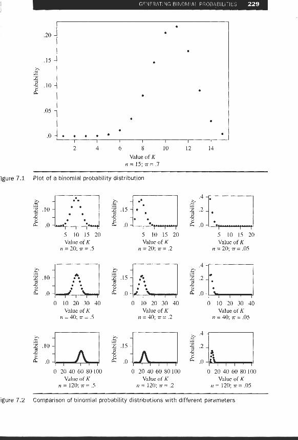
GENERATING BINOMIAL PROBABILITIES 229 1 - - - -

Value of K n = 15 ;n= .7

'igure 7.1 Plot of a binomial probability distribution

5 10 15 20 Value of K

n = 2 0 ; ~ = . 5

5 10 15 20 Value of K

n = 2 0 ; ~ = . 2

5 10 15 20 Value of K

n = 20; n = .05

0 10 20 30 40 0 10 20 30 40 0 10 20 30 40 Value of K Value of K Value of K

rr = 40: ~f = .5 n = 4 0 ; n = . 2 n = 40; n = .05

.0 I I I I I I

0 20 40 60 80 100 0 20 40 60 80 100 0 20 40 60 80 100 Value of K Value of K Value of K

n = 120; n = .5 11 = 120; ~f = .2 n = 120; T = .05

'igure 7.2 Comparison of binomial probability distributions with different parameters

We developed this theory to throw light on the empirical results that we obtained in prcvious chapters, but if we were to examine some experiments using the bino- i mial probability distribution would we confirm our theoretical findings? Table 7.2 summarizes the results from running each of nine experiments a thousand times. The nine experiments were defined by setting the probability of a single success, n, I

to the values .5, .2, and .05 and by setting the number of trials, 11, to the values 20, 40, and 120.

Imagine that in the first experiment with n = .5 and n = 20 we ran the experiment and got some number between 0 and 20 as an outcome. We then repeated that experi- ment 1000 times; on each run we would get an outcome that is a number between 0 and 20, which is the range for the random variable. For each setting for n and n we get 1000 numbers that are obtained experimentally from a binomial probability distri- bution that has parameters n and n. Using these data we can calculate the various sample moments that we exanlined in Chapter 4. We use the phrase "sample mo- ments" advisedly to stress that the calculations are obtained from observing the out- comes of actual experiments.

I

I

Examining the wmmary statistics shown in Table 7.2, we see that the sample mean 1

increases with the value of n and with the value of n. The sample second moment seems to behave In the same way. The standardized sarnpIe third moment, GI, is near zero for .ir = .5. It increases as n gets smaller but declines as rr increases. The sample fourth moment, G 2 , stays near the number 3.0, except for n = -05 at n = 20.

From the calculated sample moments, we appear to have discovered that as the parameters are varied, both the shape of the distribution and the values taken by the sample moments change in seemingly predictable ways. But can we claim that we have confirmed our theory; that is, are the observed results in agreement with the the- oretical claims? They seem to be approximately in agreement, but we do not yet know how to measure the extent of the difference, nor how to evaluate the difference, when measured. We still have to discover how to decide what is and is not an example of disagreement between theory and observation. That task will take us the remainder of the text. For now, we need new tools to proceed.

Theoretical Moments and the Shape of the Probability Distribution In previous chapters, we discussed shape and the role of sample moments in the con- text of histograms. Given that probability distributions are the theoretical analogues of histograms, we should be able to extend the basic idea of a "moment" to probability distributions.

Let us recall the simplest moment, the mean, both in terms of raw data and in terms of data in cells:

where ''2'' indicates that the right side is only approximately equaI to the left side,& is the relative frequency in the jth cell, c, is the cell mark in the jth cell, and the n ob-

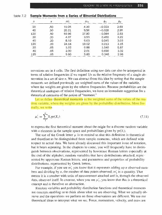
Table 7.2 Sample Moments from a Series of Binomial Dlstributions

n K m i m2 &I 2 2

20 .50 10.05 4.39 -0.023 2.69 40 .50 20.21 9.56 -0.028 2.95 120 .50 59.96 27.80 -0.084 2.93 20 .20 4.07 3.53 0.450 3.22 40 .20 8.10 6.63 0.045 3.03 120 .20 24.18 19.02 0.013 3.15 20 .05 1.02 0.88 1.040 5.87 40 .05 2.00 2.01 0.690 3.32 120 .05 5.93 5.80 0.340 2.96

servations are in k cells. The first definition using raw data can also be interpreted in terms of relative frequencies if we regard l ln as the relative frequency of a single ob- servation in a set of size n. We can abstract from this idea by noting that the sample moments we defined previously are weighted sums of the values of the variable, where the weights are given by the relative frequencies. Because probabilities are the theoretical analogues of relative frequencies, we have an immediate suggestion for a theoretical extension of the notion of "moment."

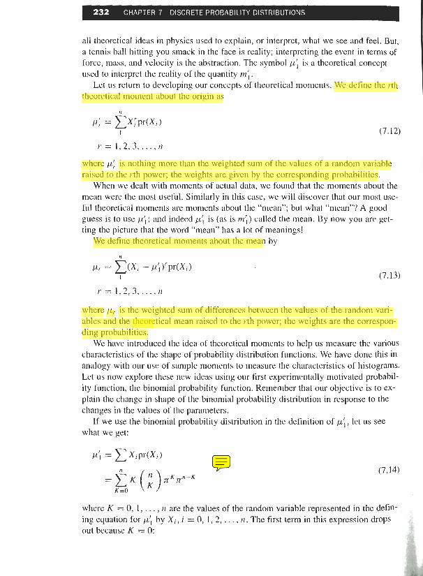
Let us define theoretical moments as the weighted sums of the values of the ran- dom variable, where the weights are given by the probability distribution. More for- mally, we write

to express the first theoretical moment about the origin for a discrete random variable with n elements in the sample space and probabilities given by pr(Xi).

The use of the Greek letter p is to remind us that this definition is theoretical and therefore to be distinguished from sample moments, which are defined with respect to actual data. We have already discussed this important issue of notation, but it bears repeating. In the chapters to come, you will frequently have to distin- guish between observations, represented by lowercase Roman letters especially at the end of the alphabet; random variables that have distributions attached, repre- sented by uppercase Roman letters, and parameters and properties of probability distributions, represented by Greek letters.

For example, if you see m', you know that it represents aclding up n observed num- bers and dividing by n, the number of data points observed; m', is a quantity. That means it is a number with units of measurement attached and is, through the observed data, observed itself. In contrast, when you see /A', , you know that this is a theoretical concept and is therefore an abstraction.

Random variables and probability distribution functions and theoretical moments are concepts enabling us to think about what we are observing. What we actually ob- serve and the operations we perform on those observations are different. We use our theoretical ideas to interpret what we see. Force, momentum, velocity, and mass are

all theoretical ideas in physics used to explain, or interpret, what we see and feel. But, a tennis ball hitting you smack in the face is reality; interpreting the event in tenns of force, Inass, and velocity is the abstraction. The symbol ~ c ' , is a theoretical concept used to interpret the reality of the quantity m', .

Let us return to developing our concepts of theoretical moments. We define the rth theoretical moment about the origin as

where is nothing more than the weighted sum of the values of a random variable raised to the rth power; the weights are given by the corresponding probabilities.

When we dealt with moments of actual data, we found that the moments about the mean were the most useful. Similarly in this case, we will discover that our most use- ful theoretical moments are monients about the "niean"; but what "niean"? A good guess is to use p',; and indeed CL', is (as is M',) called the mean. By now you are get- ting the picture that the word "mean" has a lot of meanings!

We define theoretical monients about the ineaii by

where /A,- is the weighted sum of differences between the values of the random van- ables and the theoretical mean raised to the r-th power; the weights are the correspon- ding probabilities.

We have introduced the idea of theoretical moments to help us measure the various characteristics of the shape of probability distribution functions. We have done this in analogy with our use of sample moments to measure the characteristics of histograms. Let us now explore these new ideas using our first experimentally motivated probabil- ity function, the binomial probability function. Remember that our objective is to ex- plain the change in shape of the binomial probability distribution in response to the changes in the values of the parameters.

If we use the binomial probability distribution in the definition of pi , let us see what we get:

where K = 0, 1, . . . , I ? are the values of the random variable represented in the defin- ing equation for pi by Xi, i = 0, I, 2, . . . , n. The first term in this expression drops <r

out because K = 0:

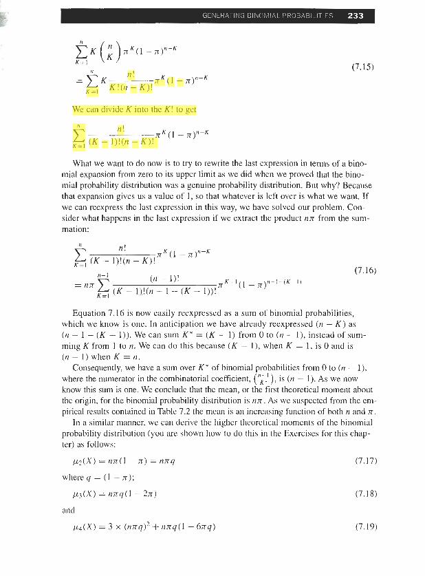
What we want to do now is to try to rewrite the last expression in terms of a bino- mial expansion from zero to jts upper limit as we did when we proved that the bino- mial probability distribution was a genuine probability distribution. But why? Because that expansion gives us a value of 1, so that whatever is left over is what we want. If we can reexpress the last expression in this way, we have solved our problem. Con- sider what happens in the last expression if we extract the product nrr from the sum- mation:

n! 2 (K - l)!(n - K)! ir (1 - 7ry-K

K=l

Equation 7.16 is now easily reexpressed as a sum of binomial probabilities, which we know is one. In anticipation we have already reexpressed (n - K ) as ( n - 1 - (K - I)). We can sum K* = (K - 1) from 0 to (n - I ) , instead of sum- ming K from I to tz. We can do this because (K - I), when K = 1, is 0 and is (n - I ) when K = t z .

Consequently, we have a sum over K* of binomial probabilities from 0 to (I! - I ) , where the numerator in the combinatorial coefficient, (IF,;'), is (n - 1). As we now know this sum is one. We conclude that the mean, or the first theoretical moment about the origin, for the binomial probability distribution is nir. As we suspected from the eni- pirical results contained in Table 7.2 the mean is an increasing function of both n and i r .

In a similar manner. we can derive the higher theoretical niomenls of the binomial probability distribution (you are shown how to do this in the Exercises for this chap- ter) as follows:

where q = (1 - ir);

and

Before we start to use these theoretical moments to represent the shape of the prob- ability distribution, we recognize from our experience in Chapter 6 that it is probably important to standardize the theoretical moments beyond the second to allow for both origin and scale effects, just as we had to do for the higher sample moments.

Following the precedent set in previous chapters, we define

where a, and a2 are the standardized theoretical moments in the sense that any change in the origin for measuring the random variable or in the chosen scale for measuring the random variable will leave the value of the standardized third and fourth theoretical moments invariant. For example, if the random variable represents temperature readings, then the values of a1 and a2 are the same no matter whether the temperature readings are recorded in degrees Fahrenheit or degrees Celsius.

Notice that the "little hats" are gone from al and a2. This is because we are now dealing with the theoretical entities and not their sample analogues. If we were to use our usual practice, we would have written a1 and a2 for the sample standardized mo- ments in agreement with using m, for p,, but as you now see that would have been an unfortunate choice given our use of a for so many other terms. This trick of using lit- tle hats to indicate that we are talking about the sample analogues, not the theoretical quantities, will be used quite extensively in the next few chapters.

Let us write down our first two theoretical moments, followed by our standardized third and fourth theoretical moments for the binomial probability distribution:

p', = n x ; ~2 = nrrq

where q = (1 - rr);

We can now explore the relationship between theoretical moments, parameters, and the shape of the probability function. Let us review the summary calculations

I GENERATING BINOMIAL PROBABILITIES 235 1

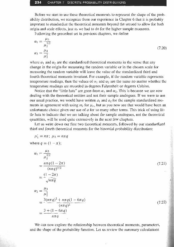
Table 7.3 Theoretical Moments for the Binomial Distrlbutlon for Various Parameters 51 Parameter Values Theoretical Moments

n n L L ~ PZ 012

20 .50 10 5.00 0.00 3.15 20 .20 4 3.20 0.33 3.26 20 .05 1 0.95 0.92 4.00 40 .50 20 10.00 0.00 3.08 40 .20 8 6.40 0.24 3.13 40 .05 2 1.90 0.65 3.50 120 .50 60 30.00 0.00 3.03 120 .20 24 19.20 0.13 3.04 120 .05 6 5.70 0.35 3.17

shown in Table 7.3 and the plots of the theoretical probabilities shown in Figure 7.2 to see the extent to which our theoretical results are useful. For the nine alternative combinations of n and n that we have examined, we should conipare the theoretical moments with the values obtained for the sample moments using the experimental data summarized in Table 7.2.

On comparing the theoretical values with the values obtained from the experi- ments, we observe a close, but by no means exact relationship, between the two sets of numbers. Thinking about these numbers and their comparisons, we may realize that a major problem that faces us is how to decide what is and is not close. How do we decide when an empirical result "confirms" the theoretical statement, given that we know that it is most unlikely that we will ever get perfect agreement between the- ory and observation? This is an important task that will have to be delayed until Chapter 9.

The values for the theoretical moments listed in Table 7.3 and the expressions that we derived for the theoretical moments enable us to confirm the conjectures that we formulated on first viewing the summary statistics in Table 7.2. We see even more clearly from the algebraic expressions that pi increases in 11 and n; that p 2 increases in rz and n up to .5; that the standardized third and fourth theoretical moments de- crease in n to minimum values that are 0.00 and 3.03, respectively. As n approaches 0 or I both cr l and a 2 get bigger for any given value of 11; alternatively expressed, the minimum for both I crl l and crz is for n = .5.

The effect that n has 011 the shape of the distribution is quite remarkable. No matter ho\v asynunetric the distribution is to begin with, a sufiiciently large increase in n will produce a distribution that is very synunetric; the symmetry is measured by the value of c r ~ . The limit as n -+ oo for crl is 0, and the limit for cr2 is 3. We will soon see that these two values for crl and keep occurring as the limits for the values of crl and cr2 as a pa- rameter n gets bigger and bigger. We might suspect that these particular values for the theoretical moments represent a special probability distribution, as indeed they do.

Consider a simple example. Suppose that the distribution of births by sex within a specified region over a short interval of time is given by the binomial distribution with parameters 11, being the total number of births in the region, and n, the probability of a male birth. Usually, the value of n is n little greater than .5, say .52. If 11 = 100, the

mean of the distribution, p', = nx = 52. What this means is that the value about which actual numbers of male births v i~ies is 52; for any given ti~ne period it might be less, or it might be more, but over n long period we expect the variations to average approxi- niately 52.

The square root of the variance of the distribution is given by Jnn( l - IT), which in this case is 5. We can expect very approximately that about 90% of the t i~ne the nunlber of male births will lie between 42 and 62. Certainly, we would be very sur- prised if the number of male births fell below 37 or exceeded 67.

Given that the standardized third liioment is negative, but very smail, this distribution is approxin~ately symmetric about 52; it is equi~lly likely to have fewer than 52 male births as it is to have more. The standardized fourth moment is not too much less than 3, so that we call conclude that our distribution has neither thin tails nor Cat ones. Very large and very s~nall numbers of male births are neither very frequent nor very rare.

We can summarize this section by pointing out that what we have discovered is that

the conditions of an experiment determine the shape of the relevant probability function. the effect.\ of the experimental conditions are reflected in the values taken by the parameters of the distribution. the shape of the distribution is measured in terms of the theoretical moments of the probability function. the theoretical moments are then~selves functions of the parameters.

Expectation This section is not what you might expect; it is about a very useful operation in statis- tics called taking the expected value of a random variable, or expectation. You have in fact already done it-that is, taken an expectation of a random variable-but you did not kno\v it at the time. The operation that we used to determine the theoretical moments was an example of the procedure known as expectation. Once again, we will be able to obtain both insight into and ease of manipulation of random variables and their properties by generalizing a specific concept and thereby extending our theory.

Taking expected values is nothing more than getting the weighted sums of func- tions of random variables, where the weights are provided by the probability function. Let us define the concepl of expectation formally as follows:

The expected value of any function of a random variable, X, say g(X) , is given by

We have already pel-formed this operation several times while calculating the theoretical moments. For p',, the function g(X) was just X; for p~ the function g ( X ) was (X - and so on. The function g(X) can be any function you like. What- ever choice you make, the expectation of g(X), however defined, is given by Equa- tion 7.23.

Consider the simple coin toss experiment with probability function discussed in Chapter 6. The distribution function was

The expectation of X,

takes the value in the case of a true coin toss. Note that I used the notation Ex to indicate "summation over the values of X."

What does this simple result mean? Clearly, it does not mean that in a coin toss one observes "i" on average. All one obsei-ves is a string of 0s and Is, not a single in sight. What the "average," or "mean," of the variable given by the expectation opera- tion implies is that it is the value for which the average deviation is zero. Recall from Chapter 3 that we define the sample mean as that value such that the average devia- tions from it are zero; that is

Similarly, we note that EL', satisfies

where

Recalling our definition of a random variable (which is a function on all subsets of a sample space to the real numbers), we recognize that ,p(X) is also a random variable. This is because it is a function of a random variable that is, in turn, a function of subsets of some sample space, so that g(X), through X, is itsclf a ran- dom variable. As such g(X) will have associated with it a corresponding probabil- ity function, say h(Y), where Y = g(X). For the student comfortable in calculus this approach is explored in the Exercises in terms of the concept lermed "transfor- mation of variables."

But we have also seen that ally probability function has associatetl with it a set of theoretical moments. The first of these is the mean, or p', . From the defini~ion of p', ,

p; = C Y;h(Y;) (7.24)

where Y; = g(X;) and h(Y;) is the probability function for the random variable Yi. Let's make sure that we understand what is going on here. We began with a

random variable Xi, i = 1,2 , . . . , n, with corresponding probability function f(Xi). We then decided to create a new random variable Y, with values Y,, by defining Y; = g(X;), for example, Y; = ( X i - We have claimed that there is some probability function, say h(Y;), that provides the distribution of probabilities for the random variable Y. At the moment we do not know how to find the probability

238 CHAPTER 7 DISCRETE PROBABILITY DISTRIBUTIONS

function h(Yi), but because we know that Y is a random variable, we do know that there exists sonie probability function for the random variable Y: wc are just giving i t a name.

So if we knew the probability function lt(Yi), we could obtain the mean of the random variable Y. But that is often a problem; i t is sometimes not casy to get the probability function h(Y,) frorn inform~ition on X,, g(Xi), and f(X,). Hcre is where the operation of expectation comes to the rescue. Using the expression for expectation, we I~ave

where pr(X,) is thc probability function for the random variable X. From this expres- sion, we see that we can get the mean of the random variable Y = g(X) without ha\!- ing to find out what the probability fiinction Ir(Y) is. We have in fact the result

All the theoretical niomellts are examples of expeclations; w', is the expectation of the random variable X; b 2 ( X ) is the expectation of the randorn variable (X - w ' , ) ~ ; and so on. As we know, all of these theoretical moments are merely weighted sums of the values of the appropriate function of the randorn variable X. The weight5 are given by the probabilities associated with cach value of X or u.ith each value of some func- tion of X.

You might get a better feel for the idea of expectation if we consitler a case where the number of variable valuea is two:

and n is the probability that X = XI and (I - n) is the probability that X = X2. Suppose that X I = 1 , X2 = 2, and that we let n have various values. As an exam-

ple. you might be contemplating an investment opportunity in which there are two possible outcornes: $1,000 in one case and $2,000 in the other; the probability of the first case occurring is represented by n .

Let us try n = I , :, i, $, and 0. For each of these values of n, recall that (I - n) will have values 0, $, i , a , and 1 . We can write down for each choice of n the corre- sponding value of the expectation

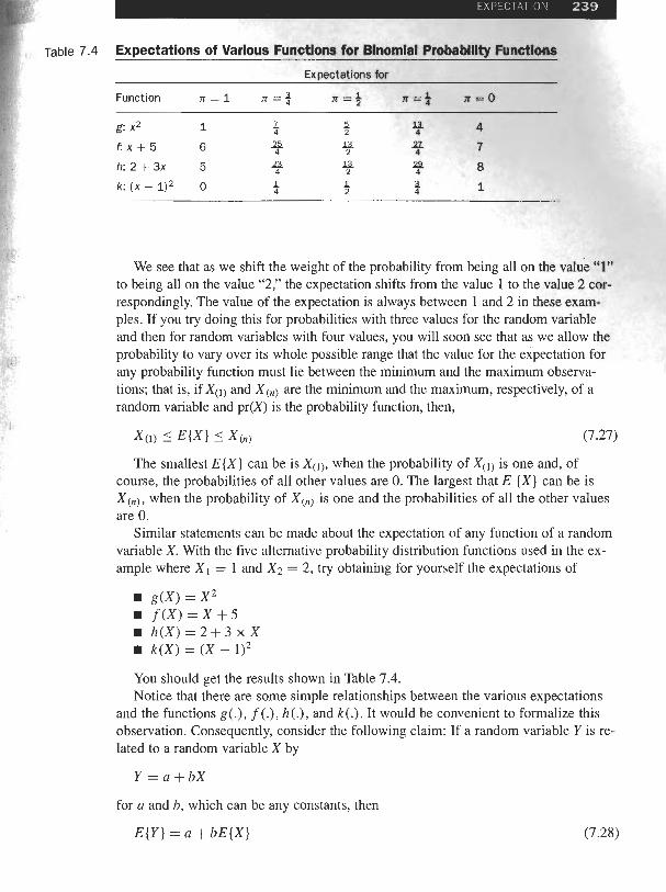
Table 7.4 Expectations of Various Functlons for Binomial Probability Functions

Expectations for

Function n = l n = + n = l - 2 ~~1 x = O

g: x2 1 - 7 4 3 +? 4 f x f 5 6 f 9 $ 7

h: 2 + 3x 5 ?- 9 9 8

k: ( x - 1)' 0 $ 3 2 1

We see that as we shift the weight of the probability from being all on the va~uk L41'' to being all on the value "2," the expectation shifts from the value 1 to the value 2 cor- respondingly. The value of the expectation is always between 1 and 2 in these exam- ples. If you try doing this for probabilities with three values for the random variable and then for random variables with four values, you will soon see that as we allow the probability to vary over its whole possible range that the value for the expectation for any probability function must lie between the minimum and the maximum observa- tions; that is, if X ( , ) and X $ ) are the minimum and the maximum, respectively, of a random variable and pr(X) is the probability function, then,

The smallest E ( X ) can be is XO) , when the probability of X( , , is one and, of course, the probabilities of all other values are 0. The largest that E ( X ) can be is X g ) , when the probability of X(, ,) is one and the probabilities of all the other values are 0.

Similar statements can be made about the expectation of any function of a random variable X . With the five alternative probability distribution functions used hl the ex- ample where X I = 1 and X 2 = 2 , try obtaining for yourself the expectations of

You should get the results shown in Table 7.4. Notice that there are some simple relationships between the various expectations

and the functions g(.), f (.), A ( . ) , and k ( . ) . It would be convenient to formalize this observation. Consequently, consider the following claim: If a random variable Y is re- lated to a random variable X by

for a and b, which can be any constants, then

You can easily demonstrate this for yourself by substituting the definition of Y into the definition for expectation:

What if we define Y by

where the (XI) are a Fet of 11 random variables. Suppose that the expectations of the X,, i = 1,2. . . . , ri are C I , ~ 2 , . . . , e,, respectively; that is, E{X,) = 6,. What is the ex- pectation of Y in terms of the E(Xl]?

By a slight extension of the preceding argument we see that

where pr(Xl)pr(X2) . . . pr(X,,) is the joint probability function for the ri randonl vari- ables (XI ) , i = 1,2 , . . . , n , assuming that the (XI) are statistically independent.

Applying the elementary probability concepts that we learned in Chapter 6, we see that

where Xjj represents the jth value of the ith random variable. So

In the chapters to come we will use these concepts and results repeatedly, so make sure that you thoroughly understand these ideas.

Let us try a simple example using the random variables XI and X2, where E ( X l ) = 3, E(x:] = 9, and E(X2) = 4. Let us assume that we know nothing fur- ther about the distributions of XI and X2. TO find the expectation of

and of

we obtain by sllbstitution

E ( Y ) = 2 x 3 + 5 x 4

= 26

E(CV) = E(x:] + 4 - E ( 4 X l )

= 9 + 4 - ( 4 x 3 ) = 1

In Equation 7.30, we defined the expectation of a "sum of variables" with respect to random variables that were independently distributed. Let us now extend that defi- nition to variables that are not independently distributed. Let F(XI, X2) be the joint distribution of XI, X? where F(XI, X2) cannot be factored into the product of the mar- ginal~. Consider:

111 this development, we used the result that the marginal distribution is obtained from the joint distribution by adding up the probabilities over the "other variable" (as was discussed in Chapter 6); Cx2F (XI , X2) = FI (X I ) . The notation implies that one sums over the values of both XI and X2. In the previous expression, we used the idea that

where FI(XI) is the marginal distribution of XI. We can easily extend this idea to weighted sums of funclions of the variables, one

at a time. For example,

So far, it would seem that there is no difference between the independent and the nonindependent cases. Thai is because we have not looked at any functions invol\~ing the protlucts of XI and X2. Consider, using the same distribution:

No further simplification is possible. However, if the variables XI and X2 are inde- pendent, the situation is different:

Let us explore this result using the simple bivariate distribution defined in Chapter 6. Table 6.4 gave the joint distribution of XI = (0, 1) and X2 = (- 1,0 , I ) . We obtain

where all other terms have dropped out because zeros are involved in the multiplica- tion. In contrast, consider the expectation of the product of the independent random variables (Yl, Y2] that were defined in Table 6.6 and have the same marginal distribu- tions as those of (XI, X2}.

after having dropped all terms involving multiplication by zero. So even for two dis- tributions where the values taken by the random variables are the same and the mar- ginal probabilities are the same, there is a considerable difference in the expectation of a product between variables that are independent and nonindependent.